A Pyrrhic Victory?

Bank Bailouts and Sovereign Credit Risk∗

Viral V. Acharya

NYU-Stern, CEPR and NBER

Itamar Drechsler

NYU-Stern

Philipp Schnabl

NYU-Stern and CEPR

January 2012

Abstract

We show that financial sector bailouts and sovereign credit risk are intimately linked.

A bailout benefits the economy by ameliorating the under-investment problem of the

financial sector. However, increasing taxation of the non-financial sector to fund the

bailout may be inefficient since it weakens its incentive to invest, decreasing growth.

Instead, the sovereign may choose to fund the bailout by diluting existing government

bondholders, resulting in a deterioration of the sovereign’s creditworthiness. This dete-

rioration feeds back to the financial sector, reducing the value of its guarantees and ex-

isting bond holdings as well as increasing its sensitivity to future sovereign shocks. We

provide empirical evidence for this two-way feedback between financial and sovereign

credit risk using data on the credit default swaps (CDS) of the Eurozone countries and

their banks for 2007-11. We show that the announcement of financial sector bailouts

was associated with an immediate, unprecedented widening of sovereign CDS spreads

and narrowing of bank CDS spreads; however, post-bailouts there emerged a signifi-

cant co-movement between bank CDS and sovereign CDS, even after controlling for

banks’ equity performance, the latter being consistent with an effect of the quality of

sovereign guarantees on bank credit risk.

∗We are grateful to Stijn Claessens, Ilan Kremer, Mitchell Petersen, Isabel Schnabel and Luigi Zingales(discussants), Dave Backus, Mike Chernov, Paul Rosenbaum, Amir Yaron, Stan Zin, and seminar participantsat the 2011 AEA Meetings, 2011 EFA Meetings, 2011 NBER Summer Institute, Austrian Central Bank,Bundesbank-ECB-CFS Joint Luncheon workshop, Douglas Gale’s Financial Economics workshop at NYU,Federal Reserve Bank of Minneapolis, HEC Paris and BNP Paribas Hedge Fund Center conference, IndianSchool of Business, Indian Institute of Management (Ahmedabad), London Business School and Moody’sCredit Risk Conference, Oxford Said Business School, Rothschild Caesarea Center 8th Annual Conference(Israel), Stockholm School of Economics and SIFR, Universitat van Amsterdam and de Nederlandsche Bank,and University of Minnesota for helpful comments. Farhang Farazmand and Nirupama Kulkarni providedvaluable research assistance. Please send all correspondence to Viral Acharya (vacharya@stern.nyu.edu),Itamar Drechsler (itamar.drechsler@stern.nyu.edu), and Philipp Schnabl (pschnabl@stern.nyu.edu).

1 Introduction

Just three ago, there was essentially no sign of sovereign credit risk in the developed economies

and a prevailing view was that this was unlikely to be a concern for them in the near future.

Recently, however, sovereign credit risk has become a significant problem for a number of de-

veloped countries, most notably in Europe. In this paper, we are motivated by three closely

related questions surrounding this development. First, were the financial sector bailouts an

integral factor in igniting the rise of sovereign credit risk in the developed economies? We

show that they were. Second, what was the exact mechanism that caused the transmission

of risks between the financial sector and the sovereign? To understand this, we propose a

model wherein the government can finance a bailout through both increased taxation and

via dilution of existing government debt-holders. The bailout is beneficial; it alleviates a

distortion in the provision of financial services. However, both financing channels are costly.

Increased taxation reduces the non-financial sector’s incentives to invest. Therefore, when

the optimal bailout is large, dilution can become a relatively attractive option, leading to de-

terioration in the sovereign’s creditworthiness. Finally, we ask whether there is also feedback

going in the other direction– does sovereign credit risk feed back to the financial sector? We

explain – and verify empirically – that such a feedback is indeed present, due to the financial

sector’s implicit and explicit guarantees and holdings of sovereign bonds.

Our results call into question the usually implicit assumption that government resources

are vastly deep and that the main problem posed by bailouts is that of moral hazard –

that is, the distortion of future financial sector incentives. While the moral hazard cost is

certainly pertinent, our conclusion is that bailout costs are not just in the future. They are

tangible right around the timing of bailouts and are priced into the sovereign’s credit risk

and cost of borrowing. Thus, aggressive bailout packages that stabilize financial sectors in

the short run but ignore the ultimate taxpayer cost might end up being a Pyrrhic victory.

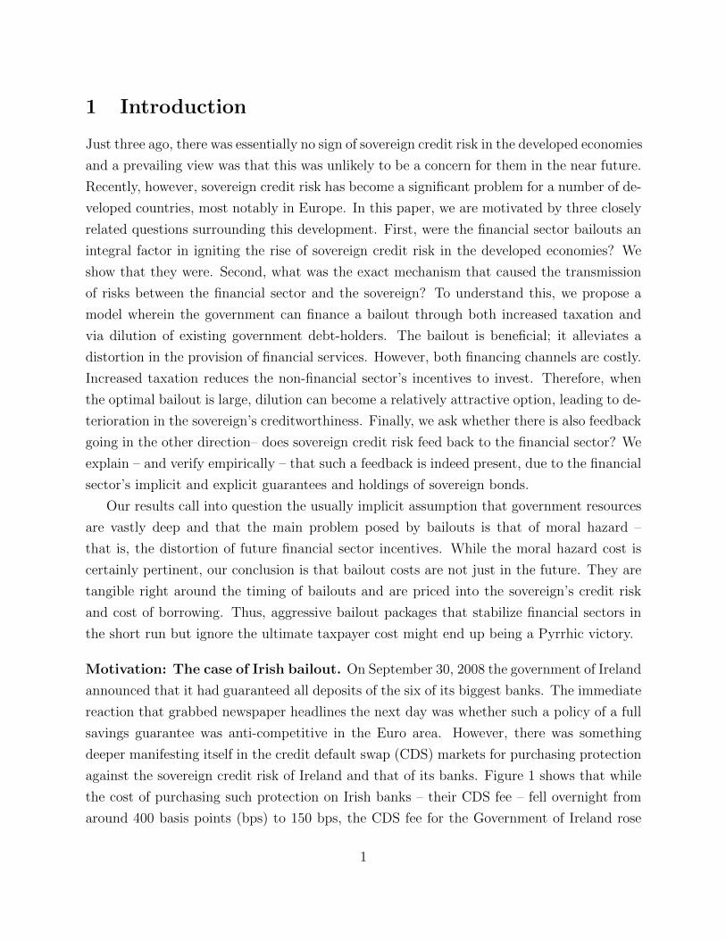
Motivation: The case of Irish bailout. On September 30, 2008 the government of Ireland

announced that it had guaranteed all deposits of the six of its biggest banks. The immediate

reaction that grabbed newspaper headlines the next day was whether such a policy of a full

savings guarantee was anti-competitive in the Euro area. However, there was something

deeper manifesting itself in the credit default swap (CDS) markets for purchasing protection

against the sovereign credit risk of Ireland and that of its banks. Figure 1 shows that while

the cost of purchasing such protection on Irish banks – their CDS fee – fell overnight from

around 400 basis points (bps) to 150 bps, the CDS fee for the Government of Ireland rose

1

sharply. Over the next month, this rate more than quadrupled to over 100 bps and within

six months reached 400 bps, the starting level of its financial firms’ CDS. While there was

a general deterioration of global economic health over this period, the event-study response

in Figure 1 suggests that the risk of the financial sector was substantially transferred to the

government balance sheet, a cost that Irish taxpayers must eventually bear.

Viewed in the Fall of 2010, this cost rose to dizzying heights prompting economists to

wonder if the precise manner in which bank bailouts were awarded had rendered the financial

sector rescue exorbitantly expensive. Just one of the Irish banks, Anglo Irish, has cost the

government up to Euro 25 billion (USD 32 billion), amounting to 11.26% of Ireland’s Gross

Domestic Product (GDP). Ireland’s finance minister Brian Lenihan justified the propping up

of the bank “to ensure that the resolution of debts does not damage Ireland’s international

credit-worthiness and end up costing us even more than we must now pay.” Nevertheless,

rating agencies and credit markets revised Ireland’s ability to pay future debts significantly

downward. The original bailout cost estimate of Euro 90 billion was re-estimated to be 50%

higher and the Irish 10-year bond spread over German bund widened significantly, ultimately

leading to a bailout of Irish government by the stronger Eurozone countries.1

This episode is not isolated to Ireland though it is perhaps the most striking case. In

fact, a number of Western economies that bailed out their banking sectors in the Fall of

2008 have experienced, in varying magnitudes, similar risk transfer between their financial

sector and government balance-sheets. Our paper develops a theoretical model and provides

empirical evidence that help understand this interesting phenomenon.

Model. Our theoretical model consists of two sectors of the economy – “financial” and

“corporate” (more broadly this includes also the household and other non-financial parts of

the economy), and a government. The two sectors contribute jointly to produce aggregate

output: the corporate sector makes productive investments and the financial sector invests in

intermediation “effort” (e.g., information gathering and capital allocation) that enhance the

return on corporate investments. Both sectors, however, face a potential under-investment

problem. The financial sector is leveraged (in a crisis, it may in fact be insolvent) and

under-invests in its contributions due to the well-known debt overhang problem (Myers,

1977). We assume that restructuring this financial sector debt is impossible or prohibitively

expensive. For simplicity, the corporate sector is un-levered. However, if the government

1See “Ireland’s banking mess: Money pit – Austerity is not enough to avoid scrutiny by the markets”,the Economist, Aug 19th 2010; “S&P downgrades Ireland” by Colin Barr, CNNMoney.com, Aug 24th 2010;and, “Ireland stung by S&P downgrade”, Reuters, Aug 25th, 2010.

2

undertakes a “bailout” of the financial sector, in other words, makes a transfer from the

rest of the economy that results in a net reduction of the financial sector debt, then the

transfer must be funded in the future (at least in part) through taxation of corporate profits.

Such taxation, assumed to be proportional to corporate sector output, induces the corporate

sector to under-invest.

A government that is fully aligned with maximizing the economy’s current and future

output determines the optimal size of the bailout. We show that tax proceeds that can be

used to fund the bailout have, in general, a Laffer curve property (as the tax rate is varied),

so that the optimal bailout size and tax rate are interior. In practice, governments fund

bailouts in the short run by borrowing or issuing bonds, which are repaid by future taxation.

There are two interesting constraints on the bailout size that emerge from this observation.

One, the greater is the existing debt of the government, the lower is its ability to undertake

a bailout. This is because the Laffer curve of tax proceeds leaves less room for the government

to increase tax rates for repaying its bailout-related debt. Second, the announcement of the

bailout lowers the price of government debt due to the anticipated dilution from newly issued

debt. Interestingly, if the financial sector of the economy has assets in place that are in the

form of government bonds (which is typically the case), then the bailout is in fact associated

with some “collateral damage” for the financial sector itself.2 Illustrating the possibility of

such a two-way feedback is a novel contribution of our model.

If the financial sector crisis is severe and existing government debt is large, then the

under-investment cost of fully funding with tax revenue both existing government debt and

a bailout are high, and the government may undertake a strategic default. Assuming that

there are some deadweight costs of such default, for example, due to international sanctions or

from being unable to borrow in debt markets for some time, we derive the optimal boundary

for sovereign default as a function of its pre-bailout debt and the financial sector’s liabilities.

This boundary explains that a heavily-indebted sovereign faced with a heavily-insolvent

financial sector will be forced to “sacrifice its credit rating” to save the financial sector and

at the same time sustain economic growth.

We then extend the model to allow for uncertainty about the realized output growth of

the corporate sector. This introduces a possibility of solvency-based default on government

debt. Interestingly, given the collateral damage channel, an increase in uncertainty about

2For example, in mid 2011 the exposure of UniCredit and Intesa (two big Italian banks) to Italian bondswas 121 percent and 175 of their core capital. In Spain, the ratios for the two biggest banks, BBVA andSantander, were 193 percent and 76 percent, respectively. See “Europe’s Banks Struggle With Weak Bonds”by Landon Thomas Jr., NYTimes.com, August 3, 2011.

3

the sovereign’s economic output not only lowers its own debt values but also increases the

financial sector’s risk of default. This is because the financial sector’s government bond

holdings fall in value, and (in an extension of the model) so do the value of the government

guarantees accorded to the financial sector as a form of bailout. In turn, these channels

induce a post-bailout co-movement between the financial sector’s credit risk and that of the

sovereign, even though the immediate effect of the bailout is to lower the financial sector’s

credit risk and raise that of the sovereign.

Empirics. Our empirical work analyzes this two-way feedback between the financial sector

and sovereign credit risk. Our analysis focuses mainly on the Western European economies

during the financial crisis of 2007-11.

We examine sovereign and bank CDS in the period from 2007 to 2011 and find three

distinct periods. The first period covers the start of the financial crisis in January 2007

until the first bank bailout announcement. This period includes the bankruptcy of Lehman

Brothers. Across all Western economies, we see a large, sustained rise in bank CDS as the

financial crisis develops. However, sovereign CDS spreads remain very low. This evidence

is consistent with a significant increase in the default risk of the banking sector with little

effect on sovereigns in the pre-bailout period.

The second period covers the bank bailouts starting with the announcement of a bailout

in Ireland in late September 2008 and ending with a bailout in Sweden in late October 2008.

During this one-month period, we find a significant decline in bank CDS across all countries

and a corresponding increase in sovereign CDS. This evidence suggests that bank bailouts

produced a transfer of default risk from the banking sector to the sovereign.

The third period covers the period after the bank bailouts and until 2011. We find that

both sovereign and bank CDS increased during this period. Consistent with our model’s

predictions, the increase was larger for countries whose public debt ratios were higher and

whose financial sectors were more distressed in the pre-bailout period. Also consistent with

our prediction of bailout-induced dilution of debtholders, we find that there emerges post-

bailouts a strong, positive relationship between public debt ratios and sovereign CDS, though

none existed beforehand, confirming that the bailouts spilled banks’ credit risk onto the

sovereigns and triggered the rise in sovereign credit risk.

We then carry out a series of empirical tests to document and quantify the direct two-

way feedback between sovereign and financial credit risk emphasized by our model. The

tests show that in the post-bailout period an increase in sovereign credit risk is associated

with a robust and economically significant increase in the credit risk of that country’s banks,

4

even after controlling for market-wide shocks to credit risk and volatility, ‘local’ CDS-market

conditions, common variation in bank CDS, and changes in bank-level fundamentals. The

additional impact of sovereign risk beyond these extensive controls arises–as per our model–

because of the special subsidy that government guarantees provide to bank debt-holders.

Finally, in support of the collateral damage channel as being potentially relevant for

the co-movement between financial sector and sovereign CDS, we collect bank-level data on

holdings of different sovereign government bonds released as part of the stress tests conducted

for European banks in 2010. We document that on average Eurozone banks stress-tested in

2010 had Eurozone government bond holdings that were as large as one-sixth of their risk-

weighted assets, and that bank CDS co-moves with different sovereign CDS in accordance

with banks’ holdings of the respective government bonds.

The developments in the sovereign debt crisis during the summer of 2011 have affirmed the

importance of the channels this paper highlights. In the Eurozone, sovereign CDS has risen

amid a growing threat of sovereign default, and this has in turn led to fears of a renewed

banking crisis. The channels we highlight have been at the core of these developments;

banks’ CDS has risen and their balance sheets damaged by losses on sovereign bond holdings

and by the drop in value of government guarantees and support.3 This has raised banks’

borrowing costs or shut them out of markets entirely, and has heightened fears of bank runs.

The Eurozone and ECB’s reaction, to provide greater bailouts to countries and support to

distressed banks, represents a repetition of the scenario modeled by our paper, but now with

a pan-European entity playing the role of the sovereign that sacrifices its creditworthiness

for the bailout. Indeed, CDS rates on the strongest Eurozone countries have responded by

rising noticeably, raising again the risk of a Pyrrhic victory.

The remainder of the paper is organized as follows. Section 2 sets up the model. Section

3 presents the equilibrium outcomes. Section 4 provides empirical evidence and in conclusion

also discusses the case of Iceland as a possible counterfactual for the case of Ireland. Section

5 relates our theoretical and empirical analysis to the extant literature. Section 6 concludes.

All proofs not in the main text are in the online Appendix.

3Similarly, S&P’s downgrade of US Treasuries in August 2011 led to downgrades of Fannie Mae andFreddie Mac and a rise in the CDS rates of US banks, insurance companies, other financial entities.

5

2 Model

There are three time periods in the model: t = 0, 1, and 2. The productive economy consists

of two parts, a financial sector and a non-financial sector. In addition, there is a government

and a representative consumer. All agents are risk-neutral.

Financial sector: The operator of the financial sector solves the following problem, which

is to choose, at t = 0, the amount of financial services to supply in order to maximize his

expected payoff at t = 1, net of the effort cost required to produce these services:

maxss0

E0

[(wss

s0 − L1 + A1 + AG + T0

)× 1{−L1+A1+AG+T0>0}

]− c(ss0) . (1)

The quantity ss0 is the amount of financial services supplied by the financial sector at t = 1.

The financial sector earns revenues at the rate of ws per unit of financial service supplied,

with ws determined in equilibrium. To produce s0 units, the operator of the financial sector

expends c(s0) units of effort. We assume that c′(s0) > 0 and c′′(s0) > 0.

The financial sector has both liabilities and assets on its books. It receives the payoff from

its efforts only if the value of assets exceeds liabilities at t = 1. This solvency condition is

given in equation (1) by the indicator function for the expression {−L1 + A1 +AG+T0 > 0}.L1 denotes the liabilities of the financial sector, which are due (mature) at t = 1. There are

two types of assets held by the financial sector, denoted A1 and AG. AG is the value of the

financial sector’s holdings of a fraction kA of the existing (pre-bailout) stock of government

bonds, while A1 represents the payoff of the other assets held by the financial sector.We model

the payoff A1, which is risky, as a continuously valued random variable that is realized at

t = 1 and takes values in [0,∞). The payoff and value of government bonds is discussed

below. The variable T0 represents the value of the transfer made by the government to the

financial sector at t = 0 and is also discussed further below. Finally, in case of insolvency,

debtholders receive ownership of all financial sector assets and wage revenue.

Non-financial sector: The non-financial sector comes into t = 0 with an existing capital

stock K0. Its objective is to maximize the sum of the expected values of its net payoffs,

which occur at t = 1 and t = 2:

maxsd0,K1

E0

[f(K0, s

d0)− wssd0 + (1− θ0)V (K1)− (K1 −K0)

](2)

The function f is the production function of the non-financial sector, which takes as inputs at

6

t = 0 the financial services it demands, sd0, and the capital stock, K0, to produce consumption

goods at t = 1. The output of f is deterministic and f is increasing in both arguments and

concave. At t = 1, the non-financial sector is faced with a decision of how much capital

K1 to invest, at an incremental cost of (K1 −K0), in a project V , whose payoff is realized

at t = 2. This project represents the future or continuation value of the non-financial

sector and is in general subject to uncertainty. The expectation at t = 1 of this payoff

is V (K1) = E1[V (K1)] and, as indicated, is a function of the investment K1. We assume

that V ′(K1) > 0 and V ′′(K1) < 0, so that the expected payoff is increasing but concave

in investment. A proportion θ0 of the payoff of the continuation project is taxed by the

government to pay its debt, both new and outstanding, as we explain next.

Government: The government’s objective is to maximize the total output of the economy

and hence the welfare of the consumer. It does this by reducing the debt overhang problem

of the financial sector, which induces it to supply more financial services, thereby increasing

output. To achieve this, the government issues bonds that it then transfers to the balance

sheet of the financial sector. These bonds are repaid with taxes levied on the non-financial

sector at a tax-rate of θ0.4 In particular, the tax rate θ0 is set by the government at t = 0

and is levied at t = 2 upon realization of the payoff V (K1). We assume that the government

credibly commits to this tax rate.

We let ND denote the number of bonds that the government has issued in the past –

its outstanding stock of debt. For simplicity, bonds have a face value of one, so the face

value of outstanding debt equals the number of bonds, ND. The government issues NT new

bonds, at an equilibrium-determined price P0, to accomplish the transfer to the financial

sector. Hence, at t = 2 the government receives realized taxes equal to θ0V (K1) and then

uses them to pay bondholders NT + ND. We assume that if there are still tax revenues left

over (a surplus), the government spends them on programs for the representative consumer,

or equivalently, just rebates them to the consumer. On the other hand, if tax revenues fall

short of NT + ND, then the government defaults on its debt. In that case, it pays out all

the tax revenue raised to bondholders. We assume that the government credibly commits

to this payout policy. We further assume that default incurs a fixed deadweight loss of D.

Hence, default is costly and there is an incentive to avoid it.5

4Issuing bonds that are repaid with future taxes allows the government to smooth taxation over time.We do not model the tax-smoothing considerations here but note that tax-smoothing would be optimal if,for example, there is a convex cost of taxation in each time period.

5Although D here is obviously reduced-form, one can think of the deadweight cost in terms of loss

7

The government’s objective is to maximize the expected utility of the representative

consumer, who consumes the combined output of the financial and non-financial sector.

Hence, the government faces the following problem:

maxθ0, NT

E0

[f(K0, s0) + V (K1)− c(s0)− (K1 −K0)− 1defD + A1

](3)

where s0 is the equilibrium provision of financial services. This maximization is subject

to the budget constraint T0 = P0NT and subject to the choices made by the financial and

non-financial sectors. Note that 1def is an indicator function that equals 1 if the government

defaults (if θ0V (K1) < NT +ND) and 0 otherwise.

Consumer: The representative consumer consumes the output of the economy. He allocates

his wealth W between consumption and the bonds and equity of the government, financial

and non-financial sectors. Since the representative consumer is assumed to be risk-neutral

and there is no time discounting, asset prices equal the expected values of asset payouts. Let

P (i) and P (i) denote the price and payoff of asset i, respectively. At t = 0, the consumer

chooses optimal portfolio allocations, {ni}, that solve the following problem:

maxni

E0

[ΣiniP (i) + (W − ΣiniP (i))

](4)

The consumer’s first order condition gives the standard result that the equilibrium price of

an asset equals the expected value of its payoff, P (i) = E0[P (i)].

3 Equilibrium Outcomes

We begin by examining the maximization problem (1) of the financial sector. Let p(A)

denote the probability density of A. Furthermore, let A1 be the minimum realization of A1

for which the financial sector does not default: A1 = L1 − AG − T0. Then, the first order

condition of the financial sector can be written as:

wspsolv − c′(ss0) = 0 (5)

where psolv ≡∫∞A1p(A1)dA is the probability that the financial sector is solvent at t = 1.

Henceforth, we parameterize c(s0) as follows: c(s0) = β 1msm0 where m > 1.

of government reputation internationally, loss of domestic government credibility, degradation of the legalsystem and so forth. If a country’s reputation is already weak, it will have less to lose from default.

8

Consider now the problem of the non-financial sector at t = 0, given by (2). Its demand

for financial services, sd0, is determined by its first-order condition:6

∂f(K0, sd0)

∂sd0= ws . (6)

We parameterize f as Cobb-Douglas with the factor share of financial services given by ϑ:

f(K0, s0) = αK1−ϑ0 sϑ0 .

In equilibrium the demand and supply of services are the same: sd0 = ss0 . From here on,

we drop the superscripts and denote the equilibrium quantity of services simply by s0.

3.1 Transfer Reduces Underprovision of Financial Services

Taken together, the first-order conditions of the financial sector (5) and non-financial sector

(6) show how debt overhang impacts the provision of financial services by the financial sector.

The marginal benefit of an extra unit of services to the economy is given by ws, while the

marginal cost, c′(s0), is less than ws if there is a positive probability of insolvency. This

implies that the equilibrium allocation is sub-optimal. The reason is that the possibility of

liquidation psolv < 1 drives a wedge between the social and private marginal benefit of an

increase in the provision of services. As long as psolv < 1, there is an under-provision of

financial services relative to the first-best case (psolv = 1). Hence, we obtain that

Lemma 1. An increase in the transfer T0 leads to an increase in the provision of financial

services since this raises the probability psolv that the financial sector is solvent at t = 1.

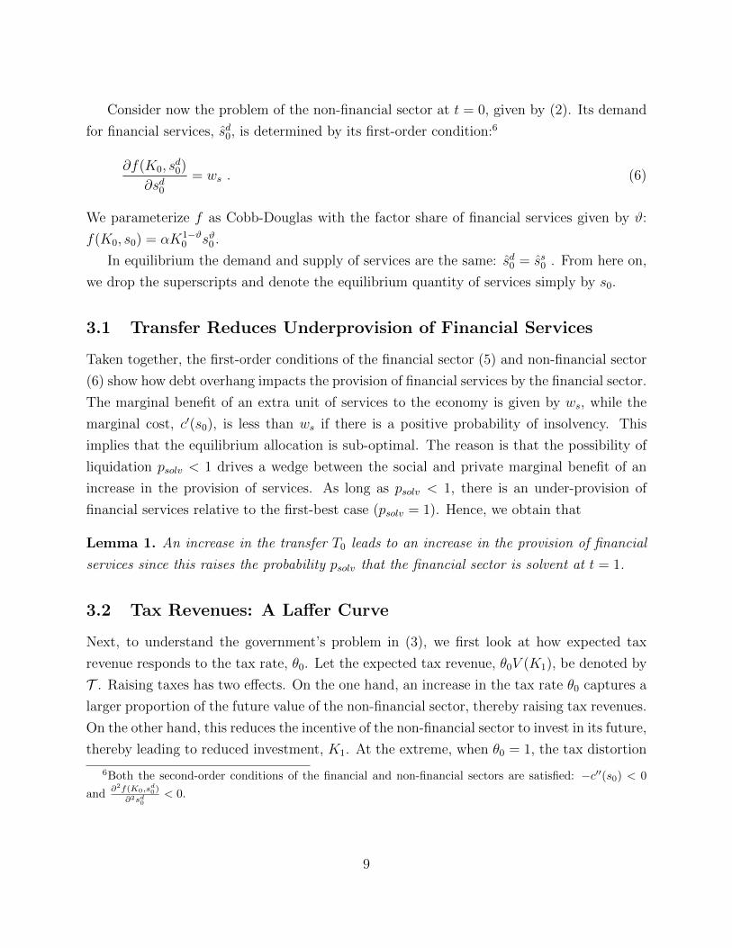
3.2 Tax Revenues: A Laffer Curve

Next, to understand the government’s problem in (3), we first look at how expected tax

revenue responds to the tax rate, θ0. Let the expected tax revenue, θ0V (K1), be denoted by

T . Raising taxes has two effects. On the one hand, an increase in the tax rate θ0 captures a

larger proportion of the future value of the non-financial sector, thereby raising tax revenues.

On the other hand, this reduces the incentive of the non-financial sector to invest in its future,

thereby leading to reduced investment, K1. At the extreme, when θ0 = 1, the tax distortion

6Both the second-order conditions of the financial and non-financial sectors are satisfied: −c′′(s0) < 0

and∂2f(K0,s

d0)

∂2sd0< 0.

9

eliminates the incentive for investment and tax revenues are reduced to zero. Hence, tax

revenues are non-monotonic in the tax rate and maximized by a tax rate strictly less than 1.

Formally, the impact on tax revenue of an increase in the tax rate is given by:

dTdθ0

= V (K1) + θ0V′(K1)

dK1

dθ0. (7)

Note that at θ0 = 0, an increase in the tax rate increases the tax revenue at a rate equal to

V (K1), the future value of the non-financial sector. It can be shown that since the production

function V (K1) is concave, as taxes are increased the incentive to invest is decreased by the

tax rate, that is dK1

dθ0< 0. To see this, consider the first-order condition for investment of the

non-financial sector at t = 1:

(1− θ0)V ′(K1)− 1 = 0 . (8)

Taking the derivative with respect to θ0 using the Implicit Function theorem gives: dK1

dθ0=

V ′(K1)(1−θ0)V ′′(K1)

< 0.7 Since at θ0 = 1 the tax revenue is zero this implies that the marginal

tax revenue decreases until it eventually becomes negative. Hence, tax revenues satisfy the

Laffer curve property as a function of the tax rate:

Lemma 2. The tax revenues, θ0V (K1), increase in the tax rate, θ0, as it increases from zero

(no taxes), and then eventually decline.

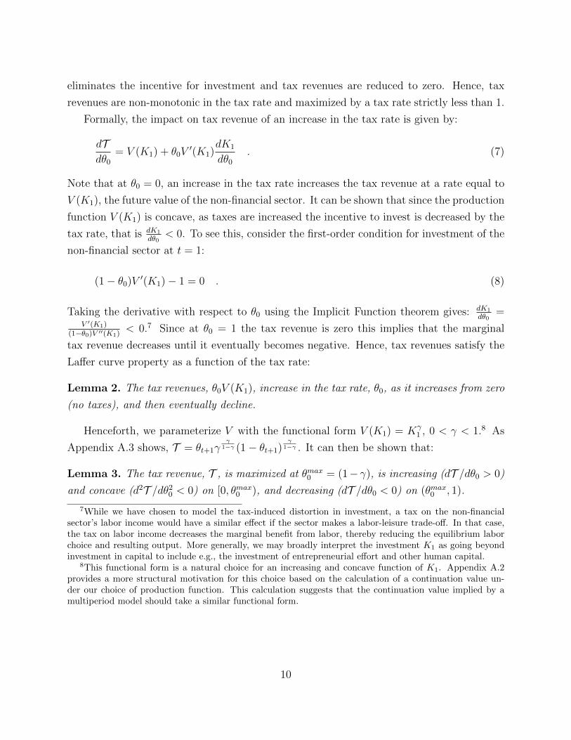
Henceforth, we parameterize V with the functional form V (K1) = Kγ1 , 0 < γ < 1.8 As

Appendix A.3 shows, T = θt+1γγ

1−γ (1− θt+1)γ

1−γ . It can then be shown that:

Lemma 3. The tax revenue, T , is maximized at θmax0 = (1− γ), is increasing (dT /dθ0 > 0)

and concave (d2T /dθ20 < 0) on [0, θmax0 ), and decreasing (dT /dθ0 < 0) on (θmax0 , 1).

7While we have chosen to model the tax-induced distortion in investment, a tax on the non-financialsector’s labor income would have a similar effect if the sector makes a labor-leisure trade-off. In that case,the tax on labor income decreases the marginal benefit from labor, thereby reducing the equilibrium laborchoice and resulting output. More generally, we may broadly interpret the investment K1 as going beyondinvestment in capital to include e.g., the investment of entrepreneurial effort and other human capital.

8This functional form is a natural choice for an increasing and concave function of K1. Appendix A.2provides a more structural motivation for this choice based on the calculation of a continuation value un-der our choice of production function. This calculation suggests that the continuation value implied by amultiperiod model should take a similar functional form.

10

3.3 Optimal Transfer Under Certainty and No Default

We analyze next the government’s decision starting first with a simplified version of the

general setup. We make two simplifying assumptions: (A1) we set to zero the variance of

the realized future value of the non-financial sector, so that V (K1) = V (K1); (A2) we force

the government to remain solvent. In subsequent sections we remove these assumptions.

If the government must remain solvent, it can only issue a number of bonds NT that it can

pay off in full, given its tax revenue. By assumption (A1), the tax revenue is known exactly

(it is equal to T ), and hence by assumption (A2), NT + ND = T . Moreover, since every

bond has a sure payoff of 1, we know that the bond price is P0 = 1. Then the transfer to the

financial sector is T0 = θ0V (K1) − ND and there is no probability of default, E[1def ] = 0.

Hence, the only choice variable for the government in this case is the tax rate. Appendix

A.4 shows that the first-order condition for the government can be expressed in terms of the

choice of transfer size (T0) and expected tax revenue (T ), rather than in terms of the tax

rate, and equates the marginal gain (G) and marginal loss (L) of increasing tax revenue:

dGdT

+dLdT

= 0 ,where (9)

dGdT

=∂f(K0, s0)

∂s0(1− psolv)

ds0dT0

, and

dLdT

= θ0V′(K1)

dK1

dT.

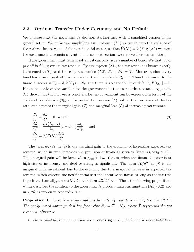
The term dG/dT in (9) is the marginal gain to the economy of increasing expected tax

revenue, which in turn increases the provision of financial services (since ds0/dT0 > 0) .

This marginal gain will be large when psolv is low, that is, when the financial sector is at

high risk of insolvency and debt overhang is significant. The term dL/dT in (9) is the

marginal underinvestment loss to the economy due to a marginal increase in expected tax

revenue, which distorts the non-financial sector’s incentive to invest as long as the tax rate

is positive. Formally, since dK1/dT < 0, then dL/dT < 0. Then, the following proposition,

which describes the solution to the government’s problem under assumptions (A1)-(A2) and

m ≥ 2ϑ, is proven in Appendix A.6:

Proposition 1. There is a unique optimal tax rate, θ0, which is strictly less than θmax0 .

The newly issued sovereign debt has face value NT = T − ND, where T represents the tax

revenues. Moreover,

1. The optimal tax rate and revenue are increasing in L1, the financial sector liabilities,

11

and in ND, the outstanding government debt.

2. The face value of newly issued sovereign debt (the transfer) is increasing in the fi-

nancial sector liabilities L1, but decreasing in the amount of existing government debt

ND. Moreover, the gross transfer, T0 + kAND, is also decreasing in ND.

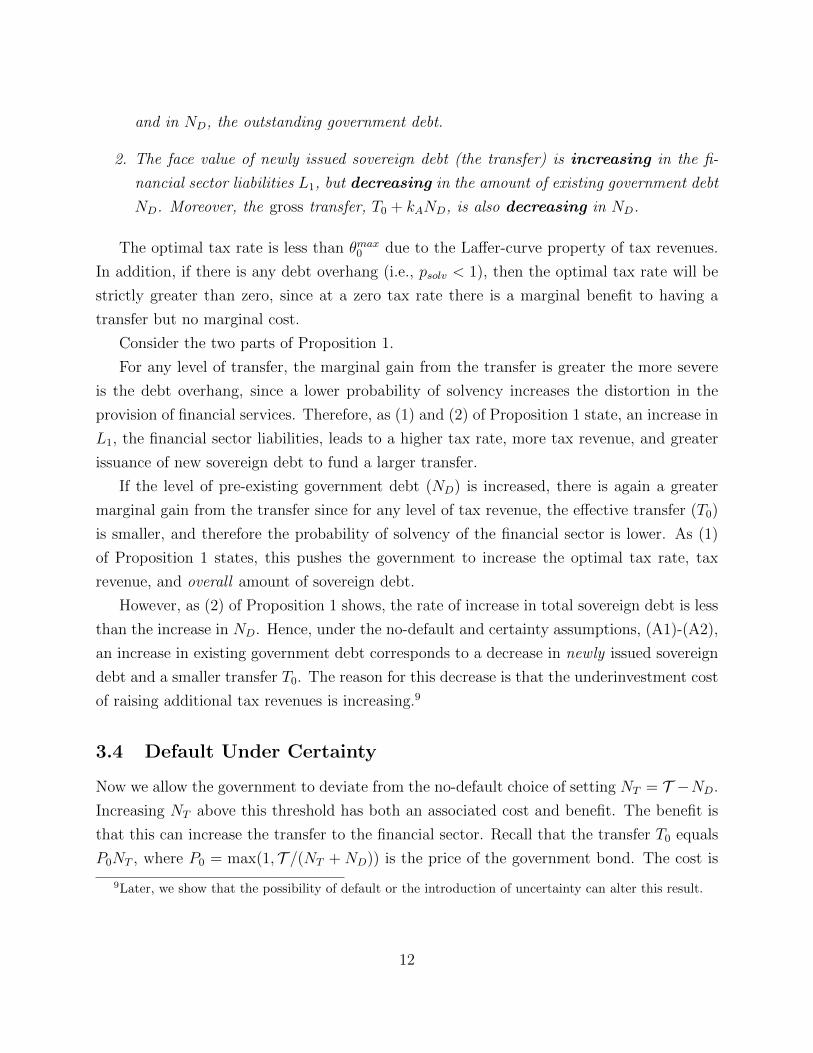
The optimal tax rate is less than θmax0 due to the Laffer-curve property of tax revenues.

In addition, if there is any debt overhang (i.e., psolv < 1), then the optimal tax rate will be

strictly greater than zero, since at a zero tax rate there is a marginal benefit to having a

transfer but no marginal cost.

Consider the two parts of Proposition 1.

For any level of transfer, the marginal gain from the transfer is greater the more severe

is the debt overhang, since a lower probability of solvency increases the distortion in the

provision of financial services. Therefore, as (1) and (2) of Proposition 1 state, an increase in

L1, the financial sector liabilities, leads to a higher tax rate, more tax revenue, and greater

issuance of new sovereign debt to fund a larger transfer.

If the level of pre-existing government debt (ND) is increased, there is again a greater

marginal gain from the transfer since for any level of tax revenue, the effective transfer (T0)

is smaller, and therefore the probability of solvency of the financial sector is lower. As (1)

of Proposition 1 states, this pushes the government to increase the optimal tax rate, tax

revenue, and overall amount of sovereign debt.

However, as (2) of Proposition 1 shows, the rate of increase in total sovereign debt is less

than the increase in ND. Hence, under the no-default and certainty assumptions, (A1)-(A2),

an increase in existing government debt corresponds to a decrease in newly issued sovereign

debt and a smaller transfer T0. The reason for this decrease is that the underinvestment cost

of raising additional tax revenues is increasing.9

3.4 Default Under Certainty

Now we allow the government to deviate from the no-default choice of setting NT = T −ND.

Increasing NT above this threshold has both an associated cost and benefit. The benefit is

that this can increase the transfer to the financial sector. Recall that the transfer T0 equals

P0NT , where P0 = max(1, T /(NT + ND)) is the price of the government bond. The cost is

9Later, we show that the possibility of default or the introduction of uncertainty can alter this result.

12

that when NT > T −ND, the government will not be able to fully cover its obligations. In

that case, P0 < 1 and the government will default, triggering the dead-weight loss of D.

Hence, the government’s decision on how many new bonds to issue, NT , splits the decision

space into two regions: (1) No Default: NT = T − ND and 1def = 0; and (2) Default:

NT > T −ND and 1def = 1.

As shown in Appendix A.7, if the choice to default is made, then it is optimal for the

government to issue an infinite amount of new debt in order to fully dilute existing debt (P0

becomes 0) and hence capture all tax revenues towards the transfer. The resulting situation

is the same as if existing debt ND had been set to zero. Therefore, to determine whether

defaulting is optimal, the government evaluates whether its objective function for given ND

and no default exceeds by at least D (the deadweight default cost) its objective function

with ND set to zero. Formally, let Wno def denote the maximum value of the government’s

objective function conditional on no default, Wdef denote the maximum value conditional on

default, and W = max(Wno def ,Wdef ). The following lemma, which is proved in Appendix

A.7, characterizes the optimal government action and resulting equilibrium:

Lemma 4. Conditional on default, it is optimal to set NT → ∞ (and hence P0 → 0).

This implies that Wdef = Wno def

∣∣ND=0

− D. Moreover, if default is undertaken then (1)

the optimal tax rate is lower, θdef0 < θno def0 ; (2) provided that kAND < T def , the gross

transfer is bigger, T0def

> T0no def

+ kAND; and, (3) equilibrium provision of financial

services is higher, s0def > s0

no def .

Figure 2 displays the optimal default boundary in L1 × ND space along with the No-

Default and Default regions. The following proposition characterizes how a number of factors

push the sovereign towards default, or in other words, move it closer to the default boundary.

Proposition 2. Ceteris paribus, the benefit to defaulting is:

1. increasing in the financial sector liabilities L1 (severity of debt overhang) and the

amount of existing government debt ND

2. decreasing in the dead-weight default cost D, and in the fraction of existing govern-

ment debt held by the financial sector kA.

Appendix A.8 provides the proof. Consider a worsening of the financial sector’s health,

leading to a decreased provision of financial services. This increases the marginal gain from

further government transfer, and, in turn, increases the gain to the sovereign from defaulting.

13

This is represented by a move towards the right in Figure 2, decreasing the distance to the

default boundary. An increase in existing debt implies a bigger spread between the optimal

transfer and tax revenue with and without default. Both the extra transfer and decreased

underinvestment represent benefits to defaulting. This is represented by a move upwards in

Figure 2, again decreasing the distance to the default-boundary.

It is clear that an increase in the deadweight loss raises the threshold for default.

Finally, and importantly, an increase in the fraction of existing sovereign debt held by

the financial sector also raises the threshold for default since the act of defaulting, which is

aimed at freeing up resources towards the transfer, causes collateral damage to the financial

sector balance sheet. From the vantage point of Figure 2, both an increase in D and kA

cause an outward shift in the default boundary.

3.4.1 Two-way Feedback

Propositions 1 and 2 indicate that there is a two-way feedback between the solvency situation

of the financial sector and of the sovereign. First, by Proposition 1, a severe deterioration

in the financial sector’s probability of solvency (e.g., an increase in L1) leads to a large

expansion in new debt (NT ) by the sovereign, as it acts to mitigate the under-provision

of financial services. Since the marginal cost of raising the tax revenue (dL/dT ) to fund

this debt expansion is increasing, the sovereign is pushed closer to the decision to default

(Proposition 2), as well as is its maximum debt capacity (Lemma 3). Hence, a financial

sector crisis pushes the sovereign towards distress.

Going in the other direction, by Proposition 1, a distressed sovereign, e.g., one with high

existing debt (ND), will have a financial sector with a worse solvency situation. This is

because it is very costly for such a sovereign to fund increased debt to make the transfer to

the financial sector. Hence, a more distressed sovereign will tend to correspond to a more

distressed financial sector (lower post-transfer psolv). Strategically defaulting is an avenue for

a distressed sovereign to free debt capacity for additional transfer. However, large holdings

of sovereign debt (kA) by the financial sector mean that taking this avenue simultaneously

causes collateral damage to the balance sheet of the financial sector, limiting the benefit

from this option (Proposition 2). In this case, a distressed sovereign is further incapacitated

in its ability to strengthen the solvency of its financial sector.

14

3.5 Uncertainty, Default, and Pricing

We now introduce uncertainty about future output (i.e., growth) by allowing the variance

of V (K1) to be nonzero. Instead of a binary default vs. no-default decision, the government

now implicitly chooses a continuous probability of default when it sets the tax rate and new

debt issuance. In this case, if raising taxes further incurs a large under-investment loss, the

government can choose to increase debt issuance while holding the tax rate constant. This

dilutes the claim of existing bondholders to tax revenues, thereby generating a larger transfer

without inducing further underinvestment. The trade-off is an increase in the government’s

probability of default and expected dead-weight default loss. In this case, the sovereign

effectively ‘sacrifices’ its own creditworthiness to improve the solvency of the financial sector,

leading to a ‘spillover’ of the financial sector crisis onto the credit risk of the sovereign.

Although θ0 and NT , are the variables the government directly chooses, it is more en-

lightening to look at two other variables that map one-to-one to them. The first variable is

T , which again equals θ0V (K1), the expected tax revenue. The second variable is:

H =NT +ND

T. (10)

In words, H is the ratio of outstanding debt to expected tax revenue. It is the sovereign’s

“insolvency ratio”, i.e. its ability to cover its total debt at face value. The government’s

problem (3) then is equivalent to optimally choosing T andH.10 Note that the no-default and

total-default cases under certainty correspond to setting H = 1 and H →∞, respectively.

To represent uncertainty we write V (K1) = V (K1)RV , where RV ≥ 0 represents the

shock to V (K1). By construction, E[RV ] = 1. We also assume that the distribution of RV

is independent of the variables K1, θ0, and NT .

Pricing, Default Probability and the Transfer: Using H we can easily express the

sovereign’s bond price, P0, and probability of default, pdef , as follows:

P0 = E0

[min

(1,θ0V (K1)

NT +ND

)]= E0

[min

(1,

1

HRV

)], (11)

pdef = prob(θ0V (K1) < NT +ND

)= prob

(RV < H

). (12)

10Formally, the mapping from θ0 to T is invertible on [0, θmax0 ] (as before, we can limit our concern to

this region) and given T , the mapping from H to NT is invertible. Hence, these alternative control variablesmap uniquely to the original ones on the region of interest.

15

Note that these quantities depend only on H and do not directly change with T . Next, as

NT = (T −ND/H)H, we can express the transfer in terms of T and H:

T0 = NTP0 = (T − ND

H)E0

[min

(H, RV

)]. (13)

The Optimal Probability of Default: Appendix A.9 and A.10 derive the first-order

conditions for T and H, respectively. The first-order condition for T , the expected tax

revenues, involves the same transfer-underinvestment trade-off as under certainty (adjusted

to account for H). Varying H, the sovereign’s insolvency ratio, involves a new trade-off.

Raising H increases the transfer by diluting existing bondholders–it raises outstanding debt

but without increasing expected tax revenue. This captures a greater faction of tax revenues

towards the transfer but raises the sovereign’s probability of default.

The top panel of Figure 3 illustrates the marginal gain (solid line) and loss (dashed

line) incurred by increasing H for a fixed level of T .11 The marginal cost of an increase

in H is the rise in expected dead-weight default cost. This is shown by the dashed green

line in Figure 3. Figure 3 indicates that (with T held constant) there are two potential

candidates for the optimal choice of H. The first is the value of H at which the gain and loss

curves intersect. The second is to let H →∞, representing a total default and full dilution

of existing bondholders. The bottom panel of Figure 3 plots the corresponding value of

the government’s objective as a function of H. The plot shows that for the configuration

displayed, a relatively small value of H achieves the optimum, which is at the intersection

of the gain and loss curves in the top panel. As this optimal H is above the lower end of

the support of RV (which is the origin in the figure), it corresponds to an optimal non-zero

probability of default. Note that above the upper end of the support of RV , the objective

function again rises in H, because once debt issuance is large enough that default is certain,

it is optimal for the government to fully dilute existing bondholders to obtain the largest

possible transfer. Finally, the dash-dot curves in Figure 3 show a case with an increase in

L1 (more severe debt overhang in the financial sector) relative to the solid lines.

3.5.1 Comparative Statics Under Uncertainty

The following proposition characterizes how different factors impact H and T , the govern-

ment’s optimal choices of H and T in equilibrium:

11To generate the plots we let RV have a uniform distribution.

16

Proposition 3. If (T , H) is an interior solution to the government’s problem on a region of

the parameter space, then the insolvency ratio H is increasing in the financial sector’s lia-

bilities L1, in the amount of existing government debt ND and decreasing in the deadweight

cost of default D. Furthermore, expected tax proceeds T are also increasing in L1.

Figure 4 plots comparative statics of the equilibrium (optimal) values of T , H, T0, and

P0 as L1 and ND are varied. The discontinuities that appears in the plots, as indicated by

the dotted lines, represent the point at which total default becomes optimal.

The top panel of Figure 4 varies L1. It shows that T increases in L1, up to the point where

the sovereign chooses total default. The corresponding plot for H tells a different story. For

low levels of L1, H is held constant at a low value. This value corresponds to the lower end

of the support of RV , so the probability of sovereign default remains 0. Correspondingly, the

plot shows that in this range, the bond price P0 remains fully valued at 1. For sufficiently

high L1 (e.g., financial crisis), the government chooses to increase H. It ‘sacrifices’ its own

creditworthiness in order to achieve a larger transfer. The increase in the transfer is apparent

in the subplot for T0, while the damage to the sovereign’s creditworthiness is apparent in the

plot for P0, which begins to decrease once H begins to rise.

The plots also show that when the financial sector’s situation is severe enough (L1 is

large), the optimal government response can be a total default, illustrated in the plots at

the point of the dotted line. As in the certainty case, total default fully dilutes existing

bondholders, freeing extra capacity for the sovereign to generate the transfer. This leads to

a jump up in T0 and a jump down in T . At the same time, P0 drops to 0.

The bottom panel of Figure 4 shows the comparative statics for ND. It is apparent that

for low levels of existing (i.e., pre-bailout) debt the sovereign keeps H constant at the low

end of its support, so there is no probability of default and P0 remains at 1. For these values

of ND, the government funds the transfer exclusively through increases in tax revenues. Note

that in this range the transfer is decreasing in ND, similar to the case of certainty. Once

ND is sufficiently high, the underinvestment costs of increasing tax revenue become so high

that the sovereign begins to increase H to fund the transfer. Consequently, the probability

of default rises and P0 begins to decrease, as shown in the plot. Interestingly, in this range

the combination of increased H and T imply that the transfer is actually increasing in ND.

The reason for this is that for large ND, the dilution of existing bondholders is an effective

channel for increasing the transfer. Moreover, as the plots show, at high enough ND, total

default becomes optimal.

17

3.6 Government ‘Guarantees’

We now consider a final extension. Explicit government guarantees of financial sector debt

have been a part of a number of countries’ financial sector bailouts, notably Ireland. More-

over, it has been common for sovereigns to step in to prevent the liquidation of banks by

guaranteeing their debt, which strongly suggests that there is an implicit ‘safety net’.12

To capture this, we add to the model a simple notion of a government guarantee of

financial sector debt. We do this for two reasons. First, guarantees are a measure that

serves to prevent liquidation of the financial sector by debtholders, which is a necessary

pre-condition for increasing the provision of financial services. Second, guarantees are rather

unique in that, by construction, their benefit is targeted at debt holders and not equity

holders. This unique feature is important in helping us identify empirically a direct feedback

between sovereign and financial sector credit risk. In the interest of simplicity, and since debt

overhang alleviation is the central feature of bailouts in the model, we do not explore the

feedback of the guarantees on the transfer and taxation decisions analyzed above. Instead,

we simply set the stage for implications of the guarantees for our empirical strategy.

3.6.1 Avoiding Liquidation

We model debtholders as potentially liquidating (or inducing a run on) the financial sector

if they are required to incur losses in case of financial sector default. To prevent debtholders

from liquidating, the government ‘guarantees’ their debt. That is, it pledges to bondholders

L1− A1−T0 from tax revenues in case of insolvency. The guarantee is pari-passu with other

claims on tax revenue. Hence, the guarantee has the same credit risk as other claims on the

sovereign. In fact, the guarantee is just equivalent to a claim that issues L1 − A1 − T0 new

government bonds to debt holders in case of insolvency.

Note that this claim accrues exclusively to debtholders and not to equityholders. This

differentiates it from general assets of the financial sector, such as the asset paying A1 or

the transfer, T0. Importantly, a change in the value of general assets of the firm changes

the value of equity and debt in a certain proportion, while a change in the value of the

guarantee changes the value of debt but not the value of equity. This implies that, if there

are guarantees, the change in equity value will not be sufficient for determining the change

in debt value. The following proposition gives a formal statement of this, derived under a

12The fallout from the failure of Lehman brothers and the apparent desire to prevent a repeat of thisexperience has strongly reinforced this view.

18

uniform distribution for A1 (same as used above to generate the figures).

Proposition 4. Let D be the value of debt, E the value of equity, and A1 ∼ U [Amin, Amax].

In the absence of a guarantee, the return on equity is sufficient for knowing the return on

debt. In contrast, in the presence of a guarantee, the return on debt is a bivariate function

of both the return on equity and the return on the sovereign bond price.

This bivariate dependence is approximated by the following relation:

dD

D≈ (1− psolv)(1− P0)

psolv

E

D

dE

E+

(1− psolv)2(Amax − Amin)

2

P0

D

dP0

P0

, (14)

which is derived in the Appendix A.13. The term involving the equity return (dEE

) captures

the impact on the debt value of any changes in the value of the general pool of assets of the

firm, including changes in the firm’s expected future profits. This type of result goes back

to Merton (1974), where the changes in both the debt and equity value reflect the change in

the total value of the firm. In the presence of a guarantee, there is an additional component,

which picks up the change in the value of debt coming from changes in the value of the

government guarantee. The change in value of the guarantee, which reflects variation in

the credit risk of the sovereign (dP0

P0), is concentrated primarily with debt and therefore not

captured adequately by the return on equity.

3.6.2 Two-way Feedback Revisited

Proposition 3 and Figure 4 show that with uncertainty about future output, the ‘spillover’

of the financial sector crisis onto the sovereign takes the form of a higher insolvency ratio H,

which is reflected in a lower sovereign bond price (and higher CDS rate). Once the insolvency

ratio H is increased, causing sovereign debt to become risky, negative shocks to sovereign

creditworthiness (e.g., shocks to growth and tax revenue RV ) then feed back onto the credit

risk of the financial sector by changing the value of its sovereign debt exposure– the transfer,

holdings of government bonds, and government guarantees. This feedback implies a post-

bailout increase in co-movement between sovereign and financial sector credit risk. This

increased co-movement contrasts with the immediate impact of the bailout announcement,

a reduction in financial sector credit risk and an increase in sovereign credit risk.

19

4 Empirics

In this section we present empirical evidence in favor of the main arguments formalized in

our model: (1) bank bailouts reduced financial sector credit risk but were a key factor in

triggering the rise in sovereign credit risk of the developed countries, and (2) there is a

two-way feedback between the credit risk of the sovereign and the financial sector.

The setting for our empirical analysis is the financial crisis of 2007-10. We divide the crisis

into three separate periods relative to the bailouts: pre, around, and after. The pre-bailout

period, which culminated in Lehman Brother’s bankruptcy, saw a severe deterioration in

banks’ balance sheets, a substantial rise in the credit risk of financial firms, and a significant

loss in the market value of bank equity. This negative shock generated substantial debt

overhang in the financial sector and significantly increased the likelihood of failure of, or

runs on, financial institutions. We interpret this as setting the stage for the initial time

period in the model, and the bank bailouts as the sovereign’s response, per the model.

We present our empirical results in two parts. The first part focuses on point (1). We

present evidence that the bailouts transmitted risk from the banks to the sovereigns and

triggered a rise in sovereign credit risk across a broad cross-section of developed countries.

We then confirm a prediction of the model by documenting the post-bailout emergence of a

positive relationship between sovereign credit risk and government debt-to-gdp ratios. We

also analyze the ability of the pre-bailout credit risk of the financial sector and the pre-bailout

government debt-to-gdp ratio to predict post-bailout sovereign credit risk. This relationship

is predicted by the model and is supportive of the argument that the bailouts led to the

emergence of sovereign credit risk in developed countries.

The second part of our analysis focuses on point (2) by testing for the sovereign-bank two-

way feedback. We use a broad panel of bank and sovereign CDS data to carry out tests that

establish this channel and show that it is quantitatively important. A significant challenge

in demonstrating direct sovereign-bank feedback is the concern that another (unobserved)

factor directly affects both bank and sovereign credit risk, giving rise to co-movement between

them even in the absence of any direct feedback. We address these concerns by utilizing a

particularly useful feature of government ‘guarantees’–that they are targeted specifically at

bank debt holders. This allows us to control for bank fundamentals using equity returns and

establish the direct sovereign-bank feedback.

We also gather data on the sovereign bond holdings of European banks that were released

after the stress tests conducted in the first half of 2010. Using these data we show that

20

bank holdings of foreign sovereign bonds have information about how sovereign credit risk

affects a bank’s credit risk. This result provides further evidence of a direct sovereign-to-

bank feedback because we control for country-specific macroeconomic changes by using the

change in value of foreign (rather than home) sovereign bonds.

We next describe the data construction and provide some summary statistics.

4.1 Data and Summary Statistics

We use Bankscope to identify all banks headquartered in Western Europe, the United States,

and Australia with more than $50 billion in assets as of the end of fiscal year 2006. We choose

this sample because smaller banks and banks outside these countries usually do not have

traded CDS. We then search for CDS in the database Datastream. We find CDS for 99

banks and match CDS to bank characteristics from Bankscope. Next, we search for equity

returns using Datastream. We find equity returns for 62 banks and match returns to CDS

and bank characteristics. Finally, we match these data to sovereign CDS (based on bank

headquarters) and OECD Economic Outlook data on public debt.

Panel A of Table 1 presents summary statistics for all banks with CDS prices. As of July

2007, the average bank had assets of $589.3 billion and equity of $26.8 billion. The average

equity ratio was 5.1% and the average Tier 1 ratio was 8.5%. The average bank CDS was

21.8 bps and the average sovereign CDS (if available as of July 2007) was 6.6 bps.

Panel B of Table 1 presents summary statistics of weekly changes in bank CDS and

sovereign CDS for the main bailout periods. We drop all observations with zero changes in

bank CDS or sovereign CDS to avoid stale data. All results presented below are robust to

including the dropped observations. Before the bank bailouts, the average bank CDS was

93.2 bps. The average sovereign CDS was only 13.5 bps, suggesting that financial market

participants did not anticipate large-scale bank bailouts prior to September 2008.

In the bailout period, we see a significant rise in both bank and sovereign credit risk with

average bank and sovereign CDS of 288.6 bps and 39.3 bps, respectively. Bank equity values

declined sharply during this period with a negative weekly return of 6.7%.

In the post-bailout period, average bank and sovereign CDS were 188.7 and 108.5 bps,

respectively. These CDS levels are suggestive of a significant transfer of financial sector

credit risk on sovereign balance sheets. We also find significant variation in sovereign CDS

with a standard deviation of weekly changes of 11.3%. This evidence suggests the emergence

of significant sovereign credit risk after the bank bailouts.

21

4.2 The Sovereign Risk Trigger

4.2.1 Bank and Sovereign CDS

The first bank bailout announcement in Western Europe was on September 30, 2008 in

Ireland. We define the pre-bailout period as starting on January 1, 2007 and ending on

September 26, 2008. We start the period in January 2007 to include the increase in bank

credit risk because of the financial crisis. Note that the pre-bailout period includes the

bankruptcy of Lehman Brothers on September 15, 2008 and the period immediately after-

wards, so that it includes the immediate effect of Lehman’s bankruptcy on other banks.

Hence, the pre-bailout period captures both the prolonged increase in bank credit risk dur-

ing 2007-2008 and the post-Lehman spike that occurs before the bank bailouts. To examine

bank and sovereign credit risk in this period, we analyze the country-level change in sovereign

and bank CDS. For each country, we compute the change in bank CDS as the unweighted

average of all banks with traded CDS.

Figure 5 summarizes the results for the pre-bailout period. For each country, the first

column depicts the change in sovereign CDS and the second column depicts the change in

bank CDS over the pre-bailout period. The figure shows that there is a large increase in

bank CDS during this period. For example, the average bank CDS in Ireland increased by

300 bps. However, there was almost no change in Ireland’s sovereign CDS. Overall, the figure

shows that the credit risk of the financial sector was greatly increased over the pre-bailout

period but that there was little impact on sovereign credit risk.13

Within one month after the Irish bailout was announced on September 30, 2008, almost

every Western European country announced a bank bailout. The bailouts typically consisted

of asset purchase programs, debt guarantees, and equity injections or some combination

thereof. The programs were substantial with estimated costs of 54% of GDP in Great

Britain, 28% of GDP in Germany, and 22% of GDP in the United States (Panetta et al.

(2009)). Several countries made more than one announcement during this period. Many

countries followed Ireland’s example in part to offset outflows from their own financial sectors

to newly secured financial sectors. As a result, the bank bailout announcements were not

truly independent. We therefore define the bailout period as the one-month period in which

13We note that some investors may have expected bank bailouts even before the first official announcementon September 30, 2008. Such an expectation would reduce the observed increase in bank CDS and shiftforward in time the rise in sovereign CDS. To the extent that investors held such expectations prior toSeptember 30, 2008, they can explain the small rise in sovereign CDS that occurs late in the pre-bailoutperiod. However, the fact that the impact in this period is so small quantitatively suggest that the bankbailouts were a surprise to the majority of investors.

22

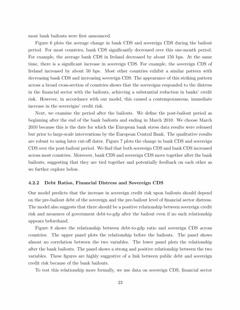
most bank bailouts were first announced.

Figure 6 plots the average change in bank CDS and sovereign CDS during the bailout

period. For most countries, bank CDS significantly decreased over this one-month period.

For example, the average bank CDS in Ireland decreased by about 150 bps. At the same

time, there is a significant increase in sovereign CDS. For example, the sovereign CDS of

Ireland increased by about 50 bps. Most other countries exhibit a similar pattern with

decreasing bank CDS and increasing sovereign CDS. The appearance of this striking pattern

across a broad cross-section of countries shows that the sovereigns responded to the distress

in the financial sector with the bailouts, achieving a substantial reduction in banks’ credit

risk. However, in accordance with our model, this caused a contemporaneous, immediate

increase in the sovereigns’ credit risk.

Next, we examine the period after the bailouts. We define the post-bailout period as

beginning after the end of the bank bailouts and ending in March 2010. We choose March

2010 because this is the date for which the European bank stress data results were released

but prior to large-scale interventions by the European Central Bank. The qualitative results

are robust to using later cut-off dates. Figure 7 plots the change in bank CDS and sovereign

CDS over the post-bailout period. We find that both sovereign CDS and bank CDS increased

across most countries. Moreover, bank CDS and sovereign CDS move together after the bank

bailouts, suggesting that they are tied together and potentially feedback on each other as

we further explore below.

4.2.2 Debt Ratios, Financial Distress and Sovereign CDS

Our model predicts that the increase in sovereign credit risk upon bailouts should depend

on the pre-bailout debt of the sovereign and the pre-bailout level of financial sector distress.

The model also suggests that there should be a positive relationship between sovereign credit

risk and measures of government debt-to-gdp after the bailout even if no such relationship

appears beforehand.

Figure 8 shows the relationship between debt-to-gdp ratio and sovereign CDS across

countries. The upper panel plots the relationship before the bailouts. The panel shows

almost no correlation between the two variables. The lower panel plots the relationship

after the bank bailouts. The panel shows a strong and positive relationship between the two

variables. These figures are highly suggestive of a link between public debt and sovereign

credit risk because of the bank bailouts.

To test this relationship more formally, we use data on sovereign CDS, financial sector

23

distress, and government debt-to-gdp ratios. We measure pre-bailout financial sector distress

at the country level by averaging bank CDS on September 22, 2008. We choose this date

midway between Lehman’s bankruptcy and the first bailout announcement. We measure the

government debt-to-gdp ratio as the government gross liabilities as a percentage of gdp in

the year before the bailouts. For the post-bailout date we again choose March 31, 2010, the

reporting date for the European bank stress tests. We estimate the following regression:

yi = α + β(Pre-Bailout Debti) + γ log(Financial Sector Distressi) + εi

where the outcome variable yi is either the natural logarithm of sovereign CDS or the debt-

to-gdp ratio of country i.

Table 2 presents the result of our analysis. We first focus on the post-bailout results.

Column (3) finds that a 1% increase in the pre-bailout debt-to-gdp ratio leads to a 1.5%

increase in sovereign CDS post-bailout.14 Column (4) shows that a 1% increase in pre-bailout

financial sector distress increases post-bailout sovereign CDS by 0.965%. The coefficient on

debt-to-gdp decreases slightly but remains marginally significant. The R-squared of the

regression is close to 50%. These results suggest that pre-bailout financial sector distress

and sovereign’s debt-to-gdp ratio are highly predictive of post-bailout sovereign credit risk.

In contrast, Column (1) of Table 2 shows that in the pre-bailout period there is only a

very weak relationship between debt-to-gdp and sovereign CDS. The coefficient is small and

statistically insignificant. Column (2) shows that the coefficient on financial sector distress

in the pre-bailout period is also statistically insignificant.

From these results we can see that there emerged a relationship between debt-to-gdp and

sovereign credit risk that was not present beforehand. Note, moreover, that the emergence of

this relationship coincides with an overall rise in sovereign debt ratios. In the context of our

model, the sovereigns have raised their insolvency ratios H, so that dilution of existing debt

occurs, and there emerges a negative relationship between debt-to-gdp and the government

bond price (see Figure 4).

Column (5) examines the ability of pre-bailout financial sector distress to predict the

change in government debt-to-gdp from the pre-bailout to the post-bailout period. Consis-

14We make note of two points. First, the model predicts that the insolvency ratio H determines the levelof sovereign CDS. However, the debt-to-gdp ratio corresponds to θ0H in the model rather than simply H.Nevertheless, the prediction of the model carries over to θ0H since θ0 is increasing in financial sector distress.Second, debt-to-gdp ratios are an imperfect proxy for θ0H because H takes into account any future issuanceof debt to pay for current obligations related to the bailouts, whereas debt-to-gdp ratios are lagging. Wecan address this to some extent by using the leading debt-to-gdp ratio.

24

tent with the model, we find that financial sector distress is positively related to the increase

in debt-to-gdp. The coefficient is positive and marginally statistically significant. Column

(6) shows that post-bailout debt-to-gdp is predicted by pre-bailout debt-to-gdp and pre-

bailout financial sector distress. Both coefficients are statistically significant and together

the two variables explain 84% of the variation in post-bailout debt-to-gdp.

4.3 The Sovereign-Bank Feedback

This section analyzes the two-way feedback between sovereign and bank sector credit risk.

Once the sovereign opens itself up to credit risk due to bailouts, the price of its debt becomes

sensitive to macroeconomic shocks. Moreover, our model indicates that subsequent changes

in the sovereign’s credit risk should impact the financial sector’s credit risk through three

channels: (i) ongoing bailout payments and subsidies, (ii) direct holdings of government

debt, and (iii) explicit and implicit government guarantees. In our empirical analysis, we

estimate the aggregate effect of these three channels.

We start by estimating the following relationship in the post-bailout period:

∆ log(Bank CDSijt) = α + β∆ log(Sovereign CDSjt) + εijt

where ∆ log(Bank CDSijt) is the change in the log CDS of bank i headquartered in country

j from time t to time t − 1 and ∆ log(Sovereign CDSjt) is the change in the log Sovereign

CDS of country j from time t to time t − 1. At the weekly frequency, in the post-bailout

period the estimate of β is 0.47 and highly statistically signficant. This means that a 10%

increase in sovereign CDS is associated with a 4.7% increase in bank CDS. This result is

consistent with direct sovereign-to-bank feedback.

However, an obvious concern is that there is another (unobserved) factor that affects

both bank and sovereign credit risk. Such a factor could explain the co-movement without

there necessarily being an underlying direct channel between sovereign and bank credit risk.

More specifically, we interpret changes in sovereign credit risk as changes in expectations

about macroeconomic fundamentals, such as employment, growth, and productivity. These

fundamentals also have a direct effect on the value of bank assets such as mortgages or

bank loans. Hence, changes in macroeconomic conditions may generate a correlation be-

tween sovereign and bank credit risk even in the absence of the direct feedback mechanism.

Therefore, establishing that there is a direct feedback between sovereign and financial sector

credit risk is a significant empirical challenge.

25

We use several strategies to address this concern. Our first strategy is to include three

sets of controls. First, we add controls that capture market-wide changes that affect both

bank and sovereign risk directly. Our market-wide controls are a CDS-market index and a

measure of aggregate volatility. Our CDS market index is the iTraxx Europe index, which is

comprised of 125 of the most liquid CDS names referencing European investment grade cred-

its. The CDS market index captures market-wide variation in CDS rates caused by changes

in fundamental credit risk, liquidity, and CDS-market specific shocks.15 For the volatility

index we follow the empirical literature and use a VIX-like index, the VDAX, which is the

German counterpart to the VIX index for the S&P 500. This captures changes in aggregate

volatility, which is an important factor in the pricing of credit risk. Second, we include

weekly fixed effects. The fixed effects captures (unobserved) variation that is common across

all banks. Third, we include bank-specific coefficients on all the control variables and bank

fixed effects. This accommodates potential non-linearities in the estimated relationships.

We implement this approach by estimating the following regression:

∆ log(Bank CDSijt) = αi + δt + β∆ log(Sovereign CDSjt) + γ∆Xijt + εijt

where ∆Xijt are the changes in the control variables from time t to time t− 1, δt are weekly

fixed effects, and αi are bank fixed-effects.

Table 3 shows the results for the pre-, around, and post-bailout period. For each period

there are three columns of results. The left column reports the coefficient after including the

market-wide control variables. The middle column adds the weekly fixed effects. The right

column adds bank fixed effects and bank-specific coefficients on controls.

Our main focus is on testing for the sovereign-to-bank feedback, so we examine the post-

bailout results first. Column (7) shows that β is positive, as expected, and highly statistically

significant. The magnitude is also economically important, implying that an increase in

sovereign CDS of 10% translates into a 2.21% increase in bank CDS. The control coefficients

are both statistically significant and the signs are as expected; an increase in aggregate CDS

levels or aggregate volatility is associated with a rise in bank CDS. Altogether, the variables

explain 33.8% of the variation in weekly bank CDS.

Column (8) adds the weekly fixed effects. The coefficient on sovereign CDS decreases but

15Collin-Dufresne, Goldstein, and Martin (2001) find that a substantial part of the variation in corporatecredit spread changes is driven by a single factor that is independent of changes in risk factors or measuresof liquidity. They therefore conclude that this variation represents ‘local supply/demand shocks’ in thecorporate bond market.

26

remains highly statistically significant. The decrease is not surprising, as time fixed effects

represent a rich set of controls. The weekly fixed effects are collinear with the market-wide

control variables; therefore, we do not estimate coefficients on the market-wide controls.

There is an increase in the R-squared of about 7.6% over column (7), indicating that most

of the unobserved market-wide variation was already captured by the market-wide controls.

Column (9) shows that the coefficient on sovereign CDS is essentially unchanged and

remains highly statistically significant after adding bank-specific coefficients on the market-

wide control variables. Given the flexibility of this specification, we interpret the coefficients

on sovereign CDS as robust evidence in favor of direct sovereign-to-bank feedback.

Comparing these results with those for the around-bailout period in columns (4)-(6) shows

interesting differences. For the around-bailout period, the coefficient on sovereign CDS is

negative after controlling for week fixed effects. In other words, in the around-bailout period

an increase in sovereign CDS is associated with a decrease in bank CDS. This is consistent

with the evidence for bank-to-sovereign feedback that the sovereigns took onto themselves

credit risk from their financial sectors during this phase. As shown in Column (6), the

coefficient is large and statistically significant with a 10% increase in sovereign CDS leading

to 12.9% decrease in bank CDS.

Columns (1)-(3) show the results for the pre-bailout period. They show small coefficients

on sovereign CDS that are indistinguishable from zero. As expected, in the pre-bailout

period there is no evidence for sovereign-bank feedbacks. In contrast, the CDS market

control coefficient is significant and has a large magnitude, as for the other periods.

We also provide a non-parametric illustration of this result. We add interactions of

month fixed-effects and sovereign CDS to the regression model describe above (including all

controls). Figure 9 plots the three-month moving average and the 95%-confidence interval of

the coefficients on the interactions.16 As shown in the figure, in the pre-bailout period there

is a a zero correlation (with relatively tight standard errors) between bank and sovereign

CDS. During the bailout period, the correlation turns negative and is highly statistically

significant with a coefficient of -0.3. After the bailout period, the coefficient is positive and

mostly statistically significant with a coefficient of around 0.12. This result lends further

support to our analysis of three distinct bailout periods.

16We construct the standard errors based on the estimated standard errors of the month fixed-effectsassuming a zero correlation of error terms across months.

27

4.3.1 Controlling for Bank Fundamentals

The results above establish that there is a strong two-way sovereign-bank feedback. However,

there may remain a concern that our strategy to this point does not control for country-

specific macroeconomic shocks that affect both sovereign and credit risk. These shocks may

not be fully captured by our market-wide controls if they have a heterogenous impact across

countries.

We address this concern by employing a strategy that utilizes a particularly useful feature

of bank bailouts. Specifically, most bailouts were partly structured in the form of govern-

ment ‘guarantees’, which are targeted specifically at bank debt holders. This implies that

sovereign-specific shocks should have a disproportionate impact on debt holders because, in

addition to changing the value of bank assets, such shocks change the value of government

‘guarantees’ (implicit or explicit). Therefore, to establish whether there is direct sovereign-

to-bank feedback, we can test if sovereign CDS is a determinant of bank CDS even after we

control for the impact of shocks to bank fundamentals.

This empirical strategy is motivated by our guarantees model (Section 3.6), which shows

that bank equity returns are sufficient for determining changes in bank CDS in the absence

of government ‘guarantees’.17 This implies that once we control for bank equity returns

we should not find that changes in sovereign CDS have any further explanatory power for

changes in bank CDS. However, if one finds that sovereign CDS does have further explanatory

power for bank CDS beyond equity returns, then this is strongly supportive of a sovereign-

to-bank feedback channel. Proposition 4 shows that ‘guarantees’ present a source for such a

potential finding because they discriminate precisely in favor of debtholders. In the presence

of ‘guarantees’, a projection of changes in bank CDS that controls for equity returns should

still find a (positive) exposure on changes in sovereign CDS.

We therefore augment the regression with banks’ weekly equity returns. The estimates

are shown in Table 4. The structure is similar to Table 3. Columns (7)-(9) show that in

the post-bailout period the coefficient on sovereign CDS survives and is highly statistically

significant. As shown in columns (7) and (8), although the bank stock return coefficient

is highly statistically significant and possesses the expected negative sign, its inclusion has

little impact on the magnitude of the sovereign CDS coefficient. Column (9) includes bank-

specific coefficients on bank stock returns. The results show that the coefficient on sovereign

17This result is in fact quite general. It holds in models of defaultable bond pricing that build on thecanonical model of Merton (1974), where stock returns contain all information about changes in bank assetvalues and therefore can (locally) capture all variation in the price of debt.

28

CDS decreases somewhat but remains highly significant. We note that the coefficients in

Column (7) to (9) are slightly smaller than the comparable coefficients in Table 3. This is

consistent with small, positive benefits of bank bailouts to bank equity holders.18

For the bailout and pre-bailout periods, the results are quite similar to those in Table 3.

As shown in columns (1) to (6), we again find a negative coefficient on sovereign CDS in the

bailout period and an essentially zero coefficient in the pre-bailout period.

4.3.2 Bank-level Heterogeneity

To analyze further the sovereign-to-bank feedback, we also examine whether heterogeneity in

bank- and country-level characteristics affects banks’ sensitivity to changes in sovereign CDS

during the post-bailout period. To this end, we estimate the coefficient on an interaction

term of changes in sovereign CDS with bank and country-level variables.

We examine three variables. The first variable is the Tier 1 capital ratio, which is

commonly used in the banking industry as a proxy for a bank’s probability of solvency. This

specification is motivated by our theoretical result that the impact of changes in the value

of government guarantees should be stronger for less well-capitalized banks. We measure

Tier 1 capital ratio before the bailouts (as of January 2007) to avoid endogenous changes in

this variable as the result of bailouts. The second variable is the share of liabilities financed

with short-term debt (as of January 2007 from Bankscope). This variable captures a bank’s

need to roll over funding within less than a year. Intuitively, the impact of changes in the

value of government guarantees should be stronger for banks with larger short-term funding

needs. Again, we measure the variable as of January 2007. The third variable is the level of

sovereign credit risk. The impact of changes in the value of government guarantees should

be stronger for more risky sovereigns. Given that sovereign credit risk arose as a result of

the bailouts, we measure this variable using the natural logarithm of sovereign CDS lagged

by 12 weeks.

Table 5 reports the results. The coefficient of interest is the interaction term. Columns (1)

and (3) find that banks with higher Tier 1 ratios were less sensitive to variation in sovereign

18For the purposes of establishing the existence of a two-way feedback, we mainly focus on changes in bankCDS. It is also interesting to look at the impact of bailouts on bank equity returns. From the viewpoint ofthe model, bank equity returns should reflect changes in sovereign credit risk due to their impact on the valueof continuing bailout payments and banks’ holdings of government bonds. To that end, we also estimated allour benchmark regression from Table 3 with equity returns as outcome variable. Indeed, we find a similarrelationship for bank equity returns as we find for bank CDS in Table 3 (as expected, the coefficient in thepost-bailout period has the opposite sign because a rise in sovereign CDS reduces equity returns). Thisfinding supports our assumption that equity returns are a suitable control for changes in bank fundamentals.

29

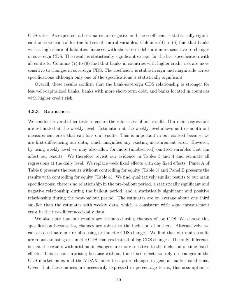
CDS rates. As expected, all estimates are negative and the coefficient is statistically signifi-

cant once we control for the full set of control variables. Columns (4) to (6) find that banks

with a high share of liabilities financed with short-term debt are more sensitive to changes

in sovereign CDS. The result is statistically significant except for the last specification with

all controls. Columns (7) to (9) find that banks in countries with higher credit risk are more

sensitive to changes in sovereign CDS. The coefficient is stable in sign and magnitude across

specifications although only one of the specifications is statistically significant.

Overall, these results confirm that the bank-sovereign CDS relationship is stronger for

less well-capitalized banks, banks with more short-term debt, and banks located in countries

with higher credit risk.

4.3.3 Robustness

We conduct several other tests to ensure the robustness of our results. Our main regressions

are estimated at the weekly level. Estimation at the weekly level allows us to smooth out

measurement error that can bias our results. This is important in our context because we

are first-differencing our data, which magnifies any existing measurement error. However,

by using weekly level we may also allow for more (unobserved) omitted variables that can

affect our results. We therefore revisit our evidence in Tables 3 and 4 and estimate all

regressions at the daily level. We replace week fixed effects with day fixed effects. Panel A of

Table 6 presents the results without controlling for equity (Table 3) and Panel B presents the

results with controlling for equity (Table 4). We find qualitatively similar results to our main

specifications: there is no relationship in the pre-bailout period, a statistically significant and

negative relationship during the bailout period, and a statistically significant and positive

relationship during the post-bailout period. The estimates are on average about one third

smaller than the estimates with weekly data, which is consistent with some measurement

error in the first-differenced daily data.

We also note that our results are estimated using changes of log CDS. We choose this

specification because log changes are robust to the inclusion of outliers. Alternatively, we

can also estimate our results using arithmetic CDS changes. We find that our main results

are robust to using arithmetic CDS changes instead of log CDS changes. The only difference

is that the results with arithmetic changes are more sensitive to the inclusion of time fixed-

effects. This is not surprising because without time fixed-effects we rely on changes in the

CDS market index and the VDAX index to capture changes in general market conditions.

Given that these indices are necessarily expressed in percentage terms, this assumption is

30

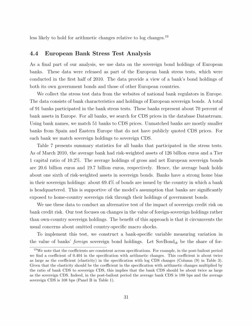
less likely to hold for arithmetic changes relative to log changes.19

4.4 European Bank Stress Test Analysis

As a final part of our analysis, we use data on the sovereign bond holdings of European

banks. These data were released as part of the European bank stress tests, which were

conducted in the first half of 2010. The data provide a view of a bank’s bond holdings of

both its own government bonds and those of other European countries.

We collect the stress test data from the websites of national bank regulators in Europe.

The data consists of bank characteristics and holdings of European sovereign bonds. A total

of 91 banks participated in the bank stress tests. These banks represent about 70 percent of

bank assets in Europe. For all banks, we search for CDS prices in the database Datastream.

Using bank names, we match 51 banks to CDS prices. Unmatched banks are mostly smaller

banks from Spain and Eastern Europe that do not have publicly quoted CDS prices. For

each bank we match sovereign holdings to sovereign CDS.

Table 7 presents summary statistics for all banks that participated in the stress tests.

As of March 2010, the average bank had risk-weighted assets of 126 billion euros and a Tier

1 capital ratio of 10.2%. The average holdings of gross and net European sovereign bonds

are 20.6 billion euros and 19.7 billion euros, respectively. Hence, the average bank holds

about one sixth of risk-weighted assets in sovereign bonds. Banks have a strong home bias

in their sovereign holdings: about 69.4% of bonds are issued by the country in which a bank

is headquartered. This is supportive of the model’s assumption that banks are significantly

exposed to home-country sovereign risk through their holdings of government bonds.

We use these data to conduct an alternative test of the impact of sovereign credit risk on

bank credit risk. Our test focuses on changes in the value of foreign-sovereign holdings rather

than own-country sovereign holdings. The benefit of this approach is that it circumvents the

usual concerns about omitted country-specific macro shocks.

To implement this test, we construct a bank-specific variable measuring variation in

the value of banks’ foreign sovereign bond holdings. Let SovBondik be the share of for-

19We note that the coefficients are consistent across specifications. For example, in the post-bailout periodwe find a coefficient of 0.404 in the specification with arithmetic changes. This coefficient is about twiceas large as the coefficient (elasticity) in the specification with log CDS changes (Column (9) in Table 3).Given that the elasticity should be the coefficient in the specification with arithmetic changes multiplied bythe ratio of bank CDS to sovereign CDS, this implies that the bank CDS should be about twice as largeas the sovereign CDS. Indeed, in the post-bailout period the average bank CDS is 188 bps and the averagesovereign CDS is 108 bps (Panel B in Table 1).

31

eign sovereign holdings of country k by bank i. We calculate the foreign holdings variable,

ForeignBondCDSit as the following weighted average:

ForeignBondCDSit =∑i 6=j

SovBondik ∗ SovereignCDSkt

where SovereignCDSkt is the sovereign CDS of country k on day t. Note that for each bank

the foreign holdings variable excludes home-sovereign bonds. We then estimate the following:

∆ log(Bank CDSit) = δt + γ∆ log(ForeignBondCDSit) + εit (15)

where δt are time fixed effects. The coefficient of interest is γ, which captures the effect of

changes in the value of foreign bond holdings on bank CDS. We estimate the regressions

using the period one month before and one month after the reporting date for the sovereign

bond holdings. By estimating this regression, we are implicitly assuming that the marginal

CDS investor either knows or at least has some idea of the bank holdings.

Table 8 shows the results. Column (1) shows a positive and statistically significant asso-

ciation between changes in bank CDS and their foreign sovereign holdings. This coefficient

suggests that a one-standard deviation increase in the change in the foreign sovereign hold-

ings variable leads to an increase of about half of a one-standard deviation in the change of

the bank CDS. Column (2) shows that the coefficient remains unchanged when bank fixed

effects are included. Column (3) controls for week fixed effects. The coefficient of inter-

est decreases by about one third but remains statistically significant. This suggests that

common shocks affect both the change in bank CDS and the change in the foreign holdings

variable. Column (4) controls for day fixed effects. The coefficient decreases by two third

relative to the specification without time fixed effects but remains statistically significant

at the 1%-level. This result suggests that variation in foreign sovereign holdings contains

economically important information about variation in bank credit risk.

To further check for robustness, column (5) adds bank fixed effects in addition to day fixed

effects. This does not have any effect on the coefficient of interest. Column (6) estimates

the same regression as in Column (5) but excludes the holdings of German bonds from the

construction of the foreign-holdings variable. We do this to address a potential concern

about reverse causality due to the possibility that Germany may provide bailouts to other

countries, or banks in other countries. The column shows that this has no effect on the

coefficient of interest.

32

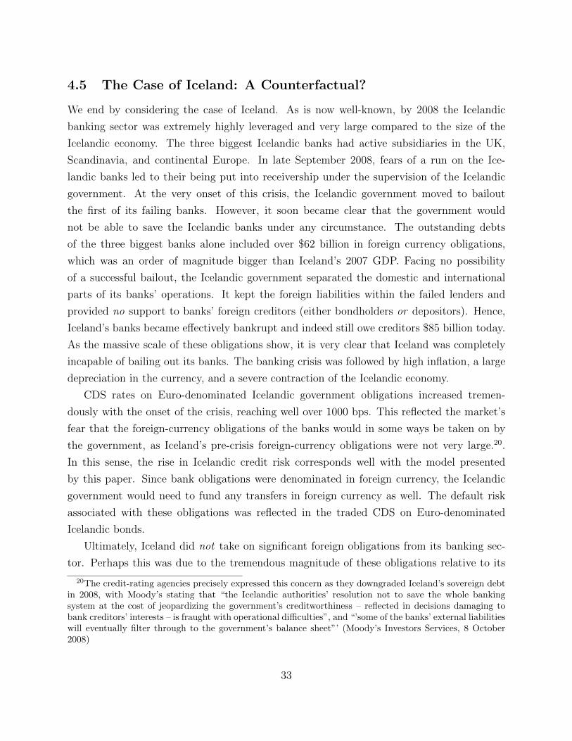
4.5 The Case of Iceland: A Counterfactual?

We end by considering the case of Iceland. As is now well-known, by 2008 the Icelandic

banking sector was extremely highly leveraged and very large compared to the size of the

Icelandic economy. The three biggest Icelandic banks had active subsidiaries in the UK,

Scandinavia, and continental Europe. In late September 2008, fears of a run on the Ice-

landic banks led to their being put into receivership under the supervision of the Icelandic

government. At the very onset of this crisis, the Icelandic government moved to bailout

the first of its failing banks. However, it soon became clear that the government would

not be able to save the Icelandic banks under any circumstance. The outstanding debts

of the three biggest banks alone included over $62 billion in foreign currency obligations,

which was an order of magnitude bigger than Iceland’s 2007 GDP. Facing no possibility

of a successful bailout, the Icelandic government separated the domestic and international

parts of its banks’ operations. It kept the foreign liabilities within the failed lenders and

provided no support to banks’ foreign creditors (either bondholders or depositors). Hence,

Iceland’s banks became effectively bankrupt and indeed still owe creditors $85 billion today.

As the massive scale of these obligations show, it is very clear that Iceland was completely

incapable of bailing out its banks. The banking crisis was followed by high inflation, a large

depreciation in the currency, and a severe contraction of the Icelandic economy.

CDS rates on Euro-denominated Icelandic government obligations increased tremen-

dously with the onset of the crisis, reaching well over 1000 bps. This reflected the market’s

fear that the foreign-currency obligations of the banks would in some ways be taken on by

the government, as Iceland’s pre-crisis foreign-currency obligations were not very large.20.

In this sense, the rise in Icelandic credit risk corresponds well with the model presented

by this paper. Since bank obligations were denominated in foreign currency, the Icelandic

government would need to fund any transfers in foreign currency as well. The default risk

associated with these obligations was reflected in the traded CDS on Euro-denominated

Icelandic bonds.

Ultimately, Iceland did not take on significant foreign obligations from its banking sec-

tor. Perhaps this was due to the tremendous magnitude of these obligations relative to its

20The credit-rating agencies precisely expressed this concern as they downgraded Iceland’s sovereign debtin 2008, with Moody’s stating that “the Icelandic authorities’ resolution not to save the whole bankingsystem at the cost of jeopardizing the government’s creditworthiness – reflected in decisions damaging tobank creditors’ interests – is fraught with operational difficulties”, and “’some of the banks’ external liabilitieswill eventually filter through to the government’s balance sheet”’ (Moody’s Investors Services, 8 October2008)

33

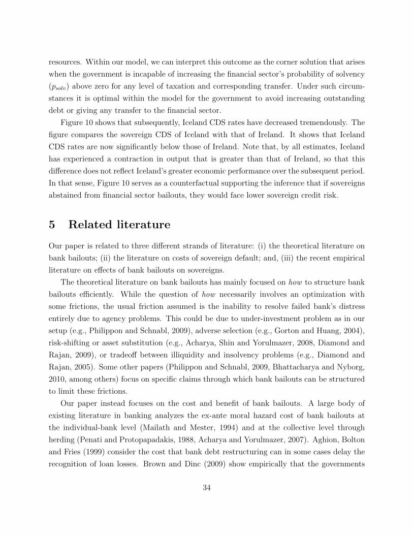
resources. Within our model, we can interpret this outcome as the corner solution that arises

when the government is incapable of increasing the financial sector’s probability of solvency

(psolv) above zero for any level of taxation and corresponding transfer. Under such circum-

stances it is optimal within the model for the government to avoid increasing outstanding

debt or giving any transfer to the financial sector.

Figure 10 shows that subsequently, Iceland CDS rates have decreased tremendously. The

figure compares the sovereign CDS of Iceland with that of Ireland. It shows that Iceland

CDS rates are now significantly below those of Ireland. Note that, by all estimates, Iceland

has experienced a contraction in output that is greater than that of Ireland, so that this

difference does not reflect Iceland’s greater economic performance over the subsequent period.

In that sense, Figure 10 serves as a counterfactual supporting the inference that if sovereigns

abstained from financial sector bailouts, they would face lower sovereign credit risk.

5 Related literature

Our paper is related to three different strands of literature: (i) the theoretical literature on

bank bailouts; (ii) the literature on costs of sovereign default; and, (iii) the recent empirical

literature on effects of bank bailouts on sovereigns.

The theoretical literature on bank bailouts has mainly focused on how to structure bank

bailouts efficiently. While the question of how necessarily involves an optimization with

some frictions, the usual friction assumed is the inability to resolve failed bank’s distress

entirely due to agency problems. This could be due to under-investment problem as in our

setup (e.g., Philippon and Schnabl, 2009), adverse selection (e.g., Gorton and Huang, 2004),

risk-shifting or asset substitution (e.g., Acharya, Shin and Yorulmazer, 2008, Diamond and

Rajan, 2009), or tradeoff between illiquidity and insolvency problems (e.g., Diamond and

Rajan, 2005). Some other papers (Philippon and Schnabl, 2009, Bhattacharya and Nyborg,

2010, among others) focus on specific claims through which bank bailouts can be structured

to limit these frictions.

Our paper instead focuses on the cost and benefit of bank bailouts. A large body of

existing literature in banking analyzes the ex-ante moral hazard cost of bank bailouts at

the individual-bank level (Mailath and Mester, 1994) and at the collective level through

herding (Penati and Protopapadakis, 1988, Acharya and Yorulmazer, 2007). Aghion, Bolton

and Fries (1999) consider the cost that bank debt restructuring can in some cases delay the

recognition of loan losses. Brown and Dinc (2009) show empirically that the governments

34

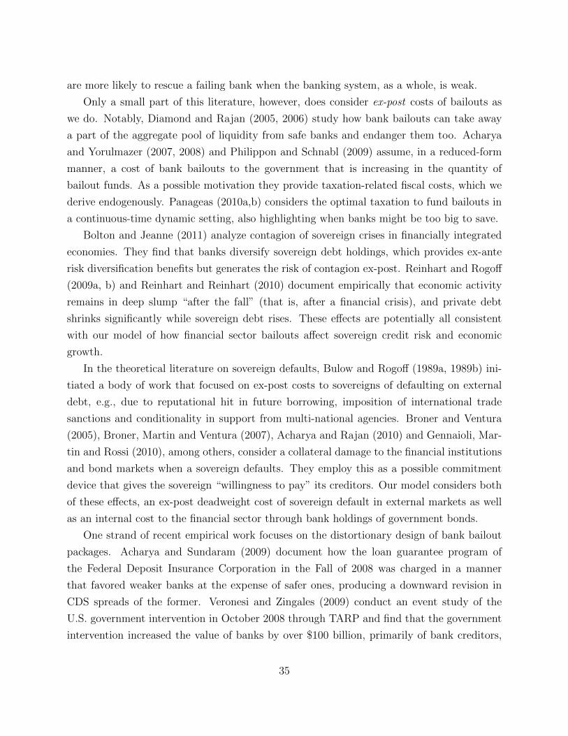
are more likely to rescue a failing bank when the banking system, as a whole, is weak.

Only a small part of this literature, however, does consider ex-post costs of bailouts as

we do. Notably, Diamond and Rajan (2005, 2006) study how bank bailouts can take away

a part of the aggregate pool of liquidity from safe banks and endanger them too. Acharya

and Yorulmazer (2007, 2008) and Philippon and Schnabl (2009) assume, in a reduced-form

manner, a cost of bank bailouts to the government that is increasing in the quantity of

bailout funds. As a possible motivation they provide taxation-related fiscal costs, which we

derive endogenously. Panageas (2010a,b) considers the optimal taxation to fund bailouts in

a continuous-time dynamic setting, also highlighting when banks might be too big to save.

Bolton and Jeanne (2011) analyze contagion of sovereign crises in financially integrated

economies. They find that banks diversify sovereign debt holdings, which provides ex-ante

risk diversification benefits but generates the risk of contagion ex-post. Reinhart and Rogoff

(2009a, b) and Reinhart and Reinhart (2010) document empirically that economic activity

remains in deep slump “after the fall” (that is, after a financial crisis), and private debt

shrinks significantly while sovereign debt rises. These effects are potentially all consistent

with our model of how financial sector bailouts affect sovereign credit risk and economic

growth.

In the theoretical literature on sovereign defaults, Bulow and Rogoff (1989a, 1989b) ini-

tiated a body of work that focused on ex-post costs to sovereigns of defaulting on external

debt, e.g., due to reputational hit in future borrowing, imposition of international trade

sanctions and conditionality in support from multi-national agencies. Broner and Ventura

(2005), Broner, Martin and Ventura (2007), Acharya and Rajan (2010) and Gennaioli, Mar-

tin and Rossi (2010), among others, consider a collateral damage to the financial institutions

and bond markets when a sovereign defaults. They employ this as a possible commitment

device that gives the sovereign “willingness to pay” its creditors. Our model considers both

of these effects, an ex-post deadweight cost of sovereign default in external markets as well

as an internal cost to the financial sector through bank holdings of government bonds.

One strand of recent empirical work focuses on the distortionary design of bank bailout

packages. Acharya and Sundaram (2009) document how the loan guarantee program of

the Federal Deposit Insurance Corporation in the Fall of 2008 was charged in a manner

that favored weaker banks at the expense of safer ones, producing a downward revision in

CDS spreads of the former. Veronesi and Zingales (2009) conduct an event study of the

U.S. government intervention in October 2008 through TARP and find that the government

intervention increased the value of banks by over $100 billion, primarily of bank creditors,

35

but also estimate a tax payer cost between $25 to $47 billion. Kacperczyk and Schnabl (2010)

examine the government bailout of U.S. money market funds after the Lehman bankruptcy

and find that less well-capitalized money market fund sponsors benefited more from the

bailouts. Panetta et al. (2009) and King (2009) assess the Euro zone bailouts and reach

the conclusion that while bank equity was wiped out in most cases, bank creditors were

backstopped reflecting a waiting game on part of bank regulators and governments. Laeven

and Valencia (2010) put together a time-series of banking crises and examine their economic

costs. They too find that the median output loss of recent banking crises was large and

accounted for about 25% of GDP.

Another strand of recent empirical work relating financial sector and sovereign credit

risk during the ongoing crisis shares some similarity to our paper. Sgherri and Zoli (2009),

Attinasi, Checherita and Nickel (2009), Alter and Schueler (2011), Mody and Sandri (2011),

and Ejsing and Lemke (2011) focus on the effect of bank bailouts on sovereign credit risk

measured using CDS spreads. Some of their evidence mirrors our descriptive evidence.

Dieckmann and Plank (2009) analyze sovereign CDS of developed economies around the

crisis and document a significant rise in co-movement following the collapse of Lehman

Brothers. Demirguc-Kunt and Huizinga (2010) do an international study of equity prices

and CDS spreads around bank bailouts and show that some large banks may be too big to

save rather than too big to fail. Our analysis corroborates and complements some of this

work. In particular, our empirical investigation of banking sector holdings of government

debt, identifying the effect of government guarantees, and how to introduce a linkage between

bank CDS and sovereign CDS is novel.

6 Conclusion

In this paper, we examine the intimate and intricate link between bank bailouts and sovereign

credit risk. In our model, the government faces an important trade-off: bank bailouts ame-

liorate the under-investment problem in the financial sector but reduce the investment in-

centives of the non-financial sector due to the corresponding increase in future taxation. In

the short-run, bailouts are funded through the issuance of government bonds. A high level

of issuance helps to fund the bailout but dilutes existing bondholders and introduces credit

risk into the government bond price. This creates a two-way feedback between sovereign and

financial sector credit risk because financial firms are exposed to the value of government

debt through both their direct bond holdings and via the value of explicit government guar-

36

antees or an implicit safety net. Using bank and sovereign credit default swap data from the

financial crisis of 2007 to 2010, we provide strong evidence of such a two-way feedback.

Overall, we consider the emergence of meaningful sovereign credit risk as an important

potential cost of bank bailouts. This cost of bailouts can render the immediate stabilization

of the financial sector a Pyrrhic victory, but it has received little theoretical attention and

has also not been analyzed much empirically. Taking cognizance of this ultimate cost of

bailouts has important consequences for the future resolution of financial crises, the design

of fiscal policy, and the nexus between the two.

References

Acharya, Viral V. and Raghuram G. Rajan, 2010, “Sovereign Debt, Government Myopia,

and the Financial Sector”, Work in progress, New York University Stern School of

Business.

Acharya, Viral, Hyun Song Shin and Tanju Yorulmazer, 2008, “Crisis Resolution and Bank

Liquidity”, Review of Financial Studies, forthcoming.

Acharya, Viral V. and Rangarajan Sundaram, 2009, “The Financial Sector ‘Bailout’: Sow-

ing the Seeds of the Next Crisis”, Chapter 15 in Acharya, Viral V. and Matthew

Richardson (editors), 2009. “Restoring Financial Stability: How to Repair a Failed

System”, New York University Stern School of Business, John Wiley & Sons.

Acharya, Viral V. and Tanju Yorulmazer, 2007 “Too Many to Fail - An Analysis of Time-

inconsistency in Bank Closure Policies,” Journal of Financial Intermediation, 16(1),

1–31.

Acharya, Viral V. and Tanju Yorulmazer, 2008, “Cash-in-the-Market Pricing and Optimal

Resolution of Bank Failures,” Review of Financial Studies, 21, 2705–2742.

Aghion, Philipp, Patrick Bolton and Steven Fries, 1999, “Optimal Design of Bank Bailouts:

The Case of Transition Economies”, Journal of Institutional and Theoretical Eco-

nomics, 155, 51–70.

Alter, Adrian, and Yves Schueler, 2011, “Credit Spread Interdependencies of European

States and Banks during the Financial Crisis”, Working Paper.

37

Attinasi, Maria-Grazia, Cristina Checherita and Christiane Nickel, 2009, “What Explains

the Surge in Euro Area Sovereign Spreads during the Financial Crisis of 2007-09?”,

European Central Bank Working Paper No. 1131.

Bhattacharya, Sudipto and Kjell G. Nyborg, 2010, “Bank Bailout Menus”, Swiss Finance

Institute Research Paper Series No. 10–24.

Bolton, Patrick and Olivier Jeanne, 2011, “Sovereign Default Risk and Bank Fragility in

Financially Integrated Economies,” NBER Working Paper 16899

Broner, Martin and Jaume Ventura, 2005, “Globalization and Risk Sharing”, Working

Paper, Universitat Pompeu Fabra.

Broner, Martin, Alberto Martin and Jaume Ventura, 2007, “Enforcement Problems and

Secondary Markets”, Working Paper, Universitat Pompeu Fabra.

Brown, C. and Dinc, S., 2009, “Too Many to fail? Evidence of regulatory forbearance When

the banking sector is weak”, Review of financial Studies, forthcoming.

Bulow, J., and K. Rogoff, 1989a, “Sovereign debt: Is to forgive to forget?”, American

Economic Review, 79, 43-50.

Bulow, J., and K. Rogoff, 1989b, “A constant recontracting model of sovereign debt”,

Journal of Political Economy, 97, 155-178.

Collin-Dufresne, Pierre, Robert S. Goldstein and J. Spencer Martin, 2001, “The Determi-

nants of Credit Spread Changes”, Journal of Finance, 56(6), 2177-2207.

Demirguc-Kunt, Asli and Harry Huizinga, 2010, “Are Banks Too Big to Fail or Too Big

to Save? International Evidence from Equity Prices and CDS Spreads”, World Bank

Policy Research Working Paper 5360.

Diamond, Douglas and Raghuram G. Rajan, 2005, “Liquidity Shortages and Banking

Crises”, Journal of Finance, 60(2), 615–647.

Diamond, Douglas and Raghuram G. Rajan, 2006, “Bank Bailouts and Aggregate Liquid-

ity”, American Economic Review Papers and Proceedings, 92(2), 38–41.

Diamond, Douglas and Raghuram G. Rajan, 2009, “Fear of Fire Sales, Illiquidity Seeking

and Credit Freeze”, Quarterly Journal of Economics, forthcoming.

38

Dieckmann, Stephan and Thomas Plank, 2009, “Default Risk of Advanced Economies:

An Empirical Analysis of Credit Default Swaps during the Financial Crisis”, Working

Paper, Wharton School of Business, University of Pennsylvania.

Ejsing, Jacob and Wolfgang Lemke, 2011, “The Janus-headed salvation: Sovereign and

bank credit risk premia during 2008-2009,” Economics Letters, 110, 28–31.

Gennaioli, Nicola, Alberto Martin and Stefano Rossi, 2010, “Sovereign Default, Domestic

Banks and Financial Institutions”, Working Paper, Universitat Pompeu Fabra.

Gorton, Gary and Lixin Huang. 2004. “Liquidity, Efficiency, and Bank Bailouts” American

Economic Review, 94(3): 455-483.

Kacperczyk, Marcin and Philipp Schnabl, 2010, “Implicit Guarantees and Risk-taking:

Evidence from Money Market Funds”, New York University Stern School of Business.

King, Michael R, 2009, “Time to Buy or Just Buying Time? The Market Reaction to Bank

Rescue Packages”, BIS Papers No 288 (September).

Laeven, Luc and Fabian Valencia, 2010, “Resolution of Banking Crises: The Good, the

Bad, and the Ugly,” IMF Working Paper

Mailath, George and Loretta Mester, 1994, “A Positive Analysis of Bank Closure”, Journal

of Financial Intermediation, 3(3), 272–299.

Merton, Robert C., 1974, “On the Pricing of Corporate Debt: The Risk Structure of Interest

Rates”, Journal of Finance, 29, 449-470.

Mody, Ashoka, and Sandri, Damiano, “From Bear Stearns through Anglo Irish: How a

Financial Crisis Turned into a Sovereign Crisis”, IMF Working Paper.

Moody’s Investors Services, 8 October 2008, ”Moody’s downgrades Iceland’s ratings to A1

from Aa1”.

Myers, Stewart C., 1977, “The Determinants of Corporate Borrowing”, Journal of Financial

Economics, 5(2), 147–175.

Panageas, Stavros, 2010a, “Optimal taxation in the presence of bailouts”, Journal of Mon-

etary Economics, 57, 101?-116.

39

Panageas, Stavros, 2010b, “Bailouts,the incentive to manage risk,and financial crises”, Jour-

nal of Financial Economics, 95, 296?-311.

Panetta, Faib, Thomas Faeh, Giuseppe Grande, Corrinne Ho, Michael King, Aviram Levy,

Federico M Signoretti, Marco Taboga, and Andrea Zaghini, 2009, “An Assessment of

Financial Sector Rescue Programmes”, BIS Papers No 48 (July).

Penati, A. and Protopapadakis, A., 1988, “The effect of implicit deposit insurance on

banks? portfolio choices, with an application to international overexposure”, Journal

of Monetary Economics, 21(1), 107–126.

Philippon, Thomas and Philipp Schnabl, 2009, “Efficient Recapitalization”, Working Paper,

New York University Stern School of Business.

Reinhart, Carmen M. and Vincent Reinhart, 2010, “After the Fall”, presentation at the

Federal Reserve Bank of Kansas City Economic Symposium at Jackson Hole, Wyoming,

August 27, 2010.

Reinhart, Carmen M. and Kenneth S. Rogoff, 2009a, This Time Is Different: Eight Cen-

turies of Financial Folly, Princeton University Press.

Reinhart, Carmen M. and Kenneth S. Rogoff, 2009b, “Growth in a Time of Debt”, American

Economic Review Papers and Proceedings, forthcoming.

Sgherri, Silvia and Edda Zoli, 2009, “Euro Area Sovereign Risk During the Crisis”, Working

paper, International Monetary Fund, No. 09–222.

Veronesi, P. and Zingales, L., 2009, “Paulson’s Gift”, Journal of Financial Economics,

forthcoming.

40

Fig

ure

1:Sov

erei

gnC

DS

and

Ban

kC

DS

ofIr

elan

d

0

100

200

300

400

500

600

700

basis points

Sovereign CD

S

Avg. Bank CD

S

Fig

ure

1p

lots

the

sove

reig

nC

DS

and

ban

kC

DS

for

Irel

and

inth

ep

erio

dfr

om3/

1/20

07to

8/31/2010.

Th

eb

an

kC

DS

isco

mp

ute

das

the

unw

eigh

ted

aver

age

ofb

ank

CD

Sfo

rb

anks

hea

dqu

arte

red

inIr

elan

d(A

llie

dIr

ish

Ban

k,

An

glo

Iris

hB

ank,

Ban

kof

Irel

and

,an

dIr

ish

Lif

ean

dP

erm

anen

t).

Th

ed

ata

are

from

Dat

astr

eam

.

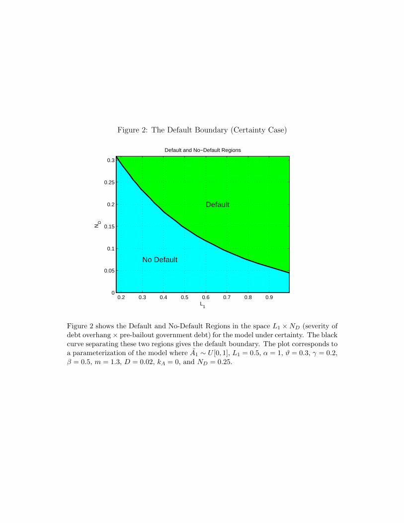
Figure 2: The Default Boundary (Certainty Case)

Default and No−Default Regions

L1

ND

Default

No Default

0.2 0.3 0.4 0.5 0.6 0.7 0.8 0.90

0.05

0.1

0.15

0.2

0.25

0.3

Figure 2 shows the Default and No-Default Regions in the space L1 ×ND (severity ofdebt overhang× pre-bailout government debt) for the model under certainty. The blackcurve separating these two regions gives the default boundary. The plot corresponds toa parameterization of the model where A1 ∼ U [0, 1], L1 = 0.5, α = 1, ϑ = 0.3, γ = 0.2,β = 0.5, m = 1.3, D = 0.02, kA = 0, and ND = 0.25.

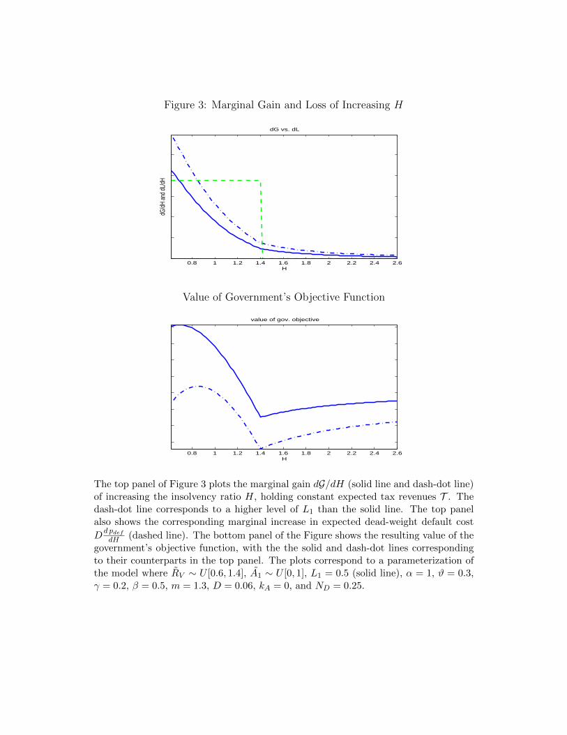
Figure 3: Marginal Gain and Loss of Increasing H

0.8 1 1.2 1.4 1.6 1.8 2 2.2 2.4 2.6H

dG/d

H an

d dL

/dH

dG vs. dL

Value of Government’s Objective Function

0.8 1 1.2 1.4 1.6 1.8 2 2.2 2.4 2.6H

value of gov. objective

The top panel of Figure 3 plots the marginal gain dG/dH (solid line and dash-dot line)of increasing the insolvency ratio H, holding constant expected tax revenues T . Thedash-dot line corresponds to a higher level of L1 than the solid line. The top panelalso shows the corresponding marginal increase in expected dead-weight default cost

Dd pdefdH (dashed line). The bottom panel of the Figure shows the resulting value of the

government’s objective function, with the the solid and dash-dot lines correspondingto their counterparts in the top panel. The plots correspond to a parameterization ofthe model where RV ∼ U [0.6, 1.4], A1 ∼ U [0, 1], L1 = 0.5 (solid line), α = 1, ϑ = 0.3,γ = 0.2, β = 0.5, m = 1.3, D = 0.06, kA = 0, and ND = 0.25.

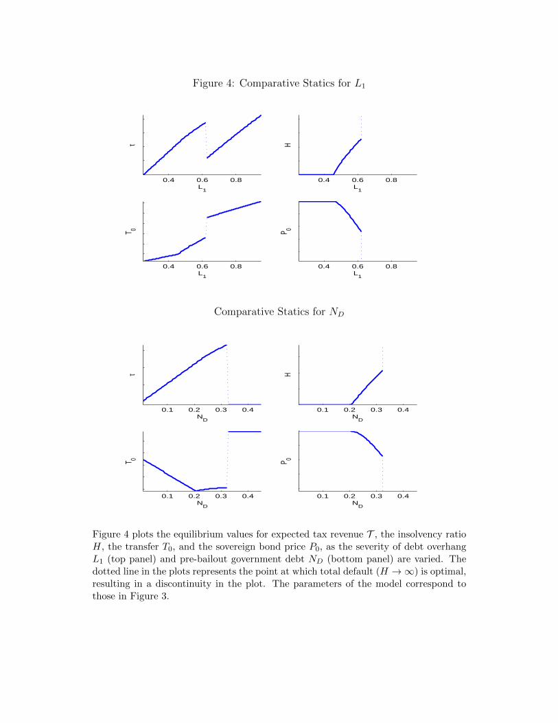
Figure 4: Comparative Statics for L1

0.4 0.6 0.8L

1

τ

0.4 0.6 0.8L

1

H

0.4 0.6 0.8L

1

T 0

0.4 0.6 0.8L

1

P 0

Comparative Statics for ND

0.1 0.2 0.3 0.4N

D

τ

0.1 0.2 0.3 0.4N

D

H

0.1 0.2 0.3 0.4N

D

T 0

0.1 0.2 0.3 0.4N

D

P 0

Figure 4 plots the equilibrium values for expected tax revenue T , the insolvency ratioH, the transfer T0, and the sovereign bond price P0, as the severity of debt overhangL1 (top panel) and pre-bailout government debt ND (bottom panel) are varied. Thedotted line in the plots represents the point at which total default (H →∞) is optimal,resulting in a discontinuity in the plot. The parameters of the model correspond tothose in Figure 3.

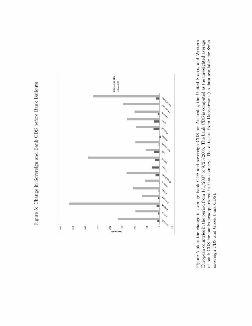
Fig

ure

5:C

han

gein

Sov

erei

gnan

dB

ank

CD

Sb

efor

eB

ank

Bai

louts

‐50050100

150

200

250

300

350

400

basi points

Sovereign CD

S

Bank CDS

Fig

ure

5p

lots

the

chan

gein

aver

age

ban

kC

DS

and

sove

reig

nC

DS

for

Au

stra

lia,

the

Un

ited

Sta

tes,

an

dW

este

rnE

uro

pea

nco

untr

ies

inth

ep

erio

dfr

om1/

1/20

07to

9/25

/200

8.T

he

ban

kC

DS

isco

mp

ute

das

the

unw

eighte

dav

erage

ofb

ank

CD

Sfo

rb

anks

hea

dqu

arte

red

inth

atco

untr

y.T

he

dat

aar

efr

omD

atas

trea

m(n

od

ata

avail

ab

lefo

rS

wis

sso

vere

ign

CD

San

dG

reek

ban

kC

DS

).

Fig

ure

6:C

han

gein

Sov

erei

gnan

dB

ank

CD

Sduri

ng

the

Per

iod

ofB

ank

Bai

louts

‐250

‐200

‐150

‐100‐50050100

basis points

Sovereign CD

S

Bank CDS

Fig

ure

6p

lots

the

chan

gein

aver

age

ban

kC

DS

and

sove

reig

nC

DS

for

Au

stra

lia,

the

Un

ited

Sta

tes,

an

dW

este

rnE

uro

pea

nco

untr

ies

inth

ep

erio

dfr

om9/

26/2

008

to10

/21/

2008

.T

he

ban

kC

DS

isco

mp

ute

das

the

unw

eighte

dav

erag

eof

ban

kC

DS

for

ban

ks

hea

dqu

arte

red

inth

atco

untr

y.T

he

dat

aar

efr

omD

atas

trea

m(n

od

ata

avail

ab

lefo

rS

wis

sso

vere

ign

CD

San

dG

reek

ban

kC

DS

).

Fig

ure

7:C

han

gein

Sov

erei

gnan

dB

ank

CD

Saf

ter

Ban

kB

ailo

uts

‐2000

200

400

600

800

1,000

1,200

basis points

Sovereign CD

S

Bank CDS

Fig

ure

7p

lots

the

chan

gein

aver

age

ban

kC

DS

and

sove

reig

nC

DS

for

Au

stra

lia,

the

Un

ited

Sta

tes,

an

dW

este

rnE

uro

pea

nco

untr

ies

inth

ep

erio

dfr

om10

/22/

2008

to6/

30/2

010.

Th

eb

ank

CD

Sis

com

pu

ted

as

the

unw

eighte

dav

erag

eof

ban

kC

DS

for

ban

ks

hea

dqu

arte

red

inth

atco

untr

y.T

he

dat

aar

efr

omD

atas

trea

m.

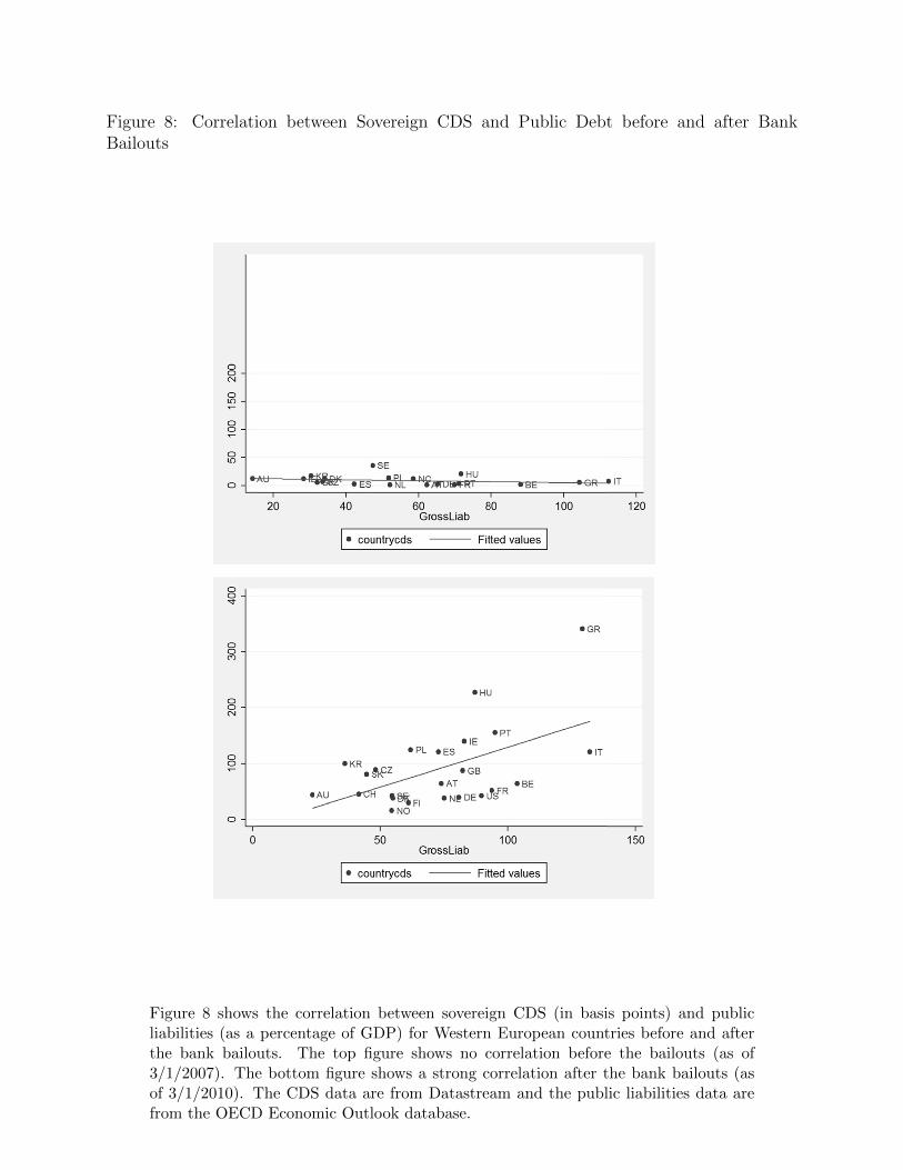
Figure 8: Correlation between Sovereign CDS and Public Debt before and after BankBailouts

Figure 8 shows the correlation between sovereign CDS (in basis points) and publicliabilities (as a percentage of GDP) for Western European countries before and afterthe bank bailouts. The top figure shows no correlation before the bailouts (as of3/1/2007). The bottom figure shows a strong correlation after the bank bailouts (asof 3/1/2010). The CDS data are from Datastream and the public liabilities data arefrom the OECD Economic Outlook database.

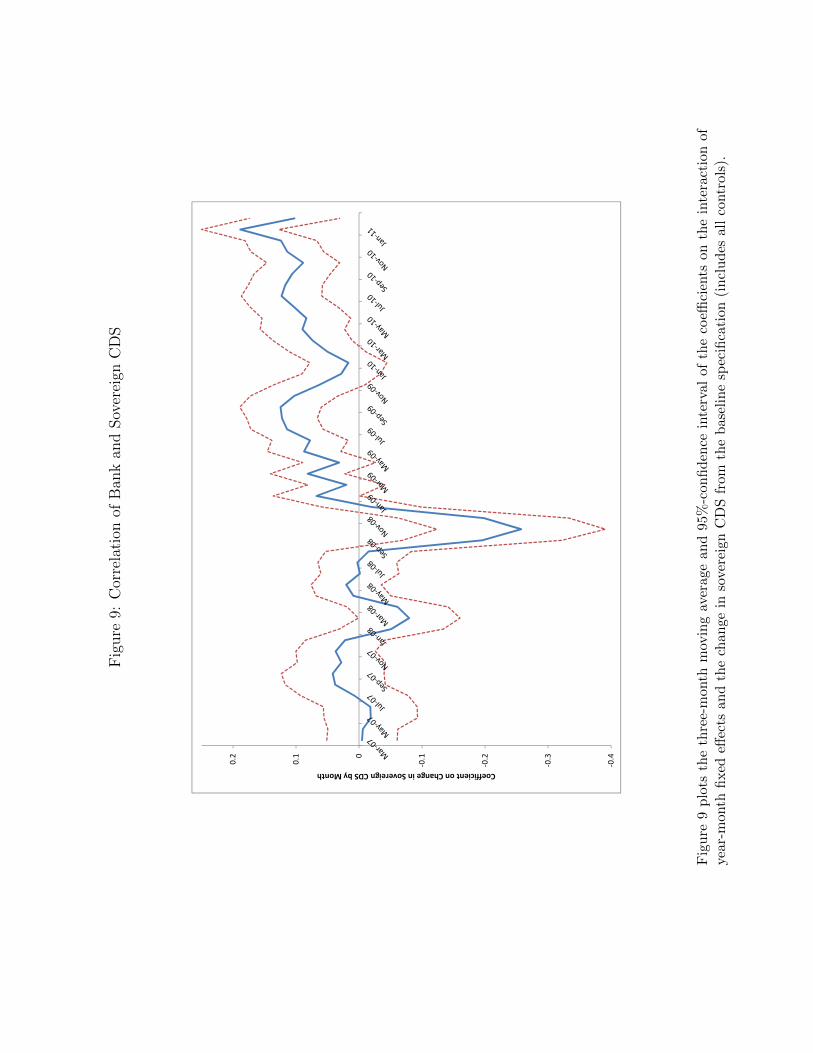
Fig

ure

9:C

orre

lati

onof

Ban

kan

dSov

erei

gnC

DS

‐0.4

‐0.3

‐0.2

‐0.10

0.1

0.2

Coefficient on Change in Sovereign CDS by Month

Fig

ure

9p

lots

the

thre

e-m

onth

mov

ing

aver

age

and

95%

-con

fid

ence

inte

rval

ofth

eco

effici

ents

on

the

inte

ract

ion

of

year

-mon

thfi

xed

effec

tsan

dth

ech

ange

inso

vere

ign

CD

Sfr

omth

eb

asel

ine

spec

ifica

tion

(in

clu

des

all

contr

ols

).

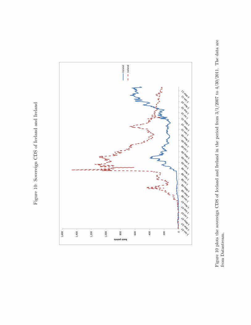
Fig

ure

10:

Sov

erei

gnC

DS

ofIc

elan

dan

dIr

elan

d

0

200

400

600

800

1,00

0

1,20

0

1,40

0

1,60

0

basis points

Ireland

Iceland

Fig

ure

10p

lots

the

sove

reig

nC

DS

ofIc

elan

dan

dIr

elan

din

the

per

iod

from

3/1/

2007

to4/

30/2011.

Th

ed

ata

are

from

Dat

astr

eam

.

Table 1: Summary Statistics

The sample shows summary statistics on bank and sovereign credit risk. The sample includes all European, U.S., and Australian banks with available data on bank CDS, sovereign CDS, and equity returns. The data are at the weekly level. Panel A presents summary statistics for the first week of July 2007. Panel B presents summary statistics for the period before, around, and after the bailouts.

Panel A: Cross-Section (7/1/2007)

   # Mean Std.Dev 50th percentile 5th percentile 95th percentile

Assets ($ billion) 81 589.3 594.9 362.6 77.9 1,896.90Equity ($ billion) 81 26.8 29.3 20.2 3.5 112.4Equity Ratio (%) 81 5.1 2.7 4.8 1.9 10Tier 1 Ratio (%) 66 8.5 1.9 8.2 6.5 12.4Bank CDS (bp) 75 21.8 13.4 10.5 6.5 41

Sovereign CDS (bp) 56 6.6 11.5 2 1.5 52.1

Panel B: Time-Series

Pre-Bailout (1/1/2007-9/17/2008)

   # Mean Std.Dev 50th percentile 5th percentile 95th percentile

Bank CDS (bp) 2,891 93.2 129 67.7 6.6 271.2Sovereign CDS (bp) 2,891 13.5 12.1 9.6 1.8 38.3∆ Bank CDS (%) 2,891 0.038 0.247 0.025 -0.242 0.329∆ Sovereign CDS (%) 2,891 0.024 0.3 0.028 -0.256 0.318Bank Stock Return (%) 2,891 -0.011 0.084 -0.006 -0.116 0.081∆ CDS Market Index (%) 2,891 0.021 0.118 0.005 -0.141 0.211∆ Volatility (%) 2,891 0.003 0.032 0.002 -0.038 0.043

Bailout (9/18/2008-10/22/2008)

Bank CDS (bp) 254 288.6 626.0 133.3 70.0 740.0Sovereign CDS (bp) 254 39.3 18.8 32.5 12.5 73.5∆ Bank CDS (%) 254 -0.065 0.44 -0.037 -0.629 0.405∆ Sovereign CDS (%) 254 0.146 0.19 0.129 -0.105 0.502Bank Stock Return (%) 254 -0.067 0.268 -0.03 -0.374 0.201∆ CDS Market Index (%) 254 0.017 0.095 0.04 -0.157 0.116∆ Volatility (%) 254 0.048 0.071 0.076 -0.036 0.127

Post-Bailout (10/23/2008 - 30/4/2011)

Bank CDS (bp) 6,500 188.7 179.9 131.2 65.5 560.6Sovereign CDS (bp) 6,500 108.5 142.9 60.1 24.9 347∆ Bank CDS (%) 6,500 0.003 0.12 -0.001 -0.158 0.184∆ Sovereign CDS (%) 6,500 0.004 0.113 0.003 -0.181 0.186Bank Stock Return (%) 6,500 0 0.098 0.002 -0.132 0.129∆ CDS Market Index (%) 6,500 -0.002 0.071 -0.006 -0.113 0.117

∆ Volatility (%) 6,500 -0.003 0.048 -0.004 -0.059 0.06

Table 2: Emergence of Sovereign Credit Risk

This table shows the relation between sovereign credit risk, public debt-to-gdp, and financial sector distress. The sample includes Australia, Denmark, Great Britain, Norway, Sweden, Switzerland, and all Eurozone countries with publicly available data on sovereign CDS and bank CDS. The data are at the country-level. The independent variable in Columns (1) and (2) is the sovereign CDS before the bank bailouts (as of 1/1/2008). Columns (1) and (2) control for Pre-bailout Debt (debt-to-gdp ratio) measured as Government Liabilities as share of GDP (collected from the OECD Economic Outlook). Column (2) controls for financial sector distress measured as the natural logarithm of the average banks CDS before the bank bailouts (as of 9/22/2008). The independent variable in Columns (3) and (4) is the sovereign CDS after the bank bailouts (as of 3/31/2010). The dependent variables are the same as in Columns (1) and (2), respectively. The independent variable in Column (5) is the change in the debt-to-gdp ratio from June 2008 to June 2010. The dependent variable is financial sector distress. The independent variable in column (6) is the debt-to-gdp ratio in June 2010. The dependent variables are the pre-bailout debt-to-GDP ratio and financial sector distress. We report robust standard errors. ** 1% significant, * 5% significant, and + 10% significant

Log (Sovereign CDS) Debt-to-GDP Pre-Bailout Post-Bailout Post-Bailout

1/1/2008 3/31/2010 ∆ 2008-2010 3/31/2010 (1) (2) (3) (4) (5) (6)

Pre-Bailout Debt-to-GDP 0.006 0.005 0.015* 0.013+ 1.107**

(0.004) (0.005) (0.006) (0.007) (0.144) Pre-Bailout Financial Sector Distress 0.311 0.965* 20.118+ 21.726+

(0.208) (0.357) (10.168) (11.555) Constant 2.137** 0.601 3.112** -1.593 -86.920 -101.548

(0.320) (1.154) (0.401) (2.019) (49.456) (60.923)

Observations 15 14 17 15 15 15

R-squared 0.134 0.171 0.261 0.488 0.364 0.843

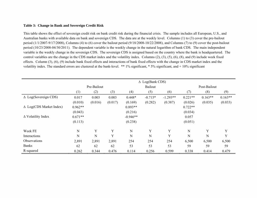
Table 3: Change in Bank and Sovereign Credit Risk

This table shows the effect of sovereign credit risk on bank credit risk during the financial crisis. The sample includes all European, U.S., and Australian banks with available data on bank and sovereign CDS. The data are at the weekly level. Columns (1) to (3) cover the pre-bailout period (1/1/2007-9/17/2008), Columns (4) to (6) cover the bailout period (9/18/2008-10/22/2008), and Columns (7) to (9) cover the post-bailout period (10/23/2008-04/30/2011). The dependent variable is the weekly change in the natural logarithm of bank CDS. The main independent variable is the weekly change in the sovereign CDS. The sovereign CDS is assigned based on the country where the bank is headquartered. The control variables are the change in the CDS market index and the volatility index. Columns (2), (3), (5), (6), (8), and (9) include week fixed effects. Column (3), (6), (9) include bank fixed effects and interactions of bank fixed effects with the change in CDS market index and the volatility index. The standard errors are clustered at the bank-level. ** 1% significant, * 5% significant, and + 10% significant

∆ Log(Bank CDS)

Pre-Bailout Bailout Post-Bailout

(1) (2) (3) (4) (5) (6) (7) (8) (9)

∆ Log(Sovereign CDS) 0.017 0.003 0.003 0.448* -0.715* -1.293** 0.221** 0.163** 0.163** (0.010) (0.016) (0.017) (0.169) (0.282) (0.387) (0.026) (0.035) (0.033)

∆ Log(CDS Market Index) 0.962** 0.893** 0.722** (0.043) (0.216) (0.034)

∆ Volatility Index 0.671** -0.946** 0.057 (0.113) (0.238) (0.051)

Week FE N Y Y N Y Y N Y Y Interactions N N Y N N Y N N Y Observations 2,891 2,891 2,891 254 254 254 6,500 6,500 6,500 Banks 62 62 62 53 53 53 59 59 59 R-squared 0.262 0.344 0.476 0.114 0.256 0.599 0.338 0.414 0.479

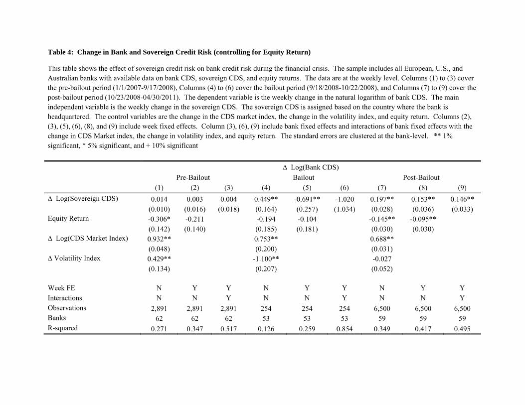
Table 4: Change in Bank and Sovereign Credit Risk (controlling for Equity Return)

This table shows the effect of sovereign credit risk on bank credit risk during the financial crisis. The sample includes all European, U.S., and Australian banks with available data on bank CDS, sovereign CDS, and equity returns. The data are at the weekly level. Columns (1) to (3) cover the pre-bailout period (1/1/2007-9/17/2008), Columns (4) to (6) cover the bailout period (9/18/2008-10/22/2008), and Columns (7) to (9) cover the post-bailout period (10/23/2008-04/30/2011). The dependent variable is the weekly change in the natural logarithm of bank CDS. The main independent variable is the weekly change in the sovereign CDS. The sovereign CDS is assigned based on the country where the bank is headquartered. The control variables are the change in the CDS market index, the change in the volatility index, and equity return. Columns (2), (3), (5), (6), (8), and (9) include week fixed effects. Column (3), (6), (9) include bank fixed effects and interactions of bank fixed effects with the change in CDS Market index, the change in volatility index, and equity return. The standard errors are clustered at the bank-level. ** 1% significant, * 5% significant, and + 10% significant

∆ Log(Bank CDS)

Pre-Bailout Bailout Post-Bailout

(1) (2) (3) (4) (5) (6) (7) (8) (9)

∆ Log(Sovereign CDS) 0.014 0.003 0.004 0.449** -0.691** -1.020 0.197** 0.153** 0.146** (0.010) (0.016) (0.018) (0.164) (0.257) (1.034) (0.028) (0.036) (0.033)

Equity Return -0.306* -0.211 -0.194 -0.104 -0.145** -0.095** (0.142) (0.140) (0.185) (0.181) (0.030) (0.030)

∆ Log(CDS Market Index) 0.932** 0.753** 0.688** (0.048) (0.200) (0.031)

∆ Volatility Index 0.429** -1.100** -0.027 (0.134) (0.207) (0.052)

Week FE N Y Y N Y Y N Y Y Interactions N N Y N N Y N N Y Observations 2,891 2,891 2,891 254 254 254 6,500 6,500 6,500 Banks 62 62 62 53 53 53 59 59 59 R-squared 0.271 0.347 0.517 0.126 0.259 0.854 0.349 0.417 0.495

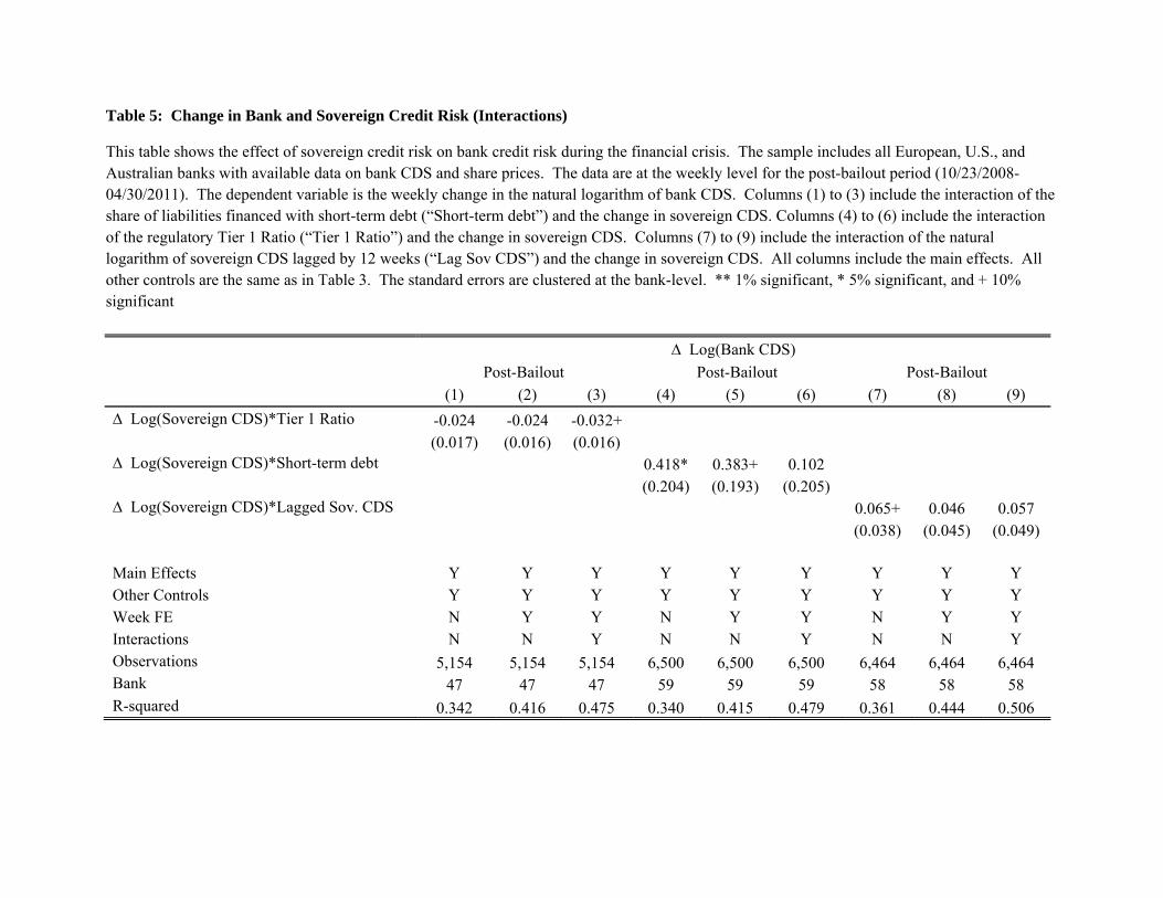
Table 5: Change in Bank and Sovereign Credit Risk (Interactions)

This table shows the effect of sovereign credit risk on bank credit risk during the financial crisis. The sample includes all European, U.S., and Australian banks with available data on bank CDS and share prices. The data are at the weekly level for the post-bailout period (10/23/2008-04/30/2011). The dependent variable is the weekly change in the natural logarithm of bank CDS. Columns (1) to (3) include the interaction of the share of liabilities financed with short-term debt (“Short-term debt”) and the change in sovereign CDS. Columns (4) to (6) include the interaction of the regulatory Tier 1 Ratio (“Tier 1 Ratio”) and the change in sovereign CDS. Columns (7) to (9) include the interaction of the natural logarithm of sovereign CDS lagged by 12 weeks (“Lag Sov CDS”) and the change in sovereign CDS. All columns include the main effects. All other controls are the same as in Table 3. The standard errors are clustered at the bank-level. ** 1% significant, * 5% significant, and + 10% significant

∆ Log(Bank CDS)

Post-Bailout Post-Bailout Post-Bailout

(1) (2) (3) (4) (5) (6) (7) (8) (9)

∆ Log(Sovereign CDS)*Tier 1 Ratio -0.024 -0.024 -0.032+ (0.017) (0.016) (0.016)

∆ Log(Sovereign CDS)*Short-term debt 0.418* 0.383+ 0.102 (0.204) (0.193) (0.205) ∆ Log(Sovereign CDS)*Lagged Sov. CDS 0.065+ 0.046 0.057

(0.038) (0.045) (0.049)

Main Effects Y Y Y Y Y Y Y Y Y Other Controls Y Y Y Y Y Y Y Y Y Week FE N Y Y N Y Y N Y Y Interactions N N Y N N Y N N Y Observations 5,154 5,154 5,154 6,500 6,500 6,500 6,464 6,464 6,464 Bank 47 47 47 59 59 59 58 58 58 R-squared 0.342 0.416 0.475 0.340 0.415 0.479 0.361 0.444 0.506

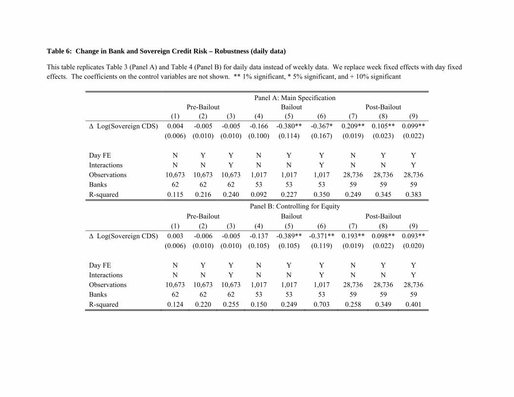
Table 6: Change in Bank and Sovereign Credit Risk – Robustness (daily data)

This table replicates Table 3 (Panel A) and Table 4 (Panel B) for daily data instead of weekly data. We replace week fixed effects with day fixed effects. The coefficients on the control variables are not shown. ** 1% significant, * 5% significant, and + 10% significant

Panel A: Main Specification Pre-Bailout Bailout Post-Bailout

(1) (2) (3) (4) (5) (6) (7) (8) (9)

∆ Log(Sovereign CDS) 0.004 -0.005 -0.005 -0.166 -0.380** -0.367* 0.209** 0.105** 0.099**(0.006) (0.010) (0.010) (0.100) (0.114) (0.167) (0.019) (0.023) (0.022)

Day FE N Y Y N Y Y N Y Y Interactions N N Y N N Y N N Y Observations 10,673 10,673 10,673 1,017 1,017 1,017 28,736 28,736 28,736 Banks 62 62 62 53 53 53 59 59 59

R-squared 0.115 0.216 0.240 0.092 0.227 0.350 0.249 0.345 0.383

Panel B: Controlling for Equity

Pre-Bailout Bailout Post-Bailout (1) (2) (3) (4) (5) (6) (7) (8) (9)

∆ Log(Sovereign CDS) 0.003 -0.006 -0.005 -0.137 -0.389** -0.371** 0.193** 0.098** 0.093**(0.006) (0.010) (0.010) (0.105) (0.105) (0.119) (0.019) (0.022) (0.020)

Day FE N Y Y N Y Y N Y Y Interactions N N Y N N Y N N Y Observations 10,673 10,673 10,673 1,017 1,017 1,017 28,736 28,736 28,736 Banks 62 62 62 53 53 53 59 59 59

R-squared 0.124 0.220 0.255 0.150 0.249 0.703 0.258 0.349 0.401

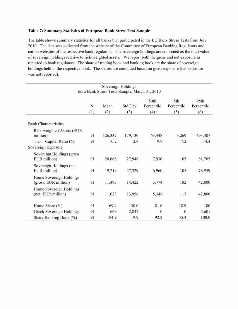
Table 7: Summary Statistics of European Bank Stress Test Sample

The table shows summary statistics for all banks that participated in the EU Bank Stress Tests from July 2010. The data was collected from the website of the Committee of European Banking Regulators and nation websites of the respective bank regulators. The sovereign holdings are computed as the total value of sovereign holdings relative to risk-weighted assets. We report both the gross and net exposure as reported to bank regulators. The share of trading book and banking book are the share of sovereign holdings held in the respective book. The shares are computed based on gross exposure (net exposure was not reported).

Sovereign Holdings Euro Bank Stress Tests Sample, March 31, 2010

N Mean Std.Dev 50th

Percentile 5th

Percentile 95th

Percentile (1) (2) (3) (4) (5) (6)

Bank Characteristics

Risk-weighted Assets (EUR million) 91 126,337 179,130 63,448 3,269 493,307

Tier 1 Capital Ratio (%) 91 10.2 2.4 9.8 7.2 14.4Sovereign Exposure

Sovereign Holdings (gross, EUR million) 91 20,668 27,948 7,930 105 81,765

Sovereign Holdings (net, EUR million) 91 19,719 27,329 6,960 105 78,959

Home Sovereign Holdings (gross, EUR million) 91 11,493 14,422 5,774 182 42,800

Home Sovereign Holdings (net, EUR million) 91 11,023 13,956 5,348 117 42,800

Home Share (%) 91 69.4 30.0 81.6 18.9 100 Greek Sovereign Holdings 91 669 2,844 0 0 5,601 Share Banking Book (%) 91 84.9 19.9 92.2 35.4 100.0

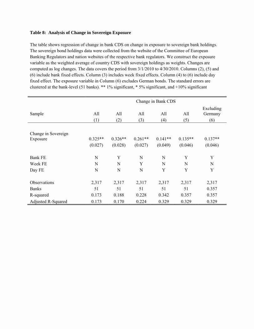
Table 8: Analysis of Change in Sovereign Exposure The table shows regression of change in bank CDS on change in exposure to sovereign bank holdings. The sovereign bond holdings data were collected from the website of the Committee of European Banking Regulators and nation websites of the respective bank regulators. We construct the exposure variable as the weighted average of country CDS with sovereign holdings as weights. Changes are computed as log changes. The data covers the period from 3/1/2010 to 4/30/2010. Columns (2), (5) and (6) include bank fixed effects. Column (3) includes week fixed effects. Column (4) to (6) include day fixed effect. The exposure variable in Column (6) excludes German bonds. The standard errors are clustered at the bank-level (51 banks). ** 1% significant, * 5% significant, and +10% significant

Change in Bank CDS

Sample All All All All All Excluding Germany

(1) (2) (3) (4) (5) (6)

Change in Sovereign Exposure 0.325** 0.326** 0.261** 0.141** 0.135** 0.137**

(0.027) (0.028) (0.027) (0.049) (0.046) (0.046)

Bank FE N Y N N Y Y Week FE N N Y N N N Day FE N N N Y Y Y

Observations 2,317 2,317 2,317 2,317 2,317 2,317 Banks 51 51 51 51 51 0.357 R-squared 0.173 0.188 0.228 0.342 0.357 0.357

Adjusted R-Squared 0.173 0.170 0.224 0.329 0.329 0.329