1

A Quantile Regression Analysis of the Cross Sectionof Stock Market Returns

Michelle L. Barnesa1 and Anthony W. Hughesb

aFederal Reserve Bank of Boston,

T-8, Research

600 Atlantic Avenue,

Boston, MA 02106

USAbSchool of Economics,

University of Adelaide

Adelaide, SA 5005

Australia

Current Draft: November 2002.

Key Words: Capital Asset Pricing Model (CAPM); semi-parametric regression;

errors-in-variables; Monte Carlo simulation; cross-section analysis; underper-

forming stocks and overperforming stocks.

JEL Classifications: G12; C14; C21.

Abstract

Traditional methods of modelling returns and testing the Capital Asset Pricing Model

(CAPM) do so at the mean of the conditional distribution. Instead, we model returns and

test whether the conditional CAPM holds at other points of the distribution by utilizing

the technique of quantile regression (Koenker and Bassett 1978). This method allows us

to model the performance of firms or portfolios that underperform or overperform in the

sense that the conditional mean under- or overpredicts the firm’s return. In the context

of a conditional CAPM, the market price of beta risk is significant in both tails of the

conditional distribution of returns - negative for firms that underperform and positive for

firms that overperform - but is insignificant around the median, and the opposite pattern

obtains for large firms. Underperforming firms exhibit a positive relationship between size

and returns in support of Merton’s (1987) prediction, and there is some evidence of a

positive relationship between returns and financial paper for overperforming firms. Quantile

regression alleviates some of the statistical problems which plague CAPM studies: errors-in-

variables; omitted variables bias; sensitivity to outliers; and non-normal error distributions.

1Corresponding author, e-mail michelle.barnes@bos.frb.org. The views expressed in this paper do notnecessarily reflect those of the Federal Reserve System.

2

A Quantile Regression Analysis of the Cross Sectionof Stock Market Returns

Current Draft: November 2002.

Key Words: Capital Asset Pricing Model (CAPM); semi-parametric regression;

errors-in-variables; Monte Carlo simulation; cross-section analysis; underper-

forming stocks and overperforming stocks.

JEL Classifications: G12; C14; C21.

Abstract

Traditional methods of modelling returns and testing the Capital Asset Pricing Model

(CAPM) do so at the mean of the conditional distribution. Instead, we model returns and

test whether the conditional CAPM holds at other points of the distribution by utilizing

the technique of quantile regression (Koenker and Bassett 1978). This method allows us

to model the performance of firms or portfolios that underperform or overperform in the

sense that the conditional mean under- or overpredicts the firm’s return. In the context

of a conditional CAPM, the market price of beta risk is significant in both tails of the

conditional distribution of returns - negative for firms that underperform and positive for

firms that overperform - but is insignificant around the median, and the opposite pattern

obtains for large firms. Underperforming firms exhibit a positive relationship between size

and returns in support of Merton’s (1987) prediction, and there is some evidence of a

positive relationship between returns and financial paper for overperforming firms. Quantile

regression alleviates some of the statistical problems which plague CAPM studies: errors-in-

variables; omitted variables bias; sensitivity to outliers; and non-normal error distributions.

3

1. Introduction

Classic approaches to modelling returns and testing the Capital Asset Pricing Model

(CAPM) of Sharpe (1964), Lintner (1965), Mossin (1966) and Black (1972) include the two-

pass method of Fama and MacBeth (1973), the generalized method of moments (GMM)

approach of Harvey (1989), and MacKinlay and Richardson (1991) and the seemingly un-

related regression (SUR) approach of Gibbons (1982) and Gibbons, Ross, and Shanken

(1989). All of these methods and their embellishments effectively model returns and test

the CAPM at the mean of the conditional distribution of returns; that is, they model and

test assets that behave as the mean would predict that they behave.

It is in the second, cross-sectional pass of the Fama and MacBeth (1973) framework that

most researchers have tried to improve upon the traditional method. The innovation of the

present paper is to use the quantile estimator developed by Koenker and Bassett (1978), and

popularized, in part, by Buchinsky (1998), in the second stage of the Fama and MacBeth

(FM) regressions. By so doing, it is possible to model the relationship between returns

and beta not just for those firms that behave according to the mean of the conditional

distribution, but also for firms that overperform and underperform relative to the mean.

In this sense, not only are we evaluating the CAPM relationship at different points in

the conditional distribution, we are also exploring why conditional mean approaches have

yielded ambiguous results regarding the impact of beta on returns.2 Quantile regression

methodology provides a way of understanding and testing how the relationship between

returns and other conditioning variables or risk factors changes across the distribution of

conditional returns, it is these changes that are our primary focus here. We demonstrate

that the marginal effects differ greatly, both across firm size and conditional quantile. In so

doing, we add new evidence to the debates on the relationships between beta and returns,

size and returns, and financial paper and returns.

A fortunate by-product of using this approach is that we can address some of the statisti-

cal problems that have plagued the literature. The standard problem faced by the two-pass

method is errors-in-variables (EIV).3 Starting with Fama and MacBeth (1973), studies in

the two-pass tradition try to solve the EIV problem by grouping the firms into portfolios4

2If the coefficient on beta is of opposite sign at opposite ends of the distribution of conditional returns,then at some point in the distribution the coefficient will pass through zero. In fact, we show that thisis the case in the empirical example considered here, and that the zero point is around the center of thedistribution of conditional returns, underscoring the fact that looking at just the conditional mean cansweep a lot of interesting economic relationships under the carpet. In this case, it can lead us to conclude,as much of the literature has concluded, that beta is insignificant, whereas it is statistically significant forunder- and over-performing firms.

3This approach performs time-series estimation of beta in the first step, and then uses these estimatesin the second stage cross-sectional regression of returns on the time-series estimates of beta along with anyother variables thought to be correlated with the cross section of returns.

4The rationale for this procedure is that if the errors in the betas for the different firms are not perfectly

4

per Blume’s (1970) suggestion.5 Shanken (1992) derives an asymptotically valid correction

to the precision of the Fama and MacBeth (FM) estimates of the price of beta risk due to the

EIV problem.6 Both the approaches of Gibbons (1982) and Harvey (1989) were developed

in large part to ameliorate the EIV problem by simultaneously exploiting the time-series

and cross-sectional dimensions of the data. In practice, however, most applications using

the GMM and maximum likelihood-based methodologies also use the grouping procedures

popularized by Fama and MacBeth (1973). Like ordinary least squares (OLS), the quantile

regression estimator is inconsistent under EIV. Though the statistical properties of the

quantile estimator are not the focus of the present paper, we motivate its use by presenting

the results of a small Monte Carlo.7 We demonstrate that the effect of EIV on quantile

regression and OLS is similar - estimates are invariably biased towards zero. Shrinkage

of the estimates in this way will have the effect of masking any interquantile variation,

implying that attenuation will force us to be more conservative in our analysis than strictly

necessary. Since we are comparing results across quantiles, it is important, however, that

any estimator bias be uniform across the distribution. We show that in small samples the

bias is not uniform, but it becomes so as the sample size increases, suggesting that we could

benefit from pooling the cross sections and using panel data techniques. We use these

results to justify our divergence from the literature’s practice of using portfolio grouping

which dramatically reduces the available number of observations. Any aggregation bias is

also avoided when using individual firm data.

Another statistical problem faced by these types of studies is that cross-sectional regres-

sions with stock returns as the dependent variable are susceptible to heteroskedastic and

correlated errors. Fama and MacBeth (1973) suggest using a simple average of rolling betas

and associated t-statistics estimated from data prior to each cross-sectional regression to

address these issues.8 Ferson and Harvey (1999) improve the Fama and MacBeth (1973)

approach by developing an efficient weighting scheme. Jagannathan and Wang (1998)

develop the asymptotic distribution of the FM estimators without assuming conditional

homoskedasticity and show that when this assumption is violated, the FM standard errors

correlated, the betas of the portfolios could provide more precise estimates of true beta than the betas forindividual securities due to noise cancellation.

5Litzenberger and Ramaswamy (1979) recommend an errors-in-the-variables regression model as a sub-stitute for the grouping procedures typically used in this literature.

6Jagannathan and Wang (1996) follow Shanken (1992) and develop a formula for correcting the EIVbias in a GMM framework.

7A result of the experiment, of interest to the statistical literature on quantile regression is that, in smallsamples, the median regression estimator (a special case of quantile regression) has less attenuation biasthan OLS. This result demands further attention.

8Shanken (1992) discusses the properties of this two-pass method using OLS and generalized leastsquares (GLS), and shows that the GLS version is asymptotically equivalent to the Gauss-Newton maximum-likelihood approach of Gibbons (1982). Hence, the linearization required to use the Gauss-Newton estimatorleaves the SUR approach of Gibbons (1982) vulnerable to the EIV criticism.

5

do not necessarily overstate the precision of the estimates. Ahn and Gadarowski (1999)

develop a minimum distance estimation framework for which the two-pass estimator is ro-

bust to conditional heteroskedasticity and/or autocorrelation in asset returns and compare

their estimator to generalized least squares (GLS) and maximum likelihood (ML). While

the quantile regression estimator is not robust to heteroskedasticity per se it can be used to

help elucidate the nature of any heteroskedasticity that may be present, indeed the quantile

regression estimator has been employed in the service of a test for heteroskedasticity that

is robust to departures from Gaussianity (Koenker and Bassett (1982), Buchinsky (1998)).

The existence of such a test may lead one to the conclusion that any differences found in

regressions at different quantiles are merely due to heteroskedasticity. As Buchinsky (1998)

asserts, however, “...potentially different solutions at distinct quantiles may be interpreted

as differences in the response of the dependent variable to changes in the regressors at var-

ious points in the conditional distribution of the dependent variable...”, implying that it is

possible to interpret changing coefficients across the distribution as the result of system-

atic differences in firm behavior. Another heteroskedasticity related concern is obtaining

estimates of the variance covariance matrix that are robust under nonstandard error dis-

tributions. Following Buchinsky (1998), we choose the design matrix bootstrap estimator

which is robust to dependencies between the regressors and the regression errors.

Most studies implicitly assume that the error distribution is Gaussian.9 Since quantile

estimators may be more efficient than OLS when the distribution is nonnormal (Buchinsky

(1998)), they may be more appropriate than LS-based methods in the context of stock

market returns for which the normality assumption may not be appropriate.

Quantile methods can be useful for thinking about omitted variables bias too. One

interpretation of the quantile is that it identifies points in the conditional distribution where

omitted variables are favorably and/or unfavorably influencing returns. For example, if

a firm falls in the bottom tail of the conditional distribution, this could imply that the

combination of factors that were omitted from the model meant that the firm performed

worse than predicted by the factors that were included in the model. One may think of these

omitted factors as representing idiosyncratic shocks, or as the receipt of bad news during the

sample period by firms located in the lower quantiles. By using quantile regression, we are

therefore exploring whether the market prices firms’ underlying characteristics consistently

given different degrees of good versus bad news10.

9The use of portfolio grouping techniques ensures that sample sizes are moderate at best, implying thatasymptotic approximations may be poor.10A nice interpretation of the quantile would be that it indicates firms with “good” versus “bad” managers.

We find, however, that there is very little intertemporal persistence in the location of firms in the conditionaldistribution, implying that firms tend not to consistently under- or overperform in the context used here.Too, idiosyncratic shocks likely influence idiosyncratic volatility which Campbell, Lettau, Malkiel, and Xu(2001) and Goyal and Santa-Clara (2002) find to be a major component of the volatility of individual stockreturns. For these reasons, we prefer the interpretation provided here.

6

The traditional CAPM is built on the theory that idiosyncratic risk is irrelevant when

pricing assets; in this way, the construction of interquantile tests, or tests of whether, say,

the 10% and 90% quantile regression coefficients on beta significantly differ, can be loosely

interpreted as a test of CAPM across the entire conditional distribution. If the coefficients

on beta are different, then the market price of beta risk is different for firms that under-

or overperform, or for firms that receive bad versus good news. If the coefficient on beta

differs across the conditional distribution, we cannot claim that beta conditionally explains

the entire cross section of returns in a linear fashion.11 Note that using methods that

estimate these relationships at the conditional mean, i.e. LS-based methods, implicitly

assumes a constant price of beta risk across firms, as CAPM theory would predict. Our

main focus, however, will be in analyzing how the relationship between risk factors and

returns changes across the conditional distribution. In this context, we will also ask the

standard question of whether the market price of beta risk is statistically significant, but we

will focus on the question for particular points of the conditional distribution, as opposed

to looking collectively at the entire distribution, or just at the mean.

A host of firm or portfolio-specific and marketwide conditional variables and risk factors

have been put forward in the literature to test CAPM. These include firm size (Banz 1981,

Berk 1995 and Kothari, Shanken, and Sloan 1995), bid-ask spread (Amihud and Mendelson

1986, 1989), leverage (Bhandari 1988), book to market value (Chan, Hamao, and Lakon-

ishok 1991) and marketwide phenomena (Ferson and Harvey 1999) among other variables.

Although sometimes marketwide factors are aggregated into a single variable (Ferson and

Harvey (1999)), in this paper they are disaggregated in order to better understand both

what may cause CAPM to fail at different points of the conditional distribution of returns

and the relationship between returns and these variables over the entire distribution. Here,

the empirical CAPM includes both marketwide and firm-specific conditional variables.

Results from the interquantile tests indicate that the coefficients in the cross-sectional

regression are indeed significantly different from each other at the 10% and 90% quan-

tiles. Beta is a strongly significant cross-sectional explanatory variable for firms that

underperform and overperform vis-à-vis the mean, but is insignificant for firms with aver-

age performance. This illustrates that one should not summarize an entire distribution of

conditional returns by just one point, what Koenker (2000) calls “throwing the mountains

into the sea”, since we lose much of the informational content of the distribution. Economic

relationships that are insignificant at the mean may be highly significant over other parts

of the conditional distribution of the dependent variable. This may also explain why the

literature has achieved such mixed results on the relationship between beta and returns.

11Technically, the CAPM statement is a statement about the conditional mean of the cross-section ofreturns, and not a statement about how the relationship should behave at other parts of the conditionaldistribution of returns, which is why we claim that the test of interquantile variation can be “loosely”interpreted as a test of the CAPM.

7

The interquantile relationship between average returns and beta differs markedly for large

and small firms, with large under- (over-) performing firms having a significantly positive

(negative) coefficient on beta and small under- (over-) performing firms having a signifi-

cantly negative (positive) coefficient on beta. Large firms have smaller coefficients on beta

(in absolute value) than small firms too. The market price of beta risk crosses the zero axis

around the center of the distribution, corroborating some of the existing evidence on the

(ir)relevance of beta. Many of the marketwide variables considered here are statistically

significant at least over some quantiles; as with the firm-specific variables, the coefficients

tend to take on both negative and positive values, depending on the quantile of interest.

Some of the differences between our results and those found in the literature may arise

because we consider daily, firm-level data instead of monthly or quarterly portfolio-level

data. We assert that since the quantile estimates change so dramatically across the dis-

tribution, it is unlikely that mere data differences could be solely responsible. Too, at the

center of the conditional distribution of returns, we do obtain results similar to the existing

literature. The quantile regression methodology enables an entirely fresh perspective on

the standard types of relationships studied in this literature. Indeed, we uncover several

results that are at odds with past empirical studies that focused exclusively on the mean.

The paper is organized as follows. In Section 2, the relevant theory of quantile regression

is presented and testing issues are discussed. Section 3 details the empirical example that

forms the main focus of the paper. The small sample bias properties of the quantile

and least absolute deviation regression estimators in the presence of EIV are examined in

Section 4. This section also includes a discussion of why daily individual firm data are

employed in this study instead of the standard monthly portfolio data. Section 5 discusses

the empirical findings and the consequences of this research for the theoretical and empirical

CAPM literature, while the final section concludes the discussion.

2. Quantile Regression

Quantile regression, developed by Koenker and Bassett (1978), is an extension of the

classical least squares estimation of the conditional mean to a collection of models for

different conditional quantile functions. As the median (quantile) regression estimator

minimizes the symmetrically weighted sum of absolute errors (where the weight is equal

to 0.5) to estimate the conditional median (quantile) function, other conditional quantile

functions are estimated by minimizing an asymmetrically weighted sum of absolute errors,

where the weights are functions of the quantile of interest.12 Thus, quantile regression is

robust to the presence of outliers. This technique has been used widely in the past decade

in many areas of applied econometrics; applications include investigations of wage structure

12Koenker and Hallock’s (2001) survey on quantile regression provides an excellent discussion of theintuition behind this class of estimators.

8

(Buchinsky and Leslie 1997), earnings mobility (Eide and Showalter 1999; Buchinsky and

Hunt 1996), and educational attainment (Eide and Showalter 1998). Financial applications

include Engle and Manganelli (1999) and Morillo (2000) to the problems of Value at Risk

and option pricing respectively, but to date the application of Koenker and Bassett’s (1978)

method to the cross section of stock market returns has not been considered.

The general quantile regression model, as described by Buchinsky (1998), is

yi = xiβθ + uθi,

or, alternatively,

θ =

xiβθ

−∞

fy(s|xi)ds,

where βθ is an unknown k × 1 vector of regression parameters associated with the θth

percentile, xi is a k × 1 vector of independent variables, yi is the dependent variable ofinterest and uθi is an unknown error term. The θth conditional quantile of y given x is

Quantθ(yi|xi) = xiβθ. Its estimate is given by xiβθ. As θ increases continuously, the

conditional distribution of y given x is traced out. Although many of the empirical quan-

tile regression papers assume that the errors are independently and identically distributed

(i.i.d.), the only necessary assumption concerning uθi is

Quantθ(uθi|xi) = 0,

that is, the conditional θth quantile of the error term is equal to zero. Thus, the quantile

regression method involves allowing the marginal effects to change for firms at different

points in the conditional distribution by estimating βθ using several different values of θ,

θ ∈ (0, 1). It is in this way that quantile regression allows for parameter heterogeneity

across different types of assets.

Thus, the quantile regression estimator can be found as the solution to the following

minimization problem:

βθ = argminβ

i:yi>xiβ

θ |yi − xiβ|+i:yi<xiβ

(1− θ) |yi − xiβ| ,

i.e., by minimizing a weighted sum of the absolute errors, where the weights are symmetric

for the median regression case (θ = 0.5) and asymmetric otherwise. This minimization can

be formulated either as a linear programming or as a GMM problem. The former implies

that the method is computationally straightforward while the latter implies that

√n βθ − βθ

d→ N(0,Ωθ),

9

so tests can be constructed using critical values from the normal distribution with asymp-

totic justification. A plot of βθ against θ is called the quantile plot. If this indicates

significant variation, it implies that the effect of the xi variable changes as the conditional

performance of the stock improves. Note that all data observations are used to construct

each quantile regression estimate; there is no partitioning of data performed on the depen-

dent variable as this would incur sample selection bias. Several estimators are available for

Ωθ; the most commonly used in practice, and the one most favored by Buchinsky (1995)

because it is more efficient in small samples and is robust to dependence between the re-

gressors and the regression errors, is based on the design matrix bootstrap. This method

involves computing

ΩBSθ =n

B

B

j=1

βBS

θj − βθ βBS

θj − βθ

where βBS

θj is the quantile regression estimator based on the jth bootstrap sample, j =

1, · · · , B. The bootstrap samples, say yBSi , x BSi , are obtained by sampling with replace-

ment from the original sample, (yi, xi). This procedure can be implemented using the

software program Stata.

In order to construct joint tests, including tests of interquantile restrictions across m

quantiles (θ1, · · · , θm), we can define the hypotheses of interest as

H0 : Rβ∗ = r

vs.

H0 : Rβ∗ = r

where β∗ = β1,θ1 , · · · ,βk,θ1 , · · · , β1,θm , · · · , βk,θm . Here, R is a q × km matrix and r

is a q × 1 vector that characterizes the restrictions of interest, where q is the number ofrestrictions imposed under the null. We can use the F-statistic, described by Buchinsky

(1998),

F =Rβ

∗ − r RΣR−1

Rβ∗ − r

q,

which is asymptotically F (q, n− k− 1) under H0. In this case, Σ is the estimated variance-covariance matrix for β

∗which, again, can be obtained via application of the design matrix

bootstrap. We use this bootstrap to compute standard errors and variance-covariance

matrices throughout the paper. In every case we use 100 bootstrap samples due to the

large sample sizes involved.

10

3. Methodology and Data

The CAPM states that the expected excess return from asset i at time period t, is directly

proportional to the beta estimated using information available at time t. Mathematically,

Et(Ri,t+1) = γ1,t+1βi,τ

where τ < t + 1 denotes that the beta-risk is determined over moving samples, βi,τ is the

beta-risk obtained from a time series regression

Ri,τ = αi + βi,τRm,τ + ui,τ

and Ri,τ and Rm,τ are the excess return on the asset and the market portfolio, respectively.

The standard FM approach involves OLS regression of the average return from several

portfolios of assets on values of beta and a vector of marketwide (and/or firm-specific)

factors, that is,

Ri,t+1 = γ0,t+1 + γ1,t+1βi,τ + γ2,t+1Zi,t + ui,t+1.

The CAPM is then tested by investigating whether these βi,τ and Zi,t are able to explain

variations in the conditional mean of the cross section of stock market returns. More recent

extensions include, among others, additional risk factors whose coefficients are estimated

along with beta in a time series regression and then included in the cross-sectional regression

as above.

For our purposes, we are most interested in whether or not γ1,t+1, the market price of beta

risk, is significant over any portion of the conditional distribution, since many studies have

found beta to be a weak or even insignificant explanatory variable in such conditional mean

cross-sectional regressions. We also explore whether the coefficient changes significantly

across quantiles. If this is so, it would imply that the market prices beta risk differently for

under- and overperforming stocks. In turn this would imply that the theoretical prediction

of a single market price of beta risk for all stocks, a hallmark of capital asset pricing theory,

would be violated for the empirical example considered in this paper.

Here, our additional variables include both firm-specific and marketwide variables. For

the marketwide variables, which vary intertemporally but are constant across firms, we

include just the estimated coefficients from the multivariate time series regression of indi-

vidual returns on the lagged variables in the cross-sectional regression. In effect, this treats

these lagged predictors or conditional variables as additional factors. More precisely, there

is little qualitative difference between treating these lagged variables as conditioning or

instrumental variables (i.e., including the estimated coefficient as a multiplicative of the

lagged exogenous variable) or as risk factors (i.e., including just the estimated coefficient)

in the cross-sectional regression since the marketwide (lagged exogenous) variables have the

same value for all firms at a particular point in time.

11

We analyze the cross section of returns using quantile regression methods applying two

distinct methods of pooling. In the first method, 36 different cross sections of 1,093 firms

are studied in the two-pass framework. In order to construct these cross sections, we run,

for each firm, a standard time series regression of 100 observations of excess returns on the

independent variables - hence we obtain simple OLS estimates of beta and the coefficients

on the marketwide variables. The BIDASK variable is calculated as a simple average of the

bid-ask spread over these 100 observations. The average return over the subsequent 25 days

is then computed; this constitutes one cross section. We do this for 36 different periods in

time by rolling forward in 25-day steps. Thus, the dependent variable is constructed in such

a way that it is nonoverlapping over time; this is important to avoid possible intertemporal

correlation across cross-sections. We then compute quantile regression estimates (and OLS

estimates for comparison) for each cross section and combine the results using the efficient

weighting scheme recommended by Ferson and Harvey (1999).

The second method involves pooling the 36 cross sections together and performing quan-

tile regressions of the returns on all the risk factors mentioned above. In this case we use

time dummies to control for any time-specific fixed effects that may be present in the data.13

The value of pooling, motivated by Koenker andMachado (1999), is to dramatically improve

the precision of the estimates by increasing the available degrees of freedom.14

The firm-specific data used in this paper for the individual returns are drawn from the

Center for Research in Security Prices (CRSP) database and consist of 1,093 firms observed

across 1028 consecutive trading days, ending on December 30, 1994. The associated market

capitalization and bid and ask prices for these firms are also extracted from CRSP, along

with the value-weighted CRSP (VWCRSP) return index series. Marketwide data are

obtained from the Federal Reserve Bank, Board of Governors’ web site. A list of the

variables used for this part of the analysis is contained in Appendix 1. The returns data

for the market and individual firms are filtered for day of the week and month of the year

effects using the dummy variables described in the appendix. They are then transformed

into excess returns by subtracting away the proxy for the risk-free rate, labelled “Finpaper.”

In all cases, the returns data are expressed as daily returns; they are not annualized. The

money market yield data are annualized.

A short summary of the independent variables follows:

BETA - A simple estimate of βi,τ for each firm obtained by regressing the individual

13Estimating fixed individual effects in this framework defeats the purpose of quantile regression in thesense that the distinction between underperforming and overperforming firms will be lost when differentintercept terms are allowed for each firm.14We investigate whether estimated coefficients vary over time by considering four separate panels con-

sisting of nine cross sections each. We find that the results are qualitatively similar to those presented inthe paper, hence they are not reported. In other words, the results are robust to different levels of pooling.Naturally they are available on request.

12

firm’s daily excess return on the market excess return, that is,

Riτ = αi + βi,τRmτ + uiτ

using 100 time series observations. This variable is a measure of reward for holding system-

atic risk associated with asset i.

LOGSIZE - The natural logarithm of the market capitalization of the firm at the mid-

point in the data (the same for all 36 cross sections).15

BIDASK - The average bid-ask spread for the firm across 100 observations. The bid-ask

spread is calculated as

BIDASKit =Askhiit −Bidloit

12(Askhiit +Bidloit)

.

This variable is a measure of the liquidity of asset i. The larger is the bid-ask spread, the

lower is the liquidity of the stock and hence the more the investor must be compensated for

holding it. Theoretically we expect a positive relationship between BIDASK and expected

return.

RF - The risk factors, or coefficients from the time-series regression of excess return on

the following (lagged) marketwide variables simultaneously: finp (financial paper - proxy

for the risk-free rate), junk (yield on Moody’s Baa-rated corporate bonds less the yield

on Aaa-rated corporate bonds), slfh (Ten-year constant maturity T-bond yield less the

3-month constant maturity T-bill rate), term (spread between a ten-year and a one-year

T-bond yield), mnt6 (six-month Treasury constant maturity yield less the one-month yield,

finpaper) and mnt3 (three-month yield less the one-month yield). These are similar to

the variables used to test the CAPM by Fama and French (1989, 1992), Campbell (1987),

Harvey (1989), Breen, Glosten, and Jagannathan (1989), and Ferson and Harvey (1991,

1999) among others.

The model we estimate is

RETURNi = β0 + β1BETAi + β2LOGSIZEi + β3BIDASKi +RFiβ4 + ui,

where β4 is a 6× 1 vector and RFi is an n× 6 matrix containing the risk factors.For the combined cross-section method (i.e. the first method of pooling) we consider

Ferson and Harvey’s (1999) efficient-weighted FM estimator (labelled EOLS), efficient-

weighted least squares (EWLS), the various efficient-weighted quantile regressions as well

as efficient-weighted OLS, similar to EOLS, but where the weights and standard errors are

computed based on White’s (1980) heteroskedasticity robust variance-covariance matrix

15Berk (1995) shows that size-related regularities should be apparent in an economy and why size canexplain that part of the cross section of returns which remains unexplained due to model misspecifica-tion. He maintains that size-related measures should be included in cross-sectional tests to detect modelmisspecifications.

13

(labelled EOLS-WC). This method is less efficient than EOLS but may be the preferred

method if heteroskedasticity is suspected. The estimators used in the fixed time effects

panels (i.e. the second method of pooling) are OLS, OLS with White (1980) heteroskedas-

ticity robust standard errors, weighted least squares and quantile regression considering

several different values for θ. Although the pseudo R2 (standard R2 for LS procedures)

are presented, they are not directly comparable across estimators or quantiles. Finally, we

disaggregate into large and small firms, or for firms with midsample market-capitalization

values above and below the mean market capitalization value, and compute the various

estimates for the disaggreagted data.16

4. Quantile Regression in the Presence of Errors-in-Variables

The attenuation problem has been well-documented in the finance literature (see Fama

and MacBeth 1973 and Jagannathan and Wang 1996). Simply put, because the BETA

variable consists of estimates from an OLS time series regression, it suffers from an EIV

problem that causes estimates of the effect of BETA on average return to be biased towards

zero. The standard method of dealing with this is to aggregate the individual firms into

portfolios. It is argued that portfolio betas can be estimated more precisely than betas for

individual firms, thus reducing, but not eliminating, the resultant bias.

There are several problems associated with this approach. Firstly, aggregation can

reduce the informational content inherent in the individual returns data. Further, the

construction of large portfolios may induce an aggregation bias. Since individual firms are

themselves merely portfolios of individual assets, and since the parameters will be estimated

more precisely using a larger data set, the optimal solution to the attenuation problem

involves a trade-off between reducing bias (via aggregation) and improved efficiency (via

disaggregation). Under standard conditions, using OLS regression, the main concern is bias,

so typically only about 20-25 portfolios (Kothari, Shanken, and Sloan 1995 and Ferson and

Harvey 1999) are considered.

In our application, using so few cross-sectional (portfolio) observations would prevent

identification of the quantile regression estimates across a wide range of quantiles (see

Buchinsky (1998)). Those estimates that could be computed, particularly in the tails of the

conditional distribution, would be measured very imprecisely and subsequent significance

tests would lack power. Further, by using quantile regression, we seek to delineate the

behavior of bad news versus good news firms (i.e. underperforming and overperforming

firms). If we aggregate the firms into large portfolios, this will have the effect of diversifying

away the effect of the idiosyncratic shocks or the effect of the omitted variables for a

16A comparison of LS-based versus quantile regression errors, or evaluation of model mispricing of assets,would yield an additional way of seeing which regression approach is better suited to the problem ofmodelling asset returns.

14

particular firm and will dilute the impact of the quantile regression findings.17 Since we are

more interested in the relative values of the parameters across the quantiles, the absolute

amount of bias is of secondary concern; in this section we study how the bias of the quantile

regression estimator changes across θ.

The properties of the quantile regression estimator in the presence of errors-in-variables

have not been considered in the statistics or econometrics literature. If quantile methods can

be shown to help deal with bias caused by EIV, these methods may gain wider acceptance

with those who analyze aggregated data since portfolio formation reduces, but does not

eliminate, the EIV problem. Here, a Monte Carlo simulation is employed to examine the

small sample properties. The asymptotic properties are unknown and beyond the scope of

this paper but, like OLS, the quantile regression estimator is inconsistent when applied in

the presence of omitted variables.

The design of the experiment is as follows. A design matrix is taken from one of the

cross sections considered in the empirical example. Then, a series of average returns is

generated according to the equation

RETURNi = β0 + β1BETAi + γZi + ui, ui ∼ IN(0, σ2u)

where Zi is a matrix containing the other variables. The parameters used are extracted

from OLS estimates based on the actual returns data. β1, the parameter of interest here,

is allowed to take the values 0.05 and 0.1. A new series for BETAi that incorporates

measurement error is then constructed according to

BETA∗i = BETAi + εi, εi ∼ IN(0, σ2ε).

In this case, determining a realistic value for σε is difficult so it is allowed to vary from 0

(no errors-in-variables), through 0.2 to 0.4. The sample size takes the values of 100 and

1,093 (the sample used for the individual cross sections in this paper). We use 5,000

Monte Carlo replications throughout. The primary aim here is to assess the bias of the

quantile regression estimator across θ and to compare it to the OLS estimator. Under the

assumptions of the classical linear regression model (namely independence of the errors

and regressors), the true quantile slope parameters are the same for all quantiles and the

quantile regression estimator is consistent (Buchinsky (1998)). We must use this method

to generate data with known quantile properties because of the difficulties associated with

generating data with different slopes at different points in the distribution, this property is

discussed by Buchinsky (1995). Including σ2ε = 0 allows determination of the small sample

bias where the asymptotic bias is zero - it thus represents a control experiment against

17Again, the reader should note that we use terms such as “overperforming” and “underperforming” firmsin a specific sense. We prefer to think of location in a quantile as corresponding to the magnitude and signof the idiosyncratic shock to a firm at a particular time. More precisely, it can be viewed as the effect ofomitted variables on the pricing of risk.

15

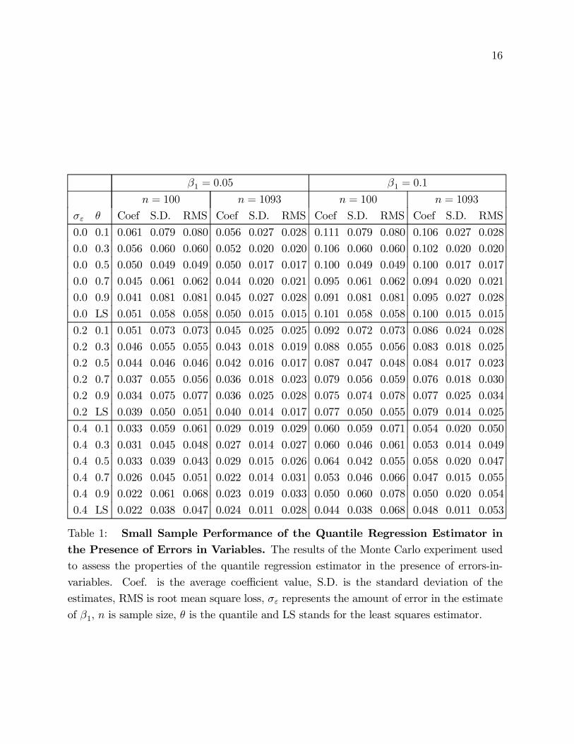
which the results for the case of EIV can be compared. The Monte Carlo output is included

in Table 1.

The results indicate that for every experiment considered, quantile regression estimates

of β1 are larger, on average, for low values of θ than for high values of θ. Where σε is

zero and the classical assumptions hold, there is a small sample bias evident in the quantile

regression estimator that is positive where θ < 0.5 and negative where θ > 0.5. For the

special case of median regression (θ = 0.5), the quantile regression estimator is unbiased

(up to a small Monte Carlo error) as expected. The bias is generally smaller for n = 1, 093

at all quantiles when compared to n = 100, demonstrating the asymptotic convergence

properties. This small sample bias deserves greater attention, which is beyond the scope

of this paper.

When EIV are induced, the shape of the function relating bias to θ is roughly equivalent

to that observed for σε = 0, that is, the average coefficient is higher for θ = 0.1 than for

θ = 0.9. In the case of EIV, however, the median regression estimator is actually less biased

than OLS and thus may be the preferred estimator when dealing with the EIV problem.

When θ = 0.5, the improved bias of the median regression estimator means that it suffers

less squared error loss than OLS, despite being less efficient. This result provides strong

evidence that, at least for the present problem, median regression is a better estimator than

OLS.18

When the EIV problem is rendered more extreme by considering σε = 0.4, the bias of

the quantile regression estimator is less than for OLS even when θ > 0.5. For n = 100,

β1 = 0.1, the bias of the OLS estimator exceeds that of the quantile estimator for all θ under

consideration. The same experiments were run for the case where β1 = −0.05 and −0.1and the results were found to be qualitatively the same but the direction of the attenuation

bias was still towards zero. The effect of the bias means that the quantile plot (the plot of

βθ against θ) will generally be flatter than it is in reality,19 i.e. patterns will appear to be

less extreme in the sample than they are in the population.

There is evidence that the plot of the bias of the quantile regression estimator against θ

‘flattens out’ as n is increased to 1,093. This finding was confirmed by a small experiment

involving pooled cross sections, suggesting that pooling is favored relative to methods based

on combining individual cross sections. Since we use pooling in this paper, interquantile

variation solely due to bias differences across θ can be ruled out.

5. Results and Discussion

The results of the empirical analysis are contained in Tables 2 through 8 and Figures 1

through 12. The general conclusion that can be drawn is that there exist wide disparities

18This point demands further consideration, including a treatment of the relevant asymptotic theory.19A useful way to think of this is to consider a case where the coefficient changes sign, say from negative

to positive. The negative estimate is attenuated and so is the positive estimate.

16

β1 = 0.05 β1 = 0.1

n = 100 n = 1093 n = 100 n = 1093

σε θ Coef S.D. RMS Coef S.D. RMS Coef S.D. RMS Coef S.D. RMS

0.0 0.1 0.061 0.079 0.080 0.056 0.027 0.028 0.111 0.079 0.080 0.106 0.027 0.028

0.0 0.3 0.056 0.060 0.060 0.052 0.020 0.020 0.106 0.060 0.060 0.102 0.020 0.020

0.0 0.5 0.050 0.049 0.049 0.050 0.017 0.017 0.100 0.049 0.049 0.100 0.017 0.017

0.0 0.7 0.045 0.061 0.062 0.044 0.020 0.021 0.095 0.061 0.062 0.094 0.020 0.021

0.0 0.9 0.041 0.081 0.081 0.045 0.027 0.028 0.091 0.081 0.081 0.095 0.027 0.028

0.0 LS 0.051 0.058 0.058 0.050 0.015 0.015 0.101 0.058 0.058 0.100 0.015 0.015

0.2 0.1 0.051 0.073 0.073 0.045 0.025 0.025 0.092 0.072 0.073 0.086 0.024 0.028

0.2 0.3 0.046 0.055 0.055 0.043 0.018 0.019 0.088 0.055 0.056 0.083 0.018 0.025

0.2 0.5 0.044 0.046 0.046 0.042 0.016 0.017 0.087 0.047 0.048 0.084 0.017 0.023

0.2 0.7 0.037 0.055 0.056 0.036 0.018 0.023 0.079 0.056 0.059 0.076 0.018 0.030

0.2 0.9 0.034 0.075 0.077 0.036 0.025 0.028 0.075 0.074 0.078 0.077 0.025 0.034

0.2 LS 0.039 0.050 0.051 0.040 0.014 0.017 0.077 0.050 0.055 0.079 0.014 0.025

0.4 0.1 0.033 0.059 0.061 0.029 0.019 0.029 0.060 0.059 0.071 0.054 0.020 0.050

0.4 0.3 0.031 0.045 0.048 0.027 0.014 0.027 0.060 0.046 0.061 0.053 0.014 0.049

0.4 0.5 0.033 0.039 0.043 0.029 0.015 0.026 0.064 0.042 0.055 0.058 0.020 0.047

0.4 0.7 0.026 0.045 0.051 0.022 0.014 0.031 0.053 0.046 0.066 0.047 0.015 0.055

0.4 0.9 0.022 0.061 0.068 0.023 0.019 0.033 0.050 0.060 0.078 0.050 0.020 0.054

0.4 LS 0.022 0.038 0.047 0.024 0.011 0.028 0.044 0.038 0.068 0.048 0.011 0.053

Table 1: Small Sample Performance of the Quantile Regression Estimator inthe Presence of Errors in Variables. The results of the Monte Carlo experiment usedto assess the properties of the quantile regression estimator in the presence of errors-in-

variables. Coef. is the average coefficient value, S.D. is the standard deviation of the

estimates, RMS is root mean square loss, σε represents the amount of error in the estimate

of β1, n is sample size, θ is the quantile and LS stands for the least squares estimator.

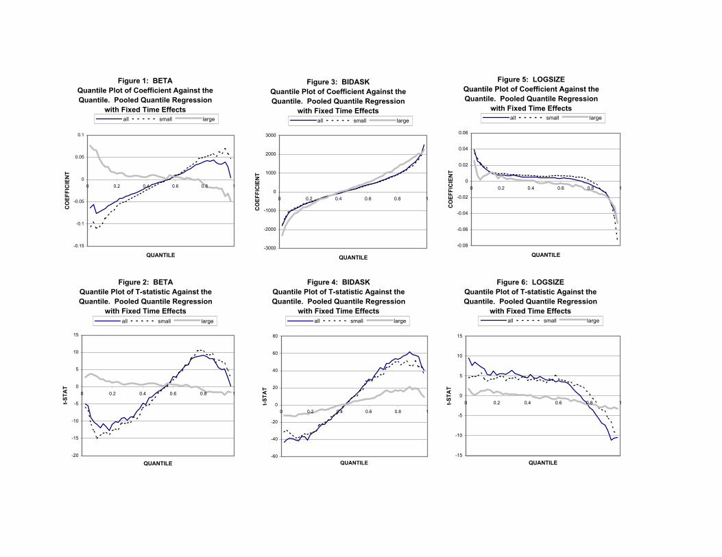
Figure 1: BETAQuantile Plot of Coefficient Against the Quantile. Pooled Quantile Regression

with Fixed Time Effects

-0.15

-0.1

-0.05

0

0.05

0.1

0 0.2 0.4 0.6 0.8 1

QUANTILE

CO

EFFI

CIE

NT

all small large

Figure 3: BIDASKQuantile Plot of Coefficient Against the Quantile. Pooled Quantile Regression

with Fixed Time Effects

-3000

-2000

-1000

0

1000

2000

3000

0 0.2 0.4 0.6 0.8 1

QUANTILEC

OEF

FIC

IEN

T

all small large

Figure 2: BETAQuantile Plot of T-statistic Against the Quantile. Pooled Quantile Regression

with Fixed Time Effects

-20

-15

-10

-5

0

5

10

15

0 0.2 0.4 0.6 0.8 1

QUANTILE

t-STA

T

all small large

Figure 4: BIDASKQuantile Plot of T-statistic Against the Quantile. Pooled Quantile Regression

with Fixed Time Effects

-60

-40

-20

0

20

40

60

80

0 0.2 0.4 0.6 0.8 1

QUANTILE

t-STA

T

all small large

Figure 6: LOGSIZEQuantile Plot of T-statistic Against the Quantile. Pooled Quantile Regression

with Fixed Time Effects

-15

-10

-5

0

5

10

15

0 0.2 0.4 0.6 0.8 1

QUANTILE

t-STA

T

all small large

Figure 5: LOGSIZEQuantile Plot of Coefficient Against the Quantile. Pooled Quantile Regression

with Fixed Time Effects

-0.08

-0.06

-0.04

-0.02

0

0.02

0.04

0.06

0 0.2 0.4 0.6 0.8 1

QUANTILE

CO

EFFI

CIE

NT

all small large

17

in behavior between underperforming and overperforming stocks, or firms that may be

receiving negative or positive idiosyncratic shocks, and that such behavior differs for large

as opposed to small firms. The quantile regression technique therefore provides considerable

insight that cannot be obtained by using standard regression techniques.

Although focusing this results section on the two-pass efficient-weighted quantile regres-

sion results for the 36 individual cross sections would provide greater conceptual compa-

rability with the existing literature, we choose to focus our discussion on the results for

the pooled, fixed time effects quantile regressions for the following reasons: 1) The in-

terquantile F-test of equality of coefficients is easily interpretable and need not be averaged

over 36 cross sections; 2) Greater sample size and degrees of freedom improve the preci-

sion of estimates; 3) Monte Carlo evidence suggesting that larger samples display more

evenly-distributed attenuation bias across quantiles than observed for smaller samples; and

4) Both approaches yield qualitatively similar results.

Reported p-values are constructed using the design matrix bootstrap approach and hence

are robust to serial correlation, heteroskedasticity and any general dependence between the

regressors and the regression errors. Throughout this section, we primarily discuss the

pooled results but note any discrepancies between the results from the two levels of pooling.

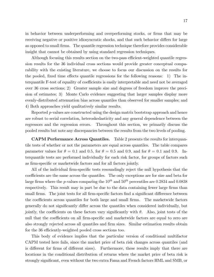
CAPMPerformance Across Quantiles. Table 2 presents the results for interquan-

tile tests of whether or not the parameters are equal across quantiles. The table compares

parameter values for θ = 0.1 and 0.5, for θ = 0.5 and 0.9, and for θ = 0.1 and 0.9. In-

terquantile tests are performed individually for each risk factor, for groups of factors such

as firm-specific or marketwide factors and for all factors jointly.

All of the individual firm-specific tests resoundingly reject the null hypothesis that the

coefficients are the same across the quantiles. The only exceptions are for size and beta for

large firms where the p-values comparing the 10th and 50th percentiles are 0.2834 and 0.0838

respectively. This result may in part be due to the data containing fewer large firms than

small firms. The joint tests for all firm-specific factors find a significant difference between

the coefficients across quantiles for both large and small firms. The marketwide factors

generally do not significantly differ across the quantiles when considered individually, but

jointly, the coefficients on these factors vary significantly with θ. Also, joint tests of the

null that the coefficients on all firm-specific and marketwide factors are equal to zero are

also strongly rejected across all quantiles and firm sizes. Similar estimation results obtain

for the 36 efficiently-weighted pooled cross sections too.

This body of evidence implies that the particular version of conditional multifactor

CAPM tested here fails, since the market price of beta risk changes across quantiles (and

is different for firms of different sizes). Furthermore, these results imply that there are

locations in the conditional distribution of returns where the market price of beta risk is

strongly significant, even without the two extra Fama and French factors HML and SMB, or

18

ALL ddof = 39303 SMALL ddof = 30123 BIG ddof = 9135

10-50 50-90 10-90 10-50 50-90 10-90 10-50 50-90 10-90

beta 65.88 19.69 84.62 120.47 46.44 171.98 2.99 2.97 6.62

ndof=1 0.0000 0.0000 0.0000 0.0000 0.0000 0.0000 0.0838 0.0850 0.0101

bidask 600.48 656.79 1281.33 967.32 445.58 1273.29 142.93 187.77 444.75

ndof=1 0.0000 0.0000 0.0000 0.0000 0.0000 0.0000 0.0000 0.0000 0.0000

logsize 30.87 127.75 148.06 12.25 30.37 62.51 1.15 6.81 6.33

ndof=1 0.0000 0.0000 0.0000 0.0005 0.0000 0.0000 0.2834 0.0091 0.0119

finp 0.43 0.83 0.07 1.35 0.60 0.03 0.90 1.66 2.67

ndof=1 0.5107 0.3623 0.7889 0.2446 0.4370 0.8532 0.3423 0.1980 0.1025

junk 0.15 0.02 0.14 0.01 0.49 0.39 0.00 3.91 2.26

ndof=1 0.6989 0.8800 0.7079 0.9186 0.4846 0.5330 0.9574 0.0481 0.1327

mnt3 0.21 0.10 0.00 0.54 0.00 0.20 0.09 0.89 0.23

ndof=1 0.6454 0.7512 0.9616 0.4610 0.9490 0.6546 0.7668 0.3442 0.6315

mnt6 0.95 0.37 1.54 1.33 0.25 1.38 0.27 1.16 1.53

ndof=1 0.3297 0.5441 0.2142 0.2489 0.6149 0.2398 0.6036 0.2825 0.2159

slfh 0.00 0.29 0.21 0.05 0.26 0.32 0.36 0.23 0.07

ndof=1 0.9968 0.5877 0.6482 0.8217 0.6108 0.5701 0.5507 0.6324 0.7945

term 5.75 0.02 2.90 2.26 0.00 0.89 2.23 0.82 3.17

ndof=1 0.0165 0.8805 0.0888 0.1331 0.9679 0.3460 0.1353 0.3656 0.0751

FS-MW 110.50 135.44 256.08 161.29 84.40 226.54 24.30 31.24 79.12

ndof=9 0.0000 0.0000 0.0000 0.0000 0.0000 0.0000 0.0000 0.0000 0.0000

FS 323.97 386.70 661.17 471.61 218.17 588.88 64.67 89.00 233.73

ndof=3 0.0000 0.0000 0.0000 0.0000 0.0000 0.0000 0.0000 0.0000 0.0000

MW 3.57 0.42 2.89 2.88 0.40 1.23 2.39 1.26 3.79

ndof=6 0.0015 0.8644 0.0081 0.0083 0.8780 0.2887 0.0264 0.2701 0.0009

Table 2: Individual and Joint Interquantile Tests Using Pooled Quantile Regres-sions. Individual and joint interquantile tests based on pooled quantile regressions withtime-specific fixed effects. We include F-statistics and p-values. The p-values are based

on the F-distribution with the stated number of numerator (ndof) and denominator (ddof)

degrees of freedom. FS-MW is a joint test of whether firm-specific and marketwide factors

are constant across the stated quantiles; FS tests just the firm-specific factors; and MW

tests just the marketwide factors. ALL represents the case where all firms are included in

the data set; SMALL includes only firms with lower than average market capitalization;

and BIG includes only larger than average firms. 10 − 50 indicates that the test is for de-termining whether or not the coefficients differ across the 10th and 50th quantiles; 50− 90indicates the test is for the 50th and 90th quantiles; and 10 − 90 indicates the test is fordetermining whether the coefficients differ across the 10th and 90th quantiles.

19

other factors that have typically helped to resuscitate the CAPM. Since it is the case that

we can reject the hypothesis that the coefficients are the same across quantiles, we find that

none of the empirical or theoretical results previously uncovered in the literature (positive,

negative or zero market prices of risk) are supported unambiguously. By construction, we

show that the results obtained using LS-based methods are but one perspective on the more

complex set of patterns revealed by quantile regression.

Firm-Specific Conditional Variables. Theory says that returns should increase

with beta, so we would expect a positive and significant coefficient on the market price of

beta risk across all quantiles. Furthermore, the expected return for an individual firm should

share the same market price of risk as all firms in equilibrium. Above, we showed that the

market price of risk is not the same across all firms. Here, by inspection of the coefficients

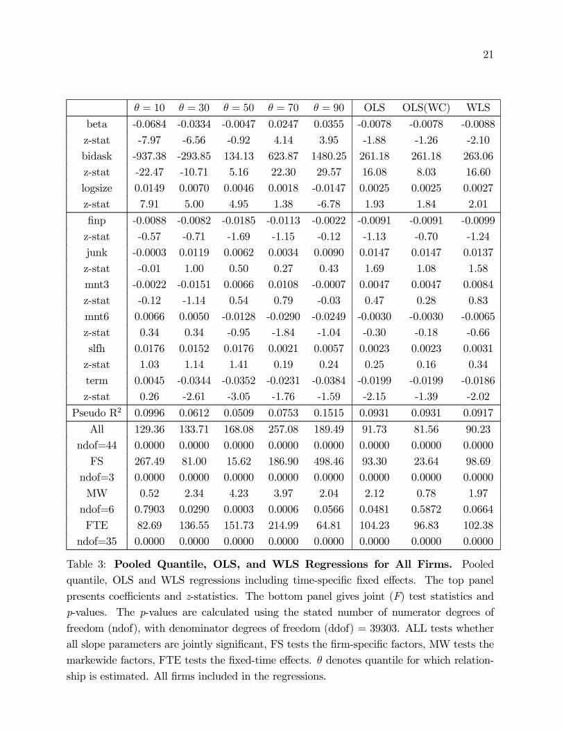
and t-statistics from the pooled quantile regression in Figures 1 and 2 and in Tables 3

through 5, we reveal that beta is not a significant explanator of returns across the entire

conditional distribution. In general, an “S” pattern is observed, where beta has a negative

coefficient for firms that underperform the mean (or have a negative idiosyncratic shock or

bad news) and a positive coefficient for firms that overperform the mean. In particular,

beta is significant and positive for the top 30% of firms, implying that the theoretical CAPM

relationship applies conditionally, but only for firms that out-perform the mean. Firms in

the lower quantiles have unobserved characteristics that are not conducive to high returns.

The market appears to price these assets in such a way that there is a significant negative

return to beta risk. Moving across the quantiles, the quality of the unobserved factors

improves and the effect of additional beta risk becomes positive. An interesting result here

is the negative slope that occurs in the quantile plot in the upper 25% of the distribution.

This implies that in this range, as the unobserved factors improve, firms experience a lower

return to increased beta risk.

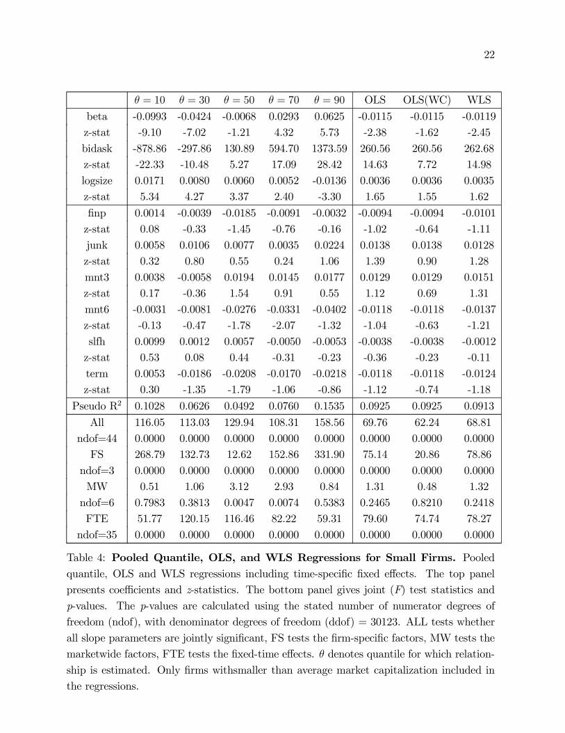
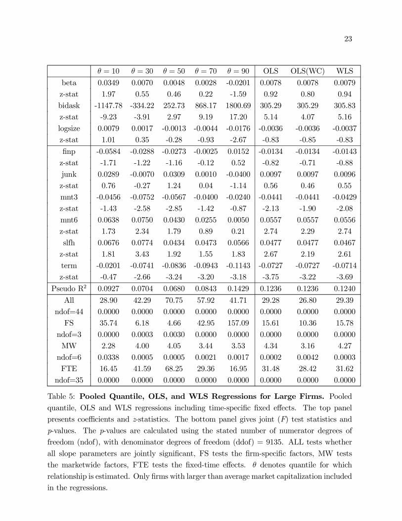
The opposing results for large and small firms are striking. As the unobserved factors

improve, the return to beta risk for large firms decreases, suggesting that the market places

a positive price on beta risk for large firms that receive negative idiosyncratic shocks or are

underperforming and a negative price on this risk for overperforming or good-news large

firms. On the contrary, for small firms that are underperforming, the price of beta risk

is negative while for overperforming small firms, the market price of beta risk is positive.

Small firms are dominating the overall pattern in the quantile plot, as the majority that

are included in our sample are small. Not surprisingly, around the center of the distribu-

tion, the coefficients lie on either side of zero without statistical significance, underscoring

the ambiguous results typically found in the literature where the mean is the only point

considered.20

20The differences between the results for large and small firms may be due to the fact that the excessmarket return, and hence beta risk, is largely constituted by large firms. Perhaps if the market return were

20

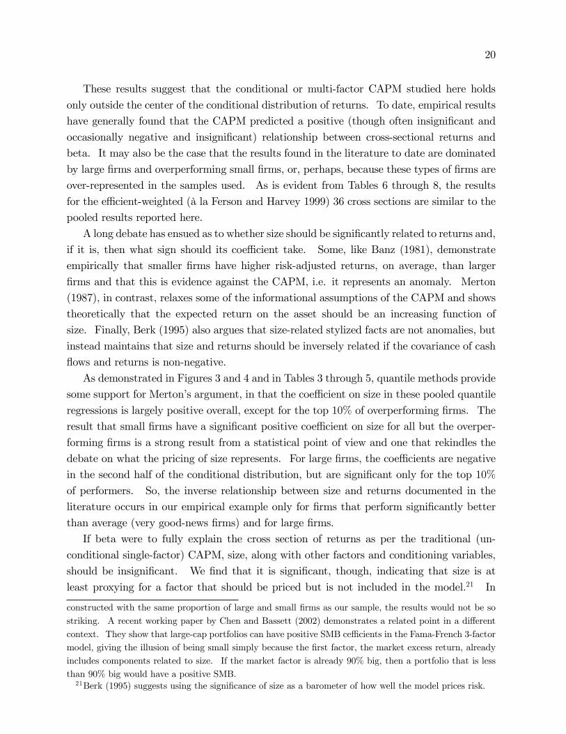
These results suggest that the conditional or multi-factor CAPM studied here holds

only outside the center of the conditional distribution of returns. To date, empirical results

have generally found that the CAPM predicted a positive (though often insignificant and

occasionally negative and insignificant) relationship between cross-sectional returns and

beta. It may also be the case that the results found in the literature to date are dominated

by large firms and overperforming small firms, or, perhaps, because these types of firms are

over-represented in the samples used. As is evident from Tables 6 through 8, the results

for the efficient-weighted (à la Ferson and Harvey 1999) 36 cross sections are similar to the

pooled results reported here.

A long debate has ensued as to whether size should be significantly related to returns and,

if it is, then what sign should its coefficient take. Some, like Banz (1981), demonstrate

empirically that smaller firms have higher risk-adjusted returns, on average, than larger

firms and that this is evidence against the CAPM, i.e. it represents an anomaly. Merton

(1987), in contrast, relaxes some of the informational assumptions of the CAPM and shows

theoretically that the expected return on the asset should be an increasing function of

size. Finally, Berk (1995) also argues that size-related stylized facts are not anomalies, but

instead maintains that size and returns should be inversely related if the covariance of cash

flows and returns is non-negative.

As demonstrated in Figures 3 and 4 and in Tables 3 through 5, quantile methods provide

some support for Merton’s argument, in that the coefficient on size in these pooled quantile

regressions is largely positive overall, except for the top 10% of overperforming firms. The

result that small firms have a significant positive coefficient on size for all but the overper-

forming firms is a strong result from a statistical point of view and one that rekindles the

debate on what the pricing of size represents. For large firms, the coefficients are negative

in the second half of the conditional distribution, but are significant only for the top 10%

of performers. So, the inverse relationship between size and returns documented in the

literature occurs in our empirical example only for firms that perform significantly better

than average (very good-news firms) and for large firms.

If beta were to fully explain the cross section of returns as per the traditional (un-

conditional single-factor) CAPM, size, along with other factors and conditioning variables,

should be insignificant. We find that it is significant, though, indicating that size is at

least proxying for a factor that should be priced but is not included in the model.21 In

constructed with the same proportion of large and small firms as our sample, the results would not be sostriking. A recent working paper by Chen and Bassett (2002) demonstrates a related point in a differentcontext. They show that large-cap portfolios can have positive SMB cefficients in the Fama-French 3-factormodel, giving the illusion of being small simply because the first factor, the market excess return, alreadyincludes components related to size. If the market factor is already 90% big, then a portfolio that is lessthan 90% big would have a positive SMB.21Berk (1995) suggests using the significance of size as a barometer of how well the model prices risk.

21

θ = 10 θ = 30 θ = 50 θ = 70 θ = 90 OLS OLS(WC) WLS

beta -0.0684 -0.0334 -0.0047 0.0247 0.0355 -0.0078 -0.0078 -0.0088

z-stat -7.97 -6.56 -0.92 4.14 3.95 -1.88 -1.26 -2.10

bidask -937.38 -293.85 134.13 623.87 1480.25 261.18 261.18 263.06

z-stat -22.47 -10.71 5.16 22.30 29.57 16.08 8.03 16.60

logsize 0.0149 0.0070 0.0046 0.0018 -0.0147 0.0025 0.0025 0.0027

z-stat 7.91 5.00 4.95 1.38 -6.78 1.93 1.84 2.01

finp -0.0088 -0.0082 -0.0185 -0.0113 -0.0022 -0.0091 -0.0091 -0.0099

z-stat -0.57 -0.71 -1.69 -1.15 -0.12 -1.13 -0.70 -1.24

junk -0.0003 0.0119 0.0062 0.0034 0.0090 0.0147 0.0147 0.0137

z-stat -0.01 1.00 0.50 0.27 0.43 1.69 1.08 1.58

mnt3 -0.0022 -0.0151 0.0066 0.0108 -0.0007 0.0047 0.0047 0.0084

z-stat -0.12 -1.14 0.54 0.79 -0.03 0.47 0.28 0.83

mnt6 0.0066 0.0050 -0.0128 -0.0290 -0.0249 -0.0030 -0.0030 -0.0065

z-stat 0.34 0.34 -0.95 -1.84 -1.04 -0.30 -0.18 -0.66

slfh 0.0176 0.0152 0.0176 0.0021 0.0057 0.0023 0.0023 0.0031

z-stat 1.03 1.14 1.41 0.19 0.24 0.25 0.16 0.34

term 0.0045 -0.0344 -0.0352 -0.0231 -0.0384 -0.0199 -0.0199 -0.0186

z-stat 0.26 -2.61 -3.05 -1.76 -1.59 -2.15 -1.39 -2.02

Pseudo R2 0.0996 0.0612 0.0509 0.0753 0.1515 0.0931 0.0931 0.0917

All 129.36 133.71 168.08 257.08 189.49 91.73 81.56 90.23

ndof=44 0.0000 0.0000 0.0000 0.0000 0.0000 0.0000 0.0000 0.0000

FS 267.49 81.00 15.62 186.90 498.46 93.30 23.64 98.69

ndof=3 0.0000 0.0000 0.0000 0.0000 0.0000 0.0000 0.0000 0.0000

MW 0.52 2.34 4.23 3.97 2.04 2.12 0.78 1.97

ndof=6 0.7903 0.0290 0.0003 0.0006 0.0566 0.0481 0.5872 0.0664

FTE 82.69 136.55 151.73 214.99 64.81 104.23 96.83 102.38

ndof=35 0.0000 0.0000 0.0000 0.0000 0.0000 0.0000 0.0000 0.0000

Table 3: Pooled Quantile, OLS, and WLS Regressions for All Firms. Pooled

quantile, OLS and WLS regressions including time-specific fixed effects. The top panel

presents coefficients and z-statistics. The bottom panel gives joint (F) test statistics and

p-values. The p-values are calculated using the stated number of numerator degrees of

freedom (ndof), with denominator degrees of freedom (ddof) = 39303. ALL tests whether

all slope parameters are jointly significant, FS tests the firm-specific factors, MW tests the

markewide factors, FTE tests the fixed-time effects. θ denotes quantile for which relation-

ship is estimated. All firms included in the regressions.

22

θ = 10 θ = 30 θ = 50 θ = 70 θ = 90 OLS OLS(WC) WLS

beta -0.0993 -0.0424 -0.0068 0.0293 0.0625 -0.0115 -0.0115 -0.0119

z-stat -9.10 -7.02 -1.21 4.32 5.73 -2.38 -1.62 -2.45

bidask -878.86 -297.86 130.89 594.70 1373.59 260.56 260.56 262.68

z-stat -22.33 -10.48 5.27 17.09 28.42 14.63 7.72 14.98

logsize 0.0171 0.0080 0.0060 0.0052 -0.0136 0.0036 0.0036 0.0035

z-stat 5.34 4.27 3.37 2.40 -3.30 1.65 1.55 1.62

finp 0.0014 -0.0039 -0.0185 -0.0091 -0.0032 -0.0094 -0.0094 -0.0101

z-stat 0.08 -0.33 -1.45 -0.76 -0.16 -1.02 -0.64 -1.11

junk 0.0058 0.0106 0.0077 0.0035 0.0224 0.0138 0.0138 0.0128

z-stat 0.32 0.80 0.55 0.24 1.06 1.39 0.90 1.28

mnt3 0.0038 -0.0058 0.0194 0.0145 0.0177 0.0129 0.0129 0.0151

z-stat 0.17 -0.36 1.54 0.91 0.55 1.12 0.69 1.31

mnt6 -0.0031 -0.0081 -0.0276 -0.0331 -0.0402 -0.0118 -0.0118 -0.0137

z-stat -0.13 -0.47 -1.78 -2.07 -1.32 -1.04 -0.63 -1.21

slfh 0.0099 0.0012 0.0057 -0.0050 -0.0053 -0.0038 -0.0038 -0.0012

z-stat 0.53 0.08 0.44 -0.31 -0.23 -0.36 -0.23 -0.11

term 0.0053 -0.0186 -0.0208 -0.0170 -0.0218 -0.0118 -0.0118 -0.0124

z-stat 0.30 -1.35 -1.79 -1.06 -0.86 -1.12 -0.74 -1.18

Pseudo R2 0.1028 0.0626 0.0492 0.0760 0.1535 0.0925 0.0925 0.0913

All 116.05 113.03 129.94 108.31 158.56 69.76 62.24 68.81

ndof=44 0.0000 0.0000 0.0000 0.0000 0.0000 0.0000 0.0000 0.0000

FS 268.79 132.73 12.62 152.86 331.90 75.14 20.86 78.86

ndof=3 0.0000 0.0000 0.0000 0.0000 0.0000 0.0000 0.0000 0.0000

MW 0.51 1.06 3.12 2.93 0.84 1.31 0.48 1.32

ndof=6 0.7983 0.3813 0.0047 0.0074 0.5383 0.2465 0.8210 0.2418

FTE 51.77 120.15 116.46 82.22 59.31 79.60 74.74 78.27

ndof=35 0.0000 0.0000 0.0000 0.0000 0.0000 0.0000 0.0000 0.0000

Table 4: Pooled Quantile, OLS, and WLS Regressions for Small Firms. Pooledquantile, OLS and WLS regressions including time-specific fixed effects. The top panel

presents coefficients and z-statistics. The bottom panel gives joint (F) test statistics and

p-values. The p-values are calculated using the stated number of numerator degrees of

freedom (ndof), with denominator degrees of freedom (ddof) = 30123. ALL tests whether

all slope parameters are jointly significant, FS tests the firm-specific factors, MW tests the

marketwide factors, FTE tests the fixed-time effects. θ denotes quantile for which relation-

ship is estimated. Only firms withsmaller than average market capitalization included in

the regressions.

23

θ = 10 θ = 30 θ = 50 θ = 70 θ = 90 OLS OLS(WC) WLS

beta 0.0349 0.0070 0.0048 0.0028 -0.0201 0.0078 0.0078 0.0079

z-stat 1.97 0.55 0.46 0.22 -1.59 0.92 0.80 0.94

bidask -1147.78 -334.22 252.73 868.17 1800.69 305.29 305.29 305.83

z-stat -9.23 -3.91 2.97 9.19 17.20 5.14 4.07 5.16

logsize 0.0079 0.0017 -0.0013 -0.0044 -0.0176 -0.0036 -0.0036 -0.0037

z-stat 1.01 0.35 -0.28 -0.93 -2.67 -0.83 -0.85 -0.83

finp -0.0584 -0.0288 -0.0273 -0.0025 0.0152 -0.0134 -0.0134 -0.0143

z-stat -1.71 -1.22 -1.16 -0.12 0.52 -0.82 -0.71 -0.88

junk 0.0289 -0.0070 0.0309 0.0010 -0.0400 0.0097 0.0097 0.0096

z-stat 0.76 -0.27 1.24 0.04 -1.14 0.56 0.46 0.55

mnt3 -0.0456 -0.0752 -0.0567 -0.0400 -0.0240 -0.0441 -0.0441 -0.0429

z-stat -1.43 -2.58 -2.85 -1.42 -0.87 -2.13 -1.90 -2.08

mnt6 0.0638 0.0750 0.0430 0.0255 0.0050 0.0557 0.0557 0.0556

z-stat 1.73 2.34 1.79 0.89 0.21 2.74 2.29 2.74

slfh 0.0676 0.0774 0.0434 0.0473 0.0566 0.0477 0.0477 0.0467

z-stat 1.81 3.43 1.92 1.55 1.83 2.67 2.19 2.61

term -0.0201 -0.0741 -0.0836 -0.0943 -0.1143 -0.0727 -0.0727 -0.0714

z-stat -0.47 -2.66 -3.24 -3.20 -3.18 -3.75 -3.22 -3.69

Pseudo R2 0.0927 0.0704 0.0680 0.0843 0.1429 0.1236 0.1236 0.1240

All 28.90 42.29 70.75 57.92 41.71 29.28 26.80 29.39

ndof=44 0.0000 0.0000 0.0000 0.0000 0.0000 0.0000 0.0000 0.0000

FS 35.74 6.18 4.66 42.95 157.09 15.61 10.36 15.78

ndof=3 0.0000 0.0003 0.0030 0.0000 0.0000 0.0000 0.0000 0.0000

MW 2.28 4.00 4.05 3.44 3.53 4.34 3.16 4.27

ndof=6 0.0338 0.0005 0.0005 0.0021 0.0017 0.0002 0.0042 0.0003

FTE 16.45 41.59 68.25 29.36 16.95 31.48 28.42 31.62

ndof=35 0.0000 0.0000 0.0000 0.0000 0.0000 0.0000 0.0000 0.0000

Table 5: Pooled Quantile, OLS, and WLS Regressions for Large Firms. Pooledquantile, OLS and WLS regressions including time-specific fixed effects. The top panel

presents coefficients and z-statistics. The bottom panel gives joint (F) test statistics and

p-values. The p-values are calculated using the stated number of numerator degrees of

freedom (ndof), with denominator degrees of freedom (ddof) = 9135. ALL tests whether

all slope parameters are jointly significant, FS tests the firm-specific factors, MW tests

the marketwide factors, FTE tests the fixed-time effects. θ denotes quantile for which

relationship is estimated. Only firms with larger than average market capitalization included

in the regressions.

24

θ = 10 θ = 30 θ = 50 θ = 70 θ = 90 EOLS EOLS(WC) EWLS

beta -0.0508 -0.0273 -0.0060 0.0208 0.0414 -0.0042 -0.0052 -0.0051

z-stat -5.97 -4.61 -1.10 3.50 4.34 -0.95 -0.86 -1.16

bidask -764.42 -301.56 92.11 523.33 1213.37 210.31 187.19 209.94

z-stat -20.05 -10.97 3.63 17.90 26.42 12.81 6.46 13.14

logsize 0.0133 0.0040 0.0036 0.0026 -0.0122 0.0034 0.0038 0.0038

z-stat 7.18 3.28 3.26 2.17 -5.97 2.63 2.93 2.90

finp -0.0385 -0.0064 -0.0278 0.0078 0.0142 -0.0066 -0.0039 -0.0107

z-stat -1.53 -0.32 -1.48 0.38 0.50 -0.47 -0.19 -0.77

junk -0.0117 -0.0046 -0.0205 0.0065 0.0098 0.0178 0.0068 0.0211

z-stat -0.45 -0.26 -1.21 0.34 0.35 1.36 0.36 1.61

mnt3 0.0602 0.0551 0.0466 0.0256 0.0377 0.0457 0.0396 0.0505

z-stat 1.89 2.53 1.98 0.95 1.00 2.57 1.51 2.85

mnt6 0.0091 -0.0161 -0.0276 -0.0665 -0.0734 -0.0447 -0.0311 -0.0492

z-stat 0.23 -0.66 -1.10 -2.26 -1.77 -2.36 -1.10 -2.60

slfh -0.0401 -0.0014 0.0133 0.0047 0.0457 0.0020 0.0034 -0.0015

z-stat -0.98 -0.05 0.51 0.16 1.06 0.10 0.11 -0.07

term 0.0726 -0.0309 -0.0153 -0.0064 -0.0004 -0.0129 -0.0103 -0.0148

z-stat 2.07 -1.22 -0.62 -0.23 -0.01 -0.72 -0.40 -0.83

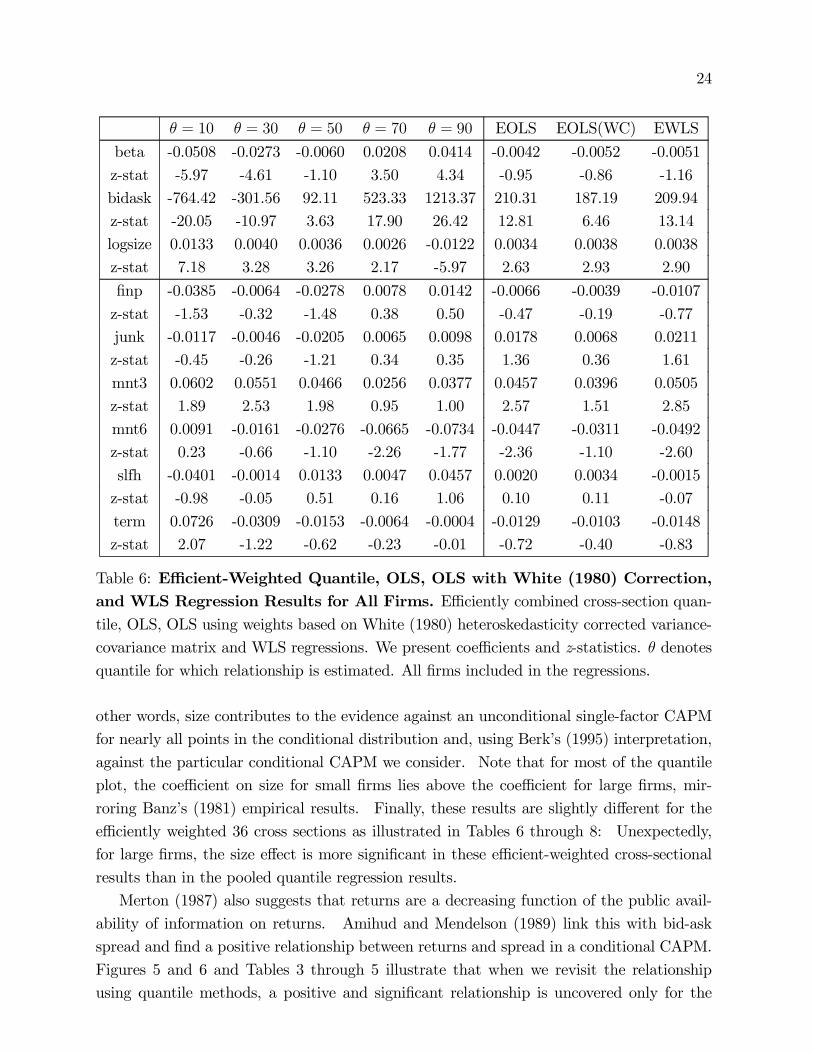
Table 6: Efficient-Weighted Quantile, OLS, OLS with White (1980) Correction,and WLS Regression Results for All Firms. Efficiently combined cross-section quan-tile, OLS, OLS using weights based on White (1980) heteroskedasticity corrected variance-

covariance matrix and WLS regressions. We present coefficients and z-statistics. θ denotes

quantile for which relationship is estimated. All firms included in the regressions.

other words, size contributes to the evidence against an unconditional single-factor CAPM

for nearly all points in the conditional distribution and, using Berk’s (1995) interpretation,

against the particular conditional CAPM we consider. Note that for most of the quantile

plot, the coefficient on size for small firms lies above the coefficient for large firms, mir-

roring Banz’s (1981) empirical results. Finally, these results are slightly different for the

efficiently weighted 36 cross sections as illustrated in Tables 6 through 8: Unexpectedly,

for large firms, the size effect is more significant in these efficient-weighted cross-sectional

results than in the pooled quantile regression results.

Merton (1987) also suggests that returns are a decreasing function of the public avail-

ability of information on returns. Amihud and Mendelson (1989) link this with bid-ask

spread and find a positive relationship between returns and spread in a conditional CAPM.

Figures 5 and 6 and Tables 3 through 5 illustrate that when we revisit the relationship

using quantile methods, a positive and significant relationship is uncovered only for the

25

θ = 10 θ = 30 θ = 50 θ = 70 θ = 90 EOLS EOLS(WC) EWLS

beta -0.0793 -0.0394 -0.0026 0.0196 0.0526 -0.0084 -0.0103 -0.0087

z-stat -7.66 -5.76 -0.42 2.77 4.64 -1.66 -1.50 -1.71

bidask -788.48 -299.30 95.01 499.05 1159.32 211.07 190.79 210.46

z-stat -19.99 -11.09 3.63 16.21 24.06 11.73 6.39 11.91

logsize 0.0136 0.0050 0.0053 0.0055 -0.0088 0.0056 0.0056 0.0057

z-stat 4.05 2.75 3.12 2.86 -2.51 2.68 2.59 2.72

finp -0.0059 0.0043 -0.0210 -0.0038 0.0322 -0.0052 -0.0008 -0.0101

z-stat -0.19 0.18 -0.95 -0.17 0.90 -0.32 -0.04 -0.63

junk -0.0164 0.0078 -0.0353 0.0066 0.0274 0.0172 0.0036 0.0210

z-stat -0.57 0.39 -1.78 0.30 0.85 1.15 0.17 1.41

mnt3 0.0589 0.0636 0.0713 0.0361 0.0510 0.0483 0.0426 0.0524

z-stat 1.53 2.35 2.61 1.15 1.10 2.38 1.46 2.58

mnt6 0.0212 -0.0465 -0.0502 -0.0742 -0.0729 -0.0548 -0.0416 -0.0572

z-stat 0.50 -1.59 -1.76 -2.20 -1.53 -2.54 -1.33 -2.65

slfh -0.0582 -0.0352 0.0061 -0.0189 0.0077 -0.0093 -0.0116 -0.0097

z-stat -1.27 -1.11 0.21 -0.58 0.15 -0.41 -0.35 -0.43

term 0.0693 -0.0127 -0.0128 0.0212 0.0274 -0.0056 0.0020 -0.0096

z-stat 1.74 -0.43 -0.46 0.71 0.64 -0.27 0.07 -0.47

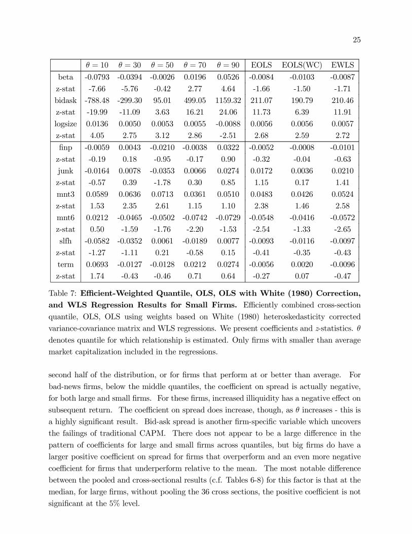
Table 7: Efficient-Weighted Quantile, OLS, OLS with White (1980) Correction,and WLS Regression Results for Small Firms. Efficiently combined cross-sectionquantile, OLS, OLS using weights based on White (1980) heteroskedasticity corrected

variance-covariance matrix and WLS regressions. We present coefficients and z-statistics. θ

denotes quantile for which relationship is estimated. Only firms with smaller than average

market capitalization included in the regressions.

second half of the distribution, or for firms that perform at or better than average. For

bad-news firms, below the middle quantiles, the coefficient on spread is actually negative,

for both large and small firms. For these firms, increased illiquidity has a negative effect on

subsequent return. The coefficient on spread does increase, though, as θ increases - this is

a highly significant result. Bid-ask spread is another firm-specific variable which uncovers

the failings of traditional CAPM. There does not appear to be a large difference in the

pattern of coefficients for large and small firms across quantiles, but big firms do have a

larger positive coefficient on spread for firms that overperform and an even more negative

coefficient for firms that underperform relative to the mean. The most notable difference

between the pooled and cross-sectional results (c.f. Tables 6-8) for this factor is that at the

median, for large firms, without pooling the 36 cross sections, the positive coefficient is not

significant at the 5% level.

26

θ = 10 θ = 30 θ = 50 θ = 70 θ = 90 EOLS EOLS(WC) EWLS

beta 0.0276 0.0166 0.0036 0.0000 -0.0322 0.0133 0.0113 0.0136

z-stat 1.58 1.33 0.30 0.00 -1.95 1.48 1.13 1.52

bidask -1073.31 -478.56 159.44 820.54 1641.88 218.55 202.89 219.84

z-stat -9.38 -5.25 1.81 9.36 13.97 3.57 2.85 3.59

logsize 0.0078 0.0028 -0.0068 -0.0094 -0.0192 -0.0049 -0.0034 -0.0050

z-stat 1.18 0.56 -1.49 -1.95 -2.96 -1.16 -0.84 -1.16

finp -0.0374 -0.0822 -0.0559 0.0207 0.0426 -0.0256 -0.0193 -0.0270

z-stat -0.71 -1.88 -1.39 0.50 0.85 -0.89 -0.60 -0.94

junk 0.0421 0.0590 0.0610 0.0002 -0.0136 0.0325 0.0441 0.0328

z-stat 0.78 1.49 1.67 0.01 -0.29 1.21 1.46 1.22

mnt3 0.0930 0.0037 -0.0279 -0.0294 -0.0764 -0.0143 -0.0067 -0.0125

z-stat 1.37 0.08 -0.57 -0.61 -1.22 -0.40 -0.18 -0.35

mnt6 -0.0875 0.0871 0.0520 0.0316 0.0607 0.0456 0.0325 0.0450

z-stat -0.96 1.50 0.98 0.60 0.90 1.14 0.73 1.12

slfh -0.0185 0.0817 0.0894 0.1137 0.1265 0.0909 0.0929 0.0874

z-stat -0.24 1.31 1.61 1.90 1.70 2.14 1.87 2.06

term -0.0185 -0.1391 -0.0952 -0.0999 -0.1012 -0.0795 -0.0843 -0.0767

z-stat -0.26 -2.66 -1.73 -1.62 -1.48 -2.04 -1.93 -1.97

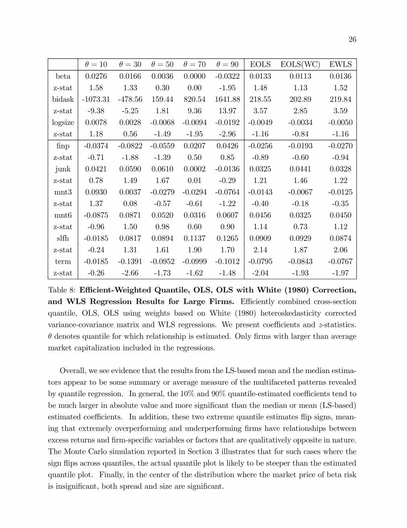
Table 8: Efficient-Weighted Quantile, OLS, OLS with White (1980) Correction,and WLS Regression Results for Large Firms. Efficiently combined cross-sectionquantile, OLS, OLS using weights based on White (1980) heteroskedasticity corrected

variance-covariance matrix and WLS regressions. We present coefficients and z-statistics.

θ denotes quantile for which relationship is estimated. Only firms with larger than average

market capitalization included in the regressions.

Overall, we see evidence that the results from the LS-based mean and the median estima-

tors appear to be some summary or average measure of the multifaceted patterns revealed

by quantile regression. In general, the 10% and 90% quantile-estimated coefficients tend to

be much larger in absolute value and more significant than the median or mean (LS-based)

estimated coefficients. In addition, these two extreme quantile estimates flip signs, mean-

ing that extremely overperforming and underperforming firms have relationships between

excess returns and firm-specific variables or factors that are qualitatively opposite in nature.

The Monte Carlo simulation reported in Section 3 illustrates that for such cases where the

sign flips across quantiles, the actual quantile plot is likely to be steeper than the estimated

quantile plot. Finally, in the center of the distribution where the market price of beta risk

is insignificant, both spread and size are significant.

27

Marketwide Factors. Numerous authors, including Breen, Glosten and Jagannathan

(1989), Ferson and Harvey (1991) and Campbell (1987) follow the Fama and Schwert (1977)

tradition and find a negative relationship between returns and financial paper (finp). It is

clear from the quantile plot of the t-statistics (Figure 7) and from Tables 3 through 5

that this pattern is significant for large firms only in the bottom 10% of the conditional

distribution for the empirical example considered here.22 Small firms tend to exhibit a

negative partial correlation between these variables for the top 70% of conditional returns,

but the coefficients are largely insignificant. Overall, the small firms appear to dominate the

pattern of the quantile plot since our sample largely consists of small firms. This negative

relationship is significant at the median for all firms at the 10% level of significance.

In Figure 8, the quantile plot for the t-statistic on the coefficient on the three-month

yield spread factor (mnt3), a measure of the short-maturity term structure, shows very little

substantiating evidence for the Harvey (1989) and Ferson and Harvey (1991) predictions

of a positive relationship between the three-month yield spread and returns. Mostly, the

results indicate that there tends to be a positive but largely insignificant relationship for

small firms (with some statistical significance around the center of the distribution) and

a negative relationship for large firms which is significant at or just below the median (at

the 30% and 50% quantiles). This is corroborated by the results in Tables 3 through 5.

In contrast, Figure 9 demonstrates that for the six-month yield spread (mnt6), another

measure of the term structure used by Campbell (1987), the coefficient is positive almost

everywhere for large firms, and is generally significant for the first 50% of the conditional

distribution. For small firms, the coefficient is largely insignificant (except for the 50% and

70% quantiles) and negative.

The default or junk bond premium, or the spread between Moody’s Aaa and Baa yields

(junk), is used as a measure of business conditions by Fama and French (1989) and as a

measure of changes in the risk of corporate default by Ferson and Harvey (1991). Both

of these studies find empirical support for a positive relationship between returns and the

junk premium. Fama and French (1989) argue that the default premium captures time

variation in expected stock returns as a result of changes in business conditions that endure

longer than business cycles. They find that the default premium moves in opposition to

business conditions, and argue that returns move in a similar way using a consumption-

smoothing argument. They also note that some consumption-smoothing-based arguments

yield the opposite prediction. From Figure 10 and Tables 3 through 5 it is apparent that

their positive prediction holds true across most of the quantile plot for both large and small

firms. However, in this empirical example, this is not a significant result. In fact, the only

(slightly) significant results obtain for small and large firms in the 50th percentile for the

22The extensive literature on the Fisher hypothesis in the context of stock returns demonstrates that suchresults can be sensitive to data frequency, so the results here may differ from those found in the literaturedue to our choice of data frequency.

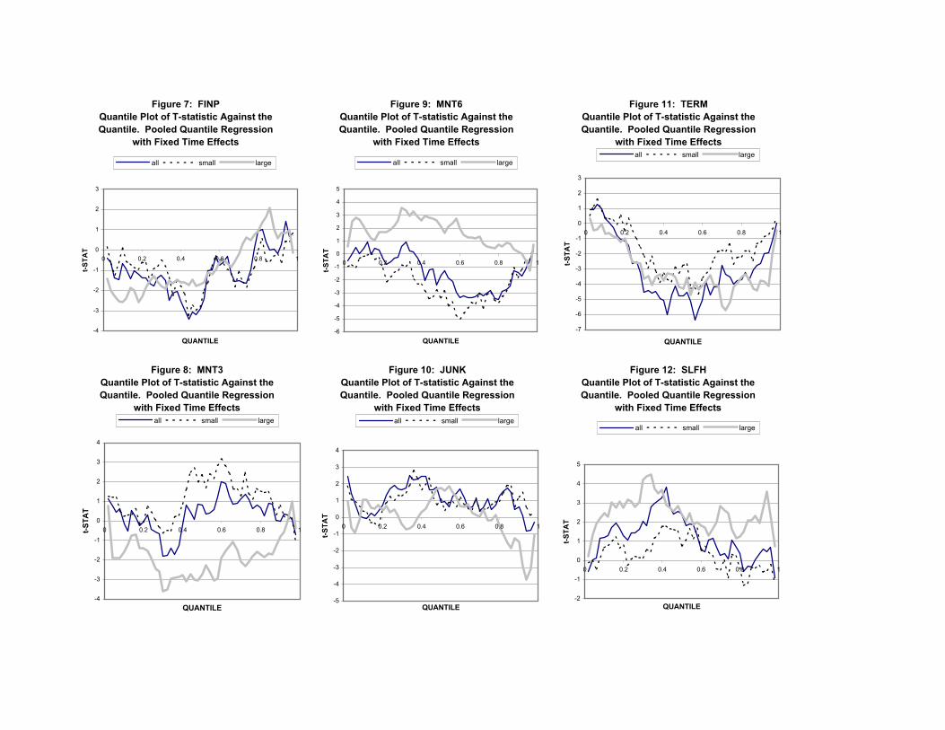
Figure 7: FINPQuantile Plot of T-statistic Against the Quantile. Pooled Quantile Regression

with Fixed Time Effects

-4

-3

-2

-1

0

1

2

3

0 0.2 0.4 0.6 0.8 1

QUANTILE

t-STA

T

all small large

Figure 8: MNT3Quantile Plot of T-statistic Against the Quantile. Pooled Quantile Regression

with Fixed Time Effects

-4

-3

-2

-1

0

1

2

3

4

0 0.2 0.4 0.6 0.8 1

QUANTILE

t-STA

T

all small large

Figure 9: MNT6Quantile Plot of T-statistic Against the Quantile. Pooled Quantile Regression

with Fixed Time Effects

-6

-5

-4

-3

-2

-1

0

1

2

3

4

5

0 0.2 0.4 0.6 0.8 1

QUANTILE

t-STA

T

all small large

Figure 10: JUNKQuantile Plot of T-statistic Against the Quantile. Pooled Quantile Regression

with Fixed Time Effects

-5

-4

-3

-2

-1

0

1

2

3

4

0 0.2 0.4 0.6 0.8 1

QUANTILE

t-STA

T

all small large

Figure 11: TERMQuantile Plot of T-statistic Against the Quantile. Pooled Quantile Regression

with Fixed Time Effects

-7

-6

-5

-4

-3

-2

-1

0

1

2

3

0 0.2 0.4 0.6 0.8 1

QUANTILE

t-STA

T

all small large

Figure 12: SLFHQuantile Plot of T-statistic Against the Quantile. Pooled Quantile Regression

with Fixed Time Effects

-2

-1

0

1

2

3

4

5

0 0.2 0.4 0.6 0.8 1

QUANTILE

t-STA

T

all small large

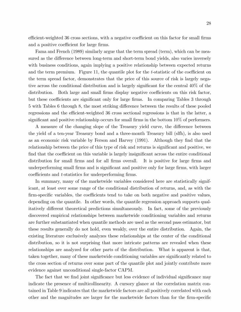
28

efficient-weighted 36 cross sections, with a negative coefficient on this factor for small firms

and a positive coefficient for large firms.

Fama and French (1989) similarly argue that the term spread (term), which can be mea-

sured as the difference between long-term and short-term bond yields, also varies inversely

with business conditions, again implying a positive relationship between expected returns

and the term premium. Figure 11, the quantile plot for the t-statistic of the coefficient on

the term spread factor, demonstrates that the price of this source of risk is largely nega-

tive across the conditional distribution and is largely significant for the central 40% of the

distribution. Both large and small firms display negative coefficients on this risk factor,

but these coefficients are significant only for large firms. In comparing Tables 3 through

5 with Tables 6 through 8, the most striking difference between the results of these pooled

regressions and the efficient-weighted 36 cross sectional regressions is that in the latter, a

significant and positive relationship occurs for small firms in the bottom 10% of performers.

A measure of the changing slope of the Treasury yield curve, the difference between

the yield of a ten-year Treasury bond and a three-month Treasury bill (slfh), is also used

as an economic risk variable by Ferson and Harvey (1991). Although they find that the

relationship between the price of this type of risk and returns is significant and positive, we

find that the coefficient on this variable is largely insignificant across the entire conditional

distribution for small firms and for all firms overall. It is positive for large firms and

underperforming small firms and is significant and positive only for large firms, with larger

coefficients and t-statistics for underperforming firms.

In summary, many of the marketwide variables considered here are statistically signif-

icant, at least over some range of the conditional distribution of returns, and, as with the

firm-specific variables, the coefficients tend to take on both negative and positive values,

depending on the quantile. In other words, the quantile regression approach supports qual-

itatively different theoretical predictions simultaneously. In fact, some of the previously

discovered empirical relationships between marketwide conditioning variables and returns

are further substantiated when quantile methods are used as the second pass estimator, but

these results generally do not hold, even weakly, over the entire distribution. Again, the

existing literature exclusively analyzes these relationships at the center of the conditional

distribution, so it is not surprising that more intricate patterns are revealed when these

relationships are analyzed for other parts of the distribution. What is apparent is that,

taken together, many of these marketwide conditioning variables are significantly related to

the cross section of returns over some part of the quantile plot and jointly contribute more

evidence against unconditional single-factor CAPM.

The fact that we find joint significance but less evidence of individual significance may

indicate the presence of multicollinearity. A cursory glance at the correlation matrix con-

tained in Table 9 indicates that the marketwide factors are all positively correlated with each

other and the magnitudes are larger for the marketwide factors than for the firm-specific

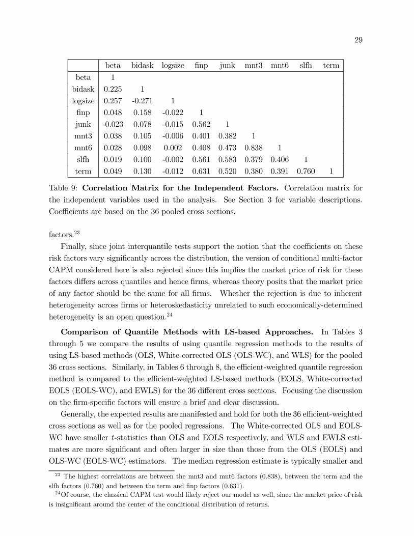
29

beta bidask logsize finp junk mnt3 mnt6 slfh term

beta 1

bidask 0.225 1

logsize 0.257 -0.271 1

finp 0.048 0.158 -0.022 1

junk -0.023 0.078 -0.015 0.562 1

mnt3 0.038 0.105 -0.006 0.401 0.382 1

mnt6 0.028 0.098 0.002 0.408 0.473 0.838 1

slfh 0.019 0.100 -0.002 0.561 0.583 0.379 0.406 1

term 0.049 0.130 -0.012 0.631 0.520 0.380 0.391 0.760 1

Table 9: Correlation Matrix for the Independent Factors. Correlation matrix forthe independent variables used in the analysis. See Section 3 for variable descriptions.

Coefficients are based on the 36 pooled cross sections.

factors.23

Finally, since joint interquantile tests support the notion that the coefficients on these

risk factors vary significantly across the distribution, the version of conditional multi-factor

CAPM considered here is also rejected since this implies the market price of risk for these

factors differs across quantiles and hence firms, whereas theory posits that the market price

of any factor should be the same for all firms. Whether the rejection is due to inherent

heterogeneity across firms or heteroskedasticity unrelated to such economically-determined

heterogeneity is an open question.24

Comparison of Quantile Methods with LS-based Approaches. In Tables 3

through 5 we compare the results of using quantile regression methods to the results of

using LS-based methods (OLS, White-corrected OLS (OLS-WC), and WLS) for the pooled

36 cross sections. Similarly, in Tables 6 through 8, the efficient-weighted quantile regression

method is compared to the efficient-weighted LS-based methods (EOLS, White-corrected

EOLS (EOLS-WC), and EWLS) for the 36 different cross sections. Focusing the discussion

on the firm-specific factors will ensure a brief and clear discussion.

Generally, the expected results are manifested and hold for both the 36 efficient-weighted

cross sections as well as for the pooled regressions. The White-corrected OLS and EOLS-

WC have smaller t-statistics than OLS and EOLS respectively, and WLS and EWLS esti-

mates are more significant and often larger in size than those from the OLS (EOLS) and

OLS-WC (EOLS-WC) estimators. The median regression estimate is typically smaller and

23 The highest correlations are between the mnt3 and mnt6 factors (0.838), between the term and theslfh factors (0.760) and between the term and finp factors (0.631).24Of course, the classical CAPM test would likely reject our model as well, since the market price of risk

is insignificant around the center of the conditional distribution of returns.

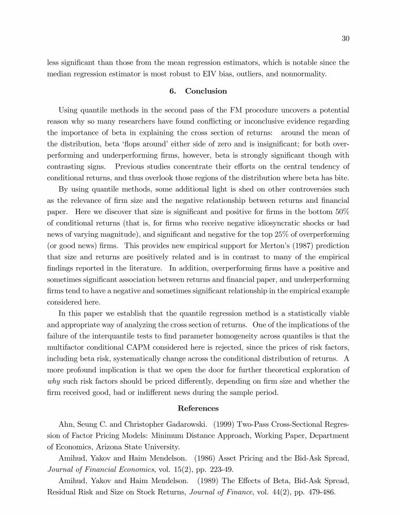
30

less significant than those from the mean regression estimators, which is notable since the

median regression estimator is most robust to EIV bias, outliers, and nonnormality.

6. Conclusion

Using quantile methods in the second pass of the FM procedure uncovers a potential

reason why so many researchers have found conflicting or inconclusive evidence regarding

the importance of beta in explaining the cross section of returns: around the mean of

the distribution, beta ‘flops around’ either side of zero and is insignificant; for both over-

performing and underperforming firms, however, beta is strongly significant though with

contrasting signs. Previous studies concentrate their efforts on the central tendency of

conditional returns, and thus overlook those regions of the distribution where beta has bite.

By using quantile methods, some additional light is shed on other controversies such

as the relevance of firm size and the negative relationship between returns and financial

paper. Here we discover that size is significant and positive for firms in the bottom 50%

of conditional returns (that is, for firms who receive negative idiosyncratic shocks or bad

news of varying magnitude), and significant and negative for the top 25% of overperforming

(or good news) firms. This provides new empirical support for Merton’s (1987) prediction

that size and returns are positively related and is in contrast to many of the empirical

findings reported in the literature. In addition, overperforming firms have a positive and

sometimes significant association between returns and financial paper, and underperforming

firms tend to have a negative and sometimes significant relationship in the empirical example

considered here.

In this paper we establish that the quantile regression method is a statistically viable

and appropriate way of analyzing the cross section of returns. One of the implications of the

failure of the interquantile tests to find parameter homogeneity across quantiles is that the

multifactor conditional CAPM considered here is rejected, since the prices of risk factors,

including beta risk, systematically change across the conditional distribution of returns. A

more profound implication is that we open the door for further theoretical exploration of

why such risk factors should be priced differently, depending on firm size and whether the

firm received good, bad or indifferent news during the sample period.

References

Ahn, Seung C. and Christopher Gadarowski. (1999) Two-Pass Cross-Sectional Regres-

sion of Factor Pricing Models: Minimum Distance Approach, Working Paper, Department

of Economics, Arizona State University.

Amihud, Yakov and Haim Mendelson. (1986) Asset Pricing and the Bid-Ask Spread,

Journal of Financial Economics, vol. 15(2), pp. 223-49.

Amihud, Yakov and Haim Mendelson. (1989) The Effects of Beta, Bid-Ask Spread,

Residual Risk and Size on Stock Returns, Journal of Finance, vol. 44(2), pp. 479-486.

31

Banz, Rolf W. (1981) The Relationship between Return and Market Value of Common

Stocks, Journal of Financial Economics, vol. 9(1), pp. 3-18.

Berk, Jonathan B. (1995) A Critique of Size-Related Anomalies, Review of Financial

Studies, vol. 8(2), pp.275-286.

Bhandari, Laxmi Chand. (1988) Debt/Equity Ratio and Expected Common Stock

Returns: Empirical Evidence, Journal of Finance, vol. 43(2), pp. 507-28.

Black, Fischer. (1972) Capital Market Equilibrium with Restrictive Borrowing, Journal

of Business, vol. 45(3), pp. 444-55.

Blume, Marshall. E. (1970) Portfolio Theory: A Step toward Its Practical Application,

Journal of Business, vol. 43(2), pp. 152-73.

Breen, William, Glosten Lawrence R., and Ravi Jagannathan. (1989) Economic Sig-

nificance of Predictable Variations in Stock Index Returns, Journal of Finance, vol. 44(5),

pp. 1177-1189.

Buchinsky, Moshe. (1995) Estimating the Asymptotic Covariance Matrix for Quantile

Regression Models: A Monte Carlo Study, Journal of Econometrics, vol. 68(2), pp. 303-38.

Buchinsky, Moshe and Jennifer Hunt. (1996) Wage Mobility in the United States,

National Bureau of Economic Research Working Paper No. 5455.

Buchinsky, Moshe and Phillip Leslie. (1997) Educational Attainment and the Chang-

ing US Wage Structure: Some Dynamic Implications, Brown University, Department of

Economics Working Paper.

Buchinsky, Moshe. (1998) Recent Advances in Quantile Regression Models: A Practical

Guideline for Empirical Research, Journal of Human Resources, vol. 33(1), pp. 88-126.

Campbell, John Y. (1987) Stock Returns and the Term Structure, Journal of Financial

Economics, vol. 18(2), pp. 373-99.

Campbell, John Y., Lettau, Martin, Malkiel, Burton G., and Yexiao Xu. (2001) Have

Individual Stocks Become More Volatile? An Empirical Exploration of Idiosyncratic Risk,

Journal of Finance, vol. 56(1), pp. 1-43.

Chan, Louis K. C., Hamao, Yasushi and Joseph Lakonishok. (1991) Fundamentals and

Stock Returns in Japan, Journal of Finance, vol. 46(5), pp. 1739-64.

Chen, Hsiu-lang and Gilbert Bassett. (2002) Attribution in the Fama-French 3-Factor

Model, Working Paper, Department of Finance, University of Illinois at Chicago.

Eide, Eric and Mark H. Showalter. (1998) The Effect of School Quality on Student

Performance: A Quantile Regression Approach, Economic Letters, vol. 58(3), pp. 345-50.

Eide, Eric and Mark H. Showalter. (1999) Factors Affecting the Transmission of Earn-

ings Across Generations: A Quantile Regression Approach, Journal of Human Resources,

vol. 34(2), pp. 253-67.

Engle, Robert F. and Simone Manganelli. (1999) CAViaR: Conditional Value at Risk

by Quantile Regression, National Bureau of Economic Research Working Paper No. 7341.

32

Engsted, Tom. (1998) Evaluating the Consumption-Capital Asset Pricing Model Using

Hansen-Jagannathan Bounds: Evidence from the UK, International Journal of Finance and

Economics, vol. 3(4), pp. 291-302.

Fama, Eugene F. and Kenneth R. French. (1989) Business Conditions and Expected

Returns on Stocks and Bonds, Journal of Financial Economics, vol. 25(1), pp. 23-49.

Fama, Eugene F. and Kenneth R. French. (1992) The Cross-Section of Expected Stock

Returns, Journal of Finance, vol. 47(2), pp. 427-65.

Fama, Eugene F. and James D. MacBeth. (1973) Risk, Return, and Equilibrium: Em-

pirical Tests, Journal of Political Economy, vol. 81(3), pp. 607-36.

Fama, Eugene F. and William Schwert. (1977) Asset Returns and Inflation, Journal of

Financial Economics, vol. 5(2), pp. 115-46.

Ferson, Wayne E. and Campbell R. Harvey. (1991) The Variation of Economic Risk

Premiums, Journal of Political Economy, vol. 99(2), pp. 385-415.

Ferson, Wayne E. and Campbell R. Harvey. (1999) Conditioning Variables and the

Cross Section of Stock Returns, Journal of Finance, vol. 54(4), pp. 1325-60.

Gibbons, Michael R. (1982) Multivariate Tests of Financial Models: A New Approach,

Journal of Financial Economics, vol. 10(1), pp. 3-27.

Gibbons, Michael R., Ross, Stephen. A., and Jay Shanken. (1989) A Test of the

Efficiency of A Given Portfolio, Econometrica, vol. 57(5), 1121-52.

Goyal, Amit, and Pedro Santa-Clara. (2002) Idiosyncratic Risk Matters!, Working

Paper, Anderson Graduate School of Management, University of California at Los Angeles.

Hansen, Lars Peter and Ravi Jagannathan. (1991) Implications of Security Market

Data for Models of Dynamic Economies, Journal of Political Economy, vol. 99(2), pp.

225-62.

Harvey, Campbell. R. (1989) Time-Varying Conditional Covariances in Tests of Asset

Pricing Models, Journal of Financial Economics, vol. 24(2), pp. 289-317.

Jagannathan, Ravi, and Zhenyu Wang. (1996) The Conditional CAPM and the Cross-

Section of Expected Returns, Journal of Finance, vol. 51(1), pp. 3-53.

Jagannathan, Ravi and Zhenyu Wang. (1998) An Asymptotic Theory for Estimating

Beta-Pricing Models Using Cross-Sectional Regression, Journal of Finance, vol. 53(4), pp.

1285-1309.

Koenker, Roger W. (2000) Galton, Edgeworth, Frisch, and Prospects for Quantile

Regression in Econometrics, Journal of Econometrics, vol. 95(2), pp. 347-74.

Koenker, Roger W. and Gilbert Basset Jr. (1978) Regression Quantiles, Econometrica,

vol. 46(1), pp. 33-50.

Koenker, Roger W. and Gilbert Basset Jr. (1982) Robust Tests for Heteroscedasticity

Based on Regression Quantiles, Econometrica, vol. 50(1), pp. 43-61.

Koenker, Roger W. and Kevin F. Hallock. (2001) Quantile Regression, Journal of

Economic Perspectives, vol. 15(4), pp. 143-56.

33

Koenker, Roger W. and Jose A. F. Machado. (1999) Goodness of Fit and Related

Inference Processes for Quantile Regression, Journal of the American Statistical Association,

vol. 94(448), pp. 1296-1310.

Kothari, S. P., Shanken, Jay and Richard G. Sloan. (1995) Another Look at the Cross-

Section of Expected Stock Returns, Journal of Finance, vol. 50(1), pp. 185-224.

Lintner, John. (1965) The Valuation of Risk Asset and the Selection of Risky Invest-

ments in Stock Portfolios and Capital Budgets, Review of Economics and Statistics, vol.

47(1), pp. 13-37.

Litzenberger, Robert. H., and Krishna Ramaswamy. (1979) The Effect of Personal

Taxes and Dividends on Capital Asset Prices: Theory and Empirical Evidence, Journal of

Financial Economics, vol. 7(2), pp. 163-96.

Merton, Robert C. (1987) A Simple Model of Capital Market Equilibrium with Incom-

plete Information, Journal of Finance, vol. 42(3), pp. 483-510.

MacKinlay, A. Craig and Matthew P. Richardson. (1991) Using Generalized Method

of Moments to Test Mean-Variance Efficiency, Journal of Finance, vol. 46(2), pp. 511-27.

Morillo, Daniel S. (2000) Monte Carlo American Option Pricing with Nonparametric

Regression, in: Essays in Nonparametric Econometrics, Dissertation, University of Illinois.

Mossin, Jan. (1966) Equilibrium in a Capital Asset Market, Econometrica, vol. 34(4),

pp. 768-83.

Shanken, Jay. (1992) On the Estimation of Beta Pricing Models, Review of Financial

Studies, vol. 5(1), pp. 1-33.

Sharpe, William. (1964) Capital Asset Prices: A Theory of Market Equilibrium Under

Conditions of Risk, Journal of Finance, vol. 19(3), pp. 425-42.

White, Halbert. (1980) A Heteroskedasticity-Consistent Covariance Matrix Estimator

and a Direct Test for Heteroskedasticity, Econometrica, vol. 48(4), pp. 817-38.

34

Appendix 1Data Descriptions

Firm-Specific Data (Source is Center for Research in Security Prices - CRSP)Bidlo: The lowest sale or closing bid on the day.

Askhi: The highest sale or closing ask on the day.

Price: The closing price or the negative bid/ask average on the day.

Return: The change in the total value of an investment in a common stock over some

period of time per dollar of initial investment. It is the holding period return for a sale on

that day. It is based on a purchase on the most recent time previous to the current day

when the security had a valid price (usually the day before).

Marketwide Data (Sources are CRSP and the Federal Reserve’s Board ofGovernors’ web page)Market: The return on the value-weighted market portfolio, constructed by CRSP.

finp: Financial paper. The proxy for the risk-free rate, defined as directly placed,

unsecured, short-term negotiable promissory notes. The yield is the unweighted average of

offering rates reported each business day to the Federal Reserve Bank of New York.

junk: The yield on Moody’s Baa-rated corporate bonds less the yield on Aaa-rated

corporate bonds. Aaa and Baa types of yield are defined as average yield to maturity on

selected long-term bonds.

slfh: Ten-year constant maturity T-bond yield less the three-month constant maturity

T-bill rate.

term: The spread between a ten-year and a one-year T-bond yield, ten-year yield minus

one-year yield. Constant maturity yields on Treasury securities at constant, fixed maturity

are constructed by the Treasury Department, based on the most actively traded marketable

Treasury securities. Yields on these issues are based on composite quotes reported by U.S.

government securities dealers to the Federal Reserve Bank of New York. To obtain the

constant maturity yields, personnel at Treasury construct a yield curve each business day

and yield values are then read from the curve at fixed maturities.

mnt6: Six-month Treasury constant maturity yield less the one month yield (finp).

Yields on Treasury securities at constant, fixed maturity are constructed by the Treasury

Department, based on the most actively traded marketable Treasury securities. Yields on

these issues are based on composite quotes reported by U.S. government securities dealers

to the Federal Reserve Bank of New York.

mnt3: Same as above, three-month yield less the one-month yield.

Dummy Variables for Calendar and Trading EffectsDummy variables: DV1-4 are dummies for Tuesday through Friday; DV5 is the square

root of the gap between trading days; DV6-14 are dummies for months March through

November; and DV15-22 are dummies for weeks of the month for December and January.