Embed Size (px)
Citation preview
A Quantitative Analysis of the Cairclip O3/NO2 Sensor
by
Brenda Lee Reid
A thesis submitted in partial fulfillment of the requirements for the degree of
Master of Science
in
Environmental Health Sciences
Department of Public Health Sciences
University of Alberta
© Brenda Lee Reid, 2015
ii
ABSTRACT
Ozone (O3) and nitrogen dioxide (NO2) are two criteria pollutants that can
result in adverse outcomes that effect both natural environments and human
health. As these outcomes have a significant impact on people and their
environments, it is necessary to closely monitor the levels of these gases in the
ambient air. Currently, air quality monitoring in Edmonton is reported through the
Air Quality Health Index (AQHI) as determined from measurements acquired
from the four centralized ambient monitoring stations across the city. While the
air quality data collected at the centralized monitoring stations provides the public
with a generalized idea of the air quality for the day, they are unable to measure
real time concentrations of near-field sources of pollutants based on an
individual’s daily activity patterns. These unique activity patterns are specific to
an individual and differ from one person to the next.
The Cairclip sensor is representative of new technology in personal exposure
monitors as they are small, lightweight and highly portable. In order to gain
further understanding in the operational capacities and limitations of these
sensors, the Cairclip O3 + NO2 sensor was tested in a two phase study. In phase
one, the Cairclip was deployed at the Edmonton south monitoring station in order
to determine their accuracy against the centralized monitor, as well as the level of
precision between paired sensors. In phase two, the sensors were tested in various
scenarios measuring near-field concentration exposures of O3 + NO2 at the
personal level as well as at the subject’s residence.

iii
The findings of phase one precision resulted in a percent relative deviation
(%RSD) for one hour averaged concentrations with outliers removed that ranged
from +/-20% to +/-11%. Phase one accuracy was calculated using mean absolute
percent difference (MAPD) for data sets screened for outliers and based on one
hour averaged concentrations of O3 + NO2, these values ranged from +/-40% to
+/-29%, respectively. In phase two, the Cairclips responded in a highly varied
pattern when challenged during personal exposure monitoring in various settings
where pollutant concentrations originated from near field sources.
In conclusion, phase one determined that the level of accuracy of the Cairclips
in contrast to the Edmonton south centralized station was poor. Personal exposure
monitoring in various scenarios in phase two showed that the most significant
findings were found in environments that are in close proximity to vehicular
traffic and where sources of O3 and NO2 are prevalent due to gas-fired appliances.
The specific settings were determined by the data collected in restaurants located
close to high volumes of traffic and on public transit routes.
Prior to use in further research, it is recommended that the accuracy and
precision of the sensors be retested. In addition, further research in air monitoring
of levels O3 and NO2 in closed, built environments and on various public
transportation routes using the Cairclip may be warranted.

iv
ACKNOWLEDGEMENTS
A special note of sincere gratitude is extended to Dr. Warren Kindzierski,
Professor/Advisor, who has provided his expansive expertise and knowledge in
the field of air quality research. Dr. Kindzierski’s support and guidance reached
beyond the research project and were fundamental to the successful completion of
this Masters of Environmental Health program.
Thank you to my mother and father, Robert and Doreen, who taught me the
value of hard work and the beauty of kindness. In addition, a heartfelt thank you
to Jesus Serrano Lomelin (PhD student), Maryanne Reavie (MEd), Margaret Eggo
(PhD), Jeff Hehn (Engineer), Robin Baillie (Engineer), Neil Greening (Graphics
Artist), Debra Marshall (photographer), Aynul Bari, Xioming Wang, Yutaka
Yasui (Professor), Gian Jhangri (Professor), Shelley Morris (Alberta
Environment) and Dr. Claude Prefontaine. Finally, I wish to extend a sincere and
heartfelt thank you to all my friends and family for their support and love.

v
TABLE OF CONTENTS
ABSTRACT II
ACKNOWLEDGEMENTS IV
LIST OF TABLES XI
LIST OF FIGURES XIII
LIST OF EQUATIONS XVII
LIST OF SYMBOLS, ABBREVIATIONS AND ACRONYMS XVIII
1 INTRODUCTION 1
1.1 Objective of Study 3
1.2 Problem Statement 4
1.3 Hypothesis 4
2 BACKGROUND 5
2.1 Environmental Pollutants of Interest 5
2.1.1 Nitrogen Dioxide 6
2.1.2 Ozone 10
2.2 Global, National and Local Standards for Air Quality 12

vi
2.2.1 Global 12
2.2.2 National Standards: United States 16
2.2.3 National Standards: Canada 17
2.2.4 Local Standards: Alberta and Edmonton 20
2.3 Human Exposures to Pollutants 22
2.3.1 Exposure Science 25
2.3.2 Source Based and Receptor Based Exposure 26
2.3.3 Direct Versus Indirect Approach to Measuring Human Exposure 29
2.4 Types of Air Monitoring Methods 31
2.4.1 Station Monitoring Versus Personal Monitoring 34
2.4.2 Passive Monitors 38
2.4.3 Active Monitors 41
2.4.4 Personal Monitors 44
2.5 Components of Personal Exposure Monitoring 49
2.5.1 Real Time Monitoring and Time Activity Diaries 50
2.5.2 Microenvironments 51
2.6 Summary 52
3 METHODOLOGY 54
3.1 Basis of Study 54
3.2 Description of Monitors 55

vii
3.3 Phase One: Purpose and Design 57
3.3.1 Location and Deployment of Cairclip Sensors for Phase One 58
3.3.2 Time of Day and Duration of Data Collection for Phase One 63
3.3.3 Quality Control and Quality Assurance Experiments 63
3.3.4 Determining Field Precision: Cairclip to Cairclip 64
3.3.5 Determining Field Accuracy: Cairclips to NAPS Station Monitor 65
3.3.6 Data Selection Criteria 66
3.3.7 Datasets Group One, Two and Three for Comparison 67
3.4 Phase Two: Purpose and Design 68
3.5 Indoor and Outdoor Residential Monitoring 71
3.6 Personal Exposure Monitoring 73
3.6.1 Outdoor Monitoring at Jasper Avenue and 109th Street 75
3.6.2 Outdoor Monitoring at 97th Avenue and 109th Street 76
3.6.3 Outdoor Monitoring of Whyte Avenue to 109th Street 76
3.6.4 Outdoor Monitoring of 99th Street to Whyte Avenue 77
3.7 Commuter Monitoring On Public Transportation 78
3.8 Indoor Monitoring at High Volume Traffic Areas 79
3.8.1 Indoor Monitoring at 109th Street and 88th Avenue 80
3.8.2 Indoor Monitoring at 99th Street and 89th Avenue 81
3.8.3 Indoor Monitoring at 104th Avenue and Whyte Avenue 82

viii
4 RESULTS AND DISCUSSION 84
4.1 Phase One Replicate Monitoring and Field Precision of Cairclips 84
4.1.1 Precision Results Cairclip 1 to Cairclip 2 85
4.1.2 Precision Results Cairclip 1 to Cairclip 3 88
4.1.3 Precision Results Cairclip 1 to Cairclip 4 90
4.1.4 Precision Results Cairclip 2 to Cairclip 3 92
4.1.5 Precision Results Cairclip 2 to Cairclip 4 94
4.1.6 Precision Results Cairclip 3 to Cairclip 4 96
4.2 Monitoring at Edmonton South Station and Field Accuracy 98
4.2.1 Accuracy Results Cairclip 1 to Station Monitor 101
4.2.2 Accuracy Results Cairclip 2 to Station Monitor 103
4.2.3 Accuracy Results for Cairclip 3 to Station Monitor 105
4.2.4 Accuracy Results for Cairclip 4 to Station Monitor 107
4.3 Phase Two: Indoor and Outdoor Residential Monitoring 110
4.4 Phase Two: Personal Exposure Monitoring 114
4.5 Monitoring of Busy Intersections and Roadways 115
4.5.1 Outdoor Monitoring of Jasper Avenue at 109th Street 117
4.5.2 Outdoor Monitoring at 97th Avenue and 109th Street 119
4.5.3 Outdoor Monitoring of Whyte Avenue to 109th Street 123
4.5.4 Outdoor Monitoring at 99th Street to Whyte Avenue 125
ix
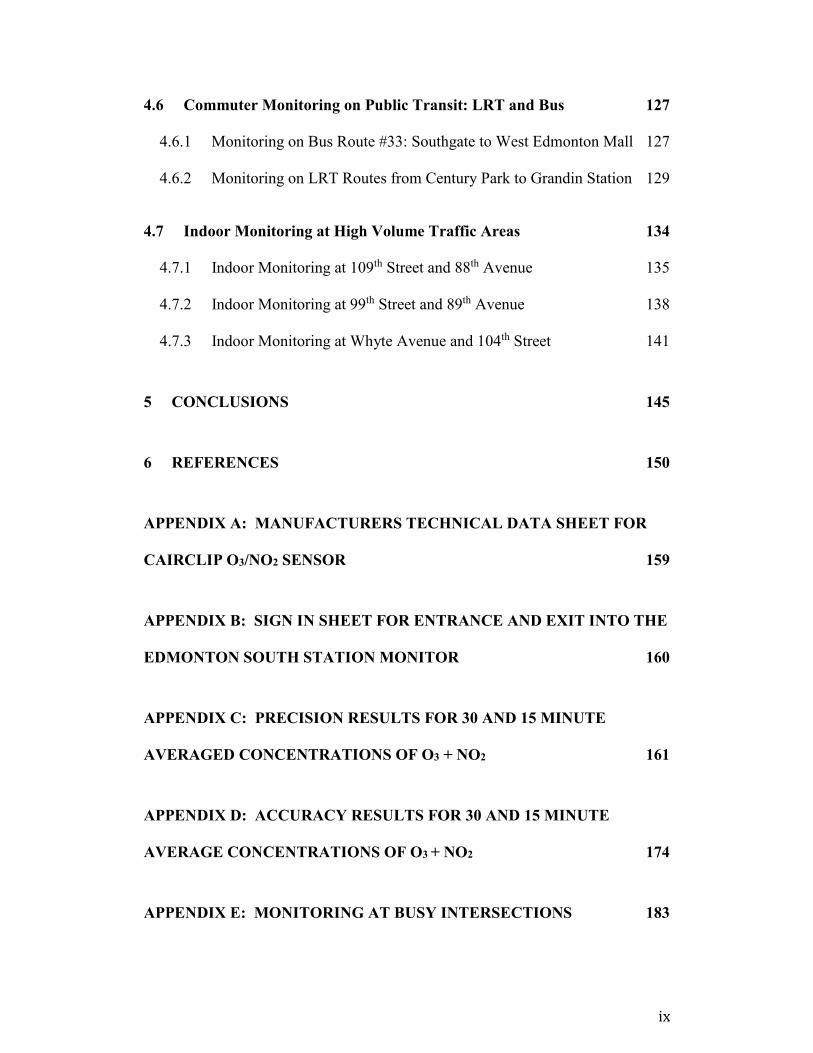
4.6 Commuter Monitoring on Public Transit: LRT and Bus 127
4.6.1 Monitoring on Bus Route #33: Southgate to West Edmonton Mall 127
4.6.2 Monitoring on LRT Routes from Century Park to Grandin Station 129
4.7 Indoor Monitoring at High Volume Traffic Areas 134
4.7.1 Indoor Monitoring at 109th Street and 88th Avenue 135
4.7.2 Indoor Monitoring at 99th Street and 89th Avenue 138
4.7.3 Indoor Monitoring at Whyte Avenue and 104th Street 141
5 CONCLUSIONS 145
6 REFERENCES 150
APPENDIX A: MANUFACTURERS TECHNICAL DATA SHEET FOR
CAIRCLIP O3/NO2 SENSOR 159
APPENDIX B: SIGN IN SHEET FOR ENTRANCE AND EXIT INTO THE
EDMONTON SOUTH STATION MONITOR 160
APPENDIX C: PRECISION RESULTS FOR 30 AND 15 MINUTE
AVERAGED CONCENTRATIONS OF O3 + NO2 161
APPENDIX D: ACCURACY RESULTS FOR 30 AND 15 MINUTE
AVERAGE CONCENTRATIONS OF O3 + NO2 174
APPENDIX E: MONITORING AT BUSY INTERSECTIONS 183

x
APPENDIX F: INDOOR MONITORING AT HIGH VOLUME TRAFFIC
AREAS 188

xi
LIST OF TABLES
Table 1. Global standards for O3 and NO2 16
Table 2. NAAQS of O3 and NO2 for the United States 17
Table 3. Canadian and Alberta AQG for O3 and NO2 (NOx) 20
Table 4. Field precision results of Cairclip 1 to Cairclip 2 86
Table 5. Linear regression results for field precision Cairclip 1 to
Cairclip 2 87
Table 6. Field precision results of Cairclip 1 to Cairclip 3 89
Table 7. Linear regression results for field precision of Cairclip 1 to
Cairclip 3 90
Table 8. Field precision results of Cairclip 1 to Cairclip 4 91
Table 9. Linear regression results for field precision Cairclip 1 to 4 92
Table 10. Field precision results of Cairclip 2 to Cairclip 3 93
Table 11. Linear regression results for field precision of Cairclip 2 to
Cairclip 3 94
Table 12. Field precision results of Cairclip 2 to Cairclip 4 95
Table 13. Linear regression results for field precision of Cairclip 2 to
Cairclip 4 96
Table 14. Field precision results for Cairclip 3 to Cairclip 4 97
Table 15. Linear regression results for field precision of Cairclip 3 to
Cairclip 4 98
Table 16. Field accuracy results of Cairclip 1 to station monitor 102
Table 17. Linear regression results for field accuracy of Cairclip 1 to
station monitor 103
Table 18. Field accuracy results of Cairclip 2 to station monitor 104
Table 19. Linear regression results for field accuracy of Cairclip 2 to
station monitor 105

xii
Table 20. Field accuracy results of Cairclip 3 to station monitor 106
Table 21. Linear regression results for field accuracy of Cairclip 3 to
station monitor 107
Table 22. Field accuracy results of Cairclip 4 to station monitor 108
Table 23. Linear regression results for field accuracy of Cairclip 4 to
station monitor 109
Table 24. Descriptive statistics of concentration ratios Cairclip 2 to
Cairclip 3 112

xiii
LIST OF FIGURES
Figure 1. Diagram of potential household pollutants and their sources 28
Figure 2. Diagram of a passive sampler 39
Figure 3. Diagram of a Cairclip O3/NO2 monitor 42
Figure 4. Example of the Cairclip sensor O3/NO2 used in the study 57
Figure 5. The location of the Edmonton south monitoring station 59
Figure 6. Photograph of the Edmonton south station monitor 59
Figure 7. Hardware used to secure the shelter for the Cairclips 60
Figure 8. Set-up of the shelter at the station monitor 61
Figure 9. Cairclip sensors secured under the shelter at the station monitor 62
Figure 10. The shelter set-up in relation to the air intake of the
station monitor 62
Figure 11. Map of approximate location of monitoring sites in phase two 70
Figure 12. Photograph showing the indoor residential placement of the
Cairclip 72
Figure 13. Photograph of outdoor residential placement of Cairclip 72
Figure 14. Photograph of Cairclip attached under shelter in backyard setting 73
Figure 15. Photograph of Cairclip placement for personal monitoring 74
Figure 16. Photograph of Cairclip attached to upper arm with warnings
displayed 75
Figure 17. Diagram of the Jasper Ave./109th St. & 97th Ave./109th St.
monitoring locations 76
Figure 18. Diagram of the 99th St./Whyte Ave & Whyte Ave./109th St.
monitoring locations 77
Figure 19. Map of bus and LRT routes monitored 79
Figure 20. Diagram of the 109th St. & 88th Ave. indoor monitoring site 81
xiv
Figure 21. Diagram of the 99th St. & 89th Ave. monitoring site 82
Figure 22. Diagram of the 104th St. & Whyte Ave. indoor monitoring site 83
Figure 23. Graph comparing precision data of Cairclip 1 to Cairclip2 87
Figure 24. Graph comparing precision data of Cairclip 1 to Cairclip 3 90
Figure 25. Graph comparing precision data of Cairclip 1 to Cairclip 4 92
Figure 26. Graph comparing precision data of Cairclip 2 to Cairclip 3 94
Figure 27. Graph comparing precision of Cairclip 2 to Cairclip 4 96
Figure 28. Graph comparing precision of Cairclip 3 to Cairclip 4 98
Figure 29. Comparison of accuracy results of Cairclips to station monitor 101
Figure 30. Graph of accuracy results of Cairclip 1 to the station monitor 103
Figure 31. Graph of accuracy results of Cairclip 2 to the station monitor 105
Figure 32. Graph of accuracy results of Cairclip 3 to station monitor 107
Figure 33. Graph of accuracy results Cairclip 4 to station monitor 109
Figure 34. Map showing approximate location of residential monitoring 111
Figure 35. Graph of mean ratio results of indoor (CC2) vs outdoor (CC3)
concentrations 112
Figure 36. Map showing the urban site outdoor sites used for personal
exposure monitoring 116
Figure 37. Comparison of Cairclip to station monitor on
Sept. 13, 2013 at Jasper Ave. & 109th St. 118
Figure 38. Comparison of Cairclip to station monitor on
Sept. 27, 2013 at Jasper Ave. & 109th St. 118
Figure 39. Graph of comparison of Cairclip to station monitor on
Oct. 10, 2013 at 97th Ave. and 109th St. 121
Figure 40. Graph of comparison of Cairclip to station monitor on
Oct. 11, 2013 at 97th Ave. and 109th St. 121

xv
Figure 41. Graph of comparison of Cairclip to station monitor on
Jan 9, 2014 at 97th Ave. and 109th St. 122
Figure 42. Graph of comparison of Cairclip to station monitor on
Nov. 29, 2013 at Whyte Ave. & 109th St. 124
Figure 43. Graph of comparison of Cairclip to station monitor on
Dec. 23, 2013 at Whyte Ave. & 109th St. 124
Figure 44. Graph of comparison of Cairclip to station monitor on
Dec. 15, 2013 at 99th St. & Whyte Ave. 126
Figure 45. Graph of comparison of Cairclip to station monitor on bus route
#33 on Oct. 22, 2013 129
Figure 46. Graph comparing Cairclip to station monitor on LRT on
Sept. 16, 2013 131
Figure 47. Graph of comparison of Cairclip to station monitor on LRT on
Oct. 10, 2013 131
Figure 48. Graph of comparison of Cairclip to station monitor on LRT on
Oct. 11, 2013 132
Figure 49. Graph of comparison of Cairclip to station monitor on LRT on
Oct. 15, 2013 132
Figure 50. Graph of comparison of Cairclip to station monitor on LRT on
Oct. 22, 2013 133
Figure 51. Map of indoor monitoring sites 135
Figure 52. Graph of comparison of Cairclip to station monitor on
Nov. 28, 2013 at 109th St. & 88th Ave. 136
Figure 53. Graph of comparison of Cairclip to station monitor on
Nov. 28, 2013 at 109th St. & 88th Ave. 137
Figure 54. Graph of comparison of Cairclip to station monitor on
Nov. 28, 2013 at 109th St. & 88th Ave. 137
Figure 55. Graph of comparison of Cairclip to station monitor on
Dec. 2, 2013 at 99th St. & 89th Ave. 139
Figure 56. Graph of comparison of Cairclip to station monitor on
Dec. 10, 2013 at 99th St. & 89th Ave. 139

xvi
Figure 57. Graph of comparison of Cairclip to station monitor on
Dec. 12, 2013 at 99th St. & 89th Ave. 140
Figure 58. Graph of comparison of Cairclip to station monitor on
Dec. 17, 2013 at 99th St & 89th Ave. 141
Figure 59. Graph of comparison of Cairclip to station monitor on
Jan. 9, 2014 at 104th St. & Whyte Ave. 143
Figure 60. Graph of comparison of Cairclip to station monitor on
Jan. 10, 2014 at 104th St. & Whyte Ave. 143

xvii
LIST OF EQUATIONS
Equation 1: Percent Relative Standard Deviation (%RSD)…………………….62
Equation 2: Standard Deviation (SD)…………………………………..............62
Equation 3: Mean Absolute Percent Difference (MAPD)………………...........63

xviii
LIST OF SYMBOLS, ABBREVIATIONS AND ACRONYMS
AAADMS Alberta ambient air data management
AQG Air Quality Guide
AQHI Air Quality Health Index
AQI Air Quality Index
AWMA Air and Waste Management Association
CAAQS Canadian Ambient Air quality Standards
CASA Clean Air Strategic Alliance
CC Cairclip
CO Carbon monoxide
CO2 Carbon dioxide
DPAS Directional passive air sampler
DQO Data Quality Objective
ECHA Edmonton Clinic Health Academy
ECSM Edmonton central station monitor
EPHT Environmental Public Tracking
FCAA Federal clean air act
H2S Hydrogen Sulfide
HAPS Hazardous air pollutants
HC Hydrocarbons
HDDM- Highorder Decoupled Direct Method-Community Multiscale Air
CMAQ Quality
JRC Joint Research Center
LOD Level of detection
LV Limit values
MAL Maximum accepted level
MAPD Mean absolute percent difference
MDL Maximum desirable level
MTL Maximum tolerated level
NAAQS National Ambient Air quality Standards
NAPS National Air Pollution Surveillance

xix
NH3 Ammonia
NO Nitrogen oxide
NO2 Nitrogen dioxide
NOx Total concentration of NO and NO2
NRC National Research Council
O3 Ozone
PEM Personal exposure monitoring
PPB Parts per billion
PSD Prevention of significant deterioration
S-R Source-receptor relationship
SD Standard deviation
SGS Southgate Station
SO2 Sulfur dioxide
SO2 Sulfur dioxide
TAD Time activity diary
Ug/mg3 Micrograms per cubic meter
US EPA United States Environmental Protection Agency
UV Ultraviolet
VOC Volatile organic compounds
WEM West Edmonton Mall
WHO World Health Organization

1
1 INTRODUCTION
The term environmental health encompasses a range of external factors, which
may directly or indirectly affect an individual or an identified source population.
These extrinsic factors may be biological, chemical or physical in nature and all
have the potential to affect the health and well-being of all living organisms both
positively and negatively.
Ambient air pollution may be defined as a combination of gases that are
constantly present within an environment whether urban, suburban or rural. Often
these gases are man-made through industrial, agricultural and commuting
practices. Subsequently, potential exposures exist due to the activities of people in
their homes and the household products used, which often contribute to
concentrations of pollutants in a built environment where people spend significant
amounts of time.
With this in mind, air quality plays a significant role in both human and
environmental health. In a world experiencing continued, exponential growth in
population and industrial activities, air pollution has the potential to be an ever-
increasing environmental and human health issue. In order to address the human
and environmental impact associated with air pollution, it is important to define
which are the “criteria air pollutants” of concern; through what activities are they
formed; how these pollutants interact with others in an environment; and what are
the potential byproducts of theses interactions. Importantly, this information aims
to provide an understanding of the intricate interaction between living organisms

2
in both built and ambient environments to air pollutants in order to set standards
and promote optimal health.
In order to facilitate knowledge for science, policy and public purposes we
must gain a more in-depth understanding of the degree of human health effects
associated with exposure to air pollution based on duration, location and
concentration of exposure. Personal exposure monitors may have the potential not
only to provide for identification of geographically problematic areas but also to
promote an individual’s awareness to make conscientious choices and inspire a
prevention-based attitude to improving their air quality.
Lifestyle choices like taking public transportation and making conscientious
decisions when purchasing certain consumable household products can help to
reduce the negative impact on the natural environment. Improving air quality and
environmental health is not solely the responsibility of the government; people
must do their part in changing the things that we can at the individual level.
For the purposes of this study the focus is on air quality and the effects of two
specific criteria pollutants, ground level ozone (O3) and nitrogen dioxide (NO2).
These gases are commonly present in indoor and outdoor environments as a result
of anthropogenic activities, interactions with other air contaminants and certain
events of nature. The human health effects of high concentrations of these gases is
linked to respiratory ailments, particularly for vulnerable members of the
population. The advent of personal exposure monitoring devices used in
conjunction with time activity records/diaries show promise for a new paradigm
in air quality monitoring. Understanding the spatiotemporal difference between

3
ambient and personal exposure to air pollutants may be key to providing
education, improve programing and development of policy standards that act
more proactively to protect both human and environmental health.
This dissertation will provide a background discussion of the formation of O3
and NO2, the current regulatory standards, the effects they have on environmental
and human health and components of exposure science in effectively measuring
human exposure. Following the background section, details of this thesis research
using the Cairclip O3/NO2 sensor to study personal air quality will be discussed in
the methodology, results and conclusions sections, respectively.
1.1 Objective of Study
The objective of this study was to compare and test the efficacy and unique
capabilities of new technology in personal monitors, the Cairclip, in measuring
concentration exposures to O3 + NO2. This objective was achieved by measuring
the Cairclip’s level of accuracy and precision; and to assess its ability in personal
exposure monitoring. Through testing these new personal air monitoring devices
in various capacities and scenarios, this research aims to be useful in determining
if these sensors can provide valuable insight about near-field sources of pollutants
in indoor and outdoor environments that may indicate risk potential.
In the following research, the findings aim to provide insight and promote
further research into the future of air quality monitoring of pollutants in growing
urban environments where people live and interact closely with expanding
industrial operations and vehicular traffic. Importantly, it is critical for the public
to understand the effects that poor ventilation and certain human activities have

4
on the air quality within indoor environments. Finally, the research and findings
of this study aims to provide some information that may bridge the gap between
current standards of air monitoring based on ambient centralized station
monitoring and personal monitoring of air pollution.
1.2 Problem Statement
Past and current trends in studying human and environmental exposure to air
pollutants have been focused on measuring far-field concentrations at the ambient
level. In reality, science has shown that true human exposure to air pollution may
be better represented by measuring exposure to air pollutants on a near-field, real
time basis at the receptor level, known as personal exposure monitoring.
Currently, a gap in scientific knowledge exists in understanding to what degree
personal exposure monitoring differs from that of ambient fixed site monitoring.
1.3 Hypothesis
Personal exposure monitoring of near-field sources of pollution are more
representative of actual human or environmental exposure and potential risk than
that of fixed-site, centralized monitoring of far-field sources.
5
2 BACKGROUND
Air quality monitoring of enclosed spaces dates back to 1851 where workers’
exposures to concentrations of carbon dioxide (CO2), O3 and hazardous airborne
dust in coal mines were tested in order to evaluate possible adverse health
outcomes (Fenske, 2010). While in the 1970’s, the emergence of personal
monitors for measuring environmental pollutants showed promising potential in
the field of air quality, continued research and development was warranted
(Wallace, 1982). Since this time, the trend towards designing personal monitoring
devices that are accurate, precise, affordable and simple to use has been a focus
for many researchers working in the field of exposure analysis (Wallace, 1982).
Even though studies have shown that exposure to air pollution has measureable,
detrimental effects on human and environmental health, scientists have yet to
draw a direct causal link between certain specific pollutants and illness (Labelle,
1998).
2.1 Environmental Pollutants of Interest
Throughout the years, environmental monitoring of air quality has been an
important contributory factor in determining and forecasting disease patterns in
human and environmental health. The concentration of pollutants in ambient air
has been a cause of concern for many decades. Organizations such as the World
Health Organization (WHO), the United States Environmental Protection Agency
(US EPA) and Environment Canada are actively involved in monitoring and
evaluating changes in pollutant concentrations in ambient air. This information is
then used to revise air quality standards where needed to protect the both the

6
public and the natural environment (WHO, 2005a; US EPA, 2014a; Environment
Canada, 2013).
O3 and NO2 have an intricate relationship as they are both found to be
respiratory irritants. Studies have conclusively linked tropospheric O3 to
respiratory ailments, but have been somewhat inconclusive as to the degree of
health effects associated with exposure to NO2. Generally in environments, when
NO2 levels are low O3 levels will be high; and, if NO2 levels are high then
concentrations of O3 are low. NO2 is mainly formed due to anthropogenic
activities involving combustion processes, which include vehicular engines, as
well as industrial and agricultural processes. NO2 plays a critical role in the
formation of tropospheric O3 (US EPA, 2014a; Environment Canada, 2013b).
2.1.1 Nitrogen Dioxide
NO2 is one of the two most common nitrogen oxides (NOX) gases. The
chemical structure of NO2 is a nitrogen (N) atom bonded with two oxygen (O)
atoms. The chemical symbol NOx represents the combination of nitric oxide (NO)
and NO2; literature commonly refers to this when discussing nitrogen gases
(National Library of Medicine, 2013). Other elements in the NOx family of gases
are nitrous acid and nitric acid (US EPA, 2014b). NOx (NO2) are formed as by-
products of the combustion process associated to vehicular engines that burn coal,
oil and diesel fuel; industrial activities such as welding, electroplating, engraving
and dynamite blasting; and the expansion of agricultural process which has
become a major contributor to increased concentrations of NO2 in the ambient air
(Sandell, 1998; National Library of Medicine, 2013). Certain in-home activities
7
such as cigarette smoking and the use of kerosene or gas stoves may have the
potential to promote adverse human health effects due to production of high levels
of NOx in enclosed spaces (National Library of Medicine, 2013).
NOx, a colorless gas, reacts with O3 in the atmosphere where it is converted to
NO2, which is a yellowish or reddish brown colored gas (Sandell, 1998; Koehler
et al., 2013). NO2 engages in a complex chain of both chemical and
photochemical reactions with NO, O3 and other gases. Ambient air concentrations
of NO2 are generally highest in fall and winter months when weather conditions
are stable, with concentrations dissipating as the distance from source increases
(Gilbert et al., 2003; WHO, 2005a).
NOx, along with carbon monoxide (CO) and volatile organic compounds
(VOC’s) are O3 precursors. When these gases react in the presence of sunlight, the
by-product formed is tropospheric or ground level O3 (Kindzierski, et al., 2007).
The type of interaction that takes place is a photochemical reaction, which occurs
as a result of oxidation-reduction reactions induced by ultraviolet light. Ground
level O3 quickly reacts with NOx in the environment to form NO2 (National
Library of Medicine, 2013).
Future global emissions of NOx have been predicted to increase as developing
countries continue to evolve and grow in many economic sectors. Economic
development often correlates with an increase in overall standards for quality of
life. The effects of economic growth often correspond to increased ownership and
use of personal vehicles, which in-turn contributes to emission load and
degradation of air quality. This is a problem in developing countries with lax

8
governmental regulations and poor compliance of industry in adhering to air
quality standards (Bradley and Jones, 2002).
In a study conducted by Bradley and Jones (2002), the researcher evaluated
power generation and transportation technologies that produce less NOX than
conventional practices. The aim of this research was to find alternatives to
conventional technologies for power generation and transportation technologies
that produce fewer NOx emissions in developing countries. The researchers
concluded that the concept of a technology leap may be a possible solution for
developing countries to counter-balance the projected increase in NOx emission
(Bradley and Jones, 2002).
As discussed outdoor ambient production of NO2 is a source of human and
environmental exposure. This said, indoor concentrations of NO2 in built
environments has shown to be a significant source of human exposure. As
reported by the National Academy of Science (NAS) (1991), studies spanning
over several years show indoor levels of NO2 tend to be of greater concern than
outdoor levels. Concentrations of the pollutant, NO2, in built environments have
been shown to be consistently and significantly higher than that measured
outdoors. Elevated levels of indoor concentrations of NO2 are in part due to an
increase in popularity and use of gas fired cooking appliances, home heating
systems such as fireplaces and inadequate indoor ventilation or air exchange
systems (National Research Council (NRC), 1991; National Library of Medicine,
2013).

9
In Canada in 2005 the main emission sources of NOX originated from the
transportation sector, contributing 53% of the ambient air concentration
(Kindzierski, et al., 2007). The remaining contributors were upstream oil and gas
industry at 19% with various other sources accounting for 18% (Kindzierski, et al.
2007). Similar to Canada’s statistics, Alberta’s air emissions for NOX gas was
primarily attributed to upstream oil and gas operations with smaller contributions
associated to natural gas, oil sands and other industries (Kindzierski, et al., 2007).
Although the full impact of health effects associated with exposure to NO2 are
not yet certain, air quality monitoring of NO2 is important. From a human health
perspective, when exposure duration is long enough and concentration is high
enough, NO2 may have adverse effects on vulnerable populations and ecosystems
(WHO, 2003b). Exposures to concentrations of NO2, have been associated to
induce or exacerbate problems with the human respiratory system. These
respiratory responses may include a number of conditions such as bronchitis,
pneumonia and increased susceptibility to viral infections (Sandell, 1998).
Similarly, Yoshida and Kasama (1987) concluded that inhaled concentrations
of NO/NO2 had the potential to adversely react with human tissues of the
respiratory system cell membranes, contribute to peroxidation of lipids in cell
membranes, increase the risk of cancer and promote premature aging (Yoshida
and Kasama, 1987).
Day to day fluctuations of NO2 has been reported to increase risk of ischemic
stroke during summer months (Johnson et al., 2013). In a study conducted in
Edmonton, Alberta by researchers Johnson et al., (2013), the scientists measured
10
the relationship between highly spatially resolved estimates of NO2 and
emergency room visits for those people suffering strokes. Unlike short term,
fluctuating levels, medium and long-term human exposure to ambient air
pollution was found to be less likely to increase risk of stroke (Johnson et al.,
2013).
In the environment, NO2 contributes to the formation of ground level ozone, as
well as the destruction of stratospheric ozone and delicate ecosystems (USEPA,
2014b; NRC, 1991). Ambient air containing NO2 is capable of damaging and
preventing optimum plant growth. The pollutant may damage the leaves of plants,
inhibit photosynthesis and impede growth of vegetation (US EPA, 2014b). When
NO2 is deposited on land, in estuaries, lakes and streams, acidification and excess
fertilization can occur. Although the extent of harm that NO2 has on ecosystems is
not thoroughly understood, effects such as alterations in biodiversity, water
quality, mutation or extinction of fish and possibly wildlife have found to be
linked to exposure of this pollutant (US EPA, 2014b; WHO, 2000c).
2.1.2 Ozone
The chemical structure of O3 is comprised of three oxygen atoms, a
configuration that makes it extremely reactive with a potential to decompose
explosively in the environment. As a result of O3’s powerful oxidative action, the
chemical has been used in several industrial and consumer processes that are
associated with oxidation. The molecular weight of O3 is 48g mol-1 and is it is
described as a pale blue gas with a pungent odor (US EPA, 2014b).
11
O3 formation occurs in the atmosphere as a result of photochemical reactions in
the presence of sunlight as well as in the presence of precursor pollutant gases
such as NO2 and VOC’s (WHO, 2005a). O3 levels are generally highest in the
summer due to warmer temperatures and more hours of daylight resulting in
higher levels and longer duration of ultraviolet light (UV). In rare situations,
according to past findings by the US EPA (2014b), high O3 levels have been
recorded in elevated regions of the western states during fall and winter months
where temperatures were at or below the freezing point. This was attributed to the
high ambient air concentrations of VOC’s and NOx emissions in this geographical
area (US EPA, 2014b).
O3 is classified as either stratospheric or tropospheric. The stratosphere is the
second major atmospheric layer and lies directly above the troposphere. The
altitude of the stratosphere extends in a range from 8 to 30 miles high. Within this
part of the atmosphere lies the ozone layer, which is most often contained in the
lower portion of the stratosphere. The O3 concentration within the ozone layer is
extremely important to life on earth as it absorbs biologically harmful ultraviolet
radiation (US EPA, 2014b).
Conversely, O3 can leak from the stratosphere to ground level in response to
weather systems. When in the troposphere, O3 is highly reactive, extremely
mobile and can easily be transported from urban and industrial settings to
downwind, off site rural environments (Alberta Environment 2014a).
Concentration levels of O3 are generally higher in rural areas than in cities and
towns (Alberta Environment, 2014a).

12
Rural areas generally measure higher concentrations of O3 due to the
following: 1) the transport of NOx and VOCs from upwind urban centers and
industrial operations, 2) the natural infiltration of stratospheric O3 to the ground
level and 3) as a result of natural processes produce VOCs (Alberta Environment,
2014a).
Tropospheric or ground level O3 is not released directly into the air and is
considered a secondary pollutant. Concentrations of ground level O3 are present
from two sources: 1) as a product of a reactions of precursor gases and UV light,
and 2) the leaching of stratospheric O3 through the stratospheric barrier into the
troposphere. Tropospheric O3 is a highly reactive pollutant and a major constituent
of smog (Fort Air Partnership, 2014; US EPA, 2014b; Kindzierski, et al., 2007).
On ground level, O3 has been proven to adversely affect human health,
particularly in vulnerable and highly sensitive populations. People with
preexisting lung conditions, children, those in advanced age groups and
individuals that spend a significant portion of their lives active in the outdoors are
considered to be the most intensely and, possibly, the most adversely effected by
high levels of O3 (US EPA, 2014b).
2.2 Global, National and Local Standards for Air Quality
2.2.1 Global
Air pollution poses a significant concern to health, as it is linked to increased
morbidity and mortality rates of those exposed to high concentrations of
pollutants from both indoor and outdoor sources (WHO, 2005a). Initially, the
WHO published an air quality guideline (AQG) for air pollutants in 1987 with a

13
revision released as the second edition 1997. Since the completion of Europe’s
second edition guidelines, further research has provided evidence that those living
in countries of low and middle incomes are at the greatest risk to the effects of air
pollution. The rationale for this is that air pollution levels are rapidly increasing as
these countries develop (WHO, 2005a). In many situations this problem is
confounded by the lack of regulatory standards or poor enforcement of industry to
abide by standards (WHO, 2005a).
In 2005, the WHO responded to the global concern of air pollution by
releasing the Global Update Risk Assessment document (WHO, 2005a). These
guidelines were developed in response to a real and global public health threat
that air pollution presents. The guidelines were designed to provide guidance in
reducing health effects of air pollution worldwide but were not standards or
legally binding criteria (WHO, 2005a). Instead the WHO (2005) formulated these
guidelines to provide scientific knowledge and information to various
geographical regions with diverse air quality conditions that lack the necessary
scientific framework and resources to conduct their own assessments.
At this time air quality standards are determined by the individual countries.
The impetus of these air quality standards set by the nation is to be directed
towards protection of the public health of its residents (WHO, 2005a). Each
country’s air quality standards are compiled as components to national risk
management and environmental policies. Because each country sets their own air
quality standards, a wide range of diversity exists between nations. Every country
has their diverse circumstances and priorities, which may be dictated by factors

14
such as resources, economics, and political and social parameters. Some or all of
these factors play a large role in influence a country’s leaders to set and enforce
preventative air quality management standards (WHO, 2005a).
As touched on above, the impact of O3 and its’ precursor gases, NO and NO2,
in developing countries has become an increasing area of concern not only to
human health but also to that of the environment. Concerns with the rapid
deterioration of air quality have become a challenge for those living in countries
such as China and India due in part to the increase volume and use of
automobiles.
Two studies, one by Chan et al. (2003) in Asia and by Prabamroong et al.
(2012) in Thailand, addressed the impact of rapid growth of industry and
economic development on countries in Asia. In Hong Kong, Chan et al. (2003)
researched changing levels of ground level O3 and precursor gases in Asia using
long-term data collected from early 1980’s to 2000. Sharp increases in ground
level O3 over the span of fifteen years were related to regional O3 buildup. These
regions were areas where the data trends showed pollutant emissions were rising
due to rapid urban and industrial development (Chen et al., 2003). In Thailand,
Prabamroong et al. (2012) achieved similar findings supporting air quality
deterioration correlated to unprecedented industrial and economic growth of
developing countries.
The information in Table 1, gives reference values of global standards for NO2
based on one hour and annual mean concentrations, which were set by the WHO
(2005a) to protect human and environmental health in both the short and long-
15
term perspectives. Short term (one hour) standards for NO2 were determined by
the WHO not to exceed 200 ug/m3 or 106 ppb based on results from experimental
studies that indicate a potential for significant health effects when exposure to
concentration reached beyond this level (WHO, 2000c). The need for annual
mean standards for NO2 were determined based on evidence from animal
toxicological studies. These particular studies suggested that long-term (annual)
exposure to concentrations of NO2 above the ambient standard had the potential of
exerting adverse health effects in animals, thereby rationalizing the need for
annual limits (WHO, 2005a). The health implications associated with NO2 are not
provided in Table 1 due to a level of uncertainty that exists with correlating the
degree and type of human health effects with exposure to various levels of NO2
(WHO, 2005a; WHO, 2000c).
Additionally, Table 1 provides the WHO’s global standards for eight hour
limits of concentrations O3 for high levels, interim target (IT) levels and the Air
Quality Guideline (AQG) (WHO, 2005a). The standards for all three of these
categories were set based on the severity of health related outcomes of exposure
to an eight hour mean concentrations of O3. At this time the evidence of outcomes
related to long-term (annual) exposure were inconclusive and not sufficient
enough to indicate a need for an annual guideline for O3 (WHO, 2005a).

16
Table 1. Global standards for O3 and NO2 (WHO, 2005a).
Globally, each country plays a role in contributing to national risk
management and the development of environmental policies by setting air quality
standards that protect the public health of its people (WHO, 2005a). These
standards set by individual countries are influenced by their level of development
on a global scale, economic affluence, technological circumstance, public
awareness, and various other political and social factors (WHO, 2005a).
2.2.2 National Standards: United States
In the United States (US), the National Ambient Air Quality Standards
(NAAQS) sets regulatory standards on allowable emission rates of criteria
pollutants released from stationary sources, i.e. industry (Berman et al., 2012; US
EPA, 2014c). In 1977, the Prevention of Significant Deterioration (PSD) permit
program was established by the United States Congress as a way of ensuring those
countries meeting NAAQS guidelines were also continuously maintaining the
standard (Berman et al., 2012). The Federal Clean Air Act (FCAA) plays a role by
creating and maintaining partnerships between federal and state governments to
NO2 Concentrations Health Implication
Annual mean 21 ppb Public protection
One hour mean 106 ppb Protects vulnerable
populations
O3 Daily Max. :
8hr mean ppb
High levels 120 ppb Significant health effects in
vulnerable populations
Interim target-1 (IT-1) 80 ppb Inadequate public health
protection
Air Quality Guideline (AQG)
50 ppb Adequate public health
protection

17
achieve targeted goals for air quality (Berman et al., 2012). The current NAAQS
values for O3 and NO2 are listed in Table 2 (US EPA, 2014c).
Table 2. NAAQS of O3 and NO2 for the United States (US, EPA, 2014c).
Pollutant Averaging Time Concentration
NO2 1hour 100 ppb
Annual 53 ppb
O3 8 hour 75 ppb
On the North American stage, the US and Canada have partnered to create the
Canada – US Border Air Quality Strategy with the key players being Environment
Canada along with Health Canada and the US EPA (Environment Canada,
2014a). The goal of this allegiance was to develop a Border Air Quality Strategy
to identify and reduce trans-border air pollution through the design of specific
pilot projects in an attempt to reduce air pollution between countries
(Environment Canada, 2014a).
2.2.3 National Standards: Canada
Within the boundaries of Canada, Environment Canada is responsible for
overseeing air quality monitoring. As a governing body, Environment Canada has
produced programs and regulatory frameworks such as the Canada Environmental
Protection Act. The act is an important part of Canada’s federal environmental
legislation aimed at preventing pollution and protecting the health of both the
environment and humans (Environment Canada, 2005b). Canada-Wide Standards are
designed to set restrictions on ambient air concentrations, closely monitor these

18
standards, and make changes in accordance with newly gained knowledge in order to
protect and promote the health of human and environmental life (Environment
Canada, 2005b).
The federal and provincial governments set standards for air pollutant
concentrations; these concentration standards are set with strict expectations of
adherence (Environment Canada, 2005b). These standards are set with the
expectation that source-based industry and governmental regulatory bodies will
strictly adhere to these air pollution protocols in order to protect the health of the
natural environment, workers and the public (Environment Canada, 2005b).
The National Air Pollution Surveillance Program (NAPS) in Canada is
committed to a goal to provide long term, accurate and uniform air quality data
spanning across the nation (Environment Canada, 2013c). The NAPS program
was established in 1969 with two purposes of monitoring and accessing the
quality of ambient (outdoor) air in areas of Canada populated by people
(Environment Canada, 2013c). The National Air Pollution Surveillance Network
monitors air for specific pollutants such as gases SO2, NO2, O3 and CO, as well as
fine particulate matter (PM2.5). This data collected can be used provincially to
report the local Air Quality Index (AQI) and by Environment Canada for the Air
Quality Health Index (AQHI) (Environment Canada, 2013c).
The data bank complied by NAPS enables comparisons of current and past
data results in order to determine if any improvements or deterioration of air
quality have been recorded. The information is also used by NAPS to promote
reduction strategies for air emissions such as the Canada-Wide Standards for
19
Particulate Matter and Ozone and the Canada-US Air Quality initiative (Alberta
Environment, 2014a).
The Canadian Ambient Air Quality Standards (CAAQS) and the National
Ambient Air Quality Standards (NAAQS) are health based air quality objectives
for regulating pollutant concentrations in outdoor air. In Canada, for purposes of
promoting health, the CAAQS aims to improve air quality by continuously
evaluating levels of ambient pollutants (Environment Canada, 2013c). Under the
Canadian standards the NAAQO sets parameters on pollutant concentrations
based on three exposure levels: the maximum tolerated level (MTL), the
maximum accepted level (MAL) and the maximum desirable level (MDL)
(Environment Canada, 2013c).
In response to the expansion of industry, a growing population and increase in
vehicular emissions Canada has recently announced changes to the Canadian
Ambient Air Quality Standards (CAAQS) for O3 based on an 8-hour exposure
duration time. Currently the existing standards is set at 65 ppb; in 2015 the
projected standard is set to be reduced to 63 ppb with a long-range goal of 62 ppb
by 2020 (Environment Canada, 2013c). The new air quality standards are needed
in order to further protect the health of Canadian people and their natural
environments. Due to various anthropogenic activities, people living in various
regions of the country may be exposed to levels of air pollutants that exceed the
national average. As Canadians, people are privileged to enjoy a good level of air
quality, these improved standards for O3 will act to further protect human health,
especially for vulnerable sectors of the population such as children and the
20
elderly. Additionally, the new objectives or standards will ensure that bad air
quality will be improved, while good air quality will be maintained (Environment
Canada, 2013c).
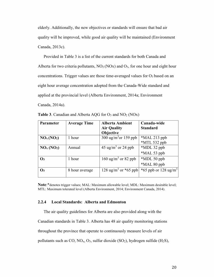
Provided in Table 3 is a list of the current standards for both Canada and
Alberta for two criteria pollutants, NO2 (NOx) and O3, for one hour and eight hour
concentrations. Trigger values are those time-averaged values for O3 based on an
eight hour average concentration adopted from the Canada-Wide standard and
applied at the provincial level (Alberta Environment, 2014a; Environment
Canada, 2014a).
Table 3. Canadian and Alberta AQG for O3 and NO2 (NOx)
Note:*denotes trigger values; MAL: Maximum allowable level; MDL: Maximum desirable level;
MTL: Maximum tolerated level (Alberta Environment, 2014; Environment Canada, 2014).
2.2.4 Local Standards: Alberta and Edmonton
The air quality guidelines for Alberta are also provided along with the
Canadian standards in Table 3. Alberta has 48 air quality monitoring stations
throughout the province that operate to continuously measure levels of air
pollutants such as CO, NOx, O3, sulfur dioxide (SO2), hydrogen sulfide (H2S),
Parameter Average Time Alberta Ambient
Air Quality
Objective
Canada-wide
Standard
NOx (NO2)
1 hour 300 ug/m3or 159 ppb *MAL 213 ppb
*MTL 532 ppb
NOx (NO2) Annual 45 ug/m3 or 24 ppb *MDL 32 ppb
*MAL 53 ppb
O3 1 hour 160 ug/m3 or 82 ppb *MDL 50 ppb
*MAL 80 ppb
O3 8 hour average 128 ug/m3 or *65 ppb *65 ppb or 128 ug/m3

21
total reduced sulfur, PM2.5 and PM10, dust and smoke, hydrocarbons (HC) and
ammonia (NH3) (CASA, 2014). The data retrieved from the air quality monitoring
stations are stored in a central repository for ambient air, the Alberta Ambient Air
Data Management System (AAADMS) or more commonly referred to as the
Clean Air Strategic Alliance (CASA) Data Warehouse. The CASA Data
Warehouse stores and archives time averaged hourly concentrations of air
pollutants, including specific gases and particulate matter, which are measured at
various urban and rural locations throughout Alberta via the Airshed monitoring
(CASA, 2014).
In the city of Edmonton, ambient air quality is monitored through a joint effort
that exists between the Alberta provincial government and various industrial
groups (City of Edmonton, 2014). Within and bordering Edmonton’s city limits
there are four ambient air-monitoring station, as well as one station designed
solely to measure particulate matter. All of these centralized monitors are
operated by Alberta Environment (City of Edmonton, 2014). Edmonton
participates with the Alberta Capital Airshed, a multi-stake holder which is a non-
profit organization that plays an essential role in air quality management and
monitoring. The Alberta Capital Airshed also acts as a portal for public
information on air quality (Alberta Capital Airshed, 2014).
Alberta Environment, Environment Canada, the City of Edmonton and
interested community members have worked cooperatively to create a network to
monitor ambient air quality and regulate industrial emissions (Alberta
Environment, 2009b). The non-profit group CASA.org collaborates with the

22
above key players to manage, provide guidance and address concerns regarding
air quality issues in local regions throughout the province (CASA, 2014).
In addition to centralized monitoring through the Alberta Airshed, there are a
few other methods and techniques used for monitoring air quality in Alberta
(Alberta Environment, 2013c). Other methods used for air quality monitoring
include intermittent monitoring and passive sampling. Intermittent air quality
monitoring is a system that monitors air pollutants as a 24-hour integrated
concentration on a six-day interval. Passive sampler air quality monitoring is
conducted by gathering air pollution samples from various locations on a monthly
basis, which are collected and analyzed for pollutant concentrations (CASA,
2014).
Air quality plays an important role in determining the health of the
environment. As literature reveals, the impact of industrialization,
commercialization and personal vehicular use has the potential to compromise
ambient air quality by increasing levels of NO2 (NOx) and O3. The air quality
standards that are set globally, nationally and provincially are applied by various
organizations, which strive to support optimum air quality. The objective of these
various organizations is to work collaboratively to provide preventative air quality
measures that are proactive in responding to the environmental impact of
continuous population and economic growth in urban and suburban environments.
2.3 Human Exposures to Pollutants
When considering human exposure to air contaminants in the outdoor/ambient
environment, certain factors must be considered prior to designing a human

23
exposure assessment. The factors which must be considered in accessing a
possible human exposure to air pollution in outdoor environments are:
1) meteorological conditions 2) degree of mobility of contaminants in the
atmosphere 3) source type, emission density and rate, and 4) distance/location of
an individual in relation to the generating source of pollution (NRC, 1991).
The National Academy of Sciences (1991) has determined that the
concentration of air pollutants in a given environment are generally dependent
upon a combination of factors in relation to types of activities operating within a
geographical location of interest. These environments of interest can be either
indoor or outdoor venues. The activities within these environments may be those
indoors as related to the types of household products used, or poorly ventilated
living spaces; and outdoors as related to high volumes of vehicular traffic or
industrial operations. The researchers concluded that the presence of air
contaminants within any environment is often the result of a series of multiple,
interactive and interrelated factors (NRC, 1991).
Concentrations of air contaminants within non-industrial indoor
environments, for example homes, may be dictated by the following factors:
1) the quantity, physical location and characteristics of the sources, 2) the diverse
characteristics of the specific built environment, including ventilation and
infiltration rates, 3) air mixing and penetration of outdoor contamination, 4)
meteorological conditions and 5) human and animal activity within the indoor
environment (NRC, 1991).
24
Further research conducted on exposure analysis by Ott (2007) describes the
concept of the full risk model as a tool to reduce the risk of adverse health
outcomes as a result of exposure to environmental pollutants. The full risk model,
as described by Ott (2007), has five foundational components that must be
considered when conducting an exposure analysis. The components include:
source of pollution, movement of pollutants, duration of exposure, dose
concentration of exposure, and the subsequent effect of the exposure. The main
emphasis of the science of exposure analysis is placed on the middle three
components: the movement of pollutants, to the exposure, to the dose (Ott,
2007a). A relationship between the source of environmental pollutants and their
effects on humans must be established. In this model pollutions sources are
considered to be either traditional or non-traditional in origin (Ott, 2007a).
Traditional sources are those that are obvious such as smoke stacks and
plumes exiting industrial operations and seen as directly entering the ambient air.
The public may associate pollution with the sight and smell of these stacks and
plumes and correlate these with a potential or current adverse health outcome for
those living and/or working in the area (Ott, 2007a).
Conversely, non-traditional pollutants are those that are not obvious to human
senses and are attributed to poorly-ventilated indoor environments or the use of
products such as household cleaning products, personal care items, and indoor
building products (Ott, 2007a). In comparison to traditional sources of air
pollution, these non-traditional sources of pollution may not be well regulated or
their environmental impact measured. These non-traditional sources may contain
25
highly reactive chemicals and when used in a closed environment, produce by-
products that can be more reactive than their predecessors. Human exposure to
non-traditional sources of air pollutants is the premise of the receptor-based
approach, known as exposure science (Ott, 2007a).
2.3.1 Exposure Science
Researcher and scientist, Wayne Ott (2007) stated that, in the past,
environmental policy on air quality was determined using traditional methods that
trace pollutants from the source to the human; the source oriented approach.
According to Ott (1985), determining an exposure/outcome at the human level is
extremely difficult, if not impossible, to trace using the source oriented approach.
Exposure science has provided a fundamental understanding of exposure by
narrowing its focus to the following components: the individual exposed, the
ways the pollutants reach these individuals and the potential adverse effects that
may result at the individual level (Ott, 2007a). Exposure science is a receptor-
based approach, a concept that is designed to trace exposure retrospectively from
the target to the source (Ott, 1985b).
Zhang et al. (2012) described the fundamental importance of collecting air
pollutant exposure data at the personal human level in order to set regulatory and
preventative risk assessment guidelines. Studies by several researchers have
indicated that people are more highly exposed to pollutants indoors in places such
as their homes, work and automobiles than in the ambient, outdoor settings (Ott,
2007a; Zhang et al., 2012).

26
Understanding the causal link between pollutant exposure and the effects at the
target is necessary in linking air pollutions sources with human health impact.
Exposure science is based on measuring human exposure to pollutants at the
personal level as related to the surrounding environment.
2.3.2 Source Based and Receptor Based Exposure
Tracing the cause and effect of pollution on the target organism can be
conducted in two ways: the concentration of pollutants can be measured at the
source and traced forward to the target (source based) or the concentrations of
pollutants can be measured at the target and traced backwards to source (receptor
based). The first looks at the source while the second focuses on the receptor.
The phrase ambient air quality refers to the quality of outdoor air in the
environment, pollutants can be measured based on their proximity to a source also
known as source-based exposure monitoring (NRC, 1991; Fenske, 2010). These
sources of emission are generally anthropogenic in nature and are often related to
areas of large volumes traffic and industrial operations (NRC, 1991; Fenske,
2010).
Receptor-based exposure refers to the concentration of pollutants that an
individual is exposed to in confined spaces and built environments such as
workplaces, homes and schools (Ott, 2007a). Indoors, air pollutants can be
released into the environment via store bought household cleaning products,
synthetic building material and inadequate ventilation of the built environment
(Lioy, 2010). Air quality indoors can be further compromised when the chemicals
from these sources combine to produce other by-products (Lioy, 2010). Many of

27
these near-field sources of pollutants can be found in the average home and can be
potentially harmful to the health of its occupants, especially small children, those
with respiratory ailments and the elderly.
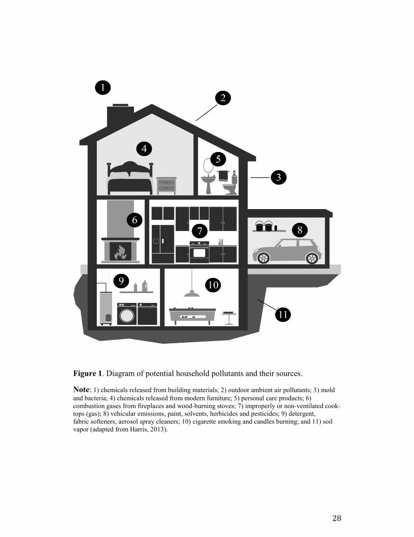
Figure 1 provides an example of some of the common and potentially harmful
household toxins people may be exposed to within their homes. The combinations
of various chemicals to form other chemicals is not easy to access as this process
of air mixing can be rapid and spontaneous. While there are current standards set
for maximum concentrations of the criteria pollutants, it is very difficult to
measure the effects of air mixing and moment to moment concentrations of other
harmful chemicals created by this process (Lioy, 2010).
28
Figure 1. Diagram of potential household pollutants and their sources.
Note: 1) chemicals released from building materials; 2) outdoor ambient air pollutants; 3) mold
and bacteria; 4) chemicals released from modern furniture; 5) personal care products; 6)
combustion gases from fireplaces and wood-burning stoves; 7) improperly or non-ventilated cook-
tops (gas); 8) vehicular emissions, paint, solvents, herbicides and pesticides; 9) detergent,
fabric softeners, aerosol spray cleaners; 10) cigarette smoking and candles burning; and 11) soil
vapor (adapted from Harris, 2013).

29
2.3.3 Direct Versus Indirect Approach to Measuring Human Exposure
In past history, the indirect and direct approaches to measuring air pollution
concentrations at the personal level have differed greatly. A new paradigm in air
monitoring has evolved due to the need to better understand the connection
between human exposure and pollution. This evolution in exposure concepts has
resulted in blending and integrating elements of both the direct and indirect
approaches in order to better measure human effects. A brief description of both
methods along with an outline of the benefits and limitations will be provided in
the following section.
Indirect methods of air quality monitoring involves the use of either passive or
active samplers to measure concentrations of pollutants in an environment of
interest (Zhang and Lioy, 2002). A time activity diary supplements the data
collected by the monitors and records artifacts as related to the specific
monitoring period. The time activity records or journals are used as a means of
recording circumstantial details during monitoring times based on the subjects’
activities patterns given time and space (Zhang and Lioy, 2002). Limitations of
the indirect method pertain to the questionable reliability of the sensors in
collecting accurate concentration levels of pollutants; and inconsistency and
inaccuracy in documentation by the subject of time activity information (Zhang
and Lioy, 2002).
The indirect approach is considered a modeling approach. A greater level of
uncertainty lies within the indirect method due to the inherent presence of
confounding factors and measures of bias. Research that employs indirect
30
approaches such as environmental monitoring, questionnaires, diaries and models
(i.e. fugacity or Monte Carlo method) does not provide data that either accurately
nor realistically represents actual personal exposure (Kindzierski, 2013).
In the past, the direct approach to measuring human exposure to air pollution
used either biological markers or personal air quality monitors to record pollutant
concentrations (NRC, 1991). Historically, personal exposure monitoring devices
were expensive, somewhat obtrusive, and limited in which pollutants they could
measure (NRC, 1991). New developments have produced small, light-weight,
inexpensive personal exposure monitors. These devices are highly technical with
the capabilities to measure a larger variety of pollutants (US EPA, 2012c).
Recent air quality research has incorporated the use of personal exposure
monitors with time activity diaries, a method that incorporates facets of both
indirect and direct approaches. As reported by Zhang and Lioy (2002) and Ott
(2007), time activity diaries have been designed and used as a way of recording
details pertaining to time, space, duration and conditions related to the activities
of the individual during monitoring periods. From these time activity diaries and
the quantitative data collected by the sensors, inferences can be drawn from a
sample of people as being representative of that area, and therefore, applied to a
larger population.
The direct approach of measuring human exposure to pollutants through use of
personal exposure monitoring has been found to be valuable. The rationale for this
can be explained in that personal monitoring provides for a realistic measurement
of exposure to near-field sources of pollutants based varied time activity patterns

31
of an individual or across a population of interest (Ott, 2007a). The approach was
also found to be valuable in providing quantitative measurements of ingestion
through food, water and dermal contact (Ott, 2007a). The direct approach is
receptor based and is often referred to as personal exposure monitoring (PEM)
(Kindzierski, 2013).
2.4 Types of Air Monitoring Methods
Studies across the world have delved into various techniques for measuring air
pollution levels from ambient air concentrations to near-field exposures at the
personal or individual level. While both centralized and personal exposure
monitors aim to measure concentrations of air pollutants, one is far-field source
based while the other is near-field source based.
In Houston, Carzola et al. (2012) tested ambient air ozone levels using a new
direct measurement technique labeled Measurement of Ozone Production Sensor
(MOPS). The MOPS was compared with two ambient air estimation methods for
measuring ozone, the calculated P(O3) and the modeled P(O3). The quantitative
comparison of the three methods showed that the measured and calculated O3
were similarly dependent on NO, whereas the modeled O3 was half that of the
measured O3. The researchers found that although the MOPS technique requires
more testing, the model shows potential to contribute to the understanding of the
chemistry required to produce O3 and, thereby impacting future air quality
regulatory actions (Carzola, et al. 2012).
East Asian countries have become increasingly concerned by atmospheric pollutant
concentrations in the ambient air due to growth of industry and vehicular use.
32
Itahashi, et al., (2013) studied episodic pollutant activities using the High Order
Decoupled Direct Method and Community Multiscale Air Quality Model
(HDDM-CMAQ) to clarify the source-receptor relationship (S-R relationship) of
O3 concentrations to NOx and VOC in regions of East Asia. The study determined
that far-field sources of NOx presented as the foundational precursor to increased
O3 levels in spring, summer and fall.
Due to a resurgence of interest in the need for further development of personal
air monitoring systems, the US EPA took action in the spring of 2009 (Gwinn et
al., 2011). This sparked a workshop gathering of parties which then led to the
formation of a mission with the mandate of estimating the benefits of reducing
hazardous air pollutants. From this, a list of hazardous air pollutants (HAPS) was
produced as a part of the Clean Air Act Amendments of 1990 as facilitated by the
US EPA (Gwinn et al., 2011).
The report by Gwinn et al. (2011) concluded that estimating benefits of
reducing air toxins is a multifactorial, complex process which required special
consideration and alternative methods of evaluation. Gaps in toxicological data,
uncertainties in dose/response extrapolation for high dose animal studies to low
dose human exposure, and limited ambient and personal monitoring data are
issues that required further clarification in order to fully understand the
mechanism of action and to enable effective regulation of HAPS (Gwinn et al,
2011).
In 2012, the US EPA held an Apps and Sensors for Air Pollution Monitoring
Workshop to facilitate collaboration between US EPA scientists and developers of
33
air monitoring sensors (US EPA, 2012d). The sensor developers came from
various parts of the United States and Europe in order to seek guidance from US
EPA scientists on issues pertaining to air monitoring. The emphasis was placed on
the development of effective personal air quality monitors that were sensitive,
accurate and easily calibrated. The goal of this collaboration was to promote
communication between the US EPA scientists and agencies dedicated to
exposure assessment sensors in order to improve technology, accuracy and
functionality (US EPA, 2012d).
Geyh et al. (1997) developed a small active O3 sampler, the Harvard Active
Ozone Sampler. The Harvard Active Ozone Sampler demonstrated a high level of
accuracy when compared with UV photometric measurements. Quantitatively, the
study found that the Harvard active ozone sampler/UV photometer showed an
accuracy of 0.94 to 1.00 and a level of precision equal to ± 4.1 to 6.5%.
Additionally, Geyh et al. (1997) concurred that this sampler performed equally as
well as the Time Exposure Diffusion Sampler, the only other O3 monitor of its
kind at the time (Geyh et al., 1997).
The studies discussed above provide evidence that centralized fixed-site
station monitoring and personal exposure monitoring have their respective roles in
air quality monitoring. While fixed-site monitoring provides for information on
general geographical air quality conditions; personal exposure monitoring
provides insight into exposures incurred at the receptor level, which vary greatly
from one person to the next. In order to correlate an adverse health outcome with
an exposure to air pollutants with any certainty, the fundamentals of exposure
34
science must be met. Personal exposure monitoring may provide the
exposure/dose information necessary to ascertain if and where a true health risk
exists.
2.4.1 Station Monitoring Versus Personal Monitoring
Studies have shown that centralized fixed-site monitoring may not be the
most representative of true exposure and that personal exposure monitoring of air
pollution may be the better solution. Personal monitoring incorporates elements of
exposure to air pollutants relating to activity and behavior patterns that are unique
to the individual which may not be well represented by fixed site measurements.
The following three factors are of interest when studying human exposure
patterns to air pollutants: ambient concentrations of pollutants, the combined and
cumulative effect of various indoor sources of air pollutants, and human time
activity patterns (Demokritou, et al., 2001). Centralized fixed-site monitoring has
been shown in the past to provide essential information and a general evaluation
of the air quality to provide evidence to support the development of regulatory
policy for promotion of environmental and public health.
In addition to addressing pollution levels in ambient air, the US EPA and
Environment Canada have also recognized the need to better understand the short
and long term effects of exposure to O3 and NO2 on a personal, individual level as
humans go about their daily lives (US EPA, 2012d; Environment Canada, 2013b).
The development of active, personal, real time monitors has improved vastly in
the last decade with devices constructed to be small, lightweight, cost effective
and easily powered (US EPA, 2012d).
35
In past studies, researchers in the United Kingdom studies the limitations of
fixed-site air quality monitoring. Sherwood and Greenhalgh (1960) discussed the
restrictions associated with fixed-site or static air sampling methods when
monitoring at occupational sites. The researchers explained their concerns in this
following statement: “it is sometimes necessary to determine the exposure of
workers who are engaged in a number of operations of working in a variety of
places. Under these conditions, air sampling at fixed points can give little
indication of exposure” (Sherwood and Greenhalgh, 1960, p. 127).
The National Academy of Science (1991) supported the need for receptor-
based monitoring of pollutants in their study by concluding that measuring air
pollutant concentrations was a fundamental part of predicting problems and taking
action in protecting both environmental and human exposures to pollutants. The
researchers concluded that air quality measurements must be conducted in both an
effective and accurate manner in order to optimize resources and provide
representative data for devising regulatory protocols that are reflective of real-
time activity exposures (NRC, 1991).
Nejadkoorki et al. (2011) addressed the issue of optimizing locations of
sampling station. In their research, a spatiotemporal approach was used to
measure actual human exposure to air pollutants. In fast-growing urban centers
such as Yzad, Iran, air pollution monitoring practices have focused on locating
monitors at several pollution ‘hot spots’. While these locations are acceptable for
determining maximum exposures and for estimating the degree of health risk, the
researchers questioned whether this type of monitoring practice was indicative of

36
actual, real-time daily exposure at the individual level (Nejadkoorki et al., 2011).
After comparing results from the spatiotemporal approach to ‘hot spot’
monitoring, researchers concluded that monitors when strategically placed in
areas most representative of urban exposure provided cost-effective and time
saving solutions in real-time air quality monitoring (Nejadkooki et al., 2001).
In existing epidemiological studies, the relationship between human health and
air pollutants has been researched by using centralized fixed-site monitoring as
the standard for quantifying exposure (Ozkaynak et al., 2013). Unfortunately, due
to variation in human activity patterns, station monitoring does not have the
capacity to account for the multifactorial nature of human exposure to air
pollutants (Ozkaynak et al., 2013).
Often air pollutants that are spatially heterogeneous, such as vehicular
emissions, are easily misclassified based on values reported at fixed-site monitors
(Ozkaynak et al., 2013). Station site monitoring data generally lacks information
based on spatial and temporal boundaries, providing an unclear picture of true
human exposure (Ozkaynak et al., 2013). In the study conducted by Ozkaynak
(2013) and similarly by Stienle (2013), the findings of both concluded that human
exposure to air pollutants was best represented through personal monitoring in
various geographical locations during different times of day.
A study by Spaeth (2002) reported that, traditionally, the practice of setting
regulations for air pollutants has been based on emissions rather than exposure
(Spaeth, 2002). In Spaeth’s (2002) report, the researcher states that air quality
assessment and regulatory bodies currently discount or completely disregard
37
human exposure as a major factor in setting standards. Human exposure levels to
toxic amounts of pollutants at a continuous rate have not been well represented.
As commonly reported in studies, Speath (2002) reconfirms that the average
person spends approximately 90% of time in indoor environments. With
regulatory standards for air quality being set based on ambient data, indoor
exposure which best represents personal exposure, has been entirely discounted.
Because of this, air quality standards are set with data that is based on real-time
concentrations of far-field ambient pollutants and not personal exposure to near-
field sources of pollutants (Spaeth, 2002).
Busy urban centers are thought to be focal areas for air quality monitoring;
these are presumed to be spots where human exposure to near-field, ambient air
pollutants may be significantly high. The Boston Personal Monitoring study
conducted in Boston by Ryan et al. (1986) tested human exposure to NO2 by using
personal exposure monitoring of a selected group of study subjects. The premise
of the study was to measure peoples’ exposure to NO2 based on unique time
activity patterns. Data collection involved the use of NO2 monitors, time activity
diaries and took into consideration the unique design of the home being
monitored.
The study by Ryan et al. (1986) concluded that people living within indoor
environments with gas ranges experienced a higher exposure (11 ppb) to NO2 in
comparison to those with electric ranges. Subsequently, the type of furnace fuels
used for heating the home, whether the home was single or multi-family and if
there was a microwave on-site had an impact on the level of indoor concentrations

38
of O3 + NO2 (Ryan, et al., 1986). The researchers did caution that these results
may be unique to this geographical setting and specific circumstances, stating that
findings may not be applicable to other similar exposure scenarios.
These studies discussed provide insight into some of the research that has
been conducted comparing far-field, source-based monitoring to near-field,
receptor-based monitoring. While these technologies have the capacity to measure
similar parameters their sources are different. Fixed-site monitoring provides for a
guide as to the air quality for a geographical area; while personal exposure
monitoring offers an insight into exposures incurred in areas where people spend
their time. At this time both monitoring approaches are necessary in assessing and
preventing potential environmental and human health risks in various settings.
2.4.2 Passive Monitors
Passive samplers (Figure 2) are commonly used in remote locations and
wilderness areas where there is no access to electricity. Passive samplers operate
without needing a power source. Subsequently, passive samplers are
advantageous because they are inexpensive, small and easy to use. They are
limited in that they may be effected by elements such as wind velocity,
temperature and relative humidity which may result in inaccurate measurements
of cumulative exposures in comparison to those collected by a continuous monitor
or an active sampler (Krupa and Legge, 2000).
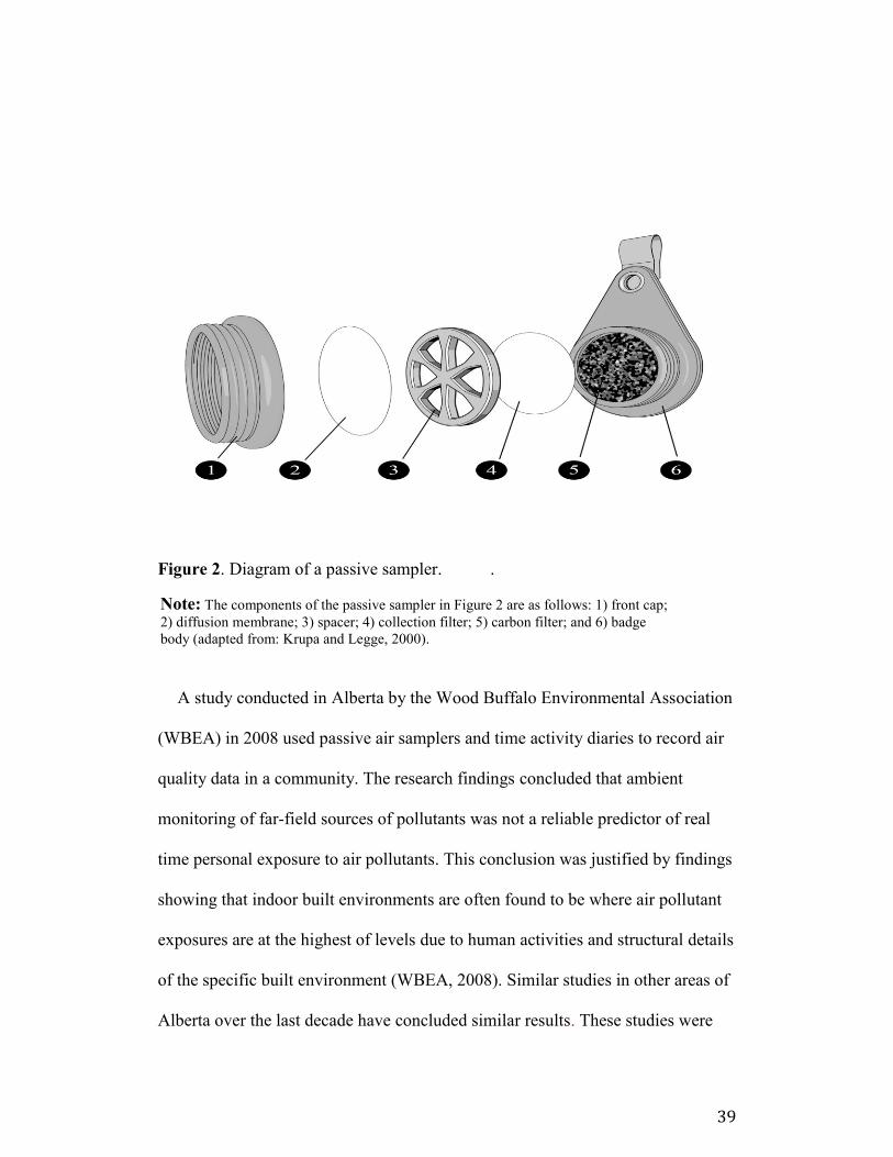
39
Figure 2. Diagram of a passive sampler. .
Note: The components of the passive sampler in Figure 2 are as follows: 1) front cap;
2) diffusion membrane; 3) spacer; 4) collection filter; 5) carbon filter; and 6) badge
body (adapted from: Krupa and Legge, 2000).
A study conducted in Alberta by the Wood Buffalo Environmental Association
(WBEA) in 2008 used passive air samplers and time activity diaries to record air
quality data in a community. The research findings concluded that ambient
monitoring of far-field sources of pollutants was not a reliable predictor of real
time personal exposure to air pollutants. This conclusion was justified by findings
showing that indoor built environments are often found to be where air pollutant
exposures are at the highest of levels due to human activities and structural details
of the specific built environment (WBEA, 2008). Similar studies in other areas of
Alberta over the last decade have concluded similar results. These studies were
40
conducted by the Wabamum and Area Community Association, the Fort
Saskatchewan and Area Community Association and the Grande Prairie and Area
Community Association due to their close proximity to industrial operations of
oil, gas and mining (WBEA, 2008).
Passive samplers work best at collecting concentrations of air pollutants when
conditions allow for free-flow, rapid air movement over a vast spatial area (Gaga
et al., 2012). The technology does not require active air movement through a
pump, rather airborne gases are collected through means of a physical process
such as diffusion or permeation through a membrane (Gaga et al., 2012).
A study conducted by Krupa and Legge (2000) found that passive samplers are
incapable of identifying short-term pollutant exposures or levels which exceed
regulated standards. Although statistical methods have been established to
effectively correct for these limitations of passive sampling, development of this
technology was ongoing. (Krupa and Legge, 2000). The authors conclude that the
use of co-located passive samplers was advantageous in studies focused on
regional level air quality and ecological risk assessments.
Yu et al. (2008) reviewed the development of passive samplers for detecting
NO2 levels in air, the sampling features of those currently available, and their
ability to monitor indoor/outdoor ambient as well as personal exposure to this
pollutant. The purpose of Yu et al.’s (2008) study was to aid researchers and risk
assessors in designing and streamlining field sampling strategies that are
representative of actual indoor/outdoor and personal exposures to air pollutants
(NO2).
41
In the United Kingdom, Lin et al. (2010) introduced a new directional passive
air sampler (DPAS) as a way of conducting continuous sampling of ambient air
for NO2 concentrations. The DPAS responded to directional wind changes and
velocities, showing potential of providing qualitative data. Diffuse passive
sampling is less expensive and requires fewer resources when compared with a
chemiluminescent analyzer (Lin et al., 2010). With the advent of some design
changes, the DPAS was found to be capable of sampling for air pollutants beyond
NO2. The researchers conclude that further testing and field trials of the DPAS
were supported.
2.4.3 Active Monitors
Research has demonstrated that active sampling is thought to be the method
of choice for use in measuring personal exposure to air pollutants. The technology
and usability of these devises has improved vastly, due to reduced size and
advanced capacities to store data, retrieve data and download data for future
analysis. Figure 3 provides for an example of just one of the new designs in active
samplers.
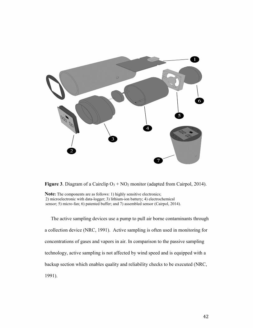
42
Figure 3. Diagram of a Cairclip O3 + NO2 monitor (adapted from Cairpol, 2014).
Note: The components are as follows: 1) highly sensitive electronics;
2) microelectronic with data-logger; 3) lithium-ion battery; 4) electrochemical
sensor; 5) micro-fan; 6) patented buffer; and 7) assembled sensor (Cairpol, 2014).
The active sampling devices use a pump to pull air borne contaminants through
a collection device (NRC, 1991). Active sampling is often used in monitoring for
concentrations of gases and vapors in air. In comparison to the passive sampling
technology, active sampling is not affected by wind speed and is equipped with a
backup section which enables quality and reliability checks to be executed (NRC,
1991).

43
New research and developments in technology for active sampling in
measuring various air pollutants has evolved in recent years. Small, lightweight
active samplers have been marketed for use in personal monitoring to measure
real-time exposure to pollutants in various settings. These setting may include
areas such as the workplace and/or residential environments (US EPA, 2012d).
An important aspect of this evolving technology has been to create monitors
that are easy for people to wear, simple to use and provide instant warnings when
exposures are high. These particular design features aim to engage people and
create awareness of issues pertaining to their exposure to pollutants in the local
environment with which they spend the majority of their time (US EPA, 2012d).
By engaging the public through the use of these active air quality samplers, the
public are able to develop an awareness of air pollution as it pertains to the health
of their immediate environments (US EPA, 2012d).
In particular, recent developments by Cairpol have resulted in the production of
small, personal active air monitors that measure a sum of the continuous
concentrations of O3 and NO2 on a real-time capacity (Cairpol, 2013). In a
technical report conducted by the Joint Research Center (JRC) in Europe, the
sensors were evaluated for functionality in comparison to other similar sensors, as
well as performance in laboratory and field settings. After a series of tests, the
researchers determined that the Cairclip O3 + NO2 was found to have met the Data
Quality Objective (DQO) of indicative method of the European Directive (JRC,
2013). A more in-depth discussion on the Cairclip O3 + NO2 sensors will be
provided in Chapter 3.

44
2.4.4 Personal Monitors
Currently, the three most common methods of personal exposure monitoring
are: personal air monitoring, personal dietary monitoring and reconstruction of
exposure based on findings from biomarkers (Kindzierski, 2013). Personal
exposure monitoring is considered the ‘Gold Standard’ and the most reliable
method of attaining accuracy in the concentrations of a pollutant(s) received by
the human in order to ascertain if a risk exists (Kindzierski, 2013).
Personal air monitors use either passive or active technology, depending upon the
instruments design, to measure pollutant concentrations at the receptor level. As
described briefly, new designs of personal exposure monitors, such as the Cairclip,
have resulted in the emergence of small, highly sensitive, low powered, cost effective
and portable devices worn by a person at or around the breathing zone (NRC, 1991).
Initially, the focus on air quality was placed on developing national outdoor
monitoring systems for criteria pollutants with little interest focused on personal
exposure monitoring (US EPA, 2012d). Regardless of the beliefs of some that felt
that centralized monitoring was the best option, researchers continued to study
and gain knowledge on personal exposure monitoring.
The result of research conducted in the 1970’s by Granger Morgan and
Leonard Hamilton showed that the efficacy of personal monitors was found to be
feasible due to improvements in technology (Morgan and Morris, 1976). These
findings set the stage for further testing and development of sensors that were
designed to better measure near-field exposure to pollutants (Morgan and Morris,
1976).
45
Simultaneously, the National Academy of Science (NAS) (1977), upon the
request of the United States Congress, reviewed the scientific methods of the US
EPA. Findings in their nine volume report contained a section titled
‘Environmental Monitoring’ (NAS, 1977). The report confirmed that the
organization was not participating in further development of personal air quality
monitors. In response to the US EPA’s stance on further development of personal
monitoring technologies, Wallace (1982) vocalized his concern. Wallace (1982)
aimed to inspire further research and developmental strategies for improving
personal air monitoring devices by making this statement: “the Agency is not
currently developing personal air quality monitors. By equipping a controlled
sample of people with these portable sampling devices, the concentration of the
pollutants to which they are exposed could be measured. There is evidence to
challenge a common objection that personal monitors are technologically
impracticable. Prototypes have been developed to detect several air pollutants at
levels near ambient concentrations” (Wallace and Ott, 1982).
The above words written by Wallace were intended to promote development
and improve the technology of personal active air monitoring devices to enhance
reliability of air quality data and to act as an adjunctive tool exposure
assessments. Upon these recommendations, the US EPA responded by sponsoring
a symposium and allocating funding in order to instigate development of personal
air quality monitors (Wallace, 2007b).
As a result of forward thinking on the part of the NAS and the support of the
US EPA, developmental advances of personal monitoring devices have evolved to
46
a point where air quality issues can be pinpointed with far greater accuracy
(Wallace, 2007b). Personal monitoring has determined that the main sources of
exposure of humans to pollution are those that are close to the person (near-field
sources) that are incurred during various activities as a person moves about their
day.
Cairpol, the manufacturer of a new technology in personal exposure
monitoring, is one of many companies engaged in further, advanced development
in air quality monitoring. The European based company has produced active
samplers that are designed to measure personal level exposure to various gases
including one that measures a sum of O3 + NO2, named the Cairclip O3 + NO2
(Cairpol, 2014).
Currently, limited research has been conducted that tests the accuracy and
reliability of these sensors in both field and laboratory settings. The study released
from Europe and conducted by the JRC in 2013 tested the Cairclip O3+NO2 to
evaluate their performance and degree of measurement uncertainty in laboratory
and field settings (Spinnelle et al., 2013). The sensors were evaluated in relation
to the DQO, a guideline established to promote the health of humans and
ecosystems, set by the European Air Quality Directive (Spinnelle et al. 2013).
The aim of the study by the JRC was to demonstrate whether or not the
Cairclip sensor satisfied the DQO of 60 nmol/mol (60 ppb) for O3 Indicative
Methods at the target level limit values (LV) (Spinnelle, et al., 2013). The DQO
defines target level for O3 as a fixed level that is aimed at avoiding long-term
harmful effects on human health and/or the environment as a whole. The term LV
47
is defined by the DQO as a concentration limit is set based on scientific findings,
aimed at avoiding, preventing or reducing the harmful effects on human health
and/or environment as a whole. These LVs for pollutants pertain to concentrations
reached within a set period of time and once reached are not be exceeded
(European Commission, 2014a). In reference to a LV value of 60 ppb, the
research found the Cairclip O3 + NO2 sensor satisfied the DQO Objective of
indicative method of the European Directive. Field testing, which challenged the
Cairclip O3 + NO2 sensor against the centralized monitors in France, showed a
relative expanded uncertainty of 20%, a value very similar to the manufacturer
determined value of 19% (Cairpol, 2014).
A fundamental part of the European Commission’s study involving the
Cairclips was to challenge the integrity and accuracy of the sensors given
different environmental settings and conditions. The Cairclips were tested in both
a laboratory and a field setting for their efficacy in measuring levels of O3 and
NO2. In the field, researchers tested the sensors for O3 monitoring in
suburban/rural settings. The sampling sites for NO2 were selected to represent
high density urban areas, characterized by large volumes of traffic and population
density (Spinnelle et al., 2013).
In order to determine the Cairclip’s integrity to collect concentrations of O3
and NO2 equally, researchers placed the sensors in settings that were favorable for
collection of the individual gases. By doing this, the researchers were able to
conclude that in both laboratory and field settings the Cairclip showed a
heightened sensitivity or affinity to concentrations of NO2 over O3. Because of
48
this, the researchers determined that the sensors would act to underestimate levels
of O3 when monitoring in areas where both gases are equally and simultaneously
high (Spinnelle et al., 2013).
In addition to the findings discussed above, the JRC found that on average the
response time of one and a half minutes, the fall time of less than one minute and
the rise time of approximately two minutes of the Cairclip O3 + NO2 sensor were
congruent with that originally reported by the manufacturer. The sensor did not
experience short or long term drift, were not sensitive to temperature changes and
did not report extreme effects when concentrations of O3 changed (Spinnelle et al.,
2013).
Limitations of the sensors were found to be that the Cairclip had the potential
to become desensitized or deconditioned post-calibration if not exposed to similar
concentrations in a new setting. Deconditioning of the Cairclip was thought to
occur when the sensor was placed in new environmental conditions with lower
concentrations of O3 and NO2 or if the battery charge was lost (Spinnelle, et al.,
2013). The researchers also believed the sensors to be overly sensitive to
concentrations of NO2 affecting its reliability in measuring accurate O3 levels
(Spinelle, et al., 2013).
Different methods, such as fixed-site monitors, stationary microenvironment
monitors and personal monitors, may be used to measure concentrations of air
pollutants. When these methods are compared and rated in terms of accuracy,
personal monitoring has been found to be, by far, the most effective and realistic
method for attaining individual exposure information (Steinle et al., 2013). This

49
said, current policy on air quality remains set based on centralized fixed-site
monitoring, suggesting that the technology of personal monitoring has not quite
reached a consistently reliable level in order to replace station monitoring. Better
yet, as the personal exposure technology improves these have the potential to be
an essential adjunct to centralized monitoring.
2.5 Components of Personal Exposure Monitoring
Humans have a unique way of interacting within their environments.
Because on this, exposure to pollutants varies from person to person based on the
variety of activities people engaging in and the areas with which they spend time.
Statistically, humans are found to spend 90 percent of their day in a variety of
indoor environments, be it at work, home, school or other public establishments.
A person’s ethnic background, social connection, environment and
socioeconomics are key elements the social determinants of health. Often these
factors dictate the quality of one’s health and are predictors of lifestyle habits and
daily activity patterns.
Personal exposure monitoring as reported by Spengler and Soczek (1984) is
best represented by the use of a combination of personal exposure sampling
supplemented with individual time activity diaries. When human health is of
interest, the focus of monitoring is to test the environments which people spend
the majority of their time. By monitoring indoor environments of a person or a
group of persons, researchers are collecting air quality data most representative of
actual exposure (Spengler and Soczek, 1984).
50
Although this research does not expand in detail with regards to the social
determinants of health, it is important to make the connection that various lifestyle
choices and habits of people may be predetermined by socioeconomic status and
social conditioning. These lifestyle habits, such as cigarette smoking, can
inadvertently result in exposures to higher levels of indoor air pollutants on an
everyday basis; and potentially impact the quality of an individual’s health in the
long term. As reported in a study by O’Neill et al. (2003), the researchers
reaffirmed that exposure to levels of air pollution varies based on socioeconomic
circumstances. Socioeconomic status and air pollution are found to be
confounding factors to increased rates of morbidity and mortality from respiratory
ailments (O’Neill et al., 2003).
2.5.1 Real Time Monitoring and Time Activity Diaries
Time activity may be defined as the spatial and temporal boundaries, which
define how people spend their time throughout the day (Steinle et al., 2003). For
purposes of studying human exposure to air pollutants, knowing where people
spend their time, and the activities they engaging in during this time are the
primary determining factors in assessing individual exposure/risk potential. In the
case where pollution is sufficiently high and duration of human exposure is long,
an exposure will occur (Kindzierski, 2013).
In order to obtain data on activities patterns of people; tools such as time-
activity diaries (TADs) and questionnaires have become essential to information
gathering (Lioy, 2010). When managed with continuity and detail, data received
51
from TADs and questionnaires can be a critical tool used to correlate exposure to
specific locations, times and activities (Steinle et al., 2013).
Real-time air monitoring devices are those that record pollutant
concentrations as they occur at the receptor of interest. Research conducted by
Adam et al. (2009) tested a high resolution, spatio-temporal sampling method for
assessment of personal exposure to particulate matter. The researchers conducting
the study concluded that this method was effective and applicable to measuring
real-time personal exposure all contaminants, including particulate matter.
The future of real-time, near-field source exposure monitoring shows potential
for providing a better understanding of personal exposure. The advent of new
technology and design features that encourage personal compliance will assist in
establishing where exposure to pollution may be high based on time and location
of the individual.
2.5.2 Microenvironments
Microenvironments may be described as any physical space where people
spend time engaging in certain activities at various frequencies and for certain
durations of time (Steinle, et al., 2013). Measuring air quality within certain
microenvironments where people spend time is beneficial to identifying exposure
to pollutants in certain built environments (Steinle, et al., 2013). Although air
monitoring of indoor or contained microenvironments may not be as effective as
personal exposure monitoring, it has been shown to be more representative of
individual exposure that that of outdoor monitoring (NRC, 1991).
52
A condition known as ‘sick building syndrome’ has become a health concern
for people living and working in indoor environments with compromised air
quality (Wallace, 1997b). The condition can be related to structural issues of the
built environment such as inadequate or poorly designed ventilation, off-gasing of
synthetic materials used in carpets and furnishings, and interruption in air flow
created by room dividers (NRC, 1991; Wallace, 1997b).
A study by Carvalho et al. (2009) tested air quality on public transportation
due to the high number of commuters using this form of transportation in busy
urban centers. In the study, the researchers introduced a mobile air monitoring
station that was attached to mass transport vehicles such as buses and trains as a
way of measuring air pollutant concentrations in various urban areas at various
times. The mobile monitor was developed as a way of informing commuters of
their level and duration of exposure to pollutants in various areas of a busy
metropolitan setting. Researchers concluded that the mobile station design was
advantageous over fixed site air monitoring as it allowed for real-time air
monitoring in specific microenvironments close to pollutant source (Carvalho et
al., 2009).
2.6 Summary
The information in Chapter 2 aimed to provide for a background discussion
and overview of the air pollutants O3 and NO2, current and past monitoring trends
and tools, details of exposure science and components of air quality monitoring.
The purpose of the research presented in this study is to address the level of
accuracy and precision of the Cairclip sensors in the city of Edmonton in

53
reference to the Edmonton south centralized station; and to test the variation in
exposure to pollutants that exists between monitoring near-field sources at the
receptor and far-field sources as recorded by centralized monitoring.
The study intends to test new technology in active sampling by challenging its
ability to measure pollutants at a personal, real-time capacity given diverse
exposure scenarios. The information may be beneficial in determining which
urban environments the Cairclip sensor functions best and determining areas that
may be considered ‘hot spots’ of pollutants, which may pose potential health
risks to humans and diverse ecosystems.
54
3 METHODOLOGY
3.1 Basis of Study
Monitoring of air pollutants in Edmonton, Alberta is conducted through the
Alberta Airshed’s four fixed-site monitoring stations located throughout the city.
These monitoring stations assess air concentration of criteria pollutants and
particulate matter hourly. The daily Air Quality Health Index (AQHI) is set based
on data collected at fixed-site monitoring stations and is available for public
access. While measurements of ambient air pollutants by means of centralized
monitoring is beneficial for providing a generalized rating for daily air quality and
setting policy, studies have shown that this type of monitoring does not well
represent air pollutant exposure at the personal or individual level.
In this study, conducted from July 2013 to January 2014, new technology in
personal air quality monitoring devices was tested in a two-phase model design.
Phase one of the study tested: 1) the Cairclips’, a personal exposure monitor
(PEM), level of accuracy in measuring continuous concentrations of O3 and NO2
in ambient air in comparison to the Alberta Airsheds fixed site monitor at
Edmonton’s south station, and, 2) to compare the level of precision between the
PEM’s when used in a field setting. Phase two of the study measured near-field
sources of pollution at a personal level also referred to receptor based exposure.
As part of phase two, the person’s residence was monitored in both indoor and
outdoor capacities for comparison.
The following sections provide a description of the air monitoring devices used
in the study, details regarding the design of the two phases of the study, the type
55
of data collected, procedures for determining precision and accuracy of devices
and data inclusion and exclusion criteria based on critical analysis of the data
collected (Alberta Environment, 2006e). The data collected in this study is
intended to evaluate the efficacy and reliability of new, innovative designs of
active sampling air quality monitors as a future means of enhancing reliability in
measuring human exposure to air pollution.
3.2 Description of Monitors
The US EPA (2012d) reported that the ongoing development of personal
monitoring devices shows a promising future in providing alternatives to current
air monitoring practices that may: 1) reduce costs and decrease the demand for
manpower, and 2) promote public engagement and involvement in issues of air
quality that may affect both human and environmental health (US EPA, 2012d).
New technology in active air samplers, as exemplified by the Cairclip, aim to
provide data on exposures to near-field sources of pollutants measured at the
human level. This may prove advantageous as a means of engaging people in
understanding the importance of air quality in order to alter behavior that may
further contribute to pollution levels. Also because indoor air quality poses the
largest threat to human health, personal monitoring of these spaces aims to
provide a real view of true risk.
Several companies have produced personal exposure monitoring devices that
are targeted at measuring near-field pollution at the receptor level and are
designed to measure various types of air pollutants. The Cairclip was designed
and manufactured by Cairpol, a company in Mejannes-les-Ales, France (Cairpol,
56
2014). The unobtrusive, small, lightweight design of the Cairclip active sampler
makes them more compatible for use on a personal level than that of past personal
air monitoring devices. Traditionally, personal active samplers have been quite
large and too cumbersome to be worn for long periods of time.
The Cairclip is designed with a LCD screen that provides time of day, battery
life, as well as instant readouts and warnings based on detection levels of air
pollutants by concentration and exposure time (Cairpol, 2014). The Cairclip is
capable of providing four different warning levels depending upon the
concentration of pollutants detected. The battery is lithium-ion with an integrity of
up to 24 hours. The device can be easily recharged using a computer via a USB or
an electrical outlet with an adapter, which is supplied by the company.
In order to ensure longevity and safety of the sensors, the operating guidelines
as devised by the Cairpol manufacturer were adhered to strictly (Appendix A).
For the entire duration of phase one and two, the monitoring was conducted on
days that met these climatic conditions: 1) the temperature range of -20 to +40
degrees Celsius, 2) a relative humidity ranging between 10 to 90%, and 3) an
atmospheric pressure of between 0.10 and 2.00 MPa. This information is provided
in a copy of the Cairclip technical data sheet compiled by Cairpol in Appendix A.
The Cairclip sensor has the capacity to save data for up to 20 days post-
monitoring. Once the data sampling time was complete, the data was downloaded
from the Cairclip sensor directly onto a PC laptop computer via a program called
Cairsoft. The Cairsoft software is currently compatible for use with PC computers
and is a uniquely designed computer program, specifically used for data retrieval
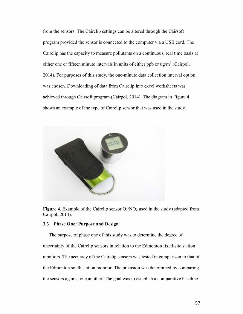
57
from the sensors. The Cairclip settings can be altered through the Cairsoft
program provided the sensor is connected to the computer via a USB cord. The
Cairclip has the capacity to measure pollutants on a continuous, real time basis at
either one or fifteen minute intervals in units of either ppb or ug/m3 (Cairpol,
2014). For purposes of this study, the one-minute data collection interval option
was chosen. Downloading of data from Cairclip into excel worksheets was
achieved through Cairsoft program (Cairpol, 2014). The diagram in Figure 4
shows an example of the type of Cairclip sensor that was used in the study.
Figure 4. Example of the Cairclip sensor O3/NO2 used in the study (adapted from
Cairpol, 2014).
3.3 Phase One: Purpose and Design
The purpose of phase one of this study was to determine the degree of
uncertainty of the Cairclip sensors in relation to the Edmonton fixed-site station
monitors. The accuracy of the Cairclip sensors was tested in comparison to that of
the Edmonton south station monitor. The precision was determined by comparing
the sensors against one another. The goal was to establish a comparative baseline

58
of data to determine the degree to which the sensors performed in comparison to
the ambient station (accuracy) as well as how well each sensor performed in
comparison to one another (precision).
3.3.1 Location and Deployment of Cairclip Sensors for Phase One
Phase one of the study involved co-locating the Cairclips with Alberta
Environments’ NAPS station monitor located in south Edmonton. The Edmonton
South Station monitors for several types of pollutants such as carbon monoxide
(CO), sulphur dioxide (SO2), nitric oxide (NO), total oxides of nitrogen (NOx),
NO2, O3, total hydrocarbons, non-methane hydrocarbons, as well as PM2.5 and
PM10 (CASAdata.org, 2014).
The Edmonton South Station monitor was chosen because of its close
proximity to the University of Alberta. It is presumed to represent air quality in
residential areas of the city. The geographical coordinates for the site are as
follows: latitude: 53.500139, longitude: 113.526056, elevation: 681.0
(CASAdata.org, 2014). The monitoring station is located at 6240-113 Street,
Edmonton, Alberta, between the Alberta School for the Deaf and the south
extension of the light rail transit (LRT) lines. The geographical location of the
station monitor in relation to the University of Albert farm and the South Campus
LRT station are displayed in Figure 5. The photograph in Figure 6 was taken to
provide a visual perspective of the design of the fixed station, as well as to give a
visual illustration of the surrounding environment. Arrangements were made with
Shelley Morris of Alberta Environment to acquire a key for access to the NAPS
station monitor compound.
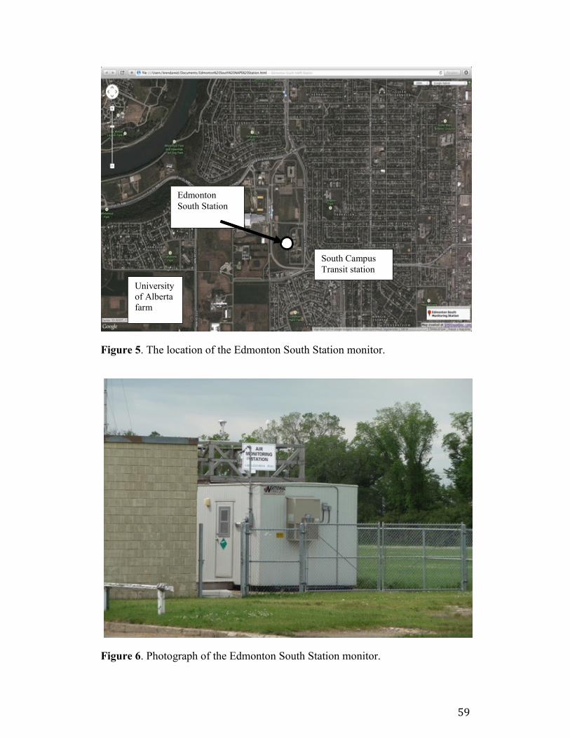
59
Figure 5. The location of the Edmonton South Station monitor.
Figure 6. Photograph of the Edmonton South Station monitor.
Edmonton
South Station
University
of Alberta farm
South Campus Transit station

60
The shelter for the Cairclip sensors consisted of a circular hood with a
circumference of 56.5 centimeters (cm) in order to provide the sensors sufficient
protection from wind and rain. The hood was attached to a long metal pole,
measuring 123 cm in length. Directly beneath the hood was a structure that was
comprised of four arms enabling attachment of four sensors, one on each arm with
all components attached at the top with a screw. The assembled shelter was then
fastened to a corner of the wood railings on top of the Edmonton south station
monitor. A variety of clamps, brackets and screws were used to firmly secure the
apparatus against inclement winds, and adverse weather conditions (Figure 7).
Figure 7. Hardware used to secure the shelter for the Cairclips.
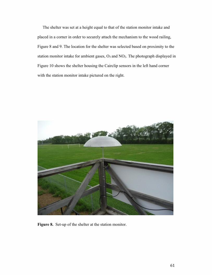
61
The shelter was set at a height equal to that of the station monitor intake and
placed in a corner in order to securely attach the mechanism to the wood railing,
Figure 8 and 9. The location for the shelter was selected based on proximity to the
station monitor intake for ambient gases, O3 and NO2. The photograph displayed in
Figure 10 shows the shelter housing the Cairclip sensors in the left hand corner
with the station monitor intake pictured on the right.
Figure 8. Set-up of the shelter at the station monitor.
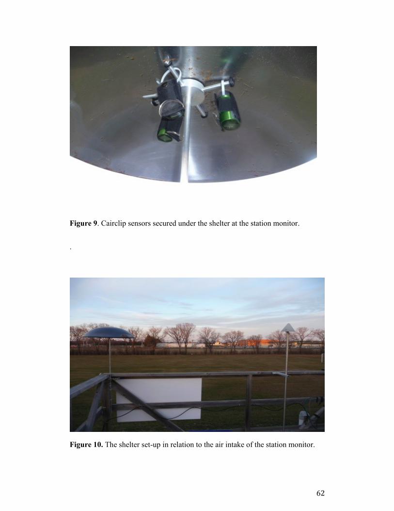
62
Figure 9. Cairclip sensors secured under the shelter at the station monitor.
.
Figure 10. The shelter set-up in relation to the air intake of the station monitor.

63
3.3.2 Time of Day and Duration of Data Collection for Phase One
Deployment times for collection of air quality samples were determined by
reviewing previous data collected for air monitoring sites across Alberta and
within Edmonton city limits. A study discussing ambient air trends conducted by
McCullum et al. (2004) provided temporal data on daily concentration levels of
O3 and NO2. The study showed peaks and valleys of concentrations for all days of
the week and for several areas in Edmonton and across Alberta. As the Cairclips
were capable of collecting data for 24 hours, time frames for data collection were
eight to twelve hours in length in order to cover peak times of concentrations of
O3 and NO2 as related to rush hour traffic and in consideration of climatic
conditions (McCullum et al., 2004; Alberta Environment, 2012d). Once the
monitoring was completed, the sensors were removed, data was downloaded onto
a laptop computer and the sensors were recharged overnight. Twenty-five days of
data were collected during the course of Phase one of this study.
3.3.3 Quality Control and Quality Assurance Experiments
In order to validate study results and safeguard against inconsistencies between
sensors, elements of quality assurance and control were essential in all areas
throughout the duration of the research project. This involved downloading of
data software; the development of a charging station to ensure optimal battery life
during monitoring times; the numbering of the sensors from 1 to 4 for tracking
purposes; and, fabrication and set up of an outdoor shelter to safeguard against
damage due to wind and rain. Log sheets were developed in order to record entry
and exit times into the Edmonton south station compound. Additionally, the log
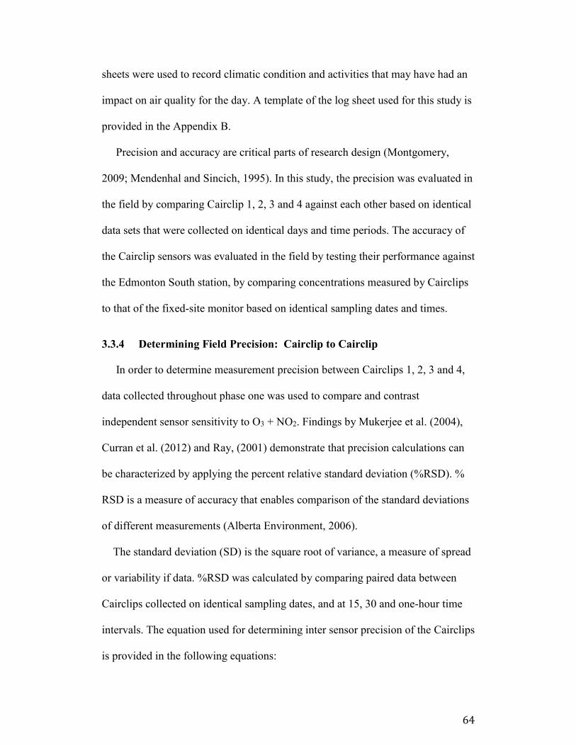
64
sheets were used to record climatic condition and activities that may have had an
impact on air quality for the day. A template of the log sheet used for this study is
provided in the Appendix B.
Precision and accuracy are critical parts of research design (Montgomery,
2009; Mendenhal and Sincich, 1995). In this study, the precision was evaluated in
the field by comparing Cairclip 1, 2, 3 and 4 against each other based on identical
data sets that were collected on identical days and time periods. The accuracy of
the Cairclip sensors was evaluated in the field by testing their performance against
the Edmonton South station, by comparing concentrations measured by Cairclips
to that of the fixed-site monitor based on identical sampling dates and times.
3.3.4 Determining Field Precision: Cairclip to Cairclip
In order to determine measurement precision between Cairclips 1, 2, 3 and 4,
data collected throughout phase one was used to compare and contrast
independent sensor sensitivity to O3 + NO2. Findings by Mukerjee et al. (2004),
Curran et al. (2012) and Ray, (2001) demonstrate that precision calculations can
be characterized by applying the percent relative standard deviation (%RSD). %
RSD is a measure of accuracy that enables comparison of the standard deviations
of different measurements (Alberta Environment, 2006).
The standard deviation (SD) is the square root of variance, a measure of spread
or variability if data. %RSD was calculated by comparing paired data between
Cairclips collected on identical sampling dates, and at 15, 30 and one-hour time
intervals. The equation used for determining inter sensor precision of the Cairclips
is provided in the following equations:
65
% RSD = (SD
�̅�) * 100%; and SD = √
∑ x′−x"
2 ∗n (Eq.1) & (Eq.2)
where, SD is the standard deviation from paired Cairclip data and 𝑥 = the arithmetic
average of x′.
3.3.5 Determining Field Accuracy: Cairclips to NAPS Station Monitor
To date, there has been one published study conducted in Europe by the JRC
where the Cairclip sensors have been challenged for accuracy and precision in a
similar capacity to this study (Spinelle et al., 2013). Due to the limited amount of
knowledge about the Cairclip sensors, it was an imperative part of this study to
test their accuracy against a reference point that was representative of the air
quality in Edmonton. Although the station monitors record concentrations of
O3 + NO2 from a fixed-site and are limited to measuring far-field sources, they
were considered to be the best reference for air quality data.
Upon completion of phase one, data collected was assessed for accuracy by
comparing each Cairclip with the Edmonton south station monitor data based on
identical times and dates. Alberta Environment provided one, ten and sixty minute
data for specific dates throughout the period from July 29 to November 1, 2013.
The analysis for phase one using data collected at one minute time intervals to
calculate 15 and 30 minute, and one hour time average concentrations of the sum
of O3 and NO2.
For purposes of this study and in accordance with literature, accuracy was
calculated using the mean absolute percent difference (MAPD) (Curran et al.,
2012; Ray, 2001) using the following equation:
66
MAPD = [(
P−C
P)
n] * 100 (Eq.3)
where, P is the combined concentrations of O3 + NO2 measured in ppb from the
NAPS Edmonton South station monitor; C is the reported time weighted concentration
of O3 + NO2 measured in ppb by the Cairclips; and n is the sample size or number of
paired data.
3.3.6 Data Selection Criteria
All of the data gathered from the Cairclip sensors was screened and analyzed
in order to determine which data sets met inclusion or exclusion criteria. As noted
above, accuracy was determined by comparing the Cairclip data to that of the
station monitor, while precision was determined through comparison of paired
Cairclip data. The following selection criteria were applied to the data:
The active sampler data had to have been collected by the Cairclip and
recorded at one minute, continuous time intervals.
The date, time and length of monitoring times for all four of the Cairclip
sensors was consistent with that of the Edmonton South station monitor.
Incomplete data from station monitor, due to power outages or maintenance,
during monitoring times with co-deployment with Cairclips resulted in
removal of those time-weighted values from data sets.
Reference data for phase one of the study from station monitor was
restricted to that recorded at the NAPS Edmonton South station.
67
3.3.7 Datasets Group One, Two and Three for Comparison
Upon completion of screening data on the specified criteria, the data sets were
evaluated for presence of outliers. In phase one, accuracy data and precision data
were graphed showing Cairclip vs. Edmonton south station monitor or Cairclip vs
Cairclip, respectively. In both accuracy and precision graphs, linear regression
lines were adapted to the points with R2 equations and calculations provided.
Upon consulting with specialists within the School of Public Health at the
University of Alberta, Drs. Yutaka Yasui and Gian Jhangri (personal
communication April 4, 2014), it was recommended to remove any data points
that were visually spurious when analyzed in linear regression. The removal of
outliers was a carefully thought out process that aimed to capture quantitative
comparisons of the Cairclip that were reflective of its capacity to measure
concentrations of far-field sources of O3 + NO2 in comparison to the station
monitor.
Subsequently, a second outliers test was applied using calculated standardized
residual data to determine any data points that lay beyond ±2SD of the mean. Any
data points beyond this were considered outliers and removed from the data sets
(Currie et al., 1994; Curran et al., 2012). The accuracy and precision results of: 1)
all screened data, 2) screened data with visual outliers removed and 3) screened
data with outliers removed beyond m±2SD, are presented for comparison in
Chapter 4.

68
3.4 Phase Two: Purpose and Design
Phase two of the study was designed to measure selected outdoor geographical
locations and indoor environments throughout the city of Edmonton. Firstly, the
purpose of monitoring in certain locations was to determine if areas with high
volumes of traffic, which coexist with human activity, may be potential areas of
high exposures to O3 + NO2. This involved monitoring outdoors at intersections in
core urban areas of Edmonton and while commuting on public transit. Secondly,
to monitor indoor environments located in close proximity to intersections with
high volumes of traffic that were equipped with gas ranges and fireplaces, etc. to
measure the levels of O3 + NO2 in these locations.
The sensors were assigned to a specific scenario: indoor, outdoor or personal
and remained assigned to the same setting for the duration of the study. The
sensors were assigned as follows: 1) Cairclip 2 was placed inside the home,
2) Cairclip 3 was placed in the backyard of the home using the same protective
shelter used in phase one, and 3) Cairclip 1 and 4 were assigned to be worn by a
person.
Monitoring times for phase two varied somewhat in accordance with changing
time activity patterns from day to day. The monitoring times ranged from 8 hours
to a maximum of 12-hours to safeguard sufficient battery life and to ensure the
provision of the best possible measurement accuracy of the sensors. Outdoor and
indoor monitors were deployed daily at the same time as the personal monitor to
be worn by the individual. A time activity diary was carried with the person and
records identifying geographical location along with duration of time spent in the

69
specific area were recorded. Any other artifacts of interest that were thought to
potentially affect data collections were also noted.
As mentioned, the focus of phase two of the research study aimed to measure
exposure to air pollutants, O3 and NO2, during daily life activities. For this reason,
the selection of exposure scenarios were done with the intent to reflect changing
exposures to pollutants as an individual’s activity and location of those activities
changed. Data collection intervals aimed to capture diurnal patterns such as times
of peak traffic flow when vehicular emissions are high. The timeline for phase
two extended from September, 2013 to January, 2014.
The scenarios selected for the personal exposure monitoring were chosen to
be representative of daily life patterns. The scenarios were selected to reflect a
person’s diurnal patterns and incorporated monitoring activities when: 1)
commuting by foot in core areas of the city; 2) commuting by train and bus; and
3) inside public indoor environments adjacent to high volume vehicular traffic.
Figure 11 highlights the areas of monitoring as related to the above scenarios
throughout the city of Edmonton.
Once data collection was completed, the results were compared to data from
the Edmonton South and Edmonton Central station monitors. The location of the
Edmonton Central station monitor is in the downtown core at 10255 – 104th Street
with co-ordinates of 53.54449, -113.49893; this station is designed to be
representative of measurements of pollutant concentrations in a densely populated
urban environment of the city (Environment Canada, 2013c). Pedestrian counts,
where available, were used to determine the volumes of people in close proximity
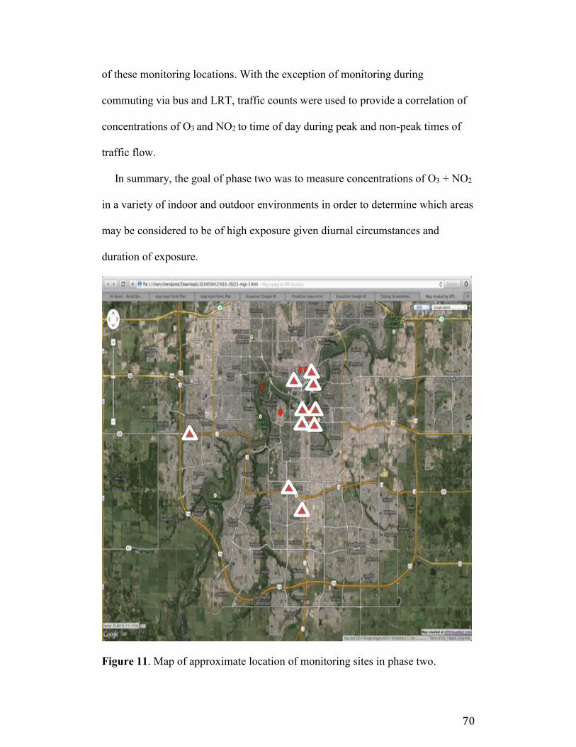
70
of these monitoring locations. With the exception of monitoring during
commuting via bus and LRT, traffic counts were used to provide a correlation of
concentrations of O3 and NO2 to time of day during peak and non-peak times of
traffic flow.
In summary, the goal of phase two was to measure concentrations of O3 + NO2
in a variety of indoor and outdoor environments in order to determine which areas
may be considered to be of high exposure given diurnal circumstances and
duration of exposure.
Figure 11. Map of approximate location of monitoring sites in phase two.

71
3.5 Indoor and Outdoor Residential Monitoring
The indoor and outdoor residential monitoring took place at an urban, intercity
home in Old Strathcona. The residential setting was situated within close
proximity to a major roadway, 99th Street and 88th Avenue, with high volumes of
vehicular traffic; densely populated with people and businesses close by.
Monitoring of the residential area was designed in order to compare indoor
concentrations to outdoor concentrations of O3 + NO2 in the study subject’s
residential area during the day. Sensors were placed inside the home and in the
backyard at this location. The data collected from these scenarios was used to
calculate ratios as a means of comparing concentrations of O3 + NO2 indoor to
those outdoor. Calculating concentration ratios of indoor versus outdoor enabled
for analysis and determination of which environment contained the highest
concentration during times of monitoring.
Cairclip 2 was placed indoors, attached to an inside wall, within range of the
kitchen and placed at breathing zone height, (Figure 12). A plastic zip tie was
used to attach the sensor to a wall hanging between the kitchen and dining areas,
free of obstruction to air flow. The outdoor sensor was placed in the middle of the
backyard of the home at the breathing zone height (Figure 13). The shelter that
was used for phase one was used to protect the sensors from rain, snow and wind.
Zip ties were used to secure the sensor in place (Figure 14).
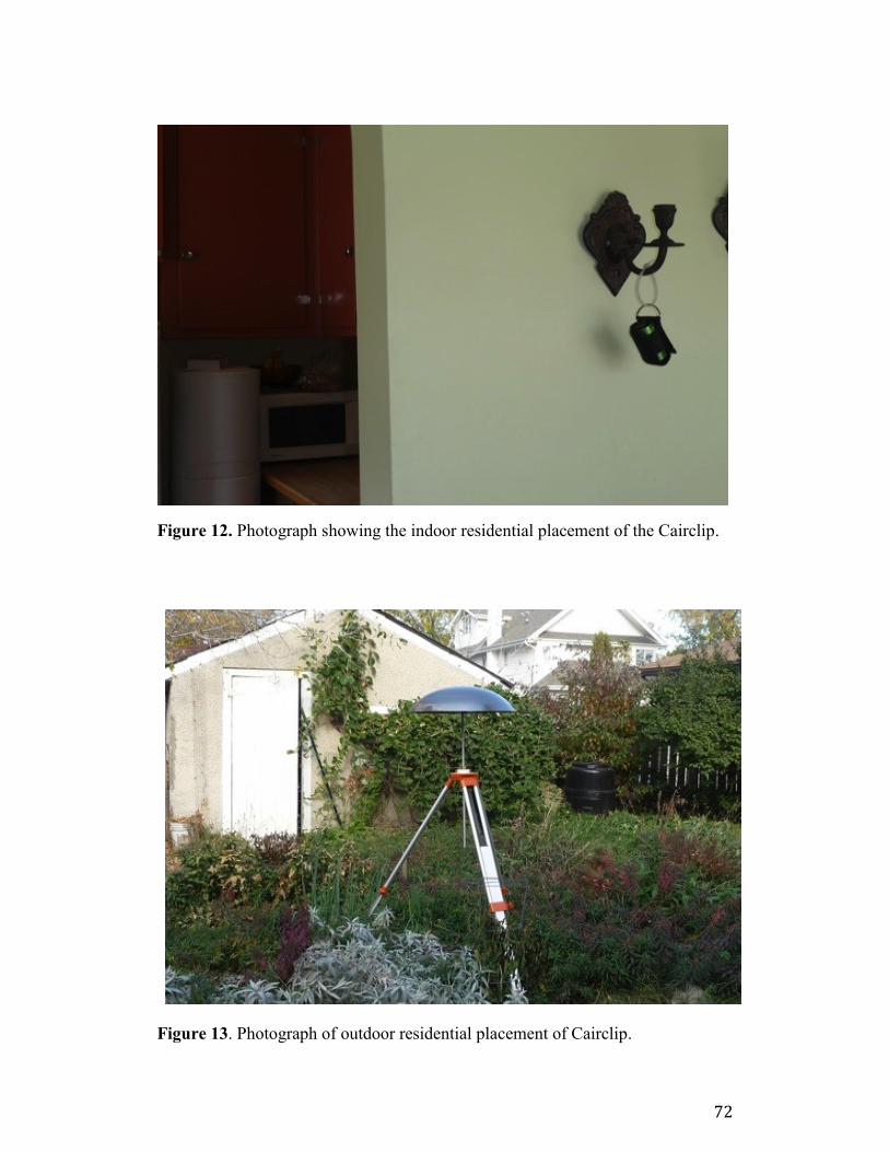
72
Figure 12. Photograph showing the indoor residential placement of the Cairclip.
Figure 13. Photograph of outdoor residential placement of Cairclip.
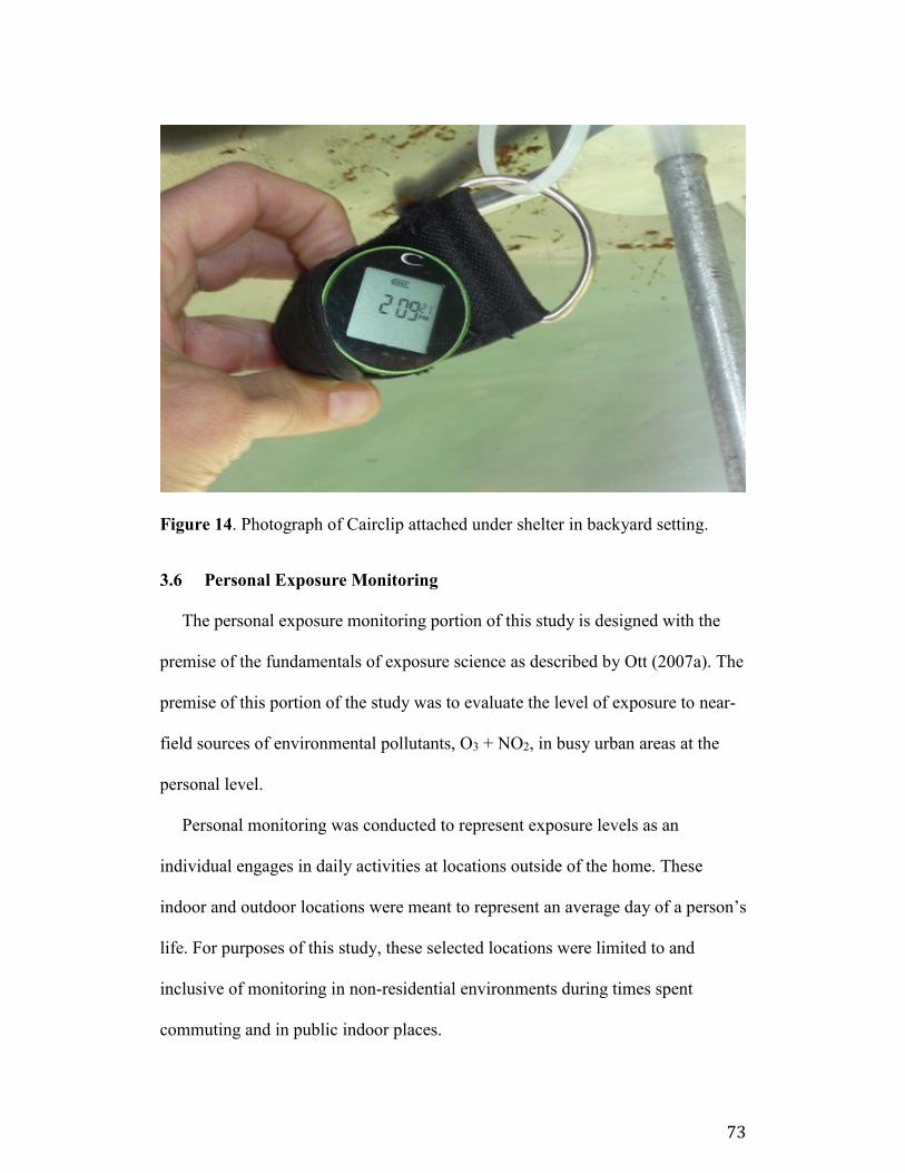
73
Figure 14. Photograph of Cairclip attached under shelter in backyard setting.
3.6 Personal Exposure Monitoring
The personal exposure monitoring portion of this study is designed with the
premise of the fundamentals of exposure science as described by Ott (2007a). The
premise of this portion of the study was to evaluate the level of exposure to near-
field sources of environmental pollutants, O3 + NO2, in busy urban areas at the
personal level.
Personal monitoring was conducted to represent exposure levels as an
individual engages in daily activities at locations outside of the home. These
indoor and outdoor locations were meant to represent an average day of a person’s
life. For purposes of this study, these selected locations were limited to and
inclusive of monitoring in non-residential environments during times spent
commuting and in public indoor places.

74
The personal monitor was worn within the range of the human breathing zone;
an area that lies with 10 inches in any direction of the mouth and nose (Ojima,
2012; Zhang & Lioy, 2002). Therefore, the monitor was attached to the upper arm
just below the shoulder with a Velcro strap for security during activities. Figures
15 and 16, demonstrate the placement and apparatus used to secure the sensor for
personal exposure monitoring. A time activity diary was used to supplement the
Cairclip sensors. The time activity diary was a tool used to provide for recording
of pertinent information relating to location, duration and any other circumstances
related to daily activities patterns of the individual (Ott, 2007a).
Figure 15. Photograph of Cairclip placement for personal monitoring.
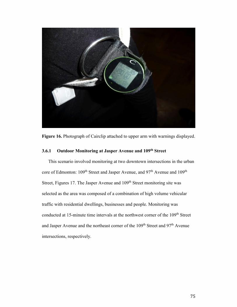
75
Figure 16. Photograph of Cairclip attached to upper arm with warnings displayed.
3.6.1 Outdoor Monitoring at Jasper Avenue and 109th Street
This scenario involved monitoring at two downtown intersections in the urban
core of Edmonton: 109th Street and Jasper Avenue, and 97th Avenue and 109th
Street, Figures 17. The Jasper Avenue and 109th Street monitoring site was
selected as the area was composed of a combination of high volume vehicular
traffic with residential dwellings, businesses and people. Monitoring was
conducted at 15-minute time intervals at the northwest corner of the 109th Street
and Jasper Avenue and the northeast corner of the 109th Street and 97th Avenue
intersections, respectively.
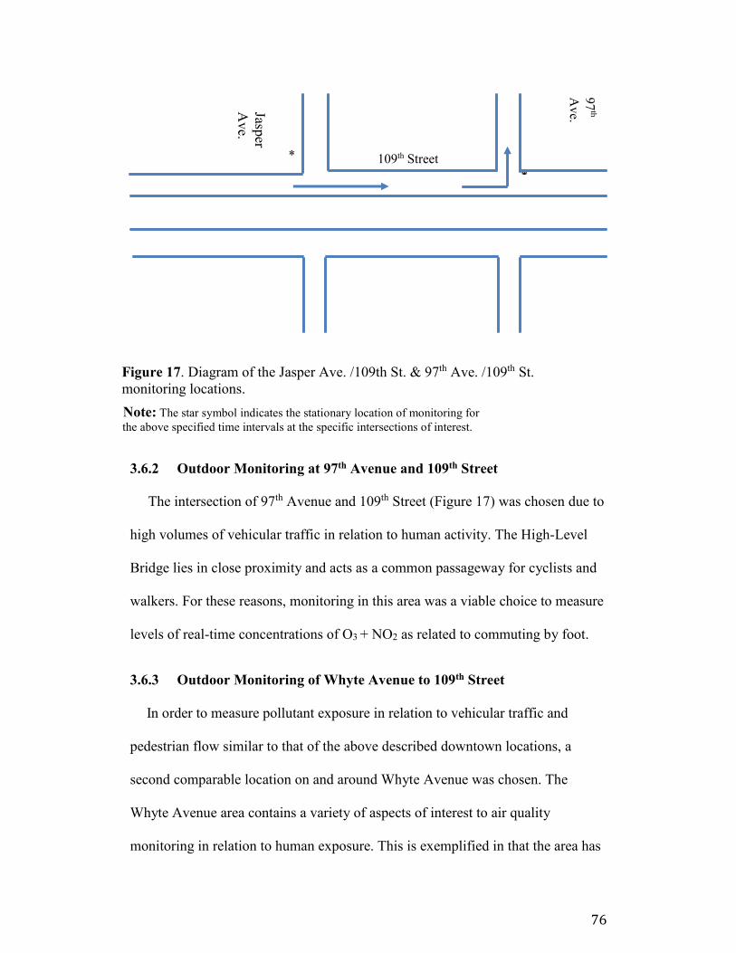
76
*
Note: The star symbol indicates the stationary location of monitoring for
the above specified time intervals at the specific intersections of interest.
3.6.2 Outdoor Monitoring at 97th Avenue and 109th Street
The intersection of 97th Avenue and 109th Street (Figure 17) was chosen due to
high volumes of vehicular traffic in relation to human activity. The High-Level
Bridge lies in close proximity and acts as a common passageway for cyclists and
walkers. For these reasons, monitoring in this area was a viable choice to measure
levels of real-time concentrations of O3 + NO2 as related to commuting by foot.
3.6.3 Outdoor Monitoring of Whyte Avenue to 109th Street
In order to measure pollutant exposure in relation to vehicular traffic and
pedestrian flow similar to that of the above described downtown locations, a
second comparable location on and around Whyte Avenue was chosen. The
Whyte Avenue area contains a variety of aspects of interest to air quality
monitoring in relation to human exposure. This is exemplified in that the area has
109th Street
*
Jasper
Ave.
97
th
Av
e.
Figure 17. Diagram of the Jasper Ave. /109th St. & 97th Ave. /109th St.
monitoring locations.
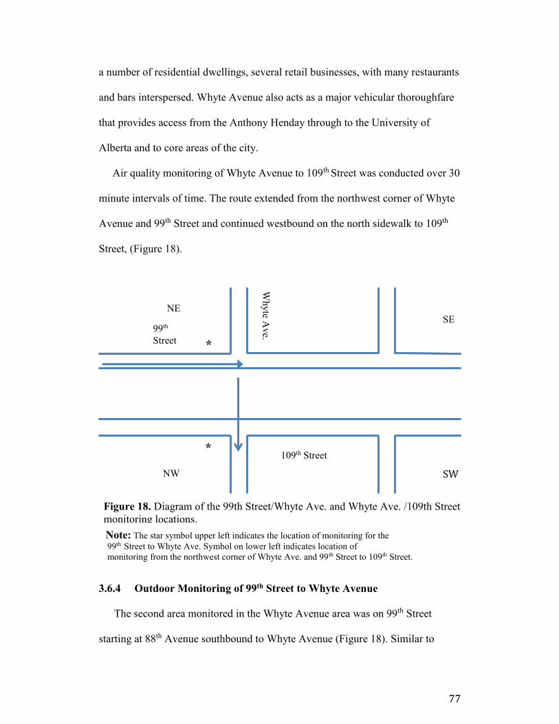
77
a number of residential dwellings, several retail businesses, with many restaurants
and bars interspersed. Whyte Avenue also acts as a major vehicular thoroughfare
that provides access from the Anthony Henday through to the University of
Alberta and to core areas of the city.
Air quality monitoring of Whyte Avenue to 109th Street was conducted over 30
minute intervals of time. The route extended from the northwest corner of Whyte
Avenue and 99th Street and continued westbound on the north sidewalk to 109th
Street, (Figure 18).
*
*
Note: The star symbol upper left indicates the location of monitoring for the
99th Street to Whyte Ave. Symbol on lower left indicates location of
monitoring from the northwest corner of Whyte Ave. and 99th Street to 109th Street.
3.6.4 Outdoor Monitoring of 99th Street to Whyte Avenue
The second area monitored in the Whyte Avenue area was on 99th Street
starting at 88th Avenue southbound to Whyte Avenue (Figure 18). Similar to
SE
NE
99th
Street
SW NW
109th Street
Whyte A
ve.
Figure 18. Diagram of the 99th Street/Whyte Ave. and Whyte Ave. /109th Street
monitoring locations.
Figure 18. Diagram of the 99th St./Whyte Ave & Whyte Ave./109th St. monitoring locations
locations.

78
Whyte Avenue, 99th Street acts as a major thoroughfare for vehicular traffic and
passes through areas of high density residential communities. As with the Whyte
Avenue to 109th Street route, monitoring was intended to capture personal
exposure to O3 and NO2 as a commuter travelling on foot in close proximity to
vehicular traffic.
The route encompassed travelling southbound on the east side of 99th Street
from 88th Avenue to Whyte Avenue, remaining at the intersection of Whyte
Avenue and 99th for a period of time and then returning by walking northbound on
the west side of 99th from Whyte Avenue to 89th Avenue. Monitoring times for
this exposure setting were also 30 minutes in duration.
3.7 Commuter Monitoring On Public Transportation
Commuter monitoring on public transportation involved traveling by bus and
by LRT. Monitoring in this scenario included travel time and wait times at
selected transit stations. The specific LRT and bus routes were selected to capture
routes that were used regularly by large volumes of commuters. Figure 19
illustrates the LRT and city bus route used for exposure monitoring during this
study.
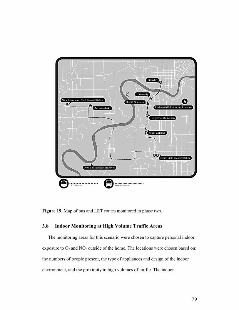
79
Figure 19. Map of bus and LRT routes monitored in phase two.
3.8 Indoor Monitoring at High Volume Traffic Areas
The monitoring areas for this scenario were chosen to capture personal indoor
exposure to O3 and NO2 outside of the home. The locations were chosen based on:
the numbers of people present, the type of appliances and design of the indoor
environment, and the proximity to high volumes of traffic. The indoor
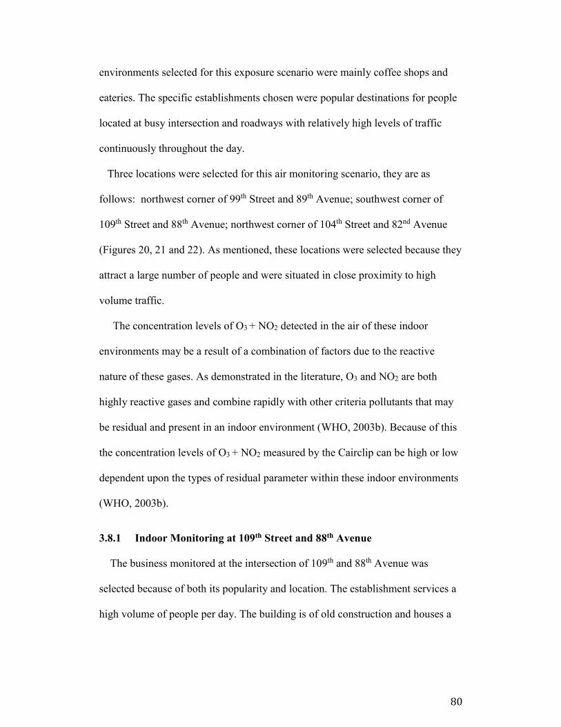
80
environments selected for this exposure scenario were mainly coffee shops and
eateries. The specific establishments chosen were popular destinations for people
located at busy intersection and roadways with relatively high levels of traffic
continuously throughout the day.
Three locations were selected for this air monitoring scenario, they are as
follows: northwest corner of 99th Street and 89th Avenue; southwest corner of
109th Street and 88th Avenue; northwest corner of 104th Street and 82nd Avenue
(Figures 20, 21 and 22). As mentioned, these locations were selected because they
attract a large number of people and were situated in close proximity to high
volume traffic.
The concentration levels of O3 + NO2 detected in the air of these indoor
environments may be a result of a combination of factors due to the reactive
nature of these gases. As demonstrated in the literature, O3 and NO2 are both
highly reactive gases and combine rapidly with other criteria pollutants that may
be residual and present in an indoor environment (WHO, 2003b). Because of this
the concentration levels of O3 + NO2 measured by the Cairclip can be high or low
dependent upon the types of residual parameter within these indoor environments
(WHO, 2003b).
3.8.1 Indoor Monitoring at 109th Street and 88th Avenue
The business monitored at the intersection of 109th and 88th Avenue was
selected because of both its popularity and location. The establishment services a
high volume of people per day. The building is of old construction and houses a
81
number of other business including a bike shop. The business is located close to a
residential area and immediately adjacent to a very busy intersection.
The indoor environment was located on the northwest corner of 109th Street
and 88th Avenue at the top of the High Level Bridge. The entrance to the
establishment is located on the 88th Avenue side (Figure 20). A small space
equipped with a commercial grade kitchen and cooking appliances, it acts as a
popular destination for people.
SW
109th Street
Figure 20. Diagram of the 109th St. & 88th Ave. indoor monitoring site.
Note: The star symbol indicates the stationary location of monitoring for the
above specified time intervals at the specific non-residential, indoor exposure
scenarios of interest.
3.8.2 Indoor Monitoring at 99th Street and 89th Avenue
The second indoor environment chosen for monitoring was in a restaurant
located on the northwest corner of 99th Street and 89th Avenue (Figure 21). The
front door of the establishment was situated approximately 1.5 meters from the
intersections of 99th Street and 89th Avenue. A secondary entrance was located
SE
NW
NE
*
88
th Ave.
Sask
. Dr.
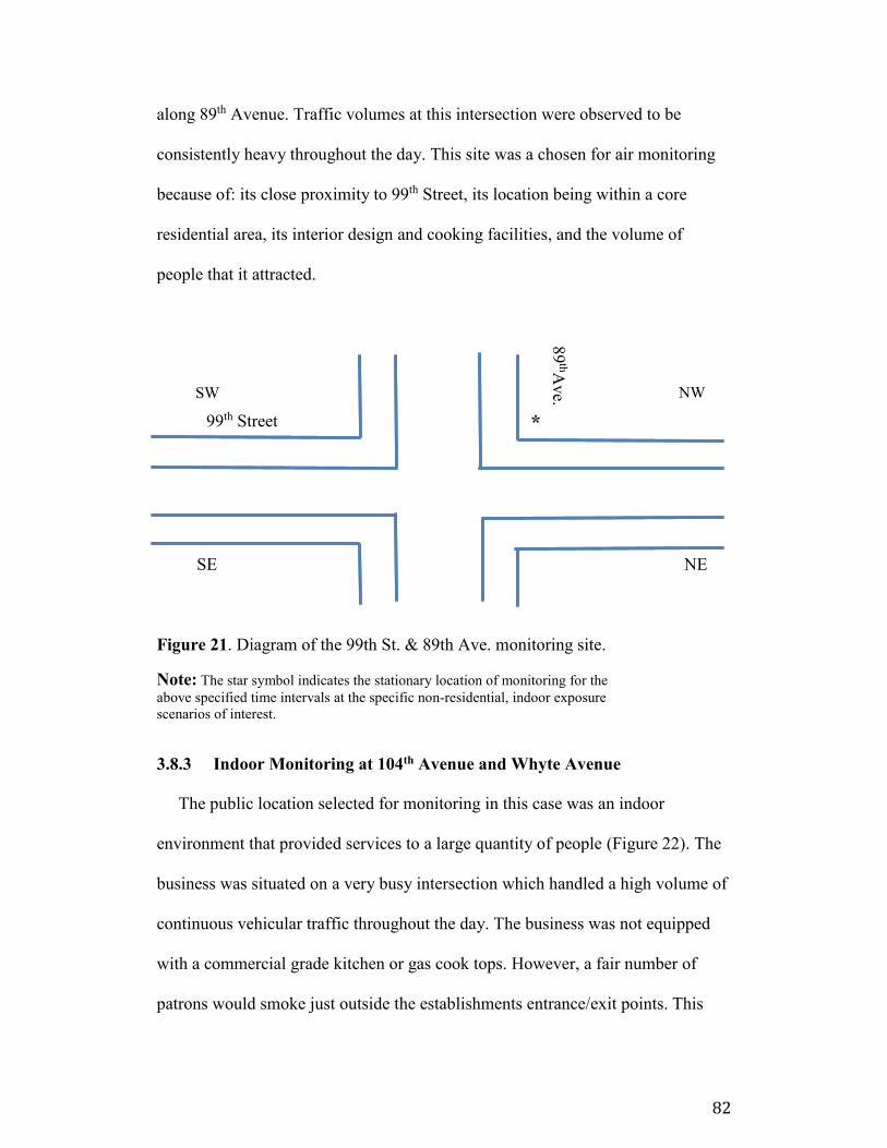
82
along 89th Avenue. Traffic volumes at this intersection were observed to be
consistently heavy throughout the day. This site was a chosen for air monitoring
because of: its close proximity to 99th Street, its location being within a core
residential area, its interior design and cooking facilities, and the volume of
people that it attracted.
SE NE
Figure 21. Diagram of the 99th St. & 89th Ave. monitoring site.
Note: The star symbol indicates the stationary location of monitoring for the
above specified time intervals at the specific non-residential, indoor exposure
scenarios of interest.
3.8.3 Indoor Monitoring at 104th Avenue and Whyte Avenue
The public location selected for monitoring in this case was an indoor
environment that provided services to a large quantity of people (Figure 22). The
business was situated on a very busy intersection which handled a high volume of
continuous vehicular traffic throughout the day. The business was not equipped
with a commercial grade kitchen or gas cook tops. However, a fair number of
patrons would smoke just outside the establishments entrance/exit points. This
*
NW SW
89
thAve.
99th Street
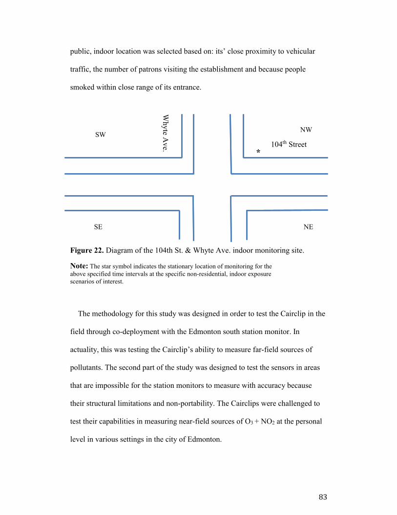
83
public, indoor location was selected based on: its’ close proximity to vehicular
traffic, the number of patrons visiting the establishment and because people
smoked within close range of its entrance.
SW
Figure 22. Diagram of the 104th St. & Whyte Ave. indoor monitoring site.
Note: The star symbol indicates the stationary location of monitoring for the
above specified time intervals at the specific non-residential, indoor exposure
scenarios of interest.
The methodology for this study was designed in order to test the Cairclip in the
field through co-deployment with the Edmonton south station monitor. In
actuality, this was testing the Cairclip’s ability to measure far-field sources of
pollutants. The second part of the study was designed to test the sensors in areas
that are impossible for the station monitors to measure with accuracy because
their structural limitations and non-portability. The Cairclips were challenged to
test their capabilities in measuring near-field sources of O3 + NO2 at the personal
level in various settings in the city of Edmonton.
SE
NW
NE
* 104th Street
Whyte A
ve.
84
4 RESULTS AND DISCUSSION
4.1 Phase One Replicate Monitoring and Field Precision of Cairclips
According to the manufacturer’s technical data sheet found in Appendix A, the
degree of uncertainty of the sensors has been established as < 30% (Cairpol,
2014). The Cairpol company has acquired this value of uncertainty for the
Cairclip O3/NO2 sensor based on the DQO set by the European Commission in
2008 (European Commission, 2008b). This value encompasses uncertainty
percentages defined for various measurements of which include fixed
measurements and indicative measurements. The uncertainty value of < 30% is
expressed at a 95% confidence interval of the individual measurements averaged
over the period of the limit value for NO2 and the target value for O3 (European
Commission, 2008b).
Tables 4 to 15, provide a summary of the quantitative parameter precision
analysis and the linear regression results of three data set groupings; including
screened data, data with visual outliers removed and remaining data after all
points beyond ±2SD were removed. The data analyzed here was collected during
active monitoring of O3 and NO2 when Cairclip sensors were deployed on location
at the NAPS Edmonton south station. The summarized precision findings of
paired Cairclips for the time averaged concentrations of one hour, 30 and 15
minute ranged from: ±11 to 34%; ±12 to 39%; and ±14 to 37%.
The precision data was compared at three time weighted concentration
intervals of one hour, 30 and 15 minute time frames. For the purposes of this
document, the one hour precision results are displayed for each pairing of the
85
Cairclip sensors 1 to 4 in the following text. Both the 30 and 15 minute time
weighted concentration precision results are provided in Appendix C. In each
table, group one are all screened data, group two are data sets with visual outliers
removed and group three are data with outliers removed based on ±2 SD from the
mean value. The acronym CC is used in all the precision tables to represent the
Cairclip sensor while SM represents the Edmonton South station monitor.
Results of the linear regression are also displayed in tables and allow
comparison of the data before and after outlying data points were removed. All
values in the linear regression tables are rounded to two significant values. The
linear regression graphs and tables for one hour time weighted precision results
are discussed in the following text. Graphs and tables of linear regression results
for 30 and 15 minute time weighted averages are provided in Appendix C.
Figure 23 is provided as an example showing all the paired screened precision
data for Cairclip 1 vs. Cairclip 2 with lines showing ±2SD in relation to the fitted
linear regression line. Although, this relationship is only presented in the text in
Figure 23, the same quantitative process was applied to all other precision data
sets.
4.1.1 Precision Results Cairclip 1 to Cairclip 2 A summary of the precision results for paired sensors, Cairclip 1 and 2 is
provided in Table 4. For the paired Cairclips 1 and 2, the percent relative standard
deviation (%RSD) was 34% (n=100), 20% (n=94) and 20% (n=94) for group 1, 2
and 3, respectively. The %RSD decreased from 34% (all screened data) to 20%
when visual outliers were removed; the %RSD remained the same after the

86
m±2SD outlier test was applied as all points remained within the 95%; no
additional points were considered to be outliers.
During phase one, the mean ambient concentration value detected by Cairclip
1 ranged from 17 to 18 ppb, a value below the limit of detection (LOD) of 20 ppb
as set by the manufacturer. Cairclip 2 measured a mean concentration of 20 ppb,
and concurrent with the LOD.
Table 4. Field precision parameter results of Cairclip 1 to Cairclip 2.
Parameters for
Precision Analysis
Group 1
(all screened
data)
Group 2
(screened data
with visual outliers
removed)
Group 3
(screened data with
outliers removed
beyond m±2SD)
CC1 CC2 CC1 CC2 CC1 CC2
N 100 94 94
Mean (ppb) 17.3 20 18 20 18 20
Median (ppb) 17 19 17 19 17 19
Mode (ppb) 17 26 17 26 17 26
Min (ppb) 4 5 4 5 4 5
Max (ppb) 32 40 32 40 32 40
%RSD 34% 20% 20%
The graph of the precision data paired Cairlclips 1 to 2 is shown in Figure 23,
followed by a summary of the linear regression results for the one hour averaged
concentrations of O3 + NO2 (Table 5). As mentioned, Figure 23 represents all
screened data (group 1) plotted in relation to lines showing data exclusion once the ±2SD
outliers test was applied (group 3). A one to one line is shown to illustrate an ideal slope
as well as he best fit linear regression line is shown on the graphs as applied to the
remaining data after the ±2SD testing (group 3). This graph is provided in this fashion in
order to illustrate which paired data points were quantitatively removed for all precision
data of paired Cairclips. This detailed information is provided exclusively in this
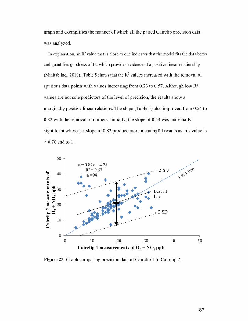
87
graph and exemplifies the manner of which all the paired Cairclip precision data
was analyzed.
In explanation, an R2 value that is close to one indicates that the model fits the data better
and quantifies goodness of fit, which provides evidence of a positive linear relationship
(Minitab Inc., 2010). Table 5 shows that the R2 values increased with the removal of
spurious data points with values increasing from 0.23 to 0.57. Although low R2
values are not sole predictors of the level of precision, the results show a
marginally positive linear relations. The slope (Table 5) also improved from 0.54 to
0.82 with the removal of outliers. Initially, the slope of 0.54 was marginally
significant whereas a slope of 0.82 produce more meaningful results as this value is
> 0.70 and to 1.
Figure 23. Graph comparing precision data of Cairclip 1 to Cairclip 2.
0
10
20
30
40
50
0 10 20 30 40 50
Cair
clip
2 m
easu
rem
ents
of
O3
+ N
O2
pp
b
Cairclip 1 measurements of O3 + NO2 ppb
+ 2 SD
- 2 SD
y = 0.82x + 4.78
R2 = 0.57
n =94
Best fit
line
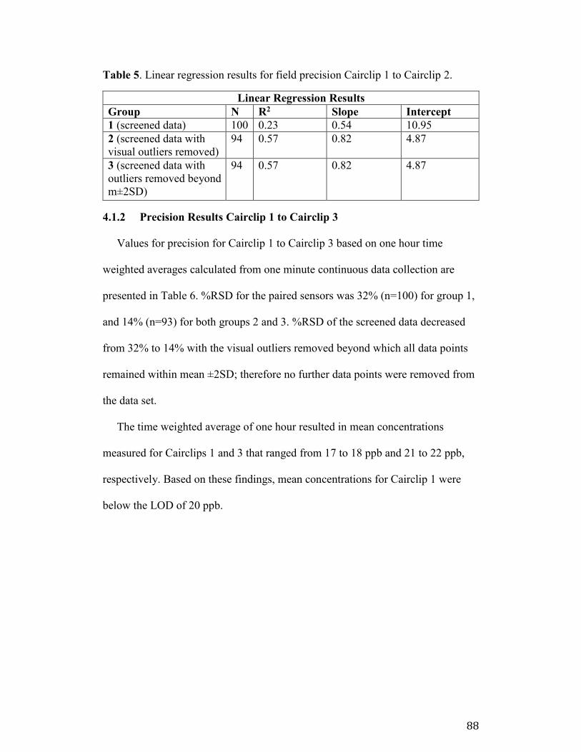
88
Table 5. Linear regression results for field precision Cairclip 1 to Cairclip 2.
Linear Regression Results
Group N R2 Slope Intercept
1 (screened data) 100 0.23 0.54 10.95
2 (screened data with
visual outliers removed)
94 0.57 0.82 4.87
3 (screened data with
outliers removed beyond
m±2SD)
94 0.57 0.82 4.87
4.1.2 Precision Results Cairclip 1 to Cairclip 3
Values for precision for Cairclip 1 to Cairclip 3 based on one hour time
weighted averages calculated from one minute continuous data collection are
presented in Table 6. %RSD for the paired sensors was 32% (n=100) for group 1,
and 14% (n=93) for both groups 2 and 3. %RSD of the screened data decreased
from 32% to 14% with the visual outliers removed beyond which all data points
remained within mean ±2SD; therefore no further data points were removed from
the data set.
The time weighted average of one hour resulted in mean concentrations
measured for Cairclips 1 and 3 that ranged from 17 to 18 ppb and 21 to 22 ppb,
respectively. Based on these findings, mean concentrations for Cairclip 1 were
below the LOD of 20 ppb.
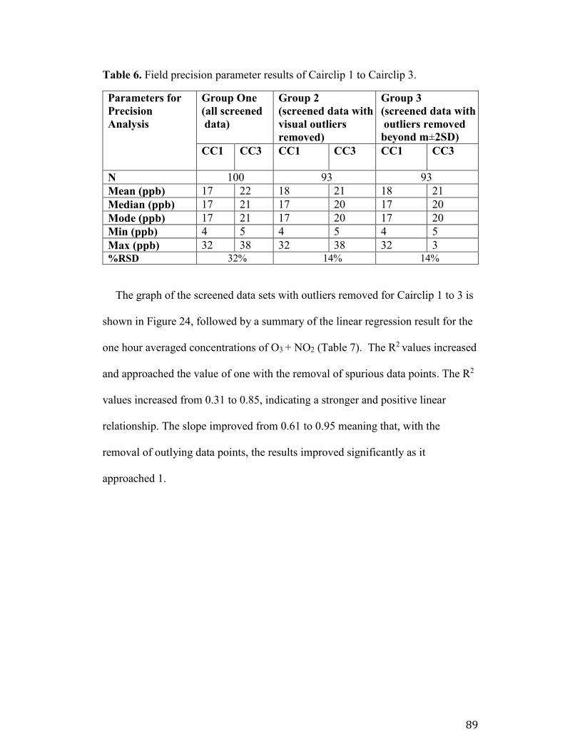
89
Table 6. Field precision parameter results of Cairclip 1 to Cairclip 3.
Parameters for
Precision
Analysis
Group One
(all screened
data)
Group 2
(screened data with
visual outliers
removed)
Group 3
(screened data with
outliers removed
beyond m±2SD)
CC1 CC3 CC1
CC3 CC1 CC3
N 100 93 93
Mean (ppb) 17 22 18 21 18 21
Median (ppb) 17 21 17 20 17 20
Mode (ppb) 17 21 17 20 17 20
Min (ppb) 4 5 4 5 4 5
Max (ppb) 32 38 32 38 32 3
%RSD 32% 14% 14%
The graph of the screened data sets with outliers removed for Cairclip 1 to 3 is
shown in Figure 24, followed by a summary of the linear regression result for the
one hour averaged concentrations of O3 + NO2 (Table 7). The R2 values increased
and approached the value of one with the removal of spurious data points. The R2
values increased from 0.31 to 0.85, indicating a stronger and positive linear
relationship. The slope improved from 0.61 to 0.95 meaning that, with the
removal of outlying data points, the results improved significantly as it
approached 1.
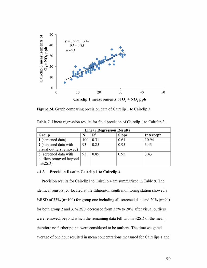
90
Figure 24. Graph comparing precision data of Cairclip 1 to Cairclip 3.
Table 7. Linear regression results for field precision of Cairclip 1 to Cairclip 3.
Linear Regression Results
Group N R2 Slope Intercept
1 (screened data) 100 0.31 0.61 10.94
2 (screened data with
visual outliers removed)
93 0.85 0.95 3.43
3 (screened data with
outliers removed beyond
m±2SD)
93 0.85 0.95 3.43
4.1.3 Precision Results Cairclip 1 to Cairclip 4
Precision results for Cairclip1 to Cairclip 4 are summarized in Table 9. The
identical sensors, co-located at the Edmonton south monitoring station showed a
%RSD of 33% (n=100) for group one including all screened data and 20% (n=94)
for both group 2 and 3. %RSD decreased from 33% to 20% after visual outliers
were removed, beyond which the remaining data fell within ±2SD of the mean;
therefore no further points were considered to be outliers. The time weighted
average of one hour resulted in mean concentrations measured for Cairclips 1 and
y = 0.95x + 3.42
R² = 0.85
0
10
20
30
40
50
0 10 20 30 40 50
Cair
clip
3 m
easu
rem
ents
of
O3
+ N
O2
pp
b
Cairclip 1 measurements of O3 + NO2 ppb
n = 93
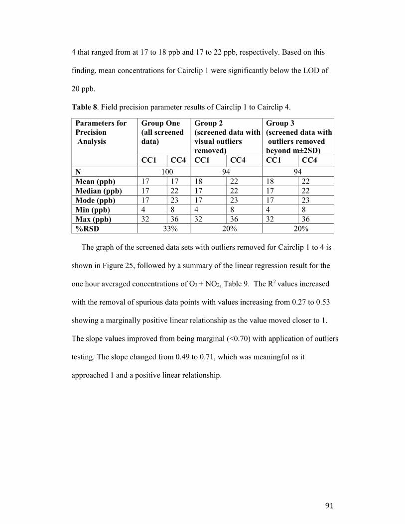
91
4 that ranged from at 17 to 18 ppb and 17 to 22 ppb, respectively. Based on this
finding, mean concentrations for Cairclip 1 were significantly below the LOD of
20 ppb.
Table 8. Field precision parameter results of Cairclip 1 to Cairclip 4.
Parameters for
Precision
Analysis
Group One
(all screened
data)
Group 2
(screened data with
visual outliers
removed)
Group 3
(screened data with
outliers removed
beyond m±2SD)
CC1 CC4 CC1 CC4 CC1 CC4
N 100 94 94
Mean (ppb) 17 17 18 22 18 22
Median (ppb) 17 22 17 22 17 22
Mode (ppb) 17 23 17 23 17 23
Min (ppb) 4 8 4 8 4 8
Max (ppb) 32 36 32 36 32 36
%RSD 33% 20% 20%
The graph of the screened data sets with outliers removed for Cairclip 1 to 4 is
shown in Figure 25, followed by a summary of the linear regression result for the
one hour averaged concentrations of O3 + NO2, Table 9. The R2 values increased
with the removal of spurious data points with values increasing from 0.27 to 0.53
showing a marginally positive linear relationship as the value moved closer to 1.
The slope values improved from being marginal (<0.70) with application of outliers
testing. The slope changed from 0.49 to 0.71, which was meaningful as it
approached 1 and a positive linear relationship.
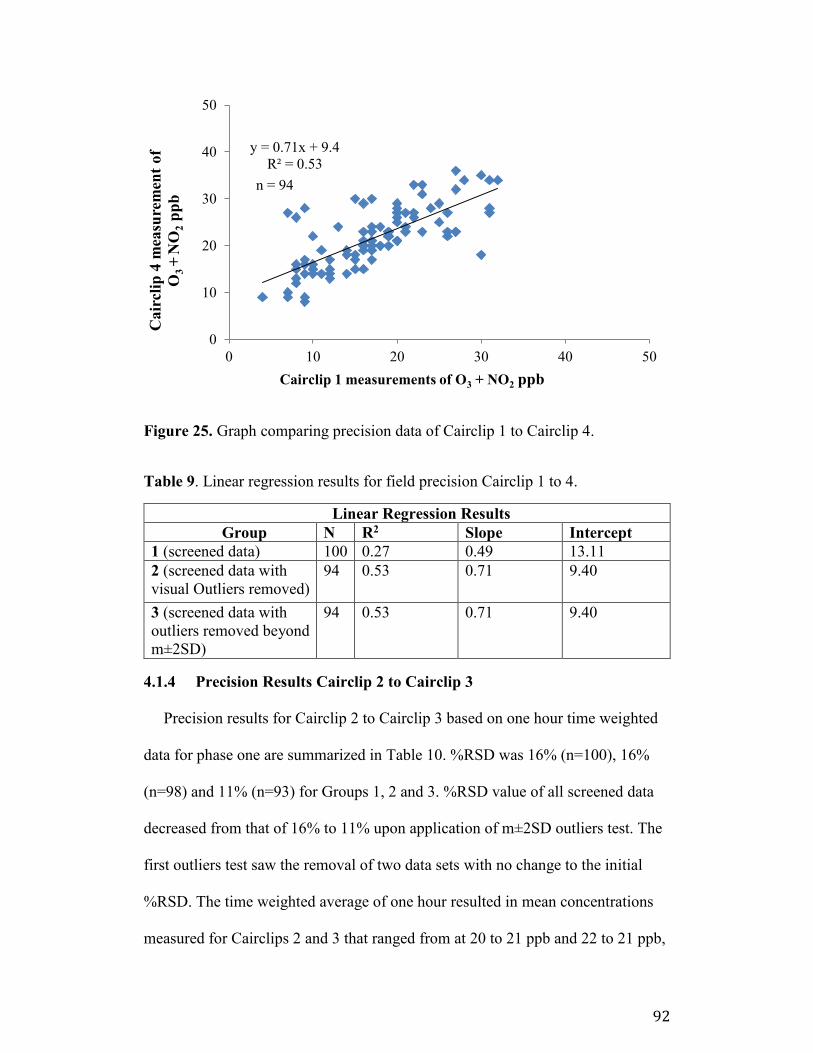
92
Figure 25. Graph comparing precision data of Cairclip 1 to Cairclip 4.
Table 9. Linear regression results for field precision Cairclip 1 to 4.
Linear Regression Results
Group N R2 Slope Intercept
1 (screened data) 100 0.27 0.49 13.11
2 (screened data with
visual Outliers removed)
94 0.53 0.71 9.40
3 (screened data with
outliers removed beyond
m±2SD)
94 0.53 0.71 9.40
4.1.4 Precision Results Cairclip 2 to Cairclip 3
Precision results for Cairclip 2 to Cairclip 3 based on one hour time weighted
data for phase one are summarized in Table 10. %RSD was 16% (n=100), 16%
(n=98) and 11% (n=93) for Groups 1, 2 and 3. %RSD value of all screened data
decreased from that of 16% to 11% upon application of m±2SD outliers test. The
first outliers test saw the removal of two data sets with no change to the initial
%RSD. The time weighted average of one hour resulted in mean concentrations
measured for Cairclips 2 and 3 that ranged from at 20 to 21 ppb and 22 to 21 ppb,
y = 0.71x + 9.4
R² = 0.53
0
10
20
30
40
50
0 10 20 30 40 50
Ca
ircl
ip 4
mea
sure
men
t o
f
O3
+N
O2
pp
b
Cairclip 1 measurements of O3 + NO2 ppb
n = 94
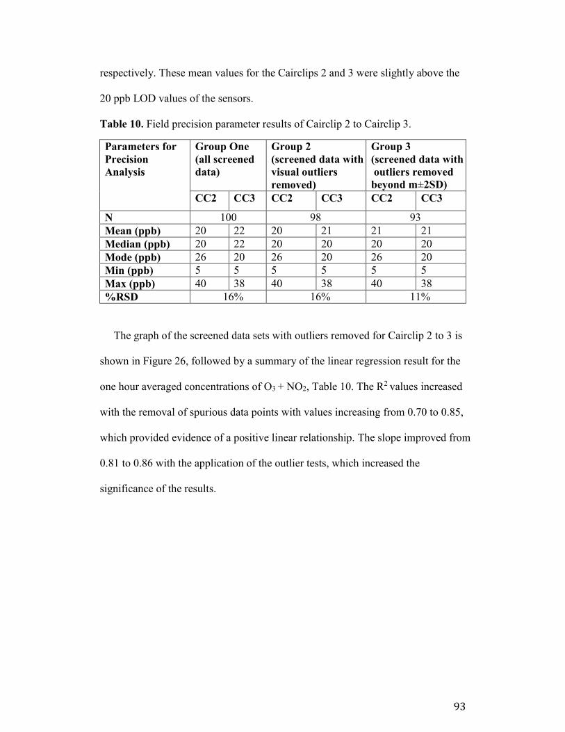
93
respectively. These mean values for the Cairclips 2 and 3 were slightly above the
20 ppb LOD values of the sensors.
Table 10. Field precision parameter results of Cairclip 2 to Cairclip 3.
Parameters for
Precision
Analysis
Group One
(all screened
data)
Group 2
(screened data with
visual outliers
removed)
Group 3
(screened data with
outliers removed
beyond m±2SD)
CC2 CC3 CC2 CC3 CC2 CC3
N 100 98 93
Mean (ppb) 20 22 20 21 21 21
Median (ppb) 20 22 20 20 20 20
Mode (ppb) 26 20 26 20 26 20
Min (ppb) 5 5 5 5 5 5
Max (ppb) 40 38 40 38 40 38
%RSD 16% 16% 11%
The graph of the screened data sets with outliers removed for Cairclip 2 to 3 is
shown in Figure 26, followed by a summary of the linear regression result for the
one hour averaged concentrations of O3 + NO2, Table 10. The R2 values increased
with the removal of spurious data points with values increasing from 0.70 to 0.85,
which provided evidence of a positive linear relationship. The slope improved from
0.81 to 0.86 with the application of the outlier tests, which increased the
significance of the results.
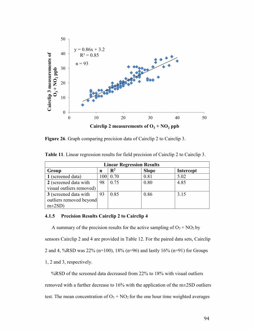
94
Figure 26. Graph comparing precision data of Cairclip 2 to Cairclip 3.
Table 11. Linear regression results for field precision of Cairclip 2 to Cairclip 3.
Linear Regression Results
Group n R2 Slope Intercept
1 (screened data) 100 0.70 0.81 5.02
2 (screened data with
visual outliers removed)
98 0.75 0.80 4.85
3 (screened data with
outliers removed beyond
m±2SD)
93 0.85 0.86 3.15
4.1.5 Precision Results Cairclip 2 to Cairclip 4
A summary of the precision results for the active sampling of O3 + NO2 by
sensors Cairclip 2 and 4 are provided in Table 12. For the paired data sets, Cairclip
2 and 4, %RSD was 22% (n=100), 18% (n=96) and lastly 16% (n=91) for Groups
1, 2 and 3, respectively.
%RSD of the screened data decreased from 22% to 18% with visual outliers
removed with a further decrease to 16% with the application of the m±2SD outliers
test. The mean concentration of O3 + NO2 for the one hour time weighted averages
y = 0.86x + 3.2
R² = 0.85
0
10
20
30
40
50
0 10 20 30 40 50
Cair
clip
3 m
easu
rem
ents
of
O3
+ N
O2
pp
b
Cairclip 2 measurements of O3 + NO2 ppb
n = 93
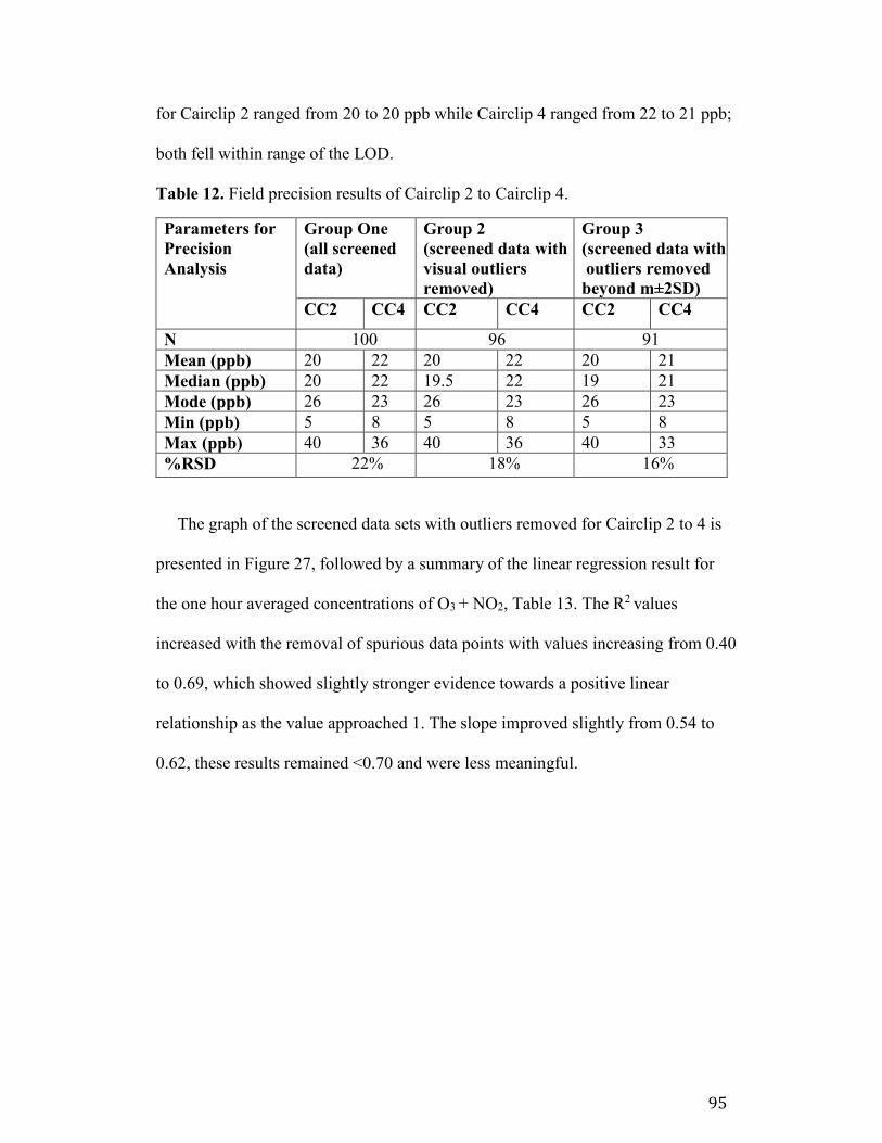
95
for Cairclip 2 ranged from 20 to 20 ppb while Cairclip 4 ranged from 22 to 21 ppb;
both fell within range of the LOD.
Table 12. Field precision results of Cairclip 2 to Cairclip 4.
Parameters for
Precision
Analysis
Group One
(all screened
data)
Group 2
(screened data with
visual outliers
removed)
Group 3
(screened data with
outliers removed
beyond m±2SD)
CC2 CC4 CC2 CC4 CC2 CC4
N 100 96 91
Mean (ppb) 20 22 20 22 20 21
Median (ppb) 20 22 19.5 22 19 21
Mode (ppb) 26 23 26 23 26 23
Min (ppb) 5 8 5 8 5 8
Max (ppb) 40 36 40 36 40 33
%RSD 22% 18% 16%
The graph of the screened data sets with outliers removed for Cairclip 2 to 4 is
presented in Figure 27, followed by a summary of the linear regression result for
the one hour averaged concentrations of O3 + NO2, Table 13. The R2 values
increased with the removal of spurious data points with values increasing from 0.40
to 0.69, which showed slightly stronger evidence towards a positive linear
relationship as the value approached 1. The slope improved slightly from 0.54 to
0.62, these results remained <0.70 and were less meaningful.
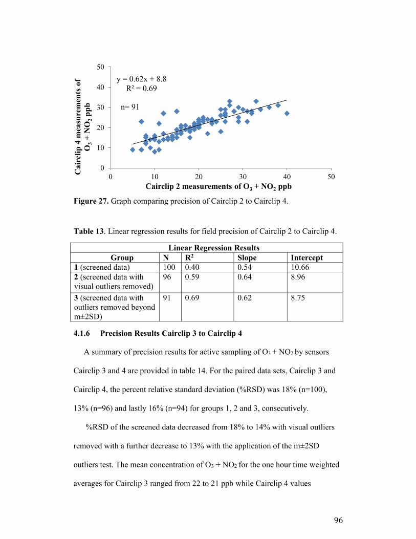
96
Figure 27. Graph comparing precision of Cairclip 2 to Cairclip 4.
Table 13. Linear regression results for field precision of Cairclip 2 to Cairclip 4.
Linear Regression Results
Group N R2 Slope Intercept
1 (screened data) 100 0.40 0.54 10.66
2 (screened data with
visual outliers removed)
96 0.59 0.64 8.96
3 (screened data with
outliers removed beyond
m±2SD)
91 0.69 0.62 8.75
4.1.6 Precision Results Cairclip 3 to Cairclip 4
A summary of precision results for active sampling of O3 + NO2 by sensors
Cairclip 3 and 4 are provided in table 14. For the paired data sets, Cairclip 3 and
Cairclip 4, the percent relative standard deviation (%RSD) was 18% (n=100),
13% (n=96) and lastly 16% (n=94) for groups 1, 2 and 3, consecutively.
%RSD of the screened data decreased from 18% to 14% with visual outliers
removed with a further decrease to 13% with the application of the m±2SD
outliers test. The mean concentration of O3 + NO2 for the one hour time weighted
averages for Cairclip 3 ranged from 22 to 21 ppb while Cairclip 4 values
y = 0.62x + 8.8
R² = 0.69
0
10
20
30
40
50
0 10 20 30 40 50
Cair
clip
4 m
easu
rem
ents
of
O3
+ N
O2
pp
b
Cairclip 2 measurements of O3 + NO2 ppb
n= 91
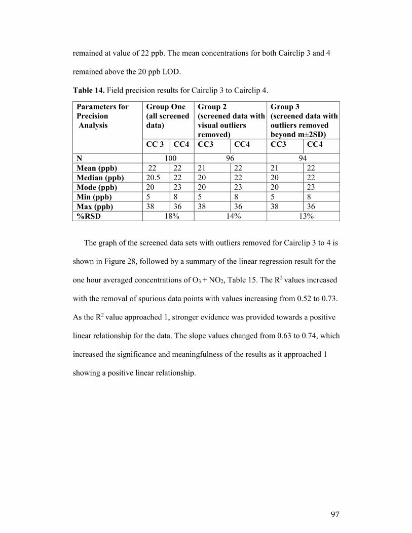
97
remained at value of 22 ppb. The mean concentrations for both Cairclip 3 and 4
remained above the 20 ppb LOD.
Table 14. Field precision results for Cairclip 3 to Cairclip 4.
Parameters for
Precision
Analysis
Group One
(all screened
data)
Group 2
(screened data with
visual outliers
removed)
Group 3
(screened data with
outliers removed
beyond m±2SD)
CC 3 CC4 CC3 CC4 CC3 CC4
N 100 96 94
Mean (ppb) 22 22 21 22 21 22
Median (ppb) 20.5 22 20 22 20 22
Mode (ppb) 20 23 20 23 20 23
Min (ppb) 5 8 5 8 5 8
Max (ppb) 38 36 38 36 38 36
%RSD 18% 14% 13%
The graph of the screened data sets with outliers removed for Cairclip 3 to 4 is
shown in Figure 28, followed by a summary of the linear regression result for the
one hour averaged concentrations of O3 + NO2, Table 15. The R2 values increased
with the removal of spurious data points with values increasing from 0.52 to 0.73.
As the R2 value approached 1, stronger evidence was provided towards a positive
linear relationship for the data. The slope values changed from 0.63 to 0.74, which
increased the significance and meaningfulness of the results as it approached 1
showing a positive linear relationship.
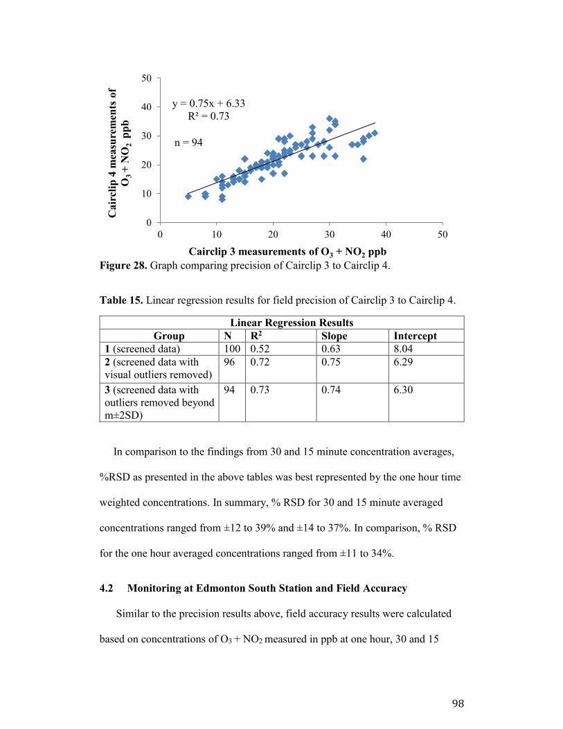
98
Figure 28. Graph comparing precision of Cairclip 3 to Cairclip 4.
Table 15. Linear regression results for field precision of Cairclip 3 to Cairclip 4.
Linear Regression Results
Group N R2 Slope Intercept
1 (screened data) 100 0.52 0.63 8.04
2 (screened data with
visual outliers removed)
96 0.72 0.75 6.29
3 (screened data with
outliers removed beyond
m±2SD)
94 0.73 0.74 6.30
In comparison to the findings from 30 and 15 minute concentration averages,
%RSD as presented in the above tables was best represented by the one hour time
weighted concentrations. In summary, % RSD for 30 and 15 minute averaged
concentrations ranged from ±12 to 39% and ±14 to 37%. In comparison, % RSD
for the one hour averaged concentrations ranged from ±11 to 34%.
4.2 Monitoring at Edmonton South Station and Field Accuracy
Similar to the precision results above, field accuracy results were calculated
based on concentrations of O3 + NO2 measured in ppb at one hour, 30 and 15
y = 0.75x + 6.33
R² = 0.73
0
10
20
30
40
50
0 10 20 30 40 50
Cair
clip
4 m
easu
rem
ents
of
O3
+ N
O2
p
pb
Cairclip 3 measurements of O3 + NO2 ppb
n = 94
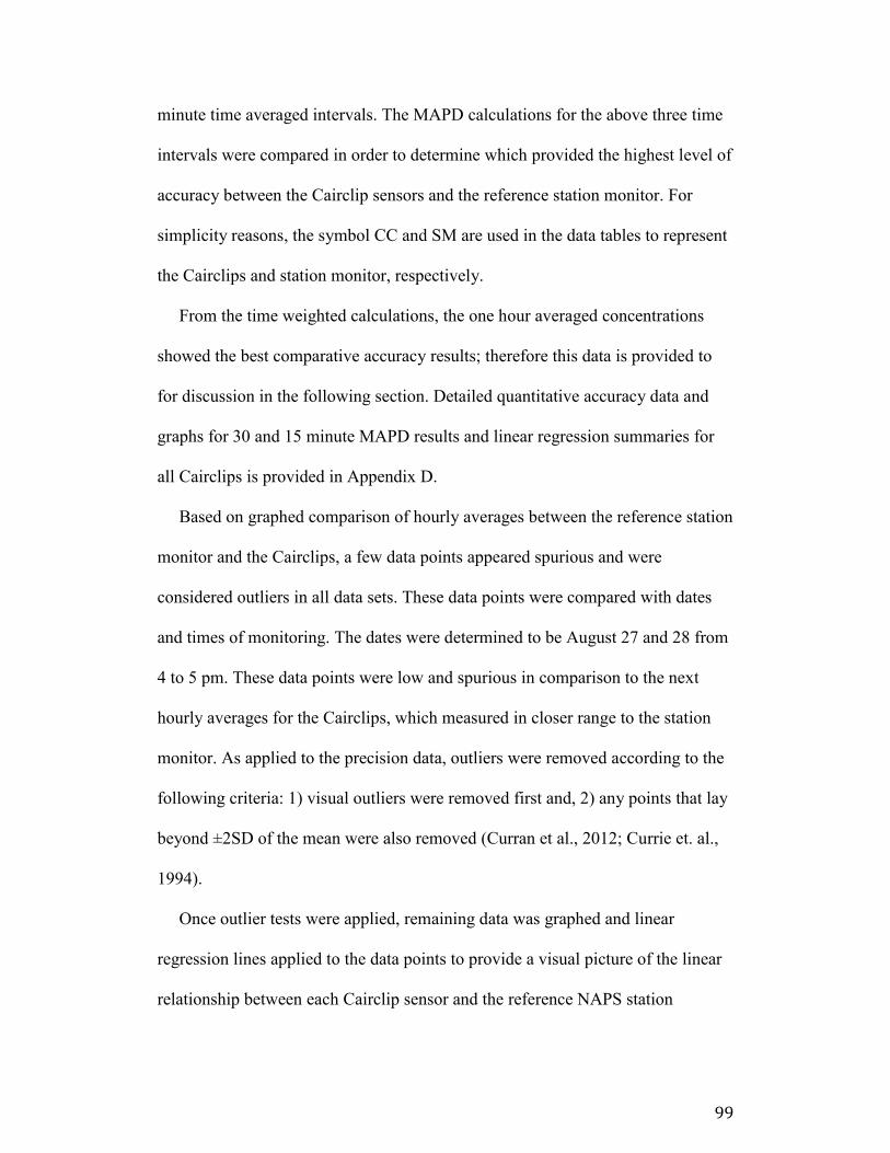
99
minute time averaged intervals. The MAPD calculations for the above three time
intervals were compared in order to determine which provided the highest level of
accuracy between the Cairclip sensors and the reference station monitor. For
simplicity reasons, the symbol CC and SM are used in the data tables to represent
the Cairclips and station monitor, respectively.
From the time weighted calculations, the one hour averaged concentrations
showed the best comparative accuracy results; therefore this data is provided to
for discussion in the following section. Detailed quantitative accuracy data and
graphs for 30 and 15 minute MAPD results and linear regression summaries for
all Cairclips is provided in Appendix D.
Based on graphed comparison of hourly averages between the reference station
monitor and the Cairclips, a few data points appeared spurious and were
considered outliers in all data sets. These data points were compared with dates
and times of monitoring. The dates were determined to be August 27 and 28 from
4 to 5 pm. These data points were low and spurious in comparison to the next
hourly averages for the Cairclips, which measured in closer range to the station
monitor. As applied to the precision data, outliers were removed according to the
following criteria: 1) visual outliers were removed first and, 2) any points that lay
beyond ±2SD of the mean were also removed (Curran et al., 2012; Currie et. al.,
1994).
Once outlier tests were applied, remaining data was graphed and linear
regression lines applied to the data points to provide a visual picture of the linear
relationship between each Cairclip sensor and the reference NAPS station

100
monitor. The best fit linear regression line graph is provided for each data set
followed by a table summarizing the results of three classifications of data as
follows: all screened data, data with visual outliers removed and remaining data
after the SD outliers test was applied.
The data sets used for the following graphs are representative of group 3 with
±2SD outlier test applied for one hour averaged concentrations of the Cairclip
sensor vs station monitor for monitoring from July to November, 2013.
Phase one findings are highlighted in Figure 29, the graph provides an
overview showing the performance of Cairclips 1, 2, 3 and 4 in relation to
measurements recorded by the station monitor based on hourly averaged
concentrations of O3 + NO2. This graph was designed to provide a general idea of
how well the Cairclips performed in relation with the reference or fixed site
monitor. In most cases, for the one hour average, the station monitor
concentration measurements for O3 + NO2 were higher than that of the Cairclip
sensor. This may be explained in that the Cairclip sensor lacks sensitivity in
environments where concentrations of O3 and NO2 are low such as that in the city
of Edmonton, Alberta.
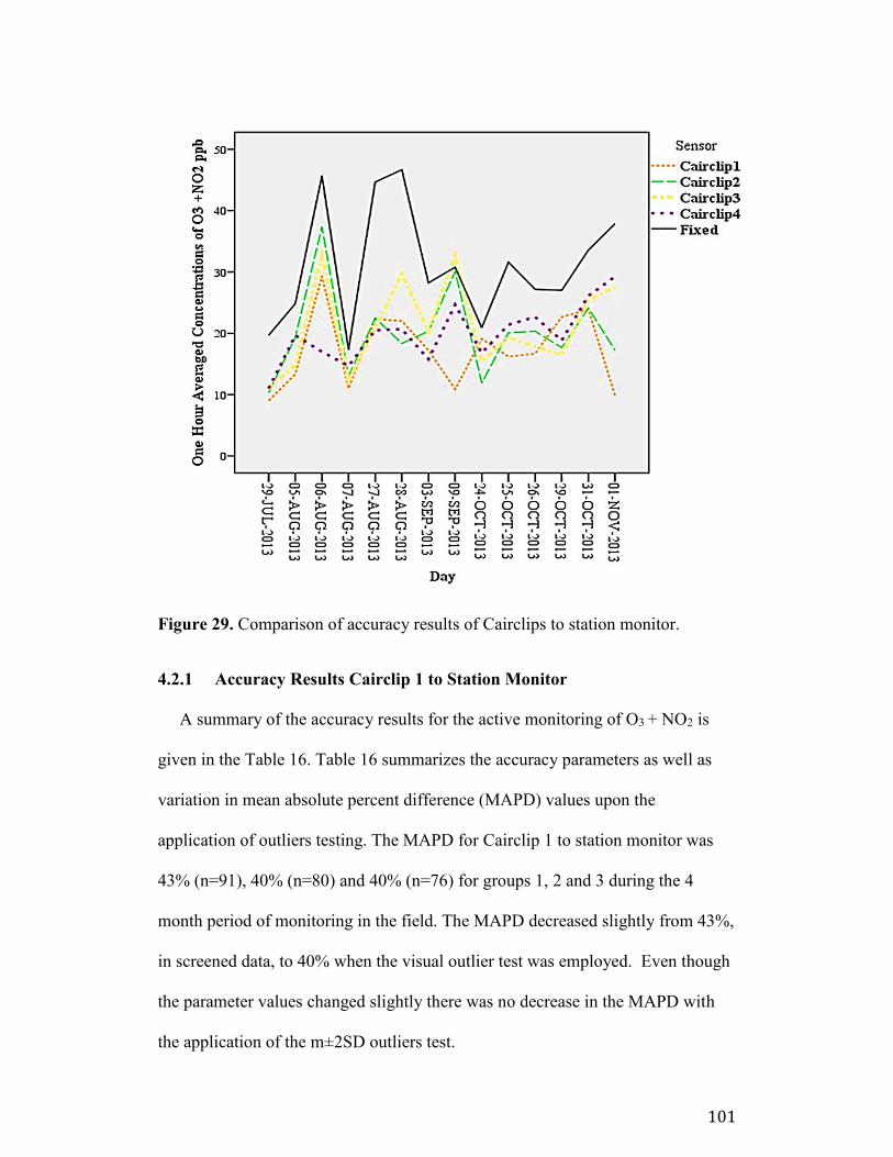
101
Figure 29. Comparison of accuracy results of Cairclips to station monitor.
4.2.1 Accuracy Results Cairclip 1 to Station Monitor
A summary of the accuracy results for the active monitoring of O3 + NO2 is
given in the Table 16. Table 16 summarizes the accuracy parameters as well as
variation in mean absolute percent difference (MAPD) values upon the
application of outliers testing. The MAPD for Cairclip 1 to station monitor was
43% (n=91), 40% (n=80) and 40% (n=76) for groups 1, 2 and 3 during the 4
month period of monitoring in the field. The MAPD decreased slightly from 43%,
in screened data, to 40% when the visual outlier test was employed. Even though
the parameter values changed slightly there was no decrease in the MAPD with
the application of the m±2SD outliers test.
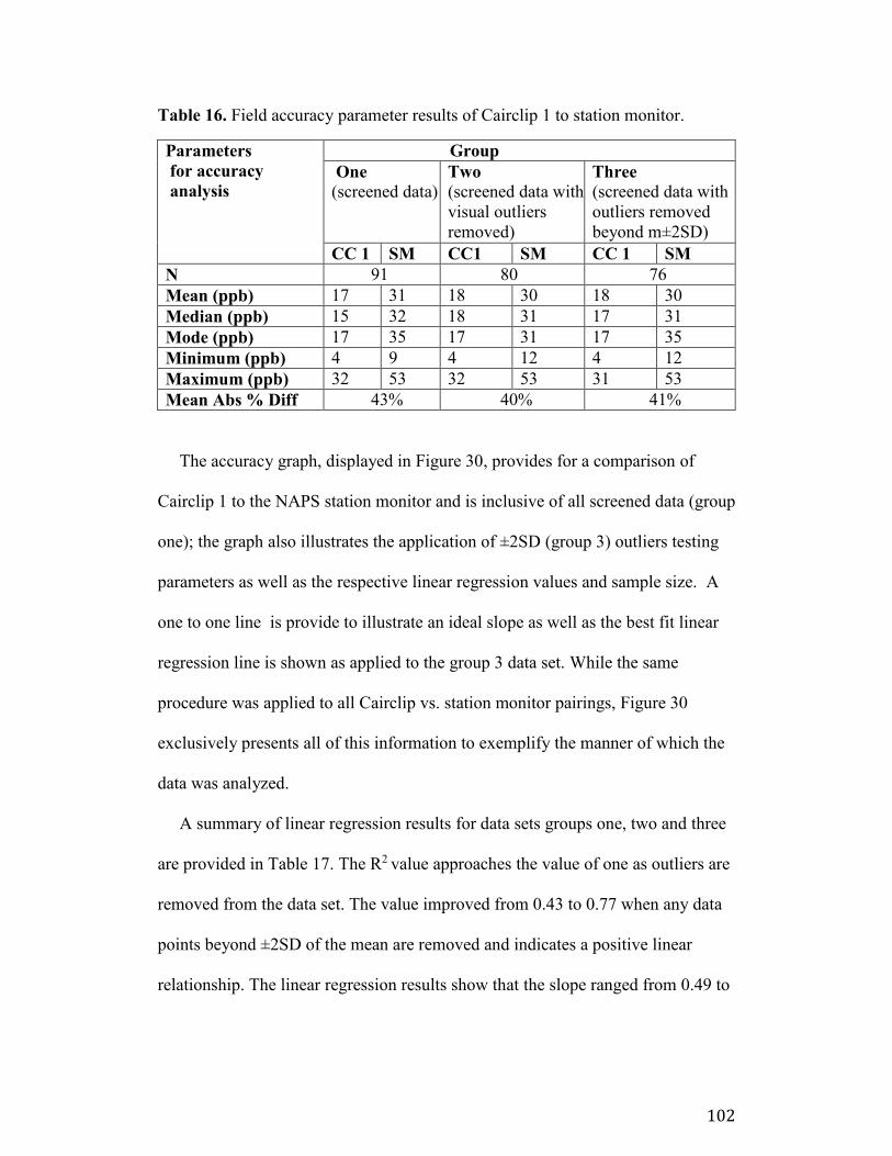
102
Table 16. Field accuracy parameter results of Cairclip 1 to station monitor.
Parameters
for accuracy
analysis
Group
One
(screened data)
Two
(screened data with
visual outliers
removed)
Three
(screened data with
outliers removed
beyond m±2SD)
CC 1 SM CC1 SM CC 1 SM
N 91 80 76
Mean (ppb) 17 31 18 30 18 30
Median (ppb) 15 32 18 31 17 31
Mode (ppb) 17 35 17 31 17 35
Minimum (ppb) 4 9 4 12 4 12
Maximum (ppb) 32 53 32 53 31 53
Mean Abs % Diff 43% 40% 41%
The accuracy graph, displayed in Figure 30, provides for a comparison of
Cairclip 1 to the NAPS station monitor and is inclusive of all screened data (group
one); the graph also illustrates the application of ±2SD (group 3) outliers testing
parameters as well as the respective linear regression values and sample size. A
one to one line is provide to illustrate an ideal slope as well as the best fit linear
regression line is shown as applied to the group 3 data set. While the same
procedure was applied to all Cairclip vs. station monitor pairings, Figure 30
exclusively presents all of this information to exemplify the manner of which the
data was analyzed.
A summary of linear regression results for data sets groups one, two and three
are provided in Table 17. The R2 value approaches the value of one as outliers are
removed from the data set. The value improved from 0.43 to 0.77 when any data
points beyond ±2SD of the mean are removed and indicates a positive linear
relationship. The linear regression results show that the slope ranged from 0.49 to
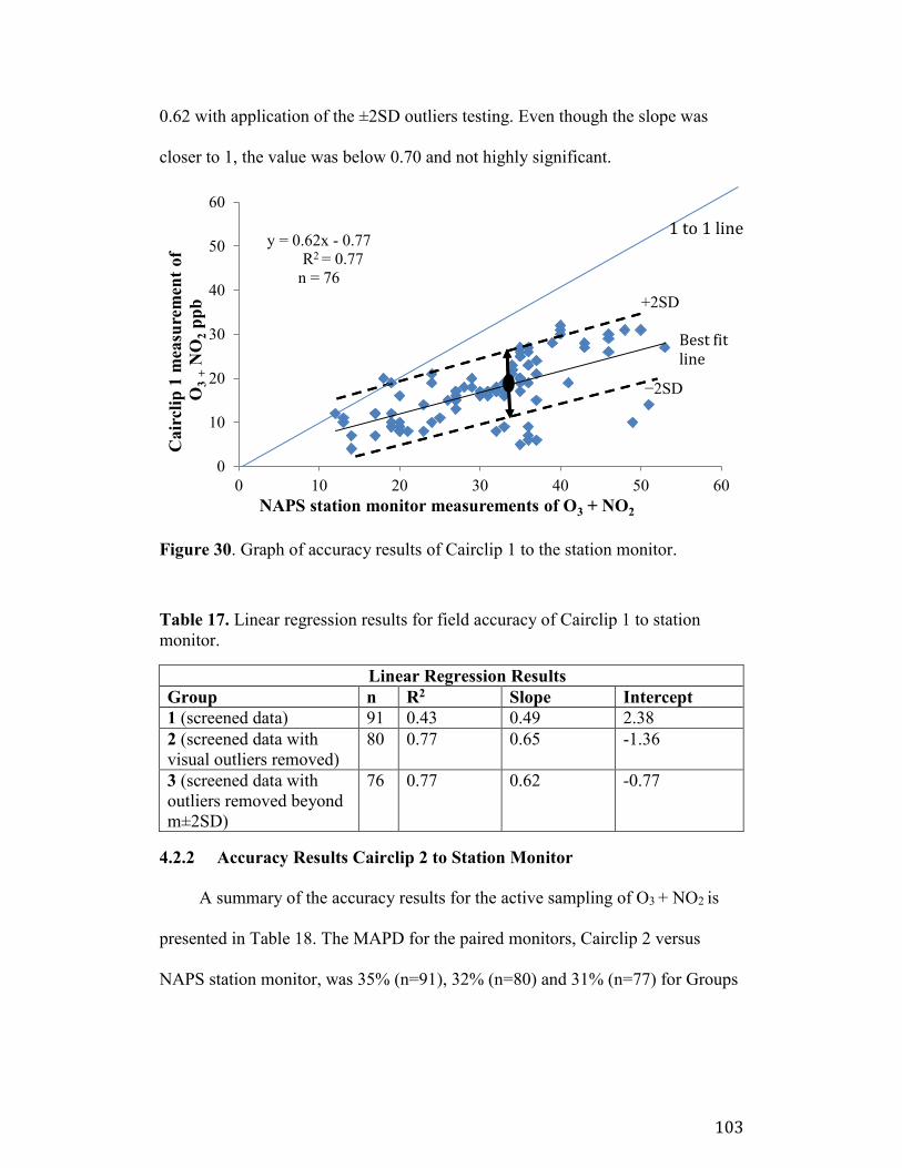
103
0.62 with application of the ±2SD outliers testing. Even though the slope was
closer to 1, the value was below 0.70 and not highly significant.
Figure 30. Graph of accuracy results of Cairclip 1 to the station monitor.
Table 17. Linear regression results for field accuracy of Cairclip 1 to station
monitor.
Linear Regression Results
Group n R2 Slope Intercept
1 (screened data) 91 0.43 0.49 2.38
2 (screened data with
visual outliers removed)
80 0.77 0.65 -1.36
3 (screened data with
outliers removed beyond
m±2SD)
76 0.77 0.62 -0.77
4.2.2 Accuracy Results Cairclip 2 to Station Monitor
A summary of the accuracy results for the active sampling of O3 + NO2 is
presented in Table 18. The MAPD for the paired monitors, Cairclip 2 versus
NAPS station monitor, was 35% (n=91), 32% (n=80) and 31% (n=77) for Groups
y = 0.62x - 0.77
R2 = 0.77
n = 76
0
10
20
30
40
50
60
0 10 20 30 40 50 60
Cair
clip
1 m
easu
rem
ent
of
O3
+N
O2
pp
b
NAPS station monitor measurements of O3 + NO2
+2SD
−2SD
Best fit line
1 to 1 line
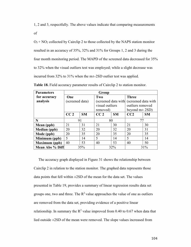
104
1, 2 and 3, respectfully. The above values indicate that comparing measurements
of
O3 + NO2 collected by Cairclip 2 to those collected by the NAPS station monitor
resulted in an accuracy of 35%, 32% and 31% for Groups 1, 2 and 3 during the
four month monitoring period. The MAPD of the screened data decreased for 35%
to 32% when the visual outliers test was employed; while a slight decrease was
incurred from 32% to 31% when the m±-2SD outlier test was applied.
Table 18. Field accuracy parameter results of Cairclip 2 to station monitor.
Parameters
for accuracy
analysis
Group
One
(screened data)
Two
(screened data with
visual outliers
removed)
Three
(screened data with
outliers removed
beyond m± 2SD)
CC 2 SM CC 2 SM CC2 SM
N 91 80 77
Mean (ppb) 21 31 21 30 21 30
Median (ppb) 20 32 20 32 20 31
Mode (ppb) 20 35 20 35 20 35
Minimum (ppb) 5 14 5 14 5 14
Maximum (ppb) 40 53 40 53 40 50
Mean Abs % Diff 35% 32% 31%
The accuracy graph displayed in Figure 31 shows the relationship between
Cairclip 2 in relation to the station monitor. The graphed data represents those
data points that fell within ±2SD of the mean for the data set. The values
presented in Table 19, provides a summary of linear regression results data set
groups one, two and three. The R2 value approaches the value of one as outliers
are removed from the data set, providing evidence of a positive linear
relationship. In summary the R2 value improved from 0.40 to 0.67 when data that
lied outside ±2SD of the mean were removed. The slope values increased from
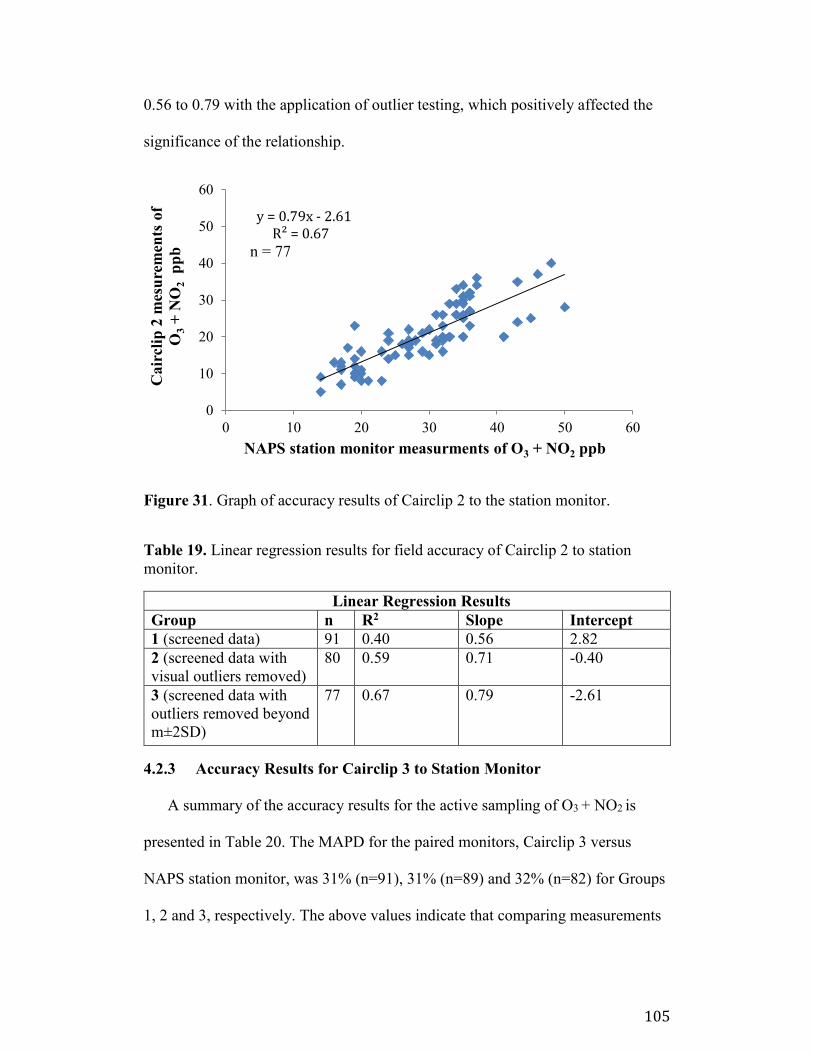
105
0.56 to 0.79 with the application of outlier testing, which positively affected the
significance of the relationship.
Figure 31. Graph of accuracy results of Cairclip 2 to the station monitor.
Table 19. Linear regression results for field accuracy of Cairclip 2 to station
monitor.
Linear Regression Results
Group n R2 Slope Intercept
1 (screened data) 91 0.40 0.56 2.82
2 (screened data with
visual outliers removed)
80 0.59 0.71 -0.40
3 (screened data with
outliers removed beyond
m±2SD)
77 0.67 0.79 -2.61
4.2.3 Accuracy Results for Cairclip 3 to Station Monitor
A summary of the accuracy results for the active sampling of O3 + NO2 is
presented in Table 20. The MAPD for the paired monitors, Cairclip 3 versus
NAPS station monitor, was 31% (n=91), 31% (n=89) and 32% (n=82) for Groups
1, 2 and 3, respectively. The above values indicate that comparing measurements
y = 0.79x - 2.61R² = 0.67
0
10
20
30
40
50
60
0 10 20 30 40 50 60
Cair
clip
2 m
esu
rem
ents
of
O3
+ N
O2
pp
b
NAPS station monitor measurments of O3 + NO2 ppb
n = 77
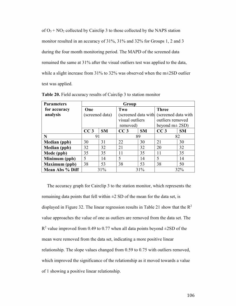
106
of O3 + NO2 collected by Cairclip 3 to those collected by the NAPS station
monitor resulted in an accuracy of 31%, 31% and 32% for Groups 1, 2 and 3
during the four month monitoring period. The MAPD of the screened data
remained the same at 31% after the visual outliers test was applied to the data,
while a slight increase from 31% to 32% was observed when the m±2SD outlier
test was applied.
Table 20. Field accuracy results of Cairclip 3 to station monitor
Parameters
for accuracy
analysis
Group
One
(screened data)
Two
(screened data with
visual outliers
removed)
Three
(screened data with
outliers removed
beyond m± 2SD)
CC 3 SM CC 3 SM CC 3 SM
N 91 89 82
Median (ppb) 30 31 22 30 21 30
Median (ppb) 32 32 21 32 20 32
Mode (ppb) 35 35 11 35 11 35
Minimum (ppb) 5 14 5 14 5 14
Maximum (ppb) 38 53 38 53 38 50
Mean Abs % Diff 31% 31% 32%
The accuracy graph for Cairclip 3 to the station monitor, which represents the
remaining data points that fell within ±2 SD of the mean for the data set, is
displayed in Figure 32. The linear regression results in Table 21 show that the R2
value approaches the value of one as outliers are removed from the data set. The
R2 value improved from 0.49 to 0.77 when all data points beyond ±2SD of the
mean were removed from the data set, indicating a more positive linear
relationship. The slope values changed from 0.59 to 0.75 with outliers removed,
which improved the significance of the relationship as it moved towards a value
of 1 showing a positive linear relationship.
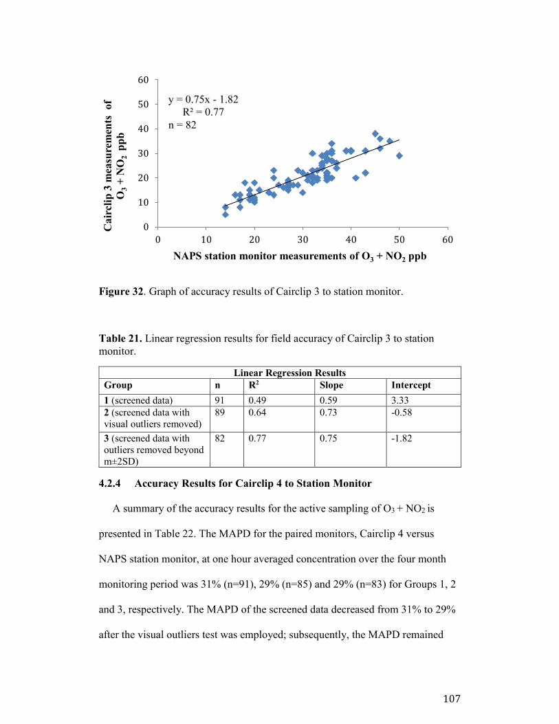
107
Figure 32. Graph of accuracy results of Cairclip 3 to station monitor.
Table 21. Linear regression results for field accuracy of Cairclip 3 to station
monitor.
Linear Regression Results
Group n R2 Slope Intercept
1 (screened data) 91 0.49 0.59 3.33
2 (screened data with
visual outliers removed)
89 0.64 0.73 -0.58
3 (screened data with
outliers removed beyond
m±2SD)
82 0.77 0.75 -1.82
4.2.4 Accuracy Results for Cairclip 4 to Station Monitor
A summary of the accuracy results for the active sampling of O3 + NO2 is
presented in Table 22. The MAPD for the paired monitors, Cairclip 4 versus
NAPS station monitor, at one hour averaged concentration over the four month
monitoring period was 31% (n=91), 29% (n=85) and 29% (n=83) for Groups 1, 2
and 3, respectively. The MAPD of the screened data decreased from 31% to 29%
after the visual outliers test was employed; subsequently, the MAPD remained
y = 0.75x - 1.82
R² = 0.77
0
10
20
30
40
50
60
0 10 20 30 40 50 60
Cair
clip
3 m
easu
rem
ents
of
O3
+ N
O2
p
pb
NAPS station monitor measurements of O3 + NO2 ppb
n = 82
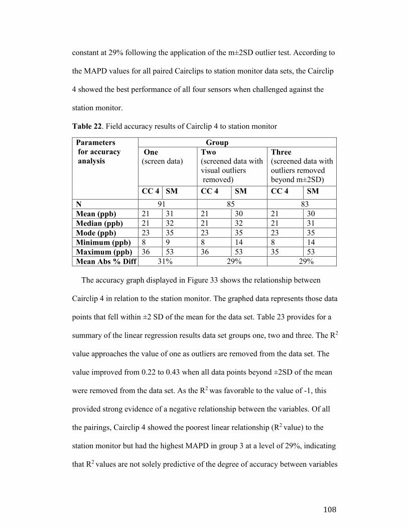
108
constant at 29% following the application of the m±2SD outlier test. According to
the MAPD values for all paired Cairclips to station monitor data sets, the Cairclip
4 showed the best performance of all four sensors when challenged against the
station monitor.
Table 22. Field accuracy results of Cairclip 4 to station monitor
Parameters
for accuracy
analysis
Group
One
(screen data)
Two
(screened data with
visual outliers
removed)
Three
(screened data with
outliers removed
beyond m±2SD)
CC 4 SM CC 4 SM CC 4 SM
N 91 85 83
Mean (ppb) 21 31 21 30 21 30
Median (ppb) 21 32 21 32 21 31
Mode (ppb) 23 35 23 35 23 35
Minimum (ppb) 8 9 8 14 8 14
Maximum (ppb) 36 53 36 53 35 53
Mean Abs % Diff 31% 29% 29%
The accuracy graph displayed in Figure 33 shows the relationship between
Cairclip 4 in relation to the station monitor. The graphed data represents those data
points that fell within ±2 SD of the mean for the data set. Table 23 provides for a
summary of the linear regression results data set groups one, two and three. The R2
value approaches the value of one as outliers are removed from the data set. The
value improved from 0.22 to 0.43 when all data points beyond ±2SD of the mean
were removed from the data set. As the R2 was favorable to the value of -1, this
provided strong evidence of a negative relationship between the variables. Of all
the pairings, Cairclip 4 showed the poorest linear relationship (R2 value) to the
station monitor but had the highest MAPD in group 3 at a level of 29%, indicating
that R2 values are not solely predictive of the degree of accuracy between variables
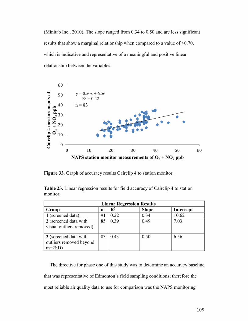
109
(Minitab Inc., 2010). The slope ranged from 0.34 to 0.50 and are less significant
results that show a marginal relationship when compared to a value of >0.70,
which is indicative and representative of a meaningful and positive linear
relationship between the variables.
Figure 33. Graph of accuracy results Cairclip 4 to station monitor.
Table 23. Linear regression results for field accuracy of Cairclip 4 to station
monitor.
Linear Regression Results
Group n R2 Slope Intercept
1 (screened data) 91 0.22 0.34 10.62
2 (screened data with
visual outliers removed)
85 0.39 0.49 7.03
3 (screened data with
outliers removed beyond
m±2SD)
83 0.43 0.50 6.56
The directive for phase one of this study was to determine an accuracy baseline
that was representative of Edmonton’s field sampling conditions; therefore the
most reliable air quality data to use for comparison was the NAPS monitoring
y = 0.50x + 6.56
R² = 0.42
0
10
20
30
40
50
60
0 10 20 30 40 50 60
Cair
clip
4 m
easu
rem
ents
of
O3
+ N
O2
pp
b
NAPS station monitor measurements of O3 + NO2 ppb
n = 83
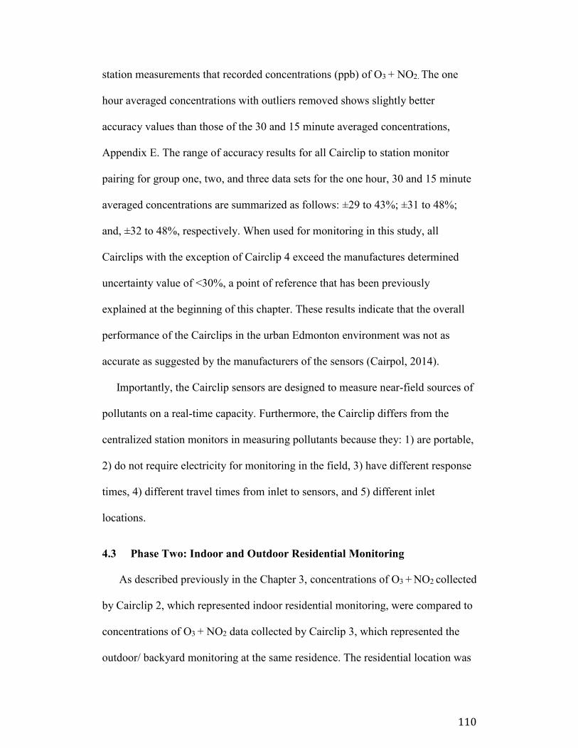
110
station measurements that recorded concentrations (ppb) of O3 + NO2. The one
hour averaged concentrations with outliers removed shows slightly better
accuracy values than those of the 30 and 15 minute averaged concentrations,
Appendix E. The range of accuracy results for all Cairclip to station monitor
pairing for group one, two, and three data sets for the one hour, 30 and 15 minute
averaged concentrations are summarized as follows: ±29 to 43%; ±31 to 48%;
and, ±32 to 48%, respectively. When used for monitoring in this study, all
Cairclips with the exception of Cairclip 4 exceed the manufactures determined
uncertainty value of <30%, a point of reference that has been previously
explained at the beginning of this chapter. These results indicate that the overall
performance of the Cairclips in the urban Edmonton environment was not as
accurate as suggested by the manufacturers of the sensors (Cairpol, 2014).
Importantly, the Cairclip sensors are designed to measure near-field sources of
pollutants on a real-time capacity. Furthermore, the Cairclip differs from the
centralized station monitors in measuring pollutants because they: 1) are portable,
2) do not require electricity for monitoring in the field, 3) have different response
times, 4) different travel times from inlet to sensors, and 5) different inlet
locations.
4.3 Phase Two: Indoor and Outdoor Residential Monitoring
As described previously in the Chapter 3, concentrations of O3 + NO2 collected
by Cairclip 2, which represented indoor residential monitoring, were compared to
concentrations of O3 + NO2 data collected by Cairclip 3, which represented the
outdoor/ backyard monitoring at the same residence. The residential location was
111
in a core neighborhood in Edmonton located at 88th Avenue and 98th Street and is
shown on the map provided in Figure 34.
Figure 34. Map showing approximate location of residential monitoring.
Monthly and hourly intervals were established in order to compare
concentrations for 6 to 9 am, 10 am to 1 pm, 2 to 5 pm and finally 6 to 7 pm,
Table 25. The graph provided in Figure 37, compares the ratios of the data from
Cairclip 2 to Cairclip 3 in relation to hourly ranges as indicated in Table 24.
An arbitrary value of 1 was set to distinguish outdoor from indoor, with ratios
less than 1 (<1) meaning outdoor concentrations measured in ppb of O3 + NO2
were higher than that of the indoor concentrations. In general, it was observed that
the residential outdoor near-field concentrations were higher than indoor near-
Residential
Monitoring
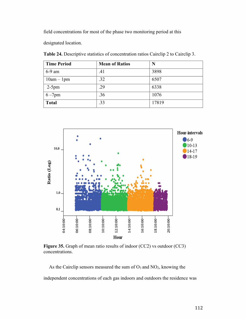
112
field concentrations for most of the phase two monitoring period at this
designated location.
Table 24. Descriptive statistics of concentration ratios Cairclip 2 to Cairclip 3.
Time Period Mean of Ratios N
6-9 am .41 3898
10am – 1pm .32 6507
2-5pm .29 6338
6 –7pm .36 1076
Total .33 17819
Figure 35. Graph of mean ratio results of indoor (CC2) vs outdoor (CC3)
concentrations.
As the Cairclip sensors measured the sum of O3 and NO2, knowing the
independent concentrations of each gas indoors and outdoors the residence was
113
not possible. This said, inferences can be made based on aspects and qualities of
the indoor and outdoor environment in question. Characteristics of the house such
as the style, age, location, types of heating systems and level of human activity
can provide valuable information in understanding why indoor concentrations of
O3 + NO2 were lower than outdoor residential concentrations.
The home used for monitoring in this study was a 1940’s bungalow that was
not highly insulated or sealed; therefore this may have influenced the
concentration levels of O3 + NO2 present indoors. These structural elements
inherent in the home may have encouraged air flow and mixing of ambient
outdoor air into the indoor environment. The main reason for low concentrations
of O3 and NO2 was due to the scavenging process and because there was low
production of these gases in the home.
The outdoor air that infiltrates to the indoor environment may affect indoor air
quality particularly when attempting to measure highly reactive gases, such as O3
and NO2. This is explained as NO2 can undergo photolysis, which transforms it
into NO and O2. The O2 atoms rapidly react with molecular oxygen to form O3.
Simultaneously, NO quickly scavenges for O3 resulting in the formation of NO2
and O2 (US EPA, 2014e). O3 is a powerful oxidizing agent, its capacity to react
quickly with other chemicals in the air acts to create other by-products. Because
of the high capacity of this air mixing phenomenon with other residual parameters
within the indoor environment, concentrations of O3 + NO2 once present are
quickly changed. Because of the highly reactive and scavenging character of these
114
gases, the Cairclip may not have been capable of measuring concentrations as
they were already transformed into other chemical compounds (WHO, 2003b).
4.4 Phase Two: Personal Exposure Monitoring
In the personal exposure portion of the study, Cairclip sensors 1 and 4 were used to
measure exposure to O3 + NO2 as an individual carried out their various daily
activities. The objective of this part of the study was to select scenario locations
that captured near-field exposure to the pollutants, O3 and NO2, representative of
the average person’s daily routine in an urban environment.
The Cairclips are designed to measure exposure to concentrations of O3 + NO2
in relation to time-activity patterns that represent the unique behaviors’ of an
individual in the microenvironments with which they interact. Whereas, the fixed-
site centralized monitors such as the Edmonton south station monitor (ESSM) and
the Edmonton central station monitor( ECSM), provide concentration
measurements of criteria pollutants based on their localized ambient area
(Nejadkooki et al., 2011; Ott, 2007a). Both monitoring technologies are designed
to measure ambient concentrations of O3 + NO2, the source of pollution differs.
The centralized stations measure far-field sources while the Cairclip is designed
to measure near-field sources at the receptor, in this case a person (Ott, 2007a;
Cairpol, 2014).
Through monitoring with the Cairclips, the personal exposure portion of the
study aimed to show the degree of variation between concentrations of pollutants
measured at the individual level based on varied spatio-temporal conditions with
that of concentrations measured by centralized monitoring. Consideration of the
115
degree and duration of exposure to concentration to O3 + NO2 were instrumental
to assessing the potential human exposure to these pollutants as related to certain
urban locations.
For purposes of this study, the reference value for comparison used with be a
sum concentration of 240 ppb which was calculated by adding the one-hour
Alberta Ambient Air Quality Objectives for O3 at 80 ppb and NO2 at 160 ppb,
respectively. The data presented in this part of phase two includes only the
monitoring times that showed significant eventful concentrations, i.e.
concentration spikes above those of the station monitor. In addition to this, only
those monitoring events that exceed the Cairclip’s limit of detection (LOD) of 20
ppb were considered relevant for discussion (Cairpol, 2014).
The ECSM located on the top of a building downtown Edmonton located on
104th Avenue between 109th and 110th Streets and is meant to be representative of
urban core exposures to concentrations of O3 + NO2 whereas, the ESSM in the
southwest side of the city is meant to be representative of residential ambient air
concentrations of O3 + NO2. The discussion includes findings from various
settings that were monitored with Cairclips 1 and 4 which are contrasted with the
centralized station monitor as a means of reference.
4.5 Monitoring of Busy Intersections and Roadways
In this environmental setting, the personal exposure scenarios pertained to
monitoring outdoor sites on foot at high volume traffic areas located in urban core
areas. The intersections of interest were chosen to represent a comparison of two
downtown locations, as well as two locations in the Whyte Avenue vicinity.
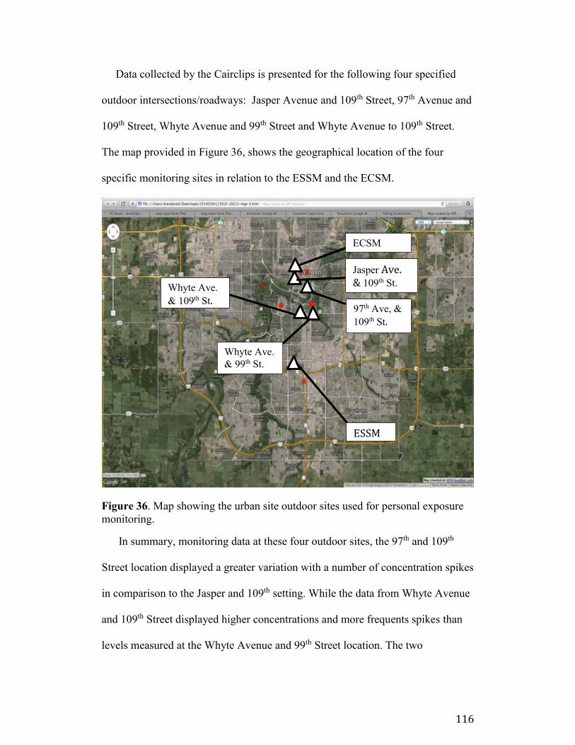
116
Data collected by the Cairclips is presented for the following four specified
outdoor intersections/roadways: Jasper Avenue and 109th Street, 97th Avenue and
109th Street, Whyte Avenue and 99th Street and Whyte Avenue to 109th Street.
The map provided in Figure 36, shows the geographical location of the four
specific monitoring sites in relation to the ESSM and the ECSM.
Figure 36. Map showing the urban site outdoor sites used for personal exposure
monitoring.
In summary, monitoring data at these four outdoor sites, the 97th and 109th
Street location displayed a greater variation with a number of concentration spikes
in comparison to the Jasper and 109th setting. While the data from Whyte Avenue
and 109th Street displayed higher concentrations and more frequents spikes than
levels measured at the Whyte Avenue and 99th Street location. The two
Whyte Ave.
& 99th St.
Whyte Ave.
& 109th St.
ECSM
Jasper Ave. & 109th St.
97th Ave, &
109th St.
ESSM
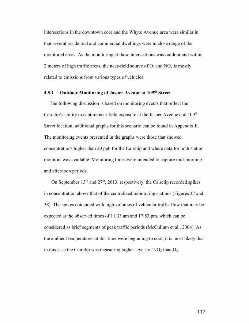
117
intersections in the downtown core and the Whyte Avenue area were similar in
that several residential and commercial dwellings were in close range of the
monitored areas. As the monitoring at these intersections was outdoor and within
2 meters of high traffic areas, the near-field source of O3 and NO2 is mostly
related to emissions from various types of vehicles.
4.5.1 Outdoor Monitoring of Jasper Avenue at 109th Street
The following discussion is based on monitoring events that reflect the
Cairclip’s ability to capture near field exposure at the Jasper Avenue and 109th
Street location, additional graphs for this scenario can be found in Appendix E.
The monitoring events presented in the graphs were those that showed
concentrations higher than 20 ppb for the Cairclip and where data for both station
monitors was available. Monitoring times were intended to capture mid-morning
and afternoon periods.
On September 13th and 27th, 2013, respectively, the Cairclip recorded spikes
in concentration above that of the centralized monitoring stations (Figures 37 and
38). The spikes coincided with high volumes of vehicular traffic flow that may be
expected at the observed times of 11:33 am and 17:53 pm, which can be
considered as brief segments of peak traffic periods (McCullum et al., 2004). As
the ambient temperatures at this time were beginning to cool, it is most likely that
in this case the Cairclip was measuring higher levels of NO2 than O3.
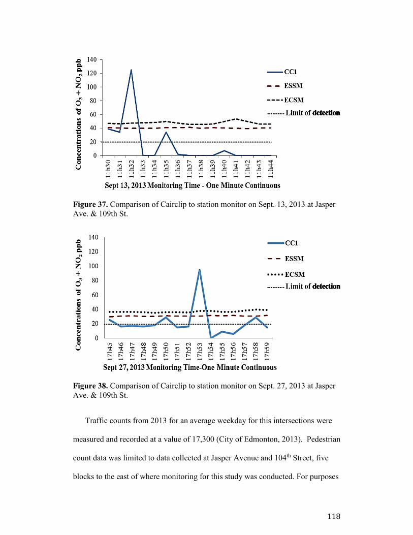
118
Figure 37. Comparison of Cairclip to station monitor on Sept. 13, 2013 at Jasper
Ave. & 109th St.
Figure 38. Comparison of Cairclip to station monitor on Sept. 27, 2013 at Jasper
Ave. & 109th St.
Traffic counts from 2013 for an average weekday for this intersections were
measured and recorded at a value of 17,300 (City of Edmonton, 2013). Pedestrian
count data was limited to data collected at Jasper Avenue and 104th Street, five
blocks to the east of where monitoring for this study was conducted. For purposes
119
of this study, the pedestrian counts at a mid-day peak of 292 was assumed as a
reference value to representative of pedestrian activity in this area (Gresiuk,
2013). It was observed and recorded in the time activity diary that, for this
location, pedestrian volumes varied from light to moderate dependent upon the
time of day.
The findings at the Jasper Avenue and 109th Street location showed that while
both the centralized monitoring stations measured concentrations of O3 + NO2 at a
relatively stable and consistent level, the Cairclips showed greater variability.
Although the Cairclips recorded spikes in concentrations of O3 + NO2, there were
no events that exceeded the reference value of 240 ppb. Furthermore, the
concentration spikes that were observed were limited to one to three minutes in
durations.
4.5.2 Outdoor Monitoring at 97th Avenue and 109th Street
Findings at the 97th Avenue and 109th Street location are discussed in the
following. Weekday traffic counts at this intersection have been measured at
33,300 (City of Edmonton, 2013). Although pedestrian counts have not yet been
measured, it was observed that a high number of commuters travelled this area by
bicycle and foot to and from the downtown core. This location is centered in the
hub of the city, close to government buildings and residential developments.
Throughout the duration of monitoring at this location there was a one-time event
recorded on October 10, 2013 at 10:00 am where Cairclip 1 recorded a short term
concentration of 255 ppb, a level that exceeded the reference value of 240 ppb
(Figure 39).
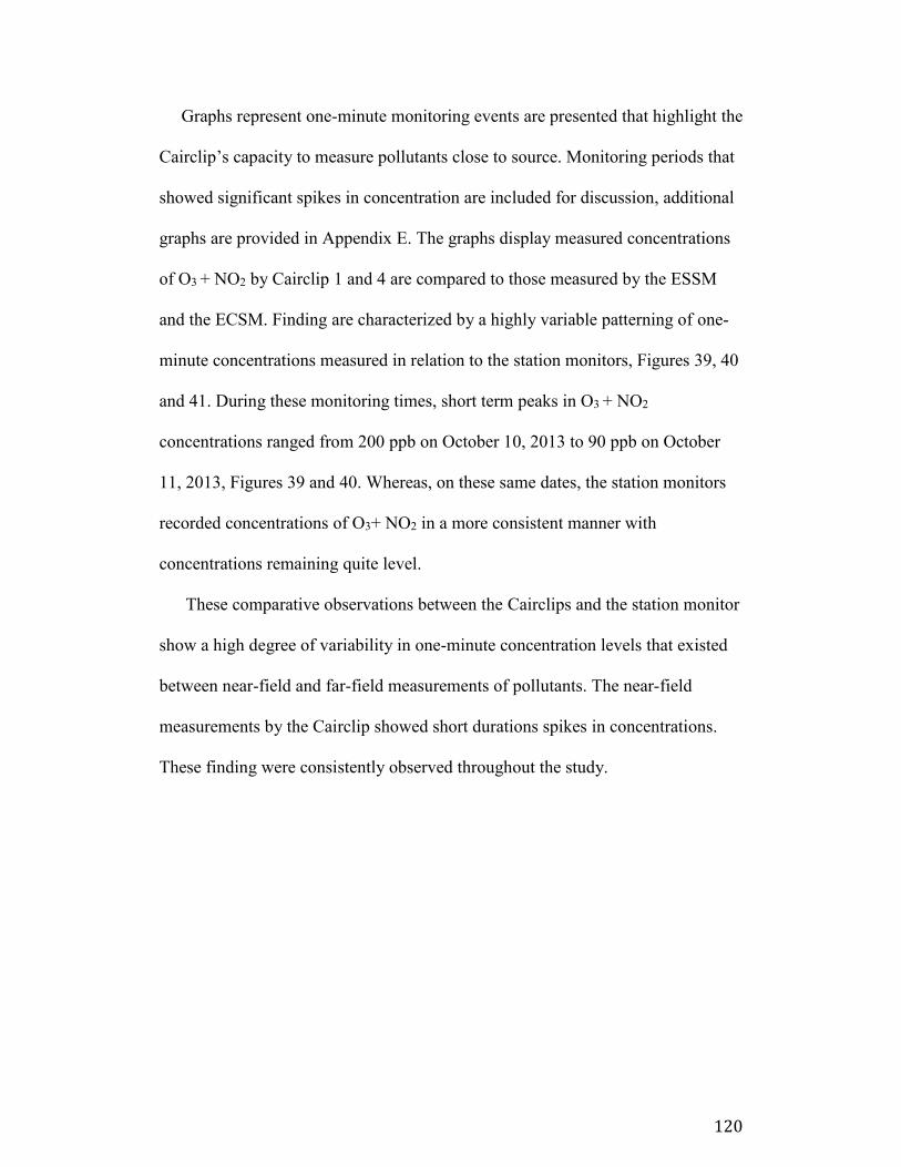
120
Graphs represent one-minute monitoring events are presented that highlight the
Cairclip’s capacity to measure pollutants close to source. Monitoring periods that
showed significant spikes in concentration are included for discussion, additional
graphs are provided in Appendix E. The graphs display measured concentrations
of O3 + NO2 by Cairclip 1 and 4 are compared to those measured by the ESSM
and the ECSM. Finding are characterized by a highly variable patterning of one-
minute concentrations measured in relation to the station monitors, Figures 39, 40
and 41. During these monitoring times, short term peaks in O3 + NO2
concentrations ranged from 200 ppb on October 10, 2013 to 90 ppb on October
11, 2013, Figures 39 and 40. Whereas, on these same dates, the station monitors
recorded concentrations of O3+ NO2 in a more consistent manner with
concentrations remaining quite level.
These comparative observations between the Cairclips and the station monitor
show a high degree of variability in one-minute concentration levels that existed
between near-field and far-field measurements of pollutants. The near-field
measurements by the Cairclip showed short durations spikes in concentrations.
These finding were consistently observed throughout the study.
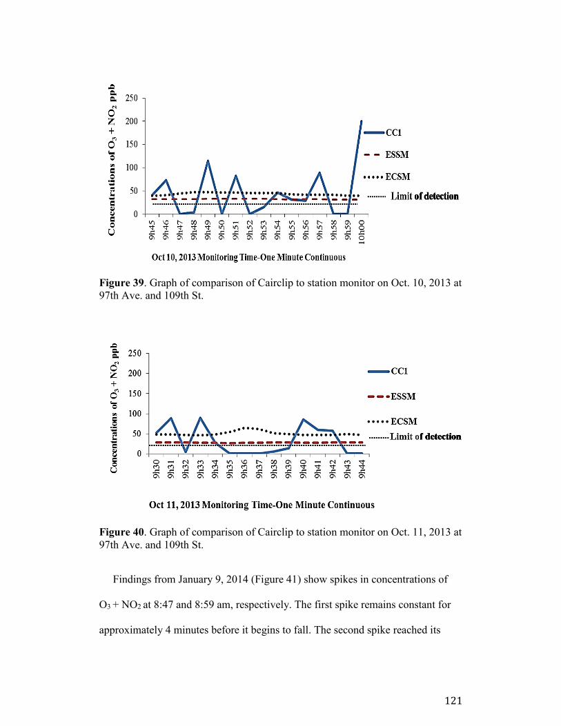
121
Figure 39. Graph of comparison of Cairclip to station monitor on Oct. 10, 2013 at
97th Ave. and 109th St.
Figure 40. Graph of comparison of Cairclip to station monitor on Oct. 11, 2013 at
97th Ave. and 109th St.
Findings from January 9, 2014 (Figure 41) show spikes in concentrations of
O3 + NO2 at 8:47 and 8:59 am, respectively. The first spike remains constant for
approximately 4 minutes before it begins to fall. The second spike reached its
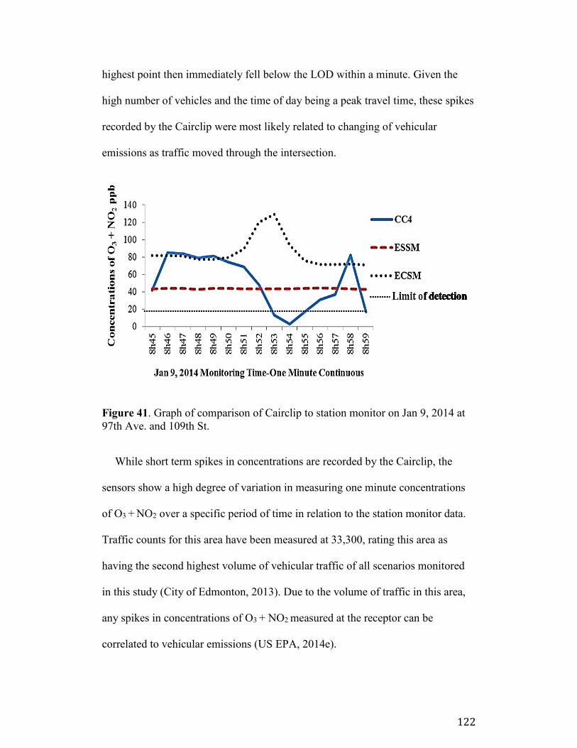
122
highest point then immediately fell below the LOD within a minute. Given the
high number of vehicles and the time of day being a peak travel time, these spikes
recorded by the Cairclip were most likely related to changing of vehicular
emissions as traffic moved through the intersection.
Figure 41. Graph of comparison of Cairclip to station monitor on Jan 9, 2014 at
97th Ave. and 109th St.
While short term spikes in concentrations are recorded by the Cairclip, the
sensors show a high degree of variation in measuring one minute concentrations
of O3 + NO2 over a specific period of time in relation to the station monitor data.
Traffic counts for this area have been measured at 33,300, rating this area as
having the second highest volume of vehicular traffic of all scenarios monitored
in this study (City of Edmonton, 2013). Due to the volume of traffic in this area,
any spikes in concentrations of O3 + NO2 measured at the receptor can be
correlated to vehicular emissions (US EPA, 2014e).
123
4.5.3 Outdoor Monitoring of Whyte Avenue to 109th Street
Traffic count data collected for Whyte Avenue in 2012 measured weekday
volumes in the range of 22,000 to 24,600 and pedestrian counts ranged from
approximately 320 to 2400 (Gresiuk, 2012; City of Edmonton, 2013). A time
interval of thirty minutes was selected for this particular scenario.
As in previous discussions of other monitoring scenarios, the Cairclip sensors
generally measured concentrations of O3 + NO2 lower than that of the station
monitors. Figures 42 and 43 are provided as specific examples of the monitoring
results of the Cairclips at this monitoring site, additional graphs are available in
Appendix E. As displayed in Figure 42, the overall performance of Cairclip shows
that exposures at the personal, real time level were much lower than
concentrations recorded by the ECSM. However, on this date Cairclip 4 records a
one minute spike at the end of the monitoring period at 1:59 pm with a level of 75
ppb. The concentrations measured by Cairclip 4 were climbing while the ECSM
were steady. The ESSM data remaining consistent at a much lower concentration.
On December 23, 2013 the Cairclip shows a highly variable pattern based on
one minute averaged concentrations which ranged from approximately 80 to 120
ppb throughout the 30 minute monitoring period (Figure 43). The time of day
ranges from 17:30 to 17:59 pm which correlates with rush hour times of traffic,
and subsequent higher concentrations of vehicular emissions.
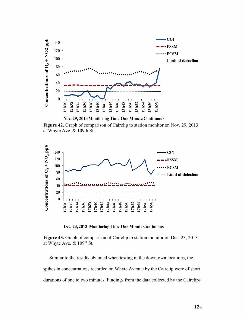
124
Figure 42. Graph of comparison of Cairclip to station monitor on Nov. 29, 2013
at Whyte Ave. & 109th St.
Figure 43. Graph of comparison of Cairclip to station monitor on Dec. 23, 2013
at Whyte Ave. & 109th St.
Similar to the results obtained when testing in the downtown locations, the
spikes in concentrations recorded on Whyte Avenue by the Cairclip were of short
durations of one to two minutes. Findings from the data collected by the Cairclips
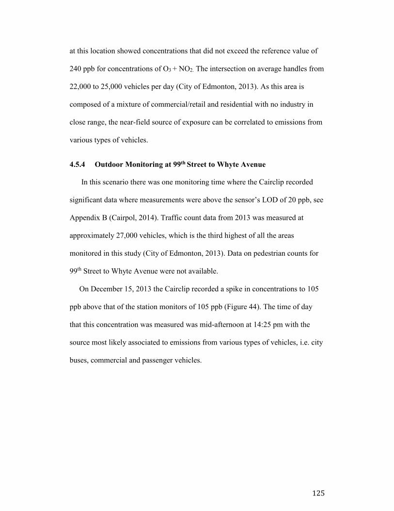
125
at this location showed concentrations that did not exceed the reference value of
240 ppb for concentrations of O3 + NO2. The intersection on average handles from
22,000 to 25,000 vehicles per day (City of Edmonton, 2013). As this area is
composed of a mixture of commercial/retail and residential with no industry in
close range, the near-field source of exposure can be correlated to emissions from
various types of vehicles.
4.5.4 Outdoor Monitoring at 99th Street to Whyte Avenue
In this scenario there was one monitoring time where the Cairclip recorded
significant data where measurements were above the sensor’s LOD of 20 ppb, see
Appendix B (Cairpol, 2014). Traffic count data from 2013 was measured at
approximately 27,000 vehicles, which is the third highest of all the areas
monitored in this study (City of Edmonton, 2013). Data on pedestrian counts for
99th Street to Whyte Avenue were not available.
On December 15, 2013 the Cairclip recorded a spike in concentrations to 105
ppb above that of the station monitors of 105 ppb (Figure 44). The time of day
that this concentration was measured was mid-afternoon at 14:25 pm with the
source most likely associated to emissions from various types of vehicles, i.e. city
buses, commercial and passenger vehicles.

126
Figure 44. Graph of comparison of Cairclip to station monitor on Dec. 15, 2013
at 99th St. & Whyte Ave.
Similar to the other areas monitored in this scenario of phase two, the near-
field source of exposure measured by the Cairclip can be attributed to vehicular
emissions. In consideration of the reference value of 240 ppb, the Cairclip data
showed only short term spikes of concentrations of O3 + NO2 that were far below
this value.
As a general observation, monitoring data from the intersections and roadways
show that the ambient monitors, ESSM and ECSM, measured concentrations of
O3 + NO2 in a consistent and level pattern. Conversely, the Cairclips periodically
showed a high degree of variation in concentration measurements of O3 + NO2
from minute to minute throughout the course of the monitoring times. These
variations in concentrations from minute to minute are characteristic of the active,

127
personal Cairclip samplers, as they measure near-field sources of pollutants in a
real time capacity.
4.6 Commuter Monitoring on Public Transit: LRT and Bus
In this study, for purposes of measuring personal exposure to O3 + NO2,
monitoring using the Cairclip was conducted on both a city transit bus and on
light rail transport (LRT). The rational for choosing to monitor on public transit
was to determine the concentration level of potential exposures to O3 + NO2
correlated to time of day and location while commuting. The following are the
important findings of monitoring on public transit: peak concentrations ranging
from 60 ppb to 150 ppb were measured on the bus at various locations on route to
the West Edmonton Mall (WEM) transit station and during wait times at station,
both inside and outside the bus; concentration spikes measured on LRT were
more commonly observed during north-bound travel from SG to Grandin and in
LRT stations following train departure.
4.6.1 Monitoring on Bus Route #33: Southgate to West Edmonton Mall
The commuting scenario chosen for travelling via a city bus was route #33
from the Southgate station to the West Edmonton Mall transit station and return
(Figure 19). When possible, the air monitoring was conducted from the middle
section of the bus for consistency.
Some monitoring events were removed from this analysis because of missing
data from the ambient station monitors due to maintenance or malfunctions which
interrupted data collection. Consistent with the findings from other monitoring
scenarios, the Cairclip demonstrated a high rate of variation during this
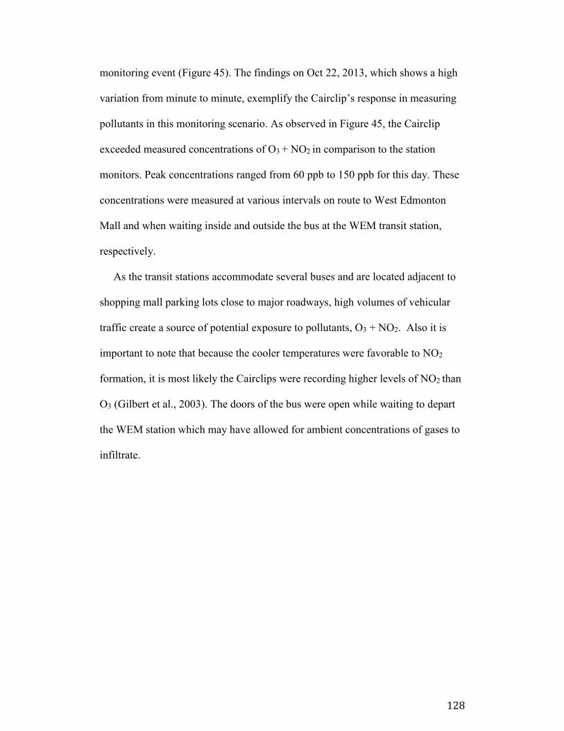
128
monitoring event (Figure 45). The findings on Oct 22, 2013, which shows a high
variation from minute to minute, exemplify the Cairclip’s response in measuring
pollutants in this monitoring scenario. As observed in Figure 45, the Cairclip
exceeded measured concentrations of O3 + NO2 in comparison to the station
monitors. Peak concentrations ranged from 60 ppb to 150 ppb for this day. These
concentrations were measured at various intervals on route to West Edmonton
Mall and when waiting inside and outside the bus at the WEM transit station,
respectively.
As the transit stations accommodate several buses and are located adjacent to
shopping mall parking lots close to major roadways, high volumes of vehicular
traffic create a source of potential exposure to pollutants, O3 + NO2. Also it is
important to note that because the cooler temperatures were favorable to NO2
formation, it is most likely the Cairclips were recording higher levels of NO2 than
O3 (Gilbert et al., 2003). The doors of the bus were open while waiting to depart
the WEM station which may have allowed for ambient concentrations of gases to
infiltrate.
129
Figure 45. Graph of comparison of Cairclip to station monitor on bus route #33
on Oct. 22, 2013
Note: Spikes are as follows: A: Heading west on 50th Ave. at 113th Street;
B: Meadowlark Road and 87th Avenue; C: WEM station; D: WEM station;
E: On return trip to SG station; G: Adjacent to Mitchener Park at 50th Avenue
and 122 Street; and H: 50th Avenue and 111th Street.
4.6.2 Monitoring on LRT Routes from Century Park to Grandin Station
In this study, air monitoring of LRT routes was conducted as a means to
quantify potential exposure to O3 + NO2 during commuting. The results of data
collection by Cairclips 1 and 4 on LRT routes are presented in the following
presentations and discussion (Figures 46 to 50). The routes monitored can be
found in Figure 19.
Monitoring times for this exposure scenario vary due to factors, which could
not be controlled for such as slight time variations of train schedule. Much of the
data presented in graphs is based on return trips. Monitoring periods on the LRT
showed breaks in the time variable in order to account for data collection in other
locations of interest as extensions from the LRT. For example, northbound LRT
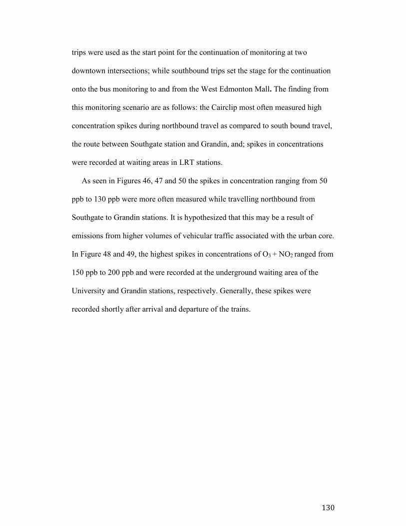
130
trips were used as the start point for the continuation of monitoring at two
downtown intersections; while southbound trips set the stage for the continuation
onto the bus monitoring to and from the West Edmonton Mall. The finding from
this monitoring scenario are as follows: the Cairclip most often measured high
concentration spikes during northbound travel as compared to south bound travel,
the route between Southgate station and Grandin, and; spikes in concentrations
were recorded at waiting areas in LRT stations.
As seen in Figures 46, 47 and 50 the spikes in concentration ranging from 50
ppb to 130 ppb were more often measured while travelling northbound from
Southgate to Grandin stations. It is hypothesized that this may be a result of
emissions from higher volumes of vehicular traffic associated with the urban core.
In Figure 48 and 49, the highest spikes in concentrations of O3 + NO2 ranged from
150 ppb to 200 ppb and were recorded at the underground waiting area of the
University and Grandin stations, respectively. Generally, these spikes were
recorded shortly after arrival and departure of the trains.
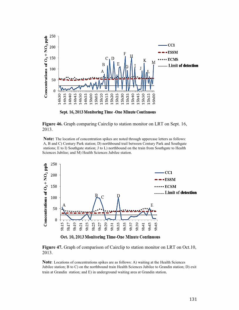
131
Figure 46. Graph comparing Cairclip to station monitor on LRT on Sept. 16,
2013.
Note: The location of concentration spikes are noted through uppercase letters as follows:
A, B and C) Century Park station; D) northbound trail between Century Park and Southgate
stations; E to I) Southgate station; J to L) northbound on the train from Southgate to Health
Sciences Jubilee; and M) Health Sciences Jubilee station.
Figure 47. Graph of comparison of Cairclip to station monitor on LRT on Oct.10,
2013.
Note: Locations of concentrations spikes are as follows: A) waiting at the Health Sciences
Jubilee station; B to C) on the northbound train Health Sciences Jubilee to Grandin station; D) exit
train at Grandin station; and E) in underground waiting area at Grandin station.
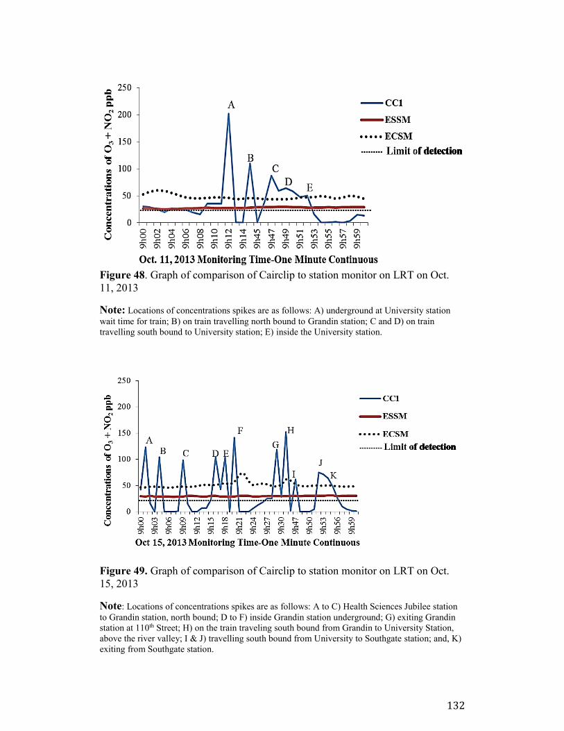
132
Figure 48. Graph of comparison of Cairclip to station monitor on LRT on Oct.
11, 2013
Note: Locations of concentrations spikes are as follows: A) underground at University station
wait time for train; B) on train travelling north bound to Grandin station; C and D) on train
travelling south bound to University station; E) inside the University station.
Figure 49. Graph of comparison of Cairclip to station monitor on LRT on Oct.
15, 2013
Note: Locations of concentrations spikes are as follows: A to C) Health Sciences Jubilee station
to Grandin station, north bound; D to F) inside Grandin station underground; G) exiting Grandin
station at 110th Street; H) on the train traveling south bound from Grandin to University Station,
above the river valley; I & J) travelling south bound from University to Southgate station; and, K)
exiting from Southgate station.
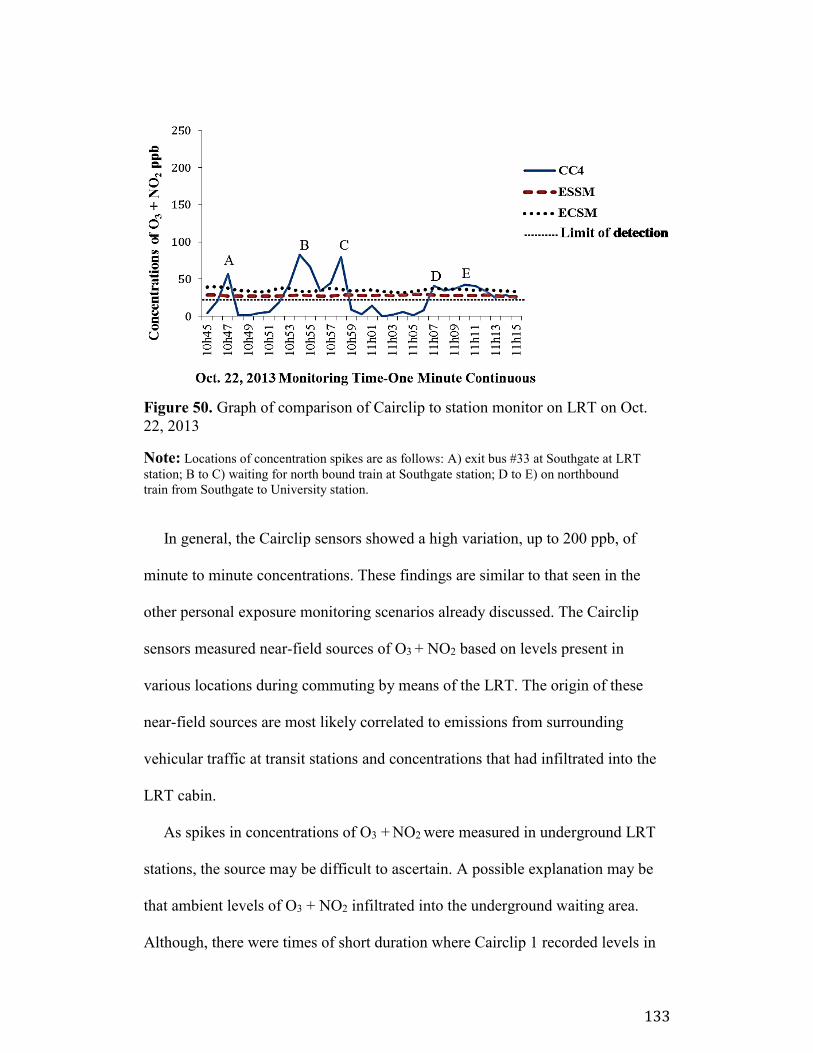
133
Figure 50. Graph of comparison of Cairclip to station monitor on LRT on Oct.
22, 2013
Note: Locations of concentration spikes are as follows: A) exit bus #33 at Southgate at LRT
station; B to C) waiting for north bound train at Southgate station; D to E) on northbound
train from Southgate to University station.
In general, the Cairclip sensors showed a high variation, up to 200 ppb, of
minute to minute concentrations. These findings are similar to that seen in the
other personal exposure monitoring scenarios already discussed. The Cairclip
sensors measured near-field sources of O3 + NO2 based on levels present in
various locations during commuting by means of the LRT. The origin of these
near-field sources are most likely correlated to emissions from surrounding
vehicular traffic at transit stations and concentrations that had infiltrated into the
LRT cabin.
As spikes in concentrations of O3 + NO2 were measured in underground LRT
stations, the source may be difficult to ascertain. A possible explanation may be
that ambient levels of O3 + NO2 infiltrated into the underground waiting area.
Although, there were times of short duration where Cairclip 1 recorded levels in
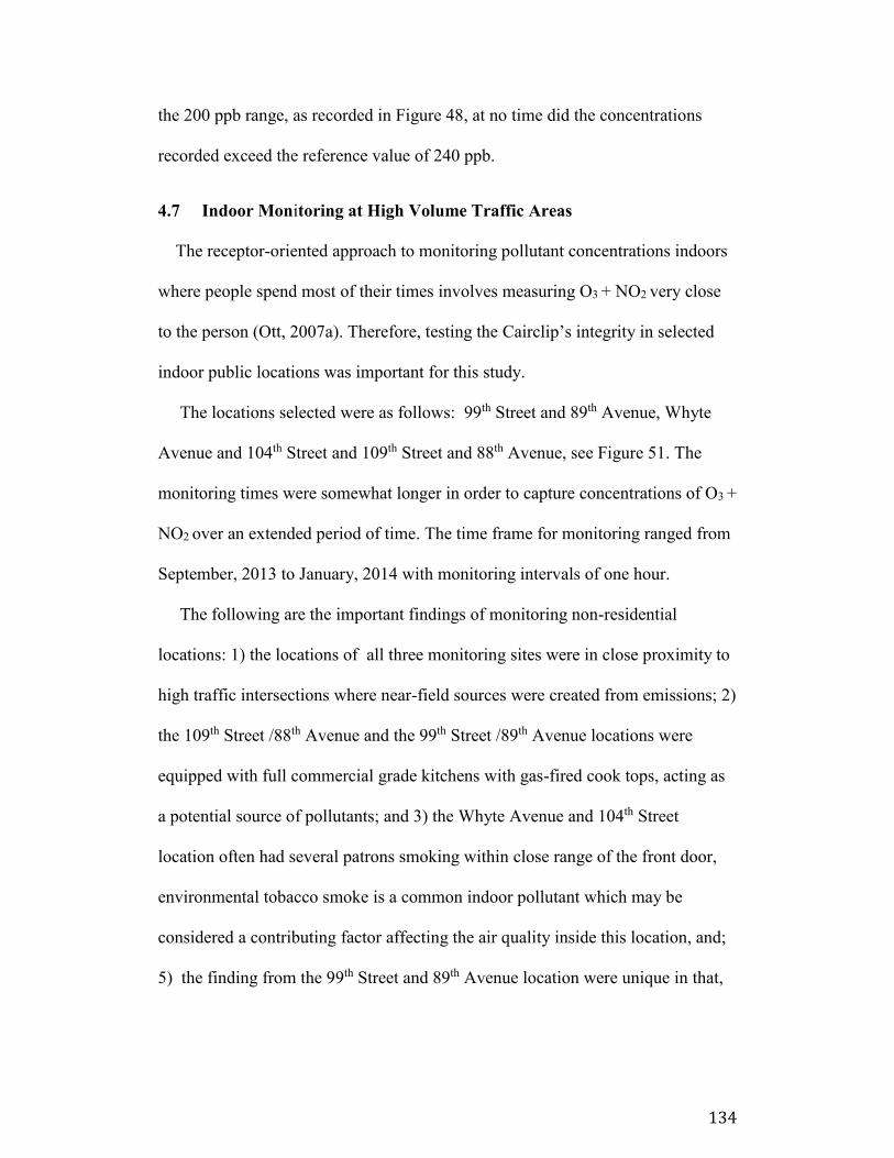
134
the 200 ppb range, as recorded in Figure 48, at no time did the concentrations
recorded exceed the reference value of 240 ppb.
4.7 Indoor Monitoring at High Volume Traffic Areas
The receptor-oriented approach to monitoring pollutant concentrations indoors
where people spend most of their times involves measuring O3 + NO2 very close
to the person (Ott, 2007a). Therefore, testing the Cairclip’s integrity in selected
indoor public locations was important for this study.
The locations selected were as follows: 99th Street and 89th Avenue, Whyte
Avenue and 104th Street and 109th Street and 88th Avenue, see Figure 51. The
monitoring times were somewhat longer in order to capture concentrations of O3 +
NO2 over an extended period of time. The time frame for monitoring ranged from
September, 2013 to January, 2014 with monitoring intervals of one hour.
The following are the important findings of monitoring non-residential
locations: 1) the locations of all three monitoring sites were in close proximity to
high traffic intersections where near-field sources were created from emissions; 2)
the 109th Street /88th Avenue and the 99th Street /89th Avenue locations were
equipped with full commercial grade kitchens with gas-fired cook tops, acting as
a potential source of pollutants; and 3) the Whyte Avenue and 104th Street
location often had several patrons smoking within close range of the front door,
environmental tobacco smoke is a common indoor pollutant which may be
considered a contributing factor affecting the air quality inside this location, and;
5) the finding from the 99th Street and 89th Avenue location were unique in that,
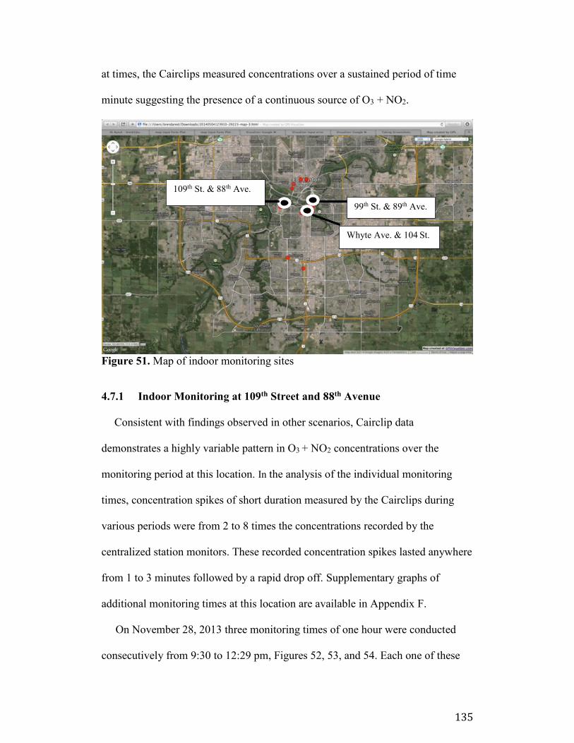
135
at times, the Cairclips measured concentrations over a sustained period of time
minute suggesting the presence of a continuous source of O3 + NO2.
Figure 51. Map of indoor monitoring sites
4.7.1 Indoor Monitoring at 109th Street and 88th Avenue
Consistent with findings observed in other scenarios, Cairclip data
demonstrates a highly variable pattern in O3 + NO2 concentrations over the
monitoring period at this location. In the analysis of the individual monitoring
times, concentration spikes of short duration measured by the Cairclips during
various periods were from 2 to 8 times the concentrations recorded by the
centralized station monitors. These recorded concentration spikes lasted anywhere
from 1 to 3 minutes followed by a rapid drop off. Supplementary graphs of
additional monitoring times at this location are available in Appendix F.
On November 28, 2013 three monitoring times of one hour were conducted
consecutively from 9:30 to 12:29 pm, Figures 52, 53, and 54. Each one of these
99th St. & 89th Ave.
Whyte Ave. & 104 St.
109th St. & 88th Ave.
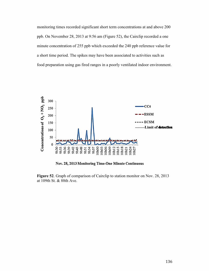
136
monitoring times recorded significant short term concentrations at and above 200
ppb. On November 28, 2013 at 9:56 am (Figure 52), the Cairclip recorded a one
minute concentration of 255 ppb which exceeded the 240 ppb reference value for
a short time period. The spikes may have been associated to activities such as
food preparation using gas fired ranges in a poorly ventilated indoor environment.
Figure 52. Graph of comparison of Cairclip to station monitor on Nov. 28, 2013
at 109th St. & 88th Ave.
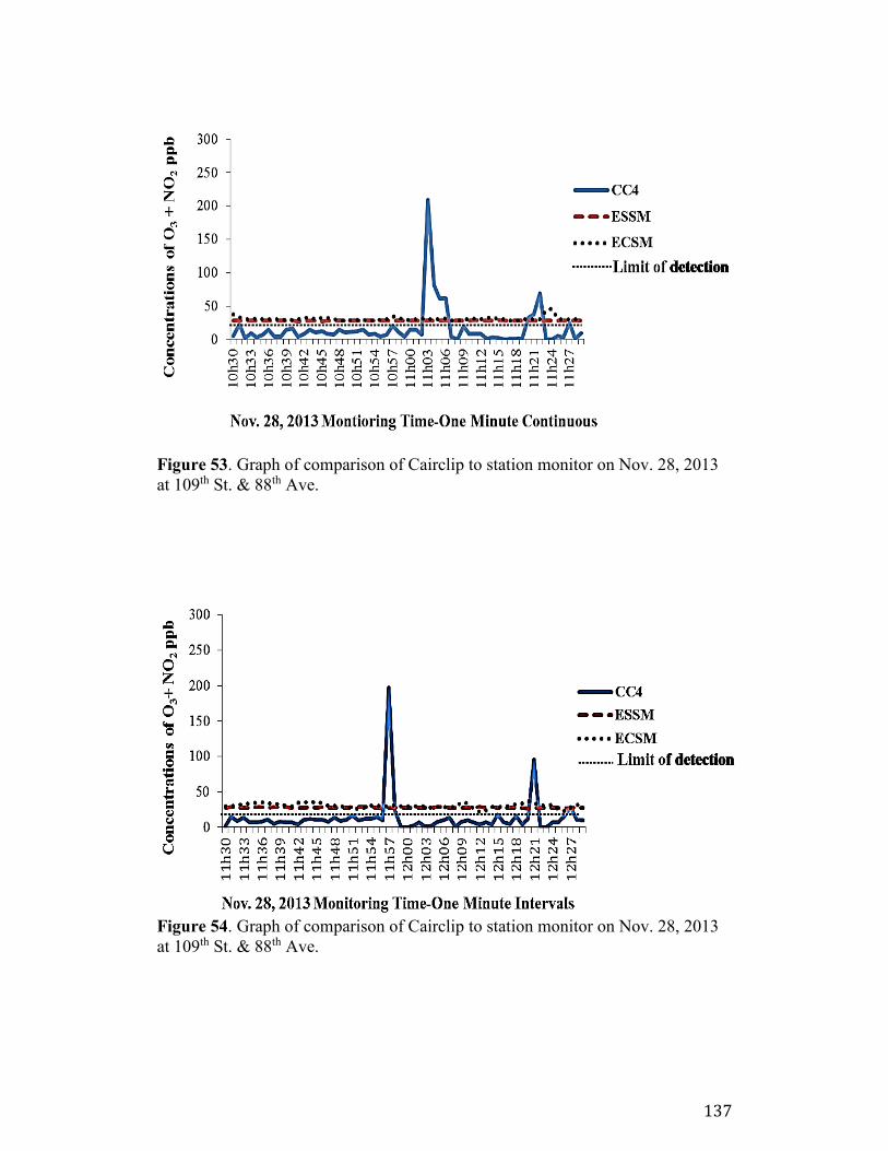
137
Figure 53. Graph of comparison of Cairclip to station monitor on Nov. 28, 2013
at 109th St. & 88th Ave.
Figure 54. Graph of comparison of Cairclip to station monitor on Nov. 28, 2013
at 109th St. & 88th Ave.
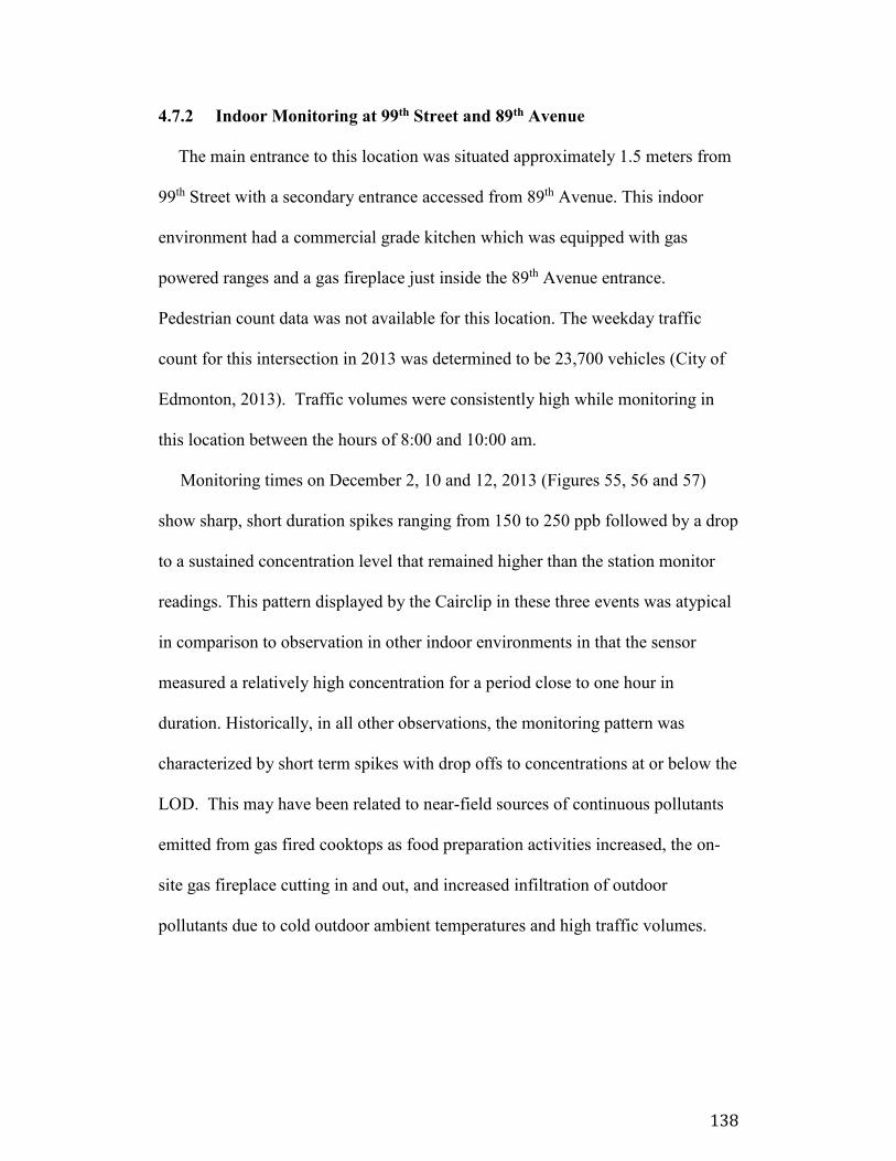
138
4.7.2 Indoor Monitoring at 99th Street and 89th Avenue
The main entrance to this location was situated approximately 1.5 meters from
99th Street with a secondary entrance accessed from 89th Avenue. This indoor
environment had a commercial grade kitchen which was equipped with gas
powered ranges and a gas fireplace just inside the 89th Avenue entrance.
Pedestrian count data was not available for this location. The weekday traffic
count for this intersection in 2013 was determined to be 23,700 vehicles (City of
Edmonton, 2013). Traffic volumes were consistently high while monitoring in
this location between the hours of 8:00 and 10:00 am.
Monitoring times on December 2, 10 and 12, 2013 (Figures 55, 56 and 57)
show sharp, short duration spikes ranging from 150 to 250 ppb followed by a drop
to a sustained concentration level that remained higher than the station monitor
readings. This pattern displayed by the Cairclip in these three events was atypical
in comparison to observation in other indoor environments in that the sensor
measured a relatively high concentration for a period close to one hour in
duration. Historically, in all other observations, the monitoring pattern was
characterized by short term spikes with drop offs to concentrations at or below the
LOD. This may have been related to near-field sources of continuous pollutants
emitted from gas fired cooktops as food preparation activities increased, the on-
site gas fireplace cutting in and out, and increased infiltration of outdoor
pollutants due to cold outdoor ambient temperatures and high traffic volumes.
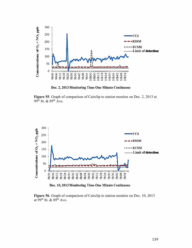
139
Figure 55. Graph of comparison of Cairclip to station monitor on Dec. 2, 2013 at
99th St. & 89th Ave.
Figure 56. Graph of comparison of Cairclip to station monitor on Dec. 10, 2013
at 99th St. & 89th Ave.
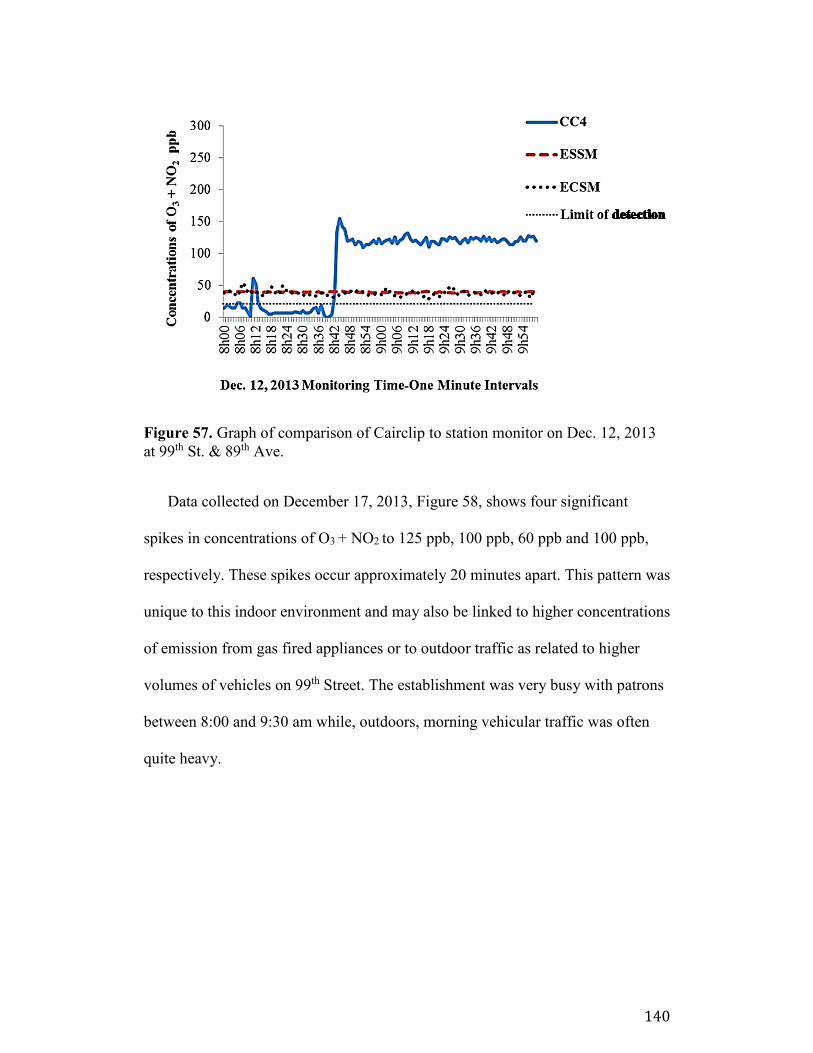
140
Figure 57. Graph of comparison of Cairclip to station monitor on Dec. 12, 2013
at 99th St. & 89th Ave.
Data collected on December 17, 2013, Figure 58, shows four significant
spikes in concentrations of O3 + NO2 to 125 ppb, 100 ppb, 60 ppb and 100 ppb,
respectively. These spikes occur approximately 20 minutes apart. This pattern was
unique to this indoor environment and may also be linked to higher concentrations
of emission from gas fired appliances or to outdoor traffic as related to higher
volumes of vehicles on 99th Street. The establishment was very busy with patrons
between 8:00 and 9:30 am while, outdoors, morning vehicular traffic was often
quite heavy.
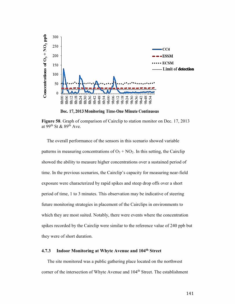
141
Figure 58. Graph of comparison of Cairclip to station monitor on Dec. 17, 2013
at 99th St & 89th Ave.
The overall performance of the sensors in this scenario showed variable
patterns in measuring concentrations of O3 + NO2. In this setting, the Cairclip
showed the ability to measure higher concentrations over a sustained period of
time. In the previous scenarios, the Cairclip’s capacity for measuring near-field
exposure were characterized by rapid spikes and steep drop offs over a short
period of time, 1 to 3 minutes. This observation may be indicative of steering
future monitoring strategies in placement of the Cairclips in environments to
which they are most suited. Notably, there were events where the concentration
spikes recorded by the Cairclip were similar to the reference value of 240 ppb but
they were of short duration.
4.7.3 Indoor Monitoring at Whyte Avenue and 104th Street
The site monitored was a public gathering place located on the northwest
corner of the intersection of Whyte Avenue and 104th Street. The establishment
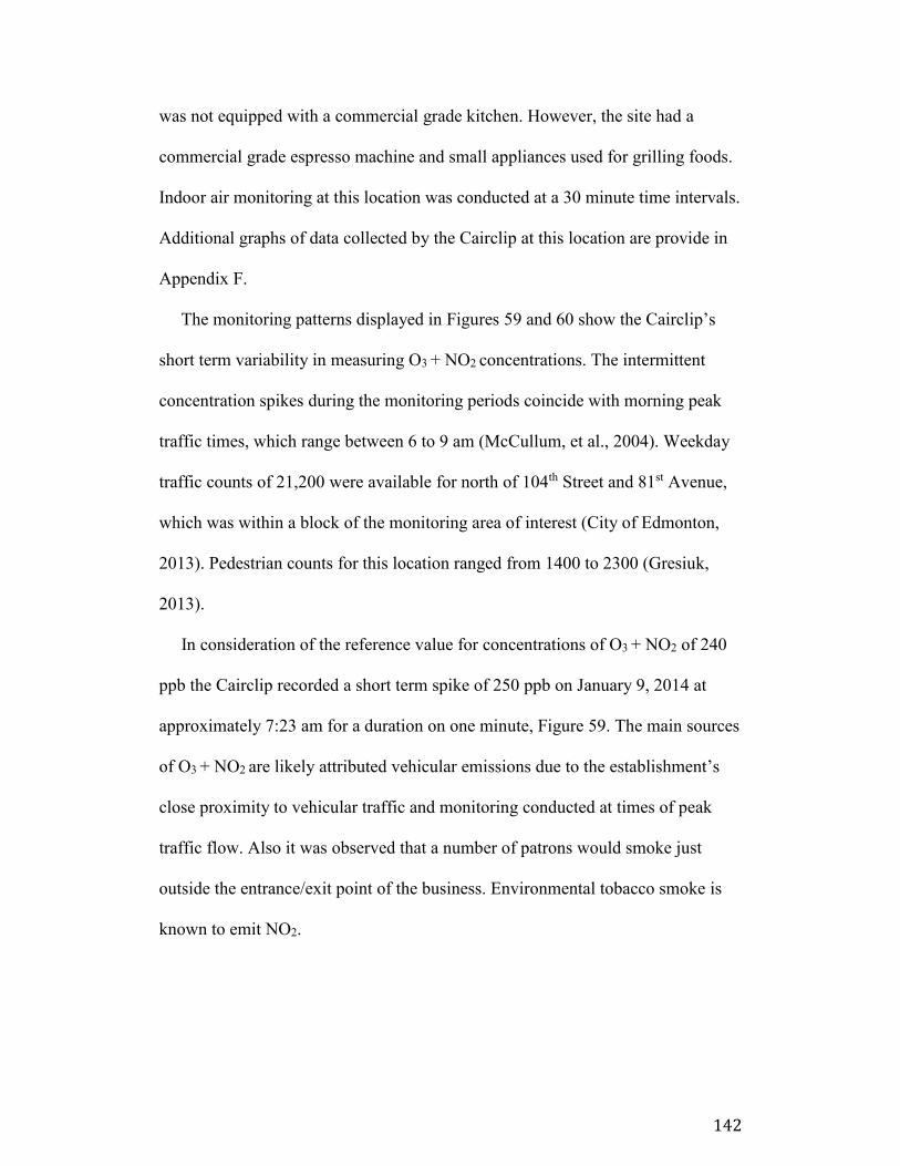
142
was not equipped with a commercial grade kitchen. However, the site had a
commercial grade espresso machine and small appliances used for grilling foods.
Indoor air monitoring at this location was conducted at a 30 minute time intervals.
Additional graphs of data collected by the Cairclip at this location are provide in
Appendix F.
The monitoring patterns displayed in Figures 59 and 60 show the Cairclip’s
short term variability in measuring O3 + NO2 concentrations. The intermittent
concentration spikes during the monitoring periods coincide with morning peak
traffic times, which range between 6 to 9 am (McCullum, et al., 2004). Weekday
traffic counts of 21,200 were available for north of 104th Street and 81st Avenue,
which was within a block of the monitoring area of interest (City of Edmonton,
2013). Pedestrian counts for this location ranged from 1400 to 2300 (Gresiuk,
2013).
In consideration of the reference value for concentrations of O3 + NO2 of 240
ppb the Cairclip recorded a short term spike of 250 ppb on January 9, 2014 at
approximately 7:23 am for a duration on one minute, Figure 59. The main sources
of O3 + NO2 are likely attributed vehicular emissions due to the establishment’s
close proximity to vehicular traffic and monitoring conducted at times of peak
traffic flow. Also it was observed that a number of patrons would smoke just
outside the entrance/exit point of the business. Environmental tobacco smoke is
known to emit NO2.
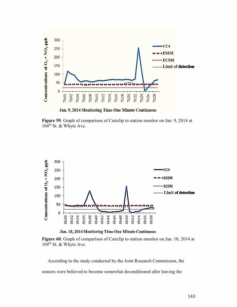
143
Figure 59. Graph of comparison of Cairclip to station monitor on Jan. 9, 2014 at
104th St. & Whyte Ave.
Figure 60. Graph of comparison of Cairclip to station monitor on Jan. 10, 2014 at
104th St. & Whyte Ave.
According to the study conducted by the Joint Research Commission, the
sensors were believed to become somewhat deconditioned after leaving the
144
factory where they are initially conditioned to detect O3 (Spinelle, 2013). In the
event that this deconditioning occurs, the sensitivity of the sensor decreases until
which time it is exposed to sufficient levels of O3. For this research, there is a
possibility that the sensors became deconditioned after leaving the factory and
that the concentrations that the sensors were exposed to during this study were not
high enough to recondition the sensors to an optimal level of sensitivity. This may
provide an explanation as to the sensors low O3 + NO2 concentration levels in
relation to both the NAPS station monitors and in real time scenarios where it is
was assumed the readings would be high.
As noted consistently throughout the study, the Cairclip’s monitoring
capabilities are designed to capture receptor-based exposure from a near-field
source. The Cairclip sensor is intended to represent measurements based on a real
time capacity which, in this study, was characterized with fluctuations in
concentrations of O3 + NO2 due to near-field sources.

145
5 CONCLUSIONS
The direction and focus of this research conducted using the Cairclip O3 + NO2
sensors was to provide evidence to support that air quality data recorded at
centralized fixed-site monitors, may not provide the best or most representative
information about individual personal exposures. While the Cairclips did not
perform as well as that dictated by the manufacturer when challenged against the
Edmonton south ambient monitoring station; they did provide valuable
information on short term concentration spikes during personal exposure
monitoring in various environments.
The Cairclips are designed to function in a similar capacity to that of the
centralized ambient monitoring stations; but differ in that the origin of the
pollutant sources are near-field and measured at the personal level. The
centralized monitors are large, expensive, non-portable, highly technical
instruments that are designed to measure pollutants on far-field source capacity.
In summary of phase one of the study, % RSD for the one hour, 30 and 15
minute averaged concentrations collected by paired Cairclips ranged from ±11 to
34%, ±12 to 39% and ±14 to 37%, respectively. The one hour averaged
concentrations presented the best comparative precision results, ±11 to 34%. The
summarized accuracy results for the one hour, 30 and 15 minute averaged
concentrations were as follows: ±29 to 43%; ±31 to 48 %; and, ±32 to 48%,
respectively. Again the one hour averaged concentrations showed the best
comparative accuracy results at a range between ±29 to 43%.
146
In summary of phase two monitoring of a residential environment, indoor
levels were consistently lower that outdoor concentrations. These findings can be
related to low production of indoor sources of O3 + NO2 and the scavenging
activities characteristic of these gases which lowers their concentrations (US
EPA, 2014a).
Findings during phase two monitoring of outdoor intersection sites in urban-
core environments demonstrated that the 97th and 109th Street location displayed
a greater variation with a number of concentration spikes ranging from 70 ppb to
200 ppb in comparison to the Jasper and 109th setting where concentration spikes
ranged from 40 ppb to 125 ppb, respectively. While the data from Whyte Avenue
and 109th Street displayed more frequent spikes of higher concentrations ranging
from 80 ppb to 120 ppb than levels measured at the Whyte Avenue and 99th
Street, which reached a one-time height of concentration at 100 ppb. The
intersections in the downtown core and the Whyte Avenue area were similar in
that several residential and commercial dwellings were located within close
proximity to vehicular traffic. As the monitoring at these intersections was
outdoor and within 2 meters of high traffic areas, the near-field source of O3 and
NO2 is mostly related to emissions from various types of vehicles.
The following are the important findings from phase two monitoring on public
transit via city bus and LRT. Peak concentrations on bus route #33 ranged from
60 ppb to 150 ppb. These concentrations were measured at various intervals on
route to West Edmonton Mall and when waiting inside and outside the bus at the
WEM transit station, respectively. During monitoring on LRT routes,
147
concentration spikes over the course of the entire monitoring period ranged from
50 ppb to 200 ppb. These spikes in O3 + NO2 measured were more commonly
observed during north-bound travel from Southgate to Grandin and in
underground LRT stations following train departure. The origin of these near-
field sources are most likely correlated to emissions from surrounding vehicular
traffic at transit stations and ambient concentrations that had infiltrated
underground the LRT passenger waiting areas.
Phase two findings from monitoring indoor non-residential locations displayed
concentration spikes of O3 + NO2 that ranged from 125 ppb to 250 ppb. The
following are the important findings from the three targeted locations are 1) the
locations of all three monitoring sites were in close proximity to high traffic
intersections with vehicular emission most likely the major contributor to near-
field sources; 2) the 109th Street /88th Avenue and the 99th Street /89th Avenue
locations were equipped with full commercial grade kitchens with gas-fired cook
tops, a potential source of pollutants; and 3) the Whyte Avenue and 104th Street
location often had several patrons smoking within close range of the front door,
environmental tobacco smoke (ETS) is a source of NO2, and; 4) the finding from
the 99th Street and 89th Avenue location were unique in that, at times, the
Cairclips measured an elevated concentration over a sustained period of time
indicating a continuous source of O3 + NO2.
Based on the results of this study, the efficacy of the Cairclip O3 + NO2 sensor
is questionable in environments where concentrations of O3 and NO2 are relatively
low such as that in urban Edmonton. Consideration must be given to the fact that
148
the sensors are both manufactured and tested in Europe, specifically France,
where geographical, climatic, and emission conditions are quite different from
that of Edmonton.
Because the sensors measure a sum concentration of O3 and NO2 it is
difficult to determine the independent levels of each gas. As the monitoring
period extended from mid-September to late December, 2013 and the Cairclip is
thought to have a higher sensitivity to NO2 (Spinnelle, 2013), it is most likely that
higher levels of NO2 were recorded. Ozone is characteristically known to be more
abundant in summer months when ambient temperatures are high with ample UV
light exposure (Alberta Environment, 2013c). Finally, any significant spikes in
concentrations of O3 + NO2 measured by the Cairclips during these monitoring
times ranged from just one to three minutes with levels mostly below the
reference value of 240 ppb.
As this research provides a baseline for understanding the capabilities and
limitations of new technology in air monitoring, further studies in various
microenvironments may be advantageous. In this study, the Cairclip sensors
displayed interesting results when tested on public transit and when placed in
indoor commercial environments. Further studies using the Cairclips in similar
settings to these may prove to be advantageous in gaining further knowledge of
receptor-based exposure of short duration to near-field sources. Prior to further
monitoring in these locations, it may be advantageous to replace the micro-filter
and lithium-ion battery as suggested by the manufacturers. Upon which time, the

149
accuracy and precision of these sensors be re-tested prior to further use in
personal monitoring research.
150
6 REFERENCES
Adams, C., Riggs, P., and Volckens, J. (2009). Development of a method for
personal, spatiotemporal exposure assessment. Journal of Environmental
Monitoring : JEM, 11(7), 1331–9. doi:10.1039/b903841h
Alberta Capital Air Shed. (2014). Alberta Environment. Retrieved from
http://www.capitalairshed.ca
Alberta Environment. (2012a). Clearing the air Alberta’s renewed clean air
strategy. Retrieved from http://esrd.alberta.ca/air/documents/8692.pdf
Alberta Environment. (2014b). Particulate matter and ozone – progess towards
meeting the Canada-wide standards. Retrieved from
http://www.environment.alberta.ca/02833.html
Alberta Environment. (2013c). South Saskatchewan region air quality
management framework for nitrogen dioxide, ozone and fine particulate
matter. Retrieved from http://environmentuat.alberta.ca/documents/SSRP-
AirQualityManagement-Draft-Oct10-2013.pdf
Alberta Environment. (2009d). Air management in Alberta. Retrieved from
http://environment.gov.ab.ca/info/library/8137.pdf
Alberta Environment. (2006e). Guidelines for quality assurance and quality
control in surface water quality programs in Alberta. Retrieved from
http://www.environment.gov.ab.ca/info/library/7739.pdf
Berman, J. D., Fann, N., Hollingsworth, J. W., Pinkerton, K. E., Rom, W. N.,
Szema, A. M., Breysse, P. N., White, R. H., and Curriero, F. C. (2012).
Health benefits from large-scale ozone reduction in the United States.
Environmental Health Perspectives, 120(10), 1404–10.
doi:10.1289/ehp.1104851
Bradley, M. J. and Jones, B. M. (2002). Reducing Global NO x Emissions:
Developing Advanced Energy and Transportation Technologies. AMBIO: A
Journal of the Human Environment, 31(2), 141–149. doi:10.1579/0044-
7447-31.2.141
Cairpol. (2014). Retrieved from: www.cairpol.com
Carvalho, V., Lopes, J. G., Ramos, H. G., and Correa Alegria, F. (2009). City-
wide mobile air quality measurement system. Sensors, 2009 IEEE, 546-551.
doi: 10.1109/ICSENS.2009.5398299

151
Cazorla, M., Brune, W. H., Ren, X., and Lefer, B. (2012). Direct measurement of
ozone production rates in Houston in 2009 and comparison with two
estimation methods. Atmospheric Chemistry and Physics, 12(2), 1203–1212.
doi:10.5194/acp-12-1203-2012
Chan, C. Y., Chan, L. Y., and Harris, J. M. (2003). Urban and background ozone
trend in 1984-1999 at subtropical Hong Kong, South China. Ozone
Engineering and Science. Retrieved from
http://web.ebscohost.com.login.ezproxy.library.ualberta.ca/ehost/pdfviewer/
pdfviewer?sid=adc4e102-a5f8-449c-b869-
992e56edec80%40sessionmgr15&vid=2&hid=11
City of Edmonton. (2014a). Air quality. Retrieved from
http://www.edmonton.ca/environmental/programs/air-quality.aspx - Air
Quality: City of Edmonton
City of Edmonton. (2014b). Traffic volumes and turning movements : City of
Edmonton. Retrieved from
http://www.edmonton.ca/transportation/traffic_reports/traffic-volumes-
turning-movements.aspx
Clean Air Strategic Alliance (CASA). (2014). Retrieved from
http://www.casadata.org/Report/DataReports/Stationinformation.aspx?Param
eter/=01&Parameter2=043
Curran, R. L. T., Guigard, S. E., and Kindzierski, W. B. (2012). Analysis of the
field accuracy and precision of passive monitors for ambient SO2, NO2 and
O3 in Alberta. Air and Waste Management Association. Retrieved from
http://www.meetingproceedings.us/2012/awma/contents/papers/34.pdf
Currie, L. A., and Svehla, G. (1994). Nomenclature for the presentation of results
of chemical analysis. Pure & Applied Chemistry, 66(3), 595–608.
Demokritou, P., Kavouras, I. G., Ferguson, S. T., and Koutrakis, P. (2001).
Development and laboratory performance evaluation of a personal
multipollutant sampler for simultaneous measurements of particulate and
gaseous pollutants. Aerosol Science and Technology, 35(3), 741–752.
doi:10.1080/02786820152546789
Environment Canada. (2005a). Air - Can-US air quality agreement. Retrieved
from https://www.ec.gc.ca/Air/default.asp?lang=En&n=1E841873-1
Environment Canada. (2013b). Ambient air quality standards for specific criteria
contaminants. Retrieved from http://www.hc-sc.gc.ca/ewh-semt/air/out-
ext/reg-eng.php#a2-RegulationsRealtedtoHealth+AirQuality
152
Environment Canada. (2013c). National air pollution surveillance network
(NAPS). Retrieved from
ec.gc.ca.natchem/default.asp?lang=En&n=EEOE2169-E42E-46C7-8571
European Commission. (2014a). Air quality standards - Environment - European
Commission. Retrieved from
http://ec.europa.eu/environment/air/quality/standards.htm
European Commission. (2008b). Directive 2008/50/EC of the European
Parliament and of the Council of 21 May 2008 on ambient air quality and
cleaner air for Europe. Official Journal of the European Union. Retrieved
from http://eur-lex.europa.eu/legal-
content/EN/TXT/HTML/?uri=OJ:L:2008:152:FULL&from=EN
Fenske, R. (2010). For good measure: Origins and prospects of exposure science
(2007 Wesolowsk Award Lecture). Journal of Exposure Science &
Environmental Epidemiology. doi:10, 1038/jes.2010.26. Epub 2010 Apr 28
Fort Air Partnership. (2014). How is air quality monitored. Government of
Alberta. Retrieved from http://www.fortair.org
Gaga, E. O., Döğeroğlu, T., Ozden, O., Ari, A., Yay, O. D., Altuğ, H., Akyol, N.,
Ornektekin, S., and Van Doorn, W. (2012). Evaluation of air quality by
passive and active sampling in an urban city in Turkey: current status and
spatial analysis of air pollution exposure. Environmental Science and
Pollution Research International, 19(8), 3579–96. doi:10.1007/s11356-012-
0924-y
Geyh, A. S., Wolfson, J. M., Koutrakis, P., Mulik, J. D., and Avol, E. L. (1997).
Development and evaluation of a small active ozone sampler. Environmental
Science & Technology, 31(8), 2326–2330. doi:10.1021/es960945+
Gilbert, N., Woodhouse, S., Stieb, D. and Brook, J. (2003). Ambient nitrogen
dioxide and distance from a major roadway. Science and the Total
Environment. 312(1-3) 43-46. Retrieved from
http://www.sciencedirect.com/science/article/pii/S0048969703002286
Gresiuk, M. (2013). Sticks and stones: Pedestrian counting. Responsible
Hospitality Edmonton. Retrieved from
http://www.responsiblehospitalityedmonton.ca/wp-
content/uploads/2013/08/RHE-13-Pedestrian-Counts-Whyte-V.2.pdf

153
Gwinn, M. R., Craig, J., Axelrad, D. A., Cook, R., Dockins, C., Fann, N., Fegley,
R., Guinnup, D. E., Helfand, G., Hubbell, B., Mazur, S. L., Palma, T., Smith,
R. L., Vandeberg, J. and Sonawane, B. (2011). Meeting report: Estimating
the benefits of reducing hazardous air pollutants--summary of 2009
workshop and future considerations. Environmental Health Perspectives,
119(1), 125–30. doi:10.1289/ehp.1002468
Harris, J. L. (2013). Reducing biological pollutants in household living areas -
Indoor air quality. Retrieved from
http://fcs.tamu.edu/housing/healthy_homes/indoor_air_quality/biological_po
llutants/reducing_biological_pollutants.php
Itahashi, S., Uno, I., and Kim, S. (2013). Seasonal source contributions of
tropospheric ozone over East Asia based on CMAQ–HDDM. Atmospheric
Environment, 70, 204–217. doi:10.1016/j.atmosenv.2013.01.026
Johnson, J. Y. M., Rowe, B. H, Allen, P. A., and Villeneuve, P. J. (2013). A case-
control study of medium-term exposure to ambient nitrogen dioxide
pollution and hospitalization for stroke. BMC Public Health, 13(368), 1–9.
Retrieved from http://www.biomedcentral.com/147-2458/13/368
Kindzierski, W., Guigard, S., Schulz, J., Vidmar, J., and Purthill, C. (2007).
Reference assessment report on Nitrogen Dioxide for developing ambient air
quality objectives. Alberta Environment. Retrieved from
http://www.environment.gov.ab.ca/info/library/8302.pdf
Kindzierski, W. (2013). Personal exposure monitoring, lecture notes distributed in
Exposure Assessment 511 at the University of Alberta, Edmonton in
September, 2013.
Koehler, C., Thielen, S., Ginzkey, C., Hackenberg, S., Scherzed, A., Burghartz,
M., Paulus, R.H., and Kleinsasser, N. H. (2013). Nitrogen dioxide is
genotoxic in urban concentrations. Inhalation Toxicology, 25(6), 341–7.
doi:10.3109/08958378.2013.788104
Krupa, S. V and Legge, A. H. (2000). ScienceDirect.com - Environmental
pollution - Passive sampling of ambient, gaseous air pollutants: an
assessment from an ecological perspective. Science Direct, 107 (1), 31–45.
doi: 10.1016/S0269-749(99) 001. Retrieved from
http://www.sciencedirect.com.login.ezproxy.library.ualberta.ca/science/articl
e/pii/S0269749199001542
Labelle, C. (1998). Effects of ozone, sulphates, and particulate matter on health.
Parliamentary Research Branch Health Canada. Retrieved from
http://www.publications.gc.ca/Collection-R/LoBdP/modules/prb98-4-
smog/effectsofozone-e.htm.

154
Lin, C., Becker, S., Timmis, R., and Jones, K. C. (2011). A new through-flow
directional passive air sampler: design, performance and laboratory testing
for monitoring ambient nitrogen dioxide. Atmospheric Pollution Research,
2(1), 1–8. doi:10.5094/APR.2011.001.
Lioy, P. J. (2010). Exposure science: a view of the past and milestones for the
future. Environmental Health Perspectives, 118(8), 1081–90.
doi:10.1289/ehp.0901634. Retrieved from
http://www.pubmedcentral.ncbi.nlm.nih.gov/pmc/articles/PMC2920079
McCullum, K., Hahsam, F. and Kindzierski, W. (2004). Ambient air quality
trends using data collected throughout Alberta. Air and Waste Management
Association 97th Annual Conference and Exhibition (ACE), 1-15.
Indianapolis, IN.
Mendenhal, W. and Sincich, T. (1995). Statistics for engineering and the
sciences, (4th ed.). Engelwood Cliffs, NJ: Prentice Hall.
Minitab Inc. (2010). Regression analysis. Retrieved from http://www.minitab.com
Montgomery, D. C. (2009). Design and analysis of experiments, (7th ed.).
Hoboken, NJ: John Wiley & Sons.
Mukerjee, S., Smith, L. A, Norris, G. A, Morandi, M. T., Gonzales, M., Noble, C.
A., Neas, L. M., and Ozkaynak, A. H. (2004). Field method comparison
between passive air samplers and continuous monitors for VOCs and NO2 in
El Paso, Texas. Journal of the Air & Waste Management Association, 54(3),
307–19. Retrieved from http://www.ncbi.nlm.nih.gov/pubmed/15068008
National Academy of Sciences. (1977). A report to the U. S. Environmental
Protection Agency from the Study Group on Environmental Monitoring,
Committee on National Statistics, National Research Council. National
Academy of Sciences, Washington, DC
National Library of Medicine. (2013). Tox town - Nitrogen oxides - Toxic
chemicals and environmental health risks where you live and work - Text
version. Retrieved from
http://toxtown.nlm.nih.gov/text_version/chemicals.php?id=19
National Research Council (US). (1991). Human exposure assessment for
airborne pollutants: Advances and opportunities. National Academy Press.
Retrieved from http://www. nap.edu.catalogu/1544.html
155
Nejadkoorki, F., Nicholson, K., and Hadad, K. (2011). The design of long-term
air quality monitoring networks in urban areas using a spatiotemporal
approach. Environmental Monitoring and Assessment, 172(1-4), 215–23.
doi:10.1007/s10661-010-1328-4
Ojima, J. (2012). Gaseous contaminant distribution in the breathing zone.
Industrial Health, 50(3), 236–8. Retrieved from
http://www.ncbi.nlm.nih.gov/pubmed/22790482
O’Neill, M. S., Jerrett, M., Kawachi, I., Levy, J .I., Choen, A. J., Gouveia, N.,
Wilkinson, P., Fletcher, T., Cifuentes, L. and Schwartz, J. (2003). Health
wealth and air pollution. Environmental Health Perspectives, 111(16), 1861-
70. Retrieved from
http://web.b.ebscohost.com.login.eproxy.library.ualberta.ca
Ozkaynak, H., Baxter, L. K., Dionisio, K. L., and Burke, J. (2013). Air pollution
exposure prediction approaches used in air pollution epidemiology studies.
Journal of Exposure Science & Environmental Epidemiology.
doi:10.1038/jes.2013.15
Ott, W. R., Steinemann A. C., and Wallace, L. A. (2007) Exposure analysis: A
receptor-oriented science. Boca Raton, FL: Taylor and Francis Group.
Ott, W. R. (1985b). Total human exposure. Environmental Science & Technology,
19(10), 880–886.
Prabamroong, T., Manomaiphiboon, K., Limpaseni, W., Sukhapan, J., and
Bonnet, S. (2012). Ozone and its potential control strategy for Chon Buri
city, Thailand. Journal of the Air & Waste Management Association, 62(12),
1411–1422. doi:10.1080/10962247.2012.716385
Ray, J. D. (2001). Spatial distribution of tropospheric ozone in National Parks of
California: Interpretation of passive sampler data. In proceedings of the
International Symposium of Gasious Air Pollutants in Ecological Effects
Research. The Scientific World Journal, 1, 483–497.
doi:10.1100/tsw.2001.83
Ryan, P. B., Soczek, M. Lou, Treitman, R. D., Spengler, J. D., and Billick, I. H.
(1988). The Boston residential NO2 characterization study—II. Survey
methodology and population concentration estimates. Atmospheric
Environment (1967), 22(10), 2115–2125. doi:10.1016/0004-6981(88)90123-
0

156
Sandell, M. (1998). Putting NOx in a box - ProQuest. Pollution Engineering,
30(3), 56–58. Retrieved from
http://search.proquest.com.login.ezproxy.library.ualberta/ca/docview/220983
405?aCCounted=14474
Sherwood, R. J., and Greenhalgh, D. M. S (1960). A personal sampler. Annals of
Occupational Hygiene, 2, 127–32.
Spaeth, K. (2000). Winner of the 1999 best medical student paper in preventive
medicine: Don’t hold your breath: Personal exposures to volatile organic
compounds and other toxins in indoor air and what's (not) being done about
it. Science Direct Preventative Medicine, 31(6), 631-37. Retrieved from
http://www.sciencedirect.com.login.ezproxy.library.ualberta.ca/science/articl
e/pii/S0091743500907692
Spengler, J. D. and Soczek, M. L., (1984). Evidence for improved ambient air
quality and the need for personal exposure research. Environmental Science
and Technology, 18(9), 268A–80A. Retrieved from
http://www.searchproquest.com.login.ezproxy.library.ualberta.ca/pollution/d
ocview/14003399/abstract/13EE18D006061B5CA6A/2?aCCountid=14474
Spinnelle, L., Gerboles, M., and Aleixandre, M. (2013). Report of laboratory and
in-situ validation of micro-sensor for monitoring ambient air pollution. Joint
Research Center Technical Reports, 1-59. doi: 10.2788/4277. Retrieved
from: http://www.jrc.ec.europa.eu/
Steinle, S., Reis, S., and Sabel, C. E. (2013). Quantifying human exposure to air
pollution--moving from static monitoring to spatio-temporally resolved
personal exposure assessment. The Science of the Total Environment, 443,
184–93. doi:10.1016/j.scitotenv.2012.10.098
US Environmental Protection Agency (US EPA). (2014a). Nitrogen dioxide
implementation-Program and requirements for reducing oxides of nitrogen.
Retrieved from
http://www.epa.gov/airquality/nitrogenoxides/implement.html
US Environmental Protection Agency (US EPA). (2014b). Health | Nitrogen
Dioxide | Ozone. Retrieved from
http://www.epa.gov/oaqps001/nitrogenoxides/health.html
US Environmental Protection Agency (US EPA). (2012c). Fact sheet: Final
revisions to the secondary national ambient air quality standards for oxides
of nitrogen and sulfur. 2 : 0.053 (pp. 1–4). Retrieved from
20120320factsheet.pdf

157
US Environmental Protection Agency (US EPA). (2014d). Scientists evaluate air
sensors developed during EPA’s air sensor evaluation and collaboration
event. Retrieved from http://www.epa.gov/nerl/features/sensors.html
US Environmental Protection Agency (US EPA). (2014e). Near roadway air
pollution and health. Retrieved from
http://www.epa.gov/otaq/nearroadway.htm
Wallace, L. A., and Ott, W. R. (1982). Personal monitors: A state-of-the-art
survey. Journal of the Air Pollution Control Association, 32(6), 601–610.
doi:10.1080/00022470.1982.10465435
Wallace, L. A. (2007a). Personal monitors. Exposure analysis. Boca Raton:
Taylor & Francis, 99-112.
Wallace, L.A. (1987b). The total exposure assessment methodology (TEAM)
study: Summary and analysis, volume 1. Washington, DC. EPA 600/S6–
97/002a. Retrieved from http://exposurescience-
org/pub/reports/TEAM_Study_book_1987.pdf
Wood Buffalo Environmental Association (WBEA) (2008). Human exposure
monitoring program monitoring year results. Retrieved from
www.health.alberta.ca/documents/WBEA-HEMP-2006-Technical.pdf
World Health Organization. (2005a). Air quality guidelines for particulate matter,
ozone, nitrogen dioxide and sulfur dioxide. (2005), 1–22. Retrieved from
http://www.who.int/phe/health_topics/outdoorair/outdoorair_aqg/en/
World Health Organization. (2003b). Health aspects of air pollution with
particulate matter, ozone and nitrogen dioxide, (January), 1–94. Retrieved
from www.euro.who.int/_data/assets/pdf_file/0005/112199/E79097.pdf
World Health Organization. (2000c). Effects of airborne nitrogen pollutants. Air
Quality Guidelines, 2 (14). Retrieved from
http://www.euro.who.int/__data/assets/pdf_file/0008/123101/AQG2ndEd_14n
itrogenload.pdf
Yoshida, K., and Kasama, K. (1987). Biotransformation of nitric oxide.
Environmental Health Perspectives, 73, 201–5. Retrieved from
http://www.pubmedcentral.nih.gov/articlerender.fcgi?artid=1474568&tool=p
mcentrez&rendertype=abstract
Yu, C. H., Morandi, M. T., and Weisel, C. P. (2008). Passive dosimeters for
nitrogen dioxide in personal/indoor air sampling: a review. Journal of
Exposure Science & Environmental Epidemiology, 18(5), 441–51.
doi:10.1038/jes.2008.22
158
Yusa, V., Coseolla, C., Mellouki, W., Pastor, A., and de la Guardia, M. (2009).
Journal of chromatography: A sampling and analysis of pesticides in ambient
air. Science Direct, 1216(15), 2972-2983. Retrieved from
http://www.sciencedirect.com/science/article/pii/S0021967309002283
Zhang, J. J., and Lioy, P. J. (2002). Human exposure assessment in air pollution
systems. The Scientific World Journal, 2, 497–513.
doi:10.1100/tsw.2002.119
Zhang, Y., Bocquet, M., Mallet, V., Seigneur, C., and Baklanov, A. (2012). Real-
time air quality forecasting, part I: History, techniques, and current status.
Atmospheric Environment, 60, 632–655.
doi:10.1016/j.atmosenv.2012.06.031
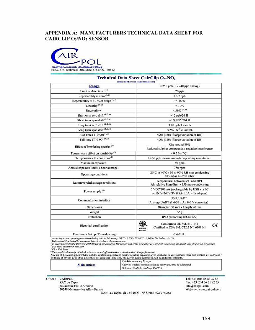
159
APPENDIX A: MANUFACTURERS TECHNICAL DATA SHEET FOR
CAIRCLIP O3/NO2 SENSOR

160
APPENDIX B: SIGN IN SHEET FOR ENTRANCE AND EXIT INTO THE
EDMONTON SOUTH STATION MONITOR
Sign in Sheet
entry and exit of
Station Monitor
Edmonton south
Date:
Time in: AM or
PM
Time Out: AM or
PM
Conditions or
comments
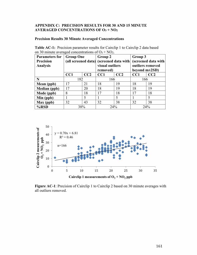
161
APPENDIX C: PRECISION RESULTS FOR 30 AND 15 MINUTE
AVERAGED CONCENTRATIONS OF O3 + NO2
Precision Results 30 Minute Averaged Concentrations
Table AC-1: Precision parameter results for Cairclip 1 to Cairclip 2 data based
on 30 minute averaged concentrations of O3 + NO2.
Parameters for
Precision
Analysis
Group One
(all screened data)
Group 2
(screened data with
visual outliers
removed)
Group 3
(screened data with
outliers removed
beyond m±2SD)
CC1 CC2 CC1 CC2 CC1 CC2
N 182 166 166
Mean (ppb) 17 21 18 19 18 19
Median (ppb) 17 20 18 19 18 19
Mode (ppb) 8 18 17 18 17 18
Min (ppb) 1 5 1 5 1 5
Max (ppb) 32 43 32 38 32 38
%RSD 38% 24% 24%
Figure AC-1: Precision of Cairclip 1 to Cairclip 2 based on 30 minute averages with
all outliers removed.
y = 0.70x + 6.81
R² = 0.46
0
10
20
30
40
50
0 5 10 15 20 25 30 35
Cair
clip
2 m
eau
rem
ents
of
O3
+ N
O2
p
pb
Cairclip 1 measurements of O3 + NO2 ppb
n=166
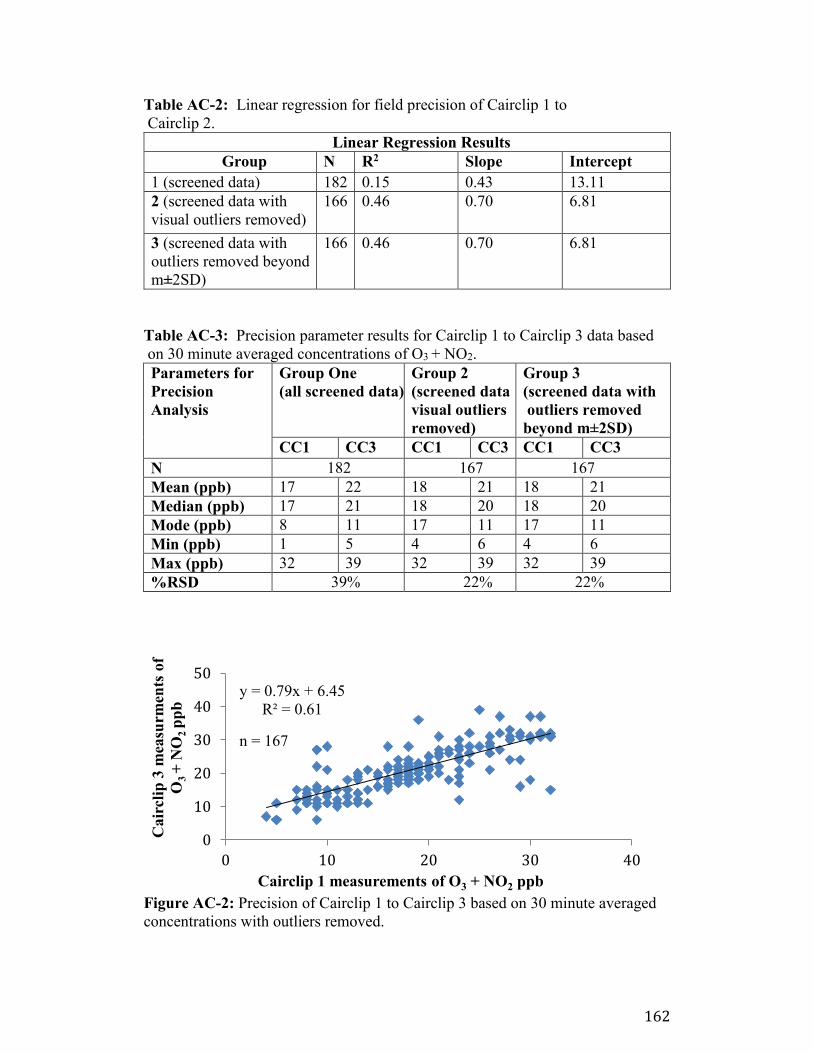
162
Table AC-2: Linear regression for field precision of Cairclip 1 to
Cairclip 2.
Linear Regression Results
Group N R2 Slope Intercept
1 (screened data) 182 0.15 0.43 13.11
2 (screened data with
visual outliers removed)
166 0.46 0.70 6.81
3 (screened data with
outliers removed beyond
m±2SD)
166 0.46 0.70 6.81
Table AC-3: Precision parameter results for Cairclip 1 to Cairclip 3 data based
on 30 minute averaged concentrations of O3 + NO2.
Parameters for
Precision
Analysis
Group One
(all screened data)
Group 2
(screened data
visual outliers
removed)
Group 3
(screened data with
outliers removed
beyond m±2SD)
CC1 CC3 CC1 CC3 CC1 CC3
N 182 167 167
Mean (ppb) 17 22 18 21 18 21
Median (ppb) 17 21 18 20 18 20
Mode (ppb) 8 11 17 11 17 11
Min (ppb) 1 5 4 6 4 6
Max (ppb) 32 39 32 39 32 39
%RSD 39% 22% 22%
Figure AC-2: Precision of Cairclip 1 to Cairclip 3 based on 30 minute averaged
concentrations with outliers removed.
y = 0.79x + 6.45
R² = 0.61
0
10
20
30
40
50
0 10 20 30 40
Cair
clip
3 m
easu
rmen
ts o
f
O3
+ N
O2
pp
b
Cairclip 1 measurements of O3 + NO2 ppb
n = 167
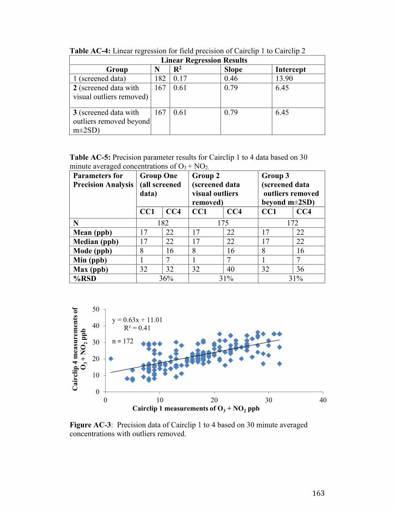
163
Table AC-4: Linear regression for field precision of Cairclip 1 to Cairclip 2
Linear Regression Results
Group N R2 Slope Intercept
1 (screened data) 182 0.17 0.46 13.90
2 (screened data with
visual outliers removed)
167 0.61 0.79 6.45
3 (screened data with
outliers removed beyond
m±2SD)
167 0.61 0.79 6.45
Table AC-5: Precision parameter results for Cairclip 1 to 4 data based on 30
minute averaged concentrations of O3 + NO2.
Parameters for
Precision Analysis
Group One
(all screened
data)
Group 2
(screened data
visual outliers
removed)
Group 3
(screened data
outliers removed
beyond m±2SD)
CC1 CC4 CC1 CC4 CC1 CC4
N 182 175 172
Mean (ppb) 17 22 17 22 17 22
Median (ppb) 17 22 17 22 17 22
Mode (ppb) 8 16 8 16 8 16
Min (ppb) 1 7 1 7 1 7
Max (ppb) 32 32 32 40 32 36
%RSD 36% 31% 31%
Figure AC-3: Precision data of Cairclip 1 to 4 based on 30 minute averaged
concentrations with outliers removed.
y = 0.63x + 11.01
R² = 0.41
0
10
20
30
40
50
0 10 20 30 40
Cair
clip
4 m
easu
rem
ents
of
O3
+ N
O2
pp
b
Cairclip 1 measurements of O3 + NO2 ppb
n = 172
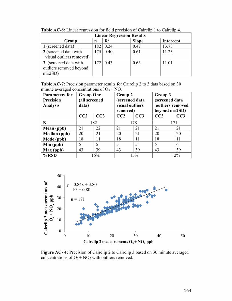
164
Table AC-6: Linear regression for field precision of Cairclip 1 to Cairclip 4.
Linear Regression Results
Group n R2 Slope Intercept
1 (screened data) 182 0.24 0.47 13.73
2 (screened data with
visual outliers removed)
175 0.40 0.61 11.23
3 (screened data with
outliers removed beyond
m±2SD)
172 0.43 0.63 11.01
Table AC-7: Precision parameter results for Cairclip 2 to 3 data based on 30
minute averaged concentrations of O3 + NO2.
Parameters for
Precision
Analysis
Group One
(all screened
data)
Group 2
(screened data
visual outliers
removed)
Group 3
(screened data
outliers removed
beyond m±2SD)
CC2 CC3 CC2 CC3 CC2 CC3
N 182 178 171
Mean (ppb) 21 22 21 21 21 21
Median (ppb) 20 21 20 21 20 20
Mode (ppb) 18 11 18 11 18 11
Min (ppb) 5 5 5 5 5 6
Max (ppb) 43 39 43 39 43 39
%RSD 16% 15% 12%
Figure AC- 4: Precision of Cairclip 2 to Cairclip 3 based on 30 minute averaged
concentrations of O3 + NO2 with outliers removed.
y = 0.84x + 3.80
R² = 0.80
0
10
20
30
40
50
0 10 20 30 40 50
Cair
clip
3 m
easu
rem
ents
of
O3
+ N
O2
pp
b
Cairclip 2 measurements O3 + NO2 ppb
n = 171
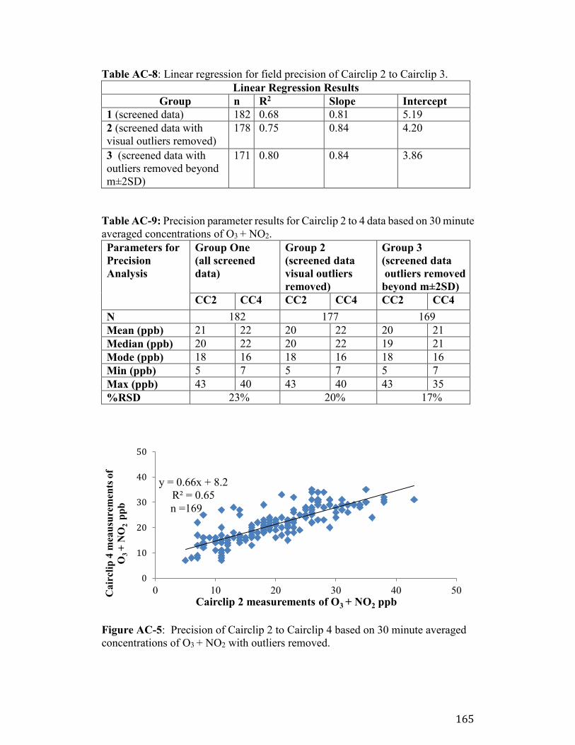
165
Table AC-8: Linear regression for field precision of Cairclip 2 to Cairclip 3.
Linear Regression Results
Group n R2 Slope Intercept
1 (screened data) 182 0.68 0.81 5.19
2 (screened data with
visual outliers removed)
178 0.75 0.84 4.20
3 (screened data with
outliers removed beyond
m±2SD)
171 0.80 0.84 3.86
Table AC-9: Precision parameter results for Cairclip 2 to 4 data based on 30 minute
averaged concentrations of O3 + NO2.
Parameters for
Precision
Analysis
Group One
(all screened
data)
Group 2
(screened data
visual outliers
removed)
Group 3
(screened data
outliers removed
beyond m±2SD)
CC2 CC4 CC2 CC4 CC2 CC4
N 182 177 169
Mean (ppb) 21 22 20 22 20 21
Median (ppb) 20 22 20 22 19 21
Mode (ppb) 18 16 18 16 18 16
Min (ppb) 5 7 5 7 5 7
Max (ppb) 43 40 43 40 43 35
%RSD 23% 20% 17%
Figure AC-5: Precision of Cairclip 2 to Cairclip 4 based on 30 minute averaged
concentrations of O3 + NO2 with outliers removed.
y = 0.66x + 8.2
R² = 0.65
0
10
20
30
40
50
0 10 20 30 40 50Cair
clip
4 m
eau
sure
men
ts o
f
O3
+ N
O2
p
pb
Cairclip 2 measurements of O3 + NO2 ppb
n =169
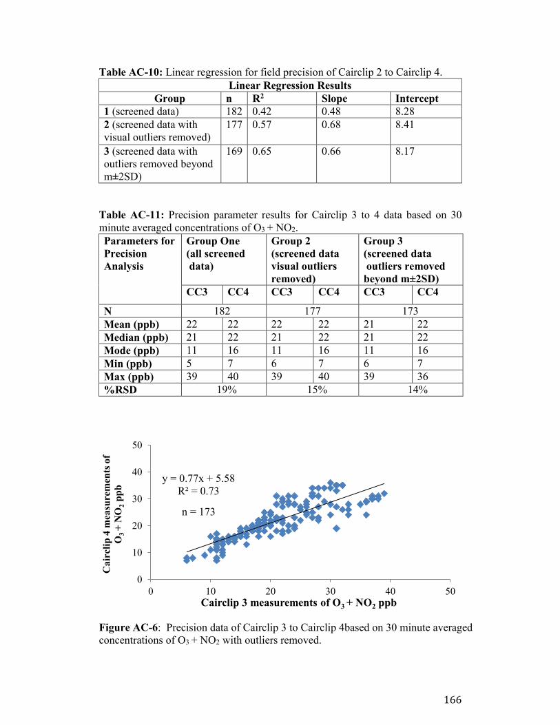
166
Table AC-10: Linear regression for field precision of Cairclip 2 to Cairclip 4.
Linear Regression Results
Group n R2 Slope Intercept
1 (screened data) 182 0.42 0.48 8.28
2 (screened data with
visual outliers removed)
177 0.57 0.68 8.41
3 (screened data with
outliers removed beyond
m±2SD)
169 0.65 0.66 8.17
Table AC-11: Precision parameter results for Cairclip 3 to 4 data based on 30
minute averaged concentrations of O3 + NO2.
Parameters for
Precision
Analysis
Group One
(all screened
data)
Group 2
(screened data
visual outliers
removed)
Group 3
(screened data
outliers removed
beyond m±2SD)
CC3 CC4 CC3 CC4 CC3 CC4
N 182 177 173
Mean (ppb) 22 22 22 22 21 22
Median (ppb) 21 22 21 22 21 22
Mode (ppb) 11 16 11 16 11 16
Min (ppb) 5 7 6 7 6 7
Max (ppb) 39 40 39 40 39 36
%RSD 19% 15% 14%
Figure AC-6: Precision data of Cairclip 3 to Cairclip 4based on 30 minute averaged
concentrations of O3 + NO2 with outliers removed.
y = 0.77x + 5.58
R² = 0.73
0
10
20
30
40
50
0 10 20 30 40 50
Cair
clip
4 m
easu
rem
ents
of
O3
+ N
O2
pp
b
Cairclip 3 measurements of O3 + NO2 ppb
n = 173
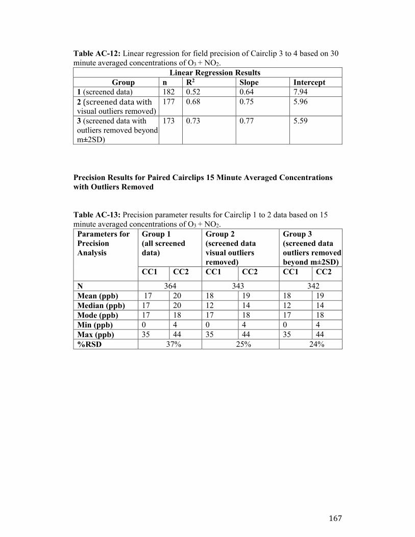
167
Table AC-12: Linear regression for field precision of Cairclip 3 to 4 based on 30
minute averaged concentrations of O3 + NO2.
Linear Regression Results
Group n R2 Slope Intercept
1 (screened data) 182 0.52 0.64 7.94
2 (screened data with visual outliers removed)
177 0.68 0.75 5.96
3 (screened data with
outliers removed beyond
m±2SD)
173 0.73 0.77 5.59
Precision Results for Paired Cairclips 15 Minute Averaged Concentrations
with Outliers Removed
Table AC-13: Precision parameter results for Cairclip 1 to 2 data based on 15
minute averaged concentrations of O3 + NO2.
Parameters for
Precision
Analysis
Group 1
(all screened
data)
Group 2
(screened data
visual outliers
removed)
Group 3
(screened data
outliers removed
beyond m±2SD)
CC1 CC2 CC1 CC2 CC1 CC2
N 364 343 342
Mean (ppb) 17 20 18 19 18 19
Median (ppb) 17 20 12 14 12 14
Mode (ppb) 17 18 17 18 17 18
Min (ppb) 0 4 0 4 0 4
Max (ppb) 35 44 35 44 35 44
%RSD 37% 25% 24%
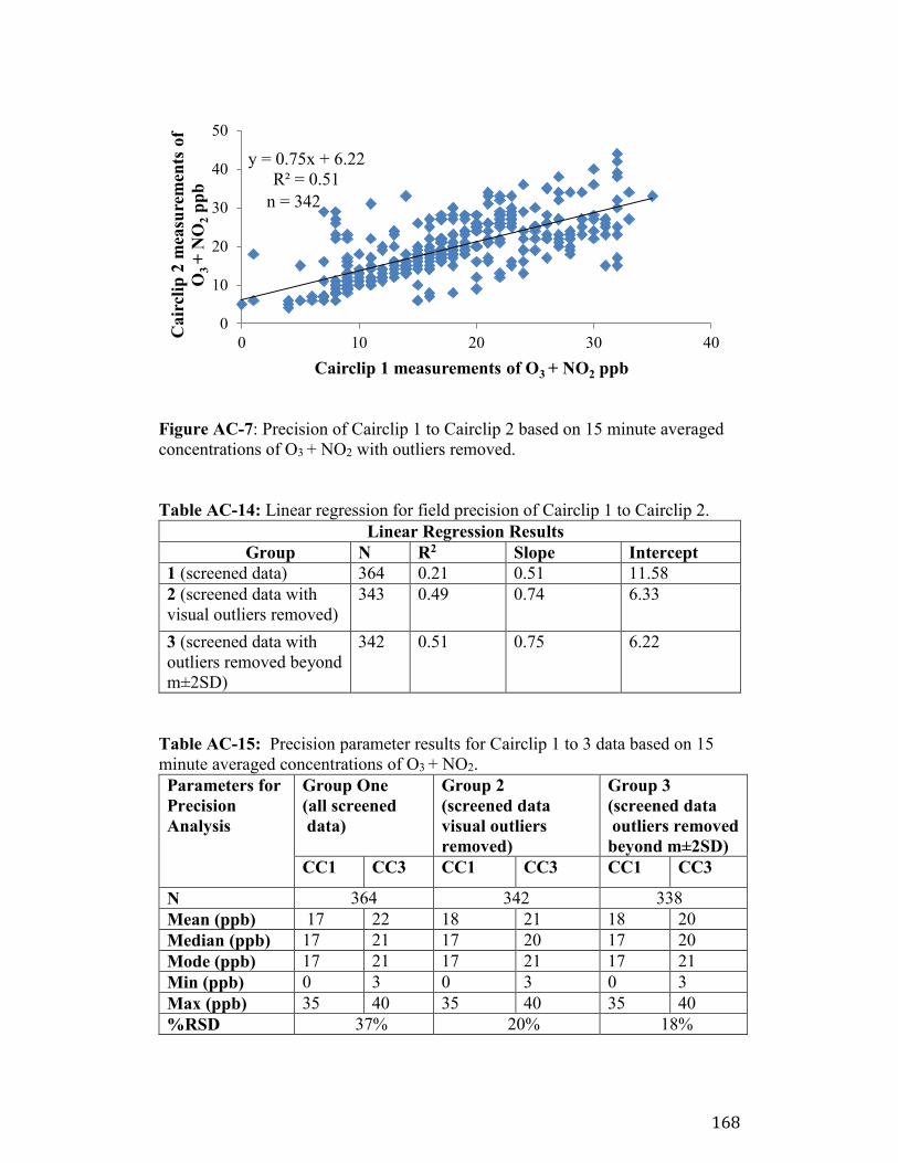
168
Figure AC-7: Precision of Cairclip 1 to Cairclip 2 based on 15 minute averaged
concentrations of O3 + NO2 with outliers removed.
Table AC-14: Linear regression for field precision of Cairclip 1 to Cairclip 2.
Linear Regression Results
Group N R2 Slope Intercept
1 (screened data) 364 0.21 0.51 11.58
2 (screened data with
visual outliers removed)
343 0.49 0.74 6.33
3 (screened data with
outliers removed beyond
m±2SD)
342 0.51 0.75 6.22
Table AC-15: Precision parameter results for Cairclip 1 to 3 data based on 15
minute averaged concentrations of O3 + NO2.
Parameters for
Precision
Analysis
Group One
(all screened
data)
Group 2
(screened data
visual outliers
removed)
Group 3
(screened data
outliers removed
beyond m±2SD)
CC1 CC3 CC1 CC3 CC1 CC3
N 364 342 338
Mean (ppb) 17 22 18 21 18 20
Median (ppb) 17 21 17 20 17 20
Mode (ppb) 17 21 17 21 17 21
Min (ppb) 0 3 0 3 0 3
Max (ppb) 35 40 35 40 35 40
%RSD 37% 20% 18%
y = 0.75x + 6.22
R² = 0.51
0
10
20
30
40
50
0 10 20 30 40
Cair
clip
2 m
easu
rem
ents
of
O3
+ N
O2
pp
b
Cairclip 1 measurements of O3 + NO2 ppb
n = 342
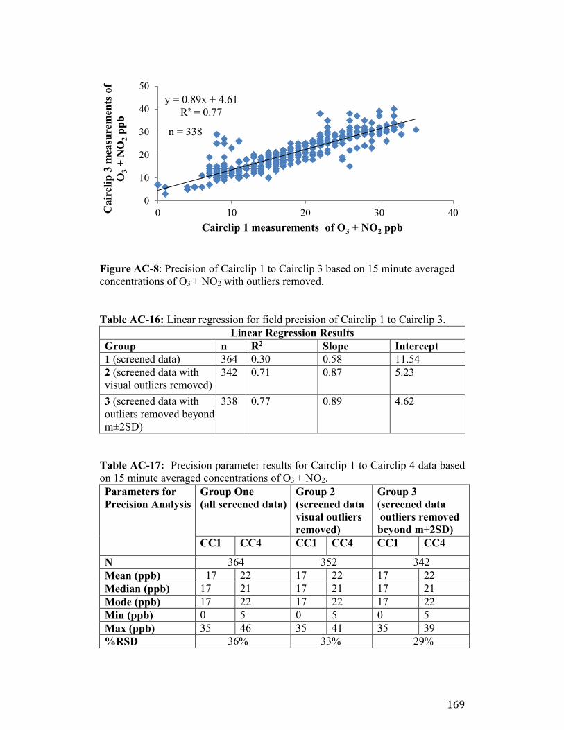
169
Figure AC-8: Precision of Cairclip 1 to Cairclip 3 based on 15 minute averaged
concentrations of O3 + NO2 with outliers removed.
Table AC-16: Linear regression for field precision of Cairclip 1 to Cairclip 3.
Linear Regression Results
Group n R2 Slope Intercept
1 (screened data) 364 0.30 0.58 11.54
2 (screened data with
visual outliers removed)
342 0.71 0.87 5.23
3 (screened data with
outliers removed beyond
m±2SD)
338 0.77 0.89 4.62
Table AC-17: Precision parameter results for Cairclip 1 to Cairclip 4 data based
on 15 minute averaged concentrations of O3 + NO2.
Parameters for
Precision Analysis
Group One
(all screened data)
Group 2
(screened data
visual outliers
removed)
Group 3
(screened data
outliers removed
beyond m±2SD)
CC1 CC4 CC1 CC4 CC1 CC4
N 364 352 342
Mean (ppb) 17 22 17 22 17 22
Median (ppb) 17 21 17 21 17 21
Mode (ppb) 17 22 17 22 17 22
Min (ppb) 0 5 0 5 0 5
Max (ppb) 35 46 35 41 35 39
%RSD 36% 33% 29%
y = 0.89x + 4.61
R² = 0.77
0
10
20
30
40
50
0 10 20 30 40Ca
ircl
ip 3
mea
sure
men
ts o
f
O3
+ N
O2
pp
b
Cairclip 1 measurements of O3 + NO2 ppb
n = 338
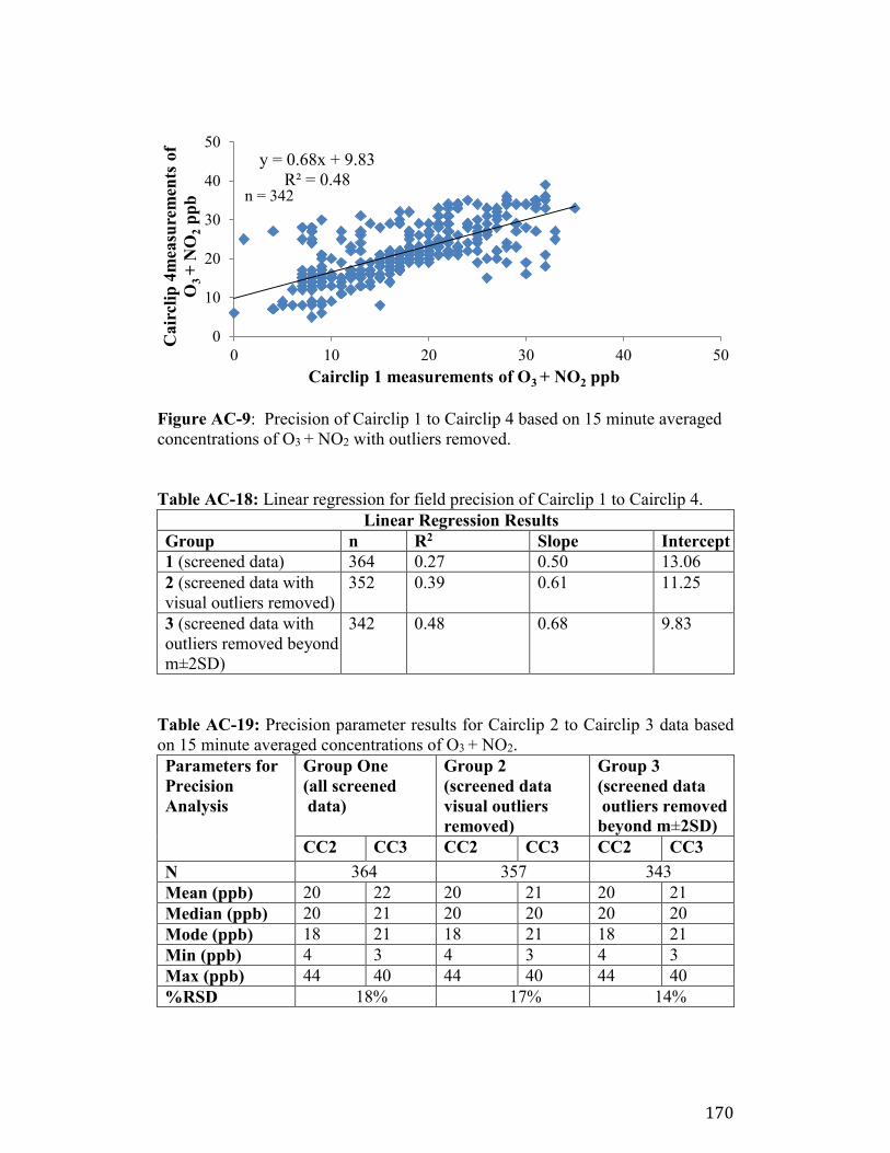
170
Figure AC-9: Precision of Cairclip 1 to Cairclip 4 based on 15 minute averaged
concentrations of O3 + NO2 with outliers removed.
Table AC-18: Linear regression for field precision of Cairclip 1 to Cairclip 4.
Linear Regression Results
Group n R2 Slope Intercept
1 (screened data) 364 0.27 0.50 13.06
2 (screened data with
visual outliers removed)
352 0.39 0.61 11.25
3 (screened data with
outliers removed beyond
m±2SD)
342 0.48 0.68 9.83
Table AC-19: Precision parameter results for Cairclip 2 to Cairclip 3 data based
on 15 minute averaged concentrations of O3 + NO2.
Parameters for
Precision
Analysis
Group One
(all screened
data)
Group 2
(screened data
visual outliers
removed)
Group 3
(screened data
outliers removed
beyond m±2SD)
CC2 CC3 CC2 CC3 CC2 CC3
N 364 357 343
Mean (ppb) 20 22 20 21 20 21
Median (ppb) 20 21 20 20 20 20
Mode (ppb) 18 21 18 21 18 21
Min (ppb) 4 3 4 3 4 3
Max (ppb) 44 40 44 40 44 40
%RSD 18% 17% 14%
y = 0.68x + 9.83
R² = 0.48
0
10
20
30
40
50
0 10 20 30 40 50
Ca
ircl
ip 4
mea
sure
men
ts o
f
O3
+ N
O2
pp
b
Cairclip 1 measurements of O3 + NO2 ppb
n = 342
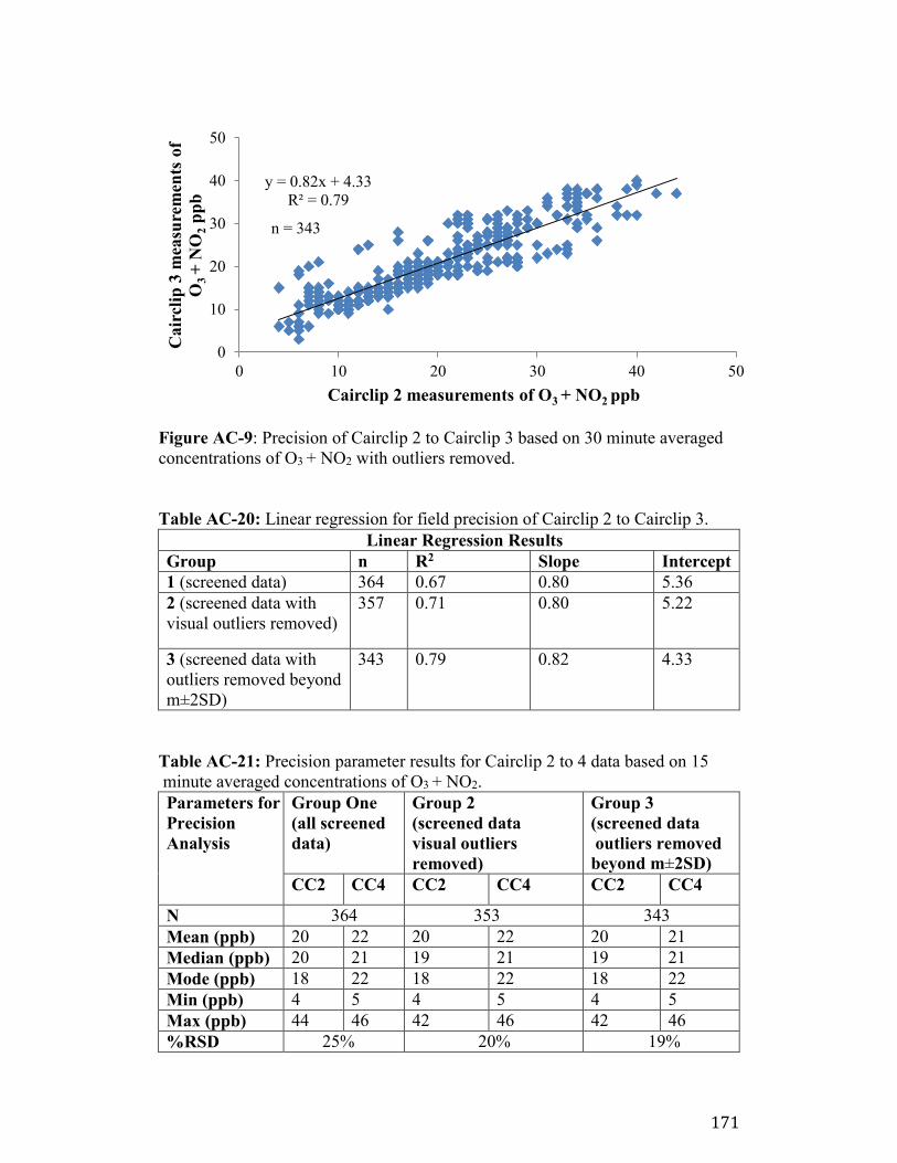
171
Figure AC-9: Precision of Cairclip 2 to Cairclip 3 based on 30 minute averaged
concentrations of O3 + NO2 with outliers removed.
Table AC-20: Linear regression for field precision of Cairclip 2 to Cairclip 3.
Linear Regression Results
Group n R2 Slope Intercept
1 (screened data) 364 0.67 0.80 5.36
2 (screened data with
visual outliers removed)
357 0.71 0.80 5.22
3 (screened data with
outliers removed beyond
m±2SD)
343 0.79 0.82 4.33
Table AC-21: Precision parameter results for Cairclip 2 to 4 data based on 15
minute averaged concentrations of O3 + NO2.
Parameters for
Precision
Analysis
Group One
(all screened
data)
Group 2
(screened data
visual outliers
removed)
Group 3
(screened data
outliers removed
beyond m±2SD)
CC2 CC4 CC2 CC4 CC2 CC4
N 364 353 343
Mean (ppb) 20 22 20 22 20 21
Median (ppb) 20 21 19 21 19 21
Mode (ppb) 18 22 18 22 18 22
Min (ppb) 4 5 4 5 4 5
Max (ppb) 44 46 42 46 42 46
%RSD 25% 20% 19%
y = 0.82x + 4.33
R² = 0.79
0
10
20
30
40
50
0 10 20 30 40 50
Cair
clip
3 m
easu
rem
ents
of
O3
+ N
O2
pp
b
Cairclip 2 measurements of O3 + NO2 ppb
n = 343
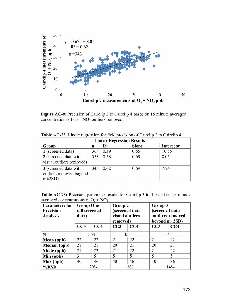
172
Figure AC-9: Precision of Cairclip 2 to Cairclip 4 based on 15 minute averaged
concentrations of O3 + NO2 outliers removed.
Table AC-22: Linear regression for field precision of Cairclip 2 to Cairclip 4.
Linear Regression Results
Group n R2 Slope Intercept
1 (screened data) 364 0.39 0.55 10.55
2 (screened data with
visual outliers removed)
353 0.58 0.69 8.05
3 (screened data with
outliers removed beyond
m±2SD)
343 0.62 0.69 7.74
Table AC-23: Precision parameter results for Cairclip 3 to 4 based on 15 minute
averaged concentrations of O3 + NO2.
Parameters for
Precision
Analysis
Group One
(all screened
data)
Group 2
(screened data
visual outliers
removed)
Group 3
(screened data
outliers removed
beyond m±2SD)
CC3 CC4 CC3 CC4 CC3 CC4
N 364 353 341
Mean (ppb) 22 22 21 22 21 22
Median (ppb) 21 21 20 21 20 21
Mode (ppb) 21 22 21 22 21 22
Min (ppb) 3 5 5 5 5 5
Max (ppb) 40 46 40 46 40 36
%RSD 20% 16% 14%
y = 0.67x + 8.01
R² = 0.62
0
10
20
30
40
50
0 10 20 30 40 50
Ca
ircl
ip 4
mea
sure
men
ts o
f
O3
+ N
O2
pp
b
Cairclip 2 measurements of O3 + NO2 ppb
n =343
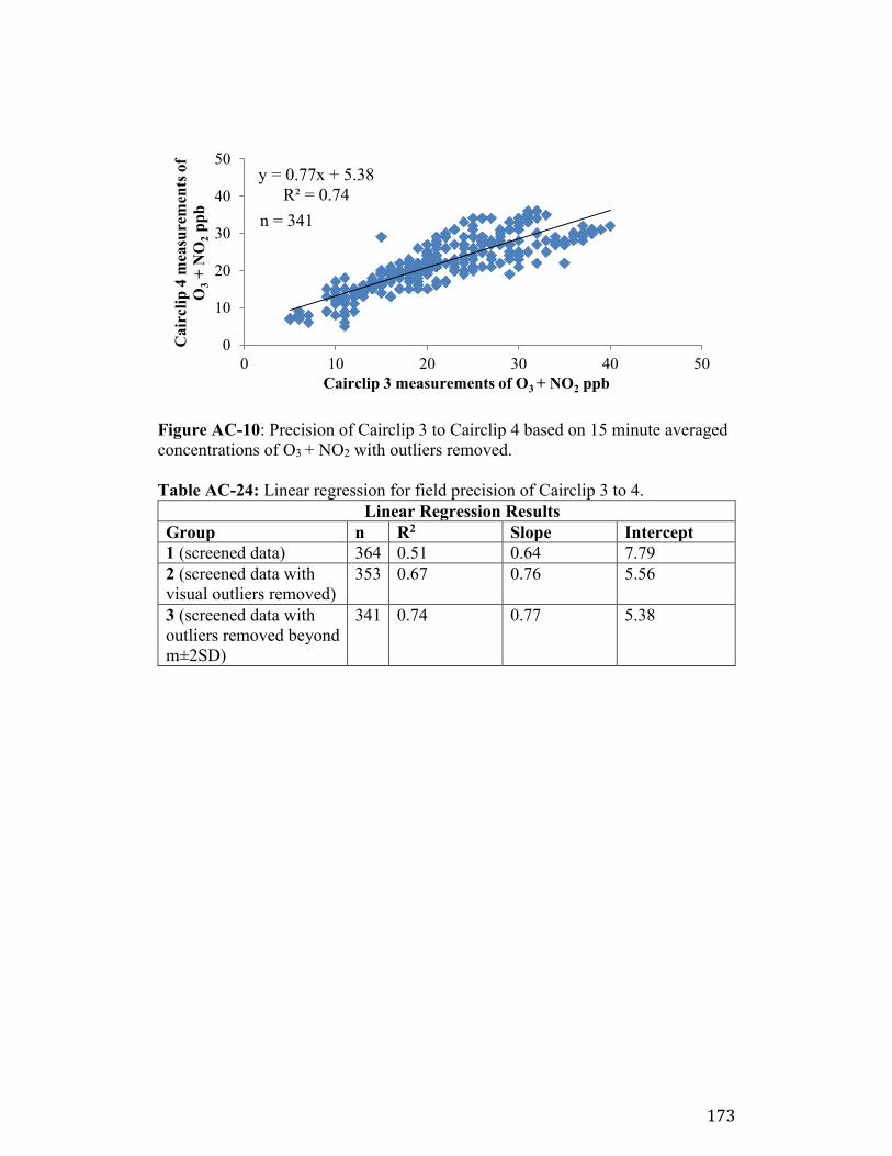
173
Figure AC-10: Precision of Cairclip 3 to Cairclip 4 based on 15 minute averaged
concentrations of O3 + NO2 with outliers removed.
Table AC-24: Linear regression for field precision of Cairclip 3 to 4.
Linear Regression Results
Group n R2 Slope Intercept
1 (screened data) 364 0.51 0.64 7.79
2 (screened data with
visual outliers removed)
353 0.67 0.76 5.56
3 (screened data with
outliers removed beyond
m±2SD)
341 0.74 0.77 5.38
y = 0.77x + 5.38
R² = 0.74
0
10
20
30
40
50
0 10 20 30 40 50
Ca
ircl
ip 4
mea
sure
men
ts o
f
O3
+ N
O2
pp
b
Cairclip 3 measurements of O3 + NO2 ppb
n = 341
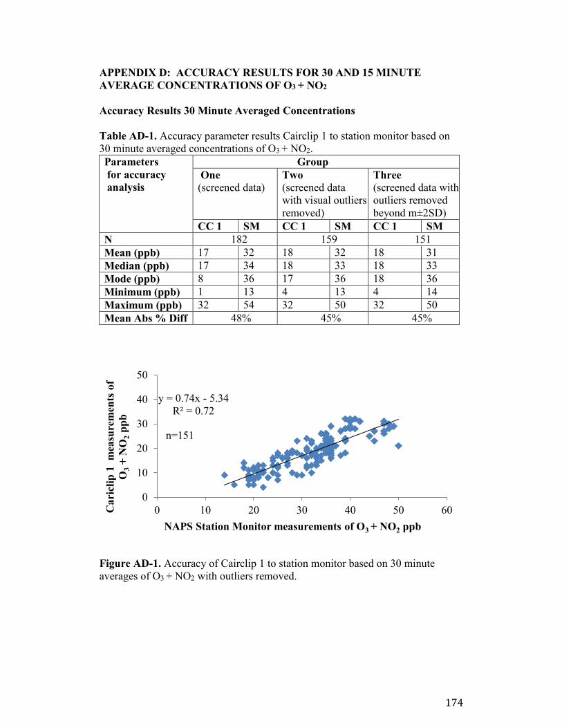
174
APPENDIX D: ACCURACY RESULTS FOR 30 AND 15 MINUTE
AVERAGE CONCENTRATIONS OF O3 + NO2
Accuracy Results 30 Minute Averaged Concentrations
Table AD-1. Accuracy parameter results Cairclip 1 to station monitor based on
30 minute averaged concentrations of O3 + NO2.
Parameters
for accuracy
analysis
Group
One
(screened data)
Two
(screened data
with visual outliers
removed)
Three
(screened data with
outliers removed
beyond m±2SD)
CC 1 SM CC 1 SM CC 1 SM
N 182 159 151
Mean (ppb) 17 32 18 32 18 31
Median (ppb) 17 34 18 33 18 33
Mode (ppb) 8 36 17 36 18 36
Minimum (ppb) 1 13 4 13 4 14
Maximum (ppb) 32 54 32 50 32 50
Mean Abs % Diff 48% 45% 45%
Figure AD-1. Accuracy of Cairclip 1 to station monitor based on 30 minute
averages of O3 + NO2 with outliers removed.
y = 0.74x - 5.34
R² = 0.72
0
10
20
30
40
50
0 10 20 30 40 50 60Cari
clip
1
mea
sure
men
ts o
f
O3
+ N
O2
pp
b
NAPS Station Monitor measurements of O3 + NO2 ppb
n=151
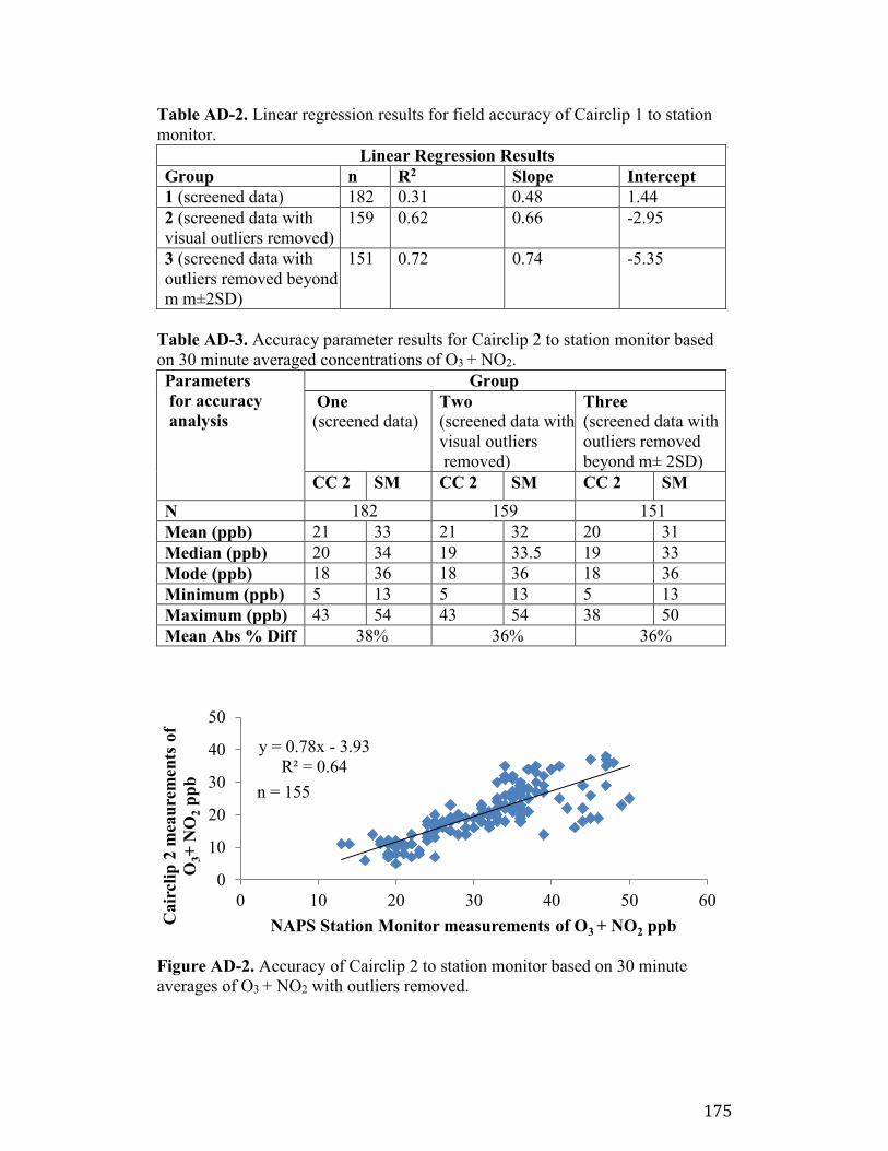
175
Table AD-2. Linear regression results for field accuracy of Cairclip 1 to station
monitor.
Linear Regression Results
Group n R2 Slope Intercept
1 (screened data) 182 0.31 0.48 1.44
2 (screened data with
visual outliers removed)
159 0.62 0.66 -2.95
3 (screened data with
outliers removed beyond
m m±2SD)
151 0.72 0.74 -5.35
Table AD-3. Accuracy parameter results for Cairclip 2 to station monitor based
on 30 minute averaged concentrations of O3 + NO2.
Parameters
for accuracy
analysis
Group
One
(screened data)
Two
(screened data with
visual outliers
removed)
Three
(screened data with
outliers removed
beyond m± 2SD)
CC 2 SM CC 2 SM CC 2 SM
N 182 159 151
Mean (ppb) 21 33 21 32 20 31
Median (ppb) 20 34 19 33.5 19 33
Mode (ppb) 18 36 18 36 18 36
Minimum (ppb) 5 13 5 13 5 13
Maximum (ppb) 43 54 43 54 38 50
Mean Abs % Diff 38% 36% 36%
Figure AD-2. Accuracy of Cairclip 2 to station monitor based on 30 minute
averages of O3 + NO2 with outliers removed.
y = 0.78x - 3.93
R² = 0.64
0
10
20
30
40
50
0 10 20 30 40 50 60
Cair
clip
2 m
eau
rem
ents
of
O3+
NO
2p
pb
NAPS Station Monitor measurements of O3 + NO2 ppb
n = 155
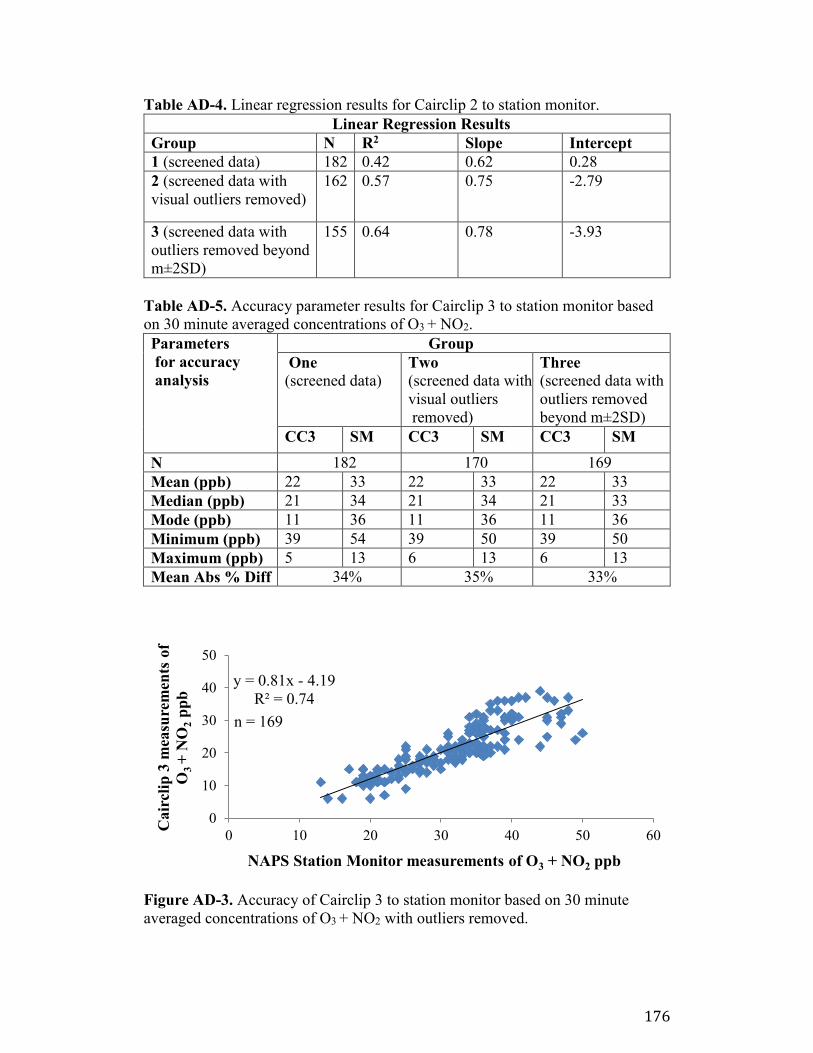
176
Table AD-4. Linear regression results for Cairclip 2 to station monitor.
Linear Regression Results
Group N R2 Slope Intercept
1 (screened data) 182 0.42 0.62 0.28
2 (screened data with
visual outliers removed)
162 0.57 0.75 -2.79
3 (screened data with
outliers removed beyond
m±2SD)
155 0.64 0.78 -3.93
Table AD-5. Accuracy parameter results for Cairclip 3 to station monitor based
on 30 minute averaged concentrations of O3 + NO2.
Parameters
for accuracy
analysis
Group
One
(screened data)
Two
(screened data with
visual outliers
removed)
Three
(screened data with
outliers removed
beyond m±2SD)
CC3 SM CC3 SM CC3 SM
N 182 170 169
Mean (ppb) 22 33 22 33 22 33
Median (ppb) 21 34 21 34 21 33
Mode (ppb) 11 36 11 36 11 36
Minimum (ppb) 39 54 39 50 39 50
Maximum (ppb) 5 13 6 13 6 13
Mean Abs % Diff 34% 35% 33%
Figure AD-3. Accuracy of Cairclip 3 to station monitor based on 30 minute
averaged concentrations of O3 + NO2 with outliers removed.
y = 0.81x - 4.19
R² = 0.74
0
10
20
30
40
50
0 10 20 30 40 50 60
Cair
clip
3 m
easu
rem
ents
of
O3
+ N
O2
pp
b
NAPS Station Monitor measurements of O3 + NO2 ppb
n = 169
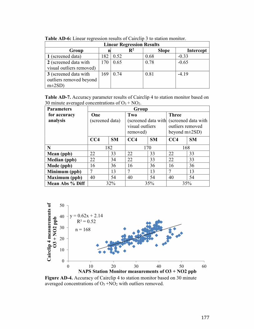
177
Table AD-6: Linear regression results of Cairclip 3 to station monitor.
Linear Regression Results
Group n R2 Slope Intercept
1 (screened data) 182 0.52 0.68 -0.33
2 (screened data with
visual outliers removed)
170 0.65 0.78 -0.65
3 (screened data with
outliers removed beyond
m±2SD)
169 0.74 0.81 -4.19
Table AD-7. Accuracy parameter results of Cairclip 4 to station monitor based on
30 minute averaged concentrations of O3 + NO2.
Parameters
for accuracy
analysis
Group
One
(screened data)
Two
(screened data with
visual outliers
removed)
Three
(screened data with
outliers removed
beyond m±2SD)
CC4 SM CC4 SM CC4 SM
N 182 170 168
Mean (ppb) 22 33 22 33 22 33
Median (ppb) 22 34 22 33 22 33
Mode (ppb) 16 36 16 36 16 36
Minimum (ppb) 7 13 7 13 7 13
Maximum (ppb) 40 54 40 54 40 54
Mean Abs % Diff 32% 35% 35%
Figure AD-4. Accuracy of Cairclip 4 to station monitor based on 30 minute
averaged concentrations of O3 +NO2 with outliers removed.
y = 0.62x + 2.14
R² = 0.52
0
10
20
30
40
50
0 10 20 30 40 50 60
Cair
clip
4 m
easu
rem
ents
of
O3 +
NO
2 p
pb
NAPS Station Monitor measurements of O3 + NO2 ppb
n = 168
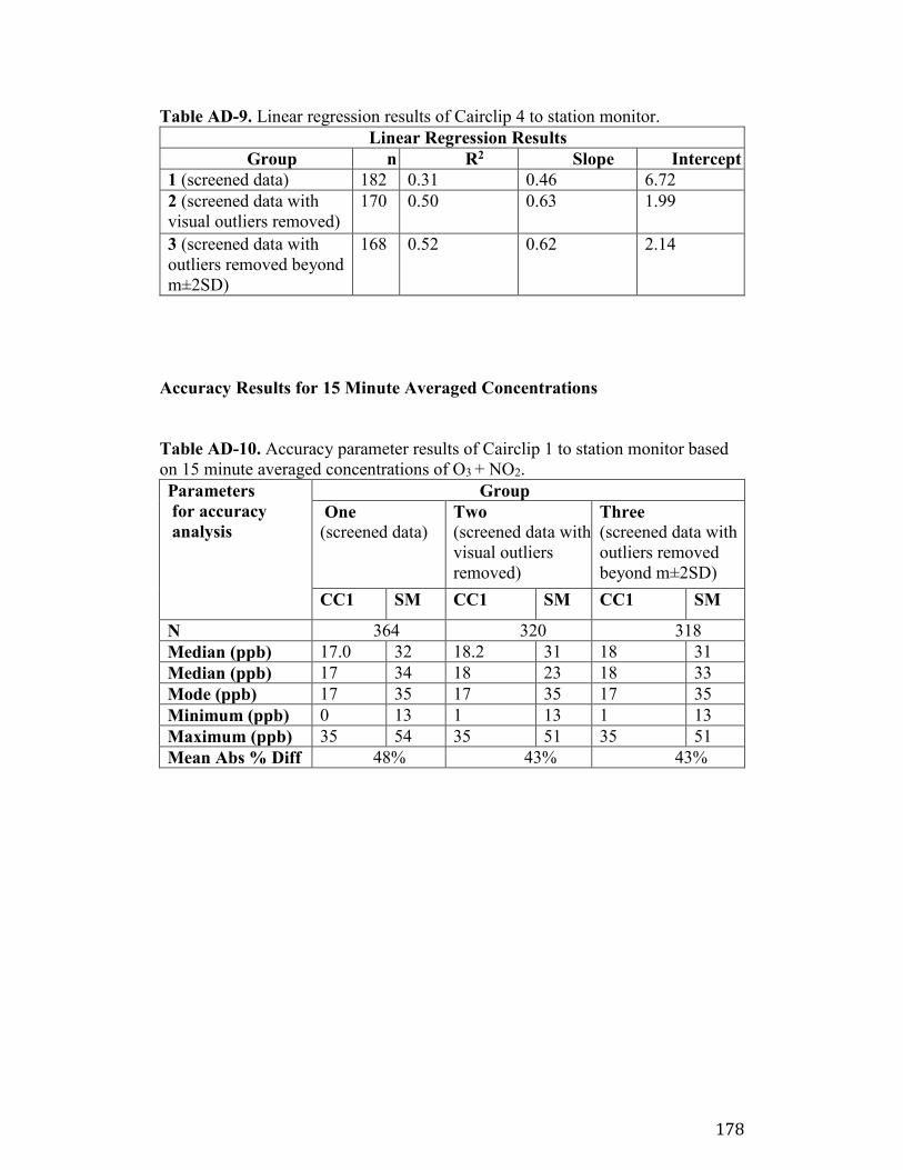
178
Table AD-9. Linear regression results of Cairclip 4 to station monitor.
Linear Regression Results
Group n R2 Slope Intercept
1 (screened data) 182 0.31 0.46 6.72
2 (screened data with
visual outliers removed)
170 0.50 0.63 1.99
3 (screened data with
outliers removed beyond
m±2SD)
168 0.52 0.62 2.14
Accuracy Results for 15 Minute Averaged Concentrations
Table AD-10. Accuracy parameter results of Cairclip 1 to station monitor based
on 15 minute averaged concentrations of O3 + NO2.
Parameters
for accuracy
analysis
Group
One
(screened data)
Two
(screened data with
visual outliers
removed)
Three
(screened data with
outliers removed
beyond m±2SD)
CC1 SM CC1 SM CC1 SM
N 364 320 318
Median (ppb) 17.0 32 18.2 31 18 31
Median (ppb) 17 34 18 23 18 33
Mode (ppb) 17 35 17 35 17 35
Minimum (ppb) 0 13 1 13 1 13
Maximum (ppb) 35 54 35 51 35 51
Mean Abs % Diff 48% 43% 43%
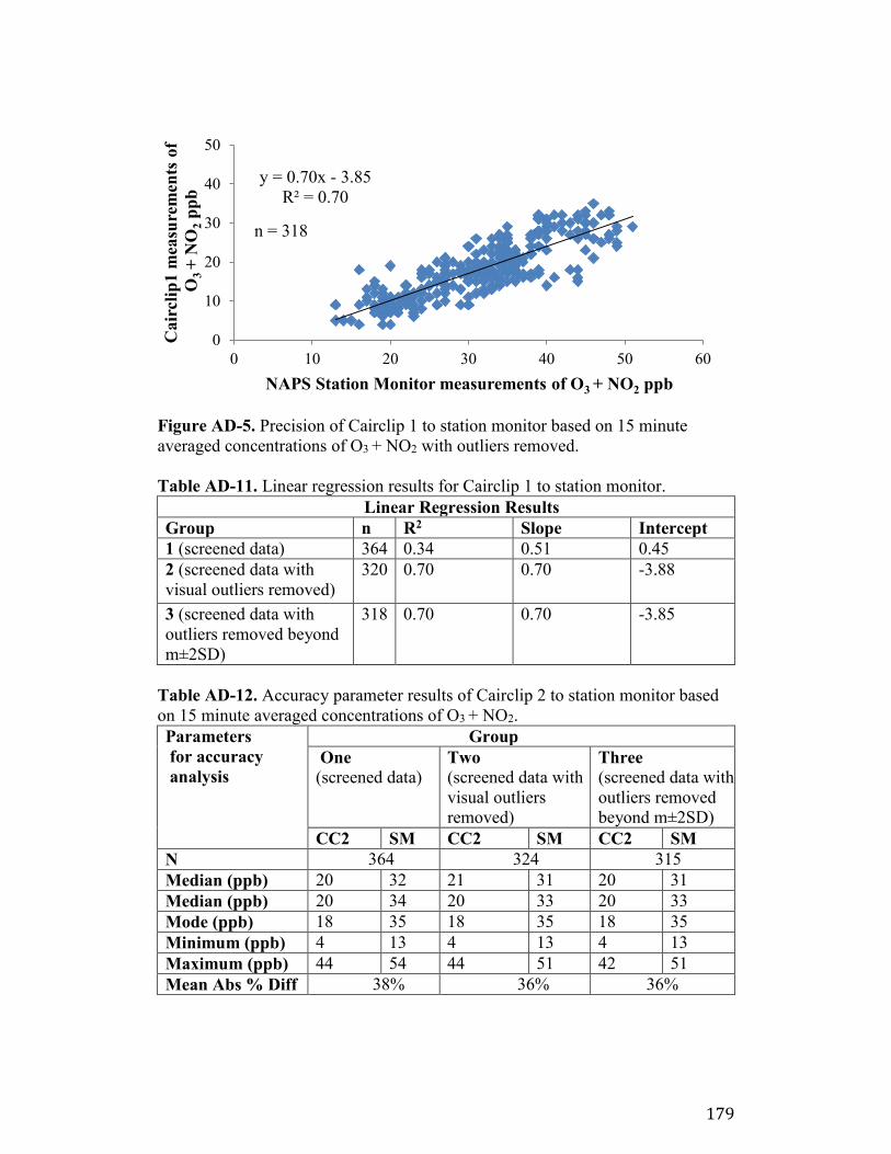
179
Figure AD-5. Precision of Cairclip 1 to station monitor based on 15 minute
averaged concentrations of O3 + NO2 with outliers removed.
Table AD-11. Linear regression results for Cairclip 1 to station monitor.
Linear Regression Results
Group n R2 Slope Intercept
1 (screened data) 364 0.34 0.51 0.45
2 (screened data with
visual outliers removed)
320 0.70 0.70 -3.88
3 (screened data with
outliers removed beyond
m±2SD)
318 0.70 0.70 -3.85
Table AD-12. Accuracy parameter results of Cairclip 2 to station monitor based
on 15 minute averaged concentrations of O3 + NO2.
Parameters
for accuracy
analysis
Group
One
(screened data)
Two
(screened data with
visual outliers
removed)
Three
(screened data with
outliers removed
beyond m±2SD)
CC2 SM CC2 SM CC2 SM
N 364 324 315
Median (ppb) 20 32 21 31 20 31
Median (ppb) 20 34 20 33 20 33
Mode (ppb) 18 35 18 35 18 35
Minimum (ppb) 4 13 4 13 4 13
Maximum (ppb) 44 54 44 51 42 51
Mean Abs % Diff 38% 36% 36%
y = 0.70x - 3.85
R² = 0.70
0
10
20
30
40
50
0 10 20 30 40 50 60
Cair
clip
1 m
easu
rem
ents
of
O3
+ N
O2
pp
b
NAPS Station Monitor measurements of O3 + NO2 ppb
n = 318
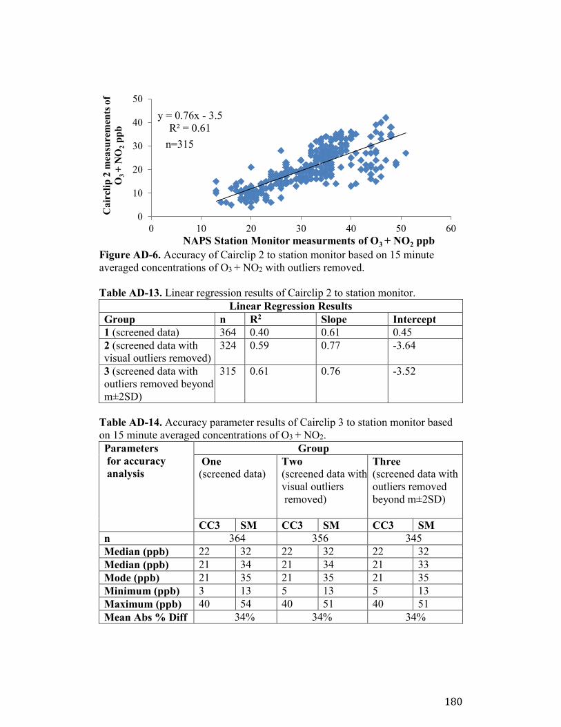
180
Figure AD-6. Accuracy of Cairclip 2 to station monitor based on 15 minute
averaged concentrations of O3 + NO2 with outliers removed.
Table AD-13. Linear regression results of Cairclip 2 to station monitor.
Linear Regression Results
Group n R2 Slope Intercept
1 (screened data) 364 0.40 0.61 0.45
2 (screened data with
visual outliers removed)
324 0.59 0.77 -3.64
3 (screened data with
outliers removed beyond
m±2SD)
315 0.61 0.76 -3.52
Table AD-14. Accuracy parameter results of Cairclip 3 to station monitor based
on 15 minute averaged concentrations of O3 + NO2.
Parameters
for accuracy
analysis
Group
One
(screened data)
Two
(screened data with
visual outliers
removed)
Three
(screened data with
outliers removed
beyond m±2SD)
CC3 SM CC3 SM CC3 SM
n 364 356 345
Median (ppb) 22 32 22 32 22 32
Median (ppb) 21 34 21 34 21 33
Mode (ppb) 21 35 21 35 21 35
Minimum (ppb) 3 13 5 13 5 13
Maximum (ppb) 40 54 40 51 40 51
Mean Abs % Diff 34% 34% 34%
y = 0.76x - 3.5
R² = 0.61
0
10
20
30
40
50
0 10 20 30 40 50 60
Cair
clip
2 m
easu
rem
ents
of
O3
+ N
O2
pp
b
NAPS Station Monitor measurments of O3 + NO2 ppb
n=315
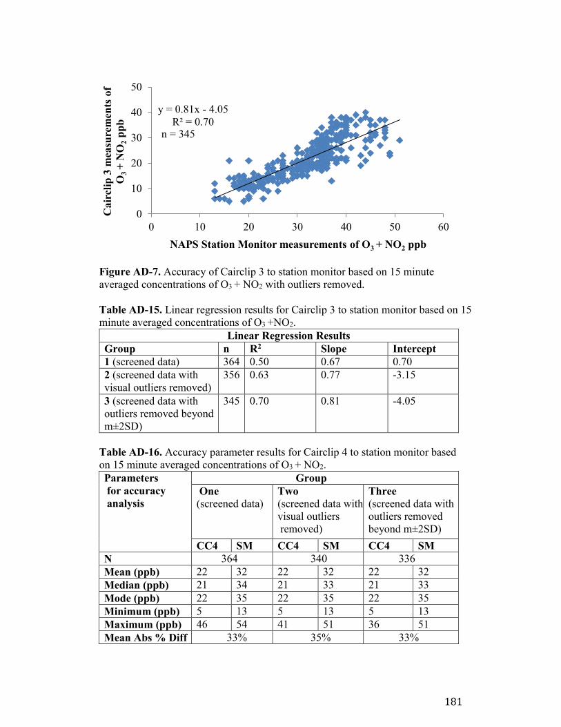
181
Figure AD-7. Accuracy of Cairclip 3 to station monitor based on 15 minute
averaged concentrations of O3 + NO2 with outliers removed.
Table AD-15. Linear regression results for Cairclip 3 to station monitor based on 15
minute averaged concentrations of O3 +NO2.
Linear Regression Results
Group n R2 Slope Intercept
1 (screened data) 364 0.50 0.67 0.70
2 (screened data with
visual outliers removed)
356 0.63 0.77 -3.15
3 (screened data with
outliers removed beyond
m±2SD)
345 0.70 0.81 -4.05
Table AD-16. Accuracy parameter results for Cairclip 4 to station monitor based
on 15 minute averaged concentrations of O3 + NO2.
Parameters
for accuracy
analysis
Group
One
(screened data)
Two
(screened data with
visual outliers
removed)
Three
(screened data with
outliers removed
beyond m±2SD)
CC4 SM CC4 SM CC4 SM
N 364 340 336
Mean (ppb) 22 32 22 32 22 32
Median (ppb) 21 34 21 33 21 33
Mode (ppb) 22 35 22 35 22 35
Minimum (ppb) 5 13 5 13 5 13
Maximum (ppb) 46 54 41 51 36 51
Mean Abs % Diff 33% 35% 33%
y = 0.81x - 4.05
R² = 0.70
0
10
20
30
40
50
0 10 20 30 40 50 60
Cair
clip
3 m
easu
rem
ents
of
O3
+ N
O2
pp
b
NAPS Station Monitor measurements of O3 + NO2 ppb
n = 345
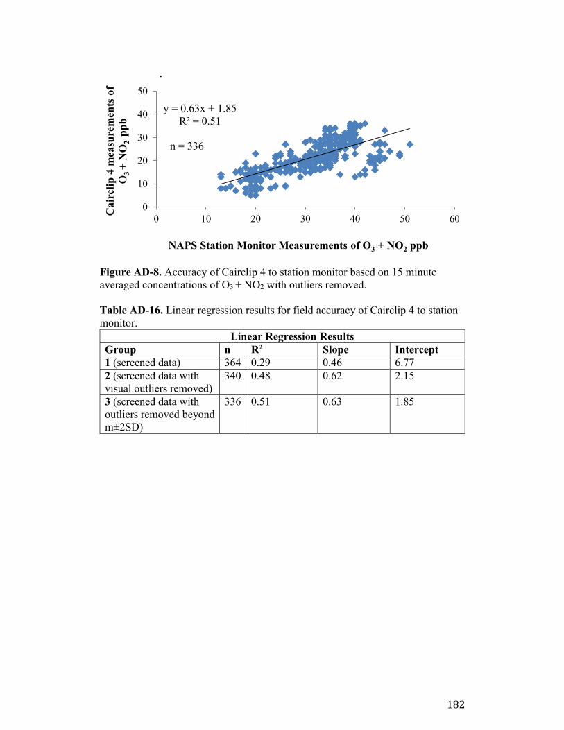
182
Figure AD-8. Accuracy of Cairclip 4 to station monitor based on 15 minute
averaged concentrations of O3 + NO2 with outliers removed.
Table AD-16. Linear regression results for field accuracy of Cairclip 4 to station
monitor.
Linear Regression Results
Group n R2 Slope Intercept
1 (screened data) 364 0.29 0.46 6.77
2 (screened data with
visual outliers removed)
340 0.48 0.62 2.15
3 (screened data with
outliers removed beyond
m±2SD)
336 0.51 0.63 1.85
y = 0.63x + 1.85
R² = 0.51
0
10
20
30
40
50
0 10 20 30 40 50 60
Cair
clip
4 m
easu
rem
ents
of
O3
+ N
O2
p
pb
NAPS Station Monitor Measurements of O3 + NO2 ppb
.
n = 336
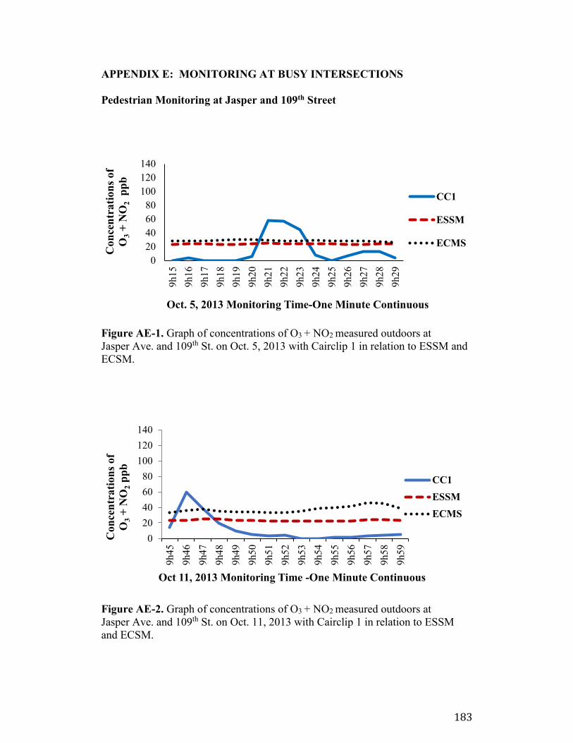
183
APPENDIX E: MONITORING AT BUSY INTERSECTIONS
Pedestrian Monitoring at Jasper and 109th Street
Figure AE-1. Graph of concentrations of O3 + NO2 measured outdoors at
Jasper Ave. and 109th St. on Oct. 5, 2013 with Cairclip 1 in relation to ESSM and
ECSM.
Figure AE-2. Graph of concentrations of O3 + NO2 measured outdoors at
Jasper Ave. and 109th St. on Oct. 11, 2013 with Cairclip 1 in relation to ESSM
and ECSM.
0
20
40
60
80
100
120
1409h15
9h16
9h17
9h18
9h19
9h20
9h21
9h22
9h23
9h24
9h25
9h26
9h27
9h28
9h29
Con
cen
trati
on
s of
O3
+ N
O2
pp
b
Oct. 5, 2013 Monitoring Time-One Minute Continuous
CC1
ESSM
ECMS
0
20
40
60
80
100
120
140
9h
45
9h
46
9h
47
9h
48
9h
49
9h
50
9h
51
9h
52
9h
53
9h54
9h
55
9h
56
9h
57
9h
58
9h
59
Con
cen
trati
on
s of
O3
+ N
O2
pp
b
Oct 11, 2013 Monitoring Time -One Minute Continuous
CC1
ESSM
ECMS
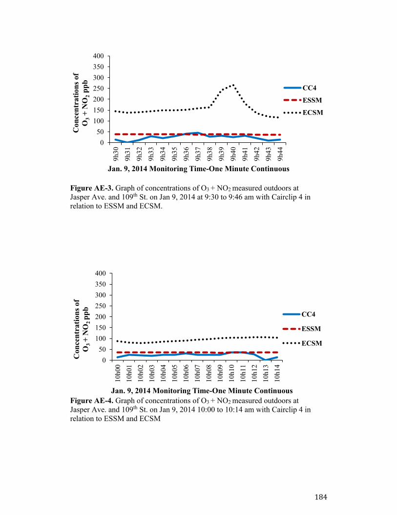
184
Figure AE-3. Graph of concentrations of O3 + NO2 measured outdoors at
Jasper Ave. and 109th St. on Jan 9, 2014 at 9:30 to 9:46 am with Cairclip 4 in
relation to ESSM and ECSM.
Figure AE-4. Graph of concentrations of O3 + NO2 measured outdoors at
Jasper Ave. and 109th St. on Jan 9, 2014 10:00 to 10:14 am with Cairclip 4 in
relation to ESSM and ECSM
0
50
100
150
200
250
300
350
400
9h
30
9h
31
9h
32
9h
33
9h
34
9h
35
9h
36
9h
37
9h
38
9h
39
9h
40
9h
41
9h
42
9h43
9h
44
Co
nce
ntr
ati
on
s o
f
O3
+ N
O2
pp
b
Jan. 9, 2014 Monitoring Time-One Minute Continuous
CC4
ESSM
ECSM
0
50
100
150
200
250
300
350
400
10
h00
10
h01
10
h02
10
h03
10
h04
10
h05
10
h06
10
h07
10
h08
10h09
10
h10
10
h11
10
h12
10
h13
10
h14
Con
cen
trati
on
s of
O3
+ N
O2
pp
b
Jan. 9, 2014 Monitoring Time-One Minute Continuous
CC4
ESSM
ECSM
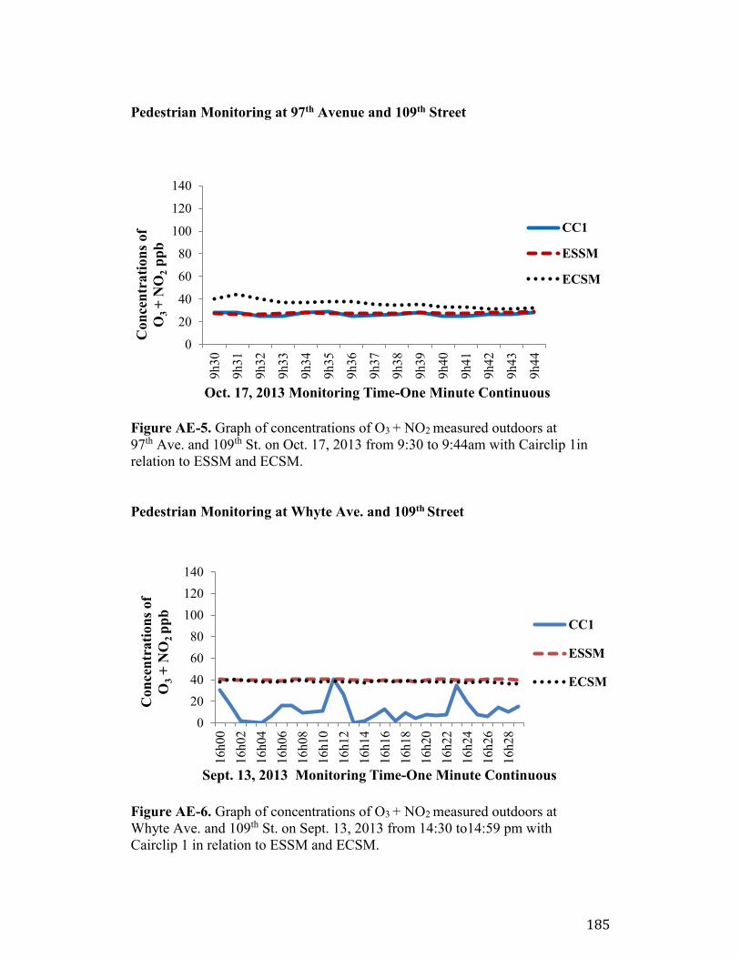
185
Pedestrian Monitoring at 97th Avenue and 109th Street
Figure AE-5. Graph of concentrations of O3 + NO2 measured outdoors at
97th Ave. and 109th St. on Oct. 17, 2013 from 9:30 to 9:44am with Cairclip 1in
relation to ESSM and ECSM.
Pedestrian Monitoring at Whyte Ave. and 109th Street
Figure AE-6. Graph of concentrations of O3 + NO2 measured outdoors at
Whyte Ave. and 109th St. on Sept. 13, 2013 from 14:30 to14:59 pm with
Cairclip 1 in relation to ESSM and ECSM.
0
20
40
60
80
100
120
140
9h30
9h31
9h32
9h33
9h34
9h35
9h36
9h37
9h38
9h39
9h40
9h41
9h42
9h43
9h44
Co
nce
ntr
ati
on
s o
f
O3
+ N
O2
pp
b
Oct. 17, 2013 Monitoring Time-One Minute Continuous
CC1
ESSM
ECSM
0
20
40
60
80
100
120
140
16
h00
16
h02
16
h04
16
h06
16
h08
16
h10
16
h12
16
h14
16
h16
16
h18
16
h20
16
h22
16
h24
16
h26
16
h28
Con
cen
trati
on
s of
O3
+ N
O2
pp
b
Sept. 13, 2013 Monitoring Time-One Minute Continuous
CC1
ESSM
ECSM
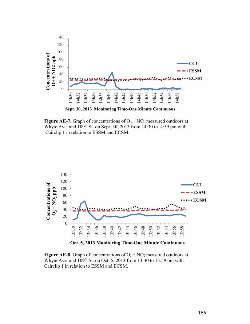
186
Figure AE-7. Graph of concentrations of O3 + NO2 measured outdoors at
Whyte Ave. and 109th St. on Sept. 30, 2013 from 14:30 to14:59 pm with
Cairclip 1 in relation to ESSM and ECSM.
Figure AE-8. Graph of concentrations of O3 + NO2 measured outdoors at
Whyte Ave. and 109th St. on Oct. 5, 2013 from 13:30 to 13:59 pm with
Cairclip 1 in relation to ESSM and ECSM.
020406080100120140
14
h30
14
h32
14
h34
14
h36
14
h38
14
h40
14
h42
14h44
14
h46
14
h48
14
h50
14
h52
14
h54
14
h56
14
h58
Con
cen
trati
on
s of
O3
+ N
O2
pp
b
Sept. 30, 2013 Monitoring Time-One Minute Continuous
CC1
ESSM
ECSM
0
20
40
60
80
100
120
140
13
h30
13
h32
13
h34
13
h36
13
h38
13
h40
13
h42
13
h44
13
h46
13
h48
13
h50
13
h52
13
h54
13
h56
13
h58
Con
cen
trati
on
s of
O3
+ N
O2
pp
b
Oct. 5, 2013 Monitoring Time-One Minute Continuous
CC1
ESSM
ECSM
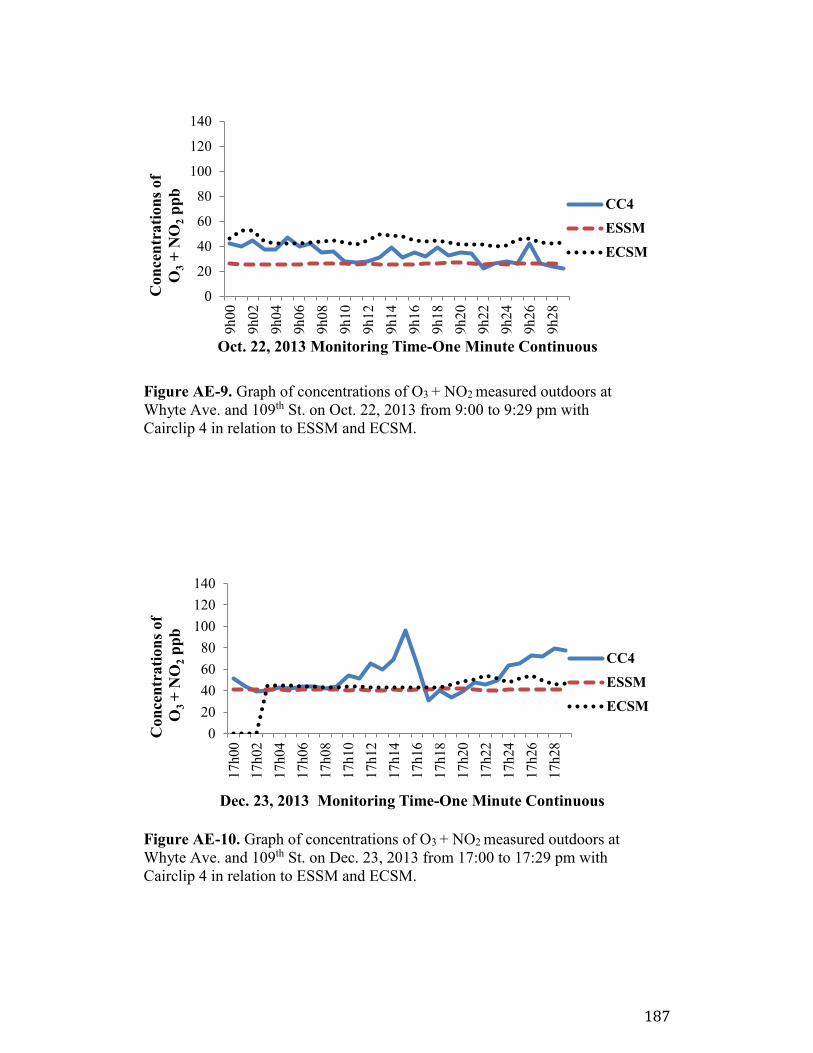
187
Figure AE-9. Graph of concentrations of O3 + NO2 measured outdoors at
Whyte Ave. and 109th St. on Oct. 22, 2013 from 9:00 to 9:29 pm with
Cairclip 4 in relation to ESSM and ECSM.
Figure AE-10. Graph of concentrations of O3 + NO2 measured outdoors at
Whyte Ave. and 109th St. on Dec. 23, 2013 from 17:00 to 17:29 pm with
Cairclip 4 in relation to ESSM and ECSM.
0
20
40
60
80
100
120
140
9h00
9h
02
9h
04
9h
06
9h
08
9h
10
9h
12
9h
14
9h
16
9h
18
9h
20
9h
22
9h
24
9h
26
9h
28
Con
cen
trati
on
s of
O3
+ N
O2
pp
b
Oct. 22, 2013 Monitoring Time-One Minute Continuous
CC4
ESSM
ECSM
0
20
40
60
80
100
120
140
17
h00
17
h02
17
h04
17
h06
17
h08
17
h10
17
h12
17
h14
17
h16
17
h18
17
h20
17
h22
17
h24
17
h26
17h28
Con
cen
trati
on
s of
O3
+ N
O2
pp
b
Dec. 23, 2013 Monitoring Time-One Minute Continuous
CC4
ESSM
ECSM
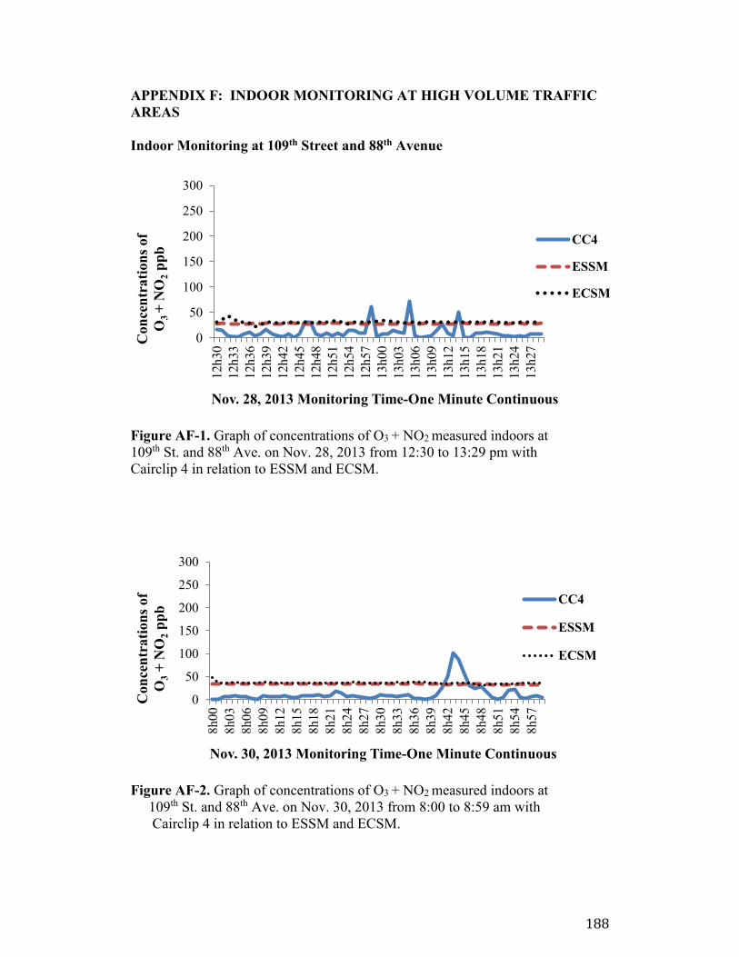
188
APPENDIX F: INDOOR MONITORING AT HIGH VOLUME TRAFFIC
AREAS
Indoor Monitoring at 109th Street and 88th Avenue
Figure AF-1. Graph of concentrations of O3 + NO2 measured indoors at
109th St. and 88th Ave. on Nov. 28, 2013 from 12:30 to 13:29 pm with
Cairclip 4 in relation to ESSM and ECSM.
Figure AF-2. Graph of concentrations of O3 + NO2 measured indoors at
109th St. and 88th Ave. on Nov. 30, 2013 from 8:00 to 8:59 am with
Cairclip 4 in relation to ESSM and ECSM.
0
50
100
150
200
250
300
8h
00
8h
03
8h
06
8h
09
8h12
8h
15
8h
18
8h
21
8h
24
8h
27
8h
30
8h
33
8h
36
8h
39
8h
42
8h
45
8h
48
8h51
8h
54
8h
57
Con
cen
trati
on
s of
O3
+ N
O2
pp
b
Nov. 30, 2013 Monitoring Time-One Minute Continuous
CC4
ESSM
ECSM
0
50
100
150
200
250
300
12h30
12h33
12h36
12h39
12h42
12h45
12h48
12h51
12h54
12h57
13h00
13
h03
13h06
13h09
13h12
13h15
13h18
13h21
13h24
13h27
Con
cen
trati
on
s of
O3
+ N
O2
pp
b
Nov. 28, 2013 Monitoring Time-One Minute Continuous
CC4
ESSM
ECSM
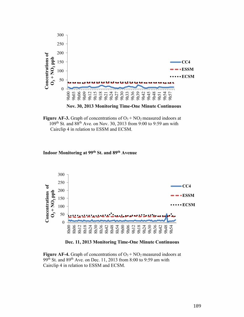
189
Figure AF-3. Graph of concentrations of O3 + NO2 measured indoors at
109th St. and 88th Ave. on Nov. 30, 2013 from 9:00 to 9:59 am with
Cairclip 4 in relation to ESSM and ECSM.
Indoor Monitoring at 99th St. and 89th Avenue
Figure AF-4. Graph of concentrations of O3 + NO2 measured indoors at
99th St. and 89th Ave. on Dec. 11, 2013 from 8:00 to 9:59 am with
Cairclip 4 in relation to ESSM and ECSM.
0
50
100
150
200
250
300
9h
00
9h
03
9h
06
9h
09
9h
12
9h
15
9h
18
9h
21
9h24
9h
27
9h
30
9h33
9h
36
9h
39
9h42
9h
45
9h
48
9h
51
9h
54
9h
57
Co
nce
ntr
ati
on
s o
f
O3
+ N
O2
pp
b
Nov. 30, 2013 Monitoring Time-One Minute Continuous
CC4
ESSM
ECSM
0
50
100
150
200
250
300
8h
00
8h
06
8h
12
8h
18
8h
24
8h
30
8h
36
8h
42
8h
48
8h
54
9h00
9h
06
9h
12
9h
18
9h
24
9h
30
9h
36
9h
42
9h
48
9h
54
Con
cen
trati
on
s o
f
O3
+ N
O2
pp
b
Dec. 11, 2013 Monitoring Time-One Minute Continuous
CC4
ESSM
ECSM
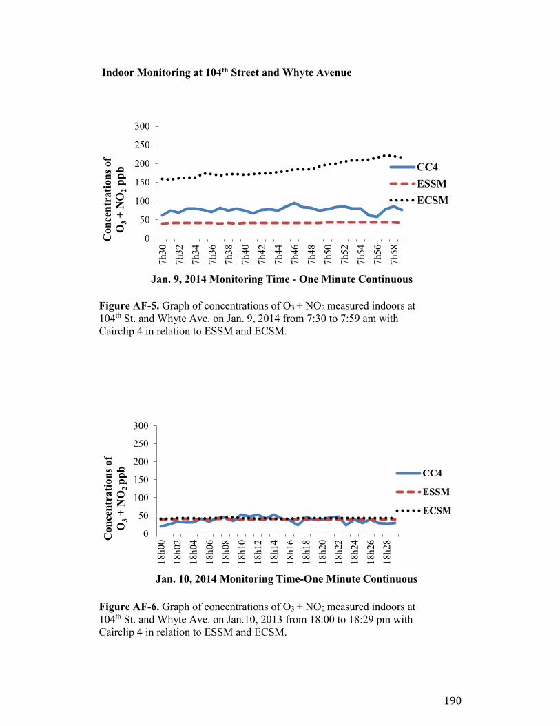
190
Indoor Monitoring at 104th Street and Whyte Avenue
Figure AF-5. Graph of concentrations of O3 + NO2 measured indoors at
104th St. and Whyte Ave. on Jan. 9, 2014 from 7:30 to 7:59 am with
Cairclip 4 in relation to ESSM and ECSM.
Figure AF-6. Graph of concentrations of O3 + NO2 measured indoors at
104th St. and Whyte Ave. on Jan.10, 2013 from 18:00 to 18:29 pm with
Cairclip 4 in relation to ESSM and ECSM.
0
50
100
150
200
250
300
7h
30
7h
32
7h
34
7h
36
7h
38
7h
40
7h
42
7h
44
7h
46
7h
48
7h
50
7h
52
7h
54
7h
56
7h
58
Con
cen
trati
on
s of
O3
+ N
O2
pp
b
Jan. 9, 2014 Monitoring Time - One Minute Continuous
CC4
ESSM
ECSM
0
50
100
150
200
250
300
18
h00
18
h02
18
h04
18
h06
18
h08
18
h10
18
h12
18
h14
18
h16
18
h18
18
h20
18
h22
18
h24
18
h26
18h28C
on
cen
trati
on
s of
O3
+ N
O2
pp
b
Jan. 10, 2014 Monitoring Time-One Minute Continuous
CC4
ESSM
ECSM