A Quarterly Econometric Model of Portfolio Choice — Part II: Portfolio Behaviour of Australian Savings Banks

A Quarterly Econometric Model of Portfolio Choice - Part 11: Portfolio Behaviour of Australian Savings Banks*

In Part I of this study, we derived a portfolio behaviour model based on utility maximization and cost minimization. As a test of the model, i t is now applied t o examine the portfolio behaviour of Australian savings banks.

Institutional Framework It is apparent from a condensed balance sheet of Australian

savings banks, as shown in Table I, that the liabilities of these banks are dominated by depositors’ balances. Such deposits may, with little inconvenience, be converted on demand into cash without capital loss, and yield a nominal return. ‘The terms on which savings banks accept deposits . . . have been fixed after discussion between the Reserve Bank and the banks and with the approval of the Treasurer’ [ 10, p. 161.

We shall therefore assume that the yield on savings deposits is set by the authorities and that the market for these deposits is essentially demand determined. This implies that the banks accept all deposits offered to them by the private sector at the prevailing interest rate, so that the volume of deposits is predetermined as far as the banks are concerned. The liability category, ‘other net liabilities’, is derived as the balancing item SO that total assets equal liabilities. Consequently, we are uncertain as to what is included in the category except that it would contain the capital accounts of the banks. We therefore assume that other net liabilities are predetermined in the model: the savings banks are viewed as decision-makers with respect to the six categories in Table I, given a predetermined level of liabilities.

*The first half of this paper, ‘A Quarterly Econometric Model of Portfolio Choice-Part I : Specification and Estimation Problems’, appeared in Economic Record, Vol. 49, December 1973, pp. 518-33.

31

22 THE ECONOMIC RECORD MARCH

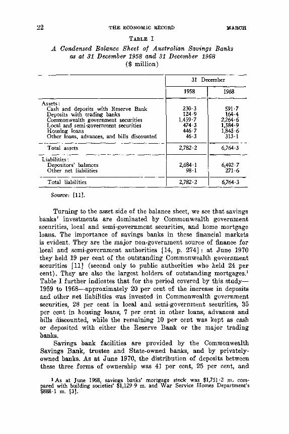
TABLE I A Condensed Balance Sheet of A u s t r a h n Savings Banks

($ million) a.s at 31 December 1958 and 31 December 1968

31 December

Assets : Cash and deposits with Reserve Bank Deposits with trading banks Commonwealth government securities Local and semi-government securities Housing loans Other loans, advances, and bills discounted

230.3 124.9

1.459.7 474.3 446.7 46.3

591.7 164.4

2.264.6 11584.9

I 1,845.6 313.1

Total assets I 2,782.2 1 6,764.3

Liabilities : Depositors’ balances Other net liabilities

2,684.1 98.1

6,492.7 271.6

Total liabilities I 2.782.2 I 6,764.3

Source: [11].

T’urning to the asset side of the balance sheet, we see that savings banks’ investments are dominated by Commonwealth government securities, local and semi-government securities, and home mortgage loans. The importance of savings banks in these financial markets is evident. They are the major non-government source of finance for local and semi-government authorities [14, p. 2741 : a t June 1970 they held 19 per cent of the outstanding Commonwealth government securities [ll] (second only to public authorities who held 24 per cent). They are also the largest holders of outstanding mortgages.’ Table I further indicates that for the period covered by this study- 1959 to 1968-approximately 20 per cent of the increase in deposits and other net liabilities was invested in Commonwealth government securities, 28 per cent in local and semi-government securities, 35 per cent in housing loans, 7 per cent in other loans, advances and bills discounted, while the remaining 10 per cent was kept as cash or deposited with either the Reserve Bank or the major trading banks.

Savings bank facilities are provided by the Commonwealth Saving8 Bank, trustee and State-owned banks, and by privately- owned banks. As at June 1970, the distribution of deposits between these three forms of ownership was 41 per cent, 25 per cent, and

1As at June 1968, savings banks’ mortgage stock was $1,751.2 m, compared with building societies’ $1,129.9 m. and War Service Homes Department’s $888.1 m. [3].

1974 PORTFOLIO CHOICE 23

34 per cent respectively [ll, February 1971, p. 2341. Because the banks are subject to differing legal and social responsibilities i t is not surprising that the disposition of the funds of the private savings banks differs from that of the government-owned and trustee banks. Thus, from 1955 to 1968 the private banks allocated a greater proportion of their increase in deposits to investments in government securities (and a lower percentage to loans, advances, and bills discounted) than the government and trustee banks [3]. Such differences in portfolio behaviour are largely ignored in this study as, with the exception of the 1962-63 fiscal year, the proportion of the increase in total savings deposits attracted to the private banks has not fluctuated greatly over the sample period, although it does show a downward trend.2 It is conceivable then that the regression results may underestimate the change in savings banks’ holdings of Com- monwealth government securities and overestimate the change in home loans for the 1962-63 p e r i ~ d . ~ We shall examine the residuals from the estimating equations to ascertain whether they are compatible with such an hypothesis.

I n addition to interest rate controls, the Reserve Bank requires the savings banks to hold a minimum percentage of depositors’ funds in prescribed assets. This control effectively placed an upper limit on loans to the private sector of 30 per cent prior to August 1963, and 35 per cent from August 1963 to October 1970, when i t was increased once again to 40 per cent. Wallace, writing at the close of 1963, argued that the limits were of no practical significance as ‘the only banks which ever came close to the 30 per cent limit were the two Tasmanian trustee banks, and special arrangements were made for them’ [14, p. 2791. However, owing to the substantial increase in home lending since that time, the proportion of loans to the private sector has increased from 22 per cent a t December 1963 to 28 per cent a t December 1966 and 31.5 per cent a t December 1968.4 It is possible, in the final couple of years of the study and in the ez post forecast period, that this regulatory limit could have restricted the amount lent for home mortgages. This hypothesis is tested by ascertaining whether there is any tendency for the mortgage equation to overestimate the supply of mortgages in these periods.

A second constraint on savings banks’ portfolio behaviour is

2For fiscal years 1958-59 to 1968-69, the proportions were: 0.51, 0.49, 0.51, 0.47, 0.55, 0.48, 0.46, 0.43, 0.45, 0.46,. and 0.45. Calculated from [ l l ] .

3One way of testing the hypothesis that changes in the net deposit flow between private and government and trustee banks influence total asset stock changes would be to include a variable such as the proportion of net deposit changes going to the private banks as an explanatory variable. This approach is not pursued at present because an analysis of the relative competitive position of the various forms of bank ownership is felt to be beyond the scope of this study.

4These are approximations calculated from [ll]. It was assumed that 50 per cent of other loans, advances, and bills discounted were loans to other banks and therefore included in the prescribed assets.

MARCH 24 THE ECONOMIC RECORD

that they must maintain a minimum of 10 per cent of depositors’ funds in deposits with the Reserve Bank, Treasury bills and Treasury notes [lo, p. 121. To satisfy this constraint the savings banks have deposited substantial sums with the Reserve Bank rather than pur- chase Treasury bills and notes. These deposits ‘are mainly fixed interest-bearing deposits with maturities arranged to meet seasonal or other likely demands for cash by their depositors and a t rates of interest consistent with trading bank fixed deposit rates’.6 Unlike the Statutory Reserve Deposit requirement for trading banks, the savings bank limitation has not been used as a basic tool of short-run monetary policy, the 10 per cent minimum requirement having remained unaltered over the years encompassed by this study. This, together with the fact that it is possible to switch between such deposits and Treasury bills o r notes, indicates that changes in deposits with the Reserve Bank should be treated as an endogenous or choice variable in the model.

In order to limit the analysis to six endogenous assets, some aggregation was required. Thus by combining cash with deposits a t the Reserve Bank, Treasury bills with other Commonwealth government securities, and loans to authorized money market dealers with other loans and advances, the model was reduced from nine to six asset classifications. Data for the nine asset classifications are available only from J u n e 1961 so that the sample period would have to be limited to 30 observations for a nine-asset model. As the model developed in Par t I requires that each equation possess a constant term, a lagged variable for each asset, a yield on each asset, an exogenous asset and/or liabilities term, and three seasonal dummy variables-a total of 27 variables for a nine-asset model-the aggregation was necessary in order to obtain additional degrees of freedom.6

Data and Notation

We note that our estimating equation (41), which was derived in Par t I, includes the expected yield on each of the endogenous assets. However, the expected yield is not observable, so we hypo- thesize that

r(t) = i q t )

6 [lo, p. 331. As at December 1968, such deposits amounted to $575.7 m. whereas Treasury bills and notes totalled only $10.0 m. [ll].

6Combining cash with Reserve Bank deposits and Treasury bills with other Commonwealth government securities yields an additional fourteen degrees of freedom, ten of which are the result of lengthening the sample period and four of the reduced number of variables in each equation. The aggregation of loans to authorized money market dealers yields two additional degrees of freedom and its aggregation is justified on the basis that such loans represent only 0.5 per cent of all savings banks’ assets.


where is a vector of actual interest rates? Allowing for seasonality, the final estimating equation becomes

AAi(t) = flio + f l i l . f ( t ) + fliz R t ) - C @ij Aj (t - 1) + f l i 3 &(t) + ei(t)

where 8 is a 3 X 1 vector of seasonal dummy variables. Combining cash with deposits at the Reserve Bank into one

m e t (CARE) has created a problem of selecting an appropriate yield for this heterogeneous asset. For the cash and/or non-interest yielding portion we would normally assume an implicit yield of zero, while the yield on the interest-bearing portion could be proxied by the trading bank fixed deposit rate. A similar problem is encoun- tered with respect to a second asset, deposits at the major trading banks (MTDEP), approximately two-thirds of which are interest- bearing, with the remaining one-third non-interest earning current accounts.8 Because of the similarity between these deposits and deposits with the Reserve Bank, we should anticipate very similar adjustment mechanisms for these assets as they both serve as buffer assets, offsetting irregular savings deposit flows. The fixed deposit rate is used as the own yield on each of the assets.

After CARE and MTDEP. Commonwealth government securities (CGS) form a second line of liquid reserves for savings banks. However, because of the existence of a tax rebate on such securities issued prior to November 1968,O it is difficult to determine their effective yield for savings banks. We have selected the theoretical yield on government securities with two years to maturity, rather than the ten-year yield, as the appropriate own yield, aa in pre- liminary empirical work the two-year rate produced more plausible results.l0

Perhaps the highest yielding asset in savings banks' portfolios 'AS an alternative proxy for the expected yield we experimented with the

j

formulation k

i -0 r(l) = I: a,R(t - i )

where the weights at were estimated using the Almon distributed lag technique. However, these results weie clearly inferior. A referee has indicated that the assumption that r(t) = R ( t ) may be very limiting in periods of declining yields. Generally savings banks' holdings of government securities are purchased as new issues and held to maturity [14, p. 2811 so that the banks do not appear to trade securities for the purpose of realizing capital gains. Thus, after June 1971 the yield on two-year government securities declined by If percentage points while savings banks' stock of such securities barely increased from June 1968 to the time of the decline in yields [ l l ] .

8 I t appears that almost half of savings bank deposits with major trading banks are those of banks that are not subject to the Commonwealth, and hence to Reserve Bank regulation.

9Income from such bonds is subject to income tax at current rates less a rebate of 10 per cent on each dollar of Commonwealth loan interest included in taxable income [ l l ] .

10 On theoretical grounds the ten-year yield is probably more appropriate for savings banks, since 42 per cent of their holdings of CGS had over 10 years till maturity as at June 1965 112, p. 1261.

26 T H E ECONOMIC RECORD M A R C H

is local and semi-government securities which, because of the very narrow market, are normally purchased at issue and held until maturity. As Wallace notes [14, p. 2821, these securities are in a sense less liquid than housing loans which do provide a predictable cash flow to the institution through repayments and continual liqui- dation. But while housing loans yield high gross returns, they are associated with heavy costs due to the expense of servicing many small loans, so that their effective yield is probably less than the alternative forms of investment. On the other hand, housing loans bring with them a certain amount of goodwill, and often additional deposits, as borrowers are frequently required to have a deposit with the bank before a loan is advanced. Hence the yield on mortgages and, in general, all the interest rates used in the following model must only be regarded as proxies for the effective yields.

The final asset category we have denoted ‘other loans’, consisting of loans to authorized money market dealers (10 per cent of total), cheques and billa of banks other than trading banks and balances with and due from other banks (a0 per cent), and other loans, advances, and bills discounted (50 per cent). It is rather difficult to select an appropriate yield for this heterogeneous asset. As the loans to authorized money market dealers represent less than 10 per cent of this asset category, the yield on mch loans could hardly be conaidered representative of the whole. On the other hand, the balances with and due from other banks are largely composed of loans from the Commonwealth Savings Bank to the Commonwealth Development Bank for which no information on yield is publiBhed. aS it appears likely that the yield on other loans, advances and bills discounted would bear a close relatiomhip to the yields on mortgages or local and semi-government loans and advances, we shall assume that either or both of these yields serve as proxy or proxies for the yield on the other loans classification.

The behavioural equations are estimated with quarterly seasonally unadjusted current price data, using ordinary least squares regression techniques. The data series are published in [ll] and the notation ia as follows :

Assets and liabilities of savings banks

DEP Private sector’s deposits with savings banla. Assumed to be predetermined.

CARE Vault cash and deposits with the Reserve Bank. CGB Commonwealth government securities including Treasury

bills and Treasury notes. LSQS Local and semi-government securities. M Home mortgages including loans to building societies. MTDEP Deposits with the major trading banks.

1974 PORTFOLIO CHOICE 27 ONL Other net liabilities. This item is rrssumed to be exogenous;

as there is no published series for this category, it is obtained as the residual from the balance sheet identity : ONL = CARE -/- MTDEP + CQCg -/- LSQS + M + Other loans, advances, and bills discounted including loans to authorized short-term money market dealers and loans to the Commonwealth Development Bank.

OLOAN - DEP. OLOAN

Asset wields - RFD

RQS

RLSGS

RM

RAMM

Interest rate on iked deposits at major trading banks, with twelve-month term. Theoretical yield on Commonwealth government securities with two years to maturity. Savings banks' lending rate to local and semi-government authorities. As this yield is normally published as a yield spread of up to half a percentage point, the maximum of the spread is used as the appropriate yield. Savings banks' lending rate on credit foncier and home mortgage loans. The maximum of the published yield spread is used as the appropriate yield. Weighted average interest rate on loans to money market dealers.

Regression Estimates of Behavioural Equations Because of the high correlation between each of the asset and

liability series and between the various interest rates, we encounter the problem of multicollinearity in the sample from which we estimate the asset equations. The high degree of multicollinearity is harmful in the sense that the least squares estimators are highly imprecise because of their large variances. Under some circumstances, the degree of multicollinearity may be reduced by transforming all the data to first differences and applying the estimation technique to the transformed data." In comparing the normal raw data formulation with the first difference formulation, Carl Christ writes:

'. . . equations using raw economic data are appropriate to a world in which shifts come and last for just one period, and equations using first differences of economic data are appropriate to a world in which shifts come and last for ever. Which kind of world most nearly resembles the real world in which

[B, p. 3901. Assume for the moment that we are estimating an equation of the form Y , = a + /?X, + e, or in first difference form AY, = /?AX, + (e, - e,-l) . Let us further assume that the error term, e,, may be decomposed mto tTo parta, a random serially independent diaturbAmce, u,, md a constrtnt multiple, p , ,Of the previous period's error 80 that e, = + u,, where u, N N(0, 0;). If p = 1, e, - e,- l = u,, so that AY, = /?AX, + u,, where the leaat squares estimator of /? would be unbiased, consistent and efficient although not exactly the best linear unbiased estimator because of the lose of one observation in its estimation.


any particular equation is embedded (if indeed either comes very close) is a difficult question. It often cannot be settled satis- factorily without trying out the equation, using both raw and first-difference data, and comparing the results’ [ 1, pp. 485-61.

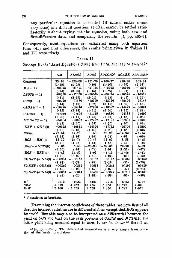
Consequently, asset equations are estimated using both equation form (41) and first differences, the results being given in Tables I1 and I11 respectively.

TABLE I1 &?wings Hamiis’ Asset Equations Using Raw Data, 1959(1) t o 196%(4)*

Constant

M(t - 1)

LSUS(t - 1)

CUS(t - 1)

OLOAN(t - 1)

CARE(t - 1)

MTDEP(t - 1)

(DEP + ONL)(t)

RUS(t)

(RUS - RM)(t)

(RUS- RLSUS)(t)

(RUS - RFD)(t)

Sl(DEP+ONL)(t)

S2(DEP+ ONL)( t ]

SS(DEP+ONL)(t]

RZ SEE D- W

AM

73.10 (1.28)

- * 00963 (. 14) *06068 (*81) .02729 (.44)

(.82)

(1.00)

(.42)

( . lo )

- .lo496

.07060

a04104

- * 00622

-22.64 (3.31) 13.39 (2.10)

9.66 (1.36) -6.43 (1.19)

- * 00233 (4.81) -00246

(3.69) - *00031

( * 44)

-9612 4.379 2.160

ALSGS

-226.08 (4.06)

-.21611 (3.28)

- * 17028 (2.36)

- ‘01186 (-19) -36216

(2.84) - 07G06

(1.11) .20837

(2.20) .lo881 (2.23) 17.26 (2.61)

(4.16) 6.66 (*81)

14.67 (3.29)

- *00166 (3.29)

- * 00262

- 00014

-26.74

(3.93)

( * 20)

* 9333 4.262 1.769

ACUS

-171.79 ( 80) - -37084

- ’66366 (2.01) - * 12199

( * 62) ~67926

(1.21) *31316

(1.18)

( .el) -24396 (1.29)

*60 ( * 02)

10.46 ( * 44)

-20.90 (.79) 6.92 ( * 40) *00162 ( * 89)

(1.46)

- * 22427

- e00663 (2.67)

(1.64)

-8481

*00409

16.466 1.768

LOLOAN

- 100.77 (1.60)

- * 12693 (1.69)

- ‘06074 (. 69) - 26726

(3.49) - *78082 (6.20)

- * 10880 (1.31)

-.17182 (1.60) *I7732

(3.00) 28-23 (3.28) 11.62 (1.66)

-32.63 (3.91) -1.19

( * 22)

(2.18) *00126

* 00248 (3.07)

- * 00047 (. 56)

*7216 6.166 2.460

ACARE

216.20 (1.20)

- -26360

- ’10676 (. 46) - a36476

(1.80) - -44479 (1.11)

- ~94188 (4.26)

- *01833

(1.24)

(. 06)

(1.88)

(. 67)

(.43)

-29707

-14.32

-8.68

29.99 (1.36)

-11.46 (a801 - 00060 (.33)

* 00100 ( * 47) - *00210 ( 96)

~6393 13.747 1.742

MTDEP

209 * 34 (2.08)

- a01297 ( e l l ) - * 16019

(1.22) - ‘28143 (2.66)

- .60091 (2.68)

- * 26693 (2.08)

- * 83603 (4.88) el7807

(2.02)

( * 60)

( * 10)

(.67)

( * 43) -00162

(1.79) eOO330

(2.74)

-7.14

-1.16

8.33

-3.41

- *00107 ( a 8 6 1

.6727 7.690 1.979

* ‘t’ statistics in brackets.

Examining the interest coefficients of these tables, we note first of all that the interest variables are in differential form except that RQS appears by itself. But this may ah0 be interpreted as a differential between the yield on CGS and that on the cash portions of CARE and MTDEP, the latter yield being assumed equal to zero. It can be shown” that if we

12 [6, pp. 219-211. The differential formulation is a very simple transforma- tion of the levels formulation.

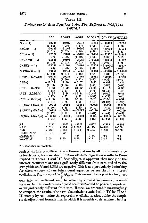
1974 PORTFOLIO CHOICE 29 TABLE I11

Savings Banks’ Asset Equations Using First Differences, 1959(2) to 1968(4)*

M(t - 1)

LSQS(1 - 1)

CQS(t - 1)

OLOAN(t - 1)

CARE(t - 1)

MTDEP(1 - 1)

(DEP + ONL)(t)

RQS(t)

(RQS - RM)(t)

(RUS- RLSQS)(t)

(RQS - RFD)(t)

Sl(DEP+ONL)(t)

S2(DEP+ ONL)( t )

S3(DEP+ ONL)( t )

RZ SEE D- W DURBIN ‘h’ DURBIN ‘1’ CIIOW ‘F’

AM

- -19136 (1.64) -20433

(1.61) a02324 (-37)

*03699 (.a41

* 19964

-02164

-el6881 (1.03)

(1.86)

(. 38)

(1.00) 3.63 ( * 48) 7.96 (a771

(-21)

- 11.68

-1.08

- ’00246 (4.90) -00237

(3-17) - * 00003

(-04)

.9217 6.613 2.238 -1.18

2.58

ALSQS

-el0627

- ‘31662 (. 96)

(2.62) .02184 (-39) -40106 (2.93)

- ‘01908 (.26) -12644

(1.31) .09623

12.96 (1.26)

(2.51) 3.38 ( 37)

10.48 (2.26)

(3.36)

(3.91)

(1.90)

- 16.72

- .00160

- *00261

- .00013 (*23)

a9063 4.994 2.106 - -60 1.90

ACQS

- -26316 (. 67) - * 10996 (-26) - -29796

(1.60) .78980

(1.63) *68308 (2.66)

- * 06368 (. 16) -07261 (*41)

-6.67 ( * 18)

34.79 (1.47)

-26.44 (*81)

26-68 (1.66) -00064 (-40) - a00787

(3.33) *00460

(2.26)

*9121 7.707 2.148

-a83 1.26

hOLOAA

*01249

el3193 (.09)

(. 89) - * 20480 (2.96) - 1 *2082’ (7.13) - -03778 (.42) -00443 (.04) a08683

(1.40) 7.08

14.08 (1.71)

(1.92) 2.73

a00038 ( * 70) .00130

(1.67) - -00021

(. 66)

-21.82

( * 29)

,8276 6-179 2.424

-2.34 1.11

ACARE

- e48309 (1.60) - .40032 (1.14)

- -33377 (2 * 04)

- *41302 (1.03)

- 1 * 4064l (6.63) - *OM40 (-31)

(3.32) - a92 (-03)

-41.16 (2.11) 46.40 (1.72)

(2.06) -00092 (. 70) -00282

(1.44) - -00302 (1.80)

-7886

*48616

-27.90

4.612 1 * 836

-91 1.43

WTDEP

*03039 (.IS)

(2-43)

(2.13)

(1 * 72)

(2.03)

(7.14) ~23763

(2.72) - -77 ( * 04) 6.36 (a461

-9.46 (-69)

-9.91 (1.22)

* 00202 (2 * 60) *00399

(3.43) - .00122 (1.22)

- a61036

- -20867

- -41082

- * 26677

- 1 * 18943

*8107 8.709 2.169

- *62 -42

* ‘1’ Statistics in brackets.

replace the interest differentials in these equations by all four interest rates in levels form, then we should obtain identical regression results to those implied in Tables I1 and 111. Secondly, i t is apparent that many of the interest coeficients are not significantly different from zero and that the own yields on ill and LSQS are negative. This is not particularly disturbing for when we look a t our behavioural equation we see that the interest coefficients, Biz, are equal to Oijajz. This means that a positive long-run

own interest coefficient may be offset by a negative cross-adjustment term so that the short-run own yield coefficient could be positive, negative, or insignificantly different from zero. Hence, we are unable meaningfully to compare the results of the two formulations embodied in Tables I1 and I11 merely by examining the regression coefficients. Also, unlike the simple stock adjustment formulation, in which it is possible to determine whether

j

30 THE ECONOMIO RECORD MAROH

the djustment speed implied by the estimates is plausible by noting the value of the coefficient of the lagged dependent variable, the adjustment mechanism in our model is very complex, with the adjustment of any one asset depending on its own and cross-adjustment coefficients and prior changes in the various assets. We must examine the stationary long-run coefficients implied by the regression estimates and thereby determine the result of the adjustment mechanism. However, before turning to these long-run coeBcients we should briefly note in Tables I1 and I11 that our least-squares estimates do indeed satisfy all our a priori constraints. Thus, the sum of coefficients relating to any one lagged asset variable across all equations is minus one, the sum of the ‘exogenous’ asset (DEP + ONL) coefficients is unity, and the sum of any particular interest rate or seasonal dummy coefficients is zero.

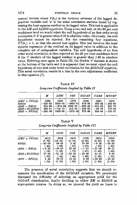
The long-run coefficients corresponding to Tables I1 and 111 are shown in Tables IV and V respectively.’ For several reasons, i t is apparent that the long-run coeflicients in Table V, derived from the first difference formulation, are markedly superior. First, the long-run coefficients of (DEP + ONL) are more plausible in the first difference formulation, implying that the savings banks ultimately invest 40 per cent and 28 per cent of any permanent increase in deposits and other net liabilities in mortgages and local and semi-government securities respectively.’ These percentages compare favourably with our a priori expectations derived from Table I, whereas the 59 per cent and 6 per cent estimates using the raw data formulation appear unrealistic. Second, the long-run interest coefficients in Table IV seem to verge on explosiveness and must be rejected as implausible. For example, the mortgage rate coefficient in the LSGS equation implies that an increase of one percentage point in this yield would increase the stock of LSGS by $1,875 m., almost doubling the existing stock as a t December 1970 (a cross-elasticity of approximately 7). Third, the long-run own interest coefficients are all positive in the first difference formulation but three of the six are implausibly negative in Table IV. These factors suggest that we should reject the estimates based on raw economic data in favour of those based on first differences.

In the lower portion of Table 111 we have shown the Durbin-Watson statistic of each equation. As is well known, when the estimating equation contains the lagged dependent variable, the statistic is biased towards 2T/T - 1, where T is the sample size. Durbin has recently suggested two tests for serial correlation when some of the regressors are lagged dependent variables [6]. The first test, which is applicable when T V ( b , ) < 1, is to

and test ‘it’ a8 a standard J1 - i V ( b l ) compute the statistic h. = a

13 These were calculated using equation (42) and involve the inversion of a 6 X 6 matrix of adjustment coefficients and then post-multiplication by the 6 X 5 matrix, B.

1 4 Whereas the dependent variable in each of the regression equations was the quarterly change in the stock of an asset, in a stationary long-run equilibrium situation such changes must be zero. Hence the interpretation of the long-run coefficients is that they show the total increase in the stock of the endogenous variable caused by a unit change in the exogenous variable.

1974 PORTFOLIO CHOICE 31 normal deviate where V ( b , ) is the variance estimate of the lagged dependent variable and ‘a’ is the serial correlation statistic found by reg- ressing the least squares residual on its lagged value. This test is applicable in the AM and ALSQS equations. Using a two-tail test, at the 95 per cent confidence level we would reject the null hypothesis of no first order serial correlation if ‘h’ is greater than 2.02 in absolute value. Obviously, the null hypothesis cannot be rejected. For the remaining four equations, TV(b , ) > 1, so that the second test applies. This test involves the least squares regression of the residual on its lagged value in addition to the complete set of independent variables. The null hypothesis of no first order serial correlation is then rejected at the 95 per cent confidence level if the ‘t’ statistic of the lagged residual is greater than 1.96 in absolute value. Referring once again to Table 111, the Durbin ‘t’ statistic is shown at the bottom of the table and it is apparent that we must reject the null hypothesis of zero first order serial correlation for the AOLOAN equation. This serial correlation results in a bias in the own adjustment coeficient in this equation [7].

.0630 2668.03 -1874.99 -714.70 1049.98

TABLE IV Long-run Coeflcients Implied by Table I I

-1679 -2683.81 2322.29 413.04

- 1276’4f

(DEP + ONL)(t) RUS(t) (RGS - R M ) ( t ) (RUS- RLSUS)(t) (RaS - RFD)(t)

M

.6886

624.98 399.81

-928.83

-286.39

I I I mas I cus I OLOAN I CARE

.0446 876.92

-662.93 -218.90 373.96

-0687 662.22

-611.08 -66.76 266.94

TABLE V Long-run Coe&ients Implied by Table 111

- (DEP + ONL)(t)

RUS(t)

( R a s - R M ) ( I )

(RUS - RLSUS) ( 1 )

(RaS - RFD)(t)

M LSUS

~2836 (13.43) 66.48 (. 96)

-40.40 (1.25)

-21.19 (. 44) 33.96 (1.28)

OLOAN

-0799 (4.64) 10.08 (.31)

-1.21 (.07)

-12.40 (-46) 4.83 (. 34)

CARE

-0674 (2.93) -6.38 (*la)

-31.06 (1.40) 41-81 (1.26)

-33.22 (1.83)

MTDEP

-0872 -383.66 201 * 79 176-84

-119.07

MTDEP

-0202 (1-08)

-29.69 (. 83) 19.11 (a961 6.63 (a211

(1.20) - 19.66

Tke presence of serial correlation suggests that we should re- examine the specification of the AOLOAN equation. We previously discussed the difficulty of selecting an appropriate yield fo r the O L O A N classification, finally deciding on either RM or RLSGS as appropriate proxies. In doing so, we ignored the yield on loans t o

32 THE ECONOMIO RECORD MARCH

authorized money market dealers, BAMM. Consequently, the model was reformulated incorporating RAMN but the results were quite disappointing as the Durbin ‘ t ’ statistic for the AOLOAN equation increased in absolute value to 2.92.

Of course, it would be possible to use the maximum-likelihood method or an iterative o r two-stage procedure suggested by Johnston [8, pp. 192-31 to remove the serial correlation from the AOLOAN equation. But then we would have to use a constrained regression estimation technique as the balance sheet constraint could no longer be satisfied using ordinary least squares, unless the iterative procedure is applied across all equations using the same value of p , the serial correlation coefficient, in each equation. This technique, however, has the effect of introducing serial correlation into the five equationa that previously had independent disturbances and is therefore unacceptable.

It is desirable to know whether the relationships estimated in Table I11 have remained stable over the sample period. Hence the sample period was split into two equal sized sub-samples and the Chow test applied, the relevant ‘P’ ratios being shown at the bottom of the table. The null hypothesis is that the estimated parameters of each equation have not changed between the two sub-samples. As the critical ‘F’ value at the 95 per cent confidence level f o r 14 and 11 degrees of freedom is 2.74, we are unable to reject the null hypothesie in any of the six equations.

Turning to the long-run interest coefficients in Table V, we note that these coefficients are not very reliable as only 6 of the 24 coefficients are larger than their standard errors. All own interest coefficients have the correct positive sign, but only the coefficients of RFD in the CARE and MTDEP equations have ‘ t ’ statistics greater than one. The insignificance of the coefficients means that we are generally unable to make statements as to whether certain assets are euhtitutes or complements, the one exception being LSGS and CARE which appear to be substitutes m both respond negatively to an increase in the yield of the other asset. This suggests that, in the long run, savings banks are not all that concerned with the different liquidity attributes of these assets, but treat them as alternative long-run investment In Part I we showed that the symmetry condition on the matrix of long-run interest coefficients only holds if asset and interest forecasting errors are assumed independent. It was therefore suggested that we adopt an unconstrained estimation procedure with respect to the symmetry conditions and test the regression coefficients to ascertain whether they are compatible with the hypothesis that the long-run cross-interest coefficients are 5ym-

16This is not necessarily inconsistent with the fact that, in the short run, CARE and MTDEP do serve a very important function in the adjustment process as we shall see later.

1974 PORTFOLIO CHOICEl 33 metrical. Because of the insignificance of the long-nm interest coefficients in Table V, it is not surprising to find that all pairs of interest coefficients overlap in the range of two standard errors and thereby are compatible with the symmetry hypothesis.

It may be possible to increase the precision of the long-run interest coefficients by eliminating insignificant variables in the respective equations but this would mean that the balance sheet constraint could not be satisfied using ordinary least squares estimation techniques. In view of the fact that we have only 39 observations, and 85 structural parameters need to be estimated, it is probably not surprising that we are unable to obtain significant coefficients for many of the variables. On the brighter side, the long-run coefficients of ( D E P + O N L ) , in Table V, are quite significant so that me can place considerable confidence in these implied coefficients.

In an attempt to improve the model’s performance it was re- estimated assuming that savings banks adjust fully in each quarter to any desired increase in their asset holdings. The explanatory power of the equations under this assumption was markedly reduced and the residuals showed evidence of positive serial correlation, indicating a likely mis-specification in the formulation and biased coefficients. For space reasons these results are not reported except to note that this procedure did increase the significance of many of the interest coefficients as we found 15 of the 24 coefficients with ‘t’ statistics greater than unity. In all cases, the sign of the cross- interest coefficients agreed with those of Table V, indicating that the results of Table V may be a useful guide in ascertaining relationships between assets. Thus, i t appears that possible complementary relationships exist between the asset combinations ( M , C A R E ) and (LSGS, CARE) while substitute relationships appear to exist between ( M , CGS) , (LSGS, C A R E ) , (LSBS, MTDEP), (CGS, CARE) and (CGS, MTDEP) . Each of the complementary relationships seems plausible as the respective asset pairs possess different liquidity and risk attributes so that they are likely to be used together to diversify the portfolio. On the other hand, CGS, MTDEP, and CARE can all serve the liquidity function so that these substitute relationships appear reasonable. The substitute relationships between (LSBS, C A R E ) and (LSGS, MTDEP) are more dificult to justify as the differing liquidity attributes would suggest complements. However, we mentioned earlier that a substantial amount of CARE and MTDEP was in the form of fixed deposits 60 that a t least this portion could be competitive with LSGS as an appropriate investment form. Finally, the substitute relationship between ( M , CGS) supports a statement made by Wallace [14, p. 2731 that ‘when a savings bank makes the decision to acquire government debt there will usually be an equivalent reduction in its ability to provide finance . . . for housing ’. B


To this point we have assumed that the volume of savings deposits is determined by the public’s demand for such assets, and hence include them as part of the predetermined asset category. This assumption is easily relaxed by including deposits as a (negative) endogenous asset and estimating 7 asset equations. Of course, we also need to add the yield on savings deposits and the lagged stock of deposits as additional independent variables. Attempts to estimate an equation for the supply of savings deposits in this manner were unsuccessful as it wm found that an insignificant positive relationship exists between savings deposits and own yield, thereby adding further support to our earlier assumption that the volume of savings deposits is demand determined.

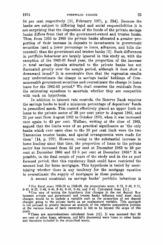
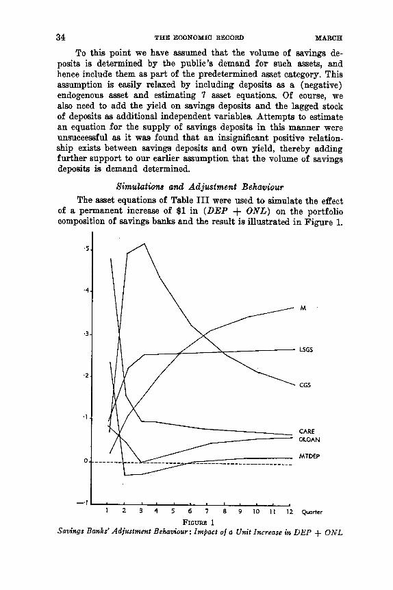
Simulations and Adjustment Behamiour The asset equations of Table I11 were used to simulate the effect

of a permanent increase of $1 in (DEP + ONL) on the portfolio composition of savings banks and the result is illustrated in Figure 1.

1

1

-1

0

-. 1

M

LSGS

CGS

CARE OLOAN

MTDEP

I , , , ,

1 2 3 4 5 6 7 8 9 10 1 1 12 Quarter

FIGURE 1 Savings Banks’ Adjustment Behuviour: Impact of a Unit Increase in DEP + ONL

1974 PORTFOLIO CHOICE 35 Initially, 72 per cent of the increase in liabilities is held as C A E E and MTDEP with 2 per cent, 10 per cent, 7 per cent and 9 per cent in M , LSGS, CGS, and OLOAN respectively. In the second period there is a dramatic shift out of C A R E and MTDEP primarily into CGS which are still relatively liquid, though somewhat higher interest yielding. There is also a substantial increase in M and LSGS in this period. In the third quarter there is a shift out of CARE and OLOAN primarily into M and LSGS, while in subsequent periods savings banks shift out of CGS into M, OLOAN and MTDEP.

Thus the model implies very realistic adjustment behaviour as the initial impact of the deposits change is felt in the highly liquid assets, CARE and MTDEP, then in the second line of liquid reserves, CGS, and finally in the illiquid assets M and LSGS. The speed of adjustment also seems quite reasonable, with 53 per cent and 91 per cent of the total adjustment in M and LSGS respectively having been accomplished after four quarters and 83 per cent and 95 per cent after eight quarters. Also, compared to the simple stock adjustment model in which assets adjust to their optimal levels from below at a k e d rate, our model implies a much more flexible and realistic adjustment mechanism. For example, we find that CGS in the first quarter is below its long-run level and finally adjusts from above. On the other hand, MTDEP and OLOAN begin above their long-run levels, decline below these levels, and ultimately ad just from below. CARE is always above its optimal level md consequently adjusts from above. This variety of adjustment behaviour is a result of the general formulation of the stock adjustment model which includes cross-adjustment effects, and is not possible in the simple stock adjustment formulation.

E x post forecasts are shown in Table VI. Comparing the mean absolute error of the forecasts with the standard error of estimates of the respective equations, we note that the LSGS, OLOAN, and MTDEP equations perform quite well. However, the CGS and CARE equations forecast poorly in 1969(2) and 1969(4) in which we find large offsetting errors in the forecasts. In the second quarter of each year, savings banks usually allow their holdings of CCS and CARE to decline in order to cover withdrawals of deposits which are normally greater than new deposits in this quarter. But in 1969(2) savings banks allowed their holdings of CARE to decline by more than twice their normal amount while stocks of CGS actually increased by $14 m. This atypical behaviour has been overlooked completely in the literature and hence we can only speculate on its possible cause. The removal of the tax rebate on Commonwealth government securities issued after 1 November 1968 reduced the relative attractiveness of these securities particularly to life insurance companies and the non-bank private sector. This may have forced several of the savings banks to support the bond market in this period. Without quarterly

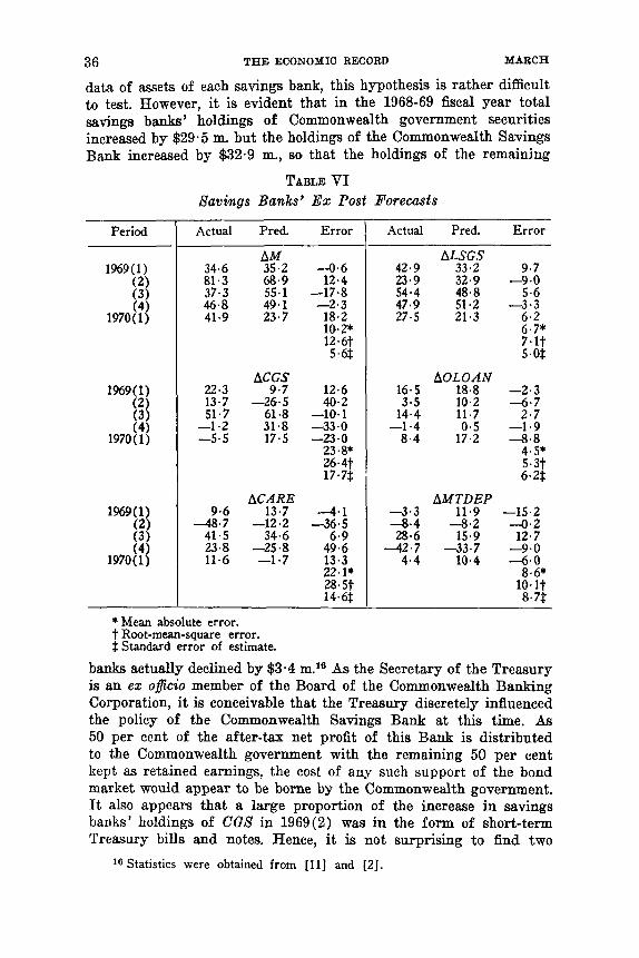
36 THE ECONOMIO RECORD MARCH

data of assets of each savings bank, this hypothesis is rather difficult to test. However, it is evident that in the 1968-69 fiscal year total savings banks' holdings of Commonwealth government securities increased by $29.5 m. but the holdings of the Commonwealth Savings Bank increased by $32.9 m., SO that the holdings of the remaining

TABLE VI Savings Banks' E x Post Porecasts

Period

1969(1) (2) (3) (4) lWO( 1)

1%9(1) (2) (3) (4)

1970( 1)

1%9(1) (2) (3 1 (4)

1970(1)

Actual Pred. Error

34.6 81.3 37.3 46.8 41.9

22.3 13.7 51.7 -1.2 -5.5

9.6 -48.7 41.5 23.8 11.6

AM 35.2 -4.6 68.9 12.4 55.1 -17.8 49.1 -2.3 23.7 18.2

1O.P 12.6t 5.6$

ACGS 9.7 12.6

-26.5 40.2 61.8 -10.1 31.8 -33.0 17.5 -23.0

23.8*

ACARE 13.7 4 . 1

-12.2 -36.5 34.6 6.9

-25.8 49.6 -1.7 13.3

22*1*

Actual Pred. Error

ALSGS 42.9 33.2 9.7 23.9 32.9 -9.0 54.4 48.8 5.6 47.9 51.2 -3.3 27.5 21.3 6-2

6.7*

AOLOAN 16.5 18.8 3.5 10.2 14.4 ii.7

-1 *4 0.5 8.4 17.2

AMTDEP -3.3 11.9 -8.4 -8.2 28.6 15.9

42.7 3 3 . 7 4.4 10.4

- . 7-lt 5.0$

-2.3 -6.7 2.7

-1.9 4 . 8 4.5* 5.3t 6*2$

-15.2 -0.2 12.7 -9.0 -6.0 8.6* l0.lt 8.7t

* Mean absolute error. t Root-mean-square error. $Standard error of estimate.

banks actually declined by $ 3 4 m.16 As the Secretary of the Treasury is an e z oficio member of the Board of the Commonwealth Banking Corporation, it is conceivable that the Treasury discretely influenced the policy of the Commonwealth Savings Bank at this time. As 50 per cent of the after-tax net profit of this Bank is distributed t o the Commonwealth government with the remaining 50 per cent kept as retained earnings, the cost of any such support of the bond market would appear to be borne by the Commonwealth government. It also appears that a large proportion of the increase in savings banks' holdings of CQS in 1969(2) was in the form of short-term Treasury bills and notes. Hence, it is not surprising to find two

16 Statistics were obtained from [ll] and [2].


quarters later, when the non-bank private sector’s demand for CGS had increased substantially, that savings banks would not replace these very short-term temporary holdings of Treasury notes. Con- sequently, we find in 1969(4) that our equations overestimate the change in CcfS and underestimate the change in CARE. It therefore appears plausible that the poor ex post forecasts of CARE and CGS in 1969(2) and 1969(4) were caused by the existence of somewhat unique circumstances and t h w cannot be attributed to any basic weakness in the behavioural equations.

Ex post forecasts of the change in the mortgage stock involve an average error almost twice the standard error of estimate. This problem is discussed in another paper [13] where it is argued that the increased use of computers by banks has allowed several of them to charge interest on their mortgages monthly, instead of half-yearly as was formerly the case. The half-yearly charge caused tremendous seasonality in the mortgage stock series but the seasonality suddenly disappears in the 1969-70 and subsequent fbcal years, thereby con- tributing to the large forecast errors.

The final test of the model involved a dynamic simulation in which (DEP + ONL), all interest rates, and initial values for each of the asset stocks, were assumed exogenously given. The value of the lagged asset stock fed into each of the asset equations waa the value which the model generated in the preceding period. Results of this simulation indicated no tendency for the errors to cumulate over time 60 that the dynamic property of the portfolio model seems sound. Earlier in the paper we suggested the possibility that in the 1962-63 fiscal year our behavioural equations may overestimate the increase in the mortgage stock with an offsetting error in the CGS equation. The dynamic simulation errors were compatible with this hypothesis, so it appears that future research on portfolio behaviour of savings banks should include the proportion of total deposits attracted by the private banks as an explanatory variable. We also mentioned the possibility that, in the e z post forecast periods 1969 (1) to 1970 (l), our behavioural equations may overestimate the increase in mortgages as the re-datory limit of 35 per cent of depositors’ funds invested in private sector loans was rapidly being approached. Because of the changing seasonality pattern in the mortgage stock, however, we are unable to investigate this possibility.

Conclusion Generally speaking, the results of this study lend empirical

support to the general stock adjustment formulation: it appears that portfolio decisions do take account of liquidity and, to a lesser extent, of profitability attributes of the various assets. Also, the statistical significance of many of the cross-adjustment coefficients indicate that asset adjustments are not performed independently as is generally

38 THE ECONOMIC RECORD MARCH 1974

implied by the simple stock adjustment formulation. Moreover, the general stock adjustment formulation produced a plausible and extremely flexible adjustment mechanism, proceeding from the highly liquid assets, to CGS, and ultimately to the illiquid assets.

The least satisfactory aspect of the regression results is the finding that the long-run interest coefficients are generally insignificant a t the 95 per cent confidence level. There are several possible explanations for this finding, the most obvious perhaps being the fact that interest rates have generally moved in the same direction and a t much the same time. However, while such multicollinearity produces large standard errors of estimates, it does not lead to biased coefficients, ceter is paribus. Secondly, the inclusion of the Common- wealth and State owned banks introduces the possibility that social and political factors could outweigh profitability factors in their portfolio choice. A disaggregated study of private banks v i s - h i s public banks’ portfolio choice appears desirable but at the present time quarterly asset data are not available on this basis. Finally, it is possible that the restrictions on portfolio choice imposed by the Reserve Bank could have severely limited the responsiveness of savings banks to interest rate changes. Thus i t may take huge shifts in relative interest rates if the Reserve Bank wishes to divert funds from one use to another. It should be emphasized, however, that the portfolio restrictions are of a general form and that there is ample opportunity for banks to switch between CARE, MTDEP, CGS, LSGS and OLOAN in response t o changing interest differentials. Failure to do 60 could reflect a lack of dynamic investment manage- ment rather than Reserve Bank controls.

IAN SHARPE University of Sydney

REFERENCES [ l ] Christ, C. F., Econometric Models and Methods (Wiley, New York, 1966). [2 ] Commonwealth Banking Corporation, Annual Reports. [3] Commonwealth Bureau of Census and Statistics, Banking and Currency. [41 [S] Durbin, H., ‘Testing for Serial Correlation in Least-Squares Regression

When Some of the Regressors Are Lagged Dependent Variables’, Econo- metrica, Vol. 38, May 1970.

[6] Goldberger, A. S., Econometric Theory (Wiley, New York, 1964). [7] Griliches, Z., ‘A Note on Serial Correlation Bias in Estimates of Distributed

Lags’, Econometrica, Vol. 29, January 1961. [8] Johnston, J., Econometric Methods JMcGraw-Hill, New York, 1963). [9] Kmenta, J., Elemerrts of Econometrrcs (Macmillan, New York, 1971).

, Oficial Year Book of the Commonwealth of Australia.

[ 101 Reserve Bank of Australia, Reserve Bank of Australia : Functions and Opera-

[111 ~ , Statrstrcal Bulletin. [12] Rose, P. J., Australiw Securities Markets (Cheshire, Melbourne, 1969). [13] I. G. Sharpe, ‘A Mortgage Model: Some Theoretical and Empirical Results

as Applied to Australian Savings Banks’, unpublished manuscript, Univer- sity of Sydney, 1972.

[14] Wallace, R. H., ‘The Australian Savings Banks’, in R. R. Hirst and R. H. Wallace (eds.), Studies in the Australian Capital Market (Cheshire, Mel- bourne, 1964).

tiom (Sydney,. !969).

Documents

A Quarterly Econometric Model of Portfolio Choice — Part II: Portfolio Behaviour of Australian Savings Banks