Embed Size (px)
Citation preview
1
A Quick Guide to the Self-consistent Field Theory in
Polymer Physics
Yi-Xin Liu
2011.2.28
Equation Section 1Introduction
The self-consistent field theory (SCFT) for many-chain systems is obtained by imposing a
mean-field approximation to simplify the statistical field theories. The statistical field theories can
be constructed from the particle-based model by carrying out a particle-to-field transformation.
The general approach for a particle-to-field transformation is to invoke formal techniques related
to Hubbard-Stratonovich transformations, which have the effect of decoupling interactions among
particles (or polymer segments) and replacing them with interactions between the particles and
one or more auxiliary fields.
(a)
(b)
(c)
Figure 1
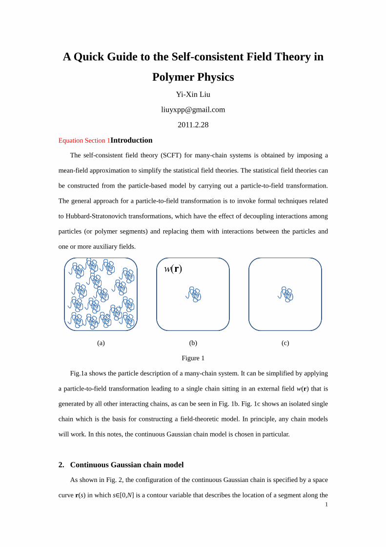
Fig.1a shows the particle description of a many-chain system. It can be simplified by applying
a particle-to-field transformation leading to a single chain sitting in an external field w(r) that is
generated by all other interacting chains, as can be seen in Fig. 1b. Fig. 1c shows an isolated single
chain which is the basis for constructing a field-theoretic model. In principle, any chain models
will work. In this notes, the continuous Gaussian chain model is chosen in particular.
2. Continuous Gaussian chain model
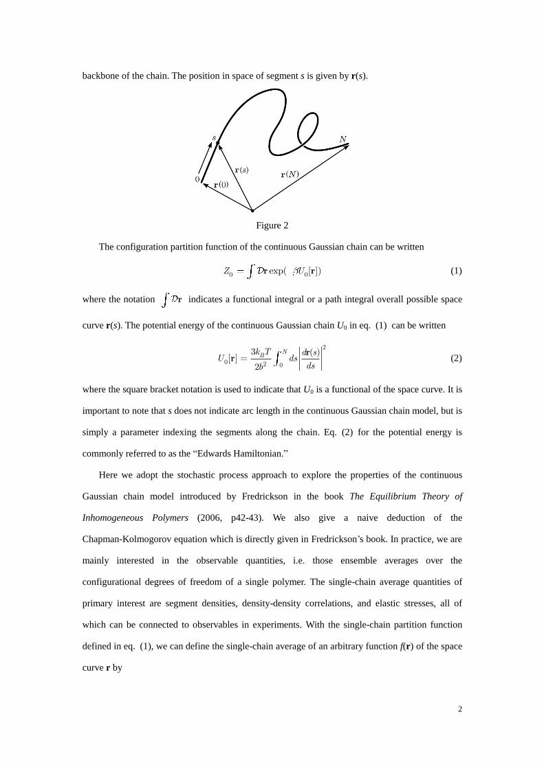
As shown in Fig. 2, the configuration of the continuous Gaussian chain is specified by a space
curve r(s) in which s∈[0,N] is a contour variable that describes the location of a segment along the
2
backbone of the chain. The position in space of segment s is given by r(s).
Figure 2
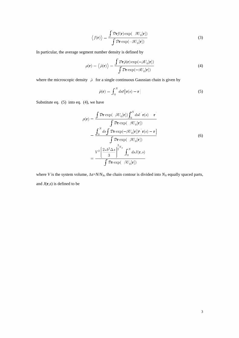
The configuration partition function of the continuous Gaussian chain can be written
0 0exp( [ ])Z Ur r (1)
where the notation r indicates a functional integral or a path integral overall possible space
curve r(s). The potential energy of the continuous Gaussian chain U0 in eq. (1) can be written
2
0 2 0
3 ( )[ ]
2
NBk T d s
U dsdsb
rr (2)
where the square bracket notation is used to indicate that U0 is a functional of the space curve. It is
important to note that s does not indicate arc length in the continuous Gaussian chain model, but is
simply a parameter indexing the segments along the chain. Eq. (2) for the potential energy is
commonly referred to as the “Edwards Hamiltonian.”
Here we adopt the stochastic process approach to explore the properties of the continuous
Gaussian chain model introduced by Fredrickson in the book The Equilibrium Theory of
Inhomogeneous Polymers (2006, p42-43). We also give a naive deduction of the
Chapman-Kolmogorov equation which is directly given in Fredrickson’s book. In practice, we are
mainly interested in the observable quantities, i.e. those ensemble averages over the
configurational degrees of freedom of a single polymer. The single-chain average quantities of
primary interest are segment densities, density-density correlations, and elastic stresses, all of
which can be connected to observables in experiments. With the single-chain partition function
defined in eq. (1), we can define the single-chain average of an arbitrary function f(r) of the space
curve r by
3
0
0
( )exp( [ ])( )
exp( [ ])
f Uf
U
r r rr
r r (3)
In particular, the average segment number density is defined by
0
0
(̂ )exp( [ ])ˆ( ) ( )
exp( [ ])
U
U
r r rr r
r r (4)
where the microscopic density ˆ for a single continuous Gaussian chain is given by
0
(̂ ) ( )Nds sr r r (5)
Substitute eq. (5) into eq. (4), we have
0 0
0
00
0
32 2
2
0
0
exp( [ ]) ( )( )
exp( [ ])
exp( [ ]) ( )
exp( [ ])
2( , )
3
exp( [ ])
N
N
N
NN
U ds s
U
ds U s
U
b sV dsJ s
U
r r r rr
r r
r r r r
r r
r
r r
(6)
where V is the system volume, s=N/NN, the chain contour is divided into NN equally spaced parts,
and J(r,s) is defined to be
4
32
2
2 2 20
32 2
2
2 2 2 20
2 2
( ')1 3 3( , ) exp ' ( )
'2 2
( ') ( ')1 3 3 3exp ' '
' '2 2 2
( )
1 3
2
N
N
NN
Ns N
s
d sJ s ds s
dsV b s b
d s d sds ds
ds dsV b s b b
s
V b s
rr r r r
r rr
r r3
2 22
2 20
32 2
2
2 2 2 20
( ') ( ')3 3exp ' '
' '2 2
( ) 1
( ') ( ')1 3 3 3exp ' '
' '2 2 2
( ) ( ) (
N
N
Ns N
s
Ns N
s
d s d sds ds
ds dsb b
s
d s d sds ds
ds dsV b s b b
s d s s
r rr
r r
r rr
r r r r3
22
2 20
32( )
2
2 2
)
( ')1 3 3exp ' ( )
'2 2
( ')1 3 3exp ' ( )
'2 2
1 1( , ) ( , )
1 1( , )
s
N s
Ns
N NN
s
d sds s
V dsb s b
d sds s
V dsb s b
q s q N sV V
q s qV V
r
rr r r
rr r r
r r
r *( , )sr
(7)
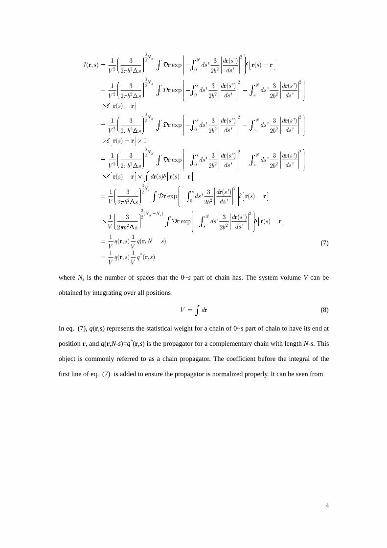
where Ns is the number of spaces that the 0~s part of chain has. The system volume V can be
obtained by integrating over all positions
V dr (8)
In eq. (7), q(r,s) represents the statistical weight for a chain of 0~s part of chain to have its end at
position r, and q(r,N-s)=q*(r,s) is the propagator for a complementary chain with length N-s. This
object is commonly referred to as a chain propagator. The coefficient before the integral of the
first line of eq. (7) is added to ensure the propagator is normalized properly. It can be seen from
5
32
2
2 20
32
2
2 20
3
2
2
1( , )
( ')1 3 3exp ' ( )
'2 2
( ')1 3 3exp ' ( )
'2 2
1 3
2
s
s
s
Ns
Ns
N
d q sV
d sd ds sV dsb s b
d sds d s
V dsb s b
V b s
r r
rr r r r
rr r r r
r2
20
3
2 212 2
0 13
2 2 20 0 1 1 1 22 2 2
( ')3exp '
'2
1 3 3exp
2 2
1 3 3 3exp exp
2 2 2
s ss
s
s
s
N NN
j i ij i
N
N
d sds
dsb
dV b s b s
d d dV b s b s b s
r
r r r
r r r r r r r
2
1 12
3
2 2
2 2
3
2 2 2 22 2
2
3exp
2
1 3 3exp
2 2
1 3 3exp ( )
2 2
1 3
2
s s s
s s
s
s s
s
N N N
N N
N
N N
N
db s
d dV b s b s
dxdydz x y z dV b s b s
VV b
r r r
r r r
r
3
2 2 2 22 2 2
1 1 132 2 22 2 22
2
3 3 3exp exp exp
2 2 2
3 2 2 2
3 3 32
s s
s
N N
N
dx x dy y dz zs b s b s b s
b s b s b s
b s
332 22
2
3 2
321
s
ss
N
NNb s
b s
(9)
To calculate the single-chain partition function, just integrate J(r,s) respect to r and multiply
it with an appropriate coefficient. It can be seen from
32 2
2
3 322 2 22
2 2 20
2
20
2( , )
3
( ')2 1 3 3exp ' ( )
3 '2 2
( ')3exp '
'2
N
N N
N
N NN
N
b sV d J s
d sb sV d ds s
dsV b s b
d sds d
dsb
r r
rr r r r
rr r r
2
20
0
0
( )
( ')3exp '
'2
exp( [ ])
N
s
d sds
dsb
U
Z
r
rr
r r
(10)
6
Therefore, inserting eq. (7) and eq. (10) into eq. (6), we can evaluate average segment number
density as
0( , ) ( , )
( ) ( )( , ) ( , )
Ndsq s q N s
d q s q N s
r rr r
r r r (11)
It will be clear later that it is convenient to define a normalized single-chain partition function Q
as
0
( ) 0( ) 0
Z wQ w
Z
rr (12)
In this case, the external field is 0 everywhere. Since Z[w(r)=0] is just Z0, eq. (12) is reduced to
( ) 0 1Q w r (13)
As shown in eq. (45), Z0 can be evaluated analytically,
32 2
02
3
NNb sZ V (14)
Insert eq. (14) into eq. (10), we have
0( ) 0 ( , )Z w VZ d J sr r r (15)
Thus, the single-chain partition function can be expressed as
1
( ) 0 ( , ) ( , )Q w d q s q N sV
r r r r (16)
with J replaced by the next to last line of eq. (7). And the average segment density can be written
as
0
1( ) ( , ) ( , )
[ ( )]
Ndsq s q N s
VQ wr r r
r (17)
by inserting eq. (16) into eq. (11). Actually, eq. (16) and eq. (17) is at least valid for any linear
polymers as long as the continuous Gaussian chain model is used.
The propagator q is a central quantity in statistical field theory. The ensemble averages and
the single-chain partition function can be derived from it. Below we will derive an equation to
compute it conveniently.
First, we explicitly write the chain propagator q in the form:
7
32
2
2 200
( ')3 3( , ) ( )exp ' ( )
'2 2
sN s s
t
d sq s d t ds s
dsb s b
rr r r r (18)
where we use the discrete approach to define a path integral, such as
0 0
( )sNs
it i
d t dr r r (19)
Note the short hand notation for functional differential is used, and it should be understood that
keeping the continuous form of U0 in eq. (18) instead of discretization one is just for clarity in
presentation (See Fredrickson, 2006 for more details about the definition and description of the
path integral).
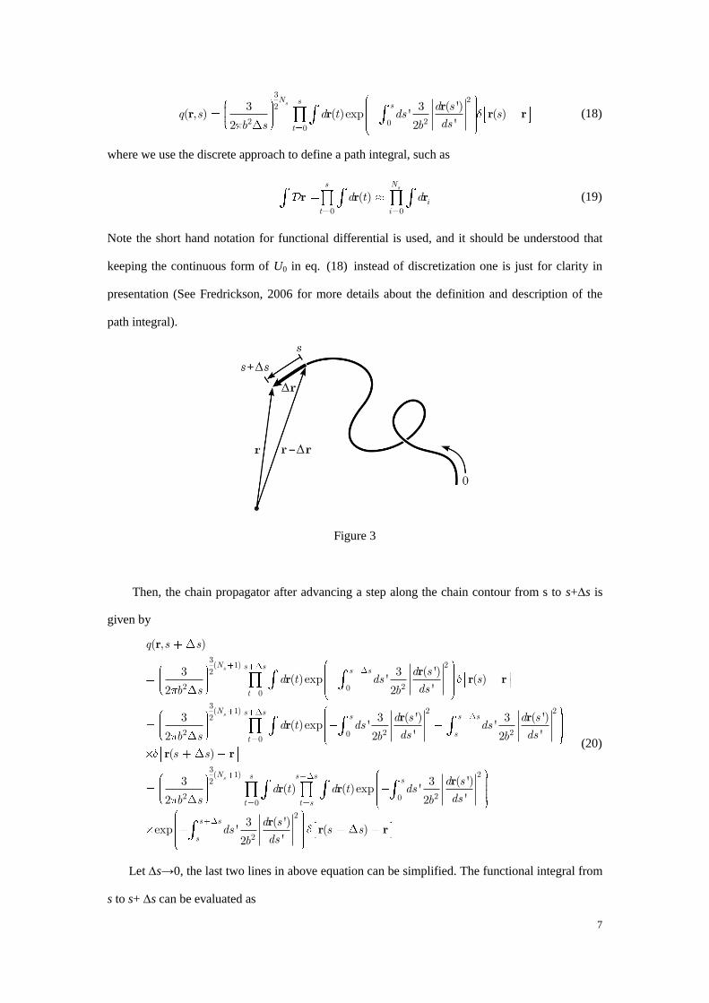
Figure 3
Then, the chain propagator after advancing a step along the chain contour from s to s+s is
given by
32( 1)
2
2 200
32 2( 1)
2
2 2 20
( , )
( ')3 3( )exp ' ( )
'2 2
( ') ( ')3 3 3( )exp ' '
' '2 2 2
s
s
N s s s s
t
Ns s s
st
q s s
d sd t ds s
dsb s b
d s d sd t ds ds
ds dsb s b b
r
rr r r
r rr
0
32( 1)
2
2 200
2
2
( )
( ')3 3( ) ( )exp '
'2 2
( ')3exp ' ( )
'2
s
s s
N s s s s
t t s
s s
s
s s
d sd t d t ds
dsb s b
d sds s s
dsb
r r
rr r
rr r
(20)
Let s→0, the last two lines in above equation can be simplified. The functional integral from
s to s+s can be evaluated as
8
( )
1 2( ) ( ) ( )
( )
( )
s s
t s
d t
d s s d s s d s sn n
d s s
d s
d
r
r r r
r
r r
r
(21)
From the second line to the third line, only one step is needed to advance from s to s+s when s
is sufficiently small. From the fourth line to the fifth line, r(s) is constant for a certain
configuration. Note that the range of possible values of r is (-∞,+∞) because the integrand
approach 0 when r→∞. The delta functional can be evaluated as
( ) ( )
( ) ( )
s s s
s
r r r r r
r r r (22)
And the second part of the potential energy can be evaluated as
2
2
2
2
2
2
2
2 2
22
( ')3'
'2
( )3
2
( ) ( )3
23
23
2
s s
s
d sds
dsb
d s
dsb
s s ss
sb
sb s
b s
r
r
r r
r
r
(23)
Through insertion of eq.(19), (20), and (21) into eq. (18), we can find the Chapman-Kolmogorov
equation given in Fredrickson’s book (eq. 2.58):
32( 1)
2 22 2 20
0
32
2
2 20
( , )
( ')3 3 3( ) exp ' exp
'2 2 2
( ) ( )
( ')3 3( )exp '
'2 2
s
s
N s s
t
Ns
q s s
d sd t d ds
dsb s b b s
s
d sd d t ds
dsb s b
r
rr r r
r r r
rr r
0
3
2 22 2
3
2 22 2
( ) ( )
3 3exp
2 2
3 3( , ) exp
2 2( ) ( , )
s
t
s
b s b s
d q sb s b s
d q s
r r r
r
r r r r
r r r r
(24)
9
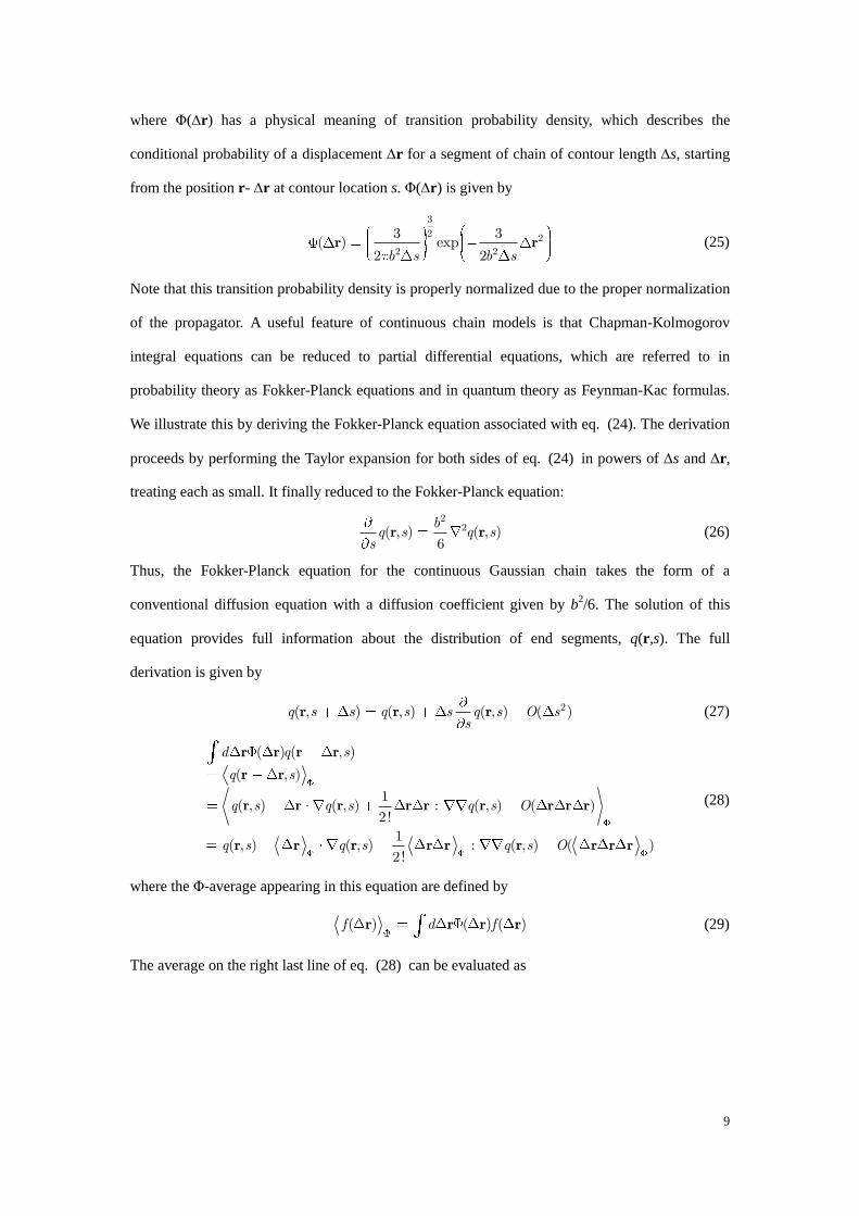
where Φ(r) has a physical meaning of transition probability density, which describes the
conditional probability of a displacement r for a segment of chain of contour length s, starting
from the position r-r at contour location s. Φ(r) is given by
3
2 22 2
3 3( ) exp
2 2b s b sr r (25)
Note that this transition probability density is properly normalized due to the proper normalization
of the propagator. A useful feature of continuous chain models is that Chapman-Kolmogorov
integral equations can be reduced to partial differential equations, which are referred to in
probability theory as Fokker-Planck equations and in quantum theory as Feynman-Kac formulas.
We illustrate this by deriving the Fokker-Planck equation associated with eq. (24). The derivation
proceeds by performing the Taylor expansion for both sides of eq. (24) in powers of s and r,
treating each as small. It finally reduced to the Fokker-Planck equation:
2
2( , ) ( , )6
bq s q ssr r (26)
Thus, the Fokker-Planck equation for the continuous Gaussian chain takes the form of a
conventional diffusion equation with a diffusion coefficient given by b2/6. The solution of this
equation provides full information about the distribution of end segments, q(r,s). The full
derivation is given by
2( , ) ( , ) ( , ) ( )q s s q s s q s O ss
r r r (27)
( ) ( , )
( , )
1( , ) ( , ) : ( , ) ( )
2!1
( , ) ( , ) : ( , ) ( )2!
d q s
q s
q s q s q s O
q s q s q s O
r r r r
r r
r r r r r r r r r
r r r r r r r r r
(28)
where the Φ-average appearing in this equation are defined by
( ) ( ) ( )f d fr r r r (29)
The average on the right last line of eq. (28) can be evaluated as
10
3
2 22 2
3
2 2 22 2
322 2
2 2
3 3exp
2 2
1 3 3( )exp
2 2 2
1 3 2 3exp
2 32 20
db s b s
db s b s
b s
b s b s
r r r r
r r
r
(30)
2
3
b sr r r r (31)
Insert eq. (30) and (31) into eq. (28), and equal it to eq. (27), we find
2
2 2( , ) ( , ) ( ) ( , ) ( , ) ( )6
bq s s q s O s q s s q s O
sr r r r r r r (32)
Let s→0, eq. (26) is finally obtained.
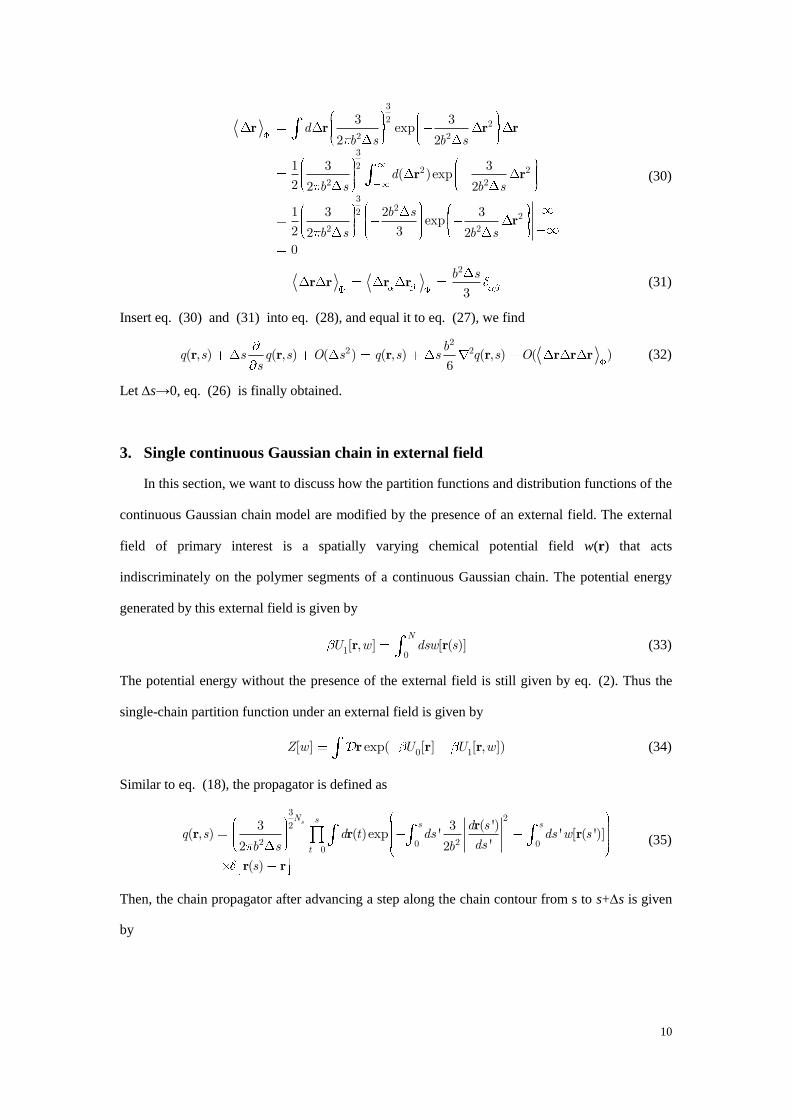
3. Single continuous Gaussian chain in external field
In this section, we want to discuss how the partition functions and distribution functions of the
continuous Gaussian chain model are modified by the presence of an external field. The external
field of primary interest is a spatially varying chemical potential field w(r) that acts
indiscriminately on the polymer segments of a continuous Gaussian chain. The potential energy
generated by this external field is given by
1 0[ , ] [ ( )]
NU w dsw sr r (33)
The potential energy without the presence of the external field is still given by eq. (2). Thus the
single-chain partition function under an external field is given by
0 1[ ] exp( [ ] [ , ])Z w U U wr r r (34)
Similar to eq. (18), the propagator is defined as
32
2
2 20 00
( ')3 3( , ) ( )exp ' ' [ ( ')]
'2 2
( )
sN s s s
t
d sq s d t ds ds w s
dsb s b
s
rr r r
r r
(35)
Then, the chain propagator after advancing a step along the chain contour from s to s+s is given
by
11
3( 1)
2
20
2
20 0
2
2
3( , ) ( ) ( )
2
( ')3exp ' ' [ ( ')]
'2
( ')3exp '
'2
exp ' [ ( ')] ( )
sN s s s
t t s
s s
s s
s
s s
s
q s s d t d tb s
d sds ds w s
dsb
d sds
dsb
ds w s s s
r r r
rr
r
r r r
(36)
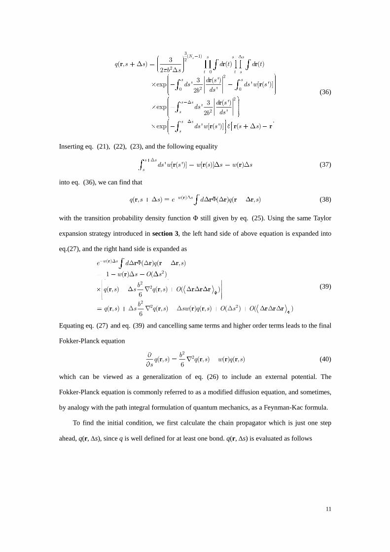
Inserting eq. (21), (22), (23), and the following equality
' [ ( ')] [ ( )] ( )s s
sds w s w s s w sr r r (37)
into eq. (36), we can find that
( )( , ) ( ) ( , )w sq s s e d q srr r r r r (38)
with the transition probability density function Φ still given by eq. (25). Using the same Taylor
expansion strategy introduced in section 3, the left hand side of above equation is expanded into
eq.(27), and the right hand side is expanded as
( )
2
22
22 2
( ) ( , )
1 ( ) ( )
( , ) ( , ) ( )6
( , ) ( , ) ( ) ( , ) ( ) ( )6
w se d q s
w s O s
bq s s q s O
bq s s q s sw q s O s O
r r r r r
r
r r r r r
r r r r r r r
(39)
Equating eq. (27) and eq. (39) and cancelling same terms and higher order terms leads to the final
Fokker-Planck equation
2
2( , ) ( , ) ( ) ( , )6
bq s q s w q ssr r r r (40)
which can be viewed as a generalization of eq. (26) to include an external potential. The
Fokker-Planck equation is commonly referred to as a modified diffusion equation, and sometimes,
by analogy with the path integral formulation of quantum mechanics, as a Feynman-Kac formula.
To find the initial condition, we first calculate the chain propagator which is just one step
ahead, q(r, s), since q is well defined for at least one bond. q(r, s) is evaluated as follows
12
3
2
2
2
20 0
3
2
2
2
2
3( , ) (0) ( )
2
( ')3exp ' ' [ ( ')] ( )
'2
3(0) ( )
2
( ) (0)3exp [ ( )] ( )
2
s s
q s d d sb s
d sds ds w s s
dsb
d d sb s
ss sw s s
sb
r r r
rr r r
r r
r rr r r
32
2
2 2
3
2 2( )2 2
( )
(0)3 3(0)exp ( )
2 2
3 3(0) exp (0)
2 2sw
sw
d s swsb s b
e db s b s
e
r
r
r rr r
r r r
(41)
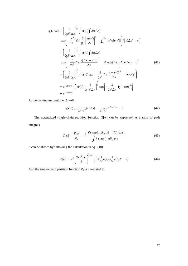
At the continuum limit, i.e. s→0,
( )
0 0( ,0) lim ( , ) lim 1sw
s sq q s e rr r (42)
The normalized single-chain partition function Q[w] can be expressed as a ratio of path
integrals
0 1
0 0
exp( [ ] [ , ])[ ][ ]
exp( [ ])
U U wZ wQ w
Z U
r r r
r r (43)
It can be shown by following the calculation in eq. (10)
32 2
2 2 1 1[ ] ( , ) ( , )
3
NNb sZ w V d q s q N s
V Vr r r (44)
And the single-chain partition function Z0 is integrated to
13
02
20
212
0 1
2 20 0 1 1 1 22 2
2
1 12
( ')3exp '
'2
3exp
2
3 3exp exp
2 23
exp2
NN
N
N N N
N
NN
j i ij i
N
N N N
Z
d sds
dsb
db s
d d db s b s
db s
rr
r r r
r r r r r r r
r r r
2
2
2 2 22
2 2 22 2 2
2
3exp
2
3exp ( )
2
3 3 3exp exp exp
2 2 2
2
3
N
N
s
N
N
N
N
N
N
N
d db s
dxdydz x y z db s
V dx x dy y dz zb s b s b s
b sV
r r r
r
1 1 12 22 2 2
32 2
2 2
3 3
2
3
N
N
N
N
b s b s
b sV
(45)
Therefore, the normalized partition function in the term of propagator q is obtained by substituting
eq. (44) and (45) into (43):
1
[ ] ( , ) ( , )Q w d q s q N sV
r r r (46)
Particularly, let s=0 and invoke the initial condition given by eq. (42), we have
1
[ ] ( , )Q w d q NV
r r (47)
The modified diffusion equation together with the above equation fully describes the statistical
mechanics of the continuous Gaussian chain in an external potential w(r).
With the definition of chain propagator, it is easy to verify that the average segment number
density is still given by eq. (11):
14
0
32
2
2 20 0 00
3( )
2
2 2
( , ) ( , )
( , ) ( , )
( ')1 3 3( )exp ' ' [ ( ')] ( )
[ ( )] '2 2
( '3 3( )exp '
2 2
s
N s
N
N sN s s
t
N N
dsq s q N s
d q s q N s
d sds d t ds ds w s s
VQ w dsb s b
d sd t ds
b s b
r r
r r r
rr r r r
r
rr
2
0 00
32
202 20 0 0
0
3( )
2
2
)' [ ( ')] ( )
'
( ')3 3( )exp ' ' [ ( ')] ( )
'2 2
3(
2
s
N s
N s N s N s
t
N sN s s
t
N N
ds w s sds
Z d sds d t ds ds w s s
VZ dsb s b
d tb s
r r r
rr r r r
r2
2
2
20 0 00
2
2 0
( ')3)exp ' ' [ ( ')] ( )
'2
( ')1 3( )exp ' ' [ ( ')] ( )
'2
( ')1 3( )exp ' ' [ ( ')]
'2
N N N
s st s
NN N N
t
N
d sds ds w s s
dsb
d sds d t ds ds w s s
Z dsb
d sd t ds ds w s
Z dsb
rr r r
rr r r r
rr r
0 00
2
20 00
2
20 0
2
2
( )
( ')1 3( ) ( )exp ' ' [ ( ')]
'2
( ')3( )exp ' ' [ ( ')]
'2
( ')3exp '
'2
N N N
t
N N N
t
N N
ds s
d sd t ds ds w s
Z dsb
d sds ds w s
dsb
d sds
dsb
r r
rr r r
rr r r
rr
0 0' [ ( ')]
( ) ( )
N Nds w sr
r r
(48)
From first equal sign to the second equal sign, eq. (43) is used, from the second equal sign to the
third equal sign eq. (45) is used, and from the fifth equal sign to the sixth equal sign eq. (34) is
used. Substituting eq. (46) into above equation, the average segment density can be evaluated
using
0
1( ) ( ) ( , ) ( , )
[ ( )]
Ndsq s q N s
VQ wr r r r
r (49)
4. Many-chain model for two-bead chains
In previous two sections, we deal with single-chain systems. From now on, we start to analyze
the properties of many-chain systems. To construct a field theory for many-chain system, the
particle-to-field transformation should be performed. The most important mathematical tool
during the particle-to-field transformation is the delta functional, which is defined as
15
[ ] [ ] [ ]F F (50)
for any functional F[]. The delta functional can be viewed as an infinite-dimensional version of
the Dirac delta function that vanishes unless the fields (r) and ( )r are equal at all points r in
the domain of interest. A useful complex exponential representation of the delta functional can be
developed by temporarily discretizing space using Mg grid points according to
1 1 1 2 2 2
1
( )[ ( ) ( )]
1
( )[ ( ) ( )] ( )[ ( ) ( )]1 2
( )[ (
[ ] [ ( ) ( )]
[ ( ) ( )]
1( )
2
1( ) ( )
2
( )
g
g
i i i
g
M Mg
g
M
i iiM
iwi
iM
iw iw
iw
M
dw e
dw e dw e
dw e
r
r r r
r r r r r r
r r
r r
r r
r
r r
r
1
) ( )]
( )[ ( ) ( )]
1 2
( )[ ( ) ( )]
1( ) ( ) ( )
2
Mg g
Mg
g j j jj
g
M i w
M
i d w
dw dw dw e
w e
r
r r r
r r r r
r r r
(51)
The third line of the above expression follows from the application of the representation of the
one-dimensional delta function [ ( ) ( )]i ir r at grid ri. The final expression results from
restoring the continuum description and can be viewed as a formal definition of the functional
integral w over the auxiliary field w(r). It is important to note that w(r) is a real scalar field
and that the functional integral in eq. (51) is taken along the whole real axis at each r.
Now, it is ready for us to examine the simplest many-chain model for diblock copolymers:
two-bead model. In two-bead model, there are n chains in the system. Each chain has two beads A
and B connected by a spring. The potential energy of this system has two sources of contribution:
the intramolecular, short-ranged interferences and the intermolecular interactions among segments.
The first energetic contribution is just sum of spring energies stored in all chains:
22
01
( )2
nn
Ai Bij
U r r r (52)
where r2n
=(r1,r2,…,r2n) denotes the set of 2n bead positions, and is the spring constant. The
second energetic contribution originates from the interaction between any of two beads in the
system, whose general form is given by
16
21 , ' '
1 1 , ' ,
, ' ', , '
1( ) ( )
2
1( )
2
n nn
j kj k AB AB
j kj k
U u
u
r r r
r r
(53)
where u(r) is the familiar pair potential function. The factor of 1/2 in the expression corrects for
the counting of each pair of particles twice in the double sum. If we define the microscopic density
operators for bead A and bead B as
1
( ) ( )n
jj
r r r (54)
where denotes either A or B. With this definition, it follows that
21 , ' '
, '
1( ) ' ( ) ( ' ) ( ')
2nU d d ur r r r r r r (55)
The equality can be seen from
, ' ', '
, ' ', '
' , ', '
' , ', '
' , '
1' ( ) ( ') ( ')
2
1' ( ) ( ') ( ')
2
1' ( ') ( ') ( )
2
1' ( ') ( ') ( )
2
1' ( ') ( ')
2
jj
jj
jj
jj
d d u
d d u
d d u
d d u
d u
r r r r r r
r r r r r r r
r r r r r r r
r r r r r r r
r r r r, '
' , ', '
' , ', '
, ' ', '
, ' ', '
, ' ', , '
1' ( ') ( ')
2
1' ( ) ( ')
2
1' ( ') ( )
2
1( )
2
1( )
2
jj
k jj k
j kj k
j kj k
j kj k
d u
d u
d u
u
u
r r r r
r r r r r
r r r r r
r r
r r (56)
In the two-bead model, the interaction energies between segments of different types separated by
distance 'r r are:
, ( ' ) ( ')AA AAu ur r r r (57)
, ( ' ) ( ')B B BBu ur r r r (58)
17
, ,( ' ) ( ' ) ( ')AB B A ABu u ur r r r r r (59)
where AAu , BBu , ABu are the intersegment excluded volumes arising from the short range
interactions, is the Dirac delta function. It follows that eq. (55) can be reduced to
21 ,
,
,
,
1( ) ' ( ) ( ' ) ( ')
21
' ( ) ( ' ) ( ')21
' ( ) ( ' ) ( ')21
' ( ) ( ' ) ( ')21
' ( ) ( ') ( ')21
' ( ) ( ')2
nA AA A
A AB B
B B A A
B B B B
A AA A
A AB
U d d u
d d u
d d u
d d u
d d u
d d u
r r r r r r r
r r r r r r
r r r r r r
r r r r r r
r r r r r r
r r r r r ( ')
1' ( ) ( ') ( ')
21
' ( ) ( ') ( ')21
( ) ' ( ') ( ')21
( ) ' ( ') ( ')21
( ) ' ( ') ( ')21
( ) ' ( ')2
B
B AB A
B BB B
A AA A
A AB B
B AB A
B BB B
d d u
d d u
d d u
d d u
d d u
d d u
r
r r r r r r
r r r r r r
r r r r r r
r r r r r r
r r r r r r
r r r r r
2 2
( ')
1 1( ) ( ) ( ) ( )
2 21 1
( ) ( ) ( ) ( )2 2
( ) ( ) ( ) ( )2 2
AA A A AB A B
AB B A BB B B
AA BBA B AB A B
u d u d
u d u d
u ud d u d
r
r r r r r r
r r r r r r
r r r r r r r
(60)
By applying the incompressible condition 0 ( ) ( )A Br r , the first integral in the last line of
above equation can be evaluated as
18
2
2 2 2
2 2 20
20
20
( )
1 1 1( ) ( ) ( ) ( ) ( ) ( )
2 2 21 1
( ) ( ) ( ) ( )2 21 1
( ) ( ) ( ) ( ) ( ) ( )2 21
( ) ( )2
A
A B B A B A
A B A B
A B A B A B
A B
d
d
d
d
d
r r
r r r r r r r
r r r r r
r r r r r r r
r r r 0
20 0 0
20 0 0
20 0 0
1 1
0 0 0
1( ) ( )
21
( ) ( ) ( ) ( )2
( ) ( ) ( ) ( )2 2 2
( ) ( ) ( ) ( )2 2 2
2
2 2 2
A B
A B A B
A B A B
n n
Aj Bj A Bj j
d d
d d d d
Vd d d
n n nd
r r
r r r r r r
r r r r r r r r
r r r r r r r r r
r
0
( ) ( )
( ) ( )
A B
A Bn d
r r
r r r
(61)
The second integral is evaluated similary,
20( ) ( ) ( )B A Bd n dr r r r r (62)
Substituting eq (61) and (62) into eq (60), we have
21
0
0
0
0 0
( )
( ) ( )2
( ) ( )2
( ) ( )
2( ) ( )
2 2
( ) ( )2
n
AAA B
BBA B
AB A B
AB AA BB AA BBA B
AA BBA B
U
un d
un d
u d
u u u u ud n
u uv d n
r
r r r
r r r
r r r
r r r
r r r
(63)
where v0=1/0 is the volume of a statistical segment (here the volume of the bead), and is just
the Flory-Huggins interaction parameter:
0
2
2AB AA BBu u u
v (64)
The constant term in eq 63 can be ignored since it has no thermodynamic consequence. Finally we
have
21 0( ) ( ) ( )n
A BU v dr r r r (65)
The canonical partition function for the two-bead system has the usual form
19
2 2 20 1 03 2
1exp ( ) ( ) ( ) ( )
!( )n n n
A BnT
Z d U Un
r r r r r (66)
where 1/n! corrects the fact of n indistinguishable two-bead chains and
2
T
B
h
mk T (67)
is the thermal wavelength, m is the mass of an atom, and h is the Planck constant. The object
0 ( ) ( )A Br r denotes a functional delta function that imposes a local incompressibility
constraint. With the potential energies given in eq. (52) and (65), we can write the partition
function as
22
0 03 21
1exp ( ) ( ) ( ) ( )
2!( )
nn
Ai Bi A B A BnjT
Z d v dn
r r r r r r r r
(68)
To transform the canonical partition function in the above equation into statistical field theory, the
Hubbard-Stratonovich transformation is performed. In eq. (68), [ ( ), ( )]A BZ r r is a functional of
( )A r and ( )B r . By utilizing eq. (50) twice, we have
[ , ] [ , ] [ ]
[ , ] [ ] [ ]
A B A A B A A
A B A B A A B B
Z Z
Z (69)
Inserting the functional form of Z in eq. (68) into the last line of eq. (69), we have
2203 2
1
0
1exp ( ) ( )
2!( )( ) ( ) [ ( ) ( )] [ ( ) ( )]
nn
A B Ai Bi A BnjT
A B A A B B
Z d v dn
r r r r r r
r r r r r r
(70)
The delta functionals in the above are then replaced by the complex exponential representation
introduced in eq. (51), which leads to
20
2203 2
1
223 2
1exp ( ) ( )
2!( )
exp ( )[1 ( ) ( )]
exp ( )[ ( ) ( )]
exp ( )[ ( ) ( )]
1exp
2!( )
nn
A B Ai Bi A BnjT
A B
A A A A
B B B B
nA B Ai Bin
jT
Z d v dn
i d
w i d w
w i d w
dn
r r r r r r
r r r r
r r r r
r r r r
r r r 01
0
( ) ( )
exp ( ) ( ) ( ) ( ) ( )[ ( ) ( )]
exp ( ) ( ) ( ) ( )
n
A B
A B A A B B A B
A A B B
v d
w w i d w w
i d w w
r r r
r r r r r r r r
r r r r r
(71)
The last line of above equation is r2n
dependent, which can be seen from
1 1
1 1
1 1
1
( ) ( ) ( ) ( )
( ) ( ) ( ) ( )
( ) ( ) ( ) ( )
( ) ( ) ( ) ( )
( ) ( )
( ) ( )
A A B B
A A B B
n n
A Aj B Bjj j
n n
A Aj B Bjj jn n
A Aj B Bjj jn
A Aj B Bjj
d w w
d w d w
d w d w
d w d w
w w
w w
r r r r r
r r r r r r
r r r r r r r r
r r r r r r r r
r r
r r
(72)
U0 is also r2n
dependent and all other terms in eq. (71) are r2n
independent. Therefore, we can
rearrange eq. (71) into two parts, one is r2n
dependent and the other is r2n
independent:
3 2
0 0
22
1
1
!( )
exp ( ) ( ) ( ) ( ) ( )[ ( ) ( )] ( ) ( )
exp ( ) ( )2
A B A BnT
A A B B A B A B
nn
Ai Bi A Aj B Bjj
Z w wn
d iw iw i v
d iw iw
r r r r r r r r r r
r r r r r
(73)
Now, let’s look closely at the last line of above equation. It can be evaluated as
22
1
21 1 1 1 1 1
22 2 2 2 2 2
2
exp ( ) ( )2
exp ( ) ( )2
exp ( ) ( )2
exp ( )2
nn
Ai Bi A Aj B Bjj
A B A B A A B B
A B A B A A B B
An Bn An Bn A An
d iw iw
d d iw iw
d d iw iw
d d iw
r r r r r
r r r r r r
r r r r r r
r r r r r
2
( )
exp ( ) ( )2
B Bn
n
A B A B A A B B
iw
d d iw iw
r
r r r r r r
(74)
21
Remarkably, the integral in the last line is just the single-chain partition function in the external
field that is internally generated in the many-chain two-bead systems:
2
exp ( ) ( )2s A B A B A A B BZ d d iw iwr r r r r r (75)
Since there are only two beads in a single chain, there is no need to go through the tedious
procedures that are introduced in section 4 for long chain polymers. However, it is still convenient
to define a normalized single-chain partition function
2
2
exp ( ) ( )2
[ , ]
exp2
A B A B A A B B
A B
A B A B
d d iw iw
Q iw iw
d d
r r r r r r
r r r r
(76)
where the denominator in the right hand side of above equation can be integrated analytically:
2
2
2
3 2
3
2
3
2
3
2
exp2
exp ( )2
( )exp ( )2
exp2
2
2
2
A B A B
B A A B
B A B A B
B
B
B
d d
d d
d d
d d r
d
d
V
r r r r
r r r r
r r r r r
r r
r
r
(77)
It follows that
3
22[ , ]s A BZ V Q iw iw (78)
and
3
2
3
2
2( ) [ , ]
2exp ln [ , ]
n
ns A B
n
A B
Z V Q iw iw
V n Q iw iw
(79)
Upon combining eq. (73) and eq. (79), the particle-to-field transformation is complete. The
canonical partition function can be expressed as the following statistical field theory:
22
0 exp( )A B A BZ Z w w H (80)
where the functional
0 0( ) ( ) ( ) ( ) ( ) ( ) ( )[ ( ) ( )] ln [ , ]A B A A B B A B A BH d v iw iw i n Q iw iwr r r r r r r r r r
(81)
is referred to as an “effective Hamiltonian”, and the prefactor is
3
2
0 3 2
1 2
!( )
n
nT
Z Vn
(82)
Before we proceed to calculate the average properties, among which the average local bead (A
or B) number density ( )r of this two-bead chain system is of primary interest, we first
establish a relation between the single-chain density operator 1 ( )r and the normalized
single-chain partition function Q. The definition of the single-chain density operator is
1( ) ( )r r r (83)
The relation is given by
1 ln [ ( ), ( )]( )
[ ( )]A A B B
AA
Q iw iw
iw
r rr
r (84)
1 ln [ ( ), ( )]( )
[ ( )]A A B B
BB
Q iw iw
iw
r rr
r (85)
To verify above relation, we invoke one of the properties of functional derivatives:
[ ( )] [ ( )] ( ')
( ') ( ) ( )[ ( )]
( ')( )
F F
F
r r r
r r rr
r rr
(86)
Thus, it is easy to show that eq. (84) is correct:
23
3
2
ln [ ( ), ( )]
[ ( )][ ( ), ( )]1
[ ( ), ( )] [ ( )]( ) [ ( ), ( )]
[ ( ), ( )] [ ( )]
1 2exp
2( )
[ ( ), ( )]
A A B B
A
A A B B
A A B B A
A A A B B
A A B B A A
A B A B
A
A A B B
Q iw iw
iwQ iw iw
Q iw iw iwQ iw iw
Q iw iw iw
d dV
Q iw iw
r r
rr r
r r rr r r r
r r r
r r r r
r r
r r
2
3
2 2
3
2
( ) ( )
[ ( )]
1 2( ) exp ( ) ( )
2
[ ( ), ( )] [ ( )]
1 2( )
[ ( ), ( )]
A A B B
A A
A A B A A B B
A BA A B B A A
A
A A B B
iw iw
iw
iw iwV
d dQ w w iw
V
Q w w
r r
r
r r r r r r
r rr r r
r r
r r
2
3
2 2
( )exp ( ) ( )
2 [ ( )]
( ) 1 2exp ( ) ( )
[ ( ), ( )] 2( )
[ ( ), ( )][ ( ), ( )]( )
A AA B A B A A B B
A A
AA B A B A A B B
A A B B
AA A B B
A A B B
A
iwd d iw iw
iw
d d iw iwQ w w V
Q w wQ w w
rr r r r r r
r
r rr r r r r r
r rr r
r rr r
r r1 ( )A r
(87)
Eq. (85) can be proved similarly. The single-chain density operator 1 ( )r is important because
we can conveniently find its ensemble average based on the approach sketched in section 3. With
the knowledge of the single-chain density operator, it is straightforward to calculate the average
local bead number density using
1( ) ( )nr r (88)
It is important to point out that the equality in eq. (88) is universal for any many-chain model with
polymer chains described by the continuous Gaussian chain model whose ends are free. Therefore,
the complex many-chain system is effectively reduced to the system of a single chain in external
field. Note the external field here is generated internally due to long-range interactions.
To prove eq. (88), we will follow the approach presented in Fredrickson’s book p.141-142.
The partition function in eq. (66) is augmented with a “source term” involving a field J(r) that is
conjugate to the microscopic density:
24
2 2 20 13 2
0
1[ , ] exp ( ) ( )
!( )
exp ( ) ( ) ( ) ( )
( ) ( )
n n nA B n
T
A B
A B
Z J J d U Un
d J d J
r r r
r r r r r r
r r
(89)
The logarithm of Z is a generating functional in the sense that functional derivatives with respect
to J(r) provide expressions from the connected (cumulant) correlation functions of density. In
particular,
0, 0
ln [ , ]( )
( ) A B
A BJ J
Z J J
Jr
r (90)
In order to compute the derivatives on the right-hand side of the above equation, it is helpful to
transform to a field-theoretic representation of Z by retracing that led from eq. (66) to eq. (80).
One obtains the following field theory:
0 exp [ , ]A B A B A BZ Z w w H J J (91)
0 0[ , ] ( ) ( ) ( ) ( ) ( )[ ( ) ( )] ( ) ( )
ln [ , ]A B A A B B A B A B
A A B B
H J J d iw iw i v
n Q iw J iw J
r r r r r r r r r r
(92)
where J enters the effective Hamiltonian only as a shift in the argument of Q. It follows that
[ 0, 0]A BZ J J Z (93)
[ 0, 0]A BH J J H (94)
The right-hand side of eq. (88) can thus be evaluated as
0, 0
0, 0
0, 0
ln [ , ]( )
ln [ , ] [ ]
[ ]ln [ , ]
[ ]ln [ , ]
[ ]
A B
A B
A B
A A B BJ J
A A B B A AJ J
A A
A A B BJ J
A A
A B
A
Q iw J iw Jn
JQ iw J iw J iw J
niw J J
Q iw J iw Jn
iw JQ iw iw
niw
r
(95)
Inserting eq. (84) or eq. (85) into the above equation, eq. (88) is recovered.
Finally, It is easy to calculate the ensemble average of the single-chain density operator
25
2 1
1
2
2
2
exp ( ) ( ) ( )2
( )
exp ( ) ( )2
exp ( ) ( ) ( )2
exp ( ) ( )2
A B A B A A B B A
A
A B A B A A B B
A B A B A A B B A
A B A B A A B B
A
d d iw iw
d d iw iw
d d iw iw
d d iw iw
d d
r r r r r r r
r
r r r r r r
r r r r r r r r
r r r r r r
r2
2
2
2
exp ( ) ( )2
exp ( ) ( )2
exp ( )2
exp ( )
exp ( ) ( )2
B A B A B B
A B A B A A B B
A B A B B B
A
A B A B A A B B
iw iw
d d iw iw
d d iw
iw
d d iw iw
r r r r r
r r r r r r
r r r r r
r
r r r r r r
(96)
and similarly
2
1
2
exp ( )2
( ) exp ( )
exp ( ) ( )2
A B A B A B
B B
A B A B A A B B
d d iw
iw
d d iw iw
r r r r r
r r
r r r r r r
(97)
Now that we have the tools for calculating the ensemble average densities for A and B beads,
we are ready to derive the self-consistent field theory. The self-consistent field theory is obtained
by imposing the mean-field approximation to the statistical field theory. The mean-field SCF
equations are obtained by the saddle-approximation, where one sets
0A
H (98)
0B
H (99)
0H
(100)
It is easy to find all above variations which are
0( ) ( ) ( )A Bw vr r r (101)
0( ) ( ) ( )B Aw vr r r (102)
0 ( ) ( ) 0A Br r (103)
where all field variables are pure imaginary.
26
5. Many-chain model for A-B block copolymers
In this section, we will consider a more complicated system: A-B diblock copolymers (Model
E in Fredrickson’s book p159-161). In principle, the techniques derived in the previous section are
generally applicable. Practically, however, one must pay attention to the effect of joint point that
connects A and B blocks which complicates the construction of the chain propagator.
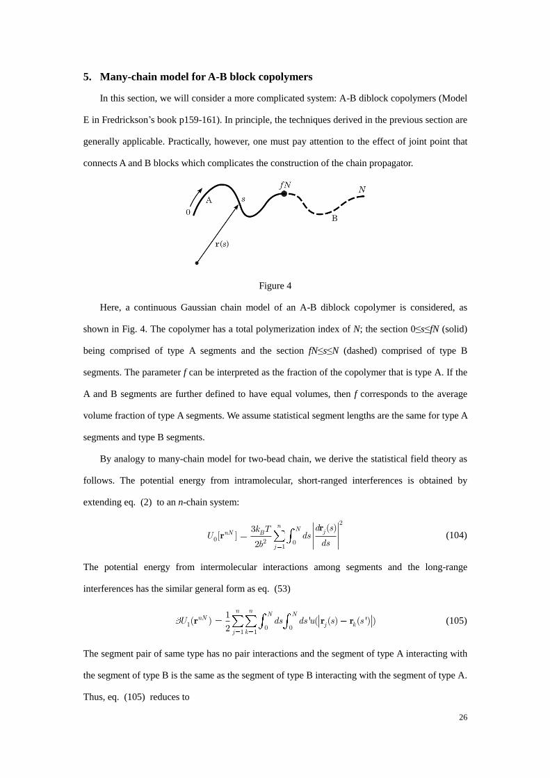
Figure 4
Here, a continuous Gaussian chain model of an A-B diblock copolymer is considered, as
shown in Fig. 4. The copolymer has a total polymerization index of N; the section 0≤s≤fN (solid)
being comprised of type A segments and the section fN≤s≤N (dashed) comprised of type B
segments. The parameter f can be interpreted as the fraction of the copolymer that is type A. If the
A and B segments are further defined to have equal volumes, then f corresponds to the average
volume fraction of type A segments. We assume statistical segment lengths are the same for type A
segments and type B segments.
By analogy to many-chain model for two-bead chain, we derive the statistical field theory as
follows. The potential energy from intramolecular, short-ranged interferences is obtained by
extending eq. (2) to an n-chain system:
2
0 2 01
( )3[ ]
2
n N jnN B
j
d sk TU ds
dsb
rr (104)
The potential energy from intermolecular interactions among segments and the long-range
interferences has the similar general form as eq. (53)
1 0 01 1
1( ) ' ( ( ) ( ') )
2
n n N NnN
j kj k
U ds ds u s sr r r (105)
The segment pair of same type has no pair interactions and the segment of type A interacting with
the segment of type B is the same as the segment of type B interacting with the segment of type A.
Thus, eq. (105) reduces to
27
1 0 01 1
01 1
01 1
1 1
1( ) ' ( ( ) ( ') )
2
1' ( ( ) ( ') )
2
1' ( ( ) ( ') )
2
1' ( ( ) ( ') )
2
n n fN fNnN
AA j kj kn n fN N
AB j kfNj kn n N fN
AB j kfNj kn n N N
BB j kfN fNj k
U ds ds u s s
ds ds u s s
ds ds u s s
ds ds u s s
r r r
r r
r r
r r
(106)
where uA,B denotes the pair interaction energy between segment of type A and segment of type B.
With the definition of microscopic density operators
0
1
( ) [ ( )]n fN
A jj
ds sr r r (107)
1
( ) [ ( )]n N
B jfNj
ds sr r r (108)
eq. (106) can be expresses as
11
( ) ' ( ) ( ' ) ( ')21
' ( ) ( ' ) ( ')21
' ( ) ( ' ) ( ')21
' ( ) ( ' ) ( ')2
nNA AA B
B BB B
A AB B
B AB A
U d d u
d d u
d d u
d d u
r r r r r r r
r r r r r r
r r r r r r
r r r r r r
(109)
It can be seen from
01
01
,01
01
' ( ) ( ' ) ( ')
' [ ( )] ( ' ) ( ')
' ( ') ( ' ) [ ( )]
' ( ') ( ( ) ' )
' ' [ ' ( ')] ( ( )
A AB B
n fN
j AB Bj
n fN
B AB jjn fN
B AB jj
nfN N
k AB jfNk
d d u
d d ds s u
ds d d u s
ds d u s
ds d ds s u s
r r r r r r
r r r r r r r
r r r r r r r
r r r r
r r r r1
01 1
01 1
' )
' ' ( ( ) ' ) [ ' ( ')]
' ( ( ) ( ') )
n
jn nfN N
AB j kfNj kn n fN N
AB j kfNj k
ds ds d u s s
ds ds u s s
r
r r r r r
r r
(110)
If we further introduce the Flory-type pair interaction energy
28
( ' ) ( ')AA AAu ur r r r (111)
( ' ) ( ')AB ABu ur r r r (112)
( ' ) ( ')AB ABu ur r r r (113)
Following the same procedure of eq (60), we have
2 21( ) ( ) ( ) ( ) ( )
2 2nN AA BB
A B AB A B
u uU d d u dr r r r r r r r (114)
By applying the incompressible condition 0 ( ) ( )A Br r , the first integral can be evaluated
as
2
2 2 2
2 2 20
20
20
( )
1 1 1( ) ( ) ( ) ( ) ( ) ( )
2 2 21 1
( ) ( ) ( ) ( )2 21 1
( ) ( ) ( ) ( ) ( ) ( )2 21
( ) ( )2
A
A B B A B A
A B A B
A B A B A B
A B
d
d
d
d
d
r r
r r r r r r r
r r r r r
r r r r r r r
r r r 0
20 0 0
20 0 0
20 0
01
0
1
1( ) ( )
21
( ) ( ) ( ) ( )2
( ) ( ) ( ) ( )2 2 2
[ ( )]2 2
[ ( )] ( ) ( )2
A B
A B A B
A B A B
n fN
jj
n N
j A BfNj
d d
d d d d
Vd ds s
d ds s d
nN
r r
r r r r r r
r r r r r r r r
r r r
r r r r r r
0 0 0
0
( )( ) ( )
2 2 2( ) ( )
A B
A B
nfN n N fNd
fnN d
r r r
r r r (115)
Similarly, the other integral can be evaluated to be
20( ) (1 ) ( ) ( )A A Bd f nN dr r r r r (116)
Substituting eq (115) and (116) into eq (114), we have
29
1
0
0
0
0 0
( )
( ) ( )2
(1 ) ( ) ( )2
( ) ( )
2 (1 )( ) ( )
2 2(1 )
( ) ( )2
nN
AAA B
BBA B
AB A B
AB AA BB AA BBA B
AA BBA B
U
ufnN d
uf nN d
u d
u u u fu f ud nN
fu f uv d nN
r
r r r
r r r
r r r
r r r
r r r
(117)
The Flory-Huggins interaction parameter is again given by
0
2
2AB AA BBu u u
v (118)
and the constant term is ignored to give the final form of Flory-type energy
1 0( ) ( ) ( )nNA BU v dr r r r (119)
The canonical partition function of diblock copolymers is again similar to that of two-bead chain
system
0 1 03
1exp ( ) ( ) ( ) ( )
!( )nN nN nN
A BnNT
Z d U Un
r r r r r (120)
Inserting eq. (104) and (119) into above equation, we have
2
0 03 2 01
( )31exp ( ) ( ) ( ) ( )
!( ) 2
n N jnN BA B A BnN
jT
d sk TZ d ds v d
dsn b
rr r r r r r
(121)
Using the delta functionals, it changes to
2
03 2 01
( )31exp ( ) ( )
!( ) 2
1 ( ) ( ) [ ( ) ( )] [ ( ) ( )]
n N jnN BA B A BnN
jT
A B A A B B
d sk TZ d ds v d
dsn b
rr r r r
r r r r r r
(122)
The delta functionals are then replaced by their complex exponential representations
30
2
03 2 01
23 2
( )31exp ( ) ( )
!( ) 2
exp ( )[1 ( ) ( )]
exp ( )[ ( ) ( )]
exp ( )[ ( ) ( )]
1exp
!( )
n N jnN BA B A BnN
jT
A B
A A A A
B B B B
nA Bn
T
d sk TZ d ds v d
dsn b
i d
w i d w
w i d w
dn
rr r r r
r r r r
r r r r
r r r r
r
2
02 01
0
( )3( ) ( )
2
exp ( ) ( ) ( ) ( ) ( )[ ( ) ( )]
exp ( ) ( ) ( ) ( )
n N jBA B
j
A B A A B B A B
A A B B
d sk Tds v d
dsb
w w i d w w
i d w w
rr r r
r r r r r r r r
r r r r r
(123)
The last line of above function can be evaluated the same as eq. (72), which leads to
0
1 1
01 1
01
( ) ( ) ( ) ( )
( ) ( ) ( ) ( )
( ) [ ( )] ( ) [ ( )]
( ) [ ( )] ( ) [ ( )]
( ( ))
A A B B
A A B B
n nfN N
A j B jfNj j
n nfN N
A j B jfNj jn fN
A jj
d w w
d w d w
d w ds s d w ds s
ds d w s ds d w s
dsw s
r r r r r
r r r r r r
r r r r r r r r
r r r r r r r r
r1
( ( ))n N
B jfNj
dsw sr
(124)
Substitute above equation into eq. (123), we have
3
0 0
2
22 0 0
1 1
1
!( )
exp ( ) ( ) ( ) ( ) ( )[ ( ) ( )] ( ) ( )
( )3exp ( ( )) ( ( ))
2
A B A BnNT
A A B B A B A B
n n N fN Njn BA j B jfN
j j
Z w wn
d iw iw i v
d sk Td ds i dsw s i dsw s
dsb
r r r r r r r r r r
rr r r
(125)
The last line of above equation is evaluated as
31
2
2 0 01
21
1 1 1 12 0 0
2 2
( )3exp ( ( )) ( ( ))
2
3 ( )exp ( ( )) ( ( ))
2
ex
n N fN NjnN BA j B jfN
j
N fN NfN N fN BA B A BfN
fN N fNA B
d sk Td ds i dsw s i dsw s
dsb
k T d sd d ds i dsw s i dsw s
dsb
d d
rr r r
rr r r r
r r2
22 22 0 0
2
2 0 0
2
2 0
3 ( )p ( ( )) ( ( ))
2
3 ( )exp ( ( )) ( ( ))
2
3 ( )exp ( (
2
N fN NB
A BfN
N fN NfN N fN B nAn Bn A n B nfN
NfN N fN BA B A
k T d sds i dsw s i dsw s
dsb
k T d sd d ds i dsw s i dsw s
dsb
k T d sd d ds i dsw s
dsb
rr r
rr r r r
rr r r
0
2
2 0 00
)) ( ( ))
3 ( )( )exp ( ( )) ( ( ))
2
nfN N
BfN
nN N fN N
BA BfN
t
i dsw s
k T d sd t ds i dsw s i dsw s
dsb
r
rr r r
(126)
The integral in the last line of above equation is just the single-chain partition function
2
2 0 00
3 ( )( )exp ( ( )) ( ( ))
2
N N fN NB
s A BfNt
k T d sZ d t ds i dsw s i dsw s
dsb
rr r r (127)
The first term in the exponential is just the internal energy of a continuous Gaussian chain, the
second term describes the interaction between A block and the corresponding external field which
is generated internally, and the third term describes the interaction between B block and the
corresponding external field.
The chain propagator is defined similarly to eq. (35). However, it has two forms depending on
the value of s. For 0≤s≤fN, it is defined as
32
2
2 20 00
( ')3 3( , ) ( )exp ' ' [ ( ')] ( )
'2 2
sN s s s
At
d sq s d t ds ds iw s s
dsb s b
rr r r r r
(128)
Retracing the steps from eq. (36) to eq. (40), we can obtain the Fokker-Planck equation
2
2( , ) ( , ) ( ) ( , )6 Ab
q s q s iw q ssr r r r (129)
Similarly, for fN≤s≤N, the chain propagator is defined as
3
2
20
2
20 0
3( , ) ( )
2
( ')3exp ' ' [ ( ')] ' [ ( ')] ( )
'2
sN s
t
s fN s
A AfN
q s d tb s
d sds ds iw s ds iw s s
dsb
r r
rr r r r
(130)
and the resulted Fokker-Planck equation is given by
32
2
2( , ) ( , ) ( ) ( , )6 Bb
q s q s iw q ssr r r r (131)
The initial condition is
( ,0) 1q r (132)
The normalized single-chain partition function is obtained by following the steps from eq. (43) to
eq. (46)
1
[ , ] ( , ) ( , )A BQ iw iw d q s q N sV
r r r (133)
In particular, for s=0, Q is evaluated to be
1
[ , ] ( , )A BQ iw iw d q NV
r r (134)
With the definition of Q, we now reach the final result of the statistical field theory for diblock
copolymer melts:
0 exp( )A B A BZ Z w w H (135)
where the effective Hamiltonian is
0 0( ) ( ) ( ) ( ) ( ) ( ) ( )[ ( ) ( )] ln [ , ]A B A A B B A B A BH d v iw iw i n Q iw iwr r r r r r r r r r
(136)
and the explicit form of the prefactor Z0 is unimportant.
The single-chain partition function describes a single chain in an external field. In light of
section 3, we can define two single-chain density operators:
1
0( ) [ ( )]
fN
A ds sr r r (137)
1 ( ) [ ( )]N
B fNds sr r r (138)
Invoking the universal relation (eq. (88)) between the average segment density and the average
single-chain segment density established in section 4, we have
1( ) ( )A Anr r (139)
1( ) ( )B Bnr r (140)
Therefore, we only need to calculate the average single-chain segment densities.
Since the external field exerting on A block is different from that exerting on B block, as can
be seen in the single-chain partition function (eq. (127)), it is impossible to calculate the average
33
single-chain segment densities from only q propagator. Taking 1 ( )A r as an example, we see
that
1
21
2 0 00
00
2
2 0 0
( )
3 ( )1( ) ( )exp ( ( )) ( ( ))
2
1( ) [ ( )]
3 ( ')exp ' ' ( ( ')) ( ( '))
'2
1
A
N N fN NB
A A BfNt
N fN
t
N fN NB
A BfN
k T d sd t ds i dsw s i dsw s
Z dsb
d t ds sZ
k T d sds i ds w s i dsw s
dsb
dsZ
r
rr r r r
r r r
rr r
00
2
2 0 0
00
2
2 0 0
( )
3 ( ')exp ' ' ( ( ')) ' ( ( ')) [ ( )]
'2
1( ) ( ) [ ( )]
3 ( ')exp ' ' ( ( ')) ' ( ( '))
'2
NfN
t
N fN NB
A BfN
NfN
t
N fN NB
A BfN
d t
k T d sds i ds w s i ds w s s
dsb
ds d t d s sZ
k T d sds i ds w s i ds w s
dsb
r
rr r r r
r r r r
rr r
32 2
0
32
2
2 2 0 00
3( )
2
2 2
[ ( )]
1 2
3
3 ( ')3( )exp ' ( ( ')) [ ( )]
'2 2
3 ( ')3( )exp '
2 2
N
s
N s
NfN
N s s sB
At
N N NB
t s
s
b sds
Z
k T d sd t ds i dsw s s
dsb s b
k T d sd t ds
b s b
r r
rr r r r
rr
2
0
03
2( )2
2 2
' ( ( ')) ' ( ( ')) [ ( )]'
( , )
3 ( ')3( )exp ' ( ( ')) ' ( ( ')) [ ( )]
'2 2
N s
N fN N
A Bs s fN
fN
N N N N fN NB
A Bs s fNt s
i ds w s i ds w s sds
Zdsq s
ZV
k T d sd t ds i ds w s i ds w s s
dsb s b
r r r r
r
rr r r r r
(141)
The last line of above equation is neither q(r, s) nor q(r, N-s). However, we can rewrite it to
3( )
2
20
2(1 )
2 0 0 (1 )
3( )
2
3 ( ')exp ' ' ( ( ')) ' ( ( ')) [ ( )]
'2
N sN N N s
t
N s f N N sB
B AfN
d tb s
k T d sds ds iw s ds iw s N s
dsb
r
rr r r r
(142)
This expression says it has the same structure of the chain propagator q, but instead of starting
34
propagation from the end of block A, it starts at the end of block B. Note that the range of N-s in
the eq. (142) is (1-f)N≤s≤N. So we can define a complementary chain propagator q* when s is in
the range of (1-f)N≤s≤N:
3
2*2
02
(1 )
2 0 0 (1 )
3( , ) ( )
2
3 ( ')exp ' ' ( ( ')) ' ( ( ')) [ ( )]
'2
sN s
t
s f N sB
B AfN
q s d tb s
k T d sds ds iw s ds iw s s
dsb
r r
rr r r r
(143)
This q* also satisfies a Fokker-Planck equation (for (1-f)N≤s≤N)
2
* 2 * *( , ) ( , ) ( ) ( , )6 Ab
q s q s iw q ssr r r r (144)
Using the definition q* and invoking the definition of Q, eq. (141) becomes
1 *
0
1( ) ( , ) ( , )
[ ( ), ( )]
fN
AA B
dsq s q N sVQ iw iw
r r rr r
(145)
The derivation of the above equation for the segment of type B is similar. By retracing the
steps from eq. (141) to eq. (145), we can obtain the average single-chain segment density
1 *1( ) ( , ) ( , )
[ ( ), ( )]
N
B fNA B
dsq s q N sVQ iw iw
r r rr r
(146)
In the above, the range for N-s is 0≤s≤(1-f)N, and the form of the complementary chain propagator
q* defined in this range is
32
2*2 2 0 0
0
3 ( ')3( , ) ( )exp ' ' ( ( ')) [ ( )]
'2 2
sN s s sB
Bt
k T d sq s d t ds ds iw s s
dsb s b
rr r r r r
(147)
And it satisfies the following Fokker-Planck equation (for 0≤s≤(1-f)N)
2
* 2 * *( , ) ( , ) ( ) ( , )6 Bb
q s q s iw q ssr r r r (148)
As long as we find the tools for calculating the ensemble average densities for A and B beads,
we are ready to derive the self-consistent field theory. The self-consistent field theory is obtained
by imposing the mean-field approximation to the statistical field theory. The mean-field SCF
equations are obtained by the saddle-approximation which has the same expressions as in eq.
(101), eq. (102), and eq. (103), but with ensemble average densities according to this section.
35
6. Many-chain model for solutions of A-B diblock copolyelectrolytes
In this section, we will extend the many-chain model for diblock copolymer melts to charged
systems. In particular, we will consider A-B diblock copolyelectrolytes in a solution of
small-molecules, usually water, with presence of salt. We treat the solvent explicitly, which
interacts with polymer segments with a Flory-type interaction. The chains are again taken to be
continuous Gaussian chains and the charge distribution can be either smeared (corresponding to
strongly dissociating polyelectrolytes, e.g. PAA) and annealed (corresponding to weakly
dissociating polyelectrolytes, e.g. polyethylene-poly(acrylic acid) statistical copolymer). We also
assume that the counterions dissociated from polyelectrolytes are identical to the ions form salt
that carry the same type of charge, and denote cations by + and anions by -. Integer variables v+>0,
v- < 0, and vP are used to denote the valencies of cations, anions and the ions bounded to P (=A, B)
polymer segments, respectively.
In this model, besides the potential energy for the continuous Gaussian chain and the potential
energy from the intermolecular interactions among polymer segments and solvent molecules, there
is an additional energetic contribution arisen from the long-ranged Coulomb interactions. The
Coulomb interaction is the most distinctive feature for charged systems. The Coulomb potential
acting between an ion with charge eZj and a second ion with charge eZk, separated by a distance r
in a uniform dielectric medium, can be written
2
( ) j ke
e Z Zu r
r (149)
where cgs units are employed and is the dielectric constant. The Coulomb potential is often
rewritten in the form
( ) B j ke B
l Z Zu r k T
r (150)
where
2
BB
el
k T (151)
is the so-called Bjerrum length. It defines a length scale at which the electrostatic interaction is
comparable to the thermal energy kBT.
The electrostatic interaction energy can be obtained by summing the electric potential of all
36
pairs of charged species across the whole system, which also has the similar general form of eq.
(53)
0 01 1
01 1
01 1
1 1
1 1
1 1
1[ ] ' ( ( ) ( ') )
2
( ( ) )
( ( ) )
1( )
2
( )
1( )
2
n n N NnN n ne e j k
j knn N
e j kj k
nn N
e j kj kn n
e j kj k
n n
e j kj kn n
e j kj k
U ds ds u s s
dsu s
dsu s
u
u
u
r r r
r r
r r
r r
r r
r r
(152)
where n, n+ and n- are the number of diblock copolymers, cations and anions, respectively. The
first to the sixth lines of eq. (152) represent the Coulomb interactions between polymer segments,
between polymer segments and cations, between polymer segments and anions, between cations,
between cations and anions, and between anions, respectively. The singular interactions of each
ion with itself included in eq. (152) only lead to a shift in chemical potential of each species that
has no thermodynamic consequence. To write eq. (152) in a compact form, it is helpful to define a
microscopic charge density
1
( ) ( )n
jj
r r r (153)
1
( ) ( )n
jj
r r r (154)
01 1
( ) ( ( )) ( ( ))
( ) ( )
n nfN N
e A A j B B jfNj j
v ds s v ds s
v v
r r r r r
r r
(155)
where A and B are the degree of ionization for block A and block B, respectively. In writing eq.
(155), we have assumed the smeared charge distribution. The charge density operator ( )e r is in
units of e. The system satisfies the electroneutrality condition, thus
37
01
1
1
1
01
1
1
1
( ) ( ( ))
( ( ))
( )
( )
( ( ))
( ( ))
( )
( )
n fN
e A A jjn N
B B jfNj
n
jjn
jjn fN
A A jjn N
B B jfNj
n
jjn
jj
d d v ds s
d v ds s
d v
d v
v ds d s
v ds d s
v d
v d
r r r r r
r r r
r r r
r r r
r r r
r r r
r r r
r r r
01 1 1 1
1 1
(1 )
0
n nn nfN N
A A B B fNj j j j
A A B B
v ds v ds v v
v nfN v n f N v n v n (156)
So we have the relation between the numbers of different species:
(1 ) 0A A B Bv nfN v n f N v n v n (157)
The electrostatic interaction energy can thus be written
1
[ ] ' ( ) ( ')2 '
nN n n Be e e
lU d dr r r r r
r r (158)
This equality can be verified as follows
38
01 1
01 1
1' ( ) ( ')
2 '
1' ( ( )) ( ( )) ( ) ( )
2
( ' ( )) ( ' ( )) ( ') ( ')'
Be e
n nfN N
A A j B B jfNj j
n nfN NB
A A j B B jfNj j
ld d
d d v ds s v ds s v v
lv ds s v ds s v v
r r r rr r
r r r r r r r r
r r r r r rr r
0 01 1
01 1
1' ( ( )) ( ' ( ))
2 '
1' ( ( )) ( ' ( ))
2 '
1' (
2
n nfN fNB
A A j A A jj jn nfN N
BA A j B B jfN
j j
A A j
ld d v ds s v ds s
ld d v ds s v ds s
d d v ds
r r r r r rr r
r r r r r rr r
r r r r0
1
01
01 1
( )) ( ')'
1' ( ( )) ( ')
2 '
1' ( ( )) ( ' ( ))
2 '
1
2
n fNB
jn fN
BA A j
jn nN fN
BB B j A A jfN
j j
ls v
ld d v ds s v
ld d v ds s v ds s
d
rr r
r r r r rr r
r r r r r rr r
r1 1
1
1
' ( ( )) ( ' ( ))'
1' ( ( )) ( ')
2 '
1' ( ( ))
2 '
n nN NB
B B j B B jfN fNj jn N
BB B jfN
jn N
BB B jfN
j
ld v ds s v ds s
ld d v ds s v
ld d v ds s v
r r r r rr r
r r r r rr r
r r r rr r
01
1
( ')
1' ( ) ( ' ( ))
2 '
1' ( ) ( ' ( ))
2 '
1' ( ) ( ')
2 '
1' ( )
2
n fNB
A A jjn N
BB B jfN
j
B
ld d v v ds s
ld d v v ds s
ld d v v
d d v
r
r r r r rr r
r r r r rr r
r r r rr r
r r r
01
1
( ')'
1' ( ) ( ' ( ))
2 '
1' ( ) ( ' ( ))
2 '
1' ( ) ( ')
2 '
1'
2
B
n fNB
A A jjn N
BB B jfN
j
B
lv
ld d v v ds s
ld d v v ds s
ld d v v
d d v
rr r
r r r r rr r
r r r r rr r
r r r rr r
r r ( ) ( ')'
Bl vr rr r
(159)
The sum of 1st, 2
nd, 3
rd and 4
th terms after the second equal sign in eq. (159) corresponds to the
first term of the right-hand side of eq. (152). Similarly, the sum of 3rd
, 7th
, 9th
, and 10th terms, 4
th,
8th, 13
th, and 14
th terms, 11
th terms, the sum of 12
th and 15
th terms, and 16
th terms after the second
39
equal sign in eq. (159) correspond to the 2nd
, 3rd
, 4th
, 5th
, and 6th of the right-hand side of eq. (152),
respectively.
The potential energy from unperturbed continuous Gaussian chains is still given by (the same
as eq. (104))
2
0 2 01
( )3[ ]
2
n N jnN
j
d sU ds
dsb
rr (160)
The short-range (e.g. van der Waals) interaction energy of the system is approximated by the
energy arisen from Flory-type interactions. Following the treatment analogous in section 5, we can
express the short-range interaction energy as
1 0 0 0( ) ( ) ( ) ( ) ( ) ( ) ( )SnN nAB A B AS A S BS B SU v d v d v dr r r r r r r r r r (161)
where AB is the Flory-Huggins interaction parameter between polymer segments of type A and
type B, AS is that between the polymer segments of type A and the solvent molecules, and
BS is that between the polymer segments of type A and the solvent molecules. In the above
equation, there are two additional terms describing the Flory-type interactions between polymer
segments and solvent molecules compared to eq. (114). In eq. (161), the volumes of the statistical
segment (either of type A or B) and the solvent molecule are assumed to be identical. The
microscopic segment density and microscopic solvent density are defined to be
0
1
( ) [ ( )]n fN
A jj
ds sr r r (162)
1
( ) [ ( )]n N
B jfNj
ds sr r r (163)
1
( ) [ ]Sn
S jj
r r r (164)
Combining the potential energies in eq. (158), (160) and (161), we can write the canonical
partition function as
0 13
0
1exp ( ) ( ) ( )
! ! ! !( )
( ) ( ) ( ) ( ( ))
S S
S
nN n n n nN n nnN nnNenN n n n
S T
A B S e
Z d U U Un n n n
d
r r r r
r r r r r
40
(165)
The next task is to perform a particle-to-field transformation to the above partition function.
To present here more clearly, we will do the transformation separately. Since it is not necessary to
do transformation on U0, we first do the transformation for U1. Upon using the identity involving a
delta functional (eq. (50)), we have
1 0
0 0 0
0
exp ( ) [ ( ) ( ) ( )]
exp ( ) ( ) ( ) ( ) ( ) ( )
[ ( ) ( )] [ ( ) ( )] [ ( ) ( )] [ ( ) ( ) ( )]
SnN nA B S
A B S
AB A B AS A S BS B S
A A B B S S A B S
U
v d v d v d
r r r r
r r r r r r r r r
r r r r r r r r r
(166)
And replacing the delta functionals with their complex exponential representations, it becomes
1 0
0 0 0
exp ( ) [ ( ) ( )]
exp ( ) ( ) ( ) ( ) ( ) ( )
exp ( )( ( ) ( ))
exp ( )( ( ) ( ))
exp
SnN nA B
A B S
AB A B AS A S BS B S
A A A A
B B B B
S
U
v d v d v d
w i d w
w i d w
w i d
r r r
r r r r r r r r r
r r r r
r r r r
0
0 0 0
( )( ( ) ( ))
exp ( )( ( ) ( ) ( ))
exp ( ) ( ) ( ) ( ) ( ) ( )
exp ( ) ( ) ( ) ( ) ( ) (
S S S
S A B S
A B S A B S
AB A B AS A S BS B S
A A B B S S
w
i d w
w w w
v d v d v d
i d w w w
r r r r
r r r r r
r r r r r r r r r
r r r r r r 0) ( )( ( ) ( ) ( ))
exp ( ) ( ) ( ) ( ) ( ) ( )
S A B S
A A B B S S
w
i d w w w
r r r r r
r r r r r r r
(167)
The exponential term with Ue can be treated similarly. Upon using the identity involving the
delta functional (eq. (50)), we have
exp ( ) ( ( ))
1exp ' ( ) ( ') ( ) ( ) ( ( ))
2 '
nN n ne e
Be e e e e e
U d
ld d d
r r r
r r r r r r r rr r
(168)
Substituting the complex exponential form of the delta functional into above equation leads to
41
exp ( ) ( ( ))
1exp ' ( ) ( ') exp ( )( ( ) ( )) exp ( )
2 '
1exp ( ) exp ' ( ) ( ') (
2 '
nN n ne e
Be e e e e e
Be e e e
U d
ld d i d d i d
ld i d d d i d
r r r
r r r r r r r r r rr r
r r r r r r rr r
) ( ) exp ( ) ( )
1exp ( ) ( ) exp ' ( ) ( ') ( ( ) ) ( )
2 '
e e
Be e e e e
i d
ld i d d d i d
r r r r r
r r r r r r r r r rr r
(169)
Fortunately, the functional inside the curly bracket is a typical Gaussian functional which can be
evaluated analytically. One of Gaussian integral formulas is (see Fredrickson’s book p398-399)
10
1 1exp ' ( ) ( , ') ( ') ( ) ( ) exp ' ( ) ( , ') ( ')
2 2f dx dx f x A x x f x i dxJ x f x C dx dx J x A x x J x
(170)
where A(x,x’) is assumed to be real, symmetric, and positive definite. The functional inverse of A,
A-1
, is defined by
1' ( , ') ( ', '') ( '')dx A x x A x x x x (171)
and the constant C0 is
01
exp ' ( ) ( , ') ( ')2
C f dx dx f x A x x f x (172)
In our case here, A is
'
BlAr r
(173)
its functional inverse is
1 21( ')
4 B
Al
r r (174)
and J is
( )J r (175)
It follows that
42
20
20
0
1exp ' ( ) ( ') ( ( ) ) ( )
2 '
1 1exp '( ( ) ) ( ') ( ( ') )
2 4
1exp ( ( ) ) ' ( ')( ( ') )
8
1exp ( ( )
8
Be e e e
B
B
B
ld d i d
C d dl
C d dl
C dl
r r r r r r rr r
r r r r r r
r r r r r r
r r 2
20
20
) ' ( ')( ( ') )
1exp ( ( ) ) ( ( ) )
8
1exp ( ( ) ) ( )
8
B
B
d
C dl
C dl
r r r r
r r r
r r r
(176)
The integral in the above equation can be evaluated by integrating by part
2
2
2
( ( ) ) ( )
( ) [ ( )] ( )
( ) ( ) ( ) ( ) ( )
( ) ( )
( ) ( )
( )
d
d d
d
d
d
d
r r r
r r r r
r r r r r
r r
r r r
r r
(177)
Inserting eq. (177) into eq. (176), we have
2
01 1
exp ' ( ) ( ') ( ) ( ) exp ( )2 ' 8
Be e e e
B
ld d i d C d
lr r r r r r r r r
r r
(178)
Then the above equation is substituted into eq. (169), which leads to the final field form for
electrostatic interaction energy
20
20
1exp ( ) exp ( ) ( ) exp ( )
8
1exp ( ) ( ) ( )
8
nN n ne e
B
eB
U d C i d dl
D d il
r r r r r r
r r r r
(179)
where the integration result with respect to is absorbed into D0. In literature, an effective
Hamiltonian for electrostatic interaction energy is often used, which is just the integral inside the
square bracket in the second line of eq. (179):
21
[ ] ( ) ( ) ( )8e eB
H d il
r r r r (180)
43
Note that the real electric potential field is usually replaced by a pure imaginary variable in
literature. In this convention, the Hamiltonian is expressed as
21
[ ] ( ) ( ) ( )8e eB
H dl
r r r r (181)
The negative sign is coming from the square of imaginary number i:
2
22
2
2
1[ ] ( ) ( ) ( 1) ( )
8
1( ) ( ) ( )
8
1( ) ( ) ( )
8
1( ) ( ) ( )
8
e eB
eB
eB
eB
H d il
d i il
d i il
dl
r r r r
r r r r
r r r r
r r r r
(182)
It is now ready for us to finish the particle-to-field transformation. Substituting eq. (167),
(179), the partition function is given by
3
2
2 01
0 0 0
1
! ! ! !( )
( )3exp
2
exp ( ) ( ) ( ) ( ) ( ) ( )
exp ( ) ( ) ( ) ( )
S
S
nN n n n
nN n n nS T
n N j
j
A B S A B S
AB A B AS A S BS B S
A A B B
Z dn n n n
d sds
dsb
w w w
v d v d v d
i d w w
r
r
r r r r r r r r r
r r r r r 0
20
( ) ( ) ( )( ( ) ( ) ( ))
exp ( ) ( ) ( ) ( ) ( ) ( )
1exp ( ) ( ) ( )
8
S S S A B S
A A B B S S
eB
w w
i d w w w
D d il
r r r r r r
r r r r r r r
r r r r
(183)
Rearranging the above equation in terms of rnN+n
S+n
++n
- dependent and independent part, we have
44
0
3
0 0 0
0
! ! ! !( )
exp ( ) ( ) ( ) ( ) ( ) ( )
exp ( ) ( ) ( ) ( ) ( ) ( ) ( )( ( ) ( ) ( ))
exp
SnN n n nS T
A B S A B S
AB A B AS A S BS B S
A A B B S S A B S
DZ
n n n n
w w w
v d v d v d
i d w w w
r r r r r r r r r
r r r r r r r r r r r
2
2
2 01
1( )
8
( )3exp ( ) ( ) ( ) ( ) ( ) ( ) ( ) ( )
2
S
BnN n n n
n N jA A B B S S e
j
dl
d
d sds i d w w w i d
dsb
r r
r
rr r r r r r r r r r
(184)
The last two lines of the above equation can be evaluated by substituting back the definition of all
microscopic density operators
45
2
2 01
2
2 01
01
( )3exp ( ) ( ) ( ) ( ) ( ) ( ) ( ) ( )
2
( )3exp
2
exp ( ) [ ( )]
S
S
nN n n n
n N jA A B B S S e
j
n N jnN n n n
j
n fN
A jj
d
d sds i d w w w i d
dsb
d sd ds
dsb
i d w ds s
r
rr r r r r r r r r r
rr
r r r r1 1
01 1
1 1
( ) [ ( )] ( ) [ ]
( ( )) ( ( ))
exp ( )
( ) ( )
Snn N
B j S jfNj j
n nfN N
A A j B B jfNj jn n
j jj j
w ds s w
v ds s v ds s
i d
v v
r r r r r r
r r r r
r r
r r r r
2
2 0
01
( )3
2
exp ( ) ( ) [ ( )]
( ) ( ) [ ( )]
exp
S
N j
n fNnN n n nA A A j
j N
B B B jfN
d sds
dsb
d i ds d w v s
i ds d w v s
i
r
r r r r r r
r r r r r
1
1
12
2 0 0
( ) [ ]
exp ( ) ( )
exp ( ) ( )
( )3( ) ( ) [ ( )]
2exp
( ) ( ) [ (
Sn
S jjn
jj
n
jj
N fNjA A A jnN
N
B B B jfN
d w
i d v
i d v
d sds i d w v ds s
dsbd
i d w v ds s
r r r r
r r r r
r r r r
rr r r r r
r
r r r r r1
1 1 1
2
2 0
0
)]
exp ( ) exp ( ) exp ( )
( )3
2
( )exp [ ( )] [ ( )]
[ ( )] [ ( )]
S
n
j
nn n
j S j j j j jj j j
N
fN
A A A
N
B B BfN
d iw d iv d iv
d sdsdsb
d t i ds w s v s
i ds w s v s
r r r r r r
r
r r r
r r1
exp ( )
exp ( )
exp ( )
S
n
N
t
n
S
n
n
d iw
d iv
d iv
r r
r r
r r
(185)
The three integrals in the last three lines of above equations can be interpreted as single-particle
46
partition functions for the solvent molecule, the cations, and the anions, respectively. Thus, we
have
exp ( )S SZ d iwr r (186)
exp ( )Z d v ir r (187)
exp ( )Z d v ir r (188)
We then define the normalized partition functions as in section 5 accordingly,
0
exp ( ) 1exp ( )
1
SSS S
S
d iwZQ d iw
Z Vd
r rr r
r (189)
0
exp ( ) 1exp ( )
1
d v iZQ d v i
Z Vd
r rr r
r (190)
0
exp ( ) 1exp ( )
1
d v iZQ d v
Z Vd
r rr r
r (191)
The ensemble average particle density for these three species can be calculated as
1
1
( ) ( )
( )
' ( )exp ( ')
' exp ( ')
' [ ']exp ( ')
' exp ( ')
exp ( )
S S
S S
S S
S
S
S
S
S
SS
S
n
d iwn
d iw
d iwn
d iw
niw
VQ
r r
r
r r r
r r
r r r r
r r
r
(192)
1
1
( ) ( )
( )
' ( )exp ( ')
' exp ( ')
' [ ']exp ( ')
' exp ( ')
exp ( )
n
d v in
d v i
d v in
d v i
nv i
VQ
r r
r
r r r
r r
r r r r
r r
r
(193)
47
1
1
( ) ( )
( )
' ( )exp ( ')
' exp ( ')
' [ ']exp ( ')
' exp ( ')
exp ( )
n
d v in
d v i
d v in
d iv i
nv i
VQ
r r
r
r r r
r r
r r r r
r r
r
(194)
where the relation of eq. (88) has been used.
Now, let’s turn to the first term after the last equal sign of eq. (185). It should be looked
familiar though it is a rather complicated object at a first glance. In comparison with eq. (127), we
immediately find that the integral in the curly bracket of that term is just the single-chain partition
function for the charged diblock copolymer, which has the form
2
2 0
01
( )3
2
( )exp [ ( )] [ ( )]
[ ( )] [ ( )]
N
N fN
C A A At N
B B BfN
d sdsdsb
Z d t i ds w s v s
i ds w s v s
r
r r r
r r
(195)
The only different between the single-chain partition functions of the neutral diblock copolymer
and the charged diblock copolymer is the later has an additional field describing the electrostatic
interactions. Therefore, there is no need to go through the steps from eq. (128) to eq. (148) to
obtain expressions for calculating the normalized single-chain partition functions, chain
propagators, and the ensemble average density of type A segments and type B segments. Just
replacing wA by
A A Aw v (196)
and replacing wB by
B B Bw v (197)
Here, we only summarize the final results:
The statistical field theory for diblock copolyelectrolyte solutions is
exp( )A B S A B SZ w w w H (198)
where
48
0 0 0
0
2
[ ( ) ( ) ( ) ( ) ( ) ( )
( ) ( ) ( ) ( ) ( ) ( )
( )( ( ) ( ) ( ))
1( ) ]
8ln ln ln ln
AB A B AS A S BS B S
A A B B S S
A B S
B
C S S
H d v v v
iw iw iw
i
ln Q n Q n Q n Q
r r r r r r r
r r r r r r
r r r r
r
(199)
and the prefactor Z0 is unimportant.
The normalized single-chain partition function can be calculated by
1( , ) ( , )
1( , )
CQ d q s q N sV
d q NV
r r r
r r (200)
or equivalently by
* *
*
1( , ) ( , )
1( , )
CQ d q s q N sV
d q NV
r r r
r r (201)
where the propagator q is determined by the following modified diffusion functions
22
22
( , ) [ ( ) ( )] ( , ), if ( , ) 6
( , ) [ ( ) ( )] ( , ), if 6
A A A
B B B
bq s iw v i q s s fNq s
s bq s iw v i q s s fN
r r r rr
r r r r
(202)
and the complementary chain propagator q* is determined similarly by
22 * *
*2
2 * *
( , ) [ ( ) ( )] ( , ), if (1 )6( , )
( , ) [ ( ) ( )] ( , ), if (1 )6
B B B
A A A
bq s iw v i q s s fN
q ss b
q s iw v i q s s fN
r r r rr
r r r r
(203)
The ensemble average segment densities of A and B segments are constructed by composing
forward and backward propagators (propagator and complementary propagator), giving rise to the
expressions
*
0
1( ) ( , ) ( , )
fN
AC
dsq s q N sVQ
r r r (204)
*1( ) ( , ) ( , )
N
B fNC
dsq s q N sVQ
r r r (205)
Note that each field variable appearing in eq. (199), (202), and (203) is associated with the
imaginary number i. Thus we can absorb i into field variables which results in pure imaginary
fields. With these changes, eq. (199), (202), and (203) become
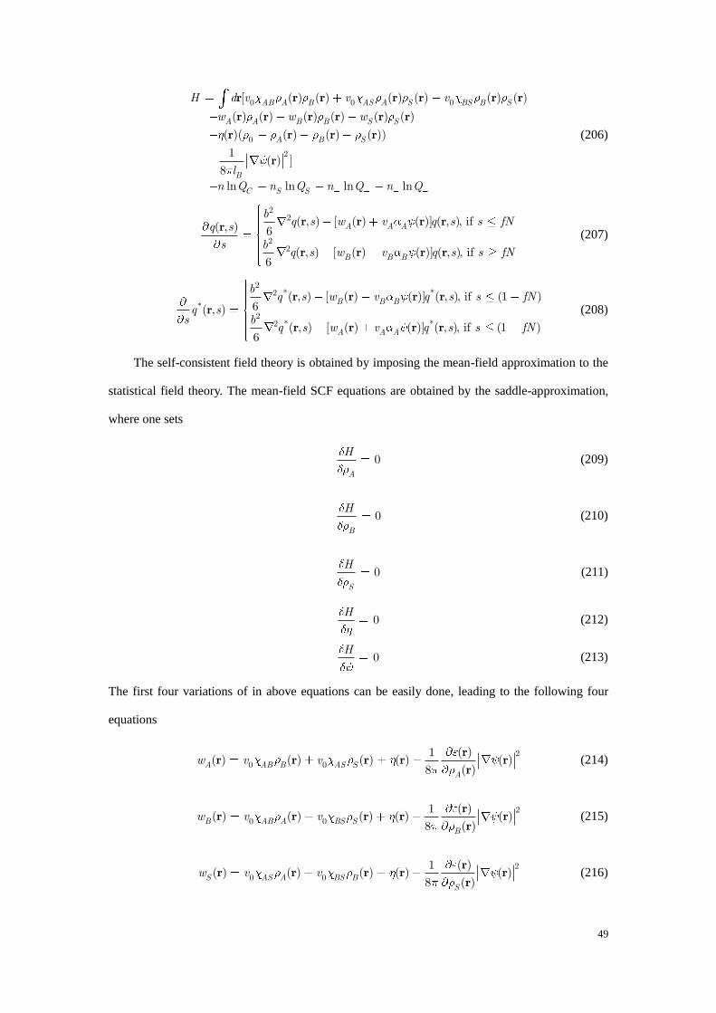
49
0 0 0
0
2
[ ( ) ( ) ( ) ( ) ( ) ( )
( ) ( ) ( ) ( ) ( ) ( )
( )( ( ) ( ) ( ))
1( ) ]
8ln ln ln ln
AB A B AS A S BS B S
A A B B S S
A B S
B
C S S
H d v v v
w w w
ln Q n Q n Q n Q
r r r r r r r
r r r r r r
r r r r
r
(206)
22
22
( , ) [ ( ) ( )] ( , ), if ( , ) 6
( , ) [ ( ) ( )] ( , ), if 6
A A A
B B B
bq s w v q s s fNq s
s bq s w v q s s fN
r r r rr
r r r r
(207)
22 * *
*2
2 * *
( , ) [ ( ) ( )] ( , ), if (1 )6( , )
( , ) [ ( ) ( )] ( , ), if (1 )6
B B B
A A A
bq s w v q s s fN
q ss b
q s w v q s s fN
r r r rr
r r r r
(208)
The self-consistent field theory is obtained by imposing the mean-field approximation to the
statistical field theory. The mean-field SCF equations are obtained by the saddle-approximation,
where one sets
0A
H (209)
0B
H (210)
0S
H (211)
0H
(212)
0H
(213)
The first four variations of in above equations can be easily done, leading to the following four
equations
2
0 0
( )1( ) ( ) ( ) ( ) ( )
8 ( )A AB B AS SA
w v vr
r r r r rr
(214)
2
0 0
( )1( ) ( ) ( ) ( ) ( )
8 ( )B AB A BS SB
w v vr
r r r r rr
(215)
2
0 0
( )1( ) ( ) ( ) ( ) ( )
8 ( )S AS A BS BS
w v vr
r r r r rr
(216)
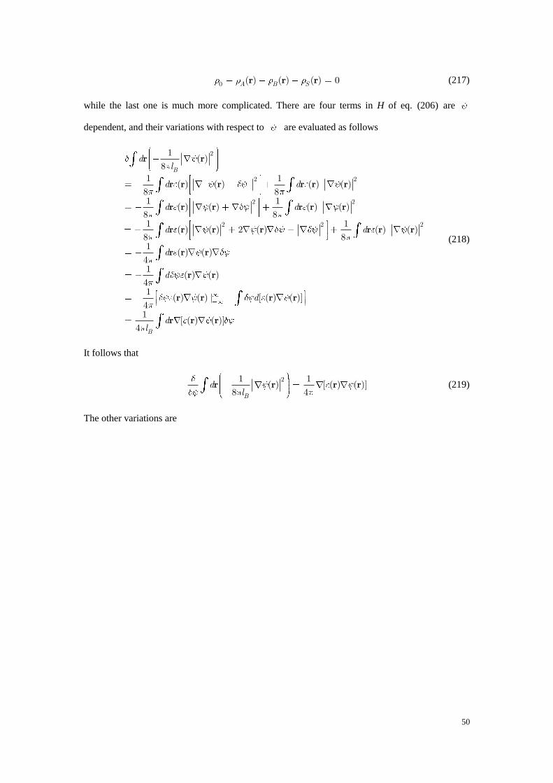
50
0 ( ) ( ) ( ) 0A B Sr r r (217)
while the last one is much more complicated. There are four terms in H of eq. (206) are
dependent, and their variations with respect to are evaluated as follows
2
2 2
2 2
2 2 2
1( )
81 1
( ) ( ) ( ) ( )8 81 1
( ) ( ) ( ) ( )8 81 1
( ) ( ) 2 ( ) ( ) ( )8 81
( ) ( )41
4
B
dl
d d
d d
d d
d
d
r r
r r r r r r
r r r r r r
r r r r r r r
r r r
( ) ( )
1( ) ( ) | [ ( ) ( )]
41
[ ( ) ( )]4 B
d
dl
r r
r r r r
r r r
(218)
It follows that
21 1
( ) [ ( ) ( )]8 4B
dl
r r r r (219)
The other variations are
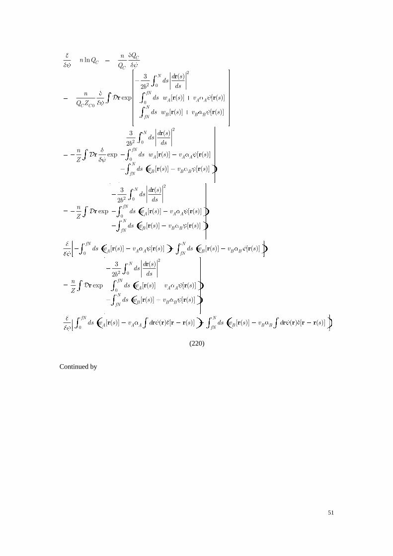
51
2
2 0
00
2
2 0
0
ln
( )3
2
exp [ ( )] [ ( )]
[ ( )] [ ( )]
( )3
2
exp [ ( )] [ ( )]
[ (
CC
C
N
fN
A A AC C N
B B BfN
N
fN
A A A
B
Qnn Q
Q
d sdsdsb
nds w s v s
Q Zds w s v s
d sdsdsb
nds w s v s
Zds w s
r
r r r
r r
r
r r r
r
2
2 0
0
)] [ ( )]
( )3
2
exp [ ( )] [ ( )]
[ ( )] [ ( )]
[ ( )] [ ( )] [ ( )] [ (
N
B BfN
N
fN
A A A
N
B B BfN
A A A B B B
v s
d sdsdsb
nds w s v s
Zds w s v s
ds w s v s ds w s v s
r
r
r r r
r r
r r r r0
2
2 0
0
0
)]
( )3
2
exp [ ( )] [ ( )]
[ ( )] [ ( )]
[ ( )] ( ) [ ( )] [ ( )] ( ) [ ( )]
fN N
fN
N
fN
A A A
N
B B BfN
fN N
A A A B B BfN
d sdsdsb
nds w s v s
Zds w s v s
ds w s v d s ds w s v d s
r
r r r
r r
r r r r r r r r r r
(220)
Continued by
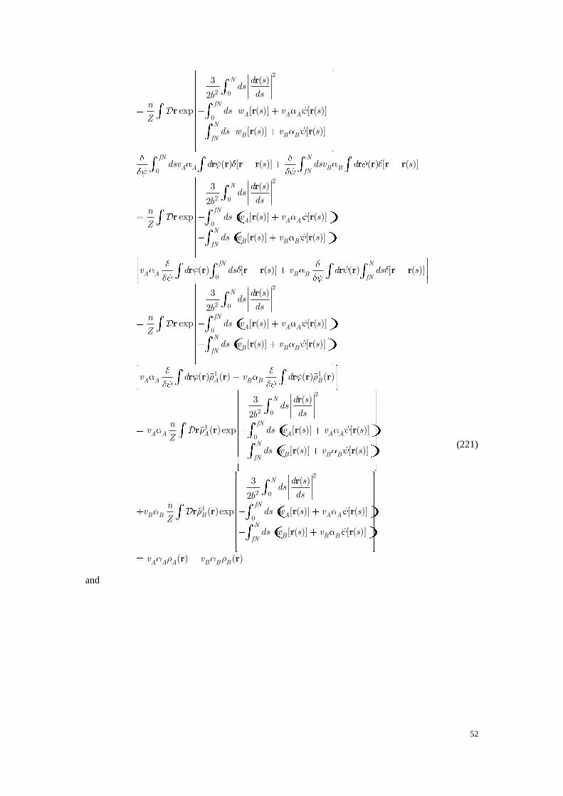
52
2
2 0
0
0
2
2 0
( )3
2
exp [ ( )] [ ( )]
[ ( )] [ ( )]
( ) [ ( )] ( ) [ ( )]
( )3
2
exp [ (
N
fN
A A A
N
B B BfN
fN N
A A B BfN
N
A
d sdsdsb
nds w s v s
Zds w s v s
dsv d s dsv d s
d sdsdsb
nds w
Z
r
r r r
r r
r r r r r r r r
r
r r0
0
2
2 0
0
)] [ ( )]
[ ( )] [ ( )]
( ) [ ( )] ( ) [ ( )]
( )3
2
exp [ ( )] [ ( )]
[
fN
A A
N
B B BfN
fN N
A A B B fN
N
fN
A A A
B
s v s
ds w s v s
v d ds s v d ds s
d sdsdsb
nds w s v s
Zds w
r
r r
r r r r r r r r
r
r r r
r
1 1
2
2 0
1
0
( )] [ ( )]
( ) ( ) ( ) ( )
( )3
2
( )exp [ ( )] [ ( )]
[ ( )] [ ( )]
N
B BfN
A A A B B B
N
fN
A A A A A A
N
B B BfN
s v s
v d v d
d sdsdsb
nv ds w s v s
Zds w s v s
r
r r r r r r
r
r r r r
r r
2
2 0
1
0
( )3
2
( )exp [ ( )] [ ( )]
[ ( )] [ ( )]
( ) ( )
N
fN
B B B A A A
N
B B BfN
A A A B B B
d sdsdsb
nv ds w s v s
Zds w s v s
v v
r
r r r r
r r
r r
(221)
and
53
ln
exp ( )
exp ( )
exp ( ) ( )
exp ( )
( )
n Qn Q
Qn
d vVQn
vVQn
v vVQn
v vVQ
v
r r
r
r r
r
r
(222)
and
ln
exp ( )
exp ( )
exp ( ) ( )
exp ( )
( )
n Qn Q
Qn
d vVQn
vVQn
v vVQn
v vVQ
v
r r
r
r r
r
r
(223)
Combining eq. (206), eq. (213), eq. (219), (221), eq. (222), and eq. (223), we have
1
[ ( ) ( )] ( ) ( ) ( ) ( )4 A A A B B Bv v v vr r r r r r (224)
This is a Poisson-Boltzmann equation with variable coefficient in the Laplacian which is typical in
equilibrium electrostatic systems.
Revision 1: 2011.3.8
the derivation of Flory-Huggins interaction parameter
see Kumar, R.; Muthukumar, M. J. Chem. Phys., 2007, 126, 214902