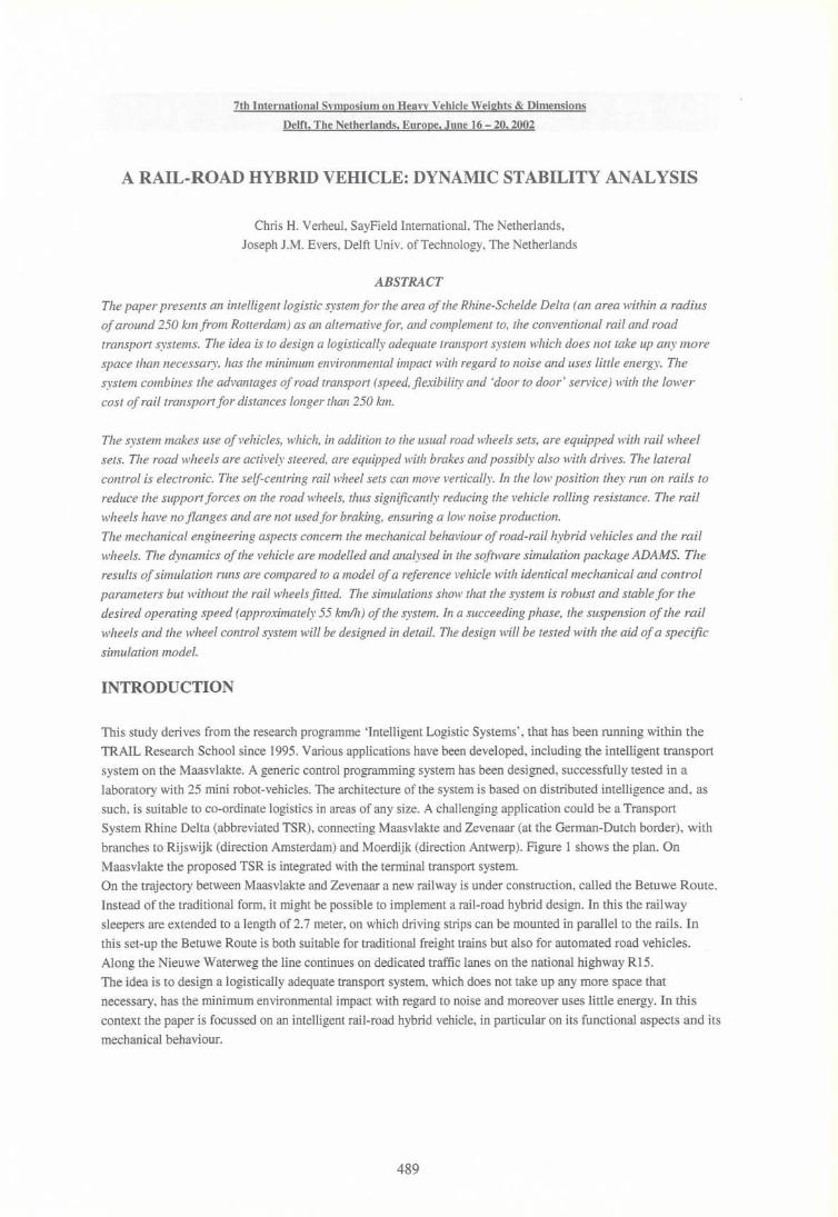
7th International Svmposium on Heavv Vehicle Weights & Dimensions

Delft, The Netherlands, Europe, June 16 - 20, 2002

A RAIL-ROAD HYBRID VEHICLE: DYNAMIC STABILITY ANALYSIS

Chris H. Verheul, SayField International, The Netherlands,

Joseph 1.M. Evers, Delft Univ. of Technology, The Netherlands

ABSTRACT

The paper presents an intelligent logistic system for the area of the Rhine-Schelde Delta (an area within a radius

of around 250 km from Rotterdam) as an alternative for, and complement to, the conventional rail and road

transport systems. The idea is to design a logistically adequate transport system which does not take up any more

space than necessm)l, has the minimum environmental impact with regard to noise and uses little energy. The

system combines the advantages of road transport (speed, flexibility and 'door to door ' service) with the lower

cost of rail transport for distances longer than 250 km.

The system makes use of vehicles, which, in addition to the usual road wheels sets, are equipped with rail wheel

sets. The road wheels are actively steered, are equipped with brakes and possibly also with drives. The lateral

control is electronic. The self-centring rail wheel sets can move vertically. In the low position they run on rails to

reduce the support forces on the road wheels, thus significantly reducing the vehicle rolling resistance. The rail

wheels have no flanges and are not used for braking, ensuring a low noise production.

The mechanical engineering aspects concern the mechanical behaviour of road-rail hybrid vehicles and the rail

wheels. The dynamics of the vehicle are modelled and analysed in the software simulation package ADAMS. The

results of simulation runs are compared to a model of a reference vehicle with identical mechanical and control

parameters but without the rail wheels fitted. The simulations show that the system is robust and stable for the

desired operating speed (approximately 55 kmlh) of the system. In a succeeding phase, the suspension of the rail

wheels and the wheel control system will be designed in detail. The design will be tested with the aid of a specific

simulation model.

INTRODUCTION

This study derives from the research programme 'Intelligent Logistic Systems', that has been running within the

TRAIL Research School since 1995. Various applications have been developed, including the intelligent transport

system on the Maasvlakte. A generic control programming system has been designed, successfully tested in a

laboratory with 25 mini robot-vehicles. The architecture of the system is based on distributed intelligence and, as

such, is suitable to co-ordinate logistics in areas of any size. A challenging application could be a Transport

System Rhine Delta (abbreviated TSR), connecting Maasvlakte and Zevenaar (at the German-Dutch border), with

branches to Rijswijk (direction Amsterdam) and Moerdijk (direction Antwerp). Figure 1 shows the plan. On

Maasvlakte the proposed TSR is integrated with the terminal transport system.

On the trajectory between Maasvlakte and Zevenaar a new railway is under construction, called the Betuwe Route.

Instead of the traditional form, it might be possible to implement a rail-road hybrid design. In this the railway

sleepers are extended to a length of 2.7 meter, on which driving strips can be mounted in parallel to the rails. In

this set-up the Betuwe Route is both suitable for traditional freight trains but also for automated road vehicles.

Along the Nieuwe Waterweg the line continues on dedicated traffic lanes on the national highway R15.

The idea is to design a logistically adequate transport system, which does not take up any more space that

necessary, has the minimum environmental impact with regard to noise and moreover uses little energy. In this

context the paper is focussed on an intelligent rail-road hybrid vehicle, in particular on its functional aspects and its

mechanical behaviour.

489

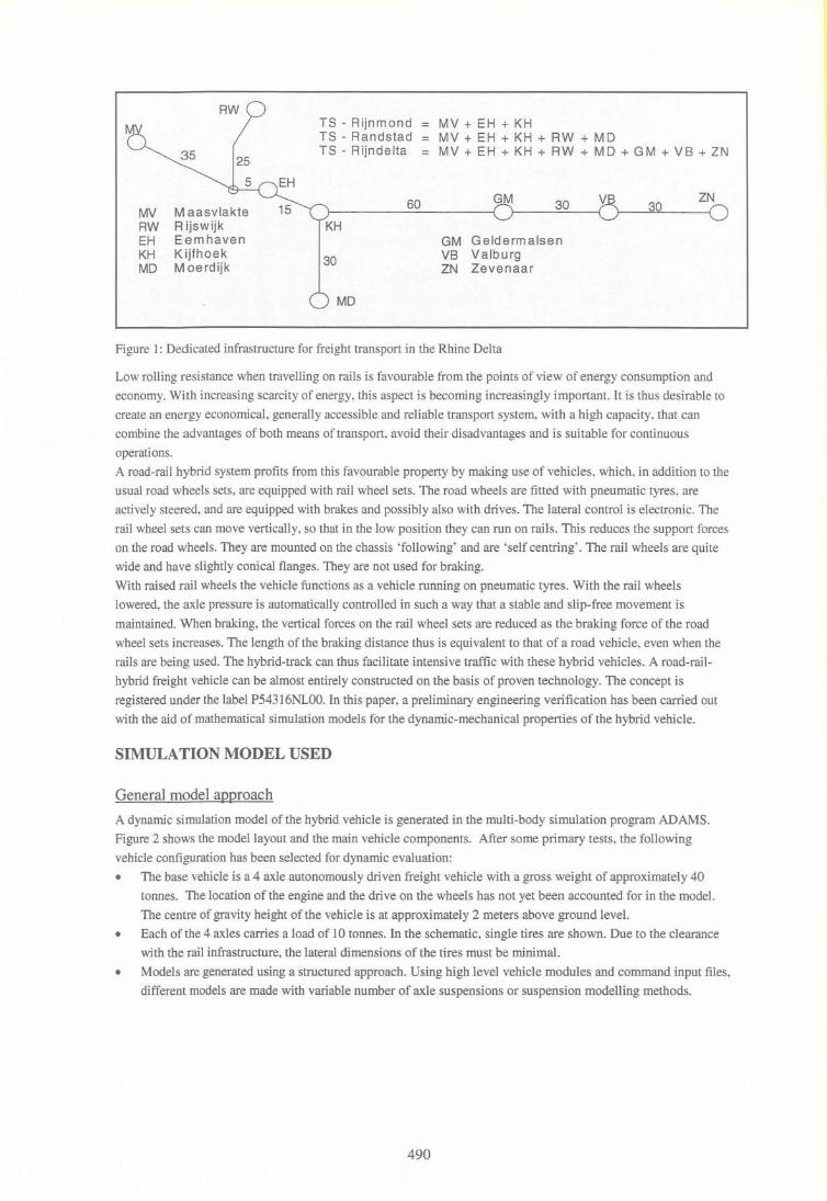
RW

MV M aasvlakte RW R ijswijk EH Eemhaven KH Kijfhoek MD Moerdijk

TS - Rijnmond TS - Randstad TS - Rijndelta

60

MD

MV + EH + KH MV+EH+KH+RW+MD MV + EH + KH + RW + MD + GM + VB + ZN

GM 30

GM Geldermalsen VB Valburg ZN Zevenaar

30 ZN VB

Figure 1: Dedicated infrastructure for freight transport in the Rhine Delta

Low rolling resistance when travelling on rails is favourable from the points of view of energy consumption and

economy. With increasing scarcity of energy, this aspect is becoming increasingly important. It is thus desirable to

create an energy economical, generally accessible and reliable transport system, with a high capacity, that can

combine the advantages of both means of transport, avoid their disadvantages and is suitable for continuous

operations.

A road-rail hybrid system profits from this favourable property by making use of vehicles, which, in addition to the

usual road wheels sets, are equipped with rail wheel sets. The road wheels are fitted with pneumatic tyres, are

actively steered, and are equipped with brakes and possibly also with drives. The lateral control is electronic. The

rail wheel sets can move vertically, so that in the low position they can run on rails. This reduces the support forces

on the road wheels. They are mounted on the chassis 'following' and are 'self centring'. The rail wheels are quite

wide and have slightly conical flanges. They are not used for braking.

With raised rail wheels the vehicle functions as a vehicle running on pneumatic tyres. With the rail wheels

lowered, the axle pressure is automatically controlled in such a way that a stable and slip-free movement is

maintained. When braking, the vertical forces on the rail wheel sets are reduced as the braking force of the road

wheel sets increases. The length of the braking distance thus is equivalent to that of a road vehicle, even when the

rails are being used. The hybrid-track can thus facilitate intensive traffic with these hybrid vehicles. A road-rail­

hybrid freight vehicle can be almost entirely constructed on the basis of proven technology. The concept is

registered under the label P543I 6NLOO. In this paper, a preliminary engineering verification has been carried out

with the aid of mathematical simulation models for the dynamic-mechanical properties of the hybrid vehicle.

SIMULATION MODEL USED

General model approach

A dynamic simulation model of the hybrid vehicle is generated in the multi-body simulation program ADAMS.

Figure 2 shows the model layout and the main vehicle components. After some primary tests, the following

vehicle configuration has been selected for dynamic evaluation:

• The base vehicle is a 4 axle autonomously driven freight vehicle with a gross weight of approximately 40

tonnes. The location of the engine and the drive on the wheels has not yet been accounted for in the model.

The centre of gravity height of the vehicle is at approximately 2 meters above ground level.

• Each of the 4 axles carries a load of 10 tonnes. In the schematic, single tires are shown. Due to the clearance

with the rail infrastructure, the lateral dimensions of the tires must be minimal.

• Models are generated using a structured approach. Using high level vehicle modules and command input files,

different models are made with variable number of axle suspensions or suspension modelling methods.

490

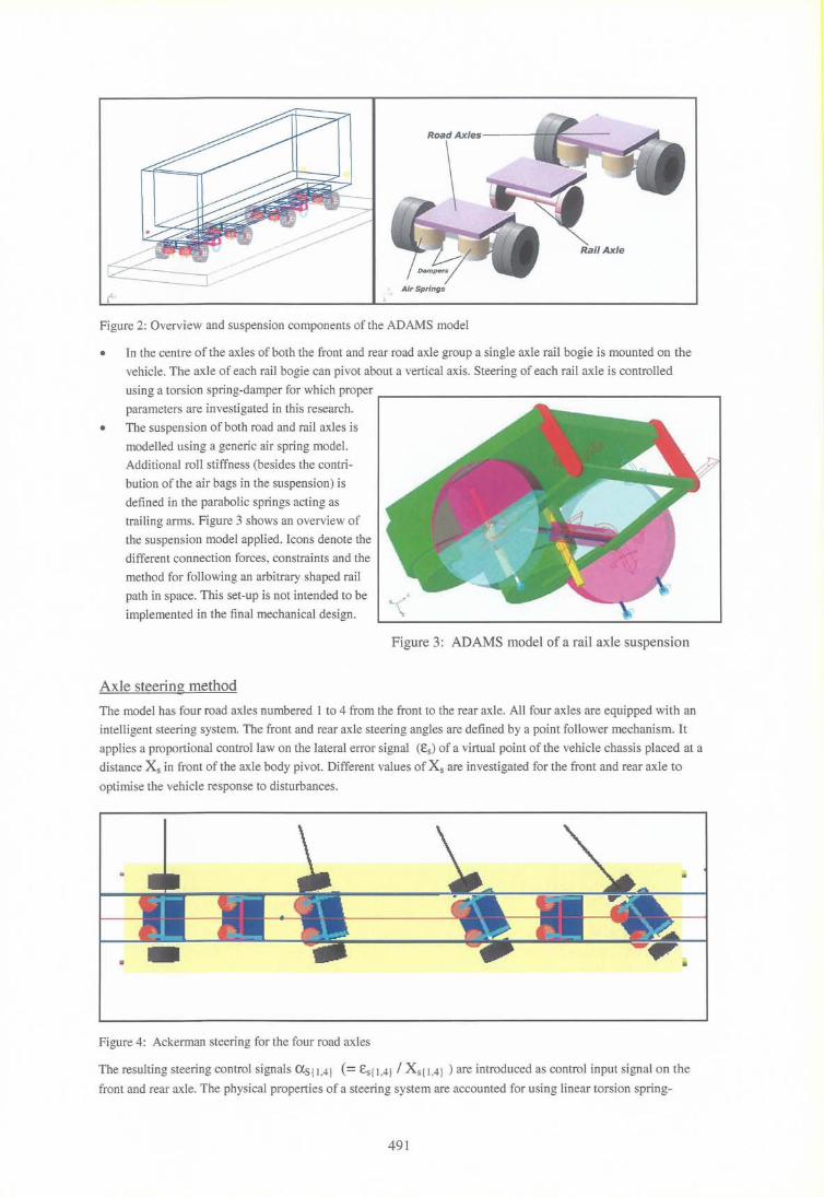
Figure 2: Overview and suspension components of the ADAMS model

• In the centre of the axles of both the front and rear road axle group a single axle rail bogie is mounted on the

vehicle. The axle of each rail bogie can pivot about a vertical axis. Steering of each rail axle is controlled

using a torsion spring-damper for which proper r----------------------------, parameters are investigated in this research.

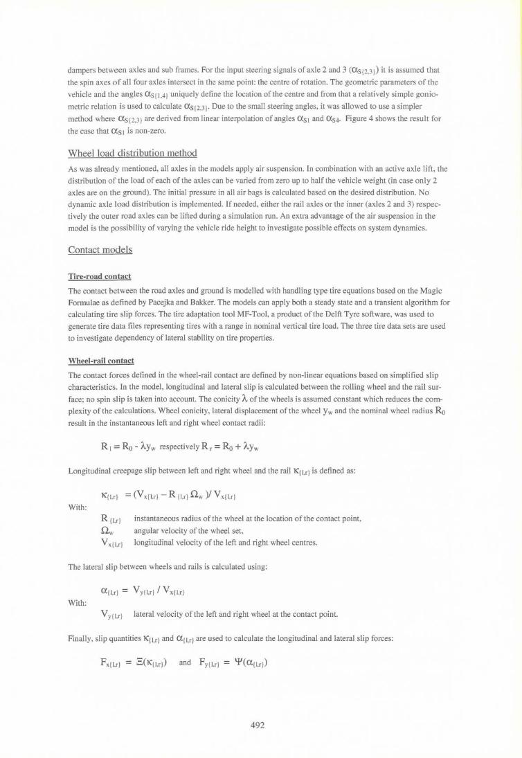
• The suspension of both road and rail axles is

modelled using a generic air spring model.

Additional roll stiffness (besides the contri­

bution of the air bags in the suspension) is

defined in the parabolic springs acting as

trailing arms. Figure 3 shows an overview of

the suspension model applied. Icons denote the

different connection forces, constraints and the

method for following an arbitrary shaped rail

path in space. This set-up is not intended to be

implemented in the final mechanical design.

Axle steering method

Figure 3: ADAMS model of a rail axle suspension

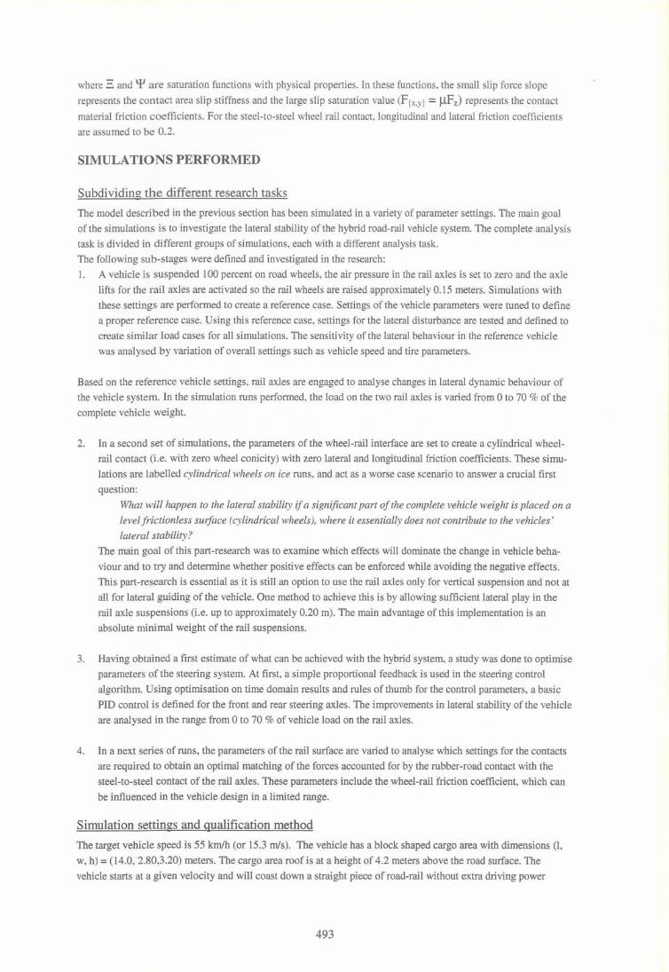
The model has four road axles numbered 1 to 4 from the front to the rear axle. All four axles are equipped with an

intelligent steering system. The front and rear axle steering angles are defined by a point follower mechanism. It

applies a proportional control law on the lateral error signal (c.s) of a virtual point of the vehicle chassis placed at a

distance Xs in front of the axle body pivot. Different values of Xs are investigated for the front and rear axle to

optirnise the vehicle response to disturbances .

•

Figure 4: Ackerman steering for the four road axles

The resulting steering control signals US{lA} (= C.s{lA} / Xs{IA} ) are introduced as control input signal on the

front and rear axle. The physical properties of a steering system are accounted for using linear torsion spring-

491

dampers between axles and sub frames. For the input steering signals of axle 2 and 3 (US{2,3}) it is assumed that

the spin axes of all four axles intersect in the same point: the centre of rotation. The geometric parameters of the

vehicle and the angles US{l,4} uniquely define the location of the centre and from that a relatively simple gonio­

metric relation is used to calculate US{2,3}' Due to the small steering angles, it was allowed to use a simpler

method where CXS{2,3} are derived from linear interpolation of angles USI and US4. Figure 4 shows the result for

the case that aSI is non-zero.

Wheel load distribution method

As was already mentioned, all axles in the models apply air suspension. In combination with an active axle lift, the

distribution of the load of each of the axles can be varied from zero up to half the vehicle weight (in case only 2

axles are on the ground). The initial pressure in all air bags is calculated based on the desired distribution. No

dynamic axle load distribution is implemented. If needed, either the rail axles or the inner (axles 2 and 3) respec­

tively the outer road axles can be lifted during a simulation run. An extra advantage of the air suspension in the

model is the possibility of varying the vehicle ride height to investigate possible effects on system dynamics.

Contact models

Tire-road contact

The contact between the road axles and ground is modelled with handling type tire equations based on the Magic

Formulae as defined by Pacejka and Bakker. The models can apply both a steady state and a transient algorithm for

calculating tire slip forces. The tire adaptation tool MF-Tool, a product of the Delft Tyre software, was used to

generate tire data files representing tires with a range in nominal vertical tire load. The three tire data sets are used

to investigate dependency of lateral stability on tire properties.

Wheel-rail contact

The contact forces defined in the wheel-rail contact are defined by non-linear equations based on simplified slip

characteristics. In the model, longitudinal and lateral slip is calculated between the rolling wheel and the rail sur­

face; no spin slip is taken into account. The coni city A of the wheels is assumed constant which reduces the com­

plexity of the calculations. Wheel conicity, lateral displacement of the wheel Yw and the nominal wheel radius Ra result in the instantaneous left and right wheel contact radii:

RI = Ra - Ayw respectively Rr = Ra + Ayw

Longitudinal creep age slip between left and right wheel and the rail K{l,r} is defined as:

With:

K{l,r} = (V x{l,r) - R {I.r} Q w )/ V x{l,r}

R p,r}

Q w

Vx{l,r}

instantaneous radius of the wheel at the location of the contact point,

angular velocity of the wheel set,

longitudinal velocity of the left and right wheel centres.

The lateral slip between wheels and rails is calculated using:

Up,r} = Vy{I,r} / V x{I,r}

With:

Vy{l,r} lateral velocity of the left and right wheel at the contact point.

Finally, slip quantities K{I,r} and Up,r} are used to calculate the longitudinal and lateral slip forces:

Fx{l,r} = 3(K{I,r}) and Fy{l,r} = 'I'(U{I,r})

492

where =: and q.t are saturation functions with physical properties. In these functions , the small slip force slope

represents the contact area slip stiffness and the large slip saturation value (F {x.y) = JlFz) represents the contact

material friction coefficients. For the steel-to-steel wheel rail contact, longitudinal and lateral friction coeffi cients

are assumed to be 0.2.

SIMULATIONS PERFORMED

Subdividing the different research tasks

The model described in the previous section has been simulated in a variety of parameter settings. The main goal

of the simulations is to investigate the lateral stability of the hybrid road-rail vehicle system. The complete analysis

task is divided in different groups of simulations, each with a different analysis task.

The following sub-stages were defined and investigated in the research:

1. A vehicle is suspended 100 percent on road wheels, the air pressure in the rail axles is set to zero and the axle

lifts for the rail axles are activated so the rail wheels are raised approximately 0.15 meters. Simulations with

these settings are performed to create a reference case. Settings of the vehicle parameters were tuned to define

a proper reference case. Using this reference case, settings for the lateral disturbance are tested and defined to

create similar load cases for all simulations. The sensitivity of the lateral behaviour in the reference vehicle

was analysed by variation of overall settings such as vehicle speed and tire parameters.

Based on the reference vehicle settings, rail axles are engaged to analyse changes in lateral dynamic behaviour of

the vehicle system. In the simulation runs performed, the load on the two rail axles is varied from 0 to 70 % of the

complete vehicle weight.

2. In a second set of simulations, the parameters of the wheel-rail interface are set to create a cylindrical wheel­

rail contact (i.e. with zero wheel conicity) with zero lateral and longitudinal friction coefficients. These simu­

lations are labelled cylindrical wheels on ice runs, and act as a worse case scenario to answer a crucial first

question:

What will happen to the lateral stability if a significant part of the complete vehicle weight is placed on a

level frictionless surface (cylindrical wheels), where it essentially does not contribute to the vehicles'

lateral stability?

The main goal of this part-research was to examine which effects will dominate the change in vehicle beha­

viour and to try and determine whether positive effects can be enforced while avoiding the negative effects.

This part-research is essential as it is still an option to use the rail axles only for vertical suspension and not at

all for lateral guiding of the vehicle. One method to achieve this is by allowing sufficient lateral play in the

rail axle suspensions (i.e. up to approximately 0.20 m). The main advantage of this implementation is an

absolute minimal weight of the rail suspensions.

3. Having obtained a first estimate of what can be achieved with the hybrid system, a study was done to optimise

parameters of the steering system. At first , a simple proportional feedback is used in the steering control

algorithm. Using optimisation on time domain results and rules of thumb for the control parameters, a basic

PlO control is defined for the front and rear steering axles. The improvements in lateral stability of the vehicle

are analysed in the range from 0 to 70 % of vehicle load on the rail axles.

4. In a next series of runs, the parameters of the rail surface are varied to analyse which settings for the contacts

are required to obtain an optimal matching of the forces accounted for by the rubber-road contact with the

steel-to-steel contact of the rail axles. These parameters include the wheel-rail friction coefficient, which can

be influenced in the vehicle design in a limited range.

Simulation settings and qualification method

The target vehicle speed is 55 kmlh (or 15.3 m1s). The vehicle has a block shaped cargo area with dimensions (l,

w, h) = (14.0, 2.80,3.20) meters. The cargo area roof is at a height of 4.2 meters above the road surface. The

vehicle starts at a given velocity and will coast down a straight piece of road-rail without extra driving power

493

activated. The method to maintain constant driving speed is by having zero rolling resistance and zero aero­

dynamic friction forces on the vehicle system.

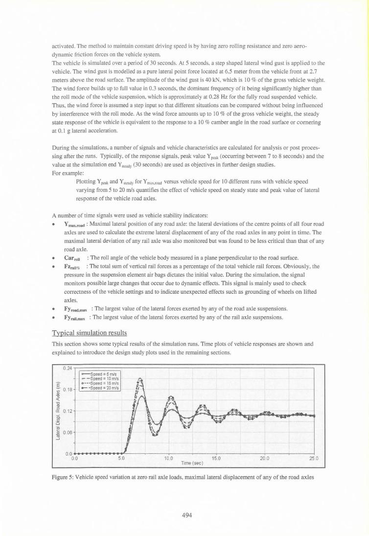
The vehicle is simulated over a period of 30 seconds. At 5 seconds, a step shaped lateral wind gust is applied to the

vehicle. The wind gust is modelled as a pure lateral point force located at 6.5 meter from the vehicle front at 2.7

meters above the road surface. The amplitude of the wind gust is 40 kN, which is 10% of the gross vehicle weight.

The wind force builds up to full value in 0.3 seconds, the dominant frequency of it being significantly higher than

the roll mode of the vehicle suspension, which is approximately at 0.28 Hz for the fully road suspended vehicle.

Thus, the wind force is assumed a step input so that different situations can be compared without being influenced

by interference with the roll mode. As the wind force amounts up to 10 % of the gross vehicle weight, the steady

state response of the vehicle is equivalent to the response to a 10 % camber angle in the road surface or cornering

at 0.1 g lateral acceleration.

During the simulations, a number of signals and vehicle characteristics are calculated for analysis or post proces­

sing after the runs. Typically, of the response signals, peak value Y peak (occurring between 7 to 8 seconds) and the

value at the simulation end Ysteady (30 seconds) are used as objectives in further design studies.

For example:

Plotting Y peak and Y steady for Y max.road versus vehicle speed for 10 different runs with vehicle speed

varying from 5 to 20 mls quantifies the effect of vehicle speed on steady state and peak value of lateral

response of the vehicle road axles.

A number of time signals were used as vehicle stability indicators:

• Y max,road : Maximal lateral position of any road axle: the lateral deviations of the centre points of all four road

axles are used to calculate the extreme lateral displacement of any of the road axles in any point in time. The

maximal lateral deviation of any rail axle was also monitored but was found to be less critical than that of any

road axle.

• Car roll : The roll angle of the vehicle body measured in a plane perpendicular to the road surface.

• FZrai1% : The total sum of vertical rail forces as a percentage of the total vehicle rail forces. Obviously, the

pressure in the suspension element air bags dictates the initial value. During the simulation, the signal

monitors possible large changes that occur due to dynamic effects. This signal is mainly used to check

correctness of the vehicle settings and to indicate unexpected effects such as grounding of wheels on lifted

axles.

• FYroad,max: The largest value of the lateral forces exerted by any of the road axle suspensions.

• FYrail,max: The largest value of the lateral forces exerted by any of the rail axle suspensions.

Typical simulation results

This section shows some typical results of the simulation runs. Time plots of vehicle responses are shown and

explained to introduce the design study plots used in the remaining sections.

O _ 24 ~----------------------------------~------------------------------------~

E 7;;' 0_18

-Speed = 5 mfs .- -Speed = 10 m/s ~---Speed = 15 m/s - -Speed = 20 m{s --:------------------ - --------------------- ------- -.. -----,-------------.----

(])

:z "0 ro 0 0:: 0_12 li (J)

is ~

0_06 ~ -l

0 _0~~~ .. ~~ .. 1L----~------~------~----~------~------~----~------~ 0_0 5_0 10_0 15.0 20 .0 25 _0

Time (sec)

Figure 5: Vehicle speed variation at zero rail axle loads, maximal lateral displacement of any of the road axles

494

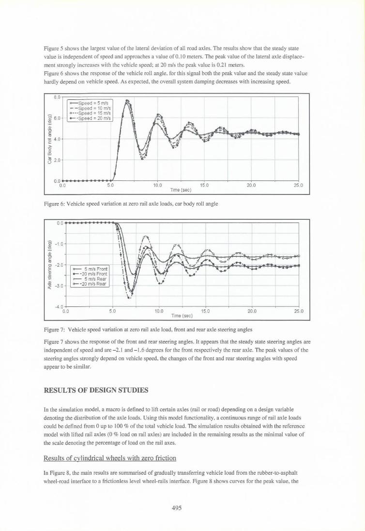
Figure 5 shows the largest value of the lateral deviation of all road axles. The results show that the steady state

value is independent of speed and approaches a value of 0.10 meters. The peak value of the lateral axle displace­

ment strongly increases with the vehicle speed; at 20 m/s the peak value is 0.21 meters.

Figure 6 shows the response of the vehicle roll angle, for this signal both the peak value and the steady state value

hardly depend on vehicle speed. As expected, the overall system damping decreases with increasing speed.

8.0 I,===========;-----::---I--------I--I----~

~ 60 :s-a> DJ c ('iJ

'2 4.0 :>. -0 o co

-Speed = 5 m/s - -'Speed = 10 m/s eo---Speed = 15 m/s - -Speed = 20 m/s

~ 2.0 +-------------~~----_r~~--+_------~-----+------_r------+_------r_----~

O.O~~~~~~~~L-----~------+_------~----_.------~------+_------~----~

0.0 50 10.0 15.0 20.0 25.0 Time (sec)

Figure 6: Vehicle speed variation at zero rail axle loads, car body roll angle

0.0

Ol -1 .0 a> :s-a> DJ c ('iJ

O'l - 2.0 c -·c a>

* ~ -3.0 --L--t------+--

-4.0 0.0 5.0 10.0 15.0 20.0 25.0

Time (sec)

Figure 7: Vehicle speed variation at zero rail axle load, front and rear axle steering angles

Figure 7 shows the response of the front and rear steering angles. It appears that the steady state steering angles are

independent of speed and are - 2.1 and - 1.6 degrees for the front respectively the rear axle. The peak values of the

steering angles strongly depend on vehicle speed, the changes of the front and rear steering angles with speed

appear to be similar.

RESULTS OF DESIGN STUDIES

In the simulation model, a macro is defined to lift certain axles (rail or road) depending on a design variable

denoting the distribution of the axle loads. Using this model functionality, a continuous range of rail axle loads

could be defined from 0 up to 100 % of the total vehicle load. The simulation results obtained with the reference

model with lifted rail axles (0 % load on rail axles) are included in the remaining results as the minimal value of

the scale denoting the percentage of load on the rail axes.

Results of cylindrical wheels with zero friction

In Figure 8, the main results are summarised of gradually transferring vehicle load from the rubber-to-asphalt

wheel-road interface to a frictionless level wheel-rails interface. Figure 8 shows curves for the peak value, the

495

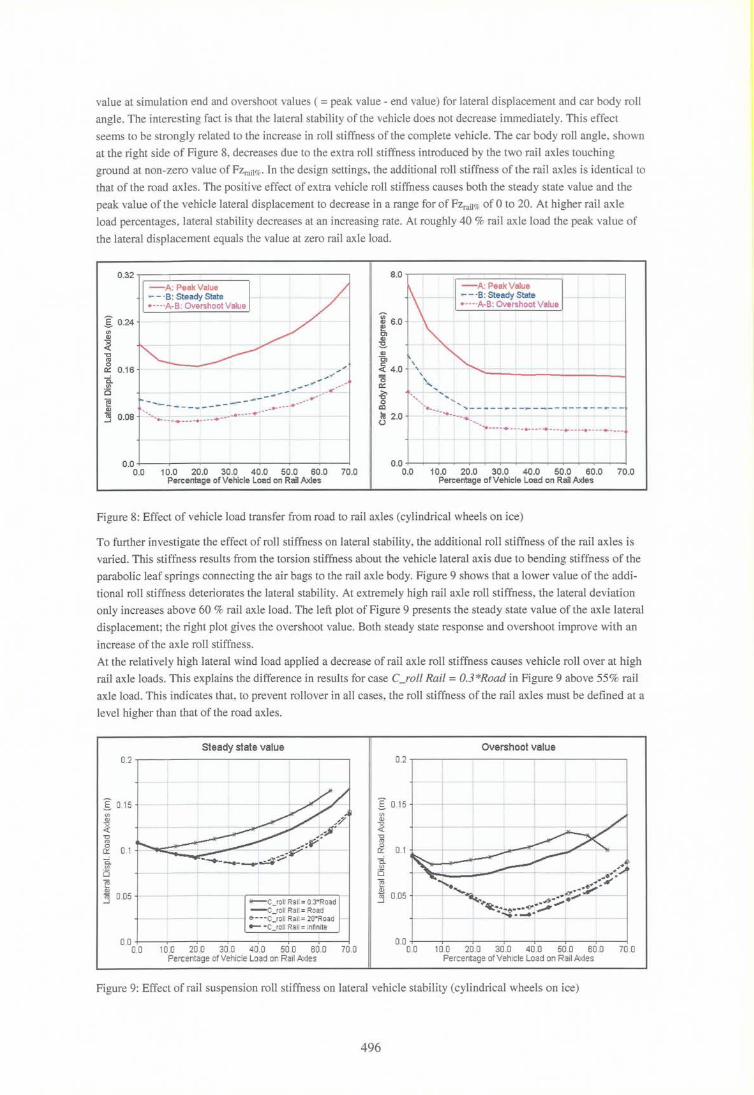
value at simulation end and overshoot values ( = peak value - end value) for lateral displacement and car body roll

angle. The interesting fact is that the lateral stability of the vehicle does not decrease immediately. This effect

seems to be strongly related to the increase in roll stiffness of the complete vehicle. The car body roll angle, shown

at the right side of Figure 8, decreases due to the extra roll stiffness introduced by the two rail axles touching

ground at non-zero value of Fzrail%. In the design settings, the additional roll stiffness of the rail axles is identical to

that of the road axles. The positi ve effect of extra vehicle roll stiffness causes both the steady state value and the

peak value of the vehicle lateral displacement to decrease in a range for of Fzrail% of 0 to 20. At higher rail axle

load percentages, lateral stability decreases at an increasing rate. At roughly 40 % rail axle load the peak value of

the lateral displacement equals the value at zero rail axle load.

0.32 -,---------------,--------,

-A: Peak Value - - - ·B: Steady State

.---·A-B: Overshoot Value

:§: 0.24 VJ Q)

~ -c nI 0

a:: 0.16 C. VJ

is ~ Q) --,.....-~ - ---n; 0.08 ..J

0.0 +---,---,.------,--~--~-~---<

0.0 10.0 20.0 30.0 40.0 50.0 60.0 70.0 Percentage of Vehicle Load on Rail Axles

8.0 1 ---;=============;---1

VJ

~ 6.0 Cl Q)

:s. Q)

Cl ~ 4.0 15 a:: ~ o aJ

~ 2.0 ()

, -,-~ ,

-A: Peak Value - - ·B: Steady State ·---·A-B: Overshoot Value

~ ..... --...... ... '- "' .. ~---.-~-:~ -~ --... ----------== --=

---.. ---,+---- ... ---.. ---- .. ---... ---------I

0.0 +-~-,-~-..--~--,...-~-,.--~-,-~-..--~--1 0.0 10.0 20.0 30 .0 40.0 50.0 60.0 70.0

Percentage of Vehicle Load on Rail Axles

Figure 8: Effect of vehicle load transfer from road to rail axles (cylindrical wheels on ice)

To further investigate the effect of roll stiffness on lateral stability, the additional roll stiffness of the rail axles is

varied. This stiffness results from the torsion stiffness about the vehicle lateral axis due to bending stiffness of the

parabolic leaf springs connecting the air bags to the rail axle body. Figure 9 shows that a lower value of the addi­

tional roll stiffness deteriorates the lateral stability. At extremely high rail axle roll stiffness, the lateral deviation

only increases above 60 % rail axle load. The left plot of Figure 9 presents the steady state value of the axle lateral

displacement; the right plot gives the overshoot value. Both steady state response and overshoot improve with an

increase of the axle roll stiffness.

At the relatively high lateral wind load applied a decrease of rail axle roll stiffness causes vehicle roll over at high

rail axle loads. This explains the difference in results for case C_roll Rail = 0.3 *Road in Figure 9 above 55% rail

axle load. This indicates that, to prevent rollover in all cases, the roll stiffness of the rail axles must be defined at a

level higher than that of the road axles.

Steady state value 0.2 ,------------------,-------,

I 0.15 (fJ (l)

~ -c ro

er

i .:J 0.05 --C_roll Rail = O.3"Road -C_roll Rail = Road ~---C_roll Rail = 20~Road - -C_roll Rail = infinite

0.0 +------.----.,,.----,------,-----.-- ---,-- ----1 00 100 20 .0 30.0 40 .0 50 .0 60 .0 70 .0

Percentage of Vehicle Load on Rail Axles

Overshoot value 0.2 ,-------------------~

I 0.15 (fJ (l)

~ -c tu o

0::: 0.1

0.0 +------,---,.-------.---,.------,-------,---1 00 100 20 .0 30 .0 40 .0 50 .0 60 .0 70 .0

Percentage of Vehicle Load on Rail Axles

Figure 9: Effect of rail suspension roll stiffness on lateral vehicle stability (cylindrical wheels on ice)

496

Effect of wind excitation

A small investigation is performed on the influence of the wind force application. Results not shown indicate a

linear relationship between wind force amplitude and lateral response peak and steady state values. For Figure 10,

the position of the application point of the wind force position was varied in three different rail axle load settings.

The three lines denote the peak values of the largest road axle lateral displacement. Especially at 0 and 30 % rail

axle load, the effect of the wind force location is not large. At approximately 6m behind car front (lm in front of

the car centre) we have a minimum. Furthermore, at 30 % rail axle load, the system lateral stability is still compa­

rable to the reference vehicle with 0 % rail axle load. However, at 60 % rail axle load the peak lateral response

increases significantly for all wind force positions.

i 04 ----------.-.1.. ! -r- i I I _----:-~---------~~--::r:. 0.3 ----+---- -' I ------ I

~- -i-----t-! ----+1-------+- ------------tf-- .... - --- -_- _--....:;c- -=-=.,- --~-.-.--- -..-1;-=-.::...----------... -------+-------+-----.1 ! 02" - - i --- i * - - - ~ - - - -"'1------ ----... -- - -- -

B 0.1 j -0 % on Rail Axles 1 I - - 30 % on Rail Axles I

~ .---60 % on Rail ,Axles 11

"* I I I

.J 1 I 0 . 0 +----~~----.----4-----,-----.----4-----~---~

-8.5 -8.0 -7.5 -7.0 -6 .5 -6.0 -5 .5 -5 .0 -4 .5 Location of lateral wind force (m) (0 = car front)

Figure 10: Effect of wind force application point (cylindrical wheels on ice)

Effect of tire parameters

An important parameter for road tires is the characteristic of the lateral slip stiffness versus the vertical load on the

tire. Figure 11 shows three characteristics for different values of the tire nominal vertical load. This nominal load

can be considered as the vertical load where a tire is designed to operate in. The dark vertical lines denote the

average tire load in each tire at 0 and 60 % vehicle load on rail axles.

c 0

r n e r

n g

i f f n e

N I d e g

*le3

0

-1

-2

-3

-4

-5

-6

-7

Tire Slip Stiffuess vs Fz for 3 Tires: Fnorn = 60 KN~ 80 KN and 100 KN - -~ - 1- - ~ -T-Tire lo~d at 60 % load on Rails I I

o 20

I T i 1--lire load at 0 % loaa oilRails

+

40 60 80 100 120

Vertical load -N -

F _no~ = 100 KN

140 160 *le3

Figure 11 : Three tire characteristics with variation of lateral slip stiffness versus vertical load

Due to lateral tire forces, (i.e. while curving or during a lateral wind) a wheel load transfer will take place from one

side of the vehicle to the other. Due to this load transfer, the wheel loads left and right will be evenly distributed at

497

both sides of the solid vertical lines in Figure 11. The resulting decrease of the effective axle lateral slip stiffness

depends on the amount of load transfer and the curvature of the tire slip stiffness versus tire vertical load. Figure 11

thus gi ves one explanation of the increased lateral stability at increased rail axle roll stiffness. A decrease in road

wheels load transfer left-right reduces the decrease of axle sideslip stiffness, which increases the lateral vehicle

stability.

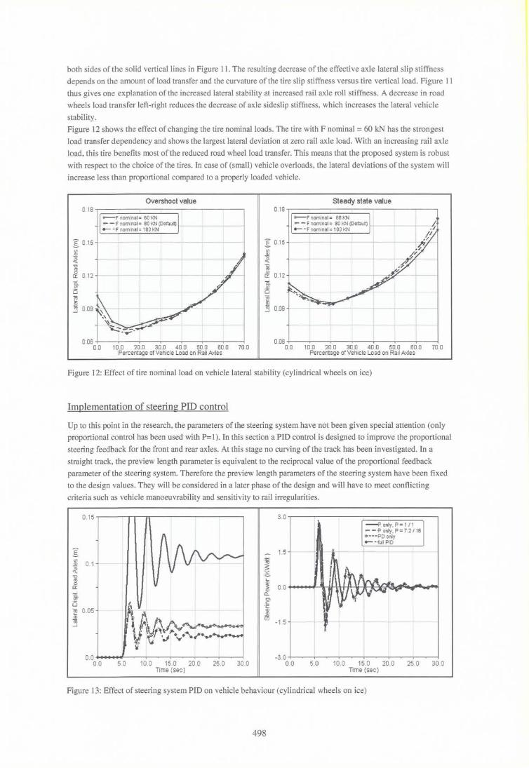
Figure 12 shows the effect of changing the tire nominal loads. The tire with F nominal = 60 kN has the strongest

load transfer dependency and shows the largest lateral deviation at zero rail axle load. With an increasing rail axle

load, this tire benefits most of the reduced road wheel load transfer. This means that the proposed system is robust

with respect to the choice of the tires. In case of (small) vehicle overloads, the lateral deviations of the system will

increase less than proportional compared to a properly loaded vehicle.

Overshoot value

0.18 Tr=============~----:----I -F nominal = 60 KN - - ·F nominal = 80 KN (Default) ~

I 0.15

- -·F nominal = 100 KN I

---f=~ (fJ

~ -0 ro o

0::: 0.12

~ (5 ro

I

---l-----

~ ....J 0.09

0.06 +---___,_--.----.---~--..,.-----,------I

0.0 10.0 20.0 30 .0 40 .0 50 .0 60.0 70 .0 Percentage of Vehicle Load on Rail Axles

Steady state value 0.18 .,------- --- - ---------,

-F nominal = 60 KN _ - - ·F nominal = 80 KN (Default) I-t---+-----t

- -·F nominal = 100 KN

I O.15-t---+--(fJ

~ -0 ro o

0::: 0.12

~ (5 ro ID .!3 0.09 -j-----,---i---->---ii----t-- -+----(

0.06 +--- ---,-- -,----.-----;r----.------.----i 0.0 100 20 .0 30 .0 40 .0 50 .0 60 .0 70 .0

Percentage of Vehicle Load on Rail Axles

Figure 12: Effect of tire nominal load on vehicle lateral stability (cylindrical wheels on ice)

Implementation of steering PID control

Up to this point in the research, the parameters of the steering system have not been given special attention (only

proportional control has been used with P=I). In this section a PID control is designed to improve the proportional

steering feedback for the front and rear axles. At this stage no curving of the track has been investigated. In a

straight track, the preview length parameter is equivalent to the reciprocal value of the proportional feedback

parameter of the steering system. Therefore the preview length parameters of the steering system have been fixed

to the design values. They will be considered in a later phase of the design and will have to meet conflicting

criteria such as vehicle manoeuvrability and sensitivity to rail irregularities.

0.15 3.0 -P only, P = 1 1 1 - -P only , P = 7.2 / 16 &---PO only --full PlO

I 1.5 (J) :l=i Q) 0. 1 (IJ

~ 5 -0 ~ (IJ '-0 Q)

0::: $ 00 0

~ 0.. Cl

(5

A c ·c

~ 0.05 ~-jo\\ A - Q)

Q)

.$ U5 - 1.5 (IJ

\r~,~~~~~ ....J

~r 'w1 ,.1 .............................. ~

0.0 -3.0 0.0 5.0 10.0 15.0 20 .0 25 .0 30 .0 00 5.0 10.0 15.0 20 .0 25 .0 30.0

Time (sec) Time (sec)

Figure 13: Effect of steering system PID on vehicle behaviour (cylindrical wheels on ice)

498

Using a practical iterative approach, reasonably optimal PID parameters for the steering system of front and rear

road axles are assessed. This resulted in (PII/O) = (7.2/8.012.7) for the front axle and (PII/O) = (16.0/5.0/4.0) for

the rear axle. Figure 13 shows the results of the vehicle lateral stability in a number of phases of PlO design. It is

clear that while the lateral deviation of the vehicle is drastically reduced, the power consumption of the steering

system is hardly affected. The same wind gust as before (at 6.5 m) has been used. The results shown in Figure 13

indicate that the biggest lateral deflection of the road axles can be reduced to a peak value of O.05m and a steady

state value of 0.025m. The current design of the vehicle assumes a lateral play of the rail axles of approximately

0.1 meters. This means that even at this large lateral excitation, the amount of play in the rail axles is still

sufficient. Therefore low lateral forces in the rail axles can be expected. In the next sections this will be verified.

Using rail axles for extra lateral guidance

The results of the simulation runs discussed before indicate that at proper system parameters the lateral stability of

the vehicle can be controlled quite well. The results of the above simulations must be considered as worst case as

no slip forces are being generated between wheel and rail. In this section, realistic wheel-rail frictional contact will

be considered and the effect of conicity will be investigated. A further improvement of system behaviour is expec­

ted because the rail axles will now actively contribute in the lateral suspension as well. The simulations will be

used to indicate the cost: how big are the lateral forces applied on the rail axles to obtain a certain improvement.

This knowledge will be used in the design of the hybrid system.

0.15 ~----------------------------------~------------------------~~------~

g 0.125 (f)

ID x III -0 III o

c:::: 0.1 i5.. (f)

'6

~ -*i 0.075 -/----...J

"-

-Peak Value - - -Steady State

.... .... ~-:"""-C---~---- - -'- - -

0.05 +-----------------.-----------------.-------~--------.---------~------~

0.0 0.0125 0.025 0.0375 0.05 Rail Wheels Coni city

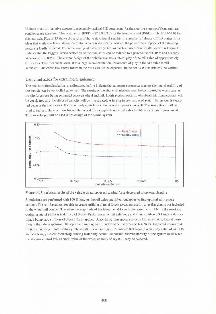
Figure 14: Simulation results of the vehicle on rail axles only, wind force decreased to prevent flanging

Simulations are performed with 100 % load on the rail axles and lifted road axles to find optimal rail vehicle

settings. The rail forces are not able to create sufficient lateral forces to counteract 0.1 g, as flanging is not included

in the wheel-rail contact. Therefore the amplitude of the lateral wind force is decreased to 4.0 kN. In the resulting

design, a lateral stiffness is defined of 3.0e4 N/m between the rail axle body and vehicle. Above 0.1 meters deflec­

tion, a bump stop stiffness of 3.0e7 N/m is applied. Also, the system appears to be rather sensitive to lateral dam­

ping in the axle suspension. The optimal damping was found to be of the order of le4 Ns/m. Figure 14 shows that

limited conicity promotes stability. The results shown in Figure 15 indicate that beyond a coni city value of ca. 0.15

an increasingly violent oscillatory hunting instability occurs. To ensure inherent stability of the system (also when

the steering control fails) a small value of the wheel conicity of say 0.01 may be selected.

499

Variation of Wheel tangent at full car loaded on Rails

(i) Q.l

0 .001 11' ~ 1111 11' 111I1I

~ O.O ~~~~~~~~~~--~------~~~----------------------------------~~~~ ~ -2.5E-004 Q.l

~ 'ffi 0::: C .g Q.l

:5 '0 Q.l 0,

s:::: ro .Q­U5

-0.0015

-0.00275

--Tang = 0.01 - - - ~ar J : I

--Tang = 0 07

-Tang = 0.16 -- - -Tang = 0.20

r-f -0.004+-----~------~----~----~------~----~----~------~----~~~~

0.0 5 .0 10.0 15.0 20.0 25 .0 Time (sec)

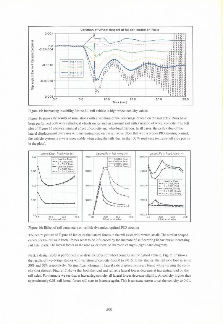
Figure 15: Increasing instability for the full rail vehicle at high wheel conicity values

Figure 16 shows the results of simulations with a variation of the percentage of load on the rail axles. Runs have

been performed both with cylindrical wheels on ice and on a normal rail with variation of wheel conicity. The left

plot of Figure 16 shows a minimal effect of conicity and wheel-rail friction . In all cases, the peak value of the

lateral displacement decreases with increasing load on the rail axles. Note that with a proper PlO steering control,

the vehicle system is always more stable when using the rails than in the 100 % road case (extreme left side points

in the plots).

Lateral Displ. Road Axles (m) 0.06 ~-----;=======::l

0.045

0.03

0.015

-Level Ice, Peak - - ·C = 0.005, Peak ~ --- C = 0 010 Peak - --Level 'lce, Steady -C = 0.005 , Steady lI- - ·C = 0.010, Steady

0.0 +-------.-----------,,---------{ 0.0 25.0 50.0

% load on rail axles 75.0

Largest Fy in Rail Axles (N) 4000.0 -,--------;======='il

3000.0

2000.0

1000.0

- - 'C=O 005 Peak eo - - - C=O:OlO: Peak +--C=0.005, Steady

f>- lI- - ·C=0.010, Steady J,.. .....

,'I ,

/1 ~\ .1 \ '\

IJ ~ "\ \ ..,. ~ ...

----4-_~~

'Q." ... '"""'"X

''El. - -G.-6> __ o

25.0 50.0 % load on ra il axles

75.0

Figure 16: Effect ofrail parameters on vehicle dynamics, optimal PID steering

Largest Fy in Road Axles (N ) 20000.0 -,-----------------------,

17500.0

-Level Ice, Peak

15000.0 - :-_:-~g ~ ~~~~' ~::~ - · ·Level ·lce, Steady +--C = 0.005, Steady

----- lI- _ ·C = 0.010 , Steady -

12500.0 ____ i

10000.0 -+-------,------..,----------1 0.0 25.0 50.0 75.0

% load on rail axles

The centre picture of Figure 16 indicates that lateral forces in the rail axles will remain small. The similar shaped

curves for the rail axle lateral forces seem to be influenced by the increase of self centring behaviour at increasing

rail axle loads. The lateral forces in the road axles show no dramatic changes (right-hand diagram).

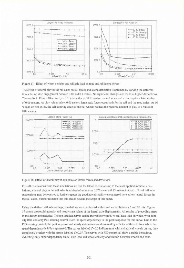
Next, a design study is performed to analyse the effect of wheel conicity on the hybrid vehicle. Figure 17 shows

the results of two design studies with variation of conicity from 0 to 0.015. In the studies, the rail axle load is set to

30% and 60% respectively. No significant changes in lateral axle displacements are found while varying the coni­

city (not shown). Figure 17 shows that both the road and rail axle lateral forces decrease at increasing load on the

rail axles. Furthermore we see that at increasing conicity all lateral forces decrease slightly. At coni city higher than

approximately 0.01, rail lateral forces will start to increase again. This is an extra reason to set the conicity to 0.01.

500

Largest Fy Road Axles (N) 20000 .0 ,------- -----,-----------,

17500 .0

15000.0

···············i···

- 30 % Peak ..... ~ - 30 %: Steady

<:;---60 %, Peak . ... - 60 %, Steady

1 0000 .0 +---~----jr-------T-----,---->--------1 0.0 0.005 0.01 0.015

W heel Coni city

Largest Fy Raill\xles (N) 10000 .0 .---~----------------,

7500.0

50000

2500.0

\ 1

\ ., .... \ 1

,

\ .

-30 %, Peak - -'30 % , Steady eo ---60 %, Peak

···· ·······················1 _ -'60 %, Steady

.................. ' .......................... .......... ..... .. .... ....... ..... ' .. ... .

.... . ~ .... l. .. \ '\

"\ ;, .. ~'\\ ..... :.~""< .................................................. : ....................................... . .. ·· ·t:,~~~-~~~;~'~:::~::b::··

0.0 +-----i-----r- --..----j-------,,__----{

00 0.005 0.01 0.01 5 W heel Coni city

Figure 17: Effect of wheel conicity and rail axle load on road and rail lateral forces

The effect of lateral play in the rail axles on rail forces and lateral deflection is obtained by varying the deforma­

tion at bump stop engagement between 0.01 and 0.1 meters. No significant changes are found at higher deflections.

The results in Figure 18 (conicity = 0.01) show that at 30 % load on the rail axles, rail axles require a lateral play

of 0.06 meters. At play values below 0.06 meters, large peak forces occur both for the rail and the road axles. At 60

% load on rail axles , the self-centring effect of the rail wheels reduces the required amount of play to a value of

0.02 meters.

Largest lateral Forces (N) 30000 .0 -r------:----:-r======= ::::;--,

~ , ,. , ,.

20000.0 ,,1 "...... #Q.

........... (!)! ............. ;.lo.~. :.: . .:.: .~ .... ~ "" ........ ,o---o()---~---o---o()-----_._----------------10000 0 -I ................................•...................................•...............................•...... ··········· ··············1

" "-~-----~----~ -----0.0 +-----,-----;-------;--------1

00 0.025 0.05 0.075 0.1 Lateral play in rail axles (m)

Largest lateral deformation/displacement rail axles (m) 0.1 ~--------;:=====::::;;-]

0.05

0.025 -l ........... -- ......... .

00 +-----,-- ----i-----;------1 0 0 0.025 0.05 0.075 0 .1

Lateral play in rail axles (m)

Figure 18: Effect of lateral play in rail axles on lateral forces and deviations

Overall conclusions from these simulations are that for lateral excitations up to the level applied in these simu­

lations, a lateral play in the rail axles is advised of more than 0.075 meters (0.15 meters in total). Novel rail axle

suspensions may be required to further support the good lateral stability encountered here at low lateral forces in

the rail axles. Further research into this area is beyond the scope of this paper.

Using the defined rail axle settings, simulations were performed with speed varied between 5 and 20 m1s. Figure

19 shows the resulting peak- and steady state values of the lateral axle displacement. All results of preceding steps

in the design are included. The top labelled curves denote the vehicle with 60 % rail axle load on wheel with coni­

city 0.01 and only P=1 steering control. Note the speed dependency in the peak response for this curve. Due to the

PID steering control, the peak response and steady state values are decreased by a factor of three to four while the

speed dependency is fully suppressed. The curves labelled C=O.O indicate runs with cylindrical wheels on ice, they

completely overlap with the results labelled C=O.OI. The curves with PID control all show a stable behaviour,

indicating only minor dependency on rail axle load, rail wheel conicity and friction between wheels and rails.

501

Peak value of axle lateral displacement (m) Steady state value of axle lateral displacement (m) 0.25 r;:::========;-----------, 0 25

lI----\30 % Ra il , C=O.O·I, P=1 - - 0 % Rail , PlO @II---SO % Rail C=O 0 PlO - -60 % Rail: C=0:01, PlO

0 2 ~L-~~~-~-J · 0.2

01 5 0 15 ................ , ............... ............... ' ................ , ....... .

0.1 0.1

0.05 - .~.- .-. ,.,.. .. - ~.- .- ~.- . _x- .- . ...... - -~ .- ~ -.-.~-. 0.05 . ...

. \ ~ ~ ~-~-~~-~4-~-4--~-~~-~+-~-~ ~ ........... ~: ..... -+ ....... --+~.~ .... -....

00 +---~---r------,__--;------l 0.0 5.0 5.0 10 0 15.0 200 10.0 15 0 20.0

Vehicle speed (m/s) Vehi cle speed (m/s)

Figure 19: Effect of vehicle speed on lateral stability, variation of steering PlO, axle load and rail contact

CONCLUSIONS

From the analysis and simulations described, the following conclusions may be drawn:

• A system has been presented and described with high potential for novel use of (partly) existing infrastruc­

ture. The presented system combines the benefits of a rail vehicle (low rolling resistance) with the benefits of

a road vehicle (flexibility in manoeuvring).

• For the expected range of operating velocities of the hybrid vehicle the dynamic simulations have not indica­

ted major dynamics problems. The vehicle system, based on a standard set of vehicle parameters demonstrates

a predictable response to large lateral disturbances.

• A large number of dynamic simulation runs is performed to investigate the effects of reducing the weight on

rubber tires versus the weight on rail-wheels. Conclusions of these simulations are:

o Using a straight forward steering feedback mechanism (with proportional control only) it is possible

to control the lateral stability of the vehicle.

o The lateral stability of the vehicle is dominated by the increase of roll stiffness due to the rail axles

suspensions. Extremely large roll stiffness values can even improve vehicle stability up to a large

amount of road axle unloading.

o In general, the system proposed seems to behave robustly with respect to tire mismatch problems.

o The steering system improves dramatically by implementation of a reasonably simple PID control

strategy. Applying one single strategy for the different vehicle settings already gives a large

reduction of the vehicle lateral displacements. Further improvement may be possible with more

advanced control strategies (self learning, case dependent control settings).

o The extra lateral stabilisation of the vehicle system from lateral guidance of the rail infrastructure

(through conicity) appears to be relatively small. In combination with the need for an extremely

light rail axle construction, this leads to the proposal to design rail axles systems that do not account

for any lateral guidance forces at all.

• An automated approach for modelling complex vehicle systems is strongly advised for performing a compli­

cated full-vehicle analysis as described in this paper. Working in a macro oriented manner with adequate

separation of model data (design variables) and model topology/functionality (model components) enables

users to perform large and complex simulations at a high quality level.

502

• J.J.M. Evers, G.J.M van der Wielen, M.B. Duinkerken, lA. Ottjes. The jumbo container terminal: quay

transport during ship loading. TRAIL Research school, Delft Univ. of Technology, TRAIL/98/308, 1998.

• J.lM. Evers, D.G. Lindeijer. The system for function-oriented machine programming: FORCES.

TRAIL/O I /Feb

• J.J.M. Evers, S. Koppers. Automated guided vehicle traffic-control at a container Transportation Research

(A), January 1996.

• J.J.M. Evers, D.G. Lindeijer. The agile traffic-control and engineering system: TRACES. TRAIL/99/Nov

1999

• J.lM. Evers, G.J.M van der Wielen, M.B. Duinkerken, J.A. Ottjes. The jumbo container ship loading. TRAIL

Research school, Delft University of Technology, TRAIL/98/- Gemeentelijk Havenbedrijf Rotterdam, 1998,

Integrale verkenningen voor haven en industrie 2020, Rotterdam

• J.J .M. Evers. Intelligent Road-Rail-Hybrid Transport: a new transportation modality. TRAIL, January 2001

• H.B. Pacejka (Ed.). Tyre Models for Vehicle Dynamics Analysis . Proceedings of the 2nd International

Colloquim on Tyre Models for Vehicle Dynamics Analysis held in Delft, The Netherlands, October 1991 .

Supplement to Vehicle System Dynamics, Volume 21, AmsterdarnlLisse, 1993, Swets & Zeitlinger.

503

504