A Randomised Kinodynamic Planner

for Closed-chain Robotic SystemsRicard Bordalba, Lluís Ros, and Josep M. Porta

Abstract—Kinodynamic RRT planners are effective tools forfinding feasible trajectories in many classes of robotic systems.However, they are hard to apply to systems with closed-kinematicchains, like parallel robots, collaborative arms manipulating anobject, or legged robots keeping their feet in contact with theenvironment. The state space of such systems is an implicitly-defined manifold that complicates the design of the sampling andsteering procedures, and leads to trajectories that drift from themanifold if standard integration methods are used. To addressthese issues, this paper presents a kinodynamic RRT planner thatconstructs an atlas of the state space incrementally, and uses thisatlas to generate random states, and to dynamically steer thesystem towards such states. The steering method exploits theatlas charts to compute locally optimal policies based on linearquadratic regulators. The atlas also allows the integration of theequations of motion as a differential equation on the manifold,which eliminates any drift from such manifold and results inaccurate trajectories. To the best of our knowledge, this is thefirst kinodynamic planner that explicitly takes closed kinematicchains into account. We illustrate the planner performance insignificantly complex tasks, including planar and spatial robotsthat have to lift or throw a load at a given velocity using torque-limited actuators.

Index terms—Kinodynamic motion planning, loop-closure con-straint, closed kinematic chain, atlas, manifold, LQR, steering.

I. INTRODUCTION

SINCE its formalization in the early nineties [1], the

kinodynamic planning problem remains as one of the

most challenging open problems in robotics. The problem

entails finding feasible trajectories connecting given states

of a robot, each defined by a configuration and a velocity

of the underlying mechanical system. To ensure feasibility,

the trajectory should: 1) fulfil all kinematic constraints of

the system, including holonomic ones, like loop-closure or

end-effector constraints, or nonholonomic ones, like rolling

contact or velocity limit constraints; 2) be compliant with the

equations of motion of the robot; 3) avoid the collisions with

obstacles in the environment; and 4) be executable with the

limited force capacity of the actuators. In certain applications,

moreover, the trajectory should also be optimal in some sense,

minimising, for example, the time or control effort required for

its execution.

This work has been partially funded by the Spanish Ministry of Science,Innovation, and Universities under project DPI2017-88282-P

Ricard Bordalba, Lluís Ros, and Josep M. Porta are with the Institutde Robòtica i Informàtica Industrial (CSIC-UPC). Llorens Artigas 4-6, 08028Barcelona, Catalonia. E-mails: rbordalba@iri.upc.edu, ros@iri.upc.edu, andporta@iri.upc.edu.

The ability to plan such trajectories is key in a robotic sys-

tem. Above all, it endows the system with a means to convert

higher-level commands—like “move to a certain location”, or

“throw the object at a given speed”—into appropriate reference

signals that can be followed by the actuators. By accounting

for the robot dynamics and force limitations at the planning

stage, moreover, the motions are easier to control, and they

often look more graceful, or physically natural [2], as they

tend to exploit gravity, inertia, and centripetal forces to the

benefit of the task.

The kinodynamic planning problem can be viewed as a full

motion planning problem in the state space, as opposed to

a purely kinematic problem that only requires the planning

of a path in configuration space (C-space). This makes the

problem harder, as the dimension of the state space is twice

that of the C-space. Moreover, the obstacle region is virtually

larger, involving states that correspond to an actual collision,

but also those from which a future collision is inevitable due

to the system momentum. The planning of steering motions

is considerably more difficult as well. While direct motions

suffice in the C-space, steering motions in the state space need

to conform to the vector fields defined by the equations of

motion and to the actuator limits of the robot.

Among all kinodynamic planning techniques, rapidly-

exploring random trees (RRTs) have emerged as one of the

most successful planning paradigms to date [7]. RRTs make

intensive use of sampling and dynamic simulations to grow tra-

jectory trees over the state space until the start and goal states

get connected. The efficiency of the approach is remarkable,

especially in view of its simplicity and relative ease of im-

plementation. The technique is fairly general and, with proper

extensions, can even converge to minimum-cost motions [8, 9].

However, existing RRT methods also suffer from a main

limitation: they assume that the robot state can be described

by means of independent generalised coordinates. This makes

them applicable to open-chain robots, or to robots with explicit

state space parametrisations, but they have problems in dealing

with general mechanisms with closed-kinematic chains. Such

chains arise frequently in today’s robots and manipulation

systems (Fig. 1), which explains the growing interest they

arouse in the recent literature [10]–[16].

Unlike in the open-chain case, the state space of a closed-

chain robot is not flat anymore. Instead, it is a nonlinear

manifold defined implicitly by a system of equations that, in

general, cannot be solved in closed form. This manifold is a

zero-measure set in a larger ambient space, which complicates

the design of sampling and steering methods to explore the

manifold efficiently. Moreover, if the dynamic model of the

Fig. 1. Example systems involving closed kinematic chains. The chains may be intrinsic to the robot structure, as in parallel robots (left picture), or theymay result from manipulation constraints during a task, as in multi-limb systems transporting an object, or keeping feet attached to the environment (rightpictures). From left to right: A Delta parallel robot [3], the Atlas robot from Boston Dynamics lifting a heavy load [4], the Robonaut 2 robot with two legsclamped to the International Space Station [5], and the SpiderFab Bot, a conceptual design for self-fabricating space systems [6]. Pictures courtesy of ABB,Boston Dynamics, NASA, and Tethers Unlimited, Inc (respectively).

robot is not properly handled, the planned trajectories may

deviate substantially from the manifold, leading to undesired

violations of the kinematic constraints, or to failure to reach

the goal. Forward singularities may also complicate the plan-

ning and control of motions across certain surfaces of the state

space [17].

The purpose of this paper is to extend the planner in [7]

to cope with the previous complications. As we shall see,

by constructing an atlas of the state space in parallel to the

RRT, one can define proper sampling and steering methods

that deal with closed kinematic chains effectively, while pro-

ducing feasible trajectories even across forward singularities.

An early version of our planner was presented in [18]. In

contrast to [18], we here develop a steering method based on

linear quadratic regulators (LQR), which greatly increases the

planner efficiency in comparison to the randomised strategy

used in [18]. New challenging test cases are also reported

for demonstration, including tasks that require the throwing

of objects at a given velocity, and bimanual manipulations

of heavy loads, which were difficult to solve with [18]. It

is worth noting that, while some path planning approaches

have previously dealt with closed kinematic chains [10]–

[12, 15, 19]–[23], none of them has considered the dynamics

of the system into the planner. Our kinodynamic planner, in

fact, can also be seen as an extension of the work in [12] to

cope with dynamic constraints.

The rest of the paper is organised as follows. Section II

reviews the state of the art on kinodynamic planning to better

place our work into context. Section III formally states the

problem we confront, enumerating our assumptions and the

various constraints intervening. Section IV explains why most

RRT approaches, while powerful, are limited in some way or

another, and would be difficult to extend to cope with closed

chains and dynamic constraints simultaneously. Sections V

and VI present effective sampling, simulation, and steering

methods that allow us to describe, in Section VII, our planner

implementation. Sections VIII and IX respectively examine the

completeness properties of the planner and its practical per-

formance in illustrative situations. Section X finally provides

the paper conclusions and discusses several points requiring

further attention.

II. RELATED WORK

A. C-space approaches

The sheer complexity of kinodynamic planning is usually

managed by decomposing the problem into two simpler prob-

lems [24]. Initially, the dynamic constraints of the robot are

neglected and a collision-free path in the C-space is sought

that solely satisfies the kinematic constraints. Then, a time-

parametric trajectory constrained to the previous path is de-

signed while accounting for the dynamic constraints and force

limits of the actuators. Although many techniques can be used

to compute the path, like probabilistic roadmaps or randomised

tree techniques among others [24, 25], the trajectory is usually

obtained with the time-scaling method in [26] or its later

improvements [27]–[30]. This method regards the path as a

function qqq = qqq(s) in which qqq is the robot configuration and

s is some path parameter, and then finds a monotonic time

scaling s = s(t) such that qqq(t) = qqq(s(t)) connects the start and

goal configurations in minimum time. The method is fast and

elegant, as it exploits the bang-bang nature of the solution in

the (s, s) plane, and robust implementations have recently been

obtained [31].

The previous approach generates a trajectory that is only

time-optimal for the computed path, but makes the problem

more tractable, so it can be solved in systems with many

degrees of freedom like humanoids, legged robots, or mobile

robot formations [32]. Its lack of completeness, moreover, can

be alleviated by improving the trajectory a posteriori using

optimization techniques [33]–[35]. Time scaling methods, in

addition, have recently been extended to compute the feasible

velocities at the end of a path, given an initial range of

velocities [36], which can be combined with randomised

planners to generate graceful dynamic motions [32].

It must be noted that, despite their advantages, the previous

methods essentially work in the C-space, which makes them

limited in some way or another. For instance, path planning

approaches cannot generate swinging paths in principle, and

such paths may be required in highly dynamic tasks like

lifting a heavy load under strict torque limitations. In other

approaches, start or goal states with nonzero velocity cannot

be specified, which is necessary in, e.g., catching or throwing

objects at a certain speed and direction. Time scaling methods,

moreover, require the robot to be fully actuated. While this

is rarely an issue in robot arms or humanoids under contact

constraints [13, 14], parallel robots with passive joints are un-

deractuated at forward singularities [17]. These configurations

are problematic when managed in the C-space as they can only

be traversed under particular velocities and accelerations. As

it will turn out, however, the previous limitations do not apply

if robot trajectories are directly planned in the state space.

B. State space approaches

Existing techniques for planning in the state space can

roughly be grouped into optimization and randomised ap-

proaches. On the one hand, optimization approaches can

be applied to remarkably-complex problems [37]–[41]. An

advantage is that they can accommodate a wide variety of

kinematic and dynamic constraints. For instance, differential

constraints describing the robot dynamics can be enforced by

discretising the trajectory into different knot points using an

Euler method, or any higher-order method if more accuracy

is needed. However, there is a trade-off between the number

of knot points, the integration method adopted, and the com-

putational cost of the optimization problem. In systems with

closed kinematic chains, moreover, the discretization of the

differential equations produces knot points that easily drift

from the state space manifold, which results in unwanted

link disassemblies or contact losses. In [38], differential con-

straints were approximated explicitly by means of polynomial

functions while guaranteeing third-order integration accuracy

in constrained systems. Even so, the problem size becomes

huge for long time horizons or systems with many degrees

of freedom [32]. Good discussions on the advantages and

pitfalls of optimization-based techniques can be found in [42]

and [13]. On the other hand, randomised approaches like

the standard RRT [7] can cope with differential constraints

in relatively high-dimensional problems, and guarantee to

find a solution when it exists and enough computing time

is available. A main issue, however, is that exact steering

methods are not available for nonlinear dynamical systems.

The usual RRT method tries to circumvent this problem by

simulating random actions for a given time, and then selecting

the action that gets the system closest to the target [7]. For

particular systems, better solutions exist though. For instance,

the approach in [43] assumes double integrator dynamics

and exploits the fact that the minimum time problem has an

efficient solution in this case. The resulting planner is fast, but

the full dynamics of the system can only be coped via feedback

linearisation, which requires the inverse dynamic problem to

be solvable. The method in [44] linearises the system dynamics

and uses an infinite-horizon LQR controller to define a steering

method, but such a controller can only be used to reach zero-

velocity states. In contrast, [45], [46], and [47] use finite-

horizon LQR controllers that that can converge to arbitrary

states. As designed, however, the previous steering methods

cannot be applied to robots with closed kinematic chains,

as they assume the state coordinates to be independent. Our

steering approach is similar to the one in [47], but extended

to cope with such chains.

III. PROBLEM FORMULATION

To formally state our problem, let us describe the robot

configuration by means of a tuple qqq of nq generalised coor-

dinates, which determine the positions and orientations of all

links at a given instant of time. We restrict our attention to

robots with closed kinematic chains, in which qqq must satisfy

a system of ne nonlinear equations

ΦΦΦ(qqq) = 000 (1)

enforcing the closure conditions of the chains. The C-space of

the robot is then the set

C = {qqq : ΦΦΦ(qqq) = 000},which may be quite complex in general. In this paper, however,

we assume that the Jacobian ΦΦΦqqq(qqq) = ∂ΦΦΦ/∂qqq is full rank for

all qqq∈ C, so C is a smooth manifold of dimension dC = nq−ne

without C-space singularities [17]. This assumption is not

too restrictive, as these singularities are often removed by

mechanical designers (e.g., by setting appropriate joint limits),

and it does not rule out forward or inverse singularities [17],

which can be crossed naturally by our planner.

By differentiating Eq. (1) with respect to time, we obtain

the velocity equation of the robot

ΦΦΦqqq(qqq) · qqq = 000, (2)

which characterises the feasible vectors qqq at a given qqq ∈ C.

Let FFF(xxx) = 000 denote the system formed by Eqs. (1) and (2),

where xxx = (qqq, qqq) ∈ Rnx is the state vector of the robot, with

nx = 2nq. While path planning approaches operate in C,

kinodynamic planning problems are better represented in the

state space

X = {xxx : FFF(xxx) = 000}. (3)

It can be shown that, since ΦΦΦqqq(qqq) is full rank in our case, Xis also a smooth manifold, but of dimension dX = 2 dC . This

implies that the tangent space of X at xxx,

TxxxX = {xxx ∈ Rnx : FFFxxx(xxx) xxx = 000}, (4)

is well-defined and dX -dimensional for any xxx ∈ X .

We encode the forces and torques of the actuators into an

action vector uuu = (u1, . . . ,unu) ∈ Rnu . Given a starting state

xxxs ∈ X , and the vector uuu as a function of time, uuu = uuu(t),the time evolution of the robot is determined by a system

of differential-algebraic equations of the form{

FFF(xxx) = 000,

xxx = ggg(xxx,uuu).

(5)

(6)

xxxs

xxxg

xxxnew

xxxnear

xxxrand

Xfeas

Xobs

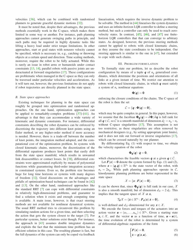
Fig. 2. Expansion of a unidirectional RRT [7].

In this system, Eq. (5) forces the states xxx to remain in X ,

and Eq. (6) models the dynamics of the robot, which can

be described using the multiplier form of the Euler-Lagrange

equations for example [48]. For each value of uuu, Eq. (6) defines

a vector field over X , which can be used together with Eq. (5)

to simulate the robot motion forward in time using proper

integration tools [49].

To model the fact that the actuator forces are limited, we

will assume that uuu can only take values inside the box

U = [−l1, l1]× [−l2, l2]× . . .× [−lnu , lnu ] (7)

of Rnu , where li denotes the limit force or torque of the i-th

motor. Along a trajectory, moreover, the robot cannot incur

in collisions with itself or with the environment, and should

fulfil any limits imposed on qqq and qqq. This reduces the feasible

states xxx to those lying in a subset Xfeas ⊆ X .

With the previous definitions, the problem we confront can

be stated as follows: Given a kinematic and dynamic model

of the robot, a geometric model of the environment, and two

states xxxs and xxxg of Xfeas, find a control policy uuu = uuu(t) lying

in U for all t such that the trajectory xxx = xxx(t) determined by

Eqs. (5) and (6) for xxx(0) = xxxs fulfils xxx(tg) = xxxg at some time

tg > 0, with xxx(t) ∈ Xfeas for all t ∈ [0, tg].

IV. LIMITATIONS OF PRIOR RRT METHODS

Observe that the previous formulation is more general than

the one assumed in earlier RRT planners. In particular, the

approaches in [10, 12, 19, 22, 23] are purely kinematic, so

they only consider Eq. (1), and neglect Eqs. (2), (6), and the

force bounds in (7). As a result, they only compute paths in C,

and such paths might be unfeasible dynamically. In contrast,

kinodynamic approaches like [7]–[9, 44, 46, 47] consider

Eq. (6) and the bounds in (7), but not Eqs. (1) and (2), which

impedes the handling of robots with closed kinematic chains.

While [24] proposed a few extensions to help RRTs cope

with such chains, we next see that these lead to unsatisfactory

results.

Recall from [24] that a usual RRT is initialised at xxxs, and

is extended by applying four steps repeatedly [see Fig. 2]: 1)

a guiding state xxxrand ∈ X is randomly selected; 2) the RRT

Rnx

X

xxxrand

xxxnear

xxx′rand

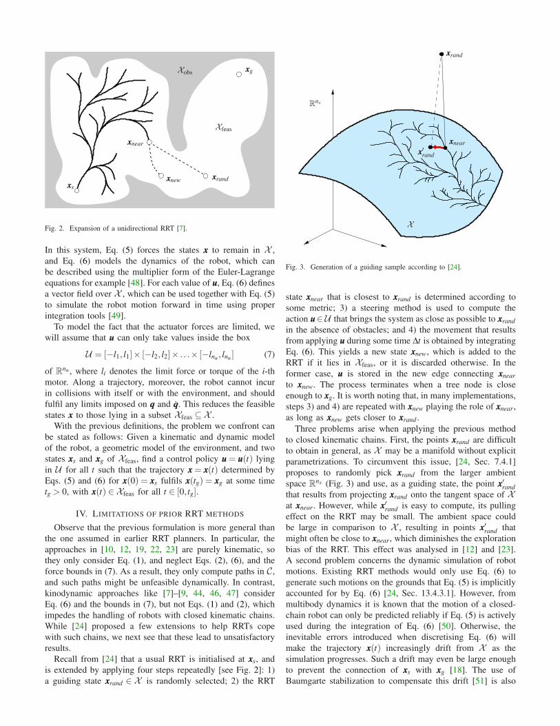
Fig. 3. Generation of a guiding sample according to [24].

state xxxnear that is closest to xxxrand is determined according to

some metric; 3) a steering method is used to compute the

action uuu∈U that brings the system as close as possible to xxxrand

in the absence of obstacles; and 4) the movement that results

from applying uuu during some time ∆t is obtained by integrating

Eq. (6). This yields a new state xxxnew, which is added to the

RRT if it lies in Xfeas, or it is discarded otherwise. In the

former case, uuu is stored in the new edge connecting xxxnear

to xxxnew. The process terminates when a tree node is close

enough to xxxg. It is worth noting that, in many implementations,

steps 3) and 4) are repeated with xxxnew playing the role of xxxnear,

as long as xxxnew gets closer to xxxrand .

Three problems arise when applying the previous method

to closed kinematic chains. First, the points xxxrand are difficult

to obtain in general, as X may be a manifold without explicit

parametrizations. To circumvent this issue, [24, Sec. 7.4.1]

proposes to randomly pick xxxrand from the larger ambient

space Rnx (Fig. 3) and use, as a guiding state, the point xxx′rand

that results from projecting xxxrand onto the tangent space of Xat xxxnear. However, while xxx′rand is easy to compute, its pulling

effect on the RRT may be small. The ambient space could

be large in comparison to X , resulting in points xxx′rand that

might often be close to xxxnear, which diminishes the exploration

bias of the RRT. This effect was analysed in [12] and [23].

A second problem concerns the dynamic simulation of robot

motions. Existing RRT methods would only use Eq. (6) to

generate such motions on the grounds that Eq. (5) is implicitly

accounted for by Eq. (6) [24, Sec. 13.4.3.1]. However, from

multibody dynamics it is known that the motion of a closed-

chain robot can only be predicted reliably if Eq. (5) is actively

used during the integration of Eq. (6) [50]. Otherwise, the

inevitable errors introduced when discretising Eq. (6) will

make the trajectory xxx(t) increasingly drift from X as the

simulation progresses. Such a drift may even be large enough

to prevent the connection of xxxs with xxxg [18]. The use of

Baumgarte stabilization to compensate this drift [51] is also

problematic, as it may lead to instabilities [52] or fictitious

energy increments, and its stabilising parameters are not easy

to tune. A third problem, finally, concerns the steering method.

A shooting strategy based on simulating random actions

from U was proposed in [7], but this technique is inefficient

when nu is large, as the number of samples needed to properly

represent U grows exponentially with nu. The lack of a good

steering strategy is a general problem of RRT methods, but it

is more difficult to address when closed kinematic chains are

present.

Purely kinematic planners like [10, 12, 19, 22, 23] do

not perform dynamic simulations, and employ direct steering

motions between configurations. Moreover, most of them

sample in ambient space. Thus, the previous three problems

would also arise when trying to generalise them to cope with

dynamic constraints. Among such planners, however, the one

in [12] is more amenable for generalisation, as it employs atlas

machinery that is applicable to mechanisms of general loop

topology. Our goal in this paper is to show that, precisely, such

a machinery can be extended to cope with the more general

problem of Section III. As we shall see, once an atlas of X is

obtained, we will have the necessary tools to 1) sample the Xmanifold directly instead of its ambient space RnX ; 2) integrate

Eqs. (5) and (6) as a true differential-algebraic equation so

as to ensure driftless motions on X ; and 3) define a proper

steering method for closed kinematic chains. We develop these

tools in the following two sections, and later use them as basic

building blocks in our planner implementation.

V. MAPPING AND EXPLORING THE STATE SPACE

A. Atlas construction

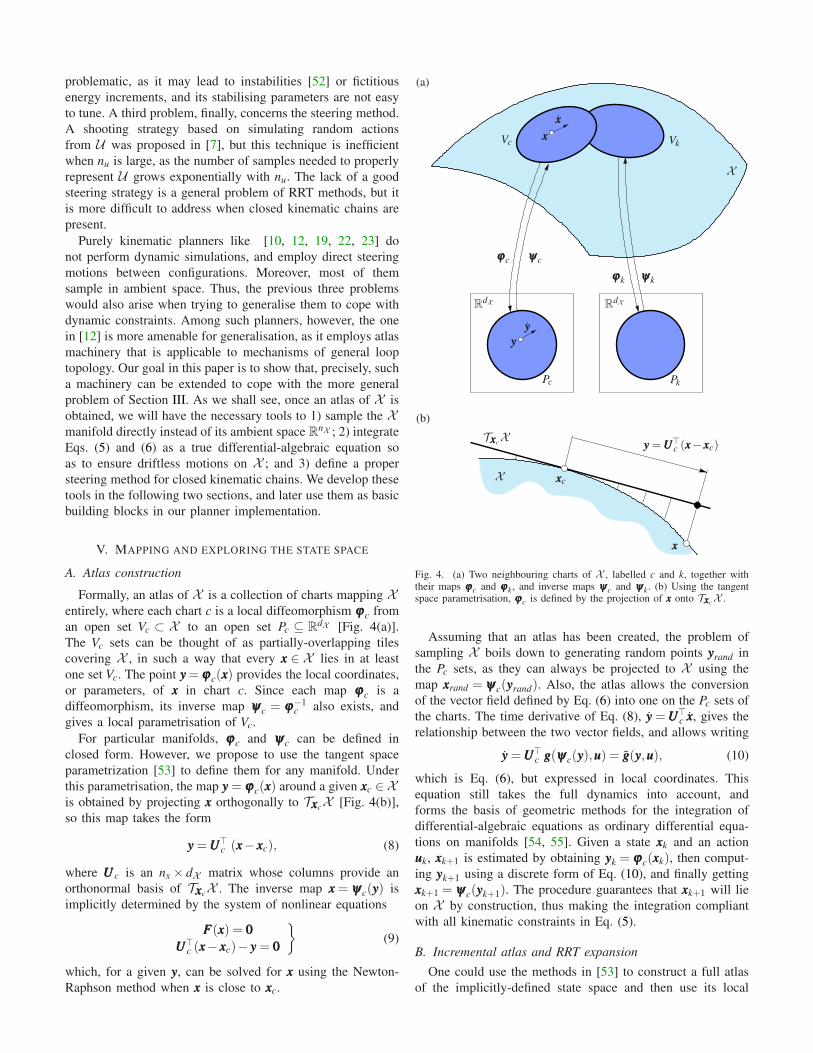
Formally, an atlas of X is a collection of charts mapping Xentirely, where each chart c is a local diffeomorphism ϕϕϕc from

an open set Vc ⊂ X to an open set Pc ⊆ RdX [Fig. 4(a)].

The Vc sets can be thought of as partially-overlapping tiles

covering X , in such a way that every xxx ∈ X lies in at least

one set Vc. The point yyy= ϕϕϕc(xxx) provides the local coordinates,

or parameters, of xxx in chart c. Since each map ϕϕϕc is a

diffeomorphism, its inverse map ψψψc = ϕϕϕ−1c also exists, and

gives a local parametrisation of Vc.

For particular manifolds, ϕϕϕc and ψψψc can be defined in

closed form. However, we propose to use the tangent space

parametrization [53] to define them for any manifold. Under

this parametrisation, the map yyy = ϕϕϕc(xxx) around a given xxxc ∈ Xis obtained by projecting xxx orthogonally to TxxxcX [Fig. 4(b)],

so this map takes the form

yyy =UUU⊤c (xxx− xxxc), (8)

where UUUc is an nx × dX matrix whose columns provide an

orthonormal basis of TxxxcX . The inverse map xxx = ψψψc(yyy) is

implicitly determined by the system of nonlinear equations

FFF(xxx) = 000

UUU⊤c (xxx− xxxc)− yyy = 000

}

(9)

which, for a given yyy, can be solved for xxx using the Newton-

Raphson method when xxx is close to xxxc.

X

X

(a)

(b)

xxx

yyy

xxx

yyy

RdXR

dX

Pc

Vc

Pk

Vk

ψψψc

ψψψk

ϕϕϕc

ϕϕϕk

xxx

TxxxcX

yyy =UUU⊤c (xxx− xxxc)

xxxc

Fig. 4. (a) Two neighbouring charts of X , labelled c and k, together withtheir maps ϕϕϕc and ϕϕϕk, and inverse maps ψψψc and ψψψk . (b) Using the tangentspace parametrisation, ϕϕϕc is defined by the projection of xxx onto TxxxcX .

Assuming that an atlas has been created, the problem of

sampling X boils down to generating random points yyyrand in

the Pc sets, as they can always be projected to X using the

map xxxrand = ψψψc(yyyrand). Also, the atlas allows the conversion

of the vector field defined by Eq. (6) into one on the Pc sets of

the charts. The time derivative of Eq. (8), yyy =UUU⊤c xxx, gives the

relationship between the two vector fields, and allows writing

yyy =UUU⊤c ggg(ψψψc(yyy),uuu) = ggg(yyy,uuu), (10)

which is Eq. (6), but expressed in local coordinates. This

equation still takes the full dynamics into account, and

forms the basis of geometric methods for the integration of

differential-algebraic equations as ordinary differential equa-

tions on manifolds [54, 55]. Given a state xxxk and an action

uuuk, xxxk+1 is estimated by obtaining yyyk = ϕϕϕc(xxxk), then comput-

ing yyyk+1 using a discrete form of Eq. (10), and finally getting

xxxk+1 = ψψψc(yyyk+1). The procedure guarantees that xxxk+1 will lie

on X by construction, thus making the integration compliant

with all kinematic constraints in Eq. (5).

B. Incremental atlas and RRT expansion

One could use the methods in [53] to construct a full atlas

of the implicitly-defined state space and then use its local

xxxc

xxxk

xxxk+1

yyyk yyyk+1

α

ε

ρ

TxxxcX

X

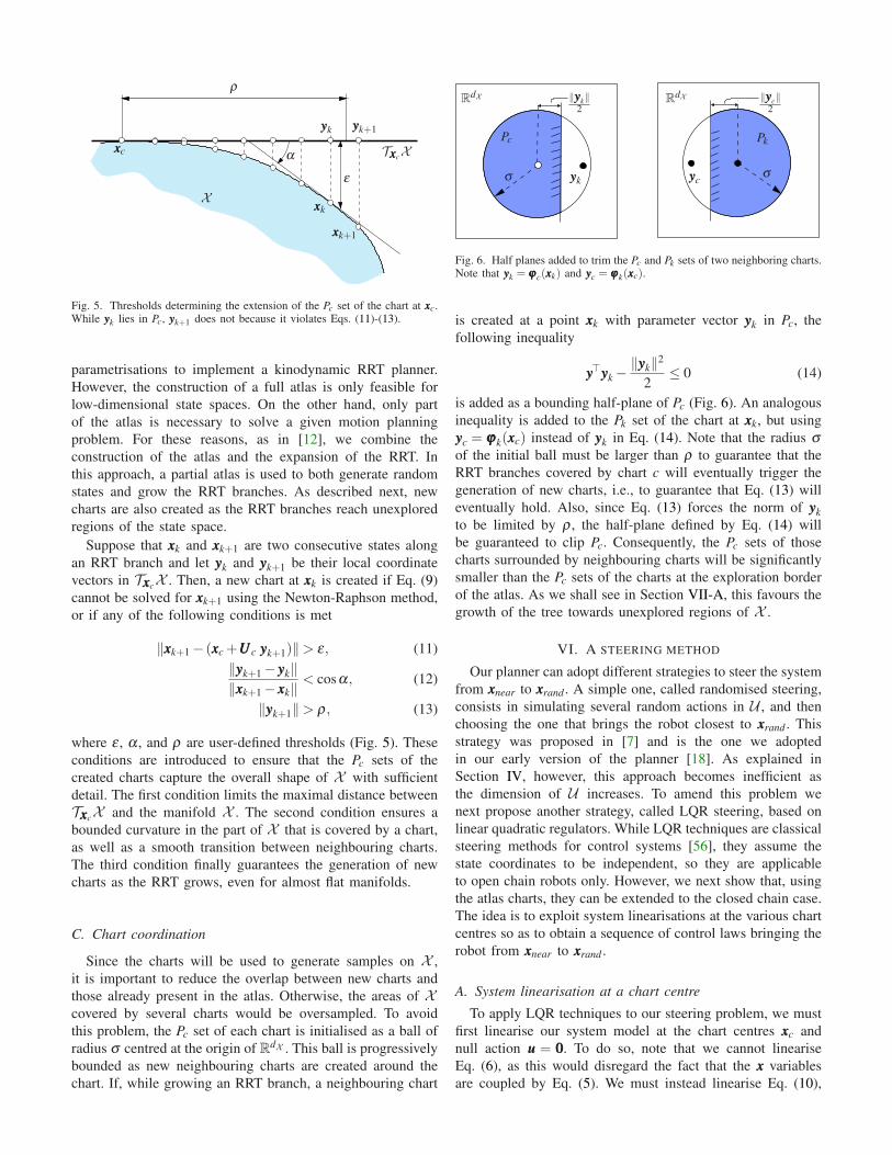
Fig. 5. Thresholds determining the extension of the Pc set of the chart at xxxc.While yyyk lies in Pc, yyyk+1 does not because it violates Eqs. (11)-(13).

parametrisations to implement a kinodynamic RRT planner.

However, the construction of a full atlas is only feasible for

low-dimensional state spaces. On the other hand, only part

of the atlas is necessary to solve a given motion planning

problem. For these reasons, as in [12], we combine the

construction of the atlas and the expansion of the RRT. In

this approach, a partial atlas is used to both generate random

states and grow the RRT branches. As described next, new

charts are also created as the RRT branches reach unexplored

regions of the state space.

Suppose that xxxk and xxxk+1 are two consecutive states along

an RRT branch and let yyyk and yyyk+1 be their local coordinate

vectors in TxxxcX . Then, a new chart at xxxk is created if Eq. (9)

cannot be solved for xxxk+1 using the Newton-Raphson method,

or if any of the following conditions is met

‖xxxk+1− (xxxc +UUUc yyyk+1)‖> ε , (11)

‖yyyk+1− yyyk‖‖xxxk+1− xxxk‖

< cosα, (12)

‖yyyk+1‖> ρ , (13)

where ε , α , and ρ are user-defined thresholds (Fig. 5). These

conditions are introduced to ensure that the Pc sets of the

created charts capture the overall shape of X with sufficient

detail. The first condition limits the maximal distance between

TxxxcX and the manifold X . The second condition ensures a

bounded curvature in the part of X that is covered by a chart,

as well as a smooth transition between neighbouring charts.

The third condition finally guarantees the generation of new

charts as the RRT grows, even for almost flat manifolds.

C. Chart coordination

Since the charts will be used to generate samples on X ,

it is important to reduce the overlap between new charts and

those already present in the atlas. Otherwise, the areas of Xcovered by several charts would be oversampled. To avoid

this problem, the Pc set of each chart is initialised as a ball of

radius σ centred at the origin of RdX . This ball is progressively

bounded as new neighbouring charts are created around the

chart. If, while growing an RRT branch, a neighbouring chart

‖yyyk‖2

‖yyyc‖2

σσ yyyk yyyc

RdXR

dX

Pc Pk

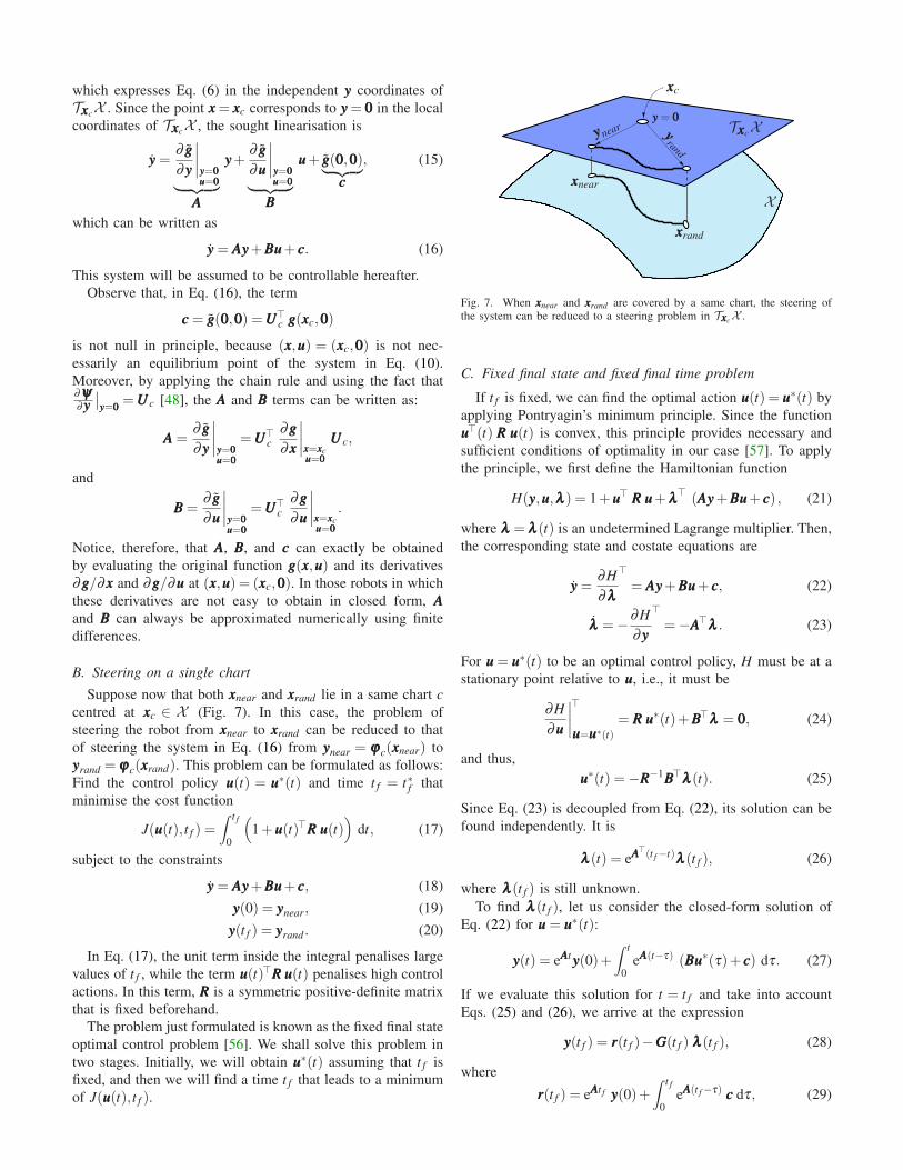
Fig. 6. Half planes added to trim the Pc and Pk sets of two neighboring charts.Note that yyyk = ϕϕϕc(xxxk) and yyyc = ϕϕϕk(xxxc).

is created at a point xxxk with parameter vector yyyk in Pc, the

following inequality

yyy⊤yyyk−‖yyyk‖2

2≤ 0 (14)

is added as a bounding half-plane of Pc (Fig. 6). An analogous

inequality is added to the Pk set of the chart at xxxk, but using

yyyc = ϕϕϕk(xxxc) instead of yyyk in Eq. (14). Note that the radius σof the initial ball must be larger than ρ to guarantee that the

RRT branches covered by chart c will eventually trigger the

generation of new charts, i.e., to guarantee that Eq. (13) will

eventually hold. Also, since Eq. (13) forces the norm of yyyk

to be limited by ρ , the half-plane defined by Eq. (14) will

be guaranteed to clip Pc. Consequently, the Pc sets of those

charts surrounded by neighbouring charts will be significantly

smaller than the Pc sets of the charts at the exploration border

of the atlas. As we shall see in Section VII-A, this favours the

growth of the tree towards unexplored regions of X .

VI. A STEERING METHOD

Our planner can adopt different strategies to steer the system

from xxxnear to xxxrand . A simple one, called randomised steering,

consists in simulating several random actions in U , and then

choosing the one that brings the robot closest to xxxrand . This

strategy was proposed in [7] and is the one we adopted

in our early version of the planner [18]. As explained in

Section IV, however, this approach becomes inefficient as

the dimension of U increases. To amend this problem we

next propose another strategy, called LQR steering, based on

linear quadratic regulators. While LQR techniques are classical

steering methods for control systems [56], they assume the

state coordinates to be independent, so they are applicable

to open chain robots only. However, we next show that, using

the atlas charts, they can be extended to the closed chain case.

The idea is to exploit system linearisations at the various chart

centres so as to obtain a sequence of control laws bringing the

robot from xxxnear to xxxrand .

A. System linearisation at a chart centre

To apply LQR techniques to our steering problem, we must

first linearise our system model at the chart centres xxxc and

null action uuu = 000. To do so, note that we cannot linearise

Eq. (6), as this would disregard the fact that the xxx variables

are coupled by Eq. (5). We must instead linearise Eq. (10),

which expresses Eq. (6) in the independent yyy coordinates of

TxxxcX . Since the point xxx = xxxc corresponds to yyy = 000 in the local

coordinates of TxxxcX , the sought linearisation is

yyy =∂ ggg

∂yyy

∣∣∣∣

yyy=000uuu=000

︸ ︷︷ ︸

AAA

yyy+∂ ggg

∂uuu

∣∣∣∣

yyy=000uuu=000

︸ ︷︷ ︸

BBB

uuu+ ggg(000,000)︸ ︷︷ ︸

ccc

, (15)

which can be written as

yyy = AAAyyy+BBBuuu+ ccc. (16)

This system will be assumed to be controllable hereafter.

Observe that, in Eq. (16), the term

ccc = ggg(000,000) =UUU⊤c ggg(xxxc,000)

is not null in principle, because (xxx,uuu) = (xxxc,000) is not nec-

essarily an equilibrium point of the system in Eq. (10).

Moreover, by applying the chain rule and using the fact that∂ψψψ∂yyy

∣∣yyy=000

=UUUc [48], the AAA and BBB terms can be written as:

AAA =∂ ggg

∂yyy

∣∣∣∣

yyy=000uuu=000

=UUU⊤c∂ggg

∂xxx

∣∣∣∣xxx=xxxc

uuu=000

UUUc,

and

BBB =∂ ggg

∂uuu

∣∣∣∣

yyy=000uuu=000

=UUU⊤c∂ggg

∂uuu

∣∣∣∣xxx=xxxc

uuu=000

.

Notice, therefore, that AAA, BBB, and ccc can exactly be obtained

by evaluating the original function ggg(xxx,uuu) and its derivatives

∂ggg/∂xxx and ∂ggg/∂uuu at (xxx,uuu) = (xxxc,000). In those robots in which

these derivatives are not easy to obtain in closed form, AAA

and BBB can always be approximated numerically using finite

differences.

B. Steering on a single chart

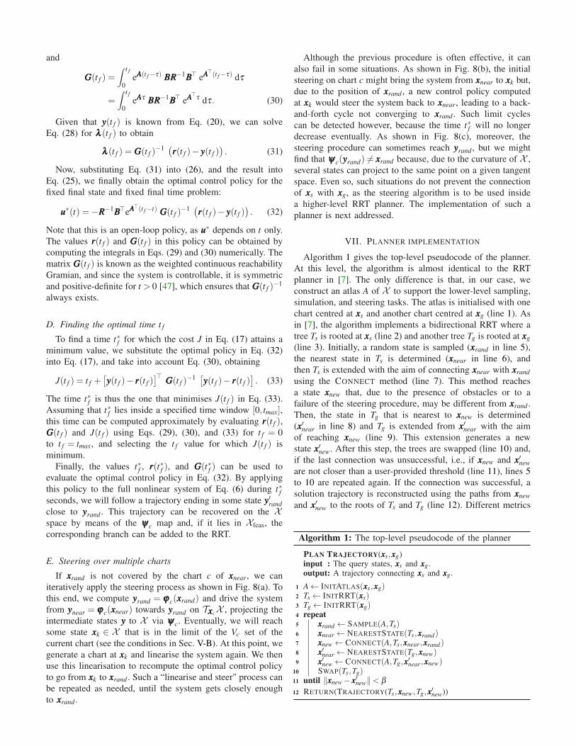
Suppose now that both xxxnear and xxxrand lie in a same chart c

centred at xxxc ∈ X (Fig. 7). In this case, the problem of

steering the robot from xxxnear to xxxrand can be reduced to that

of steering the system in Eq. (16) from yyynear = ϕϕϕc(xxxnear) to

yyyrand = ϕϕϕc(xxxrand). This problem can be formulated as follows:

Find the control policy uuu(t) = uuu∗(t) and time t f = t∗f that

minimise the cost function

J(uuu(t), t f ) =∫ t f

0

(

1+uuu(t)⊤RRR uuu(t))

dt, (17)

subject to the constraints

yyy = AAAyyy+BBBuuu+ ccc, (18)

yyy(0) = yyynear, (19)

yyy(t f ) = yyyrand . (20)

In Eq. (17), the unit term inside the integral penalises large

values of t f , while the term uuu(t)⊤RRR uuu(t) penalises high control

actions. In this term, RRR is a symmetric positive-definite matrix

that is fixed beforehand.

The problem just formulated is known as the fixed final state

optimal control problem [56]. We shall solve this problem in

two stages. Initially, we will obtain uuu∗(t) assuming that t f is

fixed, and then we will find a time t f that leads to a minimum

of J(uuu(t), t f ).

X

xxxrand

xxxnear

xxxc

yyy = 000

yyyrand

yyy near TxxxcX

Fig. 7. When xxxnear and xxxrand are covered by a same chart, the steering ofthe system can be reduced to a steering problem in TxxxcX .

C. Fixed final state and fixed final time problem

If t f is fixed, we can find the optimal action uuu(t) = uuu∗(t) by

applying Pontryagin’s minimum principle. Since the function

uuu⊤(t) RRR uuu(t) is convex, this principle provides necessary and

sufficient conditions of optimality in our case [57]. To apply

the principle, we first define the Hamiltonian function

H(yyy,uuu,λλλ ) = 1+uuu⊤ RRR uuu+λλλ⊤ (AAAyyy+BBBuuu+ ccc) , (21)

where λλλ = λλλ (t) is an undetermined Lagrange multiplier. Then,

the corresponding state and costate equations are

yyy =∂H

∂λλλ

⊤= AAAyyy+BBBuuu+ ccc, (22)

λλλ =−∂H

∂yyy

⊤=−AAA⊤λλλ . (23)

For uuu = uuu∗(t) to be an optimal control policy, H must be at a

stationary point relative to uuu, i.e., it must be

∂H

∂uuu

∣∣∣∣

⊤

uuu=uuu∗(t)= RRR uuu∗(t)+BBB⊤λλλ = 000, (24)

and thus,

uuu∗(t) =−RRR−1BBB⊤λλλ (t). (25)

Since Eq. (23) is decoupled from Eq. (22), its solution can be

found independently. It is

λλλ (t) = eAAA⊤(t f−t)λλλ (t f ), (26)

where λλλ (t f ) is still unknown.

To find λλλ (t f ), let us consider the closed-form solution of

Eq. (22) for uuu = uuu∗(t):

yyy(t) = eAAAtyyy(0)+∫ t

0eAAA(t−τ) (BBBuuu∗(τ)+ ccc) dτ . (27)

If we evaluate this solution for t = t f and take into account

Eqs. (25) and (26), we arrive at the expression

yyy(t f ) = rrr(t f )−GGG(t f ) λλλ (t f ), (28)

where

rrr(t f ) = eAAAt f yyy(0)+∫ t f

0eAAA(t f−τ) ccc dτ , (29)

and

GGG(t f ) =∫ t f

0eAAA(t f−τ) BBBRRR−1BBB⊤ eAAA⊤(t f−τ) dτ

=∫ t f

0eAAAτ BBBRRR−1BBB⊤ eAAA⊤τ dτ . (30)

Given that yyy(t f ) is known from Eq. (20), we can solve

Eq. (28) for λλλ (t f ) to obtain

λλλ (t f ) = GGG(t f )−1

(rrr(t f )− yyy(t f )

). (31)

Now, substituting Eq. (31) into (26), and the result into

Eq. (25), we finally obtain the optimal control policy for the

fixed final state and fixed final time problem:

uuu∗(t) =−RRR−1BBB⊤eAAA⊤(t f−t) GGG(t f )−1

(rrr(t f )− yyy(t f )

). (32)

Note that this is an open-loop policy, as uuu∗ depends on t only.

The values rrr(t f ) and GGG(t f ) in this policy can be obtained by

computing the integrals in Eqs. (29) and (30) numerically. The

matrix GGG(t f ) is known as the weighted continuous reachability

Gramian, and since the system is controllable, it is symmetric

and positive-definite for t > 0 [47], which ensures that GGG(t f )−1

always exists.

D. Finding the optimal time t f

To find a time t∗f for which the cost J in Eq. (17) attains a

minimum value, we substitute the optimal policy in Eq. (32)

into Eq. (17), and take into account Eq. (30), obtaining

J(t f ) = t f +[yyy(t f )− rrr(t f )

]⊤GGG(t f )

−1[yyy(t f )− rrr(t f )

]. (33)

The time t∗f is thus the one that minimises J(t f ) in Eq. (33).

Assuming that t∗f lies inside a specified time window [0, tmax],this time can be computed approximately by evaluating rrr(t f ),GGG(t f ) and J(t f ) using Eqs. (29), (30), and (33) for t f = 0

to t f = tmax, and selecting the t f value for which J(t f ) is

minimum.

Finally, the values t∗f , rrr(t∗f ), and GGG(t∗f ) can be used to

evaluate the optimal control policy in Eq. (32). By applying

this policy to the full nonlinear system of Eq. (6) during t∗fseconds, we will follow a trajectory ending in some state yyy′rand

close to yyyrand . This trajectory can be recovered on the Xspace by means of the ψψψc map and, if it lies in Xfeas, the

corresponding branch can be added to the RRT.

E. Steering over multiple charts

If xxxrand is not covered by the chart c of xxxnear, we can

iteratively apply the steering process as shown in Fig. 8(a). To

this end, we compute yyyrand = ϕϕϕc(xxxrand) and drive the system

from yyynear = ϕϕϕc(xxxnear) towards yyyrand on TxxxcX , projecting the

intermediate states yyy to X via ψψψc. Eventually, we will reach

some state xxxk ∈ X that is in the limit of the Vc set of the

current chart (see the conditions in Sec. V-B). At this point, we

generate a chart at xxxk and linearise the system again. We then

use this linearisation to recompute the optimal control policy

to go from xxxk to xxxrand . Such a “linearise and steer" process can

be repeated as needed, until the system gets closely enough

to xxxrand .

Although the previous procedure is often effective, it can

also fail in some situations. As shown in Fig. 8(b), the initial

steering on chart c might bring the system from xxxnear to xxxk but,

due to the position of xxxrand , a new control policy computed

at xxxk would steer the system back to xxxnear, leading to a back-

and-forth cycle not converging to xxxrand . Such limit cycles

can be detected however, because the time t∗f will no longer

decrease eventually. As shown in Fig. 8(c), moreover, the

steering procedure can sometimes reach yyyrand , but we might

find that ψψψc(yyyrand) 6= xxxrand because, due to the curvature of X ,

several states can project to the same point on a given tangent

space. Even so, such situations do not prevent the connection

of xxxs with xxxg, as the steering algorithm is to be used inside

a higher-level RRT planner. The implementation of such a

planner is next addressed.

VII. PLANNER IMPLEMENTATION

Algorithm 1 gives the top-level pseudocode of the planner.

At this level, the algorithm is almost identical to the RRT

planner in [7]. The only difference is that, in our case, we

construct an atlas A of X to support the lower-level sampling,

simulation, and steering tasks. The atlas is initialised with one

chart centred at xxxs and another chart centred at xxxg (line 1). As

in [7], the algorithm implements a bidirectional RRT where a

tree Ts is rooted at xxxs (line 2) and another tree Tg is rooted at xxxg

(line 3). Initially, a random state is sampled (xxxrand in line 5),

the nearest state in Ts is determined (xxxnear in line 6), and

then Ts is extended with the aim of connecting xxxnear with xxxrand

using the CONNECT method (line 7). This method reaches

a state xxxnew that, due to the presence of obstacles or to a

failure of the steering procedure, may be different from xxxrand .

Then, the state in Tg that is nearest to xxxnew is determined

(xxx′near in line 8) and Tg is extended from xxx′near with the aim

of reaching xxxnew (line 9). This extension generates a new

state xxx′new. After this step, the trees are swapped (line 10) and,

if the last connection was unsuccessful, i.e., if xxxnew and xxx′new

are not closer than a user-provided threshold (line 11), lines 5

to 10 are repeated again. If the connection was successful, a

solution trajectory is reconstructed using the paths from xxxnew

and xxx′new to the roots of Ts and Tg (line 12). Different metrics

Algorithm 1: The top-level pseudocode of the planner

PLAN TRAJECTORY(xxxs,xxxg)input : The query states, xxxs and xxxg.output: A trajectory connecting xxxs and xxxg.

1 A← INITATLAS(xxxs,xxxg)2 Ts← INITRRT(xxxs)3 Tg← INITRRT(xxxg)4 repeat5 xxxrand ← SAMPLE(A,Ts)6 xxxnear← NEARESTSTATE(Ts,xxxrand)7 xxxnew← CONNECT(A,Ts,xxxnear,xxxrand)8 xxx′near← NEARESTSTATE(Tg,xxxnew)9 xxx′new← CONNECT(A,Tg,xxx

′near,xxxnew)

10 SWAP(Ts,Tg)11 until ‖xxxnew− xxx′new‖< β

12 RETURN(TRAJECTORY(Ts,xxxnew,Tg,xxx′new))

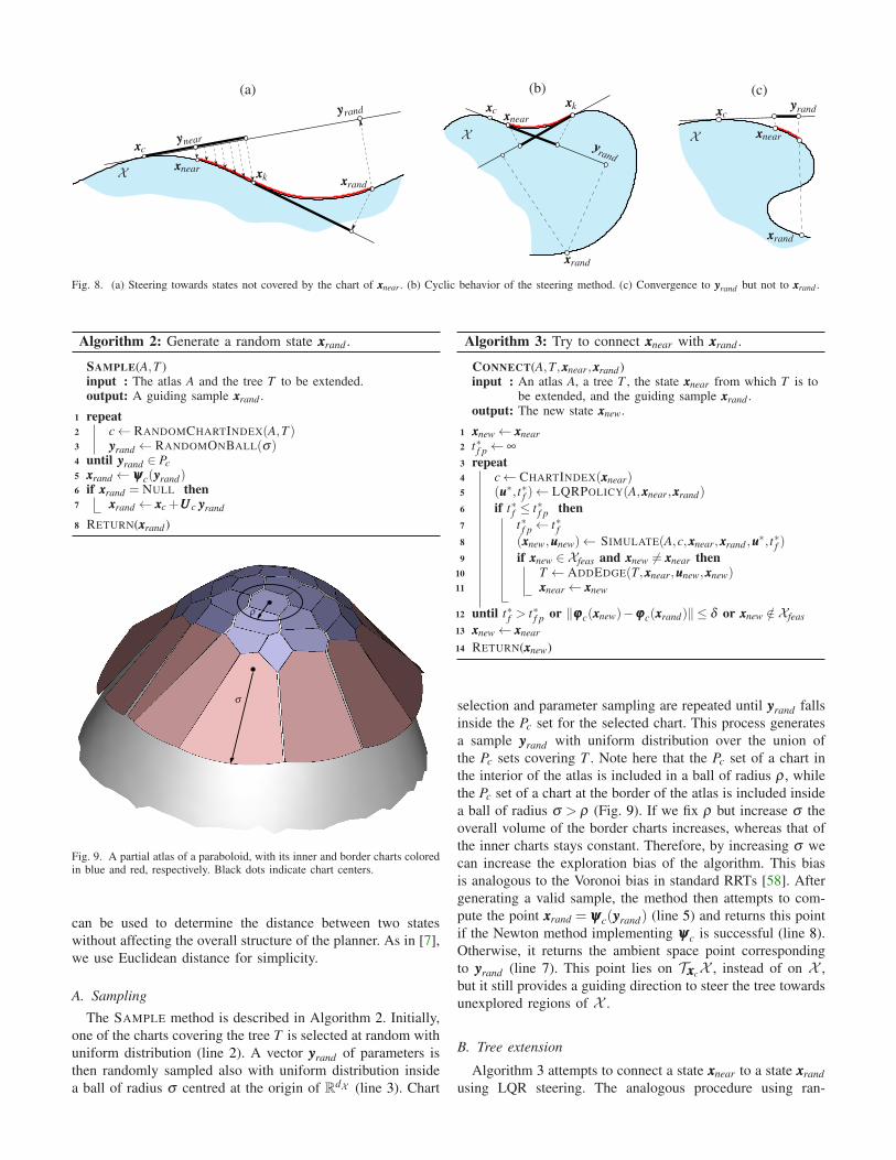
(a) (b) (c)

xxxnear

xxxnear

xxxnear

yyynear X X

X

xxxrand

xxxrand

xxxrand

yyyrandyyyrand

yyyrand

xxxk

xxxk

xxxc

xxxcxxxc

Fig. 8. (a) Steering towards states not covered by the chart of xxxnear . (b) Cyclic behavior of the steering method. (c) Convergence to yyyrand but not to xxxrand .

Algorithm 2: Generate a random state xxxrand .

SAMPLE(A,T )input : The atlas A and the tree T to be extended.output: A guiding sample xxxrand .

1 repeat2 c← RANDOMCHARTINDEX(A,T )3 yyyrand ← RANDOMONBALL(σ)4 until yyyrand ∈ Pc

5 xxxrand ← ψψψc(yyyrand)6 if xxxrand = NULL then7 xxxrand ← xxxc +UUUc yyyrand

8 RETURN(xxxrand)

σ

ρ

Fig. 9. A partial atlas of a paraboloid, with its inner and border charts coloredin blue and red, respectively. Black dots indicate chart centers.

can be used to determine the distance between two states

without affecting the overall structure of the planner. As in [7],

we use Euclidean distance for simplicity.

A. Sampling

The SAMPLE method is described in Algorithm 2. Initially,

one of the charts covering the tree T is selected at random with

uniform distribution (line 2). A vector yyyrand of parameters is

then randomly sampled also with uniform distribution inside

a ball of radius σ centred at the origin of RdX (line 3). Chart

Algorithm 3: Try to connect xxxnear with xxxrand .

CONNECT(A,T,xxxnear,xxxrand)input : An atlas A, a tree T , the state xxxnear from which T is to

be extended, and the guiding sample xxxrand .output: The new state xxxnew.

1 xxxnew← xxxnear

2 t∗f p← ∞

3 repeat4 c← CHARTINDEX(xxxnear)5 (uuu∗, t∗f )← LQRPOLICY(A,xxxnear,xxxrand)

6 if t∗f ≤ t∗f p then

7 t∗f p← t∗f8 (xxxnew,uuunew)← SIMULATE(A,c,xxxnear,xxxrand ,uuu

∗, t∗f )9 if xxxnew ∈ Xfeas and xxxnew 6= xxxnear then

10 T ← ADDEDGE(T,xxxnear,uuunew,xxxnew)11 xxxnear← xxxnew

12 until t∗f > t∗f p or ‖ϕϕϕc(xxxnew)−ϕϕϕc(xxxrand)‖ ≤ δ or xxxnew /∈ Xfeas

13 xxxnew← xxxnear

14 RETURN(xxxnew)

selection and parameter sampling are repeated until yyyrand falls

inside the Pc set for the selected chart. This process generates

a sample yyyrand with uniform distribution over the union of

the Pc sets covering T . Note here that the Pc set of a chart in

the interior of the atlas is included in a ball of radius ρ , while

the Pc set of a chart at the border of the atlas is included inside

a ball of radius σ > ρ (Fig. 9). If we fix ρ but increase σ the

overall volume of the border charts increases, whereas that of

the inner charts stays constant. Therefore, by increasing σ we

can increase the exploration bias of the algorithm. This bias

is analogous to the Voronoi bias in standard RRTs [58]. After

generating a valid sample, the method then attempts to com-

pute the point xxxrand = ψψψc(yyyrand) (line 5) and returns this point

if the Newton method implementing ψψψc is successful (line 8).

Otherwise, it returns the ambient space point corresponding

to yyyrand (line 7). This point lies on TxxxcX , instead of on X ,

but it still provides a guiding direction to steer the tree towards

unexplored regions of X .

B. Tree extension

Algorithm 3 attempts to connect a state xxxnear to a state xxxrand

using LQR steering. The analogous procedure using ran-

Algorithm 4: Simulate an action.

SIMULATE(A,c,xxxk,xxxrand ,uuu∗, t∗f )

input : An atlas, A, the chart index c, the state from where tostart the simulation, xxxk, the state to approach, xxxrand ,the policy to simulate, uuu∗, and the optimal time t∗f to

simulate.output: The last state in the simulation and the executed

control sequence.

1 t← 02 uuuk← /03 VALIDSTATE← TRUE

4 while VALIDSTATE and ‖ϕϕϕc(xxxk)−ϕϕϕc(xxxrand)‖> δ and |t|< t∗fdo

5 (xxxk+1,yyyk+1,h)← NEXTSTATE(xxxk,yyyk,uuu∗(t),FFF,xxxc,UUUc,δ )

6 if xxxk+1 /∈ Xfeas then7 xxxk← xxxk+1

8 VALIDSTATE← FALSE

9 else10 if ‖xxxk+1− (xxxc +UUUc yyyk+1)‖> ε or11 ‖yyyk+1− yyyk‖/‖xxxk+1− xxxk‖< cos(α) or12 ‖yyyk+1‖> ρ then13 ADDCHARTTOATLAS(A,xxxk)14 VALIDSTATE← FALSE

15 else16 xxxk← xxxk+1

17 uuuk← uuuk ∪{(uuu(t),h)}18 t← t +h19 if yyyk+1 /∈ Pc then20 VALIDSTATE← FALSE

21 RETURN(xxxk,uuuk)

domised steering is available in [18]. The algorithm imple-

ments a loop where, initially, the optimal policy uuu∗ and time

t∗f to connect these two states are computed (line 5). The policy

is a function of time given by Eq. (32). If t∗f is lower than the

optimal time t∗f p obtained in the previous iteration, the policy is

used to simulate the evolution of the system from xxxnear (line 8).

The simulation produces a state xxxnew which, if it is feasible

and different from xxxnear, it is added to the tree. This involves

the creation of an edge between xxxnear and xxxnew (line 10), which

stores the control sequence uuunew executed in the simulation.

The loop is repeated until t∗f is larger than t∗f p (line 12), or xxxrand

is reached with accuracy δ in parameter space, or the next state

is unfeasible.

Algorithm 4 summarises the procedure used to simulate a

given policy uuu∗(t) from a particular state xxxk. The simulation

progresses while the new state is valid, the target state is

not reached with accuracy δ in parameter space, and the

integration time t is lower than t∗f (line 4). A state is not valid if

is not in Xfeas (line 8), if it is not in the validity area of the chart

(line 14), or if it is not included in the current Pc set (line 20),

i.e., it is parametrised by a neighbouring chart. In the first

case, both the simulation and the connection between states

are stopped. In the last two cases the simulation is stopped, but

the connection continues after recomputing the optimal policy,

on a newly created chart (line 13) or on the neighbouring chart,

respectively.

The key procedure in the simulation is the NEXTSTATE

method (line 5), which provides the next state xxxk+1, given the

current state xxxk and the action uuu∗(t) at time t. The elements

of uuu∗(t) are saturated to their bounds in Eq. (7) if such

bounds are surpassed. Then, the simulation is implemented

by integrating Eq. (6) using local coordinates as explained in

Section V-A. Any numerical integration method, either explicit

or implicit, could be used to discretise Eq. (10). We here apply

the trapezoidal rule as it yields an implicit integrator whose

computational cost (integration and projection to the manifold)

is similar to the cost of using an explicit method of the same

order [49]. Using this rule, Eq. (10) is discretised as

yyyk+1 = yyyk +h

2UUU⊤c (ggg(xxxk,uuu)+ggg(xxxk+1,uuu)), (34)

where h is the integration time step. The value xxxk+1 in Eq. (34)

is unknown but, since it must satisfy Eq. (9), it must fulfil

FFF(xxxk+1) = 000,

UUU⊤c (xxxk+1− xxxc)− yyyk+1 = 000.(35)

Now, substituting Eqs. (34) into Eq. (35) we obtain

FFF(xxxk+1) = 000,

UUU⊤c (xxxk+1− h2(ggg(xxxk,uuu)+ggg(xxxk+1,uuu))− xxxc)− yyyk = 000,

(36)

where xxxk, yyyk, and xxxc are known and xxxk+1 is the unknown

to be determined. We could use a Newton method to solve

this system, but the Broyden method is preferable as it avoids

the computation of the Jacobian of the system at each step.

Potra and Yen [49] gave an approximation of this Jacobian

that allows finding xxxk+1 in only a few iterations. For backward

integration, i.e., when extending the RRT with root at xxxg, the

time step h in Eq. (36) must simply be negative.

C. Setting the planner parameters

The planner depends on eight parameters: the three param-

eters ε , α , and ρ controlling chart creation, the radius σ used

for sampling, the tolerances δ and β measuring closeness

between states and trees, respectively, and the LQR steering

parameters RRR and tmax. All of them are positive reals except RRR,

which must be a nu×nu symmetric positive-definite matrix.

Parameters ε , α , and ρ appear, respectively, in Eqs. (11),

(12), and (13). Parameter α bounds the angle between neigh-

boring charts. This angle should be small, otherwise the Vc sets

for neighboring charts might not overlap, impeding a smooth

transition between the charts [53]. Such problematic areas can

be detected and patched [12], but this process introduces inef-

ficiencies. Thus, we suggest to keep this parameter below π/6.

Parameter ε is only relevant if the distance between the mani-

fold and the tangent space becomes large without a significant

change in curvature, which rarely occurs. Since this distance is

computed in ambient space, if on average we wish to tolerate

an error of e in each dimension, we should set ε ≃ e√

nX .

In our test cases we have used ε = 0.05√

nX . Finally, ρonly plays a relevant role on almost flat manifolds. The only

restriction to consider is that ρ must be smaller than σ to

ensure the eventual creation of new charts. Following [12], we

suggest to set ρ = dX /2. With this value, charts are generally

created before the numerical process implementing Eq. (9)

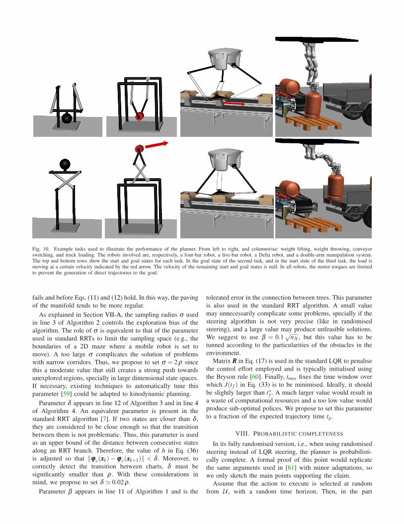
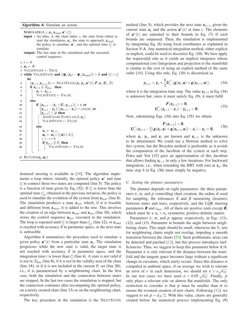
Fig. 10. Example tasks used to illustrate the performance of the planner. From left to right, and columnwise: weight lifting, weight throwing, conveyorswitching, and truck loading. The robots involved are, respectively, a four-bar robot, a five-bar robot, a Delta robot, and a double-arm manipulation system.The top and bottom rows show the start and goal states for each task. In the goal state of the second task, and in the start state of the third task, the load ismoving at a certain velocity indicated by the red arrow. The velocity of the remaining start and goal states is null. In all robots, the motor torques are limitedto prevent the generation of direct trajectories to the goal.

fails and before Eqs. (11) and (12) hold. In this way, the paving

of the manifold tends to be more regular.

As explained in Section VII-A, the sampling radius σ used

in line 3 of Algorithm 2 controls the exploration bias of the

algorithm. The role of σ is equivalent to that of the parameter

used in standard RRTs to limit the sampling space (e.g., the

boundaries of a 2D maze where a mobile robot is set to

move). A too large σ complicates the solution of problems

with narrow corridors. Thus, we propose to set σ = 2 ρ since

this a moderate value that still creates a strong push towards

unexplored regions, specially in large dimensional state spaces.

If necessary, existing techniques to automatically tune this

parameter [59] could be adapted to kinodynamic planning.

Parameter δ appears in line 12 of Algorithm 3 and in line 4

of Algorithm 4. An equivalent parameter is present in the

standard RRT algorithm [7]. If two states are closer than δ ,

they are considered to be close enough so that the transition

between them is not problematic. Thus, this parameter is used

as an upper bound of the distance between consecutive states

along an RRT branch. Therefore, the value of h in Eq. (36)

is adjusted so that ‖ϕϕϕc(xxxk)− ϕϕϕc(xxxk+1)‖ < δ . Moreover, to

correctly detect the transition between charts, δ must be

significantly smaller than ρ . With these considerations in

mind, we propose to set δ ≃ 0.02 ρ .

Parameter β appears in line 11 of Algorithm 1 and is the

tolerated error in the connection between trees. This parameter

is also used in the standard RRT algorithm. A small value

may unnecessarily complicate some problems, specially if the

steering algorithm is not very precise (like in randomised

steering), and a large value may produce unfeasible solutions.

We suggest to use β = 0.1√

nX , but this value has to be

tunned according to the particularities of the obstacles in the

environment.

Matrix RRR in Eq. (17) is used in the standard LQR to penalise

the control effort employed and is typically initialised using

the Bryson rule [60]. Finally, tmax fixes the time window over

which J(t f ) in Eq. (33) is to be minimised. Ideally, it should

be slightly larger than t∗f . A much larger value would result in

a waste of computational resources and a too low value would

produce sub-optimal polices. We propose to set this parameter

to a fraction of the expected trajectory time tg.

VIII. PROBABILISTIC COMPLETENESS

In its fully randomised version, i.e., when using randomised

steering instead of LQR steering, the planner is probabilisti-

cally complete. A formal proof of this point would replicate

the same arguments used in [61] with minor adaptations, so

we only sketch the main points supporting the claim.

Assume that the action to execute is selected at random

from U , with a random time horizon. Then, in the part

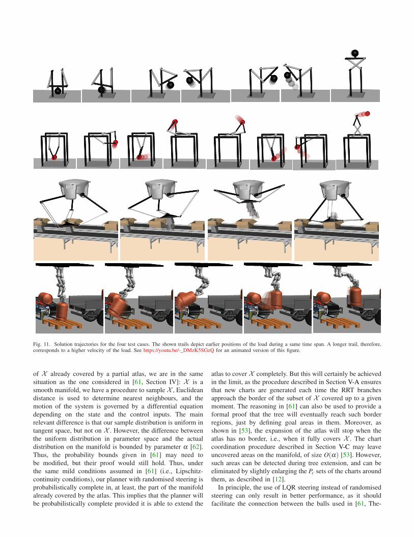
Fig. 11. Solution trajectories for the four test cases. The shown trails depict earlier positions of the load during a same time span. A longer trail, therefore,corresponds to a higher velocity of the load. See https://youtu.be/-_DMzK5SGzQ for an animated version of this figure.

of X already covered by a partial atlas, we are in the same

situation as the one considered in [61, Section IV]: X is a

smooth manifold, we have a procedure to sample X , Euclidean

distance is used to determine nearest neighbours, and the

motion of the system is governed by a differential equation

depending on the state and the control inputs. The main

relevant difference is that our sample distribution is uniform in

tangent space, but not on X . However, the difference between

the uniform distribution in parameter space and the actual

distribution on the manifold is bounded by parameter α [62].

Thus, the probability bounds given in [61] may need to

be modified, but their proof would still hold. Thus, under

the same mild conditions assumed in [61] (i.e., Lipschitz-

continuity conditions), our planner with randomised steering is

probabilistically complete in, at least, the part of the manifold

already covered by the atlas. This implies that the planner will

be probabilistically complete provided it is able to extend the

atlas to cover X completely. But this will certainly be achieved

in the limit, as the procedure described in Section V-A ensures

that new charts are generated each time the RRT branches

approach the border of the subset of X covered up to a given

moment. The reasoning in [61] can also be used to provide a

formal proof that the tree will eventually reach such border

regions, just by defining goal areas in them. Moreover, as

shown in [53], the expansion of the atlas will stop when the

atlas has no border, i.e., when it fully covers X . The chart

coordination procedure described in Section V-C may leave

uncovered areas on the manifold, of size O(α) [53]. However,

such areas can be detected during tree extension, and can be

eliminated by slightly enlarging the Pc sets of the charts around

them, as described in [12].

In principle, the use of LQR steering instead of randomised

steering can only result in better performance, as it should

facilitate the connection between the balls used in [61, The-

q1

q2

q3

q4

x0

x1

x2

x3

L0

L1

L2

L3

J1

J2J3

J4

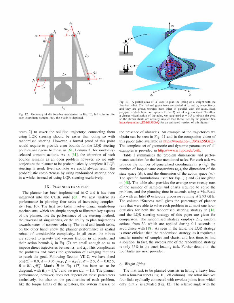
Fig. 12. Geometry of the four-bar mechanism in Fig. 10, left column. Foreach coordinate system, only the x axis is depicted.

orem 2] to cover the solution trajectory: connecting them

using LQR steering should be easier than doing so with

randomised steering. However, a formal proof of this point

would require to provide error bounds for the LQR steering

policies analogous to those in [61, Lemma 3] for randomly-

selected constant actions. As in [61], the obtention of such

bounds remains as an open problem however, so we only

conjecture the planner to be probabilistically complete if LQR

steering is used. Even so, note we could always retain the

probabilistic completeness by using randomised steering once

in a while, instead of using LQR steering exclusively.

IX. PLANNING EXAMPLES

The planner has been implemented in C and it has been

integrated into the CUIK suite [63]. We next analyse its

performance in planning four tasks of increasing complex-

ity (Fig. 10). The first two tasks involve planar single-loop

mechanisms, which are simple enough to illustrate key aspects

of the planner, like the performance of the steering method,

the traversal of singularities, or the ability to plan trajectories

towards states of nonzero velocity. The third and fourth tasks,

on the other hand, show the planner performance in spatial

robots of considerable complexity. In all cases the robots

are subject to gravity and viscous friction in all joints, and

their action bounds li in Eq. (7) are small enough so as to

impede direct trajectories between xxxs and xxxg. This complicates

the problems and forces the generation of swinging motions

to reach the goal. Following Section VII-C, we have fixed

cos(α) = 0.9, ε = 0.05√

nX , ρ = dX /2, σ = 2 ρ , δ = 0.02 ρ ,

β = 0.1√

nX . Matrix RRR in Eq. (17) has been set to be

diagonal, with RRRi,i = 1/li2, and we use tmax = 1.5. The planner

performance, however, does not depend on these parameters

exclusively, but also on the peculiarities of each problem,

like the torque limits of the actuators, the system masses, or

xxxs

xxxg

q1

q1 q2

Fig. 13. A partial atlas of X used to plan the lifting of a weight with thefour-bar robot. The red and green trees are rooted at xxxs and xxxg respectively,and they are grown towards each other in parallel with the atlas. Eachpolygon in dark blue corresponds to the Pc set of a given chart. To allowa clearer visualization of the atlas, we have used ρ = 0.5 to obtain the plot,so the shown charts are actually smaller than those used by the planner. Seehttps://youtu.be/-_DMzK5SGzQ for an animated version of this figure.

the presence of obstacles. An example of the trajectories we

obtain can be seen in Fig. 11 and in the companion video of

this paper (also available in https://youtu.be/-_DMzK5SGzQ).

The complete set of geometric and dynamic parameters of all

examples is provided in http://www.iri.upc.edu/cuik.

Table I summarises the problem dimensions and perfor-

mance statistics for the four mentioned tasks. For each task we

provide the number of generalised coordinates in qqq (nq), the

number of loop-closure constraints (ne), the dimension of the

state space (dX ), and the dimension of the action space (nu).

The specific formulations used for Eqs. (1) and (2) are given

in [48]. The table also provides the average over twenty runs

of the number of samples and charts required to solve the

problem, and the planning time in seconds using a MacBook

Pro with an Intel i9 octa-core processor running at 2.93 GHz.

The column “Success rate” gives the percentage of planner

runs that were able to solve each problem in at most one hour.

Statistics for both the randomised steering strategy in [18]

and the LQR steering strategy of this paper are given for

comparison. The randomised strategy employs 2 nu random

actions from U , which are applied during 0.1 seconds in

accordance with [18]. As seen in the table, the LQR strategy

is more efficient than the randomised strategy, as it requires a

smaller number of samples and charts, and less time, to find

a solution. In fact, the success rate of the randomised strategy

is only 55% in the truck loading task. Further details on the

four tasks are next provided.

A. Weight lifting

The first task to be planned consists in lifting a heavy load

with a four-bar robot (Fig. 10, left column). The robot involves

four links cyclically connected with revolute joints from which

only joint J1 is actuated (Fig. 12). The relative angle with the

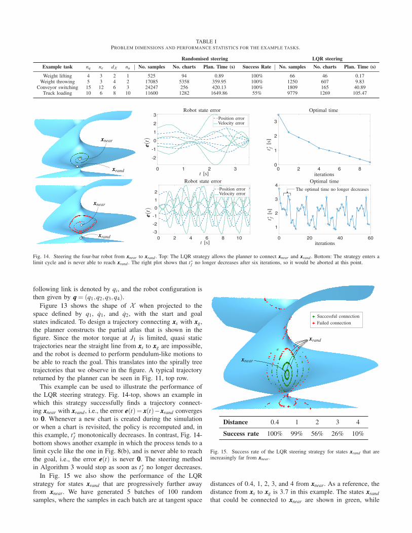
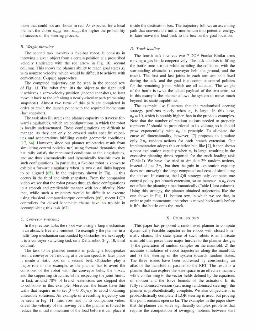
TABLE IPROBLEM DIMENSIONS AND PERFORMANCE STATISTICS FOR THE EXAMPLE TASKS.

Randomised steering LQR steering

Example task nq ne dX nu No. samples No. charts Plan. Time (s) Success Rate No. samples No. charts Plan. Time (s)

Weight lifting 4 3 2 1 525 94 0.89 100% 66 46 0.17Weight throwing 5 3 4 2 17085 5358 359.95 100% 1250 607 9.83

Conveyor switching 15 12 6 3 24247 256 420.13 100% 1809 165 40.89Truck loading 10 6 8 10 11600 1282 1649.86 55% 9779 1269 105.47

0 2 4 6 8 10

-3

-2

-1

0

1

2

0 20 40 60

1

2

3

4

0 1 2 3

-2

-1

0

1

2

3

0 2 4 6 80

1

2

3

xxxnear

xxxnear

xxxrand

xxxrand

ee e(t)

ee e(t)

Position error

Position error

Velocity error

Velocity error

t [s]

t [s]

t∗ f[s

]t∗ f

[s]

iterations

iterations

Optimal time

Optimal time

Robot state error

Robot state error

The optimal time no longer decreases

Fig. 14. Steering the four-bar robot from xxxnear to xxxrand . Top: The LQR strategy allows the planner to connect xxxnear and xxxrand . Bottom: The strategy enters alimit cycle and is never able to reach xxxrand . The right plot shows that t∗f no longer decreases after six iterations, so it would be aborted at this point.

following link is denoted by qi, and the robot configuration is

then given by qqq = (q1,q2,q3,q4).

Figure 13 shows the shape of X when projected to the

space defined by q1, q1, and q2, with the start and goal

states indicated. To design a trajectory connecting xxxs with xxxg,

the planner constructs the partial atlas that is shown in the

figure. Since the motor torque at J1 is limited, quasi static

trajectories near the straight line from xxxs to xxxg are impossible,

and the robot is deemed to perform pendulum-like motions to

be able to reach the goal. This translates into the spirally tree

trajectories that we observe in the figure. A typical trajectory

returned by the planner can be seen in Fig. 11, top row.

This example can be used to illustrate the performance of

the LQR steering strategy. Fig. 14-top, shows an example in

which this strategy successfully finds a trajectory connect-

ing xxxnear with xxxrand , i.e., the error eee(t) = xxx(t)−xxxrand converges

to 000. Whenever a new chart is created during the simulation

or when a chart is revisited, the policy is recomputed and, in

this example, t∗f monotonically decreases. In contrast, Fig. 14-

bottom shows another example in which the process tends to a

limit cycle like the one in Fig. 8(b), and is never able to reach

the goal, i.e., the error eee(t) is never 000. The steering method

in Algorithm 3 would stop as soon as t∗f no longer decreases.

In Fig. 15 we also show the performance of the LQR

strategy for states xxxrand that are progressively further away

from xxxnear. We have generated 5 batches of 100 random

samples, where the samples in each batch are at tangent space

xxxnear

xxxrand

Successful connection

Failed connection

Distance 0.4 1 2 3 4

Success rate 100% 99% 56% 26% 10%

Fig. 15. Success rate of the LQR steering strategy for states xxxrand that areincreasingly far from xxxnear .

distances of 0.4, 1, 2, 3, and 4 from xxxnear. As a reference, the

distance from xxxs to xxxg is 3.7 in this example. The states xxxrand

that could be connected to xxxnear are shown in green, while

those that could not are shown in red. As expected for a local

planner, the closer xxxrand from xxxnear, the higher the probability

of success of the steering process.

B. Weight throwing

The second task involves a five-bar robot. It consists in

throwing a given object from a certain position at a prescribed

velocity (indicated with the red arrow in Fig. 10, second

column). This shows the planner ability to reach goal states xxxg

with nonzero velocity, which would be difficult to achieve with

conventional C-space approaches.

The computed trajectory can be seen in the second row

of Fig. 11. The robot first lifts the object to the right until

it achieves a zero-velocity position (second snapshot), to later

move it back to the left along a nearly-circular path (remaining

snapshots). Almost two turns of this path are completed in

order to reach the launch point with the required momentum

(last snapshot).

The task also illustrates the planner capacity to traverse for-

ward singularities, which are configurations in which the robot

is locally underactuated. These configurations are difficult to

manage, as they can only be crossed under specific veloci-

ties and accelerations fulfilling certain geometric conditions

[17, 64]. However, since our planner trajectories result from

simulating control policies uuu(t) using forward dynamics, they

naturally satisfy the mentioned conditions at the singularities,

and are thus kinematically and dynamically feasible even in

such configurations. In particular, a five-bar robot is known to

exhibit a forward singularity when its two distal links happen

to be aligned [65]. In the trajectory shown in Fig. 11 this

occurs in the third and sixth snapshots. From the companion

video we see that the robot passes through these configurations

in a smooth and predictable manner with no difficulty. Note

that, while such a trajectory would be difficult to execute

using classical computed-torque controllers [66], recent LQR

controllers for closed kinematic chains have no trouble in

accomplishing this task [67].

C. Conveyor switching

In the previous tasks the robot was a single-loop mechanism

in an obstacle-free environment. To exemplify the planner in a

multi-loop mechanism surrounded by obstacles, we next apply

it to a conveyor switching task on a Delta robot (Fig. 10, third

column).

The task to be planned consists in picking a loudspeaker

from a conveyor belt moving at a certain speed, to later place

it inside a static box on a second belt. Obstacles play a

major role in this example, as the planner has to avoid the

collisions of the robot with the conveyor belts, the boxes,

and the supporting structure, while respecting the joint limits.

In fact, around 70% of branch extensions are stopped due

to collisions in this example. Moreover, the boxes have thin

walls that require us to set β = 0.05√

nX to avoid obtaining

unfeasible solutions. An example of a resulting trajectory can

be seen in Fig. 11, third row, and in its companion video.

Given the velocity of the moving belt, the planner is forced to

reduce the initial momentum of the load before it can place it

inside the destination box. The trajectory follows an ascending

path that converts the initial momentum into potential energy,

to later move the load back to the box on the goal location.

D. Truck loading

The fourth task involves two 7-DOF Franka Emika arms

moving a gas bottle cooperatively. The task consists in lifting

the bottle onto a truck while avoiding the collisions with the

surrounding obstacles (a conveyor belt, the ground, and the

truck). The first and last joints in each arm are held fixed

during the task, and the goal is to compute control policies

for the remaining joints, which are all actuated. The weight

of the bottle is twice the added payload of the two arms, so

in this example the planner allows the system to move much

beyond its static capabilities.

The example also illustrates that the randomised steering

strategy performs poorly when nu is large. In this case,

nu = 10, which is notably higher than in the previous examples.

Note that the number of random actions needed to properly

represent U should be proportional to its volume, so it should

grow exponentially with nu in principle. To alleviate the

curse of dimensionality, however, [7] proposes to simulate

only 2 nu random actions for each branch extension. Our

implementation adopts this criterion but, like [7], it then shows

a poor exploration capacity when nu is large, resulting in the

excessive planning times reported for the truck loading task

(Table I). We have also tried to simulate 2nu random actions,

instead of just 2 nu, but then the gain in exploration capacity

does not outweigh the large computational cost of simulating

the actions. In contrast, the LQR strategy only computes one

control policy per branch extension, so an increase in nu does

not affect the planning time dramatically (Table I, last column).

Using this strategy, the planner obtained trajectories like the

one shown in Fig. 11, bottom row, in which we see that, in

order to gain momentum, the robot is moved backwards before

it lifts the bottle onto the truck.

X. CONCLUSIONS

This paper has proposed a randomised planner to compute

dynamically-feasible trajectories for robots with closed kine-

matic chains. The state space of such robots is an intricate

manifold that poses three major hurdles to the planner design:

1) the generation of random samples on the manifold; 2) the

accurate simulation of robot trajectories along the manifold;

and 3) the steering of the system towards random states.

The three issues have been addressed by constructing an

atlas of the manifold in parallel to the RRT. The result is a

planner that can explore the state space in an effective manner,

while conforming to the vector fields defined by the equations

of motion and the force bounds of the actuators. In its

fully randomised version (i.e., using randomised steering), the

planner is probabilistically complete. We also conjecture it is

probabilistically complete if LQR steering is used, but proving

this point remains open so far. The examples in the paper show

that the planner can solve significantly complex problems that

require the computation of swinging motions between start

and goal states, under restrictive torque limitations imposed

on the motors.

Several points should be considered in further improvements

of this work. Note that, as usual in a randomised planner,

our control policies are piecewise continuous, so the planned

trajectories are smooth in position, but not in velocity or

acceleration. Therefore, to reduce control or vibration issues

in practice, a post-processing should be applied to obtain

twice differentiable trajectories. The trajectories should also be

optimised in some sense, minimising the time or control effort

required for its execution. Trajectory optimization tools like

those in [38], [41], or [42] might be very helpful to both ends.

Another sensitive point is the metric employed to measure

the distance between states. This is a general concern in any

motion planner, but it is more difficult to address in our context

as such metric should not only consider the vector flows de-

fined by the equations of motion, but also the curvature of the

state space manifold defined by the loop-closure constraints.

Using a metric derived from geometric insights provided

by such constraints might result in substantial performance

improvements. Another point deserving attention would be

the monitoring of constraint forces during the extension of

the RRT. While such forces result in no motion, they do

stress the robot parts unnecessarily and should be kept under

admissible bounds. Note that these forces can be computed

as the simulations proceed, since they can be inferred, e.g.,

from the values of the Lagrange multipliers involved in the

equations of motion [68]. The ability to impose bounds on

constraint forces would also allow computing trajectories in

closed kinematic chains induced by unilateral contacts, like

those that arise when a hand moves an object in contact with a

surface. Such contacts could be maintained along a trajectory

by setting pertinent signed bounds on the constraint forces

arising.

REFERENCES

[1] B. Donald, P. Xavier, J. Canny, and J. Reif, “Kinodynamic motionplanning,” Journal of the ACM, vol. 40, no. 5, pp. 1048–1066, 1993.

[2] S.-H. Lee, J. Kim, F. C. Park, M. Kim, and J. E. Bobrow, “Newton-typealgorithms for dynamics-based robot movement optimization,” IEEE

Transactions on robotics, vol. 21, no. 4, pp. 657–667, 2005.

[3] I. Bonev, “Delta parallel robot - the story of success,” Newsletter,

available at http://www.parallemic.org, 2001.

[4] S. Feng, E. Whitman, X. Xinjilefu, and C. G. Atkeson, “Optimizationbased full body control for the atlas robot,” in IEEE-RAS International

Conference on Humanoid Robots, 2014, pp. 120–127.

[5] M. A. Diftler, J. S. Mehling, M. E. Abdallah, N. A. Radford, L. B.Bridgwater, A. M. Sanders, R. S. Askew, D. M. Linn, J. D. Yamokoski,F. A. Permenter, B. K. Hargrave, R. Platt, R. T. Savely, and R. O.Ambrose, “Robonaut 2 - the first humanoid robot in space,” in 2011

IEEE International Conference on Robotics and Automation, 2011, pp.2178–2183.

[6] R. P. Hoyt, “Spiderfab: An architecture for self-fabricating space sys-tems,” in AIAA Space 2013 Conference and Exposition, 2013, p. 5509.

[7] S. M. LaValle and J. J. Kuffner, “Randomized kinodynamic planning,”International Journal of Robotics Research, vol. 20, no. 5, pp. 378–400,2001.

[8] Y. Li, Z. Littlefield, and K. E. Bekris, “Asymptotically optimal sampling-based kinodynamic planning,” The International Journal of Robotics

Research, vol. 35, no. 5, pp. 528–564, 2016.

[9] K. Hauser and Y. Zhou, “Asymptotically optimal planning by feasiblekinodynamic planning in a state–cost space,” IEEE Transactions on

Robotics, vol. 32, no. 6, pp. 1431–1443, 2016.

[10] D. Berenson, S. Srinivasa, and J. J. Kuffner, “Task space regions: Aframework for pose-constrained manipulation planning,” International

Journal of Robotics Research, vol. 30, no. 12, pp. 1435–1460, 2011.

[11] J. M. Porta, L. Jaillet, and O. Bohigas, “Randomized path planning onmanifolds based on higher-dimensional continuation,” The International

Journal of Robotics Research, vol. 31, no. 2, pp. 201–215, 2012.

[12] L. Jaillet and J. M. Porta, “Path planning under kinematic constraints byrapidly exploring manifolds,” IEEE Transactions on Robotics, vol. 29,no. 1, pp. 105–117, 2013.

[13] K. Hauser, “Fast interpolation and time-optimization with contact,” The

International Journal of Robotics Research, vol. 33, no. 9, pp. 1231–1250, 2014.

[14] Q.-C. Pham and O. Stasse, “Time-optimal path parameterizationfor redundantly actuated robots: A numerical integration approach,”IEEE/ASME Transactions on Mechatronics, vol. 20, no. 6, pp. 3257–3263, 2015.

[15] Z. Kingston, M. Moll, and L. E. Kavraki, “Decoupling constraintsfrom sampling-based planners,” in International Symposium of Robotics

Research, 2017.

[16] ——, “Sampling-based methods for motion planning with constraints,”Annual Review of Control, Robotics, and Autonomous Systems, vol. 1,pp. 159–185, 2018.

[17] O. Bohigas, M. Manubens, and L. Ros, Singularities of robot mech-

anisms: Numerical computation and avoidance path planning, ser.Mechanisms and Machine Science. Springer, 2017, vol. 41.

[18] R. Bordalba, L. Ros, and J. M. Porta, “Randomized kinodynamicplanning for constrained systems,” in IEEE International Conference

on Robotics and Automation, 2018, pp. 7079–7086.

[19] J. H. Yakey, S. M. LaValle, and L. E. Kavraki, “Randomized pathplanning for linkages with closed kinematic chains,” IEEE Transactions

on Robotics and Automation, vol. 17, no. 6, pp. 951–959, 2001.

[20] L. Han and N. M. Amato, “A kinematics-based probabilistic roadmapmethod for closed chain systems,” in Algorithmic and Computational

Robotics - New Directions, 2000, pp. 233–246.

[21] J. Cortés, T. Siméon, and J.-P. Laumond, “A random loop generator forplanning the motions of closed kinematic chains using PRM methods,”in IEEE International Conference on Robotics and Automation, 2002,pp. 2141–2146.

[22] M. Stilman, “Task constrained motion planning in robot joint space,” inIEEE/RSJ International Conference on Intelligent Robots and Systems,2007, pp. 3074–3081.

[23] B. Kim, T. T. Um, C. Suh, and F. C. Park, “Tangent bundle RRT:A randomized algorithm for constrained motion planning,” Robotica,vol. 34, no. 1, pp. 202–225, 2016.

[24] S. M. LaValle, Planning algorithms. New York: Cambridge UniversityPress, 2006.

[25] H. Choset, K. M. Lynch, S. Hutchinson, G. A. Kantor, W. Burgard, L. E.Kavraki, and S. Thrun, Principles of robot motion: theory, algorithms,

and implementations, ser. Intelligent Robotics and Autonomous Agents.MIT Press, 2005.

[26] J. E. Bobrow, S. Dubowsky, and J. Gibson, “Time-optimal control ofrobotic manipulators along specified paths,” The International Journal

of Robotics Research, vol. 4, no. 3, pp. 3–17, 1985.

[27] K. Shin and N. McKay, “Minimum-time control of robotic manipulatorswith geometric path constraints,” IEEE Transactions on Automatic

Control, vol. 30, no. 6, pp. 531–541, 1985.

[28] F. Pfeiffer and R. Johanni, “A concept for manipulator trajectoryplanning,” IEEE Journal on Robotics and Automation, vol. 3, no. 2,pp. 115–123, 1987.

[29] J.-J. Slotine and H. S. Yang, “Improving the efficiency of time-optimalpath-following algorithms,” IEEE Transactions on Robotics and Automa-

tion, vol. 5, no. 1, pp. 118–124, 1989.

[30] Z. Shiller and H.-H. Lu, “Computation of path constrained time optimalmotions with dynamic singularities,” Journal of Dynamic Systems,

Measurement, and Control, vol. 114, no. 1, pp. 34–40, 1992.

[31] Q.-C. Pham, “A general, fast, and robust implementation of thetime-optimal path parameterization algorithm,” IEEE Transactions on

Robotics, vol. 30, no. 6, pp. 1533–1540, 2014.

[32] Q.-C. Pham, S. Caron, P. Lertkultanon, and Y. Nakamura, “Admissi-ble velocity propagation: Beyond quasi-static path planning for high-dimensional robots,” The International Journal of Robotics Research,vol. 36, no. 1, pp. 44–67, 2017.

[33] J. E. Bobrow, “Optimal robot path planning using the minimum-timecriterion,” IEEE Journal on Robotics and Automation, vol. 4, no. 4, pp.443–450, 1988.

[34] Z. Shiller and S. Dubowsky, “Robot path planning with obstacles,actuator, gripper, and payload constraints,” The International Journal

of Robotics Research, vol. 8, no. 6, pp. 3–18, 1989.

[35] Z. Shiller and S. Dubowsky, “On computing the global time-optimalmotions of robotic manipulators in the presence of obstacles,” IEEE

Transactions on Robotics and Automation, vol. 7, no. 6, pp. 785–797,Dec 1991.

[36] Q.-C. Pham, S. Caron, and Y. Nakamura, “Kinodynamic planning in theconfiguration space via admissible velocity propagation,” in Robotics:

Science and Systems, 2013.

[37] M. Kalakrishnan, S. Chitta, E. Theodorou, P. Pastor, and S. Schaal,“STOMP: Stochastic trajectory optimization for motion planning,” inIEEE International Conference on Robotics and Automation, 2011, pp.4569–4574.

[38] M. Posa, S. Kuindersma, and R. Tedrake, “Optimization and stabilizationof trajectories for constrained dynamical systems,” in IEEE International

Conference on Robotics and Automation, 2016, pp. 1366–1373.

[39] J. Schulman, D. Y, J. Ho, A. Lee, I. Awwal, H. Bradlow, J. Pan, S. Patil,K. Goldberg, and P. Abbeel, “Motion planning with sequential convexoptimization and convex collision checking,” The International Journal

of Robotics Research, vol. 33, no. 9, pp. 1251–1270, 2014.

[40] M. Zucker, N. Ratliff, A. D. Dragan, M. Pivtoraiko, M. Klingensmith,C. M. Dellin, J. A. Bagnell, and S. S. Srinivasa, “CHOMP: Covari-ant Hamiltonian optimization for motion planning,” The International

Journal of Robotics Research, vol. 32, no. 9-10, pp. 1164–1193, 2013.

[41] J. T. Betts, Practical methods for optimal control and estimation using

nonlinear programming. SIAM Publications, 2010.

[42] ——, “Survey of numerical methods for trajectory optimization,” Jour-

nal of Guidance, Control, and Dynamics, vol. 21, no. 2, pp. 193–207,1998.

[43] T. Kunz and M. Stilman, “Probabilistically complete kinodynamicplanning for robot manipulators with acceleration limits,” in IEEE/RSJ

International Conference on Intelligent Robots and Systems, 2014, pp.3713–3719.

[44] A. Perez, R. Platt, G. Konidaris, L. Kaelbling, and T. Lozano-Perez,“LQR-RRT*: Optimal sampling-based motion planning with automat-ically derived extension heuristics,” in IEEE International Conference

on Robotics and Automation, 2012, pp. 2537–2542.

[45] R. Tedrake, “LQR-Trees: Feedback motion planning on sparse random-ized trees,” in Robotics: Science and Systems, 2009.

[46] G. Goretkin, A. Perez, R. Platt, and G. Konidaris, “Optimal sampling-based planning for linear-quadratic kinodynamic systems,” in IEEE

International Conference on Robotics and Automation, 2013, pp. 2429–2436.

[47] D. J. Webb and J. van den Berg, “Kinodynamic RRT*: Asymptoticallyoptimal motion planning for robots with linear dynamics,” in IEEE

International Conference on Robotics and Automation, 2013, pp. 5054–5061.

[48] R. Bordalba, L. Ros, and J. M. Porta, “A randomized kinodynamic plan-ner for closed-chain robotic systems,” Institut de Robòtica i Infomàtica.CSIC-UPC. Technical Report, 2019, https://bit.ly/2vk4MSO.

[49] F. A. Potra and J. Yen, “Implicit numerical integration for Euler-Lagrange equations via tangent space parametrization,” Journal of

Structural Mechanics, vol. 19, no. 1, pp. 77–98, 1991.

[50] L. R. Petzold, “Numerical solution of differential-algebraic equationsin mechanical systems simulation,” Physica D: Nonlinear Phenomena,vol. 60, no. 1–4, pp. 269–279, 1992.

[51] R. Featherstone and D. E. Orin, “Dynamics,” in Springer Handbook of

Robotics. Springer, 2016, pp. 37–66.[52] W. Blajer, “Methods for constraint violation suppression in the numerical

simulation of constrained multibody systems - A comparative study,”Computer Methods in Applied Mechanics and Engineering, vol. 200,no. 13-16, pp. 1568–1576, 2011.

[53] M. E. Henderson, “Multiple parameter continuation: computing im-plicitly defined k-manifolds,” International Journal of Bifurcation and

Chaos, vol. 12, no. 3, pp. 451–476, 2002.[54] E. Hairer, “Geometric integration of ordinary differential equations on

manifolds,” BIT Numerical Mathematics, vol. 41, no. 5, pp. 996–1007,2001.

[55] E. Hairer, C. Lubich, and G. Wanner, “Geometric numerical integra-tion: structure-preserving algorithms for ordinary differential equations,”2006.

[56] F. L. Lewis, D. Vrabie, and V. L. Syrmos, Optimal control. John Wiley& Sons, 2012.

[57] D. P. Bertsekas, Dynamic programming and optimal control. AthenaScientific, 2005.

[58] J. Kuffner and S. M. LaValle, “RRT-connect: An efficient approachto single-query path planning,” in IEEE International Conference on

Robotics and Automation, vol. 2, 2000, pp. 995–1001.[59] J. M. Porta and L. Jaillet, “Sampling strategies for path planning under

kinematic constraints,” CoRR, vol. abs/1407.2544, 2014.[60] A. E. Bryson and Y.-C. Ho, Applied Optimal Control: Optimization,

Estimation and Control. Taylor Francis, 1975.[61] M. Kleinbort, K. Solovey, Z. Littlefield, K. E. Bekris, and D. Halperin,

“Probabilistic completeness of RRT for geometric and kinodynamicplanning with forward propagation,” IEEE Robotics and Automation

Letters, vol. 4, no. 3, pp. 277–283, 2019.[62] L. Jaillet and J. M. Porta, “Efficient asymptotically-optimal path plan-

ning on manifolds,” Robotics and Autonomous Systems, vol. 61, no. 8,pp. 797–807, 2013.

[63] J. M. Porta, L. Ros, O. Bohigas, M. Manubens, C. Rosales, and L. Jaillet,“The Cuik Suite: Analyzing the motion of closed-chain multibodysystems,” IEEE Robotics and Automation Magazine, vol. 21, no. 3, pp.105–114, 2014.

[64] S. Briot and V. Arakelian, “Optimal force generation in parallel ma-nipulators for passing through the singular positions,” The International

Journal of Robotics Research, vol. 27, no. 8, pp. 967–983, 2008.[65] F. Bourbonnais, P. Bigras, and I. A. Bonev, “Minimum-time trajec-

tory planning and control of a pick-and-place five-bar parallel robot,”IEEE/ASME Transactions on Mechatronics, vol. 20, no. 2, pp. 740–749,2015.

[66] F. Aghili, “A unified approach for inverse and direct dynamics ofconstrained multibody systems based on linear projection operator:applications to control and simulation,” IEEE Transactions on Robotics,vol. 21, no. 5, pp. 834–849, 2005.

[67] R. Bordalba, J. M. Porta, and L. Ros, “A singularity-robust LQRcontroller for parallel robots,” in IEEE/RSJ International Conference

on Intelligent Robots and Systems, 2018, pp. 270–276.[68] R. Featherstone, Robot dynamics algorithms. Kluwer, Norwell, MA,

1987.