A rational cubic spline for the visualization of monotonic data: an alternate approach

Computers & Graphics 27 (2003) 107–121

Technical section

A rational cubic spline for the visualization of monotonic data:an alternate approach

M. Sarfraz*

Department of Information and Computer Science, King Fahd University of Petroleum and Minerals, KFUPM # 1510,

Dhahran 31261, Saudi Arabia

Accepted 18 October 2002

Abstract

A smooth curve interpolation scheme for monotonic data was developed by Sarfraz (Comput. Graph. 24(4) (2000)

509). This scheme is reviewed and a new alternate approach, which was indicated in Sarfraz (Comput. Graph. 26(1)

(2002) 193), has been introduced with all details and solid proofs here. In theory, the new scheme uses the same

piecewise rational cubic functions as in Sarfraz (2000), but it utilizes a rational quadratic in practice. The two families of

parameters, in the description of the rational interpolant, have been constrained to preserve the monotone shape of the

data. The new rational spline scheme, like the old one in Sarfraz, 2000, has a unique representation. The degree of

smoothness attained is C2 and the method of computation is robust.

Both, old as well as new shape preserving methods, seem to be equally competent. This is shown by a comparative

analysis. There is a trade off between the two methods as far as computational aspects are concerned. However, the new

method is superior to the old method as far as accuracy is concerned. This fact has been proved by making an error

analysis over the actual and computed curves.

r 2002 Elsevier Science Ltd. All rights reserved.

Keywords: Data visualization; Rational spline; Interpolation; Shape preserving; Monotone

1. Introduction

Smooth curve representation, to visualize the scientific

data, is of great significance in the area of Computer

Graphics and in particular Data Visualization. Particu-

larly, when the data is obtained from some complex

function or from some scientific phenomena, it becomes

crucial to incorporate the inherited features of the data.

Moreover, smoothness is also one of the very important

requirements for pleasing visual display. Ordinary spline

schemes, although smoother, are not helpful for the

interpolation of the shaped data. Severely misleading

results, violating the inherent features of the data, are

seen when undesired oscillations occur. For example, for

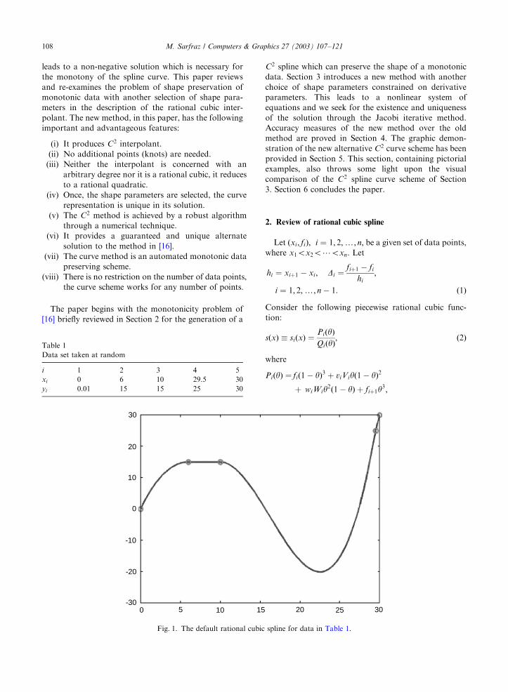
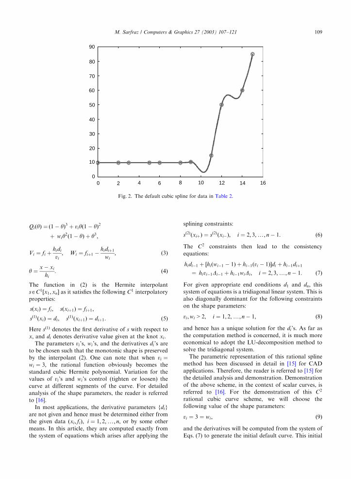
the data sets in Table 1 (data taken randomly) and Table

2 (Akima’s data [3]), their corresponding curves in

Figs. 1 and 2, respectively, are not as may be desired by

the user for a monotonically increasing data. The user

would visualize them as they appear in Figs. 5 and 6,

respectively. Thus, unwanted oscillations which com-

pletely distort the data features, need to be controlled.

Various authors have discussed this issue. For brevity,

the reader is referred to [1–19].

This paper reviews the method of shape preservation

of monotonic data in [16] and introduces a new alternate

approach, indicated in [19]. The motivation to this work

is due to some observations in the past work [16] of the

author. One observation was that the shape parameters,

in the description of the rational cubic interpolant, were

restricted to a particular choice. But, the author

observed equally good results for another choice too.

Another observation made was that there is no

guarantee that the system of linear equations, in [16],*Tel.: +966-3-860-2763; fax: +966-3-860-1562.

E-mail address: [email protected] (M. Sarfraz).

0097-8493/03/$ - see front matter r 2002 Elsevier Science Ltd. All rights reserved.

PII: S 0 0 9 7 - 8 4 9 3 ( 0 2 ) 0 0 2 4 9 - 2

leads to a non-negative solution which is necessary for

the monotony of the spline curve. This paper reviews

and re-examines the problem of shape preservation of

monotonic data with another selection of shape para-

meters in the description of the rational cubic inter-

polant. The new method, in this paper, has the following

important and advantageous features:

(i) It produces C2 interpolant.

(ii) No additional points (knots) are needed.

(iii) Neither the interpolant is concerned with an

arbitrary degree nor it is a rational cubic, it reduces

to a rational quadratic.

(iv) Once, the shape parameters are selected, the curve

representation is unique in its solution.

(v) The C2 method is achieved by a robust algorithm

through a numerical technique.

(vi) It provides a guaranteed and unique alternate

solution to the method in [16].

(vii) The curve method is an automated monotonic data

preserving scheme.

(viii) There is no restriction on the number of data points,

the curve scheme works for any number of points.

The paper begins with the monotonicity problem of

[16] briefly reviewed in Section 2 for the generation of a

C2 spline which can preserve the shape of a monotonic

data. Section 3 introduces a new method with another

choice of shape parameters constrained on derivative

parameters. This leads to a nonlinear system of

equations and we seek for the existence and uniqueness

of the solution through the Jacobi iterative method.

Accuracy measures of the new method over the old

method are proved in Section 4. The graphic demon-

stration of the new alternative C2 curve scheme has been

provided in Section 5. This section, containing pictorial

examples, also throws some light upon the visual

comparison of the C2 spline curve scheme of Section

3. Section 6 concludes the paper.

2. Review of rational cubic spline

Let ðxi; fiÞ; i ¼ 1; 2;y; n; be a given set of data points,where x1ox2o?oxn: Let

hi ¼ xiþ1 � xi; Di ¼fiþ1 � fi

hi

;

i ¼ 1; 2;y; n � 1: ð1Þ

Consider the following piecewise rational cubic func-

tion:

sðxÞ � siðxÞ ¼PiðyÞQiðyÞ

; ð2Þ

where

PiðyÞ ¼ fið1� yÞ3 þ viViyð1� yÞ2

þ wiWiy2ð1� yÞ þ fiþ1y

3;

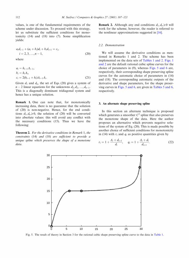
Table 1

Data set taken at random

i 1 2 3 4 5

xi 0 6 10 29.5 30

yi 0.01 15 15 25 30

30

20

10

0

-10

-20

-300 5 10 15 20 25 30

Fig. 1. The default rational cubic spline for data in Table 1.

M. Sarfraz / Computers & Graphics 27 (2003) 107–121108

QiðyÞ ¼ ð1� yÞ3 þ viyð1� yÞ2

þ wiy2ð1� yÞ þ y3;

Vi ¼ fi þhidi

vi

; Wi ¼ fiþ1 �hidiþ1

wi

; ð3Þ

y ¼x � xi

hi

: ð4Þ

The function in (2) is the Hermite interpolant

sAC1½x1; xn� as it satisfies the following C1 interpolatory

properties:

sðxiÞ ¼ fi; sðxiþ1Þ ¼ fiþ1;

sð1ÞðxiÞ ¼ di; sð1Þðxiþ1Þ ¼ diþ1: ð5Þ

Here sð1Þ denotes the first derivative of s with respect to

x; and di denotes derivative value given at the knot xi:The parameters vi’s, wi’s, and the derivatives di’s are

to be chosen such that the monotonic shape is preserved

by the interpolant (2). One can note that when vi ¼wi ¼ 3; the rational function obviously becomes the

standard cubic Hermite polynomial. Variation for the

values of vi’s and wi’s control (tighten or loosen) the

curve at different segments of the curve. For detailed

analysis of the shape parameters, the reader is referred

to [16].

In most applications, the derivative parameters fdigare not given and hence must be determined either from

the given data ðxi; fiÞ; i ¼ 1; 2;y; n; or by some other

means. In this article, they are computed exactly from

the system of equations which arises after applying the

splining constraints:

sð2ÞðxiþÞ ¼ sð2Þðxi�Þ; i ¼ 2; 3;y; n � 1: ð6Þ

The C2 constraints then lead to the consistency

equations:

hidi�1 þ ½hiðwi�1 � 1Þ þ hi�1ðvi � 1Þ�di þ hi�1diþ1

¼ hivi�1Di�1 þ hi�1wiDi; i ¼ 2; 3;y; n � 1: ð7Þ

For given appropriate end conditions d1 and dn; thissystem of equations is a tridiagonal linear system. This is

also diagonally dominant for the following constraints

on the shape parameters:

vi ;wi > 2; i ¼ 1; 2;y; n � 1; ð8Þ

and hence has a unique solution for the di’s. As far as

the computation method is concerned, it is much more

economical to adopt the LU-decomposition method to

solve the tridiagonal system.

The parametric representation of this rational spline

method has been discussed in detail in [15] for CAD

applications. Therefore, the reader is referred to [15] for

the detailed analysis and demonstration. Demonstration

of the above scheme, in the context of scalar curves, is

referred to [16]. For the demonstration of this C2

rational cubic curve scheme, we will choose the

following value of the shape parameters:

vi ¼ 3 ¼ wi; ð9Þ

and the derivatives will be computed from the system of

Eqs. (7) to generate the initial default curve. This initial

90

80

70

60

50

40

30

20

10

00 2 4 6 8 10 12 14 16

Fig. 2. The default cubic spline for data in Table 2.

M. Sarfraz / Computers & Graphics 27 (2003) 107–121 109

default curve is actually the same as a cubic spline curve.

Further modifications can be made by changing these

parameters.

The rational spline method, described above, has

deficiencies as far as the shape preserving issue is

concerned. For example, in Fig. 1, it does not preserve

the shape of the monotonic data of Table 1. Very clearly,

this curve is not preserving the shape of the data. It is

required to assign appropriate values to the shape

parameters so that they generate a data preserved shape.

Similarly an unwanted behaviour can be observed in

Fig. 2 for the data set in Table 2. Thus, it looks as if

ordinary spline schemes do not provide the desired

shape features and hence some further treatment is

required to achieve a shape preserving spline for

monotone data.

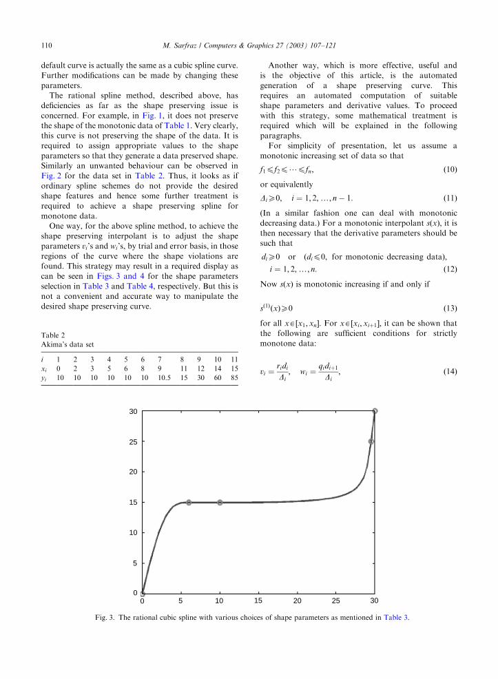
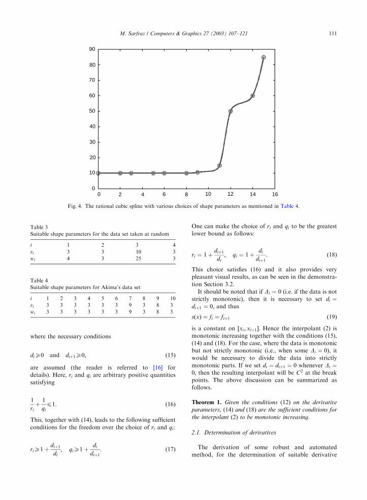
One way, for the above spline method, to achieve the

shape preserving interpolant is to adjust the shape

parameters vi’s and wi’s, by trial and error basis, in those

regions of the curve where the shape violations are

found. This strategy may result in a required display as

can be seen in Figs. 3 and 4 for the shape parameters

selection in Table 3 and Table 4, respectively. But this is

not a convenient and accurate way to manipulate the

desired shape preserving curve.

Another way, which is more effective, useful and

is the objective of this article, is the automated

generation of a shape preserving curve. This

requires an automated computation of suitable

shape parameters and derivative values. To proceed

with this strategy, some mathematical treatment is

required which will be explained in the following

paragraphs.

For simplicity of presentation, let us assume a

monotonic increasing set of data so that

f1pf2p?pfn; ð10Þ

or equivalently

DiX0; i ¼ 1; 2;y; n � 1: ð11Þ

(In a similar fashion one can deal with monotonic

decreasing data.) For a monotonic interpolant sðxÞ; it isthen necessary that the derivative parameters should be

such that

diX0 or ðdip0; for monotonic decreasing dataÞ;

i ¼ 1; 2;y; n: ð12Þ

Now sðxÞ is monotonic increasing if and only if

sð1ÞðxÞX0 ð13Þ

for all xA½x1; xn�: For xA½xi;xiþ1�; it can be shown that

the following are sufficient conditions for strictly

monotone data:

vi ¼ridi

Di

; wi ¼qidiþ1

Di

; ð14Þ

30

25

20

15

10

5

00 5 10 15 20 25 30

Fig. 3. The rational cubic spline with various choices of shape parameters as mentioned in Table 3.

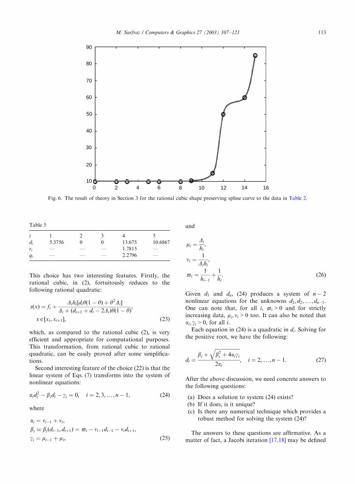
Table 2

Akima’s data set

i 1 2 3 4 5 6 7 8 9 10 11

xi 0 2 3 5 6 8 9 11 12 14 15

yi 10 10 10 10 10 10 10.5 15 30 60 85


where the necessary conditions

diX0 and diþ1X0; ð15Þ

are assumed (the reader is referred to [16] for

details). Here, ri and qi are arbitrary positive quantities

satisfying

1

ri

þ1

qi

p1: ð16Þ

This, together with (14), leads to the following sufficient

conditions for the freedom over the choice of ri and qi:

riX1þdiþ1

di

; qiX1þdi

diþ1: ð17Þ

One can make the choice of ri and qi to be the greatest

lower bound as follows:

ri ¼ 1þdiþ1

di

; qi ¼ 1þdi

diþ1: ð18Þ

This choice satisfies (16) and it also provides very

pleasant visual results, as can be seen in the demonstra-

tion Section 3.2.

It should be noted that if Di ¼ 0 (i.e. if the data is not

strictly monotonic), then it is necessary to set di ¼diþ1 ¼ 0; and thus

sðxÞ ¼ fi ¼ fiþ1 ð19Þ

is a constant on ½xi; xiþ1�: Hence the interpolant (2) is

monotonic increasing together with the conditions (15),

(14) and (18). For the case, where the data is monotonic

but not strictly monotonic (i.e., when some Di ¼ 0), it

would be necessary to divide the data into strictly

monotonic parts. If we set di ¼ diþ1 ¼ 0 whenever Di ¼0; then the resulting interpolant will be C2 at the break

points. The above discussion can be summarized as

follows.

Theorem 1. Given the conditions (12) on the derivative

parameters, (14) and (18) are the sufficient conditions for

the interpolant (2) to be monotonic increasing.

2.1. Determination of derivatives

The derivation of some robust and automated

method, for the determination of suitable derivative

90

80

70

60

50

40

30

20

10

00 2 4 6 8 10 12 14 16

Fig. 4. The rational cubic spline with various choices of shape parameters as mentioned in Table 4.

Table 3

Suitable shape parameters for the data set taken at random

i 1 2 3 4

vi 3 3 10 3

wi 4 3 25 3

Table 4

Suitable shape parameters for Akima’s data set

i 1 2 3 4 5 6 7 8 9 10

vi 3 3 3 3 3 3 9 3 8 3

wi 3 3 3 3 3 3 9 3 8 3


values, is one of the fundamental requirements of the

scheme under discussion. To proceed with this strategy,

let us substitute the sufficient conditions for mono-

tonicity (14) and (18) into (7). Some simplification

yields:

aidi�1 þ ðai þ biÞdi þ bidiþ1 ¼ ci;

i ¼ 2; 3;y; n � 1; ð20Þ

where

ai ¼ hi�1Di�1;

bi ¼ hiDi;

ci ¼ 2ðhi�1 þ hiÞDi�1Di: ð21Þ

Given d1 and dn; the set of Eqs. (20) gives a system of

n � 2 linear equations for the unknowns d2; d2;y; dn�1:This is a diagonally dominant tridiagonal system and

hence has a unique solution.

Remark 1. One can note that, for monotonically

increasing data, there is no guarantee that the solution

of (20) is non-negative. Hence, for the end condi-

tions d1; dnX0; the solution of (20) will be converted

into absolute values: this will avoid any conflict with

the necessary conditions (15). Thus we have the

following:

Theorem 2. For the derivative conditions in Remark 1, the

constraints (14) and (18) are sufficient to provide a

unique spline which preserves the shape of a monotone

data.

Remark 2. Although any end conditions d1; dnX0 will

work for the scheme, however, the reader is referred to

the nonlinear approximations suggested in [16].

2.2. Demonstration

We will assume the derivative conditions as men-

tioned in Remarks 1 and 2. The scheme has been

implemented on the data sets of Tables 1 and 2. Figs. 1

and 2 are the default rational cubic spline curves for the

choice of parameters in (9), whereas Figs. 5 and 6 are,

respectively, their corresponding shape preserving spline

curves for the automatic choice of parameters in (14)

and (18). The corresponding automatic outputs of the

derivative and shape parameters, for the shape preser-

ving curves in Figs. 5 and 6, are given in Tables 5 and 6,

respectively.

3. An alternate shape preserving spline

In this section an alternate technique is proposed

which generates a smoother C2 spline that also preserves

the monotone shape of the data. Here the author

proposes an alternative which prevents negative solu-

tions of the system of Eq. (20). This is made possible by

another choice of sufficient conditions for monotonicity

in (14) with ri and qi as positive quantities given by

ri ¼ 1þDi þ diþ1

di

; qi ¼ 1þDi þ di

diþ1: ð22Þ

30

25

20

15

10

5

00 5 10 15 20 25 30

Fig. 5. The result of theory in Section 3 for the rational cubic shape preserving spline curve to the data in Table 1.


This choice has two interesting features. Firstly, the

rational cubic, in (2), fortuitously reduces to the

following rational quadratic:

sðxÞ ¼ fi þDihi½diyð1� yÞ þ y2Di�

Di þ ðdiþ1 þ di � 2DiÞyð1� yÞ;

xA½xi; xiþ1�; ð23Þ

which, as compared to the rational cubic (2), is very

efficient and appropriate for computational purposes.

This transformation, from rational cubic to rational

quadratic, can be easily proved after some simplifica-

tions.

Second interesting feature of the choice (22) is that the

linear system of Eqs. (7) transforms into the system of

nonlinear equations:

aid2i � bidi � gi ¼ 0; i ¼ 2; 3;y; n � 1; ð24Þ

where

ai ¼ ni�1 þ ni;

bi � biðdi�1; diþ1Þ ¼ $ i � ni�1di�1 � nidiþ1;

gi ¼ mi�1 þ mi; ð25Þ

and

mi ¼Di

hi

;

ni ¼1

Dihi

;

$ i ¼1

hi�1þ

1

hi

: ð26Þ

Given d1 and dn; (24) produces a system of n � 2

nonlinear equations for the unknowns d2; d2;y; dn�1:One can note that, for all i; $ i > 0 and for strictly

increasing data, mi ; ni > 0 too. It can also be noted that

ai; gi > 0; for all i:Each equation in (24) is a quadratic in di: Solving for

the positive root, we have the following:

di ¼bi þ

ffiffiffiffiffiffiffiffiffiffiffiffiffiffiffiffiffiffiffiffib2i þ 4aigi

q2ai

; i ¼ 2;y; n � 1: ð27Þ

After the above discussion, we need concrete answers to

the following questions:

(a) Does a solution to system (24) exists?

(b) If it does, is it unique?

(c) Is there any numerical technique which provides a

robust method for solving the system (24)?

The answers to these questions are affirmative. As a

matter of fact, a Jacobi iteration [17,18] may be defined

90

80

70

60

50

40

30

20

100 2 4 6 8 10 12 14 16


Table 5

i 1 2 3 4 5

di 5.3756 0 0 13.675 10.6867

ri — — — 1.7815 —

qi — — — 2.2796 —


as follows:

dðkþ1Þi ¼

bðkÞi þffiffiffiffiffiffiffiffiffiffiffiffiffiffiffiffiffiffiffiffiffiffiffiffiffiffiffiffiðbðkÞi Þ2 þ 4aigi

q2ai

;

i ¼ 2;y; n � 1 ð28Þ

where

bðkÞi ¼ biðdðkÞi�1; d

ðkÞiþ1Þ; i ¼ 2;y; n � 1; ð29Þ

and

dðkþ1Þ1 ¼ d

ðkÞ1 ¼ d1 and dðkþ1Þ

n ¼ dðkÞn ¼ dn ð30Þ

are the given end conditions. This leads to the following

theorem.

Theorem 3. For strictly increasing data and given

end conditions d1X0 and dnX0; there exists a unique

solution d2;y; dn�1 satisfying the nonlinear consistency

equation (24) and the monotonicity conditions diX0;i ¼ 2; 3;y; n � 1:

Proof. Let us initially define a set of functions Ji; i ¼1; 2;y; n on the domain Rn by

J1ðcÞ ¼ d1;

JiðcÞ ¼biðci�1;ciþ1Þ þ

ffiffiffiffiffiffiffiffiffiffiffiffiffiffiffiffiffiffiffiffiffiffiffiffiffiffiffiffiffiffiffiffiffiffiffiffiffiffiffiffiffiffiffib2i ðci�1;ciþ1Þ þ 4aigi

q2ai

;

i ¼ 2;y; n � 1; ð31Þ

JnðcÞ ¼ dn;

where w ¼ ðci ;y;cnÞARn: Let J ¼ ðJ1;y; JnÞ and d ¼ðd1;y; dnÞ: Then the Jacobi iteration (28) takes the form

dðkþ1Þ ¼ Jðd ðkÞÞ:

It can be noted that the numerator in (31) is a

monotonic function of ji ¼ ni�1ci�1 þ niciþ1: Thus forciX0; i ¼ 1;y; n and hence jiX0; we have

JiðcÞpUi; i ¼ 1;y; n; ð32Þ

where

Ui ¼$ i þ ð$2

i þ 4aigiÞ1=2

2ai

; i ¼ 2;y; n � 1;

and U1 ¼ d1;Un ¼ dn: Furthermore, for cipUi; i ¼1;y; n and hence jipni�1Ui�1 þ niUiþ1; we have the

following:

LipJiðcÞ; i ¼ 1;y; n; ð33Þ

where

Li ¼biðUi�1;Uiþ1Þ þ

ffiffiffiffiffiffiffiffiffiffiffiffiffiffiffiffiffiffiffiffiffiffiffiffiffiffiffiffiffiffiffiffiffiffiffiffiffiffiffiffiffiffiffiffib2i ðUi�1;Uiþ1Þ þ 4aigi

q2ai

;

i ¼ 2;y; n � 1;

and L1 ¼ d1;Ln ¼ dn: Thus (32) and (33) leads to:

LipJiðcÞpUi; for all LipcipUi;

where LiX0; i ¼ 1;y; n: This proves that J is a

mapping from I to I where IDRn is an n-dimensional

interval. Moreover, since JiðcÞX0 for all wARn; theabove analysis shows that the Jacobi iteration will

become restricted to I for any initial vector dð0Þ ¼ðdð0Þ

1 ;y; d ð0Þn ÞARn: Next we show that the mapping J

from I to I is a contraction. Let r; sAI and let

V1;i ¼ biðri�1; riþ1Þ; V2;i ¼ biðsi�1; siþ1Þ:

Then, for i ¼ 2;y; n � 1;

JiðrÞ � JiðsÞ

¼V1;i � V2;i þ

ffiffiffiffiffiffiffiffiffiffiffiffiffiffiffiffiffiffiffiffiffiffiffiV21;i þ 4aigi

q�


q2ai

¼ðV1;i � V2;iÞ

2ai

� 1þðV1;i þ V2;iÞ

ðffiffiffiffiffiffiffiffiffiffiffiffiffiffiffiffiffiffiffiffiffiffiffiV21;i þ 4aigi

qþ


qÞ

8><>:

9>=>;;

and

J1ðrÞ � J1ðsÞ ¼ 0;

JnðrÞ � JnðsÞ ¼ 0:

Now

jV1;i � V2;i jai

¼jni�1ðri�1 � si�1Þ þ niðriþ1 � siþ1Þj

ðni�1 þ niÞ

p jjr � sjjN;

and

jV1;i þ V2;i jffiffiffiffiffiffiffiffiffiffiffiffiffiffiffiffiffiffiffiffiffiffiffiV21;i þ 4aigi

qþ


qp

jV1;i j þ jV2;i jffiffiffiffiffiffiffiffiffiffiffiffiffiffiffiffiffiffiffiffiffiffiffiffiffiffiffiffiffiffiffiffiffiffiffiffiffiffiffiffiffiffiffiffiffiðjV1;i j þ jV2;i jÞ

2 þ 8aigi

q¼

1ffiffiffiffiffiffiffiffiffiffiffiffiffiffiffiffiffiffiffiffiffiffiffiffiffiffiffiffi1þ 8aigi

ðjV1;i jþjV2;i jÞ2

q :

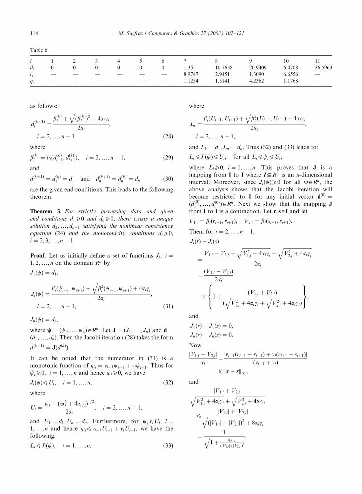
Table 6

i 1 2 3 4 5 6 7 8 9 10 11

di 0 0 0 0 0 0 1.35 10.7658 20.9409 6.4708 36.5963

ri — — — — — — 8.9747 2.9451 1.3090 6.6556 —

qi — — — — — — 1.1254 1.5141 4.2362 1.1768 —


Hence, because of the existence of upper bounds U ’s we

have the following:

jjJðrÞ � JðsÞjjNp1

21þ

1ffiffiffiffiffiffiffiffiffiffiffi1þ l

p( )

jjr� sjjN; ð34Þ

where

l ¼2 mini aigi

ðmaxi;r biðrÞÞ2> 0:

It follows from (34) that J is a contraction mapping on I.

Hence the Jacobi iteration converges to a unique fixed

point d in I, i.e. d ¼ GðdÞ: This d is the unique solution tothe system (24). &

Remark 3. While it is true that a nonlinear quadratic

system may not be as efficient as a linear system

of equations, this computational drawback, is

compensated by the use of a rational quadratic

interpolant (23) instead of a rational cubic (2) through

another interesting feature of the choice of shape

parameters in (22).

Remark 4. It is hoped that the author, in future, will be

able to improve on the numerical technique for resolving

the system of nonlinear Eqs. (24). This work is currently

in progress and will be reported in a future paper.

4. Better accuracy

In this section we establish error bounds for the

rational cubic spline methods of Sections 3 and 4. This

will show that new monotone curve scheme, in Section

4, is superior to the scheme in Section 3 as far as

accuracy is concerned. The main results follows in the

following theorem.

Theorem 4. Let vi;wiXai > �1; fAC4½x1; xn�; and s be

the piecewise rational cubic interpolant function such that

sðxiÞ ¼ f ðxiÞ and sð1ÞðxiÞ ¼ di; i ¼ 1; 2;y; n: Then for

xA½xi; xiþ1� and

bi ¼ð1þ aiÞ=4 if � 1oaio3;

1 if aiX3;

(

jf ðxÞ � sðxÞjphi

4bi

gi þEðf Þ98

�;

where

gi ¼ maxðjf ð1Þi � di j; jf

ð1Þiþ1 � diþ1jÞ;

Eðf Þ ¼ fh3i jjfð4Þjjð1þ jai � 3j=4Þ þ 4jai � 3jðh2l jjf

ð3Þjj

þ 3hi jjf ð2ÞjjÞg;

and the symbol jj:jj denotes the uniform norm.

Proof. The proof of the theorem is highly mathematical

and hence is left to avoid unnecessary length. &

The following result follows directly from the above

Theorem.

Corollary 5. Let xA½xi;xiþ1�; and m ¼ 2; 3; then if gi ¼OðhmÞ; and ai � 3 ¼ Oðhm�1Þ; the error bounds are

achieved as jf ðxÞ � sðxÞj ¼ Oðhmþ1Þ:

Remark 5. It is worth to note that, in Section 4, vi ¼1þ di þ diþ1=Wi ¼ wi: Hence, the choice vi ¼ ai ¼ wi;leads to the following:

ai � 3 ¼ �2þdi þ diþ1

Wi

:

It can be also shown that

ai � 3 ¼ ðdi � fð1Þ

i þ diþ1 � fð1Þ

iþ1Þ=jWi j þ Oðh2i Þ:

Remark 6. The above corollary shows the superiority of

the method of Section 4 over the method of Section 3

with an error bound Oðh2Þ: It can be seen that the error

bound of the method in Section 3 is only Oð1Þ:

5. Demonstrations

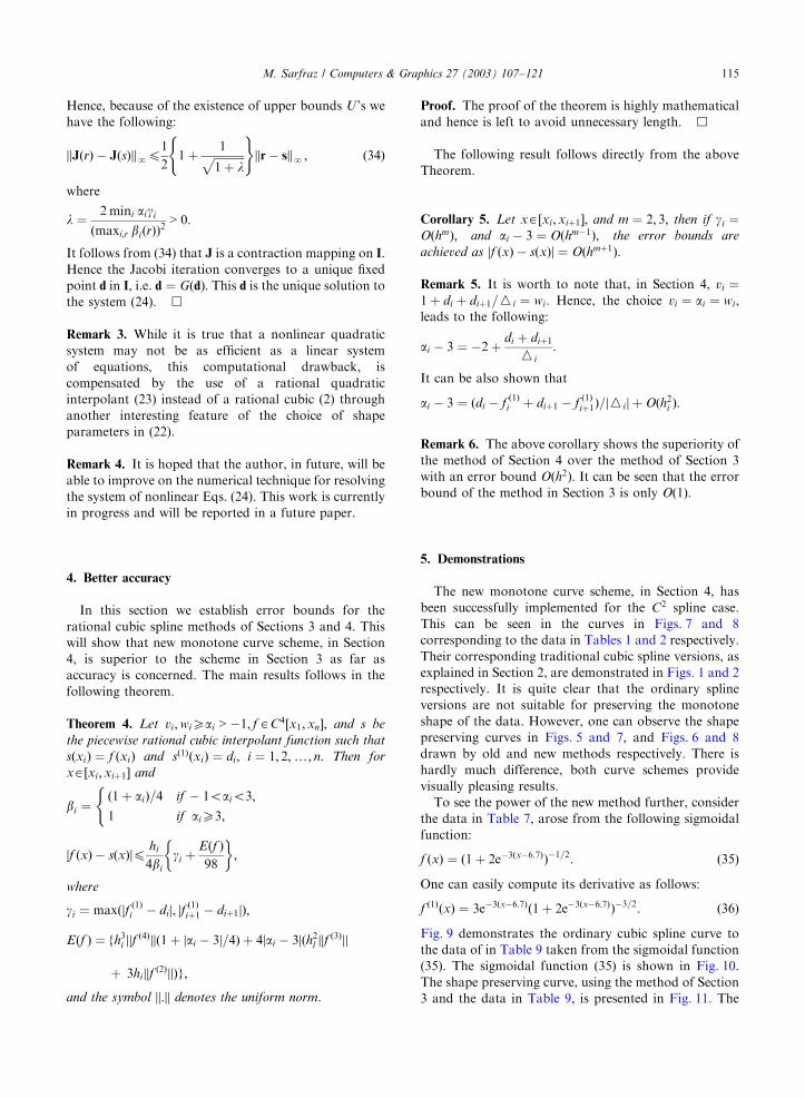
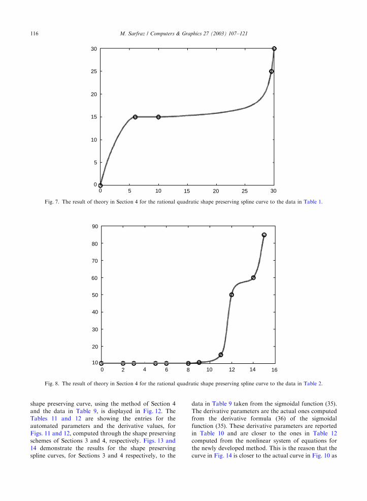
The new monotone curve scheme, in Section 4, has

been successfully implemented for the C2 spline case.

This can be seen in the curves in Figs. 7 and 8

corresponding to the data in Tables 1 and 2 respectively.

Their corresponding traditional cubic spline versions, as

explained in Section 2, are demonstrated in Figs. 1 and 2

respectively. It is quite clear that the ordinary spline

versions are not suitable for preserving the monotone

shape of the data. However, one can observe the shape

preserving curves in Figs. 5 and 7, and Figs. 6 and 8

drawn by old and new methods respectively. There is

hardly much difference, both curve schemes provide

visually pleasing results.

To see the power of the new method further, consider

the data in Table 7, arose from the following sigmoidal

function:

f ðxÞ ¼ ð1þ 2e�3ðx�6:7ÞÞ�1=2: ð35Þ

One can easily compute its derivative as follows:

f ð1ÞðxÞ ¼ 3e�3ðx�6:7Þð1þ 2e�3ðx�6:7ÞÞ�3=2: ð36Þ

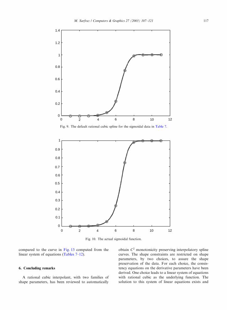
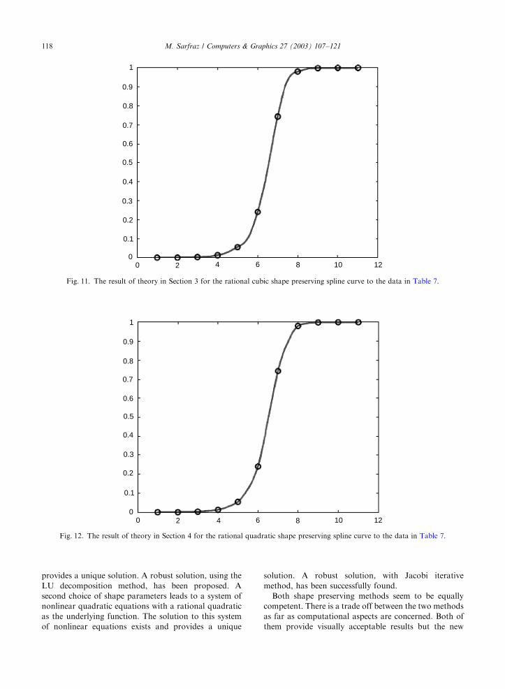
Fig. 9 demonstrates the ordinary cubic spline curve to

the data of in Table 9 taken from the sigmoidal function

(35). The sigmoidal function (35) is shown in Fig. 10.

The shape preserving curve, using the method of Section

3 and the data in Table 9, is presented in Fig. 11. The


shape preserving curve, using the method of Section 4

and the data in Table 9, is displayed in Fig. 12. The

Tables 11 and 12 are showing the entries for the

automated parameters and the derivative values, for

Figs. 11 and 12, computed through the shape preserving

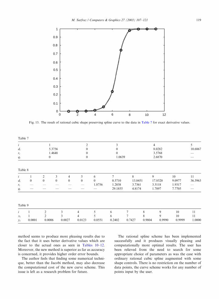
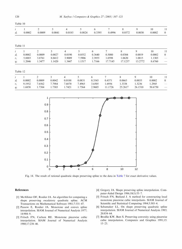
schemes of Sections 3 and 4, respectively. Figs. 13 and

14 demonstrate the results for the shape preserving

spline curves, for Sections 3 and 4 respectively, to the

data in Table 9 taken from the sigmoidal function (35).

The derivative parameters are the actual ones computed

from the derivative formula (36) of the sigmoidal

function (35). These derivative parameters are reported

in Table 10 and are closer to the ones in Table 12

computed from the nonlinear system of equations for

the newly developed method. This is the reason that the

curve in Fig. 14 is closer to the actual curve in Fig. 10 as

30

25

20

15

10

5

00 5 10 15 20 25 30

Fig. 7. The result of theory in Section 4 for the rational quadratic shape preserving spline curve to the data in Table 1.

90

80

70

60

50

40

30

20

100 2 4 6 8 10 12 14 16



compared to the curve in Fig. 13 computed from the

linear system of equations (Tables 7–12).

6. Concluding remarks

A rational cubic interpolant, with two families of

shape parameters, has been reviewed to automatically

obtain C2 monotonicity preserving interpolatory spline

curves. The shape constraints are restricted on shape

parameters, by two choices, to assure the shape

preservation of the data. For each choice, the consis-

tency equations on the derivative parameters have been

derived. One choice leads to a linear system of equations

with rational cubic as the underlying function. The

solution to this system of linear equations exists and

1.4

1.2

1

0.8

0.6

0.4

0.2

00 2 4 6 8 10 12

Fig. 9. The default rational cubic spline for the sigmoidal data in Table 7.

1

0.9

0.8

0.7

0.6

0.5

0.4

0.3

0.2

0.1

00 2 4 6 8 10 12

Fig. 10. The actual sigmoidal function.


provides a unique solution. A robust solution, using the

LU decomposition method, has been proposed. A

second choice of shape parameters leads to a system of

nonlinear quadratic equations with a rational quadratic

as the underlying function. The solution to this system

of nonlinear equations exists and provides a unique

solution. A robust solution, with Jacobi iterative

method, has been successfully found.

Both shape preserving methods seem to be equally

competent. There is a trade off between the two methods

as far as computational aspects are concerned. Both of

them provide visually acceptable results but the new

1

0.9

0.8

0.7

0.6

0.5

0.4

0.3

0.2

0.1

00 2 4 6 8 10 12


1

0.9

0.8

0.7

0.6

0.5

0.4

0.3

0.2

0.1

00 2 4 6 8 10 12



method seems to produce more pleasing results due to

the fact that it uses better derivative values which are

closer to the actual ones as seen in Tables 10–12.

Moreover, the new method is superior as far as accuracy

is concerned, it provides higher order error bounds.

The author feels that finding some numerical techni-

que, better than the Jacobi method, may also decrease

the computational cost of the new curve scheme. This

issue is left as a research problem for future.

The rational spline scheme has been implemented

successfully and it produces visually pleasing and

computationally more optimal results. The user has

been relieved from the need to search for some

appropriate choice of parameters as was the case with

ordinary rational cubic spline augmented with some

shape controls. There is no restriction on the number of

data points, the curve scheme works for any number of

points input by the user.

1

0.9

0.8

0.7

0.6

0.5

0.4

0.3

0.2

0.1

00 2 4 6 8 10 12

Fig. 13. The result of rational cubic shape preserving spline curve to the data in Table 7 for exact derivative values.

Table 7

i 1 2 3 4 5

di 5.3756 0 0 8.0282 10.6867

ri 1.4648 0 0 3.5768 —

qi 0 0 1.0639 2.6870 —

Table 8

i 1 2 3 4 5 6 7 8 9 10 11

di 0 0 0 0 0 0 0.5710 13.8451 17.8520 9.0977 36.5963

ri — — — — — 1.8756 1.2038 3.7361 3.5118 1.9317 —

qi — — — — — — 29.1855 4.8174 1.7897 7.7705 —

Table 9

i 1 2 3 4 5 6 7 8 9 10 11

xi 1 2 3 4 5 6 7 8 9 10 11

yi 0.0001 0.0006 0.0027 0.0123 0.0551 0.2402 0.7427 0.9804 0.9990 0.9999 1.0000


References

[1] McAllister DF, Roulier JA. An algorithm for computing a

shape preserving osculatory quadratic spline. ACM

Transactions on Mathematical Software 1981;7:331–47.

[2] Passow E, Roulier JA. Monotone and convex spline

interpolation. SIAM Journal of Numerical Analysis 1977;

14:904–9.

[3] Fritsch FN, Carlson RE. Monotone piecewise cubic

interpolation. SIAM Journal of Numerical Analysis

1980;17:238–46.

[4] Gregory JA. Shape preserving spline interpolation. Com-

puter-Aided Design 1986;18(1):53–7.

[5] Fritsch FN, Butland J. A method for constructing local

monotone piecewise cubic interpolants. SIAM Journal of

Scientific and Statistical Computing 1984;5:303–4.

[6] Schumaker LL. On shape preserving quadratic spline

interpolation. SIAM Journal of Numerical Analysis 1983;

20:854–64.

[7] Brodlie KW, Butt S. Preserving convexity using piecewise

cubic interpolation. Computers and Graphics 1991;15:

15–23.

Table 10

i 1 2 3 4 5 6 7 8 9 10 11

di 0.0002 0.0009 0.0041 0.0185 0.0824 0.3395 0.4996 0.0572 0.0030 0.0002 0

Table 11

i 1 2 3 4 5 6 7 8 9 10 11

di 0.0002 0.0009 0.0027 0.0190 0.0552 0.3640 0.5080 0.0304 0.0019 0.0002 0

ri 5.8885 3.8761 8.0412 3.9009 7.5906 2.3955 1.0598 1.0620 1.0815 1.1303 —

qi 1.2046 1.3477 1.1420 1.3447 1.1517 1.7166 17.7145 17.1237 13.2772 8.6760 —

Table 12

i 1 2 3 4 5 6 7 8 9 10 11

di 0.0002 0.0009 0.0042 0.0188 0.0831 0.3545 0.4371 0.0663 0.0035 0.0002 0

ri 9.1952 7.6562 7.7984 7.6870 7.4965 3.6505 1.6956 1.3338 1.3236 1.2945 —

qi 1.6858 1.7384 1.7303 1.7421 1.7564 2.9605 11.1726 25.2617 26.1510 50.6750 —

1

0.9

0.8

0.7

0.6

0.5

0.4

0.3

0.2

0.1

00 2 4 6 8 10 12

Fig. 14. The result of rational quadratic shape preserving spline to the data in Table 7 for exact derivative values.


[8] Sarfraz M. Convexity preserving piecewise rational inter-

polation for planar curves. Bulletin of the Korean

Mathematical Society 1992;29(2):193–200.

[9] Sarfraz M. Preserving Monotone shape of the Data using

Piecewise Rational Cubic Functions. Computers and

Graphics 1997;21(1):5–14.

[10] Brodlie KW. Methods for drawing curves. In: Earnshaw

RA, editor. Fundamental algorithm for computer

graphics. Berlin: Springer, 1985. p. 303–23.

[11] DeVore A, Yan Z. Error analysis for piecewise quadratic

curve fitting algorithms. Computer Aided Geometric

Design 1986;3:205–15.

[12] Greiner K. A survey on univariate data interpolation and

approximation by splines of given shape. Mathematical

and Computer Modelling 1991;15:97–106.

[13] Constantini P. Boundary-valued shape preserving inter-

polating splines. ACM Transactions on Mathematical

Software 1997;23(2):229–51.

[14] Lahtinen A. Monotone interpolation with application to

estimation of taper curves. Annals of Numerical Mathe-

matics 1996;3:151–61.

[15] Sarfraz M. Interpolatory rational cubic spline with biased,

point and interval tension. Computers and Graphics

1992;16(4):427–30.

[16] Sarfraz M. A rational cubic spline for the visualization of

monotonic data. Computers and Graphics 2000;24(4):509–16.

[17] Press WH, Teukolsky SA, Vetterling WT, Flannery BP.

Numerical recipes in C: The art of scientific computing.

Cambridge: Cambridge University Press, 1992.

[18] Press WH, Teukolsky SA, Vetterling WT, Flannery BP.

Numerical recipes in Fortran 90: The art of parallel

scientific computing. Cambridge: Cambridge University

Press, 1996.

[19] Sarfraz M. Some remarks on a rational cubic spline for the

visualization of monotonic data. Computers and Graphics

2002;26(1):193–7.


Documents

A rational cubic spline for the visualization of monotonic data: an alternate approach