Embed Size (px)
Citation preview

Logical Methods in Computer Science
Vol. 14(1:10)2018, pp. 1–27
https://lmcs.episciences.org/
Submitted Jun. 12, 2017
Published Jan. 23, 2018
A REAL-VALUED MODAL LOGIC
DENISA DIACONESCU a, GEORGE METCALFE b, AND LAURA SCHNURIGER c
a Faculty of Mathematics and Computer Science, University of Bucharest, Romaniae-mail address: [email protected]
b,c Mathematical Institute, University of Bern, Switzerlande-mail address: george.metcalfe,[email protected]
Abstract. A many-valued modal logic is introduced that combines the usual Kripkeframe semantics of the modal logic K with connectives interpreted locally at worlds bylattice and group operations over the real numbers. A labelled tableau system is providedand a coNEXPTIME upper bound obtained for checking validity in the logic. Focussingon the modal-multiplicative fragment, the labelled tableau system is then used to establishcompleteness for a sequent calculus that admits cut-elimination and an axiom system thatextends the multiplicative fragment of Abelian logic.
1. Introduction
Many-valued modal logics combine the frame semantics of classical modal logics with amany-valued semantics at each world. As in the classical case, they may be understood as acompromise between the good computational properties (decidability and lower complexity)of propositional logics and the expressivity of their first-order counterparts, some of whichare not even recursively axiomatizable. Such logics have been used to model modal notionssuch as necessity, belief, and spatio-temporal relations in the presence of multiple degrees oftruth, certainty, and possibility, and span fuzzy belief [19, 15], fuzzy similarity measures [16],many-valued tense logics [20, 11], and spatial reasoning with vague predicates [33]. Theyalso provide a basis for studying fuzzy description logics, which, analogously to the classicalcase, may be understood as many-valued multi-modal logics (see, e.g., [34, 18, 23, 1]).
Uniform approaches to many-valued modal logics defined over algebras with a completelattice reduct are described in [5, 32], extending previous work on modal logics based on
Key words and phrases: Many-Valued Logic, Modal Logic, Abelian Logic, Lukasiewicz Logic, Proof The-ory, Tableau Calculus, Sequent Calculus.
A precursor to this paper, reporting preliminary results, appeared in the proceedings of AiML 2016 [12].The research of the first author was supported by Sciex grant 13.192 and Romanian National Authority
for Scientific Research and Innovation grant, CNCS-UEFISCDI, project number PN-II-RU-TE-2014-4-0730.The second and third authors acknowledge support from Swiss National Science Foundation grant
200021 146748 and the EU Horizon 2020 research and innovation programme under the Marie Sk lodowska-Curie grant agreement No 689176.
LOGICAL METHODSl IN COMPUTER SCIENCE DOI:10.23638/LMCS-14(1:10)2018
c© D. Diaconescu, G. Metcalfe, and L. SchnürigerCC© Creative Commons

2 D. DIACONESCU, G. METCALFE, AND L. SCHNURIGER
finite Heyting algebras [13, 14]. In an infinite-valued setting, two core families emerge:“order-based” modal logics, including modal extensions of Godel logics [7, 28, 8, 6], whereonly the order type of the truth values matters, and “continuous” modal logics, such asthose based on Lukasiewicz logic [17, 5, 21, 25, 26, 3], where propositional connectives areinterpreted by continuous functions over sets of real numbers (see also [24, 23, 27] for relatedsystems). Such logics are easy to define semantically — just decide on a suitable set of valuesand operations — but not so easy to study. For example, an axiomatization for the Godelmodal logic over many-valued frames is provided in [8], but no axiomatization is yet knownfor the Godel modal logic over standard (Boolean-valued or “crisp”) frames. Moreover,decidability and complexity problems for these and other order-based modal logics, whichtypically lack the finite model property, have been solved only recently (see [6]).
In this paper we focus on continuous modal logics. Axiomatizations for finite-valued Lukasiewicz modal logics have been provided in [21], but the axiom system presented for theinfinite-valued Lukasiewicz modal logic K(Ł) includes a rule with infinitely many premises.Similarly, only an approximate completeness result (corresponding to including an infinitaryrule) is established for the closely related continuous propositional modal logic consideredin [3]. Studying logics that lack a finitary axiom system, and therefore also a suitablealgebraic semantics, may be difficult, as may be seen by considering classical modal logicdeprived of the theory of Boolean algebras with operators. Note also that, although validityin finite-valued Lukasiewicz modal logics is PSPACE-complete [4], only a coNEXPTIMEupper bound is known for the infinite-valued case, as may be deduced from complexityresults for Lukasiewicz description logics (see [23]).
We address some of these issues here by defining and investigating a many-valuedmodal logic K(A) with propositional connectives interpreted as the usual lattice and groupoperations over the real numbers. According to this semantics, the logic may be viewedas a minimal modal extension of Abelian logic, the logic of lattice-ordered abelian groups,introduced independently by Meyer and Slaney as a relevant logic [31] and Casari as acomparative logic [9]. Some refinements to the usual definition of many-valued modal logics(see, e.g., [5]) are needed to deal with the fact that the real numbers do not form a completelattice. However, since K(A) enjoys a finite model property, these non-standard featurescan be safely ignored for practical purposes. Indeed, the logic K(A) provides a rather simpleformalism for reasoning about state transition systems where linear combinations of real-valued variables are compared among worlds using modal operators. Since the connectivesare interpreted by common arithmetical operations min, max, +, and −, further connectivesinterpreted by combinations of these operations (e.g., for many-valued modal or descriptionlogics that reason about degrees of truth, certainty, and possibility) can also be defined inthis setting. In particular, we show here that the Lukasiewicz modal logic K(Ł) can beinterpreted in the logic K(A) extended with a constant.
As our first main technical contribution, we present a sound and complete labelledtableau calculus for K(A) and obtain a coNEXPTIME upper bound for checking va-lidity in this logic. The calculus is quite closely related to a labelled tableau calculusfor a Lukasiewicz description logic presented in [23], and indeed provides the same upperbound for checking validity. However, an important advantage of defining a logic overlattice-ordered abelian groups is that we are able to explicitly identify and study the modal-multiplicative fragment, solving problems for this fragment that seem at the moment tobe quite difficult for the full logic. In particular, we show that the modal-multiplicativefragment of K(A) has an EXPTIME upper bound for checking validity and provide a

A REAL-VALUED MODAL LOGIC 3
sequent calculus for the fragment that admits cut-elimination. More significantly, we usethe labelled tableau calculus to establish the completeness of an axiom system extendingthe multiplicative fragment of Abelian logic that, unlike other known axiomatizations forcontinuous modal logics, contains only finitary rules.
2. A Modal Extension of Abelian Logic
In this section we define the real-valued modal logic K(A) semantically as a minimal modalextension of Abelian logic A, the logic of lattice-ordered abelian groups. We then showthat validity in this logic remains unchanged when the semantics is restricted to the classof finite serial models. Finally, we provide a syntactic embedding of the minimal modalextension K(Ł) of infinite-valued Lukasiewicz logic into K(A) with an additional constant.
Since we will consider several propositional languages in this paper, let us begin withsome quite general definitions. Given a propositional language L (also known as an algebraicsignature or type) consisting of connectives with fixed arities, let Fm(L) denote the set ofL-formulas ϕ,ψ, χ, . . . , defined inductively in the usual way over a countably infinite setVar of (propositional) variables p, q, r, . . . . The complexity of ϕ ∈ Fm(L) is the number ofoccurrences of connectives in ϕ, and if L contains a unary operation , then the modaldepth of ϕ is the deepest nesting of the modal connective in ϕ.
2.1. Abelian Logic. Let us begin with a brief summary of Abelian logic A, introducedindependently by Meyer and Slaney in [31] as a relevant logic, and Casari in [9] as acomparative logic. In both settings, A was defined via axiom systems that are completewith respect to validity in the variety of lattice-ordered abelian groups. However, since thisvariety is generated by a single algebra defined over the real numbers, we may also use thisalgebra to introduce Abelian logic semantically as a many-valued logic.
Consider a language LA with binary connectives ∧, ∨, &, and →, and a constant0, fixing also ¬ϕ := ϕ → 0. We define Abelian logic A via the logical matrix 〈R,R+
0 〉consisting of the algebra R = 〈R,min,max,+,−, 0〉 and the set of designated truth valuesR+0 = r ∈ R : r ≥ 0. That is, an A-valuation is a map e : Var → R extended to all
LA-formulas bye(ϕ ∧ ψ) = min(e(ϕ), e(ψ))
e(ϕ ∨ ψ) = max(e(ϕ), e(ψ))
e(ϕ&ψ) = e(ϕ) + e(ψ)
e(ϕ → ψ) = e(ψ) − e(ϕ)
e(0) = 0,
and ϕ ∈ Fm(LA) is A-valid if e(ϕ) ≥ 0 for each A-valuation e.As mentioned above, R generates the variety of lattice-ordered abelian groups. But
also, using methods of abstract algebraic logic, it is easily proved that this variety providesan algebraic semantics for the axiom system HA displayed in Figure 1: an axiomatizationof multiplicative additive intuitionistic linear logic with just one constant 0 extended withthe axiom schema (A) ((ϕ → ψ) → ψ) → ϕ. It follows then that ϕ ∈ Fm(LA) is derivablein HA if and only if ϕ is A-valid.
The choice of Abelian logic as the basis for the many-valued modal logics studied in thispaper is motivated both by its expressivity and the central role of its semantics in ordinarymathematics. The connectives of A are interpreted by the basic arithmetical operations

4 D. DIACONESCU, G. METCALFE, AND L. SCHNURIGER
(B) (ϕ→ ψ) → ((ψ → χ) → (ϕ→ χ))(C) (ϕ→ (ψ → χ)) → (ψ → (ϕ→ χ))( I ) ϕ→ ϕ
(A) ((ϕ → ψ) → ψ) → ϕ
(&1) ϕ→ (ψ → (ϕ&ψ))(&2) (ϕ→ (ψ → χ)) → ((ϕ&ψ) → χ)(0 1) 0(0 2) ϕ→ (0 → ϕ)(∧1) (ϕ ∧ ψ) → ϕ
(∧2) (ϕ ∧ ψ) → ψ
(∧3) ((ϕ → ψ) ∧ (ϕ→ χ)) → (ϕ→ (ψ ∧ χ))(∨1) ϕ→ (ϕ ∨ ψ)(∨2) ψ → (ϕ ∨ ψ)(∨3) ((ϕ → χ) ∧ (ψ → χ)) → ((ϕ ∨ ψ) → χ)
ϕ ϕ→ ψ
ψ(mp)
ϕ ψ
ϕ ∧ ψ(adj)
Figure 1: The Axiom System HA
min, max, +, −, and 0, from which connectives for other many-valued logics, interpretedvia combinations of these operations, can be defined. In particular, there exist syntacticembeddings of infinite-valued Lukasiewicz logic into A that allow results for the latter tobe transferred to results about the former. The use of basic arithmetical operations on thereal numbers means also that a huge array of results and methods from linear algebra areavailable for investigating A and its modal expansions. For example, such methods havebeen used to obtain analytic sequent and hypersequent calculi and co-NP completenessresults for Abelian logic and infinite-valued Lukasiewicz logic in [29] (see also [2, 30]).
2.2. Kripke Semantics. We define a minimal (crisp) modal extension K(A) of Abelianlogic by interpreting formulas locally in the algebra R over standard Kripke frames. That is,a (crisp) frame is a pair F = 〈W,R〉, where W is a non-empty set of worlds and R ⊆W ×Wis an (crisp) accessibility relation. As usual, we write Rxy or Rxy = 1 to denote 〈x, y〉 ∈ R
and Rxy = 0 to denote 〈x, y〉 6∈ R. For any x ∈ W , we let R[x] = y ∈ W : Rxy. Modalformulas are defined over the language L
A extending LA with an additional unary “box”connective , where the dual “diamond” connective is defined as ♦ϕ := ¬¬ϕ.
There exists a very general method for defining crisp modal logics over algebras with acomplete lattice reduct (see in particular [5]), where the and ♦ connectives are interpretedas infima and suprema of values of formulas at accessible worlds. However, since the realnumbers do not form a complete lattice — they lack a top and bottom element — we makehere a couple of minor adjustments to this method. First, we adopt the useful conventionthat
∧
R∅ =
∨
R∅ = 0, and second, we restrict valuations of variables in a particular model
to a fixed interval. Both these choices will be justified to some extent by Lemma 2.1 below.

A REAL-VALUED MODAL LOGIC 5
A K(A)-model M = 〈W,R, V 〉 consists of a frame 〈W,R〉 together with a valuation mapV : Var ×W → [−r, r] for some r ∈ R
+0 that is extended to V : Fm(L
A) ×W → R by
V (ϕ ∧ ψ, x) = min(V (ϕ, x), V (ψ, x))
V (ϕ ∨ ψ, x) = max(V (ϕ, x), V (ψ, x))
V (ϕ&ψ, x) = V (ϕ, x) + V (ψ, x)
V (ϕ→ ψ, x) = V (ψ, x) − V (ϕ, x)
V (0, x) = 0
V (ϕ, x) =∧
RV (ϕ, y) : Rxy.
By calculation, we obtain also
V (¬ϕ, x) = −V (ϕ, x)
V (♦ϕ, x) =∨
RV (ϕ, y) : Rxy.
An LA-formula ϕ is valid in a K(A)-model M = 〈W,R, V 〉 if V (ϕ, x) ≥ 0 for all x ∈ W . If
ϕ is valid in all K(A)-models, then ϕ is K(A)-valid, written |=K(A) ϕ.The convention that
∧
R∅ =
∨
R∅ = 0 is rather counter-intuitive. This can be avoided,
however, by restricting to serial frames: that is, frames F = 〈W,R〉 such that for all x ∈W ,there exists y ∈W such that Rxy. With this restriction,
∧
R∅ and
∨
R∅ may simply be left
undefined. Similarly, restricting the codomain of a valuation to a bounded subset of R canbe avoided by considering only finite models. Surprisingly perhaps, considering only finiteserial models does not affect the valid formulas of the logic.
Lemma 2.1. |=K(A) ϕ if and only if ϕ is valid in all finite serial K(A)-models.
Proof. The left-to-right direction is immediate. For the opposite direction, we note firstthat if ϕ is not valid in a K(A)-model M = 〈W,R, V 〉, then it will not be valid in the serialK(A)-model M′ = 〈W ∪W ′, R∪R′, V ′〉 where W ′ is a set of new distinct worlds x′ for eachx ∈ W satisfying R[x] = ∅, R′ = 〈x, x′〉, 〈x′, x′〉 : x ∈ W and R[x] = ∅, and V ′ extends Vwith V (p, x′) = 0 for all p ∈ Var and x′ ∈W ′. Clearly, if M is finite, then M′ is also finite.
It now suffices to prove the following: for any K(A)-model M = 〈W,R, V 〉, x ∈ W ,finite set of formulas S, and ε > 0, there exists a finite K(A)-model M′ = 〈W ′, R′, V ′〉 withx ∈ W ′ such that |V (ϕ, x) − V ′(ϕ, x)| < ε for all ϕ ∈ S. We proceed by induction on thesum of the complexities of the formulas in S.
For the base case, S contains only variables and 0, and we let M′ = 〈W ′, R′, V ′〉 withW ′ = x, R′ = ∅, and V ′(p, x) = V (p, x) for each p ∈ Var. For the inductive step, supposefirst that S = S′ ∪ ψ1 → ψ2. Then we can apply the induction hypothesis with M,x ∈ W , S′′ = S′ ∪ ψ1, ψ2, and ε
2 > 0 to obtain a finite K(A)-model M′ = 〈W ′, R′, V ′〉with x ∈ W ′ such that |V (ϕ, x) − V ′(ϕ, x)| < ε
2 for all ϕ ∈ S′′. It suffices then to observethat |V (ψ1 → ψ2, x) − V ′(ψ1 → ψ2, x)| = |V (ψ2, x) − V (ψ1, x) − V ′(ψ2, x) + V ′(ψ1, x)| ≤|V (ψ2, x) − V ′(ψ2, x)| + |V (ψ1, x) − V ′(ψ1, x)| < ε
2 + ε2 = ε. The cases where S contains
ψ1&ψ2, ψ1 ∧ ψ2, or ψ1 ∨ ψ2 are very similar.Finally, suppose that S consists of variables and boxed formulas ψ1, . . . ,ψn (n ≥ 1).
Then for i ∈ 1, . . . , n, there exists yi ∈W such that Rxyi and |V (ψi, x)−V (ψi, yi)| <ε2 .
We apply the induction hypothesis to each submodel Mi of M generated by yi (i.e., therestriction of M to the smallest subset of W containing yi and closed under R) with S′ =(S \ ψ1, . . . ,ψn) ∪ ψ1, . . . , ψn, yi ∈ Wi, and ε
2 > 0 to obtain a finite K(A)-modelM′
i = 〈W ′i , R
′i, V
′i 〉 and yi ∈ W ′
i such that |V (ϕ, yi) − V ′(ϕ, yi)| <ε2 for all ϕ ∈ S′. By
renaming worlds, we may assume that these models are disjoint and do not include x. Now

6 D. DIACONESCU, G. METCALFE, AND L. SCHNURIGER
let M′ = 〈W ′, R′, V ′〉 be the finite K(A)-model with W ′ = x ∪W ′1 ∪ . . . ∪W
′n such that
for u, v ∈W ′ and p ∈ Var,
R′uv =
R′iuv if u, v ∈W ′
i
1 if u = x, v ∈ y1, . . . , yn
0 otherwise
and V ′(p, u) =
V ′i (p, u) if u ∈W ′
i
V (p, x) if u = x.
Clearly V ′(p, x) = V (p, x) for each variable p ∈ S. Moreover, |V (ψi, x) − V (ψi, yi)| <ε2
and |V (ψi, yj) − V ′(ψi, yj)| <ε2 for i, j ∈ 1, . . . , n, so |V (ψi, x) − V ′(ψi, x)| < ε.
As remarked above, the preceding lemma provides some justification both for assumingin the definition of the semantics of K(A) that
∧
R∅ =
∨
R∅ = 0, and for restricting
valuations of variables in a particular K(A)-model to a fixed interval. It shows that fordetermining the valid formulas of K(A), we need only consider finite serial K(A)-models.For such frames we can leave
∧
R∅ and
∨
R∅ undefined; we can also make use of a standard
(unrestricted) valuation map V : Var ×W → R, since only finite infima and suprema areneeded for calculating values of formulas. In principle then, we could define the logic K(A)without extra assumptions by considering only finite serial K(A)-models. We prefer here,however, to give a more general semantics and to discover this finite model property as afact about the logic rather than building it into the definition.
Example 2.2. Any K(A)-model can be viewed as a state transition system, where eachstate is labelled with a vector of real numbers that represents the values of the variables inVar at that state. Such a transition system may be used to represent choices for variousplayers in a game together with points (or other resources) accumulated by the playersduring that game. Consider for example the K(A)-model M = 〈W,R, V 〉 depicted below,
where the vectors(
p
q
)
represent the values of p and q, respectively, at each state.
(
00
)
(
10
) (
01
)
(
20
) (
41
) (
11
) (
13
)
We can use the model M to define various two-player games, where in the first round,starting at the root, Player P chooses one of several (in this case, two) options, and in thesecond round, Player Q also chooses one of several (in this case, also two) options. Thepoints assigned to Player P and Player Q at each state are the values of p and q, respectively.Let also call the values of p − q and q − p at a state, the scores for P and Q, respectively.We assume in all these games that the players have complete knowledge of both M andtheir opponent’s goals.
Let us consider some different ways of concluding games based on M. Suppose that inGame 1 each player’s goal is to maximize her final score. Player P ’s maximal payoff is thenthe value at the root of the formula ♦(q → p), which is 2. If Player P ’s goal in Game 2 is

A REAL-VALUED MODAL LOGIC 7
to maximize her final number of points, and Player Q aims to minimize this number, thenthe required formula is ♦p, which at the root also takes value 2. Reversing the roles forGame 3, we obtain the formula ♦q, which takes value 1 at the root. More complicatedgoals can also be modelled. For example, if both players aim to maximize the sum of theirscores accumulated during the two rounds, then Player P ’s maximal payoff is the value ofthe formula ♦((q → p)&(q → p)) at the root, namely 3.
Formulas can also be used to express general relationships between games. For example,the model M shows that
6|=K(A) ♦(q → p) → (♦q → ♦p).
That is, Player P ’s maximal payoff in Game 1 exceeds her maximal payoff in Game 2 minusher maximal payoff in Game 3. On the other hand, it can be shown (e.g., using one of thecalculi introduced below) that
|=K(A) ♦(q → p) → (q → ♦p).
This means that if the goals of Games 1 and 2 are adopted with respect to an arbitraryK(A)-model M′ based on a finite rooted tree with branches of length 2, then Player P ’smaximal payoff in Game 1 for M′ is always less than or equal to her maximal payoff inGame 2 for M′ minus the minimum number of points for Player Q in all final states of M′.
2.3. Lukasiewicz Modal Logic. Let us briefly recall the semantics of the Lukasiewiczmodal logic K(Ł) studied by Hansoul and Teheux in [21]. For convenience, we make use ofa language L
Łwith the binary connective ⊃ and unary connectives ∼ and , where further
connectives are defined as ϕ⊕ψ := ∼ϕ ⊃ ψ, ϕ⊙ψ := ∼(∼ϕ⊕∼ψ), ϕ∨ψ := (ϕ ⊃ ψ) ⊃ ψ,ϕ ∧ ψ := ∼(∼ϕ ∨ ∼ψ), and ♦ϕ := ∼∼ϕ.
A K(Ł)-model M = 〈W,R, V 〉 consists of a frame 〈W,R〉 and a valuation map V : Var×W → [0, 1] that is extended to V : Fm(L
Ł) ×W → [0, 1] by
V (∼ϕ, x) = 1 − V (ϕ, x)
V (ϕ ⊃ ψ, x) = min(1, 1 − V (ϕ, x) + V (ψ, x))
V (ϕ, x) =∧
[0,1]V (ϕ, y) : Rxy.
An LŁ
-formula ϕ is valid in a K(Ł)-model M = 〈W,R, V 〉 if V (ϕ, x) = 1 for all x ∈ W . Ifϕ is valid in all K(Ł)-models, then ϕ is K(Ł)-valid, written |=K(Ł) ϕ.
An axiom system for K(Ł) is presented in [21] as an extension of an axiomatization ofinfinite-valued Lukasiewicz logic with the modal axioms and rules
(ϕ ⊃ ψ) ⊃ (ϕ ⊃ ψ)
(ϕ⊕ ϕ) ⊃ (ϕ⊕ϕ)
(ϕ⊙ ϕ) ⊃ (ϕ⊙ϕ)
ϕ
ϕ
and the following rule with infinitely many premises
ϕ⊕ ϕ ϕ⊕ (ϕ ⊙ ϕ) ϕ⊕ (ϕ⊙ ϕ⊙ ϕ) . . .ϕ

8 D. DIACONESCU, G. METCALFE, AND L. SCHNURIGER
It is proved that an LŁ
-formula ϕ is derivable in this system if and only if |=K(Ł) ϕ.1
This raises an intriguing question. Is there an elegant axiomatization containing onlyfinitary rules, obtained perhaps by removing the infinitary rule above? Our first step towardsaddressing this issue will be to view Lukasiewicz modal logic K(Ł) as a fragment of a modestextension of the Abelian modal logic K(A). Let L
Ac be the language LA extended with an
extra constant c. A K(Ac)-model M = 〈W,R, V, cM〉 consists of a K(A)-model 〈W,R, V 〉and an element cM ∈ R, where valuations are extended as before, using the additional clauseV (c, x) = cM for each x ∈W .
Let us fix ⊥ := c ∧ ¬c and define the following mapping from Fm(LŁ
) to Fm(LAc):
p∗ = (p ∧ 0) ∨ ⊥ for each p ∈ Var
(∼ϕ)∗ = ϕ∗ → ⊥
(ϕ ⊃ ψ)∗ = (ϕ∗ → ψ∗) ∧ 0
(ϕ)∗ = ϕ∗.
We show that this mapping preserves validity between K(Ł) and K(Ac) by identifying thevalue taken by an L
Ł-formula in [0, 1] with the value taken by the corresponding L
Ac-formulain the interval [−|c|, 0].
Proposition 2.3. Let ϕ ∈ Fm(LŁ
). Then |=K(Ł) ϕ if and only if |=K(Ac) ϕ∗.
Proof. Suppose first that ϕ is not valid in a K(Ł)-model M = 〈W,R, V 〉. So V (ϕ, x) < 1 forsome x ∈W . We consider the K(Ac)-model M′ = 〈W,R, V ′, cM〉 where V ′(p, x) = V (p, x)−1for any p ∈ Var and x ∈W , and cM = −1. It suffices to prove that V ′(ψ∗, x) = V (ψ, x) − 1for any ψ ∈ Fm(L
Ł), since then V ′(ϕ∗, x) = V (ϕ, x)−1 < 0 and 6|=K(Ac) ϕ
∗. We proceed byinduction on the complexity of ψ. The base case follows by definition and for the inductivestep for the propositional connectives, we just notice that, using the induction hypothesis,
V ′((ψ1 ⊃ ψ2)∗, x) = V ′((ψ∗1 → ψ∗
2) ∧ 0, x)
= min(V ′(ψ∗2 , x) − V ′(ψ∗
1 , x), 0)
= min((V (ψ2, x) − 1) − (V (ψ1, x) − 1), 0)
= min(V (ψ2, x) − V (ψ1, x), 0)
= min(1 − V (ψ1, x) + V (ψ2, x), 1) − 1
= V (ψ1 ⊃ ψ2, x) − 1,
the case where ψ is ∼ψ1 being very similar. For the modal case, we obtain
V ′((ψ1)∗, x) = V ′(ψ∗1 , x)
=∧
RV ′(ψ∗
1 , y) : Rxy
=∧
RV (ψ1, y) − 1 : Rxy
=∧
[0,1]V (ψ1, y) : Rxy − 1
= V (ψ1, x) − 1,
noting that in the case where R[x] = ∅, we obtain∧
RV ′(ψ∗
1 , y) : Rxy = 0 = 1 − 1 =∧
[0,1]V (ψ1, y) : Rxy − 1 as required.
1In fact, the authors of [21] prove a more general strong completeness result: an LŁ -formula ϕ is derivable
from a (possibly infinite) set of LŁ -formulas Σ in the system if and only if for every K(Ł)-model 〈W,R,V 〉
and x ∈W , whenever V (ψ, x) = 1 for all ψ ∈ Σ, also V (ϕ, x) = 1. Note that an infinitary rule is needed toobtain a strong completeness theorem even for propositional Lukasiewicz logic and Abelian logic. However,in this paper we establish only (weak) completeness results.

A REAL-VALUED MODAL LOGIC 9
Suppose now conversely that ϕ∗ is not valid in a K(Ac)-model M = 〈W,R, V, cM〉. Thatis, V (ϕ∗, x) < 0 for some x ∈W . Observe first that if cM = 0, then, by a simple induction onthe complexity of ϕ, we obtain V (ϕ∗, x) = 0 for all x ∈W , a contradiction. Hence cM 6= 0.Moreover, by scaling (dividing V (p, x) by cM for each p ∈ Var and x ∈W ), we may assumethat V (⊥, x) = −1 for all x ∈ W . We consider the K(Ł)-model M′ = 〈W,R, V ′〉 whereV ′(p, x) = max(min(V (p, x)+1, 1), 0). It then suffices to prove that V ′(ψ, x) = V (ψ∗, x)+1for any ψ ∈ Fm(L
Ł), proceeding by induction on the complexity of ψ.
Note that the addition of a constant c to K(A) does not affect the fact that validity inthe logic is equivalent to validity in finite models. It does, however, introduce a differencebetween the logic K(Ac) and the same logic restricted to serial models. Clearly, the formulac→ c is valid in all serial models, but not in all models.
3. A Labelled Tableau Calculus
In this section we introduce a labelled tableau calculus for checking K(A)-validity that isbased very closely on the Kripke semantics described above. We use the calculus here toshow that the problem of checking K(A)-validity is in the complexity class coNEXPTIME.In Section 4, we will also use (a fragment of) the calculus to establish the completeness of anaxiom system and a sequent calculus admitting cut-elimination for the modal-multiplicativefragment of K(A).
3.1. The Calculus. Our labelled tableau calculus LK(A) proves that an LA-formula ϕ is
valid by showing that the assumption that ϕ takes a value less than 0 in some world w1
leads to a contradiction. Informally, we build a tableau for ϕ as follows. First we decomposethe propositional structure of ϕ to obtain inequations between sums of formulas labelledwith the world w1. We then use box formulas occurring on the right of these inequationsto generate new worlds accessible to w1 and further inequations between sums of formulaslabelled with w1 and these accessible worlds. Box formulas on the left are decomposed byconsidering accessible worlds to w1 and generating new inequations for those worlds. Theprocess is then repeated with the new inequations and worlds appearing on the tableau.The formula ϕ will be valid if the generated set of inequations (suitably interpreted) oneach branch of the tableau is unsatisfiable over the real numbers.
By a labelled formula we mean an ordered pair consisting of an LA-formula ϕ and a
natural number k, written (ϕ)k. Given a multiset of LA-formulas Γ = [ϕ1, . . . , ϕn] (denoting
the empty multiset by []) and k1, . . . , kn ∈ N, we let (Γ)k denote the multiset of labelledformulas [(ϕ1)k1 , . . . , (ϕn)kn ].
Tableaux are constructed from (tableau) nodes of two types:
(1) labelled inequations of the form (Γ)k ⊲ (∆)l where ⊲ ∈ >,≥ and (Γ)k, (∆)l are finitemultisets of labelled formulas;
(2) relations of the form rij where i, j ∈ N.
An LK(A)-tableau is a finite tree of nodes generated according to the inference rules of thesystem presented in Figure 2. That is, if nodes above the line in an instance of a ruleoccur on the same branch B, then B can be extended with the nodes below the line. Forconvenience, we often write branches as (numbered) lists, noting for future reference that
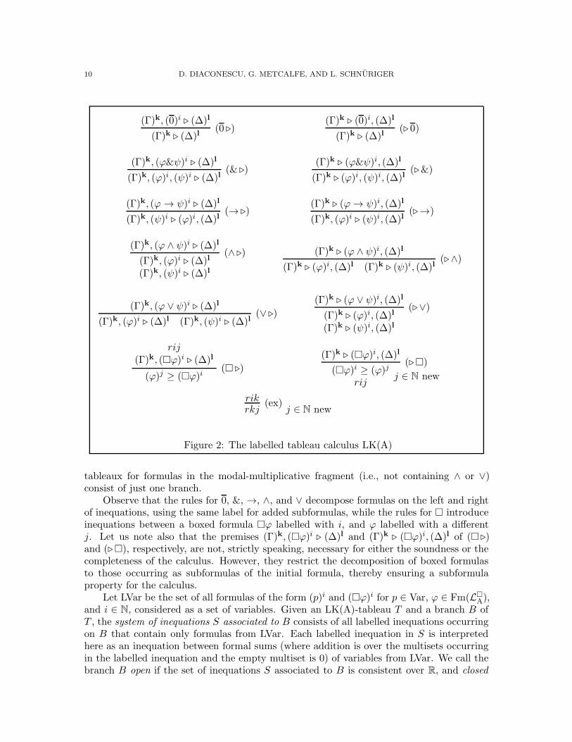
10 D. DIACONESCU, G. METCALFE, AND L. SCHNURIGER
(Γ)k, (0)i ⊲ (∆)l
(Γ)k ⊲ (∆)l(0 ⊲)
(Γ)k ⊲ (0)i, (∆)l
(Γ)k ⊲ (∆)l(⊲ 0)
(Γ)k, (ϕ&ψ)i ⊲ (∆)l
(Γ)k, (ϕ)i, (ψ)i ⊲ (∆)l(& ⊲)
(Γ)k ⊲ (ϕ&ψ)i, (∆)l
(Γ)k ⊲ (ϕ)i, (ψ)i, (∆)l(⊲&)
(Γ)k, (ϕ → ψ)i ⊲ (∆)l
(Γ)k, (ψ)i ⊲ (ϕ)i, (∆)l(→ ⊲)
(Γ)k ⊲ (ϕ→ ψ)i, (∆)l
(Γ)k, (ϕ)i ⊲ (ψ)i, (∆)l(⊲→)
(Γ)k, (ϕ ∧ ψ)i ⊲ (∆)l
(Γ)k, (ϕ)i ⊲ (∆)l
(Γ)k, (ψ)i ⊲ (∆)l
(∧ ⊲) (Γ)k ⊲ (ϕ ∧ ψ)i, (∆)l
(Γ)k ⊲ (ϕ)i, (∆)l (Γ)k ⊲ (ψ)i, (∆)l(⊲∧)
(Γ)k, (ϕ ∨ ψ)i ⊲ (∆)l
(Γ)k, (ϕ)i ⊲ (∆)l (Γ)k, (ψ)i ⊲ (∆)l(∨ ⊲)
(Γ)k ⊲ (ϕ ∨ ψ)i, (∆)l
(Γ)k ⊲ (ϕ)i, (∆)l
(Γ)k ⊲ (ψ)i, (∆)l
(⊲∨)
rij
(Γ)k, (ϕ)i ⊲ (∆)l
(ϕ)j ≥ (ϕ)i( ⊲)
(Γ)k ⊲ (ϕ)i, (∆)l
(ϕ)i ≥ (ϕ)j
rij
(⊲)
j ∈ N new
rikrkj
(ex)j ∈ N new
Figure 2: The labelled tableau calculus LK(A)
tableaux for formulas in the modal-multiplicative fragment (i.e., not containing ∧ or ∨)consist of just one branch.
Observe that the rules for 0, &, →, ∧, and ∨ decompose formulas on the left and rightof inequations, using the same label for added subformulas, while the rules for introduceinequations between a boxed formula ϕ labelled with i, and ϕ labelled with a differentj. Let us note also that the premises (Γ)k, (ϕ)i ⊲ (∆)l and (Γ)k ⊲ (ϕ)i, (∆)l of ( ⊲)and (⊲), respectively, are not, strictly speaking, necessary for either the soundness or thecompleteness of the calculus. However, they restrict the decomposition of boxed formulasto those occurring as subformulas of the initial formula, thereby ensuring a subformulaproperty for the calculus.
Let LVar be the set of all formulas of the form (p)i and (ϕ)i for p ∈ Var, ϕ ∈ Fm(LA),
and i ∈ N, considered as a set of variables. Given an LK(A)-tableau T and a branch B ofT , the system of inequations S associated to B consists of all labelled inequations occurringon B that contain only formulas from LVar. Each labelled inequation in S is interpretedhere as an inequation between formal sums (where addition is over the multisets occurringin the labelled inequation and the empty multiset is 0) of variables from LVar. We call thebranch B open if the set of inequations S associated to B is consistent over R, and closed

A REAL-VALUED MODAL LOGIC 11
otherwise. The tableau T is called closed if all of its branches are closed, and open if it hasat least one open branch.
A tableau for an LA-formula ϕ is an LK(A)-tableau with root node [] > [(ϕ)1] and
covering node r12. We say that ϕ is LK(A)-derivable, written ⊢LK(A) ϕ, if there exists aclosed tableau for ϕ.
Example 3.1. The seriality axiom p→ ♦p is LK(A)-derivable using the tableau
1 : [] > (p→ ((p → 0) → 0))1
2 : r123 : (p)1 > ((p → 0) → 0)1
4 : (p)1, ((p → 0))1 > (0)1
5 : (p)1, ((p → 0))1 > []6 : (p)2 ≥ (p)1
7 : (p → 0)2 ≥ ((p → 0))1
8 : (0)2 ≥ (p)2, ((p → 0))1
9 : [] ≥ (p)2, ((p → 0))1
which generates a (single) inconsistent system of inequations over R
x + y > 0, z ≥ x, 0 ≥ z + y
where x, y, and z stand for (p)1, ((p → 0))1, and (p)2, respectively.
The calculus LK(A) can also be used to prove that an LA-formula is not K(A)-valid;
indeed a concrete counter-model for such a formula can be constructed from an open branchof a tableau where, taking care to avoid loops, the rules have been applied exhaustively.
Example 3.2. Consider a tableau for the formula (p ∨ q) → (p ∨q) that begins with
1 : [] > ((p ∨ q) → (p ∨q))1
2 : r123 : ((p ∨ q))1 > (p ∨q)1
4 : ((p ∨ q))1 > (p)1
5 : ((p ∨ q))1 > (q)1
6 : (p)1 ≥ (p)3
7 : r138 : (q)1 ≥ (q)4
9 : r1410 : (p ∨ q)2 ≥ ((p ∨ q))1
11 : (p ∨ q)3 ≥ ((p ∨ q))1
12 : (p ∨ q)4 ≥ ((p ∨ q))1
then continues by splitting into two subtrees, namely
(p)2 ≥ ((p ∨ q))1
(p)3 ≥ ((p ∨ q))1
(p)4 ≥ ((p ∨ q))1 (q)4 ≥ ((p ∨ q))1(q)3 ≥ ((p ∨ q))1
(p)4 ≥ ((p ∨ q))1 (q)4 ≥ ((p ∨ q))1
and a second that is exactly the same except that the root is (q)2 ≥ ((p ∨ q))1.Observe now that the systems of inequations for the two leftmost branches of the subtree
above are both inconsistent, since, combining inequations, we obtain
(p)3 ≥ ((p ∨ q))1 > (p)1 ≥ (p)3.

12 D. DIACONESCU, G. METCALFE, AND L. SCHNURIGER
Similarly, the system of inequations for the rightmost branch is inconsistent, since we obtain
(q)4 ≥ ((p ∨ q))1 > (q)1 ≥ (q)4.
The system of inequations for the remaining branch is consistent, however. Let us denoteeach (p)i and (q)i by xi and yi, respectively, for i = 2, 3, 4, (p)1 and (q)1 by x′1 and y′1,respectively, and ((p ∨ q))1 by z. Then for this branch, we obtain the set of inequations
z > x′1, z > y′1, x′1 ≥ x3, y
′1 ≥ y4, x2 ≥ z, y3 ≥ z, x4 ≥ z
which can be satisfied over R by taking, e.g.,
x2 = 3, x3 = 0, x4 = 3, y3 = 3, y4 = 0, x′1 = 1, y′1 = 1, z = 2.
We obtain a K(A)-model M = 〈W,R, V 〉 by identifying wi in W with each i ∈ N occurring onthe branch and including 〈wi, wj〉 in R whenever rij appears; that is, W = w1, w2, w3, w4and R = 〈w1, w2〉, 〈w1, w3〉, 〈w1, w4〉. We also use the assignment satisfying the set ofinequations to define (the other values are unimportant)
V (p,w2) = V (p,w4) = V (q, w3) = 3 and V (q, w2) = V (p,w3) = V (q, w4) = 0.
Then V ((p ∨ q), w1) = 3 and V (p ∨q, w1) = 0, so V ((p ∨ q) → (p ∨q), w1) = −3.
3.2. Soundness. Let T be an LK(A)-tableau and let B be a branch of T . We call a serialK(A)-model M = 〈W,R, V 〉 faithful to B if there is a map f : N → W (said to show thatM is faithful to B) such that if rij occurs on B, then Rf(i)f(j), and for every inequation(ϕ1)i1 , . . . , (ϕn)in ⊲ (ψ1)j1 , . . . , (ψm)jm occurring on B,
V (ϕ1, f(i1)) + . . .+ V (ϕn, f(in)) ⊲ V (ψ1, f(j1)) + . . .+ V (ψm, f(jm)).
We say that M is faithful to T if M is faithful to a branch B of T . Observe that in thiscase, the map defined by e((p)i) = V (p, i) and e((ϕ)i) = V (ϕ, i) satisfies the system ofinequations associated to B, and hence T is open.
The following lemma establishes the soundness of the rules of LK(A).
Lemma 3.3. Let M = 〈W,R, V 〉 be a finite serial K(A)-model faithful to a branch B of anLK(A)-tableau T . If a rule of LK(A) is applied to B, giving a tableau T ′ extending T , thenM is faithful to T ′.
Proof. Let f be a map showing that the finite serial K(A)-model M = 〈W,R, V 〉 is faithfulto the branch B of the tableau T . The cases of (0 ⊲), (⊲ 0), (→ ⊲), (⊲→), (& ⊲), (⊲&),(⊲∨), and (∧ ⊲) follow easily. For (∨ ⊲), suppose that (Γ)k, (ϕ ∨ ψ)i ⊲ (∆)l appears on B,and that we obtain an extension T ′ of T by two branches: one branch B′ extending B
with (Γ)k, (ϕ)i ⊲ (∆)l, and another branch B′′ extending B with (Γ)k, (ψ)i ⊲ (∆)l. Let(Γ)k = [(ϕ1)k1 , . . . , (ϕn)kn ] and (∆)l = [(ψ1)l1 , . . . , (ψm)lm ] and denote V (ϕ1, f(k1)) + . . . +V (ϕn, f(kn)) by V (Γ, f(k)) and V (ψ1, f(l1)) + . . . + V (ψm, f(lm)) by V (∆, f(l)). Since M
is faithful to B, we have V (Γ, f(k)) + V (ϕ ∨ ψ, f(i)) ⊲ V (∆, f(l)). Hence
V (Γ, f(k)) + max(V (ϕ, f(i)), V (ψ, f(i))) ⊲ V (∆, f(l)).
If max(V (ϕ, f(i)), V (ψ, f(i))) = V (ϕ, f(i)) then M is faithful to the branch B′, otherwiseM is faithful to the branch B′′. Hence M is faithful to T ′. The case of (⊲∧) follows similarly.
For ( ⊲), suppose that (Γ)k, (ϕ)i ⊲ (∆)l and rij appear on B and we obtain anextension T ′ of T by a branch B′ which extends B with (ϕ)j ≥ (ϕ)i. Since M is faithfulto B, we have Rf(i)f(j). But then V (ϕ, f(j)) ≥ V (ϕ, f(i)), so M is faithful to B′ and T ′.

A REAL-VALUED MODAL LOGIC 13
For (⊲) suppose that (Γ)k ⊲ (ϕ)i, (∆)l appears on B and we obtain an extension T ′
of T by a branch B′ that extends B with rij (j ∈ N new) and (ϕ)i ≥ (ϕ)j . Since M isfinite and serial, there exists v ∈ W such that Rf(i)v and V (ϕ, f(i)) = V (ϕ, v). Hencethe map f ′ defined to coincide with f except that f ′(j) = v together with the branch B′
show that M is faithful to T ′.Finally, for (ex), suppose that rik appears on B and we obtain an extension T ′ of T by
a branch B′ that extends B with rkj (j ∈ N new). Since rik is in B, we have Rf(i)f(k).Because M is serial, there exists v ∈W such that Rf(k)v. The map f ′ defined to coincidewith f except that f ′(j) = v shows that M is faithful to B′ and, hence, to T ′.
Proposition 3.4. If ⊢LK(A) ϕ, then |=K(A) ϕ.
Proof. Suppose that 6|=K(A) ϕ. By Lemma 2.1, there exist a finite serial K(A)-model M =〈W,R, V 〉 and w1 ∈ W such that 0 > V (ϕ,w1). Let f : N → W be any function such thatf(1) = w1 and f(2) = w2, where Rw1w2. This function shows that M is faithful to the onlybranch of the tableau consisting just of the root [] > [(ϕ)1] and covering node r12. Supposethat by applying the decomposition rules to this tableau, we obtain a tableau T . ApplyingLemma 3.3 inductively, M is faithful to T by some branch B. But then the system ofinequations associated with B is consistent over R, and T is open. Hence 6⊢LK(A) ϕ.
3.3. Completeness. We establish the completeness of LK(A) by showing that an openbranch of a tableau for a formula where the rules have been applied exhaustively generatesa K(A)-model where the formula is not valid. In order to avoid repetitions occurring whena rule is applied more than once to a labelled inequation with the same conclusions (or witha new label in the case of (⊲)), we distinguish between active and inactive inequationsand use new variables to denote modal formulas that have already been decomposed. Tomake this precise, we introduce the notation ⌈ϕ⌉ to denote a variable corresponding to themodal L
A-formula ϕ, and define Var∗ = Var ∪ ⌈ϕ⌉ : ϕ ∈ Fm(LA). We let Fm(L
A)∗
denote the set of LA-formulas over Var∗, noting that of course Fm(L
A) ⊆ Fm(LA)∗. The
complexity of a labelled inequation (Γ)k ⊲ (∆)l over Fm(LA)∗ is defined as the sum of the
complexities of the formula occurrences in Γ and ∆.We now consider a slight variant LK′(A) of LK(A), replacing the rules for with the
following rules that decompose several occurrences of a labelled formula simultaneously:
rij1...
rijs(Γ1)k1 , n1(ϕ)i ⊲ (∆1)l1
...(Γm)km , nm(ϕ)i ⊲ (∆m)lm
(ϕ)j1 ≥ (⌈ϕ⌉)i
...(ϕ)js ≥ (⌈ϕ⌉)i
(Γ1)k1 , n1(⌈ϕ⌉)i ⊲ (∆1)l1
...(Γm)km , nm(⌈ϕ⌉)i ⊲ (∆m)lm
( ⊲′)
(Γ1)k1 ⊲ n1(ϕ)i, (∆1)l1
...(Γm)km ⊲ nm(ϕ)i, (∆m)lm
(⌈ϕ⌉)i ≥ (ϕ)j
rij
(Γ1)k1 ⊲ n1(⌈ϕ⌉)i, (∆1)l1
...(Γm)km ⊲ nm(⌈ϕ⌉)i, (∆m)lm
(⊲′)
j ∈ N new

14 D. DIACONESCU, G. METCALFE, AND L. SCHNURIGER
Closed and open LK′(A)-tableaux are defined as for LK(A), except that the system asso-ciated to a branch of a tableau consists of all inequations on the branch that contain onlyvariables from (q)i : q ∈ Var∗, i ∈ N. We call an LK′(A)-tableau for ϕ ∈ Fm(L
A) completeif it is constructed as follows, making use of the notions of active and inactive inequationsof the tableau to control applications of the rules:
(1) Begin the tableau with the active labelled inequation [] > [(ϕ)1] and relation r12.
(2) If all active labelled inequations have complexity 0, then stop.
(3) Apply the rules for 0,&,→,∧,∨ exhaustively to active labelled inequations, changingthe premise to inactive and the conclusions to active after each application.
(4) Fix i such that (ψ)i occurs in an active labelled inequation, and apply (ex) to everybranch B containing (χ)i for some χ in an active inequation to obtain relations rikBfor some new kB ∈ N.
(5) For each (ψ)i occurring on the right in an active labelled inequation, apply (⊲′) tothe collection of all active labelled inequations (Γt)
kt⊲nt(ψ)i, (∆t)lt (where (ψ)i does
not occur in (∆t)lt) on a branch, changing the premise to inactive and the conclusions
to active after each application.
(6) For each (ψ)i occurring on the left in an active labelled inequation, apply ( ⊲′) to thecollection of all active labelled inequations (Γt)
kt , nt(ψ)i ⊲ (∆t)lt (where (ψ)i does
not occur in (Γt)kt) and all relations rij1, . . . , rijs on a branch, changing the premises
to inactive and the conclusions to active after each application.
(7) Repeat from (2).
Observe that steps (3), (5), and (6) above decrease the multiset of complexities ofthe active labelled inequations, according to the standard multiset well-ordering (see [10]).Hence the procedure terminates with a complete LK′(A)-tableau T for any ϕ ∈ Fm(L
A).Suppose now that we change each (⌈ψ⌉)i to (ψ)i in T . Replacing applications of the rules( ⊲′) and (⊲′) with appropriate repeated applications of the rules ( ⊲) and (⊲), weobtain an LK(A)-tableau T ′ for ϕ such that each branch of T ′ contains all the inequations(modulo renaming of variables) occurring on the corresponding branch of T . Hence weobtain:
Lemma 3.5. If there exists a closed complete LK′(A)-tableau for ϕ ∈ Fm(LA), then
⊢LK(A) ϕ.
Let T be an open complete LK′(A)-tableau for ϕ ∈ Fm(LA) and let e be a map satisfying
the system of inequations associated to an open branch B of T . We say that M = 〈W,R, V 〉is the e-induced model of T by B if
• W = wi : i ∈ N is a label occurring on B;
• Rwiwj if and only if rij occurs on B;
• the valuation map V : Var∗ ×W → [−r, r] is defined by
V (p,wi) =
e((p)i) if (p)i occurs on B
0 otherwise
where r = max|e((p)i)| : (p)i occurs on B.
Lemma 3.6. Let M = 〈W,R, V 〉 be the e-induced model of an open complete LK′(A)-tableauT by a branch B. Extend the map e by fixing e((ϕ)i) = V (ϕ,wi) for each ϕ ∈ Fm(L
A)∗ and

A REAL-VALUED MODAL LOGIC 15
wi ∈ W , and denote e((ϕ1)k1) + . . . + e((ϕn)kn) by e((Γ)k) for (Γ)k = [(ϕ1)k1 , . . . , (ϕn)kn ].Then e((Γ)k) ⊲ e((∆)l) for each labelled inequation (Γ)k ⊲ (∆)l that appears on B.
Proof. We prove the claim by induction on the complexity of (Γ)k ⊲ (∆)l. The base casefollows using the definition of M and the fact that e satisfies the system of inequationsassociated to B. Moreover, the cases where (Γ)k⊲(∆)l appears as a premise of an applicationof a rule for 0, &, or → follow directly using the induction hypothesis.
Suppose that the inequation is (Γ′)k′, (ϕ ∨ ψ)i ⊲ (∆)l and (Γ′)k
′, (ϕ)i ⊲ (∆)l appears on
B. (The case where (Γ′)k′, (ψ)i ⊲ (∆)l appears on B is symmetrical.) By the induction
hypothesis, e((Γ′)k′)+e((ϕ)i)⊲e((∆)l). Since e((ϕ∨ψ)i) = max(e((ϕ)i), e((ψ)i)) we obtain
the desired inequality. The case when the inequation is (Γ)k⊲(ϕ∧ψ)i, (∆′)l′follows similarly.
Suppose that the inequation is (Γ)k ⊲ (ϕ ∨ ψ)i, (∆′)l′
and (Γ)k ⊲ (ϕ)i, (∆′)l′
and (Γ)k ⊲
(ψ)i, (∆′)l′appear on B. The desired inequality follows by applying the induction hypothesis
to these two inequations and noticing that e((ϕ ∨ ψ)i) = max(e((ϕ)i), e((ψ)i)). The case
when the inequation is (Γ′)k′, (ϕ ∧ ψ)i ⊲ (∆)l follows similarly.
Suppose that the inequation is (Γ′)k′, n(ϕ)i ⊲ (∆)l and (Γ′)k
′, n(⌈ϕ⌉)i ⊲ (∆)l occurs
on B. Since M is finite and serial, there is a j such that rij occurs on B and V (ϕ,wi) =V (ϕ,wj). But then also (ϕ)j ≥ (⌈ϕ⌉)i occurs on B. By the induction hypothesis twice,
e((Γ′)k′)+ne((⌈ϕ⌉)i)⊲e((∆)l) and e((ϕ)j) ≥ e((⌈ϕ⌉)i), and the desired inequality follows
since also e((ϕ)i) = V (ϕ,wi) = V (ϕ,wj) = e((ϕ)j).
Finally, suppose that the inequation is (Γ)k ⊲ n(ϕ)i, (∆′)l′
and (Γ)k ⊲ n(⌈ϕ⌉)i, (∆′)l′
and (⌈ϕ⌉)i ≥ (ϕ)j appear on B together with the relation rij. By the induction hypothesis
twice, e((Γ)k)⊲ne((⌈ϕ⌉)i)+e((∆′)l′) and e((⌈ϕ⌉)i) ≥ e((ϕ)j), and the desired inequality
follows since also e((ϕ)j) = V (ϕ,wj) ≥ V (ϕ,wi) = e((ϕ)i).
Theorem 3.7. The following are equivalent for any ϕ ∈ Fm(LA):
(1) There exists a closed complete LK′(A)-tableau for ϕ.(2) ⊢LK(A) ϕ.(3) |=K(A) ϕ.
Proof. (1)⇒ (2)⇒ (3) is just the combination of Lemma 3.5 and Proposition 3.4. We prove(3)⇒ (1) by contraposition. If (1) fails, then there is an open complete LK′(A)-tableauT beginning with [] > [(ϕ)1], r12. Let e be a map satisfying the system of inequationsassociated to a branch B of T and consider the e-induced model M = 〈W,R, V 〉 of T by B.By Lemma 3.6, we obtain 0 > e((ϕ)1) = V (ϕ,w1). Hence 6|=K(A) ϕ.
Let us remark here that there exist significant similarities between LK(A) and thetableau calculus given in [23] for the fuzzy description logic “ Lukasiewicz fuzzy ALC”. Bothcalculi reduce the validity of a formula to the satisfiability of linear programming problems,using labels to record values of formulas at different worlds. Superficial differences ariseas a result of the restriction of values for Lukasiewicz fuzzy ALC to the real unit interval[0, 1] and the use of several modal operators (corresponding to roles in the description logic).More significantly, roles in Lukasiewicz fuzzy ALC are interpreted by fuzzy rather than crisprelations and appear also in inequations, whereas LK(A) proceeds by directly generating acrisp frame suitable for constructing a potential countermodel.

16 D. DIACONESCU, G. METCALFE, AND L. SCHNURIGER
3.4. Complexity. It follows directly from the completeness proof above that checking theK(A)-validity of an L
A-formula ϕ is decidable. We simply apply the procedure for buildinga complete LK′(A)-tableau for ϕ to generate finitely many linear programming problemswhich can then be checked for satisfiability. Considering this procedure in more detail, weobtain an upper bound for the complexity of checking K(A)-validity.
Theorem 3.8. The problem of checking if ϕ ∈ Fm(LA) is K(A)-valid is in coNEXPTIME.
Proof. By Theorem 3.7, we may consider a complete LK′(A)-tableau T for an LA-formula
ϕ obtained by following steps (1)-(7) in the procedure above. We may also assume that nolabelled inequation appears twice on the same branch of T . Suppose that ϕ has complexityn. A new label j is introduced by applying the rule (⊲′) to a labelled inequation (Γ)k ⊲(ψ)i, (∆)l, and by step (4), producing a new labelled inequation (⌈ψ⌉)i ≥ (ψ)j , whereψ is a subformula of ϕ, and ψ has smaller modal depth than ψ. Note that the numberof subformulas ψ of ϕ is bounded by n; also the modal depth of ϕ is bounded by n. Hencethe number of labels appearing on a branch of T is at most exponential in n. Observe nextthat the complexity of any labelled inequation that occurs in T is bounded by n, and thatthere are at most n new variables of the form ⌈ψ⌉ appearing in T . Hence the number ofdifferent labelled inequations that can appear in T , and so also the length of any branch ofT , is at most exponential in n.
To show that ϕ is not K(A)-valid, we choose a branch B of T non-deterministically,noting that (binary) branching occurs only when applying the rules ∨ and ∧. By the abovereasoning, the length of B and the complexity of the labelled inequations appearing on B areat most exponential in n. The result then follows from the fact that the linear programmingproblem is in P [22].
It is no surprise that the upper bound provided here for checking K(A)-validity matchesthe known upper bound for checking validity in fuzzy description logics based on infinite-valued Lukasiewicz logic (see [23]) and indeed also the Lukasiewicz modal logic described inSection 2. In all these cases, unpacking the semantics leads to a non-deterministic guessing oflinear programming problems of exponential size in the complexity of the original formula.Validity in modal or description logics based on finite Lukasiewicz logics is known to bePSPACE-complete [4], and the same holds for many-valued modal logics based on Godellogics [6]; however, these arguments do not seem to generalize to the current setting.
4. The Modal-Multiplicative Fragment
In this section, we provide an axiom system (without infinitary rules) and analytic sequentcalculus for the modal-multiplicative fragment of K(A), and in doing so, take a first steptowards obtaining such systems for the full logic.
4.1. An Axiom System. For convenience (in particular, to reduce the number of cases inproofs), we define the modal-multiplicative fragment here over a language L
Amconsisting
of the binary connective → and unary connective . To define further connectives, we fixp0 ∈ Var and let
0 := p0 → p0, ¬ϕ := ϕ→ 0, ϕ&ψ := ¬ϕ→ ψ, and ♦ϕ := ¬¬ϕ.
We also define 0ϕ := 0 and (n+ 1)ϕ := ϕ&(nϕ) for each n ∈ N.
A REAL-VALUED MODAL LOGIC 17
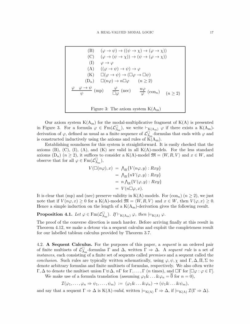
(B) (ϕ→ ψ) → ((ψ → χ) → (ϕ→ χ))
(C) (ϕ→ (ψ → χ)) → (ψ → (ϕ→ χ))
(I) ϕ→ ϕ
(A) ((ϕ→ ψ) → ψ) → ϕ
(K) (ϕ→ ψ) → (ϕ→ ψ)
(Dn) (nϕ) → nϕ (n ≥ 2)
ϕ ϕ→ ψ
ψ(mp)
ϕ
ϕ(nec) nϕ
ϕ (conn) (n ≥ 2)
Figure 3: The axiom system K(Am)
Our axiom system K(Am) for the modal-multiplicative fragment of K(A) is presentedin Figure 3. For a formula ϕ ∈ Fm(L
Am), we write ⊢K(Am) ϕ if there exists a K(Am)-
derivation of ϕ, defined as usual as a finite sequence of LAm
-formulas that ends with ϕ andis constructed inductively using the axioms and rules of K(Am).
Establishing soundness for this system is straightforward. It is easily checked that theaxioms (B), (C), (I), (A), and (K) are valid in all K(A)-models. For the less standardaxioms (Dn) (n ≥ 2), it suffices to consider a K(A)-model M = 〈W,R, V 〉 and x ∈ W , andobserve that for all ϕ ∈ Fm(L
Am),
V ((nϕ), x) =∧
RV (nϕ, y) : Rxy
=∧
RnV (ϕ, y) : Rxy
= n∧
RV (ϕ, y) : Rxy
= V (nϕ, x).
It is clear that (mp) and (nec) preserve validity in K(A)-models. For (conn) (n ≥ 2), we justnote that if V (nϕ, x) ≥ 0 for a K(A)-model M = 〈W,R, V 〉 and x ∈ W , then V (ϕ, x) ≥ 0.Hence a simple induction on the length of a K(Am)-derivation gives the following result.
Proposition 4.1. Let ϕ ∈ Fm(LAm
). If ⊢K(Am) ϕ, then |=K(A) ϕ.
The proof of the converse direction is much harder. Before arriving finally at this result inTheorem 4.12, we make a detour via a sequent calculus and exploit the completeness resultfor our labelled tableau calculus provided by Theorem 3.7.
4.2. A Sequent Calculus. For the purposes of this paper, a sequent is an ordered pairof finite multisets of L
Am-formulas Γ and ∆, written Γ ⇒ ∆. A sequent rule is a set of
instances, each consisting of a finite set of sequents called premises and a sequent called theconclusion. Such rules are typically written schematically, using ϕ,ψ, χ and Γ,∆,Π,Σ todenote arbitrary formulas and finite multisets of formulas, respectively. We also often writeΓ,∆ to denote the multiset union Γ⊎∆, nΓ for Γ, . . . ,Γ (n times), and Γ for [ϕ : ϕ ∈ Γ].
We make use of a formula translation (assuming ϕ1& . . .&ϕn = 0 for n = 0),
I(ϕ1, . . . , ϕn ⇒ ψ1, . . . , ψm) := (ϕ1& . . .&ϕn) → (ψ1& . . .&ψm),
and say that a sequent Γ ⇒ ∆ is K(A)-valid, written |=K(A) Γ ⇒ ∆, if |=K(A) I(Γ ⇒ ∆).
18 D. DIACONESCU, G. METCALFE, AND L. SCHNURIGER
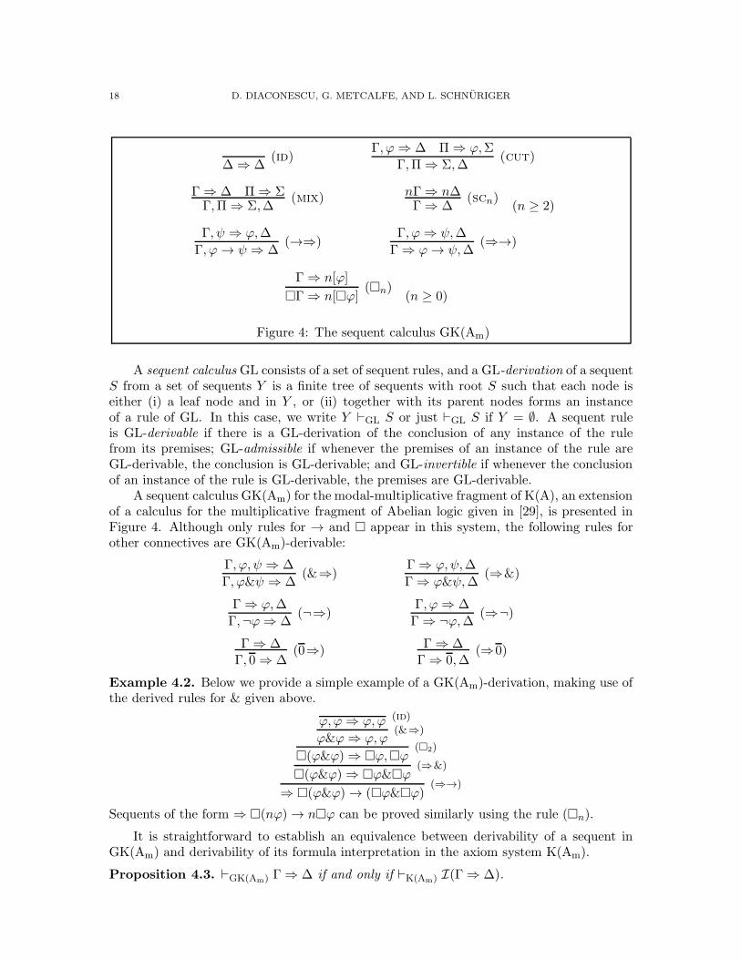
∆ ⇒ ∆(id)
Γ, ϕ⇒ ∆ Π ⇒ ϕ,Σ
Γ,Π ⇒ Σ,∆(cut)
Γ ⇒ ∆ Π ⇒ ΣΓ,Π ⇒ Σ,∆
(mix) nΓ ⇒ n∆Γ ⇒ ∆
(scn) (n ≥ 2)
Γ, ψ ⇒ ϕ,∆
Γ, ϕ→ ψ ⇒ ∆(→⇒)
Γ, ϕ⇒ ψ,∆
Γ ⇒ ϕ→ ψ,∆(⇒→)
Γ ⇒ n[ϕ]
Γ ⇒ n[ϕ](n)
(n ≥ 0)
Figure 4: The sequent calculus GK(Am)
A sequent calculus GL consists of a set of sequent rules, and a GL-derivation of a sequentS from a set of sequents Y is a finite tree of sequents with root S such that each node iseither (i) a leaf node and in Y , or (ii) together with its parent nodes forms an instanceof a rule of GL. In this case, we write Y ⊢GL S or just ⊢GL S if Y = ∅. A sequent ruleis GL-derivable if there is a GL-derivation of the conclusion of any instance of the rulefrom its premises; GL-admissible if whenever the premises of an instance of the rule areGL-derivable, the conclusion is GL-derivable; and GL-invertible if whenever the conclusionof an instance of the rule is GL-derivable, the premises are GL-derivable.
A sequent calculus GK(Am) for the modal-multiplicative fragment of K(A), an extensionof a calculus for the multiplicative fragment of Abelian logic given in [29], is presented inFigure 4. Although only rules for → and appear in this system, the following rules forother connectives are GK(Am)-derivable:
Γ, ϕ, ψ ⇒ ∆
Γ, ϕ&ψ ⇒ ∆(&⇒)
Γ ⇒ ϕ,ψ,∆
Γ ⇒ ϕ&ψ,∆(⇒&)
Γ ⇒ ϕ,∆
Γ,¬ϕ⇒ ∆(¬⇒)
Γ, ϕ⇒ ∆
Γ ⇒ ¬ϕ,∆(⇒¬)
Γ ⇒ ∆Γ, 0 ⇒ ∆
(0⇒)Γ ⇒ ∆
Γ ⇒ 0,∆(⇒0)
Example 4.2. Below we provide a simple example of a GK(Am)-derivation, making use ofthe derived rules for & given above.
ϕ,ϕ⇒ ϕ,ϕ (id)
ϕ&ϕ⇒ ϕ,ϕ(&⇒)
(ϕ&ϕ) ⇒ ϕ,ϕ(2)
(ϕ&ϕ) ⇒ ϕ&ϕ(⇒&)
⇒ (ϕ&ϕ) → (ϕ&ϕ)(⇒→)
Sequents of the form ⇒ (nϕ) → nϕ can be proved similarly using the rule (n).
It is straightforward to establish an equivalence between derivability of a sequent inGK(Am) and derivability of its formula interpretation in the axiom system K(Am).
Proposition 4.3. ⊢GK(Am) Γ ⇒ ∆ if and only if ⊢K(Am) I(Γ ⇒ ∆).

A REAL-VALUED MODAL LOGIC 19
Proof. It suffices for the left-to-right direction to show that for any rule of GK(Am) withpremises S1, . . . , Sm and conclusion S, whenever ⊢K(Am) I(Si) for each i ∈ 1, . . . ,m,also ⊢K(Am) I(S). For example, consider the rule (n) and assume that ⊢K(A) I(Γ ⇒ n[ϕ]).Suppose that Γ = [ψ1, . . . , ψm] and let ψ = ψ1& . . .&ψm. We continue the K(Am)-derivationof I(Γ ⇒ n[ϕ]) = ψ → nϕ to obtain a K(Am)-derivation of ψ → nϕ:
1. ψ → nϕ
2. (ψ → nϕ) (nec)3. (ψ → nϕ) → (ψ → nϕ) (K)4. ψ → nϕ (mp) with 2,35. nϕ→ nϕ (Dn)6. (ψ → nϕ) → ((nϕ→ nϕ) → (ψ → nϕ)) (B)7. (nϕ→ nϕ) → (ψ → nϕ) (mp) with 4,68. ψ → nϕ (mp) with 5,7.
(ψ1& . . .&ψm) → ψ is derivable using (B), (C), (I), and (K), so, using (B) and (mp),we obtain a K(Am)-derivation of I(Γ ⇒ n[ϕ]) = (ψ1& . . .&ψm) → nϕ.
For the right-to-left direction, it is easy to show that every axiom of K(Am) is GK(Am)-derivable; see, e.g., Example 4.2 for GK(Am)-derivations of instances of (Dn). Also, the rulesof K(Am) are GK(Am)-derivable. For example, for (conn), starting with ⇒ nϕ, we apply(cut) with the GK(Am)-derivable sequent nϕ⇒ n[ϕ] to obtain ⇒ n[ϕ] and then, applying(scn), also ⇒ ϕ. Hence, if ⊢K(Am) I(Γ ⇒ ∆), then ⊢GK(Am)⇒ I(Γ ⇒ ∆) and, applying(cut) with the GK(Am)-derivable sequent Γ,I(Γ ⇒ ∆) ⇒ ∆, also ⊢GK(Am) Γ ⇒ ∆.
We now consider a more complicated family of rules, indexed by k ∈ N \0 and n ∈ N,that will be very useful in subsequent cut-elimination and completeness proofs:
Γ0 ⇒ Γ1 ⇒ k[ϕ1] . . . Γn ⇒ k[ϕn]
∆,Γ ⇒ ϕ1, . . . ,ϕn,∆(k,n)
where kΓ = Γ0 ⊎ Γ1 ⊎ . . . ⊎ Γn.
Critically for our later considerations, (k,n) is GK(Am)-derivable for all k ∈ N \0, n ∈ N
(for k = 1, omitting the application of (sck)):
∆ ⇒ ∆(id)
Γ0 ⇒Γ0 ⇒
(0)
Γ1 ⇒ k[ϕ1]
Γ1 ⇒ k[ϕ1](k)
Γn ⇒ k[ϕn]
Γn ⇒ k[ϕn](k)
...
(mix)
(Γ1 ⊎ . . . ⊎ Γn) ⇒ k[ϕ1], . . . , k[ϕn](mix)
(Γ0 ⊎ Γ1 ⊎ . . . ⊎ Γn) ⇒ k[ϕ1], . . . , k[ϕn](mix)
Γ ⇒ ϕ1, . . . ,ϕn(sck)
∆,Γ ⇒ ϕ1, . . . ,ϕn,∆(mix)
We devote the remainder of this subsection to showing that the calculus GK(Am) admitscut-elimination. That is, we provide an algorithm for constructively eliminating applicationsof the rule (cut) from GK(Am)-derivations. Observe first that the “cancellation” rule
Γ, ϕ⇒ ϕ,∆
Γ ⇒ ∆(can)
is both GK(Am)-derivable and can be used, with (mix), to derive (cut):
20 D. DIACONESCU, G. METCALFE, AND L. SCHNURIGER
ϕ⇒ ϕ (id)
ϕ→ ϕ⇒ (→⇒)Γ, ϕ⇒ ϕ,∆
Γ ⇒ ϕ→ ϕ,∆(⇒→)
Γ ⇒ ∆(cut)
Γ, ϕ⇒ ∆ Π ⇒ ϕ,Σ
Γ,Π, ϕ ⇒ ϕ,Σ,∆(mix)
Γ,Π ⇒ Σ,∆(can)
Hence, to prove cut-elimination, it will be enough to show constructively that (can) isadmissible in GK(Am) without (cut).
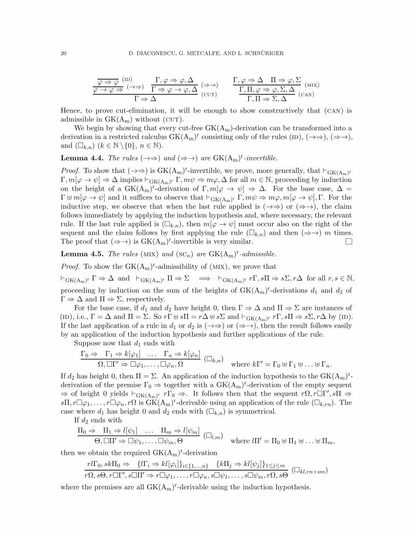
We begin by showing that every cut-free GK(Am)-derivation can be transformed into aderivation in a restricted calculus GK(Am)r consisting only of the rules (id), (→⇒), (⇒→),and (k,n) (k ∈ N \0, n ∈ N).
Lemma 4.4. The rules (→⇒) and (⇒→) are GK(Am)r-invertible.
Proof. To show that (→⇒) is GK(Am)r-invertible, we prove, more generally, that ⊢GK(Am)r
Γ,m[ϕ→ ψ] ⇒ ∆ implies ⊢GK(Am)r Γ,mψ ⇒ mϕ,∆ for all m ∈ N, proceeding by inductionon the height of a GK(Am)r-derivation of Γ,m[ϕ → ψ] ⇒ ∆. For the base case, ∆ =Γ ⊎m[ϕ → ψ] and it suffices to observe that ⊢GK(Am)r Γ,mψ ⇒ mϕ,m[ϕ → ψ],Γ. For theinductive step, we observe that when the last rule applied is (→⇒) or (⇒→), the claimfollows immediately by applying the induction hypothesis and, where necessary, the relevantrule. If the last rule applied is (k,n), then m[ϕ → ψ] must occur also on the right of thesequent and the claim follows by first applying the rule (k,n) and then (⇒→) m times.The proof that (⇒→) is GK(Am)r-invertible is very similar.
Lemma 4.5. The rules (mix) and (scn) are GK(Am)r-admissible.
Proof. To show the GK(Am)r-admissibility of (mix), we prove that
⊢GK(Am)r Γ ⇒ ∆ and ⊢GK(Am)r Π ⇒ Σ =⇒ ⊢GK(Am)r rΓ, sΠ ⇒ sΣ, r∆ for all r, s ∈ N,
proceeding by induction on the sum of the heights of GK(Am)r-derivations d1 and d2 ofΓ ⇒ ∆ and Π ⇒ Σ, respectively.
For the base case, if d1 and d2 have height 0, then Γ ⇒ ∆ and Π ⇒ Σ are instances of(id), i.e., Γ = ∆ and Π = Σ. So rΓ ⊎ sΠ = r∆ ⊎ sΣ and ⊢GK(Am)r rΓ, sΠ ⇒ sΣ, r∆ by (id).If the last application of a rule in d1 or d2 is (→⇒) or (⇒→), then the result follows easilyby an application of the induction hypothesis and further applications of the rule.
Suppose now that d1 ends with
Γ0 ⇒ Γ1 ⇒ k[ϕ1] . . . Γn ⇒ k[ϕn]
Ω,Γ′ ⇒ ϕ1, . . . ,ϕn,Ω(k,n)
where kΓ′ = Γ0 ⊎ Γ1 ⊎ . . . ⊎ Γn.
If d2 has height 0, then Π = Σ. An application of the induction hypothesis to the GK(Am)r-derivation of the premise Γ0 ⇒ together with a GK(Am)r-derivation of the empty sequent⇒ of height 0 yields ⊢GK(Am)r rΓ0 ⇒. It follows then that the sequent rΩ, rΓ′, sΠ ⇒sΠ, rϕ1, . . . , rϕn, rΩ is GK(Am)r-derivable using an application of the rule (k,rn). Thecase where d1 has height 0 and d2 ends with (k,n) is symmetrical.
If d2 ends with
Π0 ⇒ Π1 ⇒ l[ψ1] . . . Πm ⇒ l[ψm]
Θ,Π′ ⇒ ψ1, . . . ,ψm,Θ(l,m)
where lΠ′ = Π0 ⊎ Π1 ⊎ . . . ⊎ Πm,
then we obtain the required GK(Am)r-derivation
rlΓ0, skΠ0 ⇒ lΓi ⇒ kl[ϕi]i∈1,...,n kΠj ⇒ kl[ψj ]1≤j≤m
rΩ, sΘ, rΓ′, sΠ′ ⇒ rϕ1, . . . , rϕn, sψ1, . . . , sψm, rΩ, sΘ(kl,rn+sm)
where the premises are all GK(Am)r-derivable using the induction hypothesis.
A REAL-VALUED MODAL LOGIC 21
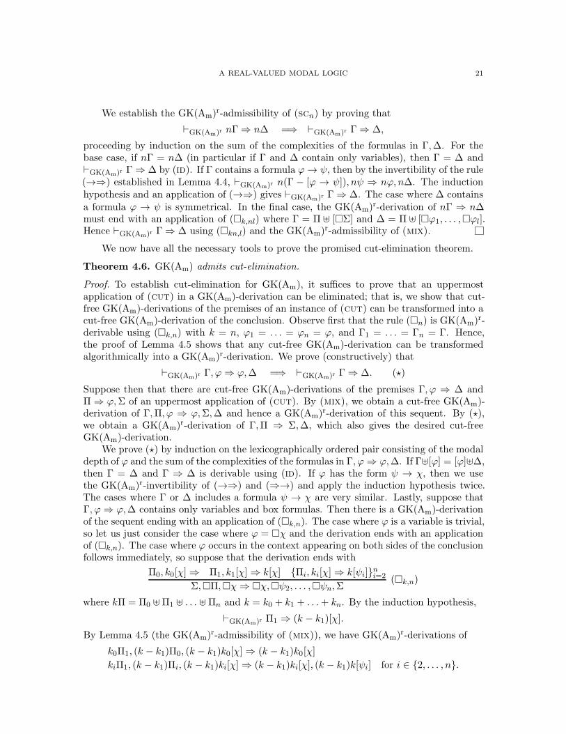
We establish the GK(Am)r-admissibility of (scn) by proving that
⊢GK(Am)r nΓ ⇒ n∆ =⇒ ⊢GK(Am)r Γ ⇒ ∆,
proceeding by induction on the sum of the complexities of the formulas in Γ,∆. For thebase case, if nΓ = n∆ (in particular if Γ and ∆ contain only variables), then Γ = ∆ and⊢GK(Am)r Γ ⇒ ∆ by (id). If Γ contains a formula ϕ→ ψ, then by the invertibility of the rule(→⇒) established in Lemma 4.4, ⊢GK(Am)r n(Γ − [ϕ → ψ]), nψ ⇒ nϕ, n∆. The inductionhypothesis and an application of (→⇒) gives ⊢GK(Am)r Γ ⇒ ∆. The case where ∆ containsa formula ϕ → ψ is symmetrical. In the final case, the GK(Am)r-derivation of nΓ ⇒ n∆must end with an application of (k,nl) where Γ = Π ⊎ [Σ] and ∆ = Π ⊎ [ϕ1, . . . ,ϕl].Hence ⊢GK(Am)r Γ ⇒ ∆ using (kn,l) and the GK(Am)r-admissibility of (mix).
We now have all the necessary tools to prove the promised cut-elimination theorem.
Theorem 4.6. GK(Am) admits cut-elimination.
Proof. To establish cut-elimination for GK(Am), it suffices to prove that an uppermostapplication of (cut) in a GK(Am)-derivation can be eliminated; that is, we show that cut-free GK(Am)-derivations of the premises of an instance of (cut) can be transformed into acut-free GK(Am)-derivation of the conclusion. Observe first that the rule (n) is GK(Am)r-derivable using (k,n) with k = n, ϕ1 = . . . = ϕn = ϕ, and Γ1 = . . . = Γn = Γ. Hence,the proof of Lemma 4.5 shows that any cut-free GK(Am)-derivation can be transformedalgorithmically into a GK(Am)r-derivation. We prove (constructively) that
⊢GK(Am)r Γ, ϕ⇒ ϕ,∆ =⇒ ⊢GK(Am)r Γ ⇒ ∆. (⋆)
Suppose then that there are cut-free GK(Am)-derivations of the premises Γ, ϕ ⇒ ∆ andΠ ⇒ ϕ,Σ of an uppermost application of (cut). By (mix), we obtain a cut-free GK(Am)-derivation of Γ,Π, ϕ ⇒ ϕ,Σ,∆ and hence a GK(Am)r-derivation of this sequent. By (⋆),we obtain a GK(Am)r-derivation of Γ,Π ⇒ Σ,∆, which also gives the desired cut-freeGK(Am)-derivation.
We prove (⋆) by induction on the lexicographically ordered pair consisting of the modaldepth of ϕ and the sum of the complexities of the formulas in Γ, ϕ⇒ ϕ,∆. If Γ⊎[ϕ] = [ϕ]⊎∆,then Γ = ∆ and Γ ⇒ ∆ is derivable using (id). If ϕ has the form ψ → χ, then we usethe GK(Am)r-invertibility of (→⇒) and (⇒→) and apply the induction hypothesis twice.The cases where Γ or ∆ includes a formula ψ → χ are very similar. Lastly, suppose thatΓ, ϕ⇒ ϕ,∆ contains only variables and box formulas. Then there is a GK(Am)-derivationof the sequent ending with an application of (k,n). The case where ϕ is a variable is trivial,so let us just consider the case where ϕ = χ and the derivation ends with an applicationof (k,n). The case where ϕ occurs in the context appearing on both sides of the conclusionfollows immediately, so suppose that the derivation ends with
Π0, k0[χ] ⇒ Π1, k1[χ] ⇒ k[χ] Πi, ki[χ] ⇒ k[ψi]ni=2
Σ,Π,χ⇒ χ,ψ2, . . . ,ψn,Σ(k,n)
where kΠ = Π0 ⊎ Π1 ⊎ . . . ⊎ Πn and k = k0 + k1 + . . .+ kn. By the induction hypothesis,
⊢GK(Am)r Π1 ⇒ (k − k1)[χ].
By Lemma 4.5 (the GK(Am)r-admissibility of (mix)), we have GK(Am)r-derivations of
k0Π1, (k − k1)Π0, (k − k1)k0[χ] ⇒ (k − k1)k0[χ]
kiΠ1, (k − k1)Πi, (k − k1)ki[χ] ⇒ (k − k1)ki[χ], (k − k1)k[ψi] for i ∈ 2, . . . , n.

22 D. DIACONESCU, G. METCALFE, AND L. SCHNURIGER
So, by the induction hypothesis, we have GK(Am)r-derivations of
k0Π1, (k − k1)Π0 ⇒
kiΠ1, (k − k1)Πi ⇒ (k − k1)k[ψi] for i ∈ 2, . . . , n.
Now by an application of ((k−k1)k,n−1), we have a GK(Am)r-derivation ending with
k0Π1, (k − k1)Π0 ⇒ kiΠ1, (k − k1)Πi ⇒ (k − k1)k[ψi]ni=2
Σ,Π ⇒ ψ2, . . . ,ψn,Σ
where (k − k1)kΠ = (k0 + k2 + . . .+ kn)(Π0 ⊎ Π1 ⊎ . . . ⊎ Πn).
4.3. Completeness. In this section we establish the completeness of both the axiom systemK(Am) and the sequent calculus GK(Am) for the modal-multiplicative fragment of K(A).The crucial ingredient of our proof will be the fact that an LK′(A)-tableau for an L
Am-
formula always consists of just one branch, and hence a single inconsistent system of linearinequations can be associated with each valid L
Am-formula.
We begin by proving two lemmas for K(A)-valid sequents of a certain form, recallingthat sequents contain only L
Am-formulas by definition.
Lemma 4.7. Let Γ,Π ⇒ Σ,∆ be a K(A)-valid sequent such that no variable occurs in bothΓ ⊎ ∆ and Π ⊎ Σ. Then Γ ⇒ ∆ and Π ⇒ Σ are both K(A)-valid.
Proof. Suppose contrapositively that 6|=K(A) Γ ⇒ ∆. Then there exists a K(A)-modelM = 〈W,R, V 〉 and x ∈ W such that V (I(Γ ⇒ ∆), x) < 0. Since Γ ⊎ ∆ and Π ⊎ Σ havedisjoint sets of variables, we may assume without loss of generality that V (p, y) = 0 for allp ∈ Var occurring in Π ⊎ Σ and y ∈ W . A simple induction yields also that V (ϕ, y) = 0for all ϕ ∈ Π ⊎ Σ and y ∈ W . But then V (I(Γ,Π ⇒ Σ,∆), x) < 0. So 6|=K(A) Γ,Π ⇒ Σ,∆.The case where 6|=K(A) Π ⇒ Σ follows by symmetry.
Lemma 4.8. Let Γ,Π ⇒ Σ,∆ be a K(A)-valid sequent such that Π and Σ contain onlyvariables. Then Π = Σ and Γ ⇒ ∆ is K(A)-valid.
Proof. Suppose that |=K(A) Γ,Π ⇒ Σ,∆. It suffices to show that Π = Σ, since thenclearly also |=K(A) Γ ⇒ ∆. Suppose for a contradiction that Π 6= Σ. Without loss ofgenerality, some p ∈ Var occurs strictly more times in Π than Σ. Consider a K(A)-modelM = 〈x, ∅, V 〉 with one irreflexive world x satisfying V (p, x) = 1 and V (q, x) = 0 forall q ∈ Var \ p. Then V (I(Γ,Π ⇒ Σ,∆), x) < 0 and so 6|=K(A) Γ,Π ⇒ Σ,∆, acontradiction.
To deal with K(A)-valid sequents in general, we use the fact that for such a sequent,there must exist a corresponding closed complete LK′(A)-tableau with one branch and anassociated inconsistent set of inequations. We use this set of inequations to show that therule (k,m) for suitable k,m can be applied backwards to the sequent to obtain K(A)-validsequents containing formulas of strictly smaller modal depth. To this end, it will be helpfulto extend some of the notions for the labelled tableau calculus LK′(A) to sequents. Wedefine a complete LK′(A)-tableau for a sequent Γ ⇒ ∆ to be a tableau beginning withthe active inequation (Γ)1 > (∆)1 and relation r12, constructed according to steps (2)–(7).Consulting the proof of Theorem 3.7, we obtain the following result.
Corollary 4.9. There exists a closed complete LK′(A)-tableau for a sequent Γ ⇒ ∆ if andonly if Γ ⇒ ∆ is K(A)-valid.
A REAL-VALUED MODAL LOGIC 23
To argue about the inconsistency of a system of inequations associated to a tableau, werecall some basic notions from linear programming. Let S be a system of inequations of theform Ii = (fi(x) > gi(x)) (i ∈ 1, . . . , n) and Jj = (hj(x) ≥ kj(x)) (j ∈ 1, . . . ,m) whereeach fi, gi, hj , kj is a positive linear sum of variables in x. Then S is inconsistent over R ifand only if there exists an inequation given by a linear combination of these inequations
LS =∑n
i=1 λiIi +∑m
j=1 µjJj
where λ1, . . . , λn ∈ N (not all zero) and µ1, . . . , µm ∈ N such that
λ1f1 + . . .+ λnfn + µ1h1 + . . .+ µmhm = λ1g1 + . . .+ λngn + µ1k1 + . . .+ µmkm.
We say that LS is inconsistent and that each inequation fi(x) > gi(x) or hj(x) ≥ kj(x) isused λi or µj times, respectively, in LS .
Given a labelled inequation I = (Γ1)k1 ⊲ (∆1)l1 , let IE = (Γ2)k2 ⊲ (∆2)l2 be the inequa-
tion obtained by applying the rules for → in LK′(A) to I exhaustively. By further replacingeach boxed formula ϕ with ⌈ϕ⌉, we obtain the reduced form IR of I, saying that I is inreduced form if I = IR. We now have all the required tools to prove our main lemma.
Lemma 4.10. Let Γ ⇒ ψ1, . . . ,ψm be a K(A)-valid sequent. Then there exist k ∈N \0 and multisets of L
Am-formulas Γ0,Γ1, . . . ,Γm such that
(i) kΓ = Γ0 ⊎ Γ1 ⊎ . . . ⊎ Γm
(ii) Γ0 ⇒ and Γi ⇒ k[ψi] for i ∈ 1, . . . ,m are all K(A)-valid.
Proof. Let Γ = [ϕ1, . . . , ϕn]. By assumption, |=K(A) ϕ1, . . . ,ϕn ⇒ ψ1, . . . ,ψm, and,
by Corollary 4.9, we obtain a complete closed tableau T in LK′(A) that begins with
(ϕ1)1, . . . , (ϕn)1 > (ψ1)1, . . . , (ψm)1 and r12.
This tableau will contain the inequation
I = (⌈ϕ1⌉)1, . . . , (⌈ϕn⌉)
1 > (⌈ψ1⌉)1, . . . , (⌈ψm⌉)1
and for new labels y1, . . . , ym ∈ N, the inequations
I1 = (⌈ψ1⌉)1 ≥ (ψ1)y1 . . . Im = (⌈ψm⌉)1 ≥ (ψm)ym .
Let us fix y0 = 2. Then T contains for each i ∈ 1, . . . , n and j ∈ 0, . . . ,m, an inequation
Ii,j = (ϕi)yj ≥ (⌈ϕi⌉)
1.
Consider now the set of inequations associated to T
S = I ∪ IRj : 1 ≤ j ≤ m ∪ IRij : 1 ≤ i ≤ n, 0 ≤ j ≤ m ∪ S′,
noting that the inequations in S′ are obtained by applying rules of LK′(A) to inequationsin IEj : 1 ≤ j ≤ m ∪ IEij : 1 ≤ i ≤ n, 0 ≤ j ≤ m. Since T is closed, S is inconsistentover R. Hence there is an inconsistent linear combination LS of the inequations in S. Thefollowing observations can be confirmed by simple inductions on the height of T :
(i) The (reduced form) inequation I is the only strict inequation occurring in S, andhence must be used k times in LS for some k ∈ N \0.
(ii) For each j ∈ 1, . . . ,m, (⌈ψj⌉)1 occurs in S only in I and in the reduced form IRj
of Ij ; hence, by (i), IRj must also be used k times in LS.

24 D. DIACONESCU, G. METCALFE, AND L. SCHNURIGER
(iii) For each i ∈ 1, . . . , n, (⌈ϕi⌉)1 occurs in S only in I and in the reduced forms IRi,j
of Ii,j for j ∈ 0, . . . ,m; hence, given that IRi,j is used in the linear combination λi,jtimes, we obtain λi,0 + λi,1 + . . .+ λi,m = k; in particular, not all λi,j are zero.
The inconsistent linear combination of the inequations in S is therefore
LS = kI +∑m
j=1 kIRj +
∑ni=1
∑mj=0 λi,jI
Ri,j + LS′ .
We define multisets of formulas
Γj = λ1,j[ϕ1], . . . , λn,j [ϕn] for j ∈ 0, . . . ,m
∆ = k[⌈ϕ1⌉], . . . , k[⌈ϕn⌉], k[⌈ψ1⌉], . . . , k[⌈ψm⌉].
Note that, as required, kΓ = Γ0 ⊎ Γ1 ⊎ . . . ⊎ Γm. Consider now the inequation
J = kI +∑m
j=1 kIj +∑n
i=1
∑mj=0 λi,jIi,j
= (Γ0)y0 , (Γ1)y1 , . . . , (Γm)ym , (∆)1 > (∆)1, k[(ψ1)y1 ], . . . , k[(ψm)ym ].
Then LS = JR + LS′ and the set of inequations S∗ = JR ∪ S′ is inconsistent over R.Recall that each (reduced form) inequation in S′ is obtained by applying rules of LK′(A)
to the inequations IEj : 1 ≤ j ≤ m ∪ IEij : 1 ≤ i ≤ n, 0 ≤ j ≤ m. But following the
procedure for building a complete LK′(A)-tableau, the inequations in S′ are obtained byfirst applying the rules ( ⊲′) and (⊲′). Hence these inequations in S′ and JR are alsoobtained by first applying the rules ( ⊲′) and (⊲′) to JE and then continuing as before.
Now for each j ∈ 0, . . . ,m, let Varj ⊆ Var be a countably infinite set such thatVar0 ∩ Var1 ∩ . . . ∩ Varm = ∅, and let hj : Var → Varj be a bijective map that extends inthe obvious way to all formulas and multisets of formulas. Consider the inequation
J ′ = (h0(Γ0))1, (h1(Γ1))1, . . . , (hm(Γm))1, (∆)1 > (∆)1, k[(h1(ψ1))1], . . . , k[(hm(ψm))1].
An easy induction on the height of a tableau shows that applying the rules of LK′(A) to J ′
and relation r12 also produces a set of inequations that is inconsistent over R. But then byCorollary 4.9,
|=K(A) h0(Γ0), h1(Γ1), . . . , hm(Γm),∆ ⇒ ∆, k[h1(ψ1)], . . . , k[hm(ψm)].
Applying Lemma 4.7 repeatedly, we obtain
|=K(A) h0(Γ0) ⇒ and |=K(A) hi(Γi) ⇒ k[hi(ψi)] for i ∈ 1, . . . ,m,
and hence, renaming variables,
|=K(A) Γ0 ⇒ and |=K(A) Γi ⇒ k[ψi] for i ∈ 1, . . . ,m
as required.
Proposition 4.11. Let Γ ⇒ ∆ be a K(A)-valid sequent. Then ⊢GK(Am) Γ ⇒ ∆.
Proof. We prove the claim by induction on the lexicographically ordered pair consisting ofthe modal depth of I(Γ ⇒ ∆) and the sum of the complexities of the formulas in Γ ⊎ ∆.
For the base case, suppose that |=K(A) Γ ⇒ ∆ and that both Γ and ∆ contain onlyvariables. Then, by Lemma 4.8, we obtain Γ = ∆. Hence, by (id), we get ⊢GK(Am) Γ ⇒ ∆.
For the inductive step, suppose first that |=K(A) Γ, ϕ → ψ ⇒ ∆. Then also |=K(A)
Γ, ψ ⇒ ϕ,∆. So by the induction hypothesis, ⊢GK(Am) Γ, ψ ⇒ ϕ,∆. Hence, by (→⇒), weget ⊢GK(Am) Γ, ϕ→ ψ ⇒ ∆. The case where ϕ→ ψ occurs on the right is very similar.
Now suppose that |=K(A) Γ,Π ⇒ Σ,ψ1, . . . ,ψm where Π and Σ contain onlyvariables. By Lemma 4.8, we obtain Π = Σ and |=K(A) Γ ⇒ ψ1, . . . ,ψm. By (id),

A REAL-VALUED MODAL LOGIC 25
we get ⊢GK(Am) Π ⇒ Σ. Moreover, by Lemma 4.10, there exist k ∈ N \0 and multisets of
LAm
-formulas Γ0,Γ1, . . . ,Γm such that
(i) kΓ = Γ0 ⊎ Γ1 ⊎ . . . ⊎ Γm
(ii) |=K(A) Γ0 ⇒ and |=K(A) Γi ⇒ k[ψi] for i ∈ 1, . . . ,m.
But then by the induction hypothesis also
(iii) ⊢GK(Am) Γ0 ⇒ and ⊢GK(Am) Γi ⇒ k[ψi] for i ∈ 1, . . . ,m.
Hence, using the GK(Am)-derivable rule (k,m), we obtain ⊢GK(Am) Γ ⇒ ψ1, . . . ,ψm.Finally, using (mix), we obtain ⊢GK(Am) Γ,Π ⇒ Σ,ψ1, . . . ,ψm as required.
Our main theorem now follows as a direct combination of Propositions 4.1, 4.3, and 4.11.
Theorem 4.12. The following are equivalent for any ϕ ∈ Fm(LAm
):
(1) |=K(A) ϕ.(2) ⊢K(Am) ϕ.(3) ⊢GK(Am)⇒ϕ.
Let us remark finally that, since any LK′(A)-tableau for an LAm
-formula has just onebranch, we obtain (consulting the proof of Theorem 3.8) a smaller upper bound for thecomplexity of checking K(A)-validity in this fragment.
Theorem 4.13. The problem of checking if ϕ ∈ Fm(LAm
) is K(A)-valid is in EXPTIME.
5. Concluding Remarks
This paper takes a significant step towards a proof-theoretic account of continuous modallogics: many-valued modal logics with connectives interpreted locally by continuous func-tions over sets of real numbers. We have introduced here a minimal modal extension K(A) ofAbelian logic (see [31, 9, 29]), where propositional connectives are interpreted using lattice-ordered group operations over the real numbers, and shown that the modal Lukasiewiczlogic K(Ł) studied in [21] is a fragment of this logic with an additional constant. We haveprovided a labelled tableau calculus for K(A) and established a coNEXPTIME upperbound for checking validity. More significantly, for the modal-multiplicative fragment ofK(A), we have obtained both a sequent calculus that admits cut-elimination and an ax-iomatization without infinitary rules. Notably, this latter result was established using thecompleteness of the labelled tableau calculus to derive a corresponding proof in the sequentcalculus. The more standard algebraic approach to proving completeness of many-valuedmodal logics, employed, e.g., for finite-valued Lukasiewicz modal logics in [21], proceeds byconstructing a canonical model as the set of maximal filters of the Lindenbaum-Tarski al-gebra of the logic. For finite-valued Lukasiewicz modal logics, completeness is proved usingthe fact that the appropriate reduct of this algebra is semi-simple, which is not applicablein the infinite-valued case or for the modal-multiplicative fragment of K(A).
Clearly, there are many open questions still to be addressed. The most pressing issueis to find an axiomatization and algebraic semantics for the full logic K(A). We conjecturethat such an axiomatization can be obtained by extending the axiom system HA for Abelianlogic with the axiom schema (K), (Dn) (n ≥ 2) and rules (mp), (nec) from Figure 3, and theaxiom schema (ϕ∧ψ) → (ϕ∧ψ). It can be shown using methods of abstract algebraiclogic that this axiom system is sound and complete with respect to a corresponding variety
26 D. DIACONESCU, G. METCALFE, AND L. SCHNURIGER
of algebras with a lattice-ordered abelian group reduct; the difficulty of course is to provethat the axiomatization is complete with respect to the frame semantics of K(A), perhapsby extending the proof for the modal-multiplicative fragment (using the labelled tableaucalculus and a Gentzen-style calculus), or via an alternative representation of the algebras.Such a proof would provide the basis for an axiomatization and algebraic semantics for K(Ł),and, more generally, a starting point for a Jonsson-Tarski-style account of the relationshipbetween relational and algebraic semantics for these logics. Note that we can already developsuch a relationship for the modal-multiplicative fragment axiomatized in this paper, but thealgebras corresponding to the axiom system K(Am) will not form a variety.
We have focussed in this work only on the minimal modal extension of Abelian logic.However, adapting the Kripke semantics and labelled tableau calculi to other (e.g., reflexive,symmetric, transitive) classes of frames is a straightforward exercise. More challenging isthe problem of adapting the completeness proofs for the modal-multiplicative fragment tosuitably extended axiom systems and sequent calculi. For the reflexive case, completenessproofs, similar to those given here, can be obtained for the extension of the axiom systemK(Am) with the axiom schema ϕ→ ϕ and the sequent calculus GK(Am) with the rule
Γ, ϕ⇒ ∆
Γ,ϕ⇒ ∆
However, a general approach for tackling different classes of frames is still lacking.Finally, it remains to determine whether the upper bounds given here for the complexity
of checking K(A)-validity are optimal. Let us just note that it makes sense to first investigatethe EXPTIME upper bound for the modal-multiplicative fragment, before considering thecoNEXPTIME upper bound for the full logic K(A) and indeed also K(Ł).
References
[1] F. Baader, S. Borgwardt, and R. Penaloza. Decidability and complexity of fuzzy description logics. KI,31(1):85–90, 2017.
[2] M. Baaz and G. Metcalfe. Herbrand’s theorem, skolemization and proof systems for first-order Lukasiewicz logic. Journal of Logic and Computation, 20(1):35–54, 2008.
[3] S. Baratella. Continuous propositional modal logic. Submitted (available athttp://www.science.unitn.it/~baratell/CPropML.pdf).
[4] F. Bou, M. Cerami, and F. Esteva. Finite-valued Lukasiewicz modal logic is PSPACE-complete. InProceedings of IJCAI 2011, pages 774–779, 2011.
[5] F. Bou, F. Esteva, L. Godo, and R. Rodrıguez. On the minimum many-valued logic over a finiteresiduated lattice. Journal of Logic and Computation, 21(5):739–790, 2011.
[6] X. Caicedo, G. Metcalfe, R. Rodrıguez, and J. Rogger. Decidability in order-based modal logics. Journalof Computer System Sciences, 88:53–74, 2017.
[7] X. Caicedo and R. Rodrıguez. Standard Godel modal logics. Studia Logica, 94(2):189–214, 2010.[8] X. Caicedo and R. Rodrıguez. Bi-modal Godel logic over [0,1]-valued Kripke frames. Journal of Logic
and Computation, 25(1):37–55, 2015.[9] E. Casari. Comparative logics and abelian ℓ-groups. In C. Bonotto, R. Ferro, S. Valentini, and A. Za-
nardo, editors, Logic Colloquium ’88, pages 161–190. Elsevier, 1989.[10] N. Dershowitz and Z. Manna. Proving termination with multiset orderings. Communications of the
Association for Computing Machinery, 22:465–476, 1979.[11] D. Diaconescu and G. Georgescu. Tense operators on MV-algebras and Lukasiewicz-Moisil algebras.
Fundamenta Informaticae, 81(4):379–408, 2007.[12] D. Diaconescu, G. Metcalfe, and L. Schnuriger. Axiomatizing a real-valued modal logic. In Proceedings
of AiML 2016, pages 236–251, 2016.[13] M. C. Fitting. Many-valued modal logics. Fundamenta Informaticae, 15(3–4):235–254, 1991.

A REAL-VALUED MODAL LOGIC 27
[14] M. C. Fitting. Many-valued modal logics II. Fundamenta Informaticae, 17:55–73, 1992.[15] L. Godo, P. Hajek, and F. Esteva. A fuzzy modal logic for belief functions. Fundamenta Informaticae,
57(2–4):127–146, 2003.[16] L. Godo and R. Rodrıguez. A fuzzy modal logic for similarity reasoning. In Fuzzy Logic and Soft
Computing, pages 33–48. Kluwer, 1999.[17] P. Hajek. Metamathematics of Fuzzy Logic. Kluwer, Dordrecht, 1998.[18] P. Hajek. Making fuzzy description logic more general. Fuzzy Sets and Systems, 154(1):1–15, 2005.[19] P. Hajek, D. Harmancova, F. Esteva, P. Garcia, and L. Godo. On modal logics for qualitative possibility
in a fuzzy setting. In Proceedings of UAI 1994, pages 278–285, 1994.[20] P. Hajek, D. Harmancova, and R. Verbrugge. A qualitative fuzzy possibilistic logic. International Jour-
nal of Approximate Reasoning, 12:1–19, 1995.[21] G. Hansoul and B. Teheux. Extending Lukasiewicz logics with a modality: Algebraic approach to
relational semantics. Studia Logica, 101(3):505–545, 2013.[22] L. G. Khachiyan. A polynomial algorithm in linear programming. Soviet Mathematics Doklady, 20:191–
194, 1979.[23] A. Kulacka, D. Pattinson, and L. Schroder. Syntactic labelled tableaux for Lukasiewicz fuzzy ALC. In
Proceedings of IJCAI 2013, pages 962–968, 2013.[24] C. Kupke and D. Pattinson. On modal logics of linear inequalities. In Proceedings of AiML 2010, pages
235–255. King’s College Publications, 2010.[25] M. Marti and G. Metcalfe. Hennessy-Milner properties for many-valued modal logics. In Proceedings of
AiML 2014, pages 407–420. King’s College Publications, 2014.[26] M. Marti and G. Metcalfe. Expressivity of chain-based modal logics. Archive for Mathematical Logic.
To appear.[27] M. Mio and A. Simpson. Lukasiewicz mu-calculus. In Proceedings Workshop on Fixed Points in Com-
puter Science, volume 126 of EPCTS, pages 87–104. Open Publishing Association, 2013.[28] G. Metcalfe and N. Olivetti. Towards a proof theory of Godel modal logics. Logical Methods in Computer
Science, 7(2):1–27, 2011.[29] G. Metcalfe, N. Olivetti, and D. Gabbay. Sequent and hypersequent calculi for abelian and Lukasiewicz
logics. ACM Transactions on Computational Logic, 6(3):578–613, 2005.[30] G. Metcalfe, N. Olivetti, and D. Gabbay. Proof Theory for Fuzzy Logics, volume 36 of Applied Logic.
Springer, 2008.[31] R. K. Meyer and J. K. Slaney. Abelian logic from A to Z. In Paraconsistent Logic: Essays on the
Inconsistent, pages 245–288. Philosophia Verlag, 1989.[32] G. Priest. Many-valued modal logics: a simple approach. Review of Symbolic Logic, 1:190–203, 2008.[33] S. Schockaert, M. De Cock, and E. Kerre. Spatial reasoning in a fuzzy region connection calculus.
Artificial Intelligence, 173(2):258–298, 2009.[34] U. Straccia. Reasoning within fuzzy description logics. Journal of Artificial Intelligence Research, 14:137–
166, 2001.
This work is licensed under the Creative Commons Attribution-NoDerivs License. To view acopy of this license, visit https://creativecommons.org/licenses/by-nd/4.0/ or send aletter to Creative Commons, 171 Second St, Suite 300, San Francisco, CA 94105, USA, orEisenacher Strasse 2, 10777 Berlin, Germany