A reduced model for medial entorhinal cortex

stellate cell: subthreshold oscillations, spiking

and synchronization

Horacio G. Rotstein 1, Tim Oppermann 2,John A. White 3, Nancy Kopell1

1 Department of Mathematics and Center for Biodynamics,

Boston University, Boston, MA, 02215, USA.2 Institute for Theoretical Biology,

Humboldt University Berlin, 10115 Berlin, Germany.3 Department of Biomedical Engineering and Center for Biodynamics,

Boston University, Boston, MA, 02215, USA.

February 16, 2005

Abstract

Entorhinal cortex layer II stellate cells display subthreshold oscil-lations (STOs). We study a single compartment biophysical model ofsuch cells which qualitatively reproduces these STOs. We argue thatin the interspike interval (ISI) the seven-dimensional model can bereduced to a three-dimensional system of equations with well differen-tiated times scales. Using dynamical systems arguments we providea mechanism for generations of STOS. This mechanism is based onthe “canard structure”, in which relevant trajectories stay close torepelling manifolds for a significant interval of time. We also showthat the transition from subthreshold oscillatory activity to spikingis controlled in the ISI by the same structure. The same mechanismis invoked to explain why noise increases the robustness of the STO

2

regime. Taking advantage of the reduction of the dimensionality ofthe full stellate cell system, we propose a generalized integrate-and-fire (GIF) model in which the ISI reduced system is supplementedwith a threshold for spiking and a reset voltage. We show that thesynchronization properties in networks made up of the GIF cells aresimilar to those of networks using the full stellate cell models.

Key words: theta rhythm; reduction of dimensions; Hopf bifur-

cation; canard phenomenon; generalized integrate-and-fire models.

1 Introduction

The flow of information from the neocortex to the hippocampus is orches-trated by the superficial cell layers (II and III) of the enthorinal cortex (EC).The large stellate cells (SCs) of Cajal constitute the most abundant principalcell type in layer II of the medial EC (MEC) and these neurons give rise tothe perforant path, the main afferent fiber system to the hippocampus. In

vivo electrophysiological investigations have shown that the MEC generatestheta rhythm and that the firing of MEC layer II neurons is highly phaselocked to theta field events. Many lines of evidence indicate that the thetarhythm is implicated in learning and memory processes, one of the main func-tions of the medial temporal lobe of which the EC is a crucial component.Importantly, in vitro electrophysiological studies have also established thatthe SCs develop low-amplitude (1-4 mV) rhythmic subthreshold membranepotential oscillations (STOs) at theta frequencies; when the membrane po-tential is set positive to threshold (about -50 mV), SCs fire action potentialsat the peak of the STO but not necessarily at every STO’s cycle (Dicksonet al. 2000b). The coexistence of spiking and subthreshold (mixed-mode)oscillatory activity is a distinctive property of SCs in vitro and the firing ofMEC layer II neurons has also been shown to skip theta cycles in vivo.

The persistent sodium (INap) and h-(Ih) currents have been implicatedin the pacemaking of single-cell rhythmicity at theta frequencies (Dicksonet al. 2000a,b; Magistretti and Alonso 1999; Magistretti and Ragsdale 1999;Alonso and Llinas 1989; Alonso and Klink 1993; Klink and Alonso 1993,1997; Fransen et al. 2004; Gillies et al. 2002; Rotstein et al. 2004) (see alsoreferences therein). The former constitutes a depolarization-activated fastinward current that provides the main drive for the depolarizing phase of theSTOs. The latter, which is a hyperpolarization-activated non-inactivating

3

current with slow kinetics for both activation and deactivation, provides adelayed feedback effect that promotes resonance. (Note that the deactivationof an inward current is equivalent to the activation of an outward current).Theoretical studies, based on simulations of biophysical models, have shownthat the interplay between Ih (with a fast and slow components) and INap maybe sufficient to account for the generation of membrane potential oscillationsin layer II SCs (Dickson et al. 2000a,b; Fransen et al. 1998, 1999; White et al.1995, 1998). However, the dynamic mechanism governing this interaction hasnot yet been explored.

The goal of this paper is to explain the dynamic mechanism governingthe generation of subthreshold oscillations (STO), spikes and mixed-modeoscillatory (MMO) activity in a model of layer II SCs of the MEC which wasintroduced by Acker et al. (2003) to study the synchronization propertiesof SCs. We describe that model in Section 2. It incorporates a INap and atwo-componentIh (fast and slow) in addition to the standard sodium(INa),potassium (IK) and leak (IL) Hodgkin-Huxley (HH) currents.

We argue that, during the largest part of the interspike interval (ISI)regime, INa and IK are inactive, leaving IL, INap, Ih (with its slow and fastcomponents Ihf

and Ihs) as the only active currents. In addition, the INap

gating variable p evolves on a much faster time scale than the rest of theremaining variables, so p is slaved to the voltage. Thus, the essential aspectsof the dynamics of the SC during the ISI can be captured by a reduced three-dimensional system of differential equations, which describes the evolutionof the voltage and the two Ih fast (rf) and slow (rs) gating variables.

At the heart of the mechanism of generation of STOs is a phenomenonassociated with the geometry of invariant manifolds when there are multipletimes scales. When an invariant manifold is unstable, in general trajectoriesstarting near it quickly move away from it. However, if the invariant mani-fold is associated with slower motion, there are circumstances in which thetrajectories starting adequately nearby can stay near the invariant manifoldfor a significant time. This phenomenon is known as a “canard structure”and is associated with a sudden increase in amplitude of the small oscillationsto a large amplitude relaxation oscillation, for example, as some parameter ischanged (Eckhaus 1983; Krupa and Szmolyan 2001; Dumortier and Roussarie1996; Wechselberger 2004).

In this paper, we will not be concerned with large amplitude relaxationoscillation in the ISI regime, but with small amplitude oscillations, corre-sponding to STOs, that follow unstable invariant manifolds for a significant

4

part of the trajectory. The oscillations need not be limit cycles: they mayspiral down to a fixed point, or spiral away from a fixed point. The paperconcerns both these STOs and spikes, which belong to different trajectory“regimes”, in which different ionic currents are important and reduced equa-tions describing the STOs are no longer valid. In our study of the STO’s wewill use an initial condition that approximates the position of the trajectoryafter a spike, which is the relevant initial condition for the start of one or aseries of STO’s.

The canard structure we have in mind is created by the 2D system ofvoltage and fast Ih gating variable. The slow component of Ih controls theSTOs and governs the transition from the STOs to the spiking regimes. Thespike provides a resetting mechanism that brings the system back to the ISIregime (where STOs occur).

One important and useful consequence of our results is that, if one isnot interested in the spike details, the dynamics of the SC can be approxi-mately described by the reduced three-dimensional system mentioned above,supplemented with a threshold for spiking and a reset voltage. We use thisgeneralized integrate-and-fire (GIF) SC model to check the synchronizationproperties of networks of SCs (Acker et al. 2003; Jalics et al. 2004) and toexplain the effects of noise in enhancing the robustness of STOs (White et al.1998).

2 Methods

The single compartment biophysical model we study here was introducedby Acker et al. (2003) and is based on measurements from layer II SCsof the medial entorhinal cortex (MEC) (White et al. 1995, 1998; Dicksonet al. 2000b; Fransen et al. 2004). It has a persistent sodium (INap) and atwo-component (fast and slow) hyperpolarization-activated (Ih) currents inaddition to the standard Hodgkin-Huxley sodium (INa), potassium (IK) andleak (IL) currents. The current-balance equation is

CdV

dt= Iapp − INa − IK − IL − Ih − INap (1)

where V is the membrane potential (mV ), C is the membrane capacitance(µF/cm2), Iapp is the applied bias (DC) current (µA/cm2),INa = GNa m3 h (V − ENa), IK = GK n4 (V − Ek), IL = GL ( V − EL ),

5

INap = Gp p ( V − ENa ), Ih = Gh ( 0.65 rf + 0.35 rs ) ( V − Eh ). GX and EX

(X = Na, K, L, p, h) are the maximal conductances (mS/cm2) and reversalpotentials (mV ) respectively. The units of time are msec. All the gatingvariables x (x = m, h, n, p, rf , rs) obey a first order differential equation ofthe following form:

dx

dt=

x∞(V ) − x

τx(V ), (2)

where

x∞(V ) =αx(V )

αx(V ) + βx(V )and τx(V ) =

1

αx(V ) + βx(V ). (3)

The definitions of αx and βx for x = m, h, n, p, rf , rs are given in theappendix and the corresponding graphs are shown in Fig. 1. The valuesof the parameters used by Acker et al. (2003) are ENa = 55, EK = −90,EL = −65, Eh = −20, GNa = 52, GK = 11, GL = 0.5, Gp = 0.5, Gh = 1.5and C = 1.

Simulations were performed using the modified Euler method and a Runge-Kutta method of order IV (Burden and Faires 1980).

3 Results

3.1 Full model: Coexistence of subthreshold oscilla-

tions and spikes

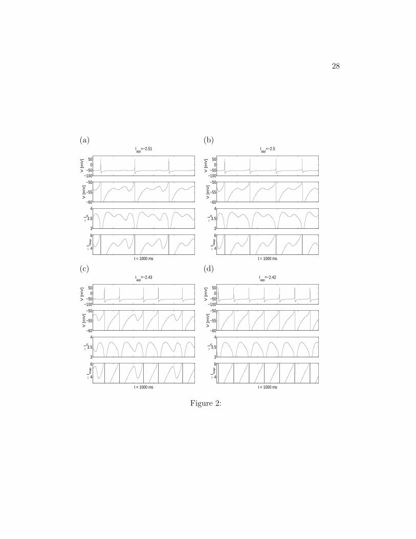
In Fig. 2 we present simulation results for the full SC model for variousvalues of Iapp. The voltage traces are shown in the two top panels (note thatthe second panel is a blow-up of the top panel); the Ih and INap traces aregiven in the two bottom panels. As the value of Iapp increases, the spikingfrequency also increases, while the number of STOs per ISI decreases andfinally vanishes as shown in Fig. 2-d. In all simulations we have done wefound that, for relevant initial conditions, voltage traces either display STOsand spikes, or decay to a fixed point in an oscillatory way. In most cases,STOs increase their amplitude as the SC trajectory approaches spiking.

Our results demonstrating the coexistence of STOs and spikes are consis-tent with experimental findings (Dickson et al. 2000b). However, the STOs

6

predicted using the deterministic full SC model are less robust than exper-imentally found; i.e., the ratio STO/spikes is larger in experiments than insimulations. In Section 3.4 we explain how noise is able to correct for this.

Note that, as experimentally found (Dickson et al. 2000a), INap is ata minimum at the trough of a STO, and Ih reaches its maximum at thebeginning of the depolarizing phase. As depolarization proceeds, INap rapidlyincreases, boosting the depolarization initiated by Ih, which in itself causesthe voltage trajectory to reverse to repolarization. Just after the peak of theoscillation, Ih reaches its minimum

3.2 A reduced SC model valid during the ISI

Here we argue that, during the ISI, INa and IK are almost inactive, leavingINap, Ih and IL as the main active currents. We also show that p ∼ p∞(V ), sothe dynamics of the SC can be approximated by a three-dimensional systemdescribing V , rf and rs. A more precise mathematical analysis of this willbe given in a related work (Rotstein et al. 2005).

3.2.1 Reduced equations

Looking at the second panels in Fig. 2 we see that during most of the ISI thevoltage is bounded between −60 mV and −50 mV . In Figs. 1-e to -f, we seethat for this interval of values of the voltage, τp, τm and τn are much smallerthan τrf

, which we take as a reference time scale. In addition, from Fig.1-d, m∞ ∼ 0 and n4

∞∼ 0. Then m ∼ 0, INa ∼ 0, IK ∼ 0 and p ∼ p∞(v).

Thus, we get the following sytem of equations to approximately describe thedynamics of the SC model during the ISI:

CdV

dt= Iapp − Gp p∞(V ) (V − ENa) − IL − Ih (4)

drf

dt=

rf,∞(V ) − rf

τrf(V )

, (5)

drs

dt=

rs,∞(V ) − rf

τrs(V )

. (6)

As in Eq. (1), Ih = Gh ( 0.65 rf + 0.35 rs ) ( V −Eh ) and IL = GL ( V −EL ).For future use we call Ihf

= Gh 0.65 rf( V −Eh ) and Ihs= Gh 0.35 rs( V −Eh ).

Our simulations with the full SC model (1)-(3) show (data not presented here)

7

that INa < Ihsduring the ISI where STOs occur. In fact, one could describe

this ISI as the interval of time for which INa and IK are inactive in the sensethat they are much lower than the ISI Ih, INap and IL currents.

The voltage bounds during the ISI change with different values of Iapp

and Gh. However, the reduction of dimensions argument used before remainsvalid over a large range of these parameters.

3.2.2 Reset of Ih

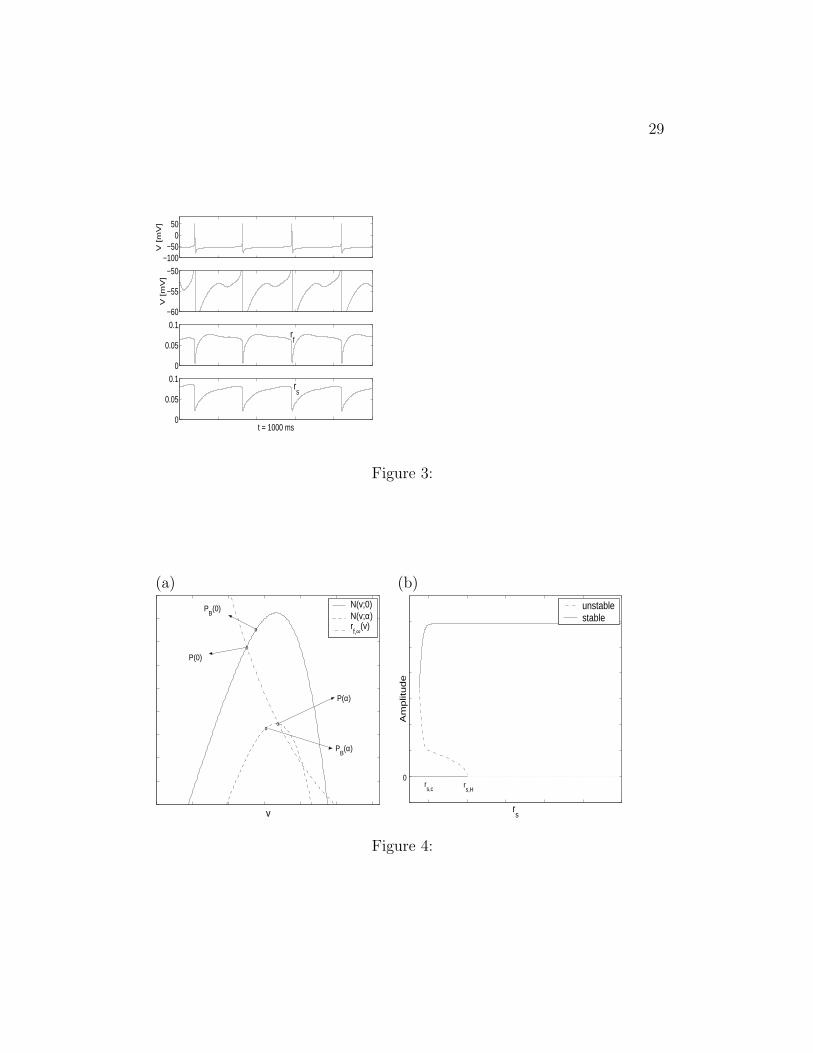
The behavior of v, rf and rs are illustrated in Fig. 3. (The second panelis a blow-up of the first.) During a spike, v increases above zero to a value∼ 50 mV . For these values of v, rf,∞(v) ∼ 0 and rs,∞(v) ∼ 0 (see Fig. 1-a).In addition, for these high values of v, both τrf

(v) and τrs(v) are very small

(see Fig. 1-b and -c), and then both rf and rs quickly decrease to valuesclose to rf ∼ rs ∼ 0. In our approximation we take rf = rs = 0 as initialconditions for the h-current gating variables in the ISI regime (after a spikehas occurred).

3.2.3 A stellate cell generalized integrate and fire model

The fact that INa and IK are inactive during the ISI suggests that if oneis not interested in the spike details but only in the generation of a spike,the dynamics of the SC can be approximately described by a generalizedintegrate-and-fire (GIF) model consisting of eqs. (4)-(6) supplemented witha threshold for spike generation, vth, and a reset value of the membranevoltage, vrst. Appropriate values of vth should reflect the fact that whencrossing threshold, trajectories move towards the spiking regime. In oursimulations we use

vth = −10 mV and vrst = −80 mV. (7)

As will be clear later, more negative values of vth may be good as well.In the full SC model there is a brief intermediate regime in between the

spiking regime and the STO regime studied here (ISI). This regime corre-sponds to the recovery of the voltage after a spike. It is different from theISI regime studied here in that IK is an active current and its gating variablen evolves on a time scale faster than both rf and rs; i.e.. n is a dynamicvariables interacting with v. We disregard this regime in our generalizedintegrate and fire (GIF) formulation.

8

Two- and three-dimensional GIF models have already been proposed inthe literature (Izhikevich 2001; Richardson et al. 2003). In the GIF modelsused by Richardson et al. (2003) to study resonance effects, there is either atwo-component Ih or a INap and IKs (slow K+ current). To our knowledgeno GIF model has been proposed having both Ih and INap. Our GIF modeldescribes the ISI with asymptotic accuracy and is a good approximation ofthe full SC model (1)-(3).

In the following sections we study the dynamics of the SC using thereduced description studied here.

3.3 Dynamics of the reduced SC model

In this Section we study the mechanism of generation of STOs in the SCmodel. These STOs are generated from the dynamics of eqs. (4)-(6).

3.3.1 Canard structures and a study of the reduced model with

rs fixed

The classic canard phenomenon is a sudden explosion of the small amplitudelimit cycle created in a Hopf bifurcation (HB). This small amplitude limitcycle can be stable or unstable according to whether the HB point is super-critical or subcritical respectively. Here, we are concerned with the structurenear an unstable limit cycle, and not the canard explosion itself. In mostof this section, we discuss in as much generality as possible the structurethat we use in analyzing our model. For easy applicability to (4-6), we usenotation tailored to the model. For a more thorough introduction, we referthe reader to Eckhaus (1983); Krupa and Szmolyan (2001); Dumortier andRoussarie (1996).

The general equations have the form

{

dv/dt = F (v, rf ; rs),drf/dt = ε G(v, rf),

(8)

where 0 < ε � 1 and rs is a fixed parameter. We assume that F = O(1) andG = O(1), so that the two equations in (8) have well-separated time scales.We call rf = N(v; rs) the nullcline of the v equation (given by F (v, rf , rs) =0).

The dependence of F on rs is assumed to be such that, as rs increases,N(v; rs) moves downward, possibly changing its shape. This is illustrated in

9

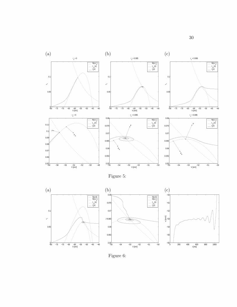
4-a where α > 0. We call P (rs) the fixed point of (8) corresponding to theleftmost intersection of the N(v; rs) with nullcline of rf . Note that with theshape of N(v; rs) as in Fig. 4-a, P (rs) moves to the right as rs increases.

We call rs,M the value of rs corresponding to the nullclines intersectingat the maximum of N(v, rs). In Fig. 4-a, α is very close to rs,M . We furtherassume that eqs. (8) have a subcritical (unstable) Hopf bifurcation point PH

at some value rs,H = rs,M + O(ε) close to the maximum of N(v; rs). Wealso assume that for each rs there is a point PB(rs) on the left branch ofrf = N(v; rs) (rs < rs,M), having the property that it separates those fixedpoints that are stable nodes from those that are stable spirals. In our model,without loss of generality, we are starting with rs = 0. For rs = 0, we assumePB(0) is to the right of P (0) and for rs = α, PB(α) is to the left of P (α);our analysis uses that. Our assumptions reproduce the conditions of the realmodel for the parameters of interest. Note that, in the real model, the resetof Ih due to a spike (see Section 3.2.2) brings the trajectory to the initialcondition rs = 0.

There is another value, rs,c, of rs at which the canard explosion occurs (inthe limit of ε → 0). This value is smaller than rs,H. Figure 4-b schematicallyshows the bifurcation diagram, including rs,H and rs,c, for a subcritical Hopfbifurcation. Note that the separation of scales in system (8) is necessary forthe existence of the canard explosion.

Figure 5 illustrates the three behaviors of the system for different valuesof rs in the presence of the above assumptions. In all three cases, we con-sider trajectories that first approach the v-nullcline and then stay close to it,moving slowly (Fig. 5-a). That there are such trajectories is a consequenceof the separation of time scales and the existence of an attracting invariantmanifold close to the nullcline. The trajectory we are interested in (comingfrom the end of a spike) has this property. For values of rs ≥ 0 such thatP (rs) is to the left of PB(rs), such trajectories approach the fixed point with-out oscillation; the attraction comes from the stability of the critical pointP (0). This is shown in (Figure 5-a).

For a value of rs > 0 such that P (rs) is to the right of PB(rs) but is stillstable, the critical point has trajectories spiraling inward. In this situation, asin the previous paragraph, the separation of time scales shapes the nature ofthe trajectories approaching the critical point. The trajectories now traverseacross the maximum of rf = N(v; rs) (Figure 5-b). There is still an invariantmanifold close to the v-nullcline, but its attractiveness changes (in the limitas ε goes to zero) to unstable to the right of the maximum. Nevertheless,

10

the trajectory stays close to that invariant manifold in the “top” part of eachspiral. This is what we refer to as the “canard structure”, and it is relatedto the mechanism by which small amplitude limit cycles blow up into largerelaxation ones.

For some value of rs still larger, the relevant trajectories do not spiralaround the maxima of the v-nullcline (Fig. 5-c). Instead, the trajectorymoves across the maximum, close to the unstable small amplitude limit cyclecreated in the subcritical Hopf bifurcation, and leaves its neighborhood. Notethat, in two dimensions, the requirement that trajectories do not cross eachother prevents them from spiraling in, as long as an unstable small amplitudelimit cycle surrounds the stable fixed point P (rs). For values of rs > rs,H thefixed point P (rs) changes from stable to unstable and there is no longer anunstable limit cycle. In principle, trajectories starting close enough to P (rs)spiral out and finally leave the N(v; rs) knee neighborhood. However, thetrajectories we are interested in have initial conditions far away from P (rs),and they approach the knee and leave its neighborhood without spiralingout.

In the above discussion, the separation of time scales was assumed, usingε � 1. In (4-5), this separation of scales during the ISI studied here isintrinsic to the system. It can be uncovered by defining ε = G−1

L = 0.025and rescaling the system t → ε t. We do not pursue this here. From (4-5)the v-nullcline is now given by

N(v; rs) =Iapp − Gp p∞(v) (v − ENa) − Gh 0.35 rs (v − Eh) − GL (v − EL)

Gh 0.65 (v − Eh).

(9)Equations (4-5) satisfy the hypotheses above: As rs is increased, N(v; rs)

moves downward (with a change of shape), and the leftmost critical pointP (rs) moves to the right. A standard stability analysis (not given here) showsthat, for the lowest values of rs, P (rs) is a stable node, as in Fig. 5-a. As rs

is increased, P (rs) becomes a stable focus (Fig 5-b). For a still larger value,the system undergoes a subcritical Hopf bifurcation in the neighborhood ofN(v; rs). At still larger values of rs, the trajectory leaves the neighborhoodof the nullcline without oscillations. Indeed, Fig. 5a-c were drawn from eqs.(4-5). For the full equations (1-3), leaving the neighborhood of the null-cline, with or without oscillations, corresponds to leaving the regime of the

11

reduced equations and going into a regime in which the spiking componentsare important.

The time spent in the oscillations (decaying or expanding) is closely re-lated to the time the trajectory of (4-6) spends in a subthreshold oscillation(STO). Thus, the canard structure, which forces the trajectory to stay closeto the invariant manifold at the “top” portion of the oscillations and imposesa time scale for the STO.

3.3.2 A three-dimensional approach: Generation of subthreshold

oscillations

Here we study system (4)-(6). τrf< τrs

and rs,∞(v) ∼ rf,∞(v) (see Fig. 1),so eq. (6) is slower than (5). The rescaling mentioned in Section 3.3.1 (notpresented here) confirms that. This is illustrated in Fig. 3 (the second panelis a blow up of the first one). It is evident, by comparing the last two panels,that rs evolves slower than rf at the beginning of the ISI. In the middle of theISI v and rf engage in a STO. rs evolves slowly and continues to increase.The assumption drs/dt � drf/dt is not satisfied, so the problem can notbe put in the slow passage problem framework used by other authors; e.g.Baer et al. (1989). However, the separation of scales is still large enoughto allow the study of the dynamics of eqs. (4)-(6) by looking at slowlyevolving phase planes for eqs. (4)-(5), each one corresponding to a constantvalue of rs. Three dimensional problems with one fast and two slow variableshave been treated using different approaches by other authors (Wechselberger2004; Drover et al. 2004). Here we focus on a heuristic explanation of themechanism of generation of STOs and the transition from STOs to spikes inthe reduced SC model.

The dynamics of the reduced system can be heuristically explained bylooking at phase planes of the type discussed in Section 3.3.1 continuouslyevolving with rs. We illustrate this in Fig. 6. The schematic Fig. 4-a ishelpful in this explanation too. As rs evolves, the v-nullcline N(v; rs) con-tinuously moves down, generating a two-dimensional slow manifold. P (rs),which is also continuously evolving, generates a curve (in Fig. 4-b this curvecontains the points P (0) and P (α) and it is contained in the rf -nullcline).There are two other relevant curves parametrized by rs, the fold curve L join-ing the maxima of N(v; rs) and the separatrix curve LB joining the pointsPB(rs) (not shown in the Figs.). As rs increases, rf,∞ intersects both L andLB. Note that by intersecting the nullsurface N(v; rs) with planes rs = k

12

(k > 0 constant) one recovers the nullclines N(v; k) corresponding to two-dimensional systems, as described in Section 3.3.1. Values of P (rs) to theleft of LB and close enough to LB correspond to stable foci in N(v; k), andfor some value of rs such that P (rs) is to the right of L, P (rs) is to the leftof the HB point. We use both two- and three-dimensional approaches in ourexplanation.

Due to the separation of time scales, the trajectory T starting at (v0, rf,0) =(−80, 0) stays close to the manifold N(v; rs) (Fenichel 1971) and movestowards P (rs). The 2D points P (rs) are not fixed points (in the three-dimensional view), so there is no convergence to them; they are target pointstowards which the trajectory moves. Note that the speed of rs in Fig. 3 isnot constant, but decreases as rs increases. When T gets close enough tothe knee of N(v; rs) and rs is such that P (rs) corresponds to a focus in atwo-dimensional view, T oscillates around the knee, staying close to the slowmanifold N(v; rs). In this two-dimensional view, this corresponds to “spi-raling down” to a fixed point. Note that T can get inside the “limit cycle”because of the extra dimension in the 3D system. As rs increases further,P (rs) is to the right of the HB point and the trajectory escapes this regimeto the spiking one, where INa and IK get activated. Note that the spike isproduced at almost the same voltage at which the previous STO reachedits maximum. That means that the phase of the STOs at which a spike isproduced is governed by the canard structure.

The amplitude of the oscillations decreases as P (rs) approaches the curveL (joining the maxima of N(v; rs)) and increases again for values of P (rs) tothe right of L. This is illustrated in Fig. 6 (see also Fig. 5 for a comparisonwith the two-dimensional case). Past the HB point, the unstable limit cyclehas disappeared, so there is no impediment to spiraling outwards in thelocally relevant 2D analogue.

The number and amplitude of the STOs is affected by the speed of rs:The slower rs, the more STOs are developed, since T spends more time nearthe knee. On the other hand, if rs evolves fast enough, T does not spendenough time near the knee for even one STO to be generated. In the reducedSC model, the speed of rs is not uniform but decreases with time (see Fig.3). To the first approximation, it is faster for values of rs < rs,M (P (rs) tothe left of the curve L) than for values of rs > rs,M . Thus, there may befewer STOs with decreasing amplitude. As a consequence the STOs withdecreasing amplitude are hard to see.

13

3.4 Robust subthreshold oscillations in a noisy GIF SC

model

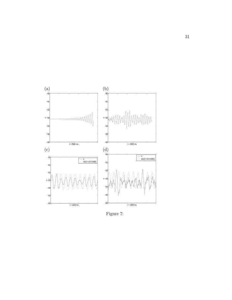
In Section 3.3 we explained the mechanism of generation of STOs for the re-duced SC model, which is deterministic. One of the features of deterministicSC models is that, for physiologically plausible parameters (and consequentspeeds of rs), STOs and mixed mode patterns are unlike those seen in ex-periments. If the STOs generated by the SC model do not decay to restingpotential, they increase their amplitude. Simulations show that an actionpotential is fired, as shown in Figs. 6-c and 7-a. In this case, the pattern re-peats itself at a roughly constant period. In experiments, however, when themembrane potential is depolarized from resting potential to a value belowspiking threshold, STOs at a theta frequency are generated with no apparentamplitude pattern. As the membrane potential approaches spiking threshold,SCs fire action potentials with no clear regular firing pattern. See Section 1for references.

Various modeling studies have introduced channel noise in order to ob-tain robust STOs. White et al. (1998) showed that the number of of per-sistent Na+ channels underlying STOs is relatively small and argued thatthe stochastic behavior of these channels may contribute crucially to thecellular-level responses. In their study they used a biophysical stochastic-deterministic model having INap and IKs in addition to the standard HHcurrents. The INap they used was represented by a population of stochasticion channels. Using this model they found regimes in which STOs and spikescoexist. More recently, Fransen et al. (2004) used a noisy model havingINap and a two-component Ih. They concluded that, although noise is notrequired for the SC to display STOs, its presence increases their robustness.

Here we want to explain how the effects of noise can be understood usingthe canard structure framework explained in previous sections. For this weintroduce channel white noise in INap. We do that in a very simple way, notclaiming it to be biophysically plausible, but simple enough to give a heuristicexplanation of the mechanism of generation of robust STOs due to noiseeffects. We add a stochastic term

√2 D η(t) to the dynamic equation for p.

This term is delta correlated with zero mean; i.e., < η(t), η(t′) >= δ(t − t′).D > 0 is the standard deviation. Since p is slaved to v, we substitutep∞(v) + τp(v)

√2 D η(t) for p∞(v) in in eq. (4).

In order to get results qualitatively similar to the findings of other authors(see Fransen et al. (2004), for an example) we set the value of the tonic drive

14

to I0app = −2.58, so that in the absence of noise the SC is silent but the

system is very close to PB(0) (see Fig. 4-a). In Fig. 7-a we show the voltagetrace for a noiseless system (D = 0) driven at Iapp = −2.55 > I0

app up to thetime where the first spike occurs. In Fig. 7-b we show the voltage trace forD = DM = 10−6 and I0

app. DM is approximately the largest value of D forwhich the SC displays only STOs in the time interval considered. For largervalues of D the SC fires at least one spike in this interval.

In Fig. 7-c we compare the voltage trace of the SC presented in Fig.7-b with a 10 Hz sinusoidal function to show that the noisy SC oscillates atapproximately this frequency. The power spectrum of the STOs in Fig. 7-band -c have a well defined peak at 10 Hz (data not shown).

If one chooses a lower value of Iapp (making the intersection point betweennullclines further to the left of PB(0)), one can still get STOs with a thetafrequency component provided the value of D is increased. Because of theincrease in D, the voltage traces look noisier than in the former case. Asan illustration, Fig. 7-d shows the voltage traces for Iapp = −2.7 and D =2.5 × 10−5. There the agreement with a 10 Hz sinusoidal function is not asgood as in the previous case discussed. The power spectrum for this casestill has a peak centered at 10 Hz but it is wider.

In all cases, as D decreases the frequency preference is kept, but theamplitude of the STOs decreases. Qualitatively similar results have beenobtained for other similar parameters regimes. In all cases considered, robustSTOs similar to the ones shown in Fig. 7-b were found, provided Iapp wasslightly lower than the boundary value PB(0) above which the fixed point isa stable focus.

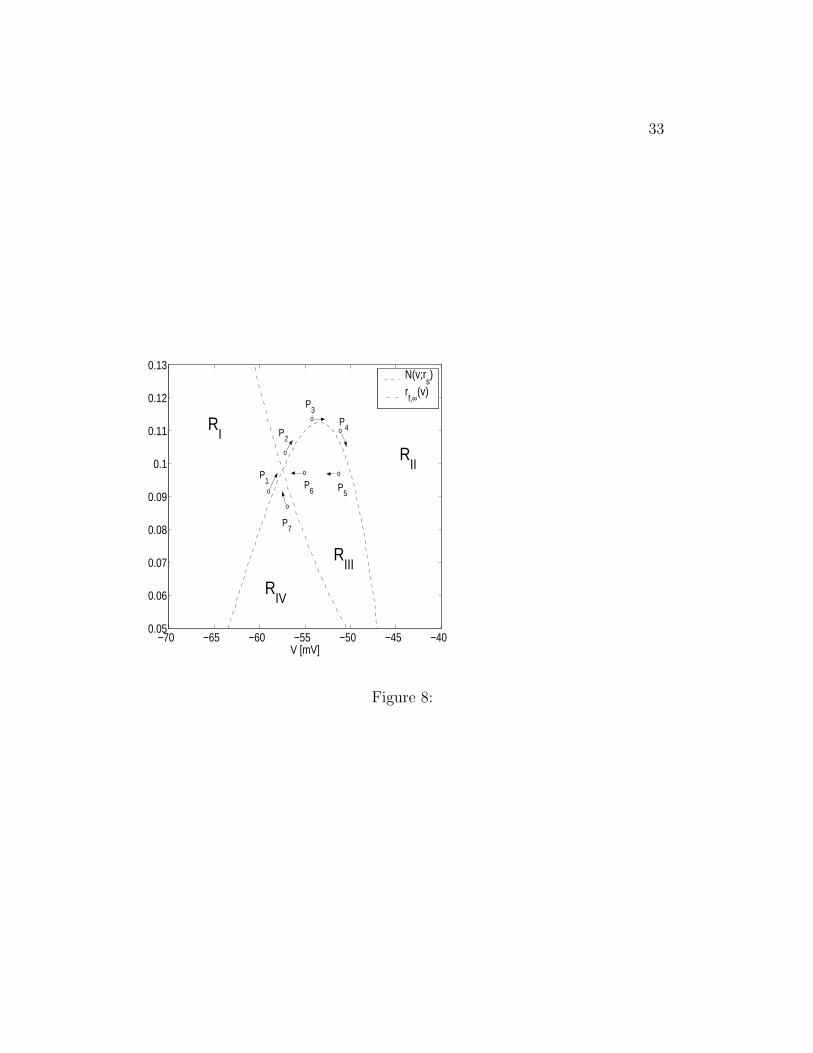
For the case described above, a heuristic explanation of the effect of noisecan be achieved by using the canard structure framework described in formersections. As before we view the dynamics of the three dimensional system asa two-dimensional system with rs moving the v-nullcline N(v; rs) downwards.In the absence of noise, the intersection of N(v; rs) and rf,∞(v) determinefour regions inside which the trajectory T evolves, as schematically shown inFig. 8, targeting the 2-D fixed point in a monotonic or oscillatory way. Theeffect of noise is to randomly move N(v; rs) and consequently, to randomlymove the “fixed point” (intersection between nullclines). As this happens,the tip of the trajectory, P(t) may find itself in any of the four regions.For as long as this situation persists, T evolves, targeting the fixed point asschematically shown in Fig. 8.

A distinguished situation occurs when T is in RII . In this case, T is

15

forced to move around the knee of N(v; rs) before crossing N(v; rs) to RIII .In this way an oscillation is obtained with a similar frequency to its noiselesscounterpart. It may occur that, before finishing the oscillation, η(t) is largeenough to move N(v; rs) up, leaving T in RII , and this effect lasts for enoughtime so to prevent the oscillation. However, for small enough values of D,the probability that this happens is very low. So once T is in RII it willproduce a STO with high probability and at the frequency established bythe canard structure. For values of D larger than some DM , the noisy SCwill produce a spike in a given time interval for which there are no spikeswhen D = DM . For very small values of D (D < DM), one gets STOs withthe same frequency content as for D = DM but with smaller amplitude.

If the parameters of the model are such that N(v; rs) and rf,∞(v) intersectat a stable node below and not very close to PB, then one needs a larger valueof D (than in the case described in the former paragraph) for T to get to theknee of N(v; rs) where, due to the canard structure, one get STOs. In thiscase the STOs will look very noisy.

3.5 Synchronization properties of networks of GIF SC

models

It has been argued that Ih plays a relevant role in determining the synchro-nization properties of networks including SCs and other cells having similarelectric properties (Acker et al. 2003; Netoff et al. 2004; Rotstein et al. 2004;Jalics et al. 2004). Among the latter we mention the oriens lacunosum-moleculare (O-LM) cells in the hippocampus (Gillies et al. 2002). Since theeffects of Ih are captured by the GIF SC model, we use equations (4,6,7)instead of the full SC model in our network synchronization studies andcompare our results with previous findings.

To consider the effect of synaptic currents to each SC we add a synapticterm −IS to the current-balance equation (4)

CdV

dt= Iapp − Gp p∞(V ) (V − ENa) − IL − Ih − IS (10)

where IS = GS S (v−Erev) and Erev = Eex = 0 mV or Erev = Ein = −80 mV ,for excitatory or inhibitory synaptic connections respectively. The synapticvariable S we used is given by (Dayan and Abbott 2001)

16

S = SN (e−t/τ1−e−t/τ2), with SN =

[

(

τ2

τ1

)τrise/τ1

−(

τ2

τ1

)τrise/τ2]

−1

.

(11)We define the decay time τdec as the time it takes S to decay from its

maximum value to 0.37 % (1/e) of its maximum value. Below, the units ofτ1, τ2 and τdec are msec, and the units of GS are mS/cm2. We performedsimulations for different natural frequencies of the SCs in the theta range(8 - 12 Hz). The natural frequency of a cell is its firing frequency whenuncoupled.

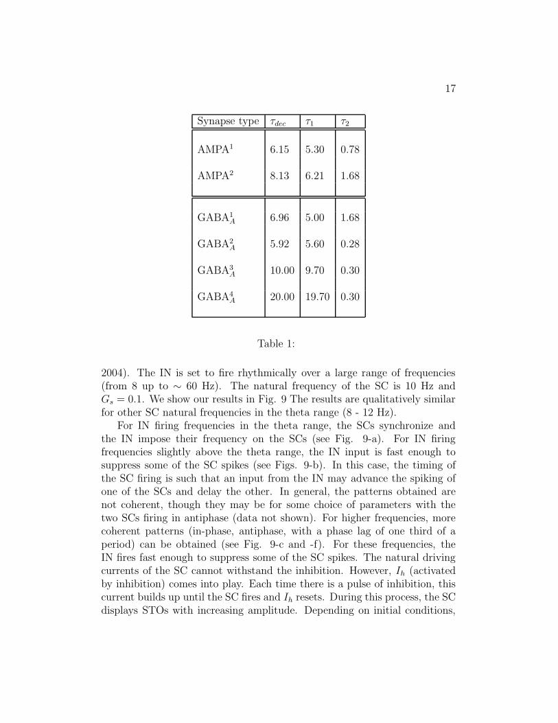
We consider different types of networks in which excitatory and/or in-hibitory connections are present. SCs are excitatory and they are connectedvia AMPA. The SC full model has been used for O-LM cells in the hip-pocampus (Rotstein et al. 2004). In contrast to the SCs, O-LM cells areinhibitory mediated by GABAA as are other inhibitory neurons (IN) presentin excitatory/inhibitory networks including SCs. We used various kinet-ics for both AMPA and GABAA summarized in Table 1. The AMPA1 andAMPA2 kinetics have been considered by Acker et al. (2003) and Netoff et al.(2004) respectively. The GABA1

A kinetics has been considered by Netoff et al.(2004). The GABA2

A kinetics is standard (Destexhe et al. 1994; Dayan andAbbott 2001) and then worth considering, but has not been used in networksincluding SCs. The GABA3

A and GABA4A kinetics correspond to values used

by Rotstein et al. (2004) for O-LM cells.Our simulations show that two SCs connected via AMPA1 and AMPA2

synchronize at theta frequencies for values of GS up to ∼ 0.089 and ∼ 0.065respectively and natural frequencies of 12 Hz. For higher values of GS thenetworks fire in antiphase at a much higher frequency (∼ 50 to 60) Hz. Theresults are qualitatively similar for SC natural frequencies in the 8 - 12 Hzrange. All this is consistent with the findings by Acker et al. (2003) and theresults obtained using the full SC model.

Simulations of SCs connected via inhibition using the four values for theGABAA kinetics (see Table 1) show that for physiological values of GS, thenetworks displayed an antiphase firing pattern as predicted experimentallyand theoretically (Netoff et al. 2003; Rotstein et al. 2004).

To study the effect of common inhibition on two uncoupled SCs we con-nect an interneuron (IN), using a standard Hodgkin-Huxley model, to thetwo SCs using GABA1

A synaptic connections (see Table 1) as in (Netoff et al.

17

Synapse type τdec τ1 τ2

AMPA1 6.15 5.30 0.78

AMPA2 8.13 6.21 1.68

GABA1A 6.96 5.00 1.68

GABA2A 5.92 5.60 0.28

GABA3A 10.00 9.70 0.30

GABA4A 20.00 19.70 0.30

Table 1:

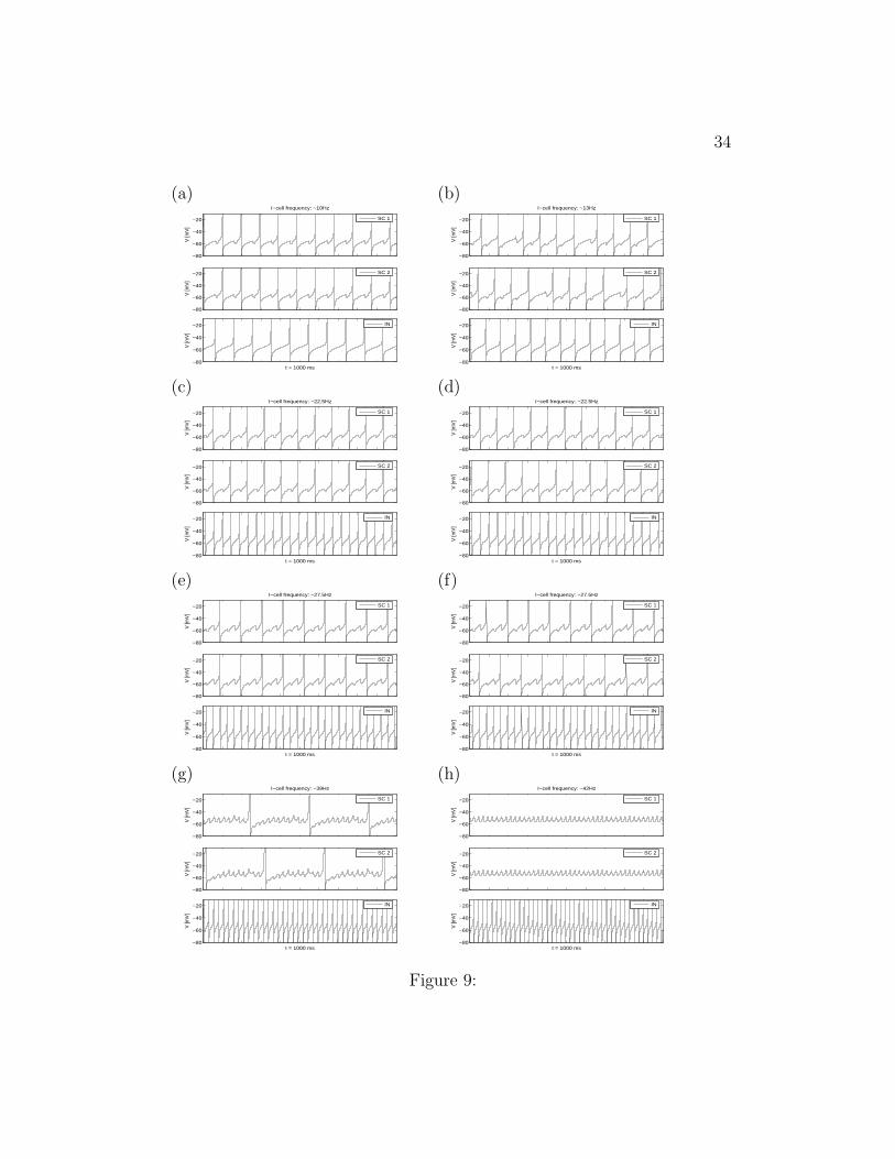
2004). The IN is set to fire rhythmically over a large range of frequencies(from 8 up to ∼ 60 Hz). The natural frequency of the SC is 10 Hz andGs = 0.1. We show our results in Fig. 9 The results are qualitatively similarfor other SC natural frequencies in the theta range (8 - 12 Hz).

For IN firing frequencies in the theta range, the SCs synchronize andthe IN impose their frequency on the SCs (see Fig. 9-a). For IN firingfrequencies slightly above the theta range, the IN input is fast enough tosuppress some of the SC spikes (see Figs. 9-b). In this case, the timing ofthe SC firing is such that an input from the IN may advance the spiking ofone of the SCs and delay the other. In general, the patterns obtained arenot coherent, though they may be for some choice of parameters with thetwo SCs firing in antiphase (data not shown). For higher frequencies, morecoherent patterns (in-phase, antiphase, with a phase lag of one third of aperiod) can be obtained (see Fig. 9-c and -f). For these frequencies, theIN fires fast enough to suppress some of the SC spikes. The natural drivingcurrents of the SC cannot withstand the inhibition. However, Ih (activatedby inhibition) comes into play. Each time there is a pulse of inhibition, thiscurrent builds up until the SC fires and Ih resets. During this process, the SCdisplays STOs with increasing amplitude. Depending on initial conditions,

18

SC may phase-lock to different cycles of the IN, resulting in the patternsshown in Figs. 9-c to -f. Note that in Figs. 9-c and -d the SC frequency ishalf the IN frequency (1 STO per spike) while in Figs. 9-e and -f, the SCfrequency is a third of the IN frequency (2 STOs per spike). In the lattercase, the IN frequency is too high for the SC to overcome inhibition in onlyone cycle; i.e., after the SC fires the IN hits the SC twice before the Ih buildsup and allows the SC to fire again.

As the IN frequency increases, the number of STOs per spike also in-creases (Figs.9-c to g); it takes an increasing number of cycles for the h-current to build up enough to overcome the inhibition (Kopell and LeMasson1994). For IN firing at ∼ 42 Hz, the SC firing is completely suppresed; i.e.the h-current is not able to increase to high enough values as to allow the SCvoltage to reach threshold (Fig.9-h). This qualitatively matches simulationsdone with similar equations (Rotstein et al. 2004).

4 Discussion

Subthreshold membrane potential oscillations have been observed at vari-ous locations in the brain (Alonso and Llinas 1989; Dickson et al. 2000b;Hutcheon et al. 1996; Llinas and Yarom 1981, 1986; Erchova et al. 2004).In the last years, the study of STOs in the MEC has received special atten-tion from both the experimental and theoretical point of view (see referencesin Section 1). The results presented in this manuscript contribute to theunderstanding of the biophysical mechanism of this phenomenon.

It was already known that the interaction between INap and Ih is enoughto account for the generation of STOs in layer II of the MEC. However, thespecific role of each one of these currents, in particular, the fast and slowcomponents of Ih, and the dynamics of their interaction, was not yet under-stood. To answer these questions we looked at a biophysical single-cell modelthat has been used in the past to study synchronization properties of SCs.We demonstrated that this seven-dimensional model can be approximatedby a reduced three-dimensional model in the ISI, where STOs are observed.This approximation is based on the fact that the spiking generation currents(INa and IK) are not active in the ISI regime. Furthermore, there is a clearseparation of scales between the three dynamic variables. This, together withthe arrangement of the nullsurfaces in the three-dimensional phase space cre-ates what we call the canard structure. This structure serves as the basic

19

framework to understand the dynamic aspects of the generation of STOsand the coexistence of STOs and spikes. In the absence of rs as a dynamicvariable, the v and rf nullclines intersect at a fixed point that is a stablenode, stable focus or unstable focus. Thus, trajectories can either convergeto a fixed point (in an oscillatory fashion or not) or spike. No mixed-modesare possible. The role of rs, evolving on the slowest time scale of the system,is, roughly speaking, to serve as a bridge between both dynamic behaviors,allowing for coexistence of STOs and spikes. Each time a trajectory movesaround the knee it has to “decide” whether to cross the v nullcline or escapethe subthreshold regime, producing a STO or a spike respectively. The valueof v at which this happens is the one corresponding the peak of a STO. So,the canard structure approach explains why spikes occurs at the peak of theSTOs, as experimentally found (Dickson et al. 2000b).

The structural dynamic ideas presented here are consistent with previoustheoretical observations by (Fransen et al. 2004) who concluded that the fastcomponent is the major factor in the oscillation generation. Simulation of thepartial blockade (65%) of Ih by cesium caused a decrease in the amplitude andfrequency of STOs corresponding to that observed in current-clamp record-ings. Full block of Ih completely abolished the oscillations. These findingscan be explained in terms of the canard structure discussed here. Our calcu-lations show that blockade (partial or total) of Ih has the effect of changingthe voltage nullcline N(v; rs) in such a way that either the knee disappears orthe stable fixed point P (0) is farther away from the knee, requiring a quickertime scale for rs or a larger value of Gh to be able to reach the STO regime(associated with this knee). We develop these ideas further in a future paper.

The patterns of activity seen in experiments are very irregular, in contrastto the regular patterns (a constant number of STOs per spike) obtained inour deterministic SC model. In terms of the canard mechanism proposed inthis paper, the occurrence of a spike can be thought of as a loss of stability ofthe STO regime (a spiking instability). In related theoretical work, stochas-tic models, with persistent sodium channel noise, have been succesfully usedto enhance the robustness of STOs (White et al. 1998). In Section 3.4 weobtained the same result in our GIF SC model and we identified conditionsunder which the STOs are very close to a sinusoidal function. One poten-tial explanation for the effect of noise in enhancing the robustness of STOsmight be that noise suppresses spikes; i.e., noise prevents spiking by movingthe voltage nullcline in a way that forces the trajectory to stay away fromthe spiking instability. However, our theoretical approach (using the canard

20

structure) suggests that this is not the case. The most robust STOs areobtained when, in the absence of noise, the SC is silent but close to STOactivity. The effect of noise is to force the system to move around the kneeof the voltage nullcline, thus creating a STO. In this sense, noise creates an“intermediate STO state” in between silence and STO/spiking. Once thetrajectory moves around the knee the effect of noise is minimal. If the noiseamplitude (D) is too big, a spike can be produced. Otherwise, the trajectoryreturns to the fixed point where noise becomes important again and can drivethe trajectory to a new STO excursion.

The function of STOs is not clear yet, but they are believed by some toplay a role in synchronization and other coherent dynamic behavior (Hutcheonand Yarom 2000; Dickson et al. 2000a; Buzsaki and Draguhn 2004). We stud-ied the synchronization properties of networks including SCs using the GIFpresented in Section 3.2.3. Our results are qualitatively similar to otherstudies that used the full SC model (Acker et al. 2003; Netoff et al. 2004;Rotstein et al. 2004; Pervouchine et al. 2004). We hypothesize that the ca-nard structure, created by the same equations used in the GIF SC model, isresponsible for the dynamics producing the coherent behaviour, rather thanthe existence of STOs per se.

Problems with similar mathematical structure as the one given by eqs.(4)-(6) have been studied by Wechselberger (2004) and Drover et al. (2004) inorder to explain the spike-frequency reduction of a Hodgkin-Huxley neurondue to excitatory synaptic self-coupling. In both cases, a two-dimensionalsystem with fast (V) and slow (h) variables was used to model the dynamicsof the neuron, and an extra slow variable was used for an autapse on theneuron. The two approaches are different but complementary. The reduc-tion of spiking frequency is the result of the trajectory beings trapped in aneighborhood of a fold line (L in our notation). As in our model, STOs (orMMOs) are observed in a neighborhood of L. However, in the SC model, theSTOs are intrinsically generated by the single cell with no need of a synapticself-coupling.

In this work we give heuristic arguments to explain the generation of STOsin the SC model. Work in progress, including the development of reductionof dimension techniques (Rotstein et al. 2005) and the application of thetheory developed by Wechselberger (2004), aims to make the justifications ofthe reductions to the GIF model and the generation of STOs more precise.

.

21

Acknowledgments

The authors want to Andreas Herz, Steve Epstein and Carson Chow forfruitful discussions.

This work was partially supported by the Burroughs Wellcome Fund(HGR), NIH grant 5 RO1 NS46058 (NK), NSF grant DMS-0211505 (NK)and the graduate program “Dynamics and Evolution of Cellular and Macro-molecular Processes” of the German Research Foundation, DFG (TO).

References

Acker CD, Kopell N, and White JA, Synchronization of strongly cou-pled excitatory neurons: relating network behavior to biophysics. Journal

of Computational Neuroscience 15: 71–90, 2003.

Alonso AA and Klink R, Differential electroresponsiveness of stellate andpyramidal-like cells of medial entorhinal cortex layer II. J Neurophysiol 70:144–157, 1993.

Alonso AA and Llinas RR, Subthreshold Na+-dependent theta like rhyth-micity in stellate cells of entorhinal cortex layer II. NATURE 342: 175–177,1989.

Baer SM, Erneux T, and Rinzel J, The slow passage through a Hopfbifurcation: delay, memory effects, and resonance. SIAM J Appl Math 49:55–71, 1989.

Burden RL and Faires JD, Numerical analysis. PWS Publishing Com-pany - Boston, 1980.

Buzsaki G and Draguhn, Neuronal oscillations in cortical networks. Sci-

ence 304: 1926–1929, 2004.

Chow CC and White JA, Spontaneous action potentials due to channelfluctuation. Biophysical J 71: 3013–3021, 1996.

Dayan P and Abbott LF, Theoretical Neuroscience. The MIT Press, 2001.

22

Destexhe A, Mainen ZF, and Sejnowski TJ, Synthesis of models forexcitable membranes, synaptic transmission and neuromodulation using acommon kinetic formalism 3: 195–230, 1994.

Dickson CT, Magistretti J, Shalinsky M, Hamam B, and Alonso

AA, Oscillatory activity in entorhinal neurons and circuits. Ann NY Acad

Sci 911: 127–150, 2000a.

Dickson CT, Magistretti J, Shalinsky MH, Fransen E, Hasselmo M,

and Alonso AA, Properties and role of Ih in the pacing of subthresholdoscillation in entorhinal cortex layer II neurons. J Neurophysiol 83: 2562–2579, 2000b.

Drover J, Rubin J, Su J, and Ermentrout B, Analysis of a canardmechanism by which excitatory synaptic coupling can synchronize neuronsat low firing frequencies. SIAM J Appl Math, to appear 2004.

Dumortier F and Roussarie R, Canard cycles and center manifolds. Mem-

oirs of the American Mathematical Society 121 (577), 1996.

Eckhaus W, Relaxation oscillations including a standard chase on frenchducks. In Lecture Notes in Mathematics, Springer-Verlag 985: 449–497,1983.

Erchova I, Kreck G, Heinemann U, and Herz AVM, Dynamics ofrat entorhinal cortex layer II and III cells: characteristics of membranepotential resonance ar rest predict oscillation properties near threshold. J

Physiol 560: 89–110, 2004.

Fenichel N, Persistence and smoothness of invariant manifolds for flows.Ind Univ Math J 21: 193–225, 1971.

Fransen E, Alonso AA, Dickson CT, and Magistretti ME J Has-

selmo, Ionic mechanisms in the generation of subthreshold oscillationsand action potential clustering in entorhinal layer ii stellate neurons. Hip-

pocampus 14: 368–384, 2004.

Fransen E, Dickson CT, Magistretti J, Alonso AA, and Hasselmo

ME, Modeling the generation of subthreshold membrane potential oscil-lations of entorhinal cortex layer II stellate cells. Soc Neurosci Abstr 24:814.815, 1998.

23

Fransen E, Wallestein GV, Alonso AA, Dickson CT, and Hasselmo

ME, A biophysical simulation of intrinsic and network properties of en-torhinal cortex. Neurocomputing 26-27: 375–380, 1999.

Gillies MJ, Traub RD, LeBeau FEN, Davies CH, Gloveli T, Buhl

EH, and Whittington MA, A model of atropine-resistant theta oscil-lations in rat hippocampal area CA1. J Physiol 543.3: 779–793, 2002.

Hutcheon B, Miura RM, and Puil E, Subthreshold membrane resonancein neocortical neurons. J Neurophysiol 76: 683–697, 1996.

Hutcheon B and Yarom Y, Resonance oscillations and the intrinsic fre-quency preferences in neurons. Trends Neurosci 23: 216–222, 2000.

Izhikevich EM, Resonate-and-fire neurons. Neural Networks 14: 883–894,2001.

Jalics J, Kispersky T, Dickson C, and Kopell N, Neuronal ensemblesand modules: modeling dynamics in medial entorhinal cortex. Society for

Neuroscience Abstracts 517.1, 2004.

Klink RM and Alonso A, Ionic mechanisms for the subthreshold oscil-lations and differential electroresponsiveness of medial entorhinal cortexlayer II neurons. J Neurophysiol 70: 128–143, 1993.

Klink RM and Alonso AA, Ionic mechanisms of muscarinic depolarizationin entorhinal cortex layer ii neurons. J Neurophysiol 77: 1829–1843, 1997.

Kopell N and LeMasson G, Rhythmogenesis, amplitude modulation, andmultiplexing in a cortical architecture. Proc Natl Acad Sci USA 91: 10586–10590, 1994.

Krupa M and Szmolyan P, Relaxation oscillation and canard explosion.J Diff Eq 174: 312–368, 2001.

Llinas RR and Yarom Y, Electrophysiology of mammalian inferior olivaryneurons in vitro. different types of voltage-dependent ionic conductances.J Physiol 315: 549–567, 1981.

Llinas RR and Yarom Y, Oscillatory properties of guinea pig olivary neu-rons and their pharmachological modulation: an in vitro study. J Physiol

376: 163–182, 1986.

24

Magistretti J and Alonso AA, Biophysical properties and slow valtage-dependent inactivation of a sustained sodium current in entorhinal cortexlayer-II principal neurons. a whole-cell and single-channel study. J Gen

Physiol 114(4): 491–509, 1999.

Magistretti J and Ragsdale DS, High conductance sustained single-channel activity responsible for the low-threshold persistent Na+ currentin entorhinal cortex neurons. J Neurosci 19(17): 7334–7341, 1999.

Makarov VA, Nekorkin VI, and Velarde MG, Spiking behavior in anoise-driven system combining oscillatory and excitatory properties. Phys

Rev Lett 15: 3031–3034, 2001.

Netoff T, Banks M, and White J, Bridging single cell and networkdynamics. Society for Neuroscience Abstracts 32 171.7, 2003.

Netoff T, Pervouchine D, Kopell N, and White J, Oscillation fre-quency switches in model and hybrid networks of the hippocampus. Society

for Neuroscience Abstracts *32*, In press 2004.

Pervouchine D, others, and Kopell N. In preparation 2004.

Richardson MJE, Brunel N, and Hakim V, From subthreshold to firing-rate resonance. J Neurophysiol 89: 2538–2554, 2003.

Rotstein HG, Clewley R, Wechselberger M, and Kopell N, Dynamicsof an entorhinal cortex stellate cell model. In preparation 2005.

Rotstein HG, Pervouchine D, Gillies MJ, Acker CD, White JA,

Buhl EH, Whittington MA, and Kopell N, Slow and fast inhibi-tion and h-current interact to create a theta rhythm in a model of ca1interneuron networks. Submitted 2004.

Wechselberger M, Existence and bifurcation of canards in R3 in the caseof a folded node. SIAM J Appl Dyn Syst, to appear 2004.

White JA, Budde T, and Kay ARA, A bifurcation analysis of neuronalsubthreshold oscillations. Biophysical J 69: 1203–1217, 1995.

White JA, Klink R, Alonso A, and Kay ARA, Noise from voltage-gatedion channels may influence neuronal dynamics in the entorhinal cortex. J

Neurophysiol 80: 262–269, 1998.

25

White JA, Rubinstein JT, and Kay AA, Channel noise in neurons.Trends Neurosci 23(3): 131–137, 2000.

Table Legends

Table 1: Parameters and decay times (τdec) for synaptic connections ofvarious kinetic types (AMPA and GABAA). The units of τ1, τ2 and τdec aremsec.

Figure Legends

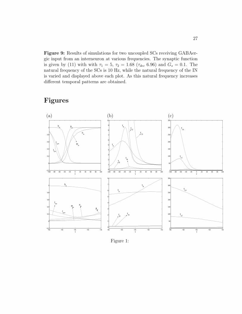
Figure 1: Ion channel dynamics for the full SC model (1-3). The gatingvariables are x = m, n, h, p, rf , rs. The bottom pannels are magnificationsof the top ones in the voltage interval (using mV units) (−65 : −40). (a)Activation and inactivation curves (x∞(V )) for the gating variables. (b)Voltage-dependent times scales (τx(V )) for the gating variables. The separa-tion of time-scales is clearly visible. Both, τr,f and τr,s evolve on time scalesmuch slower than the other variables. (c) Voltage dependent time scales ina larger time interval.

Figure 2: Changing Iapp changes the ratio of spikes to STOs in the fullSC model. Voltage (V ) traces, Ih and INap for various values of the appliedcurrent Iapp and Gh = 1.5. The values of the other parameters used in thesimulations are given in the Appendix. The second row in each panel is amagnification of the first row.

Figure 3: Gating variables during STOs and spikes in the full SC model.Voltage (V ), rf and rs traces for Iapp = −2.5 and Gh = 1.5. The values ofthe other parameters used in the simulations are given in the Appendix. Thesecond row is a magnification of the first row.

Figure 4: (a) Schematic representation of the nullclines N(v; rs) and rf,∞(v)of system (8) for rs = 0 and rs = α > 0. P (rs) represent fixed points, PB(rs)represent points dividing between stable nodes and foci. As α increases thenullcline N(v; rs moves down while the activation curve (nullcline) rf,∞(v)remains unchanged. (b) Schematic bifurcation diagram for a subcritical Hopf

26

bifurcation. An unstable limit cycle is born at the Hopf bifurcation point rs,H

out of a fixed point. This fixed point is stable to the left of rs,H , and unstable(to the right of rs,H). At the canard critical point rs,c the amplitude of thelimit cycle explodes.

Figure 5: Phase plane for the reduced SC model for various values of rs forGh = 1.5 and Iapp = −2.5. The values of the other parameters used in thesimulations are given in the Appendix. Lower panels are magnifications ofthe upper ones. (a) rs = 0: the trajectory converges to a fixed point withoutspiraling. (b) rs = 0.085: the trajectory spirals down to a fixed point. (c)rs = 0.086: the trajectory moves around the knee of the nullcline N(v; rs)and escapes the regime without spiraling.

Figure 6: Dynamics of the reduced SC model for Gh = 1.5 and Iapp = −2.5.The values of the other parameter used in the simulations are given in theAppendix. (a) Trajectory for rf and v when rs evolves continuously. (b)Magnification of panel (a). Note that when the trajectory escapes the regime(corresponding to the SC firing an action potential), it does so at the samevoltage at which the previous STO reached its maximum. (c) voltage trace.

Figure 7: Results of simulations for noiseless and noisy systems for Gh =1.5. The values of the parameter used in the simulations are given in theAppendix. (a) D = 0 and Iapp = −2.55. In the absence of noise the amplitudeof the STOs increase uniformly with time and eventually the SC fires anaction potential. In the figure we show the STOs up until the first spike. ForIapp = −2.58 and D = 0 the SC is silent (data not shown). (b) D = 10−6

and Iapp = −2.58. STOs are produced in the presence of noise, but theamplitude does not increase uniformly with time. For comparison we showthe STOs for the same amount of time as in Fig. (a). (c) D = 10−6 andIapp = −2.58. Comparison of the STOs produced in the noiseless case with asinusoidal function (10 Hz). (d) D = 2.5−5 and Iapp = −2.7. Comparison ofthe STOs produced in the noiseless case with a sinusoidal function (10 Hz).The value of D is larger as compared to the one in (c) and the STOs aremore influenced by noise.

Figure 8: Schematic diagram of the nullclines N(v; rs) and rf,∞(v). The ar-rows show the direction of motion of trajectories. In particular, perturbationsto the fixed point evolve in following the arrows.

27

Figure 9: Results of simulations for two uncoupled SCs receiving GABAer-gic input from an interneuron at various frequencies. The synaptic functionis given by (11) with with τ1 = 5, τ2 = 1.68 (τdec 6.96) and Gs = 0.1. Thenatural frequency of the SCs is 10 Hz, while the natural frequency of the INis varied and displayed above each plot. As this natural frequency increasesdifferent temporal patterns are obtained.

Figures

(a) (b) (c)

−100 −80 −60 −40 −20 0 20 40 60 80 100−0.2

0

0.2

0.4

0.6

0.8

1

v

h∞

rs,∞

rf,∞

p∞

n∞

m∞

−100 −80 −60 −40 −20 0 20 40 60 80 1000

1

2

3

4

5

6

7

8

9

10

v

τm

τ

p

τn

τh

τr,f

τr,s

−100 −80 −60 −40 −20 0 20 40 60 80 1000

50

100

150

200

250

300

350

v

τr,f

τr,s

−65 −60 −55 −50 −45−0.2

0

0.2

0.4

0.6

0.8

1

v

h∞

p∞ n∞ m∞

rs,∞

rf,∞

−65 −60 −55 −50 −45

0

1

2

3

4

5

6

7

8

v

τh

τn

τp τ

m

−65 −60 −55 −50 −450

50

100

150

200

250

300

350

v

τr,f

τr,s

Figure 1:

28

(a) (b)

−100−50

050

V [

mV

]

Iapp

=−2.51

−60

−55

−50

V [

mV

]

3

3.5

4

− I

h

4

6

t = 1000 ms

− I

Na

p

−100−50

050

V [

mV

]

Iapp

=−2.5

−60

−55

−50

V [

mV

]

3

3.5

4−

Ih

4

6

t = 1000 ms

− I

Na

p

(c) (d)

−100−50

050

V [

mV

]

Iapp

=−2.43

−60

−55

−50

V [

mV

]

3

3.5

4

− I

h

4

6

t = 1000 ms

− I

Na

p

−100−50

050

V [

mV

]

Iapp

=−2.42

−60

−55

−50

V [

mV

]

3

3.5

4

− I

h

4

6

t = 1000 ms

− I

Na

p

Figure 2:

29

−100−50

050

V [m

V]

−60

−55

−50

V [m

V]

0

0.05

0.1

0

0.05

0.1

t = 1000 ms

rf

rs

Figure 3:

(a) (b)

v

N(v;0)N(v;α)rf,∞

(v)

P(0)

PB(0)

P(α)

PB(α)

o

o

o o

rs

Am

plit

ud

e

unstablestable

rs,H

rs,c

0

Figure 4:

30

(a) (b) (c)

−80 −75 −70 −65 −60 −55 −50 −45 −400

0.05

0.1

V [mV]

rs = 0

r f

N(v;rs)

rf,∞

(v)rf(v)

−80 −75 −70 −65 −60 −55 −50 −45 −400

0.05

0.1

V [mV]

rs = 0.085

r f

N(v;rs)

rf,∞

(v)rf(v)

−80 −75 −70 −65 −60 −55 −50 −45 −400

0.05

0.1

V [mV]

rs = 0.086

r f

N(v;rs)

rf,∞

(v)rf(v)

−60 −58 −56 −54 −52 −50 −480.05

0.06

0.07

0.08

0.09

0.1

0.11

V [mV]

rs = 0

N(v;rs)

rf,∞

(v)rf(v)

P

PB

o

o

−55 −54 −53 −52 −51 −500.05

0.055

0.06

0.065

0.07

0.075

0.08

V [mV]

rs = 0.085

N(v;rs)

rf,∞

(v)rf(v)P

PB

o

−55 −54 −53 −52 −51 −500.05

0.055

0.06

0.065

0.07

0.075

0.08

V [mV]

rs = 0.086

N(v;rs)

rf,∞

(v)rf(v)

o

P

o

PB

Figure 5:

(a) (b) (c)

−80 −75 −70 −65 −60 −55 −50 −45 −400

0.05

0.1

V [mV]

r f

N(v;0)N(v;r

s)

rf,∞

(v)rf(v)

−55 −54 −53 −52 −51 −500.05

0.055

0.06

0.065

0.07

0.075

0.08

V [mV]

r f

N(v;0)N(v;r

s)

rf,∞

(v)rf(v)

0 200 400 600 800 1000−56

−55

−54

−53

−52

−51

−50

t [ms]

v [

mV

]

Figure 6:

31

(a) (b)

−56

−55

−54

−53

−52

−51

−50

t = 2500 ms

v

−56

−55

−54

−53

−52

−51

−50

t = 2500 ms

v

(c) (d)

−56

−55

−54

−53

−52

−51

−50

t = 1000 ms

v

vsin(2 π 10 t/1000)

−56

−55

−54

−53

−52

−51

−50

t = 1000 ms

v

vsin(2 π 10 t/1000)

Figure 7:

32

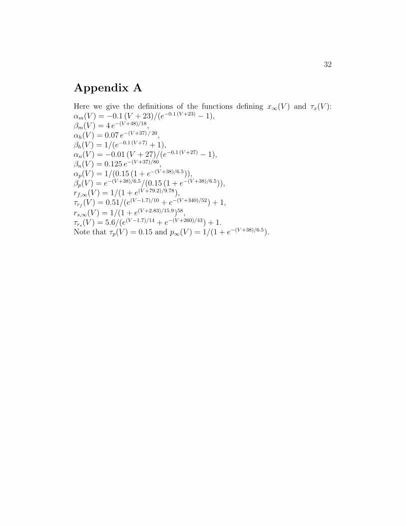
Appendix A

Here we give the definitions of the functions defining x∞(V ) and τx(V ):αm(V ) = −0.1 (V + 23)/(e−0.1 (V +23) − 1),βm(V ) = 4 e−(V +48)/18,αh(V ) = 0.07 e−(V +37) / 20,βh(V ) = 1/(e−0.1 (V +7) + 1),αn(V ) = −0.01 (V + 27)/(e−0.1 (V +27) − 1),βn(V ) = 0.125 e−(V +37)/80,αp(V ) = 1/(0.15 (1 + e−(V +38)/6.5)),βp(V ) = e−(V +38)/6.5/(0.15 (1 + e−(V +38)/6.5)),rf,∞(V ) = 1/(1 + e(V +79.2)/9.78),τrf

(V ) = 0.51/(e(V −1.7)/10 + e−(V +340)/52) + 1,

rs,∞(V ) = 1/(1 + e(V +2.83)/15.9)58,τrs

(V ) = 5.6/(e(V −1.7)/14 + e−(V +260)/43) + 1.Note that τp(V ) = 0.15 and p∞(V ) = 1/(1 + e−(V +38)/6.5).

33

−70 −65 −60 −55 −50 −45 −400.05

0.06

0.07

0.08

0.09

0.1

0.11

0.12

0.13

V [mV]

N(v;rs)

rf,∞

(v)

o

o

o

o

o

RI

RII

RIII

RIV

P1

P2

P3

P4

P5

o

P6

o

P7

Figure 8:

34

(a) (b)

−80

−60

−40

−20

I−cell frequency: ~10Hz

V [m

V]

−80

−60

−40

−20

V [m

V]

−80

−60

−40

−20

t = 1000 ms

V [m

V]

SC 1

SC 2

IN

−80

−60

−40

−20

I−cell frequency: ~13Hz

V [m

V]

−80

−60

−40

−20

V [m

V]

−80

−60

−40

−20

t = 1000 ms

V [m

V]

SC 1

SC 2

IN

(c) (d)

−80

−60

−40

−20

I−cell frequency: ~22.5Hz

V [m

V]

−80

−60

−40

−20

V [m

V]

−80

−60

−40

−20

t = 1000 ms

V [m

V]

SC 1

SC 2

IN

−80

−60

−40

−20

I−cell frequency: ~22.5Hz

V [m

V]

−80

−60

−40

−20

V [m

V]

−80

−60

−40

−20

t = 1000 ms

V [m

V]

SC 1

SC 2

IN

(e) (f)

−80

−60

−40

−20

I−cell frequency: ~27.5Hz

V [m

V]

−80

−60

−40

−20

V [m

V]

−80

−60

−40

−20

t = 1000 ms

V [m

V]

SC 1

SC 2

IN

−80

−60

−40

−20

I−cell frequency: ~27.5Hz

V [m

V]

−80

−60

−40

−20

V [m

V]

−80

−60

−40

−20

t = 1000 ms

V [m

V]

SC 1

SC 2

IN

(g) (h)

−80

−60

−40

−20

I−cell frequency: ~39Hz

V [m

V]

−80

−60

−40

−20

V [m

V]

−80

−60

−40

−20

t = 1000 ms

V [m

V]

SC 1

SC 2

IN

−80

−60

−40

−20

I−cell frequency: ~42Hz

V [m

V]

−80

−60

−40

−20

V [m

V]

−80

−60

−40

−20

t = 1000 ms

V [m

V]

SC 1

SC 2

IN

Figure 9: