1

A Report on the Modelling of the Dispersion and Deposition of

Ammonia from the Proposed Pullet Rearing Houses at Cwmroches,

Penybont, Llandrindod Wells, Powys

Prepared by Steve Smith

AS Modelling & Data Ltd.

Email: stevesmith@asmodata.co.uk

Telephone: 01952 462500

1st December 2016

2

1. Introduction

AS Modelling & Data Ltd. has been instructed by Graham Clark of Berrys, on behalf of the applicant

Mr G Owen, to use computer modelling to assess the impact of ammonia emissions from the

proposed pullet rearing houses at Land Cwmroches, Penybont, Llandrindod Wells, Powys. LD1 5SY.

Ammonia emission rates from the proposed pullet rearing houses have been assessed and

quantified based upon the Environment Agency’s standard ammonia emission factors. The ammonia

emission rates have then been used as inputs to an atmospheric dispersion and deposition model

which calculates ammonia exposure levels and nitrogen and acid deposition rates in the surrounding

area.

This report is arranged in the following manner:

Section 2 provides relevant details of the farm and potentially sensitive receptors in the

area.

Section 3 provides some general information on ammonia; details of the method used to

estimate ammonia emissions, relevant guidelines and legislation on exposure limits and

where relevant, details of likely background levels of ammonia.

Section 4 provides some information about ADMS, the dispersion model used for this

study and details the modelling procedure.

Section 5 contains the results of the modelling.

Section 6 provides a discussion of the results and conclusions.

3

2. Background Details

The site of the proposed poultry houses at Cwmroches is in a rural area. The surrounding land is

used primarily as pasture for livestock farming although there are also some isolated arable fields

and some wooded areas. The site is at an altitude of around 245 m with the land falling towards the

River Ithon Valley to the south-east and rising towards hilltops to the north-west.

It is proposed that two new chicken rearing houses be constructed approximately 120 m to the

west-south-west of the existing farm buildings at Cwmroches. The new houses would provide

accommodation for up to 38,000 pullets, which would be reared from day old chicks up to the age of

around 18 weeks old, prior to transfer to egg laying units elsewhere. The new houses would be

ventilated by uncapped high speed ridge mounted fans, each with a short chimney.

There are several areas of Ancient Woodland (AW) within 2 km of the site of the proposed poultry

houses at Cwmroches; parts of two of the AWs are within 100 m of the proposed poultry houses.

There are three Sites of Special Scientific Interest (SSSIs) within 2 km of the site; the closest, namely

Cae Cwn-Rhocas, is approximately 220 m to the east. Parts of the River Ithon Special Area of

Conservation (SAC) are also within 2 km. There are several other SSSIs within 5 km, but other than

the River Ithon SAC, there are no other internationally designated sites within 10 km.

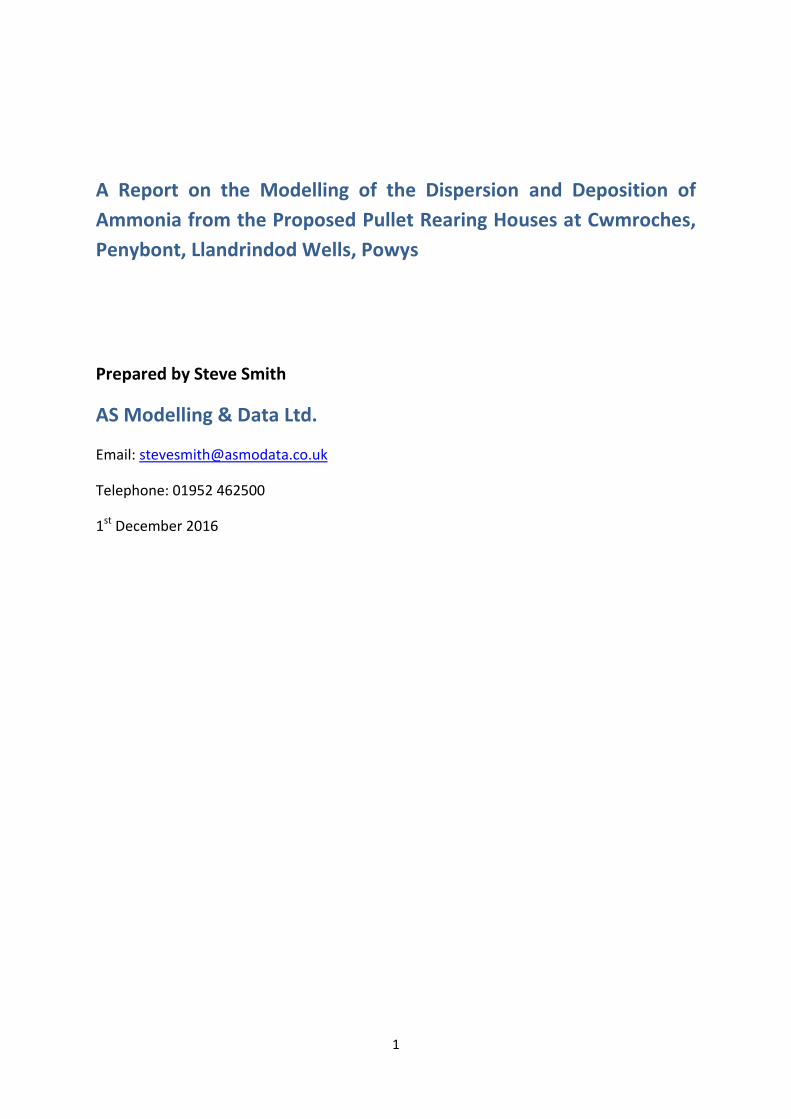
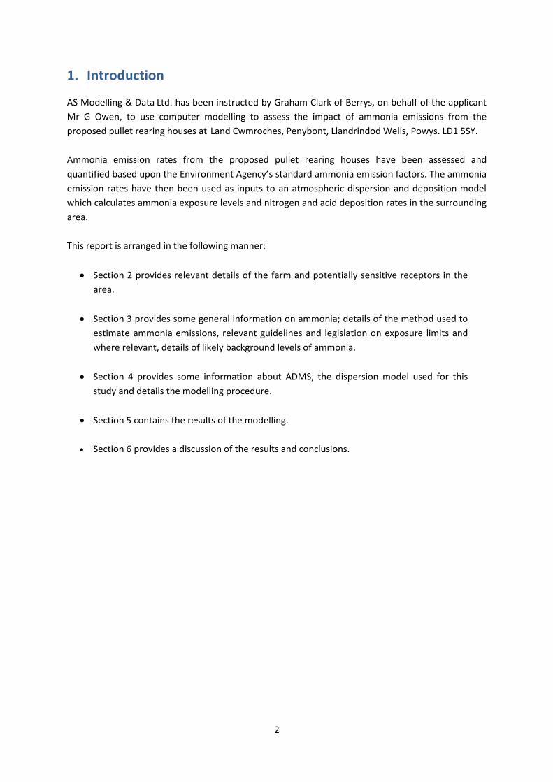
Maps of the surrounding area showing the positions of the poultry unit, the AWs, the SSSIs and the

SAC are provided in Figures 1a and 1b. In these figures; AWs are shaded in olive, SSSIs are shaded in

green, the SAC is shaded in purple and the site of the poultry rearing houses is outlined in blue.

4

Figure 1a. The area surrounding Cwmroches – concentric circles radii 2.0 km (olive), 5.0 km (green) and 10.0 km (purple)

© Crown copyright and database rights. 2016.

5

Figure 1b. The area surrounding Cwmroches – a closer view

© Crown copyright and database rights. 2016.

6

3. Ammonia, Background Levels, Critical Levels & Loads & Emission

Rates

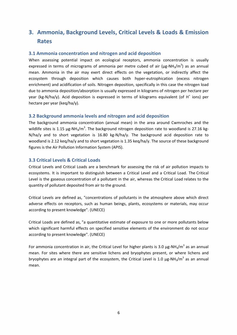
3.1 Ammonia concentration and nitrogen and acid deposition

When assessing potential impact on ecological receptors, ammonia concentration is usually

expressed in terms of micrograms of ammonia per metre cubed of air (µg-NH3/m3) as an annual

mean. Ammonia in the air may exert direct effects on the vegetation, or indirectly affect the

ecosystem through deposition which causes both hyper-eutrophication (excess nitrogen

enrichment) and acidification of soils. Nitrogen deposition, specifically in this case the nitrogen load

due to ammonia deposition/absorption is usually expressed in kilograms of nitrogen per hectare per

year (kg-N/ha/y). Acid deposition is expressed in terms of kilograms equivalent (of H+ ions) per

hectare per year (keq/ha/y).

3.2 Background ammonia levels and nitrogen and acid deposition The background ammonia concentration (annual mean) in the area around Cwmroches and the

wildlife sites is 1.15 µg-NH3/m3. The background nitrogen deposition rate to woodland is 27.16 kg-

N/ha/y and to short vegetation is 16.80 kg-N/ha/y. The background acid deposition rate to

woodland is 2.12 keq/ha/y and to short vegetation is 1.35 keq/ha/y. The source of these background

figures is the Air Pollution Information System (APIS).

3.3 Critical Levels & Critical Loads

Critical Levels and Critical Loads are a benchmark for assessing the risk of air pollution impacts to

ecosystems. It is important to distinguish between a Critical Level and a Critical Load. The Critical

Level is the gaseous concentration of a pollutant in the air, whereas the Critical Load relates to the

quantity of pollutant deposited from air to the ground.

Critical Levels are defined as, "concentrations of pollutants in the atmosphere above which direct

adverse effects on receptors, such as human beings, plants, ecosystems or materials, may occur

according to present knowledge". (UNECE)

Critical Loads are defined as, "a quantitative estimate of exposure to one or more pollutants below

which significant harmful effects on specified sensitive elements of the environment do not occur

according to present knowledge". (UNECE)

For ammonia concentration in air, the Critical Level for higher plants is 3.0 µg-NH3/m3 as an annual

mean. For sites where there are sensitive lichens and bryophytes present, or where lichens and

bryophytes are an integral part of the ecosystem, the Critical Level is 1.0 µg-NH3/m3 as an annual

mean.

7

Critical Loads for nutrient nitrogen are set under the Convention on Long-Range Transboundary Air

Pollution. They are based on empirical evidence, mainly observations from experiments and gradient

studies. Critical Loads are given as ranges (e.g. 10-20 kg-N/ha/y); these ranges reflect variation in

ecosystem response across Europe.

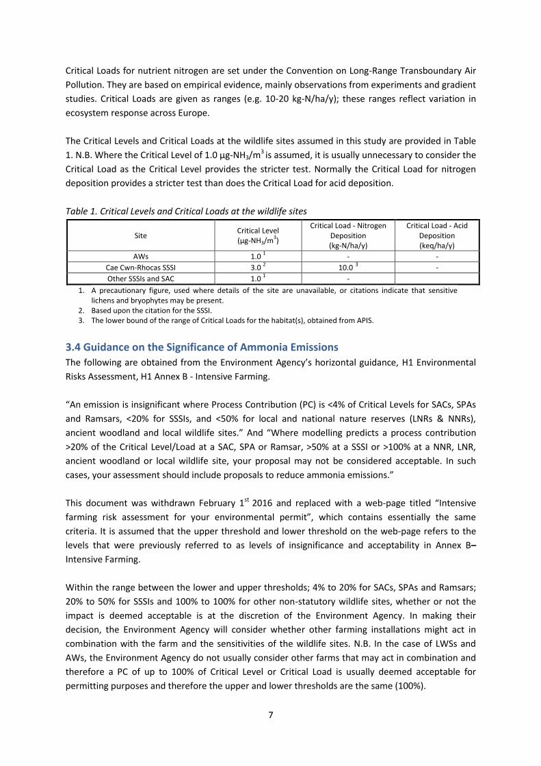
The Critical Levels and Critical Loads at the wildlife sites assumed in this study are provided in Table

1. N.B. Where the Critical Level of 1.0 µg-NH3/m3 is assumed, it is usually unnecessary to consider the

Critical Load as the Critical Level provides the stricter test. Normally the Critical Load for nitrogen

deposition provides a stricter test than does the Critical Load for acid deposition.

Table 1. Critical Levels and Critical Loads at the wildlife sites

Site Critical Level (µg-NH3/m

3)

Critical Load - Nitrogen Deposition (kg-N/ha/y)

Critical Load - Acid Deposition (keq/ha/y)

AWs 1.0 1 -

-

Cae Cwn-Rhocas SSSI 3.0 2 10.0

3 -

Other SSSIs and SAC 1.0 1 -

1. A precautionary figure, used where details of the site are unavailable, or citations indicate that sensitive lichens and bryophytes may be present.

2. Based upon the citation for the SSSI. 3. The lower bound of the range of Critical Loads for the habitat(s), obtained from APIS.

3.4 Guidance on the Significance of Ammonia Emissions

The following are obtained from the Environment Agency’s horizontal guidance, H1 Environmental

Risks Assessment, H1 Annex B - Intensive Farming.

“An emission is insignificant where Process Contribution (PC) is <4% of Critical Levels for SACs, SPAs

and Ramsars, <20% for SSSIs, and <50% for local and national nature reserves (LNRs & NNRs),

ancient woodland and local wildlife sites.” And “Where modelling predicts a process contribution

>20% of the Critical Level/Load at a SAC, SPA or Ramsar, >50% at a SSSI or >100% at a NNR, LNR,

ancient woodland or local wildlife site, your proposal may not be considered acceptable. In such

cases, your assessment should include proposals to reduce ammonia emissions.”

This document was withdrawn February 1st 2016 and replaced with a web-page titled “Intensive

farming risk assessment for your environmental permit”, which contains essentially the same

criteria. It is assumed that the upper threshold and lower threshold on the web-page refers to the

levels that were previously referred to as levels of insignificance and acceptability in Annex B–

Intensive Farming.

Within the range between the lower and upper thresholds; 4% to 20% for SACs, SPAs and Ramsars;

20% to 50% for SSSIs and 100% to 100% for other non-statutory wildlife sites, whether or not the

impact is deemed acceptable is at the discretion of the Environment Agency. In making their

decision, the Environment Agency will consider whether other farming installations might act in

combination with the farm and the sensitivities of the wildlife sites. N.B. In the case of LWSs and

AWs, the Environment Agency do not usually consider other farms that may act in combination and

therefore a PC of up to 100% of Critical Level or Critical Load is usually deemed acceptable for

permitting purposes and therefore the upper and lower thresholds are the same (100%).

8

Note that this guidance is presented as it provides the only published guidance on the significance

and acceptability of ammonia emission from intensive farming. For installation other than permitted

intensive farming, the level of insignificance for a pollutant is generally accepted to be 1% of the

Critical Level or Critical Load and higher levels may be acceptable when considered in-combination

with background levels, if the Critical Level or Critical Load is not exceeded (a total of 70% of Critical

Level or Critical Load is usually considered to be the maximum acceptable level). However, since the

Critical Level or Critical Load for ammonia and nitrogen and acid deposition are, in general, already

exceeded across much of the UK, if this approach were adopted, no process contribution of more

than 1% would be allowed and therefore a more pragmatic approach such as the Environment

Agency’s is required.

3.5 Quantification of Ammonia Emissions

Ammonia emission rates from poultry houses depend on many factors and are likely to be highly

variable. However, the benchmarks for assessing impacts of ammonia and nitrogen deposition are

framed in terms of an annual mean ammonia concentration and annual nitrogen deposition rates.

To obtain relatively robust figures for these statistics, it is not necessary to model short term

temporal variations and a steady continuous emission rate can be assumed. In fact, modelling short

term temporal variations might introduce rather more uncertainty than modelling continuous

emissions.

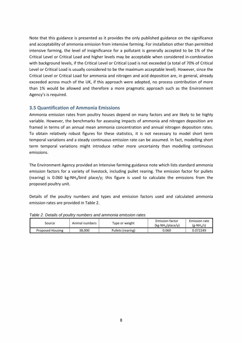
The Environment Agency provided an Intensive farming guidance note which lists standard ammonia

emission factors for a variety of livestock, including pullet rearing. The emission factor for pullets

(rearing) is 0.060 kg-NH3/bird place/y; this figure is used to calculate the emissions from the

proposed poultry unit.

Details of the poultry numbers and types and emission factors used and calculated ammonia

emission rates are provided in Table 2.

Table 2. Details of poultry numbers and ammonia emission rates

Source Animal numbers Type or weight Emission factor

(kg-NH3/place/y) Emission rate

(g-NH3/s)

Proposed Housing 38,000 Pullets (rearing) 0.060 0.072249

9

4. The Atmospheric Dispersion Modelling System (ADMS) and

model parameters

The Atmospheric Dispersion Modelling System (ADMS) ADMS 5 is a new generation Gaussian plume

air dispersion model, which means that the atmospheric boundary layer properties are characterised

by two parameters; the boundary layer depth and the Monin-Obukhov length rather than in terms

of the single parameter Pasquill-Gifford class.

Dispersion under convective meteorological conditions uses a skewed Gaussian concentration

distribution (shown by validation studies to be a better representation than a symmetrical Gaussian

expression).

ADMS has a number of model options including: dry and wet deposition; NOx chemistry; impacts of

hills; variable roughness; buildings and coastlines; puffs; fluctuations; odours; radioactivity decay

(and γ-ray dose); condensed plume visibility; time varying sources and inclusion of background

concentrations.

ADMS has an in-built meteorological pre-processor that allows flexible input of meteorological data

both standard and more specialist. Hourly sequential and statistical data can be processed and all

input and output meteorological variables are written to a file after processing.

The user defines the pollutant, the averaging time (which may be an annual average or a shorter

period), which percentiles and exceedance values to calculate, whether a rolling average is required

or not and the output units. The output options are designed to be flexible to cater for the variety of

air quality limits which can vary from country to country and are subject to revision.

10

4.1 Meteorological data

Computer modelling of dispersion requires hourly sequential meteorological data and to provide

robust statistics the record should be of a suitable length; preferably four years or longer.

The meteorological data used in this study is obtained from assimilation and short term forecast

fields of the Numerical Weather Prediction (NWP) system known as the Global Forecast System

(GFS).

The GFS is a spectral model and data are archived at a horizontal resolution of 0.25 degrees, which is

approximately 25 km over the UK (formerly 0.5 degrees, or approximately 50 km). The GFS

resolution adequately captures major topographical features and the broad-scale characteristics of

the weather over the UK. Smaller scale topological features may be included in the dispersion

modelling by using the flow field module of ADMS (FLOWSTAR). The use of NWP data has

advantages over traditional meteorological records because:

Calm periods in traditional records may be over represented, this is because the

instrumentation used may not record wind speed below approximately 0.5 m/s and start

up wind speeds may be greater than 1.0 m/s. In NWP data, the wind speed is continuous

down to 0.0 m/s, allowing the calms module of ADMS to function correctly.

Traditional records may include very local deviations from the broad-scale wind flow that

would not necessarily be representative of the site being modelled; these deviations are

difficult to identify and remove from a meteorological record. Conversely, local effects at

the site being modelled are relatively easy to impose on the broad-scale flow and

provided horizontal resolution is not too great, the meteorological records from NWP

data may be expected to represent well the broad-scale flow.

Information on the state of the atmosphere above ground level which would otherwise

be estimated by the meteorological pre-processor may be included explicitly.

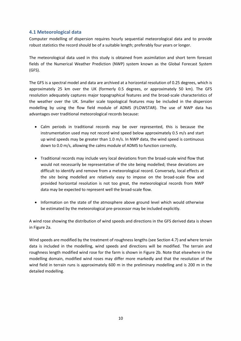
A wind rose showing the distribution of wind speeds and directions in the GFS derived data is shown

in Figure 2a.

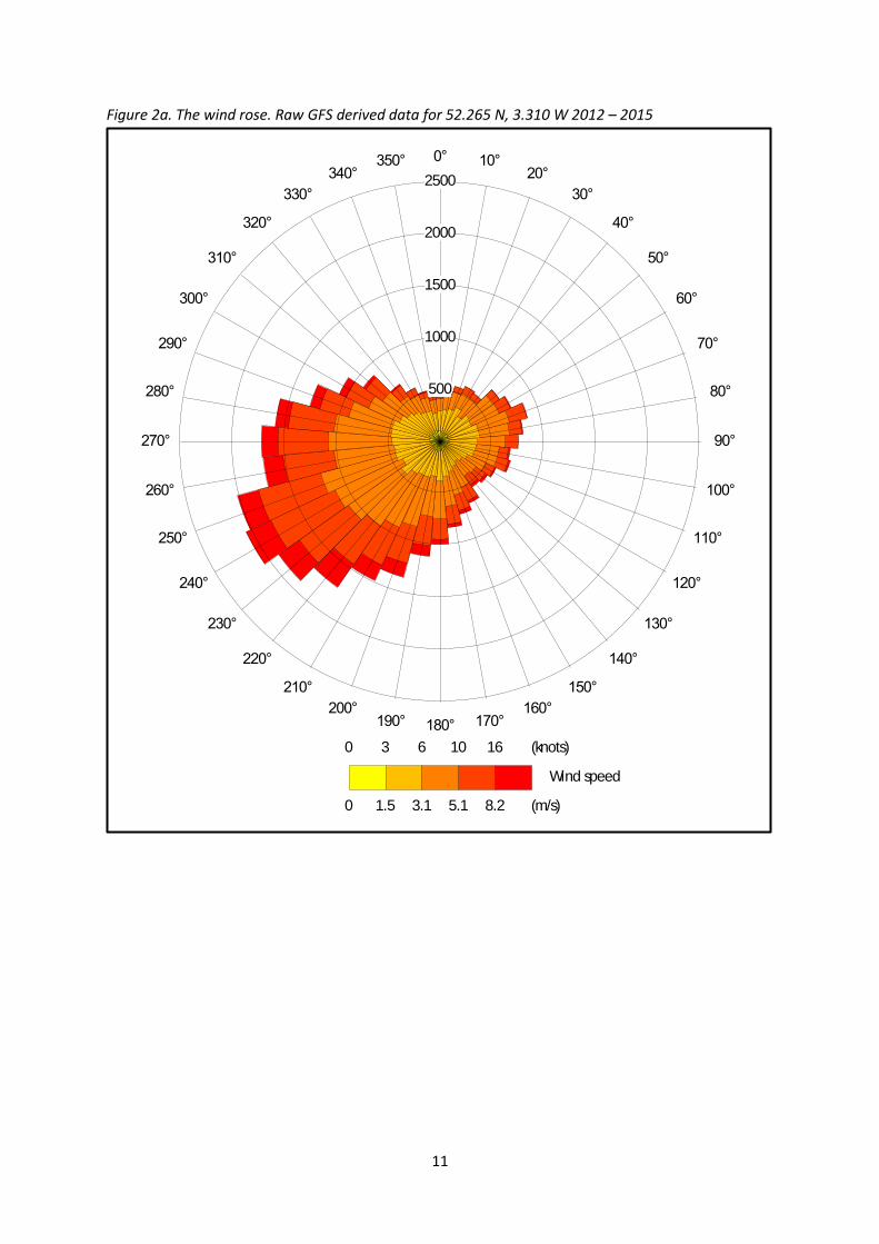
Wind speeds are modified by the treatment of roughness lengths (see Section 4.7) and where terrain

data is included in the modelling, wind speeds and directions will be modified. The terrain and

roughness length modified wind rose for the farm is shown in Figure 2b. Note that elsewhere in the

modelling domain, modified wind roses may differ more markedly and that the resolution of the

wind field in terrain runs is approximately 600 m in the preliminary modelling and is 200 m in the

detailed modelling.

11

Figure 2a. The wind rose. Raw GFS derived data for 52.265 N, 3.310 W 2012 – 2015

\\Octo3\octo3_work\modelling\Cwmroaches\GFS_52.265_-3.31_ADMS_010112_010116.met

0

0

3

1.5

6

3.1

10

5.1

16

8.2

(knots)

(m/s)

Wind speed

0° 10°20°

30°

40°

50°

60°

70°

80°

90°

100°

110°

120°

130°

140°

150°

160°170°180°190°

200°

210°

220°

230°

240°

250°

260°

270°

280°

290°

300°

310°

320°

330°

340°350°

500

1000

1500

2000

2500

12

Figure 2b. The wind rose. FLOWSTAR modified GFS data for the site of the poultry unit (NGR 310600,

263850)

M:\Projects\Cwmroches_Farm\modelling\FLOWSTAR_52.265_-3.31_ADMS_010112_010116.csv

0

0

3

1.5

6

3.1

10

5.1

16

8.2

(knots)

(m/s)

Wind speed

0° 10°20°

30°

40°

50°

60°

70°

80°

90°

100°

110°

120°

130°

140°

150°

160°170°180°190°

200°

210°

220°

230°

240°

250°

260°

270°

280°

290°

300°

310°

320°

330°

340°350°

500

1000

1500

2000

2500

13

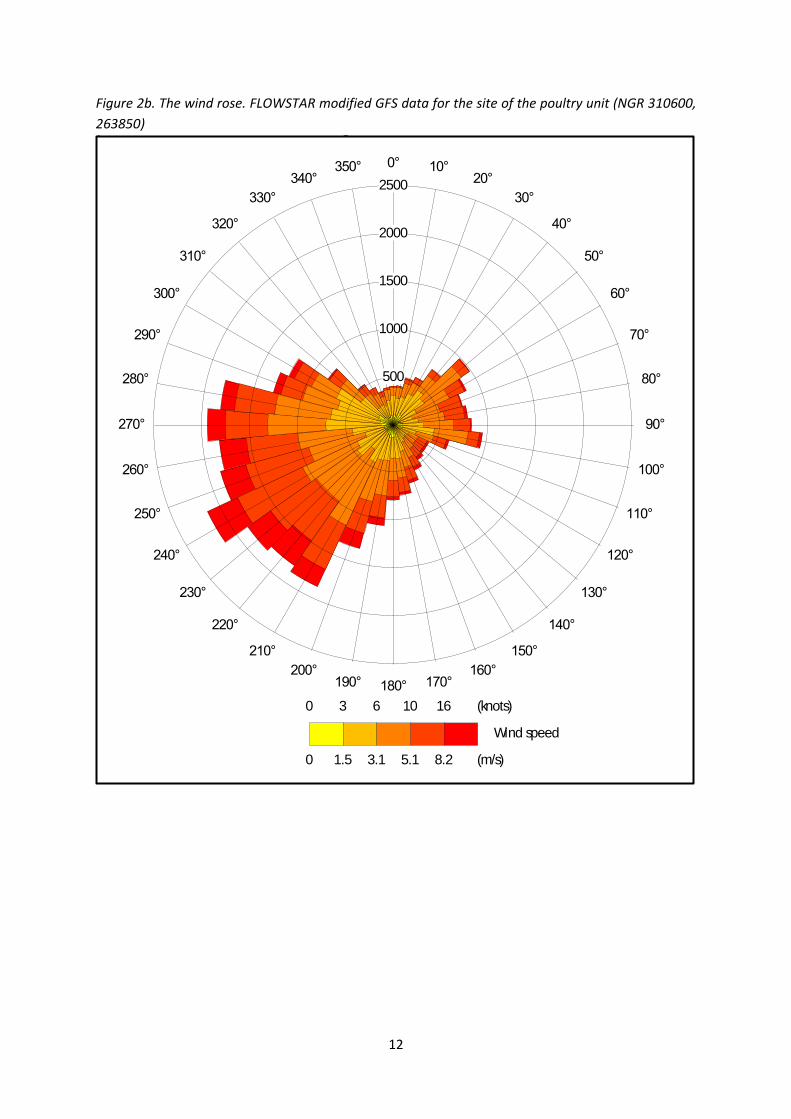
4.2 Emission sources

Emissions from the chimneys of the uncapped high speed ridge mounted fans on the proposed

poultry houses are represented by three point sources per house within ADMS (PR1 a, b & c and PR2

a, b & c). Details of the point source parameters are shown in Table 3. The positions of the point

sources may be seen in Figure 3.

Table 3. Point source parameters

Source ID Height

(m) Diameter

(m)

Efflux velocity

(m/s)

Emission temperature

(˚C)

Emission rate per source

(g-NH3/s)

PR1 a, b & c 6.5 0.8 11.0 21.0 0.010838

PR2 a, b & c 6.5 0.8 11.0 21.0 0.013245

4.3 Modelled buildings

The structure of the poultry houses may affect the plumes from the point sources. Therefore, the

buildings are modelled within ADMS. The positions of the modelled buildings may be seen in Figure

3, where they are marked by grey rectangles.

Figure 3. The positions of modelled buildings & sources

© Crown copyright and database rights. 2016.

14

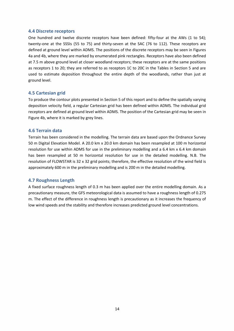
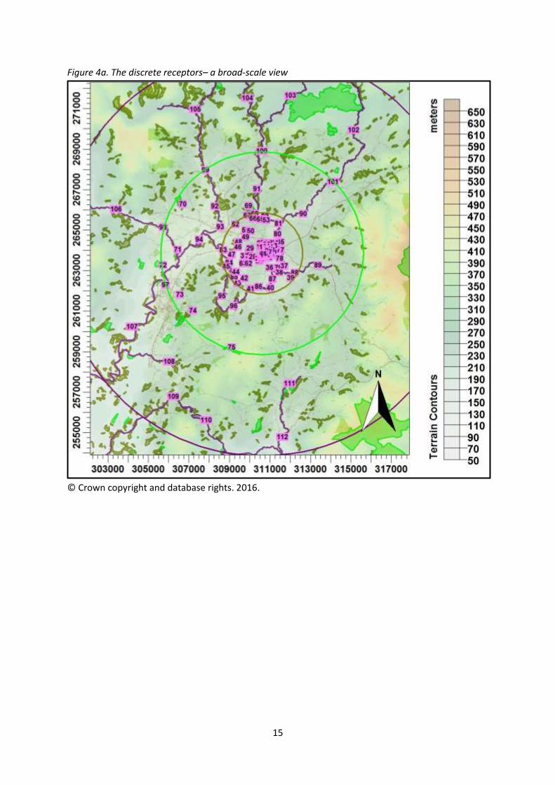
4.4 Discrete receptors

One hundred and twelve discrete receptors have been defined: fifty-four at the AWs (1 to 54);

twenty-one at the SSSIs (55 to 75) and thirty-seven at the SAC (76 to 112). These receptors are

defined at ground level within ADMS. The positions of the discrete receptors may be seen in Figures

4a and 4b, where they are marked by enumerated pink rectangles. Receptors have also been defined

at 7.5 m above ground level at closer woodland receptors; these receptors are at the same positions

as receptors 1 to 20; they are referred to as receptors 1C to 20C in the Tables in Section 5 and are

used to estimate deposition throughout the entire depth of the woodlands, rather than just at

ground level.

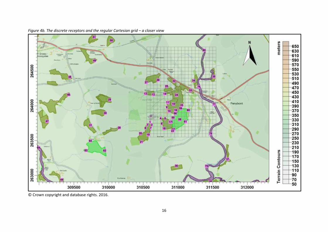
4.5 Cartesian grid

To produce the contour plots presented in Section 5 of this report and to define the spatially varying

deposition velocity field, a regular Cartesian grid has been defined within ADMS. The individual grid

receptors are defined at ground level within ADMS. The position of the Cartesian grid may be seen in

Figure 4b, where it is marked by grey lines.

4.6 Terrain data

Terrain has been considered in the modelling. The terrain data are based upon the Ordnance Survey

50 m Digital Elevation Model. A 20.0 km x 20.0 km domain has been resampled at 100 m horizontal

resolution for use within ADMS for use in the preliminary modelling and a 6.4 km x 6.4 km domain

has been resampled at 50 m horizontal resolution for use in the detailed modelling. N.B. The

resolution of FLOWSTAR is 32 x 32 grid points; therefore, the effective resolution of the wind field is

approximately 600 m in the preliminary modelling and is 200 m in the detailed modelling.

4.7 Roughness Length

A fixed surface roughness length of 0.3 m has been applied over the entire modelling domain. As a

precautionary measure, the GFS meteorological data is assumed to have a roughness length of 0.275

m. The effect of the difference in roughness length is precautionary as it increases the frequency of

low wind speeds and the stability and therefore increases predicted ground level concentrations.

15

Figure 4a. The discrete receptors– a broad-scale view

© Crown copyright and database rights. 2016.

16

Figure 4b. The discrete receptors and the regular Cartesian grid – a closer view

© Crown copyright and database rights. 2016.

17

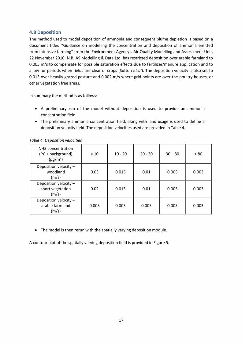
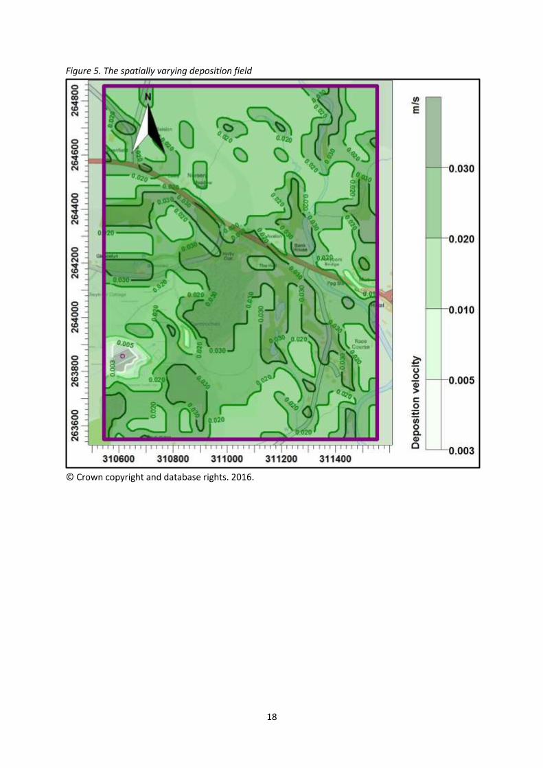
4.8 Deposition

The method used to model deposition of ammonia and consequent plume depletion is based on a

document titled “Guidance on modelling the concentration and deposition of ammonia emitted

from intensive farming” from the Environment Agency’s Air Quality Modelling and Assessment Unit,

22 November 2010. N.B. AS Modelling & Data Ltd. has restricted deposition over arable farmland to

0.005 m/s to compensate for possible saturation effects due to fertilizer/manure application and to

allow for periods when fields are clear of crops (Sutton et al). The deposition velocity is also set to

0.015 over heavily grazed pasture and 0.002 m/s where grid points are over the poultry houses, or

other vegetation free areas.

In summary the method is as follows:

A preliminary run of the model without deposition is used to provide an ammonia

concentration field.

The preliminary ammonia concentration field, along with land usage is used to define a

deposition velocity field. The deposition velocities used are provided in Table 4.

Table 4. Deposition velocities

NH3 concentration (PC + background)

(µg/m3) < 10 10 - 20 20 - 30 30 – 80 > 80

Deposition velocity – woodland

(m/s) 0.03 0.015 0.01 0.005 0.003

Deposition velocity – short vegetation

(m/s) 0.02 0.015 0.01 0.005 0.003

Deposition velocity – arable farmland

(m/s) 0.005 0.005 0.005 0.005 0.003

The model is then rerun with the spatially varying deposition module.

A contour plot of the spatially varying deposition field is provided in Figure 5.

18

Figure 5. The spatially varying deposition field

© Crown copyright and database rights. 2016.

19

5. Details of the Model Runs and Results

5.1 Preliminary modelling

ADMS was run a total of twelve times, once for each year of the meteorological record in three

modes:

In basic mode without calms, or terrain – GFS data.

With calms and without terrain – GFS data.

Without calms and with terrain – GFS data.

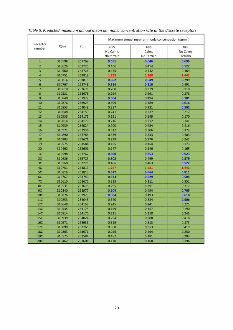
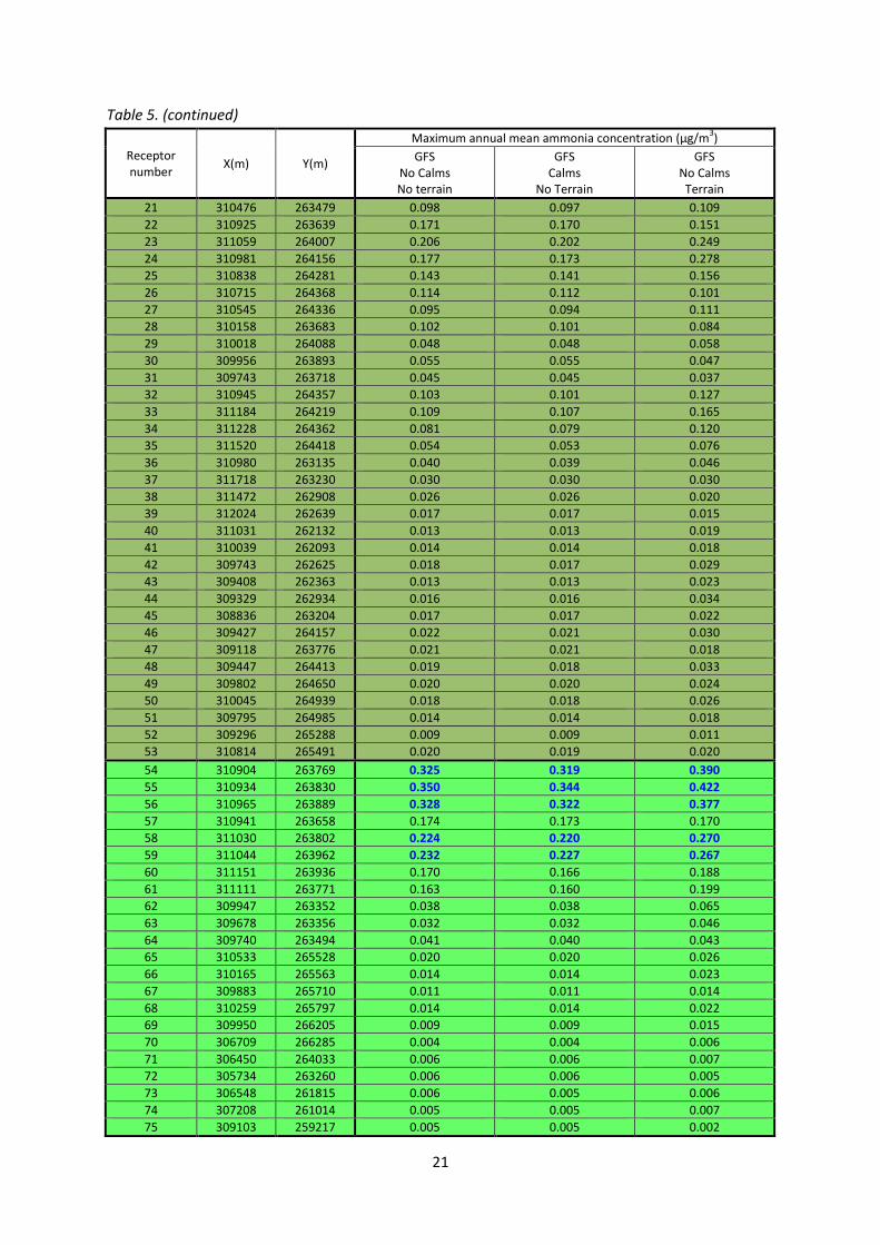
For each mode, statistics for the maximum annual mean ammonia concentration at each receptor

were compiled.

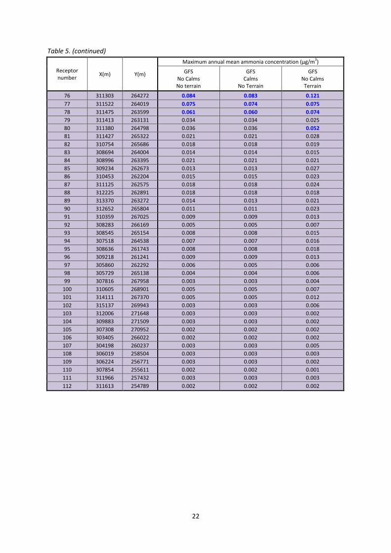
Details of the predicted annual mean ammonia concentrations at each receptor are provided in

Table 5. In the Table, predicted ammonia concentrations that are in excess of the Environment

Agency’s upper threshold (20% of Critical Level or Load for a SAC, 50% of Critical Level or Load for a

SSSI and 100% of Critical Level or Load for an AW) are coloured red. Concentrations in the range

between the Environment Agency’s upper threshold and lower threshold (4% to 20% for a SAC, 20%

to 50% for a SSSI and 50% 1 to 100% for an AW) are coloured blue. For convenience, cells referring to

AWs are shaded olive, cells referring to SSSIs are shaded green and cells referring to the SAC are

shaded purple.

1. The pre-February 2016 value is retained.

20

Table 5. Predicted maximum annual mean ammonia concentration rate at the discrete receptors

Receptor number

X(m) Y(m)

Maximum annual mean ammonia concentration (µg/m3)

GFS No Calms No terrain

GFS Calms

No Terrain

GFS No Calms

Terrain

1 310598 263762 0.651 0.646 0.696

2 310626 263725 0.456 0.454 0.522

3 310560 263726 0.435 0.432 0.464

4 310751 263819 1.225 1.200 1.442

5 310816 263815 0.662 0.649 0.799

6 310767 263743 0.514 0.510 0.491

7 310610 263676 0.280 0.279 0.310

8 310531 263678 0.264 0.261 0.278

9 310840 263977 0.504 0.494 0.701

10 310876 263923 0.499 0.489 0.616

11 310853 264048 0.337 0.331 0.502

12 310648 264159 0.241 0.237 0.217

13 310535 264175 0.151 0.149 0.170

14 310814 264170 0.216 0.212 0.241

15 310939 264024 0.290 0.284 0.416

16 310971 263936 0.312 0.306 0.372

17 310890 263765 0.339 0.333 0.403

18 310803 263671 0.278 0.276 0.242

19 310575 263584 0.155 0.154 0.173

20 310462 263601 0.147 0.146 0.165

1C 310598 263762 0.860 0.853 0.923

2C 310626 263725 0.502 0.499 0.579

3C 310560 263726 0.466 0.463 0.522

4C 310751 263819 1.247 1.221 1.443

5C 310816 263815 0.677 0.664 0.811

6C 310767 263743 0.533 0.529 0.504

7C 310610 263676 0.313 0.311 0.351

8C 310531 263678 0.295 0.291 0.317

9C 310840 263977 0.504 0.494 0.705

10C 310876 263923 0.504 0.493 0.618

11C 310853 264048 0.340 0.334 0.506

12C 310648 264159 0.245 0.241 0.221

13C 310535 264175 0.159 0.157 0.190

14C 310814 264170 0.221 0.218 0.245

15C 310939 264024 0.294 0.288 0.418

16C 310971 263936 0.319 0.313 0.373

17C 310890 263765 0.360 0.353 0.419

18C 310803 263671 0.296 0.294 0.250

19C 310575 263584 0.182 0.181 0.203

20C 310462 263601 0.170 0.168 0.194

21

Table 5. (continued)

Receptor number

X(m) Y(m)

Maximum annual mean ammonia concentration (µg/m3)

GFS No Calms No terrain

GFS Calms

No Terrain

GFS No Calms

Terrain

21 310476 263479 0.098 0.097 0.109

22 310925 263639 0.171 0.170 0.151

23 311059 264007 0.206 0.202 0.249

24 310981 264156 0.177 0.173 0.278

25 310838 264281 0.143 0.141 0.156

26 310715 264368 0.114 0.112 0.101

27 310545 264336 0.095 0.094 0.111

28 310158 263683 0.102 0.101 0.084

29 310018 264088 0.048 0.048 0.058

30 309956 263893 0.055 0.055 0.047

31 309743 263718 0.045 0.045 0.037

32 310945 264357 0.103 0.101 0.127

33 311184 264219 0.109 0.107 0.165

34 311228 264362 0.081 0.079 0.120

35 311520 264418 0.054 0.053 0.076

36 310980 263135 0.040 0.039 0.046

37 311718 263230 0.030 0.030 0.030

38 311472 262908 0.026 0.026 0.020

39 312024 262639 0.017 0.017 0.015

40 311031 262132 0.013 0.013 0.019

41 310039 262093 0.014 0.014 0.018

42 309743 262625 0.018 0.017 0.029

43 309408 262363 0.013 0.013 0.023

44 309329 262934 0.016 0.016 0.034

45 308836 263204 0.017 0.017 0.022

46 309427 264157 0.022 0.021 0.030

47 309118 263776 0.021 0.021 0.018

48 309447 264413 0.019 0.018 0.033

49 309802 264650 0.020 0.020 0.024

50 310045 264939 0.018 0.018 0.026

51 309795 264985 0.014 0.014 0.018

52 309296 265288 0.009 0.009 0.011

53 310814 265491 0.020 0.019 0.020

54 310904 263769 0.325 0.319 0.390

55 310934 263830 0.350 0.344 0.422

56 310965 263889 0.328 0.322 0.377

57 310941 263658 0.174 0.173 0.170

58 311030 263802 0.224 0.220 0.270

59 311044 263962 0.232 0.227 0.267

60 311151 263936 0.170 0.166 0.188

61 311111 263771 0.163 0.160 0.199

62 309947 263352 0.038 0.038 0.065

63 309678 263356 0.032 0.032 0.046

64 309740 263494 0.041 0.040 0.043

65 310533 265528 0.020 0.020 0.026

66 310165 265563 0.014 0.014 0.023

67 309883 265710 0.011 0.011 0.014

68 310259 265797 0.014 0.014 0.022

69 309950 266205 0.009 0.009 0.015

70 306709 266285 0.004 0.004 0.006

71 306450 264033 0.006 0.006 0.007

72 305734 263260 0.006 0.006 0.005

73 306548 261815 0.006 0.005 0.006

74 307208 261014 0.005 0.005 0.007

75 309103 259217 0.005 0.005 0.002

22

Table 5. (continued)

Receptor number

X(m) Y(m)

Maximum annual mean ammonia concentration (µg/m3)

GFS No Calms No terrain

GFS Calms

No Terrain

GFS No Calms

Terrain

76 311303 264272 0.084 0.083 0.121

77 311522 264019 0.075 0.074 0.075

78 311475 263599 0.061 0.060 0.074

79 311413 263131 0.034 0.034 0.025

80 311380 264798 0.036 0.036 0.052

81 311427 265322 0.021 0.021 0.028

82 310754 265686 0.018 0.018 0.019

83 308694 264004 0.014 0.014 0.015

84 308996 263395 0.021 0.021 0.021

85 309234 262673 0.013 0.013 0.027

86 310453 262204 0.015 0.015 0.023

87 311125 262575 0.018 0.018 0.024

88 312225 262891 0.018 0.018 0.018

89 313370 263272 0.014 0.013 0.021

90 312652 265804 0.011 0.011 0.023

91 310359 267025 0.009 0.009 0.013

92 308283 266169 0.005 0.005 0.007

93 308545 265154 0.008 0.008 0.015

94 307518 264538 0.007 0.007 0.016

95 308636 261743 0.008 0.008 0.018

96 309218 261241 0.009 0.009 0.013

97 305860 262292 0.006 0.005 0.006

98 305729 265138 0.004 0.004 0.006

99 307816 267958 0.003 0.003 0.004

100 310605 268901 0.005 0.005 0.007

101 314111 267370 0.005 0.005 0.012

102 315137 269943 0.003 0.003 0.006

103 312006 271648 0.003 0.003 0.002

104 309883 271509 0.003 0.003 0.002

105 307308 270952 0.002 0.002 0.002

106 303405 266022 0.002 0.002 0.002

107 304198 260237 0.003 0.003 0.005

108 306019 258504 0.003 0.003 0.003

109 306224 256771 0.003 0.003 0.002

110 307854 255611 0.002 0.002 0.001

111 311966 257432 0.003 0.003 0.003

112 311613 254789 0.002 0.002 0.002

23

5.2 Detailed deposition modelling

The detailed deposition modelling was carried out over a domain covering the poultry unit, closer

AWs, Cae Cwn-Rhocas SSSI and closer parts of the River Ithon SAC, where the preliminary modelling

indicated that annual mean ammonia concentrations could potentially exceed the lower threshold

percentage of the relevant Critical Level/Critical Load (4% for the SAC, 20% for the SSSI and 50% for

the AWs). At all other receptors, annual mean ammonia concentrations were predicted to be at

levels below the Environment Agency’s lower threshold percentage of Critical Level/Load for the

site.

Spatially varying deposition and terrain cannot be modelled in conjunction with the calms module of

ADMS. In this case, the preliminary modelling suggests that, with ventilation using elevated high

speed fans, the effect of calms is insignificant. The model was run four times, once for each year of

the meteorological record.

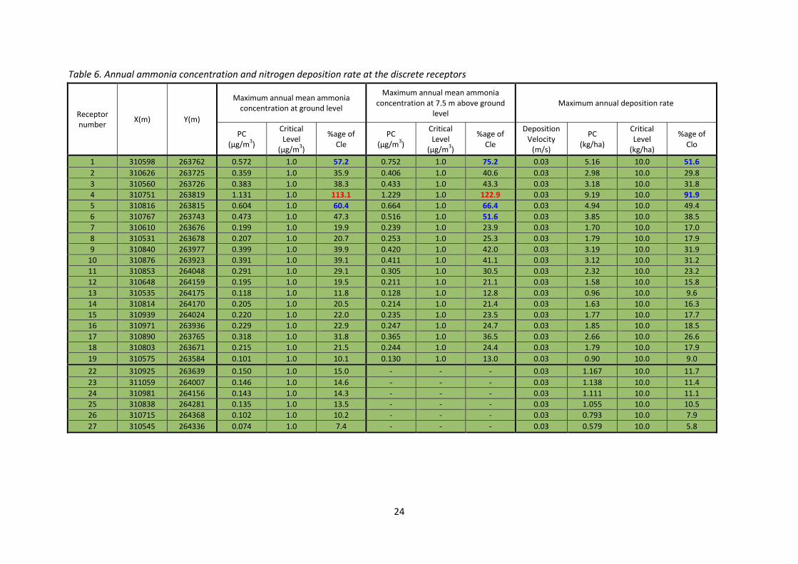
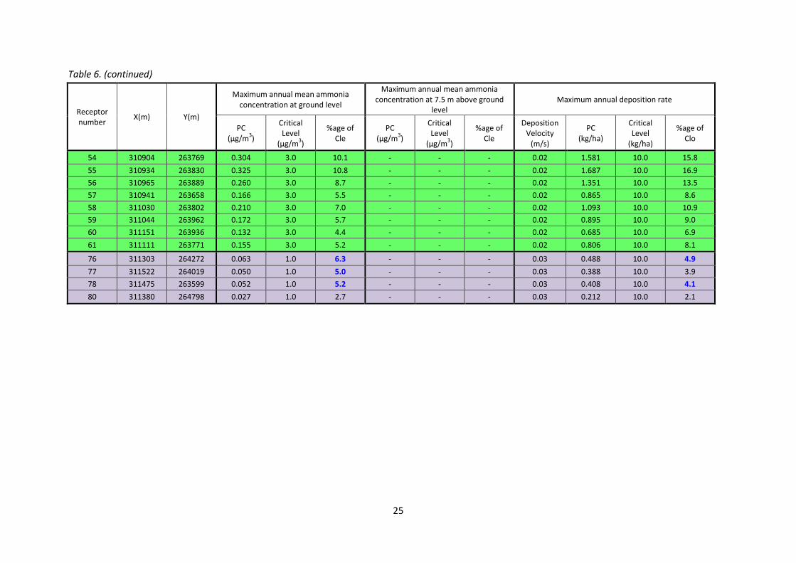
The results of the predicted annual mean ground level ammonia concentrations and annual nitrogen

deposition rates at the discrete receptors within the restricted modelling domain are shown in Table

6. In the Table, predicted ammonia concentrations that are in excess of the Environment Agency’s

upper threshold (20% of Critical Level or Load for a SAC, 50% of Critical Level or Load for a SSSI and

100% of Critical Level or Load for an AW) are coloured red. Concentrations in the range between the

Environment Agency’s upper threshold and lower threshold (4% to 20% for a SAC, 20% to 50% for a

SSSI and 50% 1 to 100% for an AW) are coloured blue. For convenience, cells referring to AWs are

shaded olive, cells referring to SSSIs are shaded green and cells referring to the SAC are shaded

purple. The abbreviations PC, Cle and Clo, used in the tables means Process Contribution, Critical

Level and Critical Load, respectively.

Where receptors at both ground level and 7.5 m are defined, the nitrogen deposition rate is

calculated assuming that 50% of deposition occurs near ground level and 50% at canopy level.

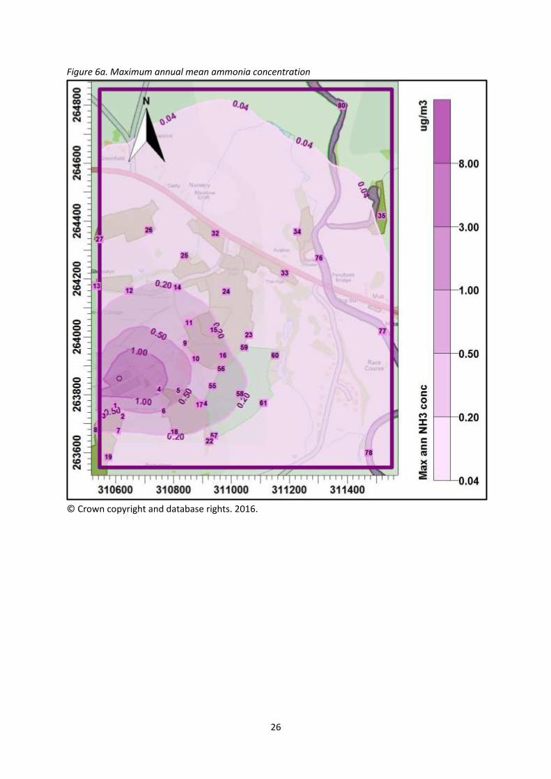
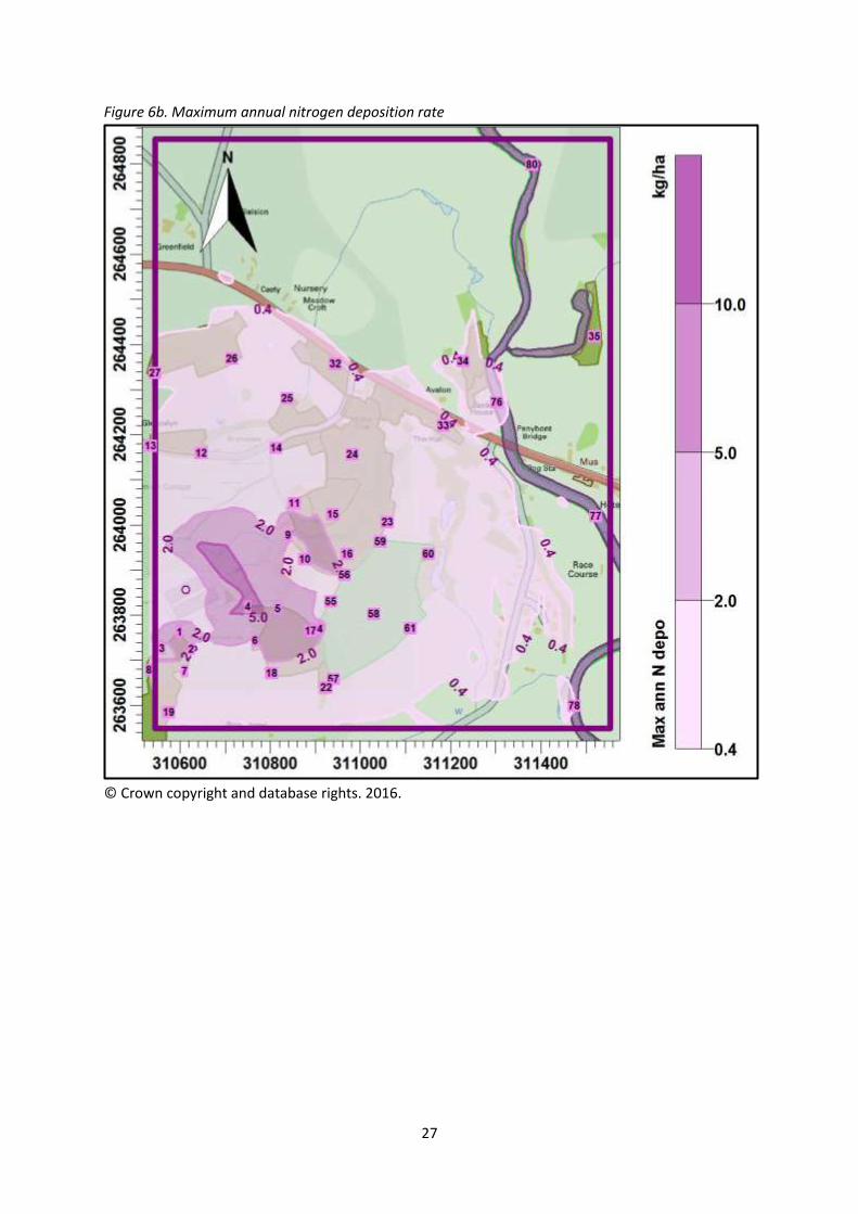
Contour plots of the predicted maximum annual ammonia concentrations and nitrogen deposition

rates are shown in Figures 6a and 6b.

24

Table 6. Annual ammonia concentration and nitrogen deposition rate at the discrete receptors

Receptor number

X(m) Y(m)

Maximum annual mean ammonia concentration at ground level

Maximum annual mean ammonia concentration at 7.5 m above ground

level Maximum annual deposition rate

PC (µg/m

3)

Critical Level

(µg/m3)

%age of Cle

PC (µg/m

3)

Critical Level

(µg/m3)

%age of Cle

Deposition Velocity

(m/s)

PC (kg/ha)

Critical Level

(kg/ha)

%age of Clo

1 310598 263762 0.572 1.0 57.2 0.752 1.0 75.2 0.03 5.16 10.0 51.6

2 310626 263725 0.359 1.0 35.9 0.406 1.0 40.6 0.03 2.98 10.0 29.8

3 310560 263726 0.383 1.0 38.3 0.433 1.0 43.3 0.03 3.18 10.0 31.8

4 310751 263819 1.131 1.0 113.1 1.229 1.0 122.9 0.03 9.19 10.0 91.9

5 310816 263815 0.604 1.0 60.4 0.664 1.0 66.4 0.03 4.94 10.0 49.4

6 310767 263743 0.473 1.0 47.3 0.516 1.0 51.6 0.03 3.85 10.0 38.5

7 310610 263676 0.199 1.0 19.9 0.239 1.0 23.9 0.03 1.70 10.0 17.0

8 310531 263678 0.207 1.0 20.7 0.253 1.0 25.3 0.03 1.79 10.0 17.9

9 310840 263977 0.399 1.0 39.9 0.420 1.0 42.0 0.03 3.19 10.0 31.9

10 310876 263923 0.391 1.0 39.1 0.411 1.0 41.1 0.03 3.12 10.0 31.2

11 310853 264048 0.291 1.0 29.1 0.305 1.0 30.5 0.03 2.32 10.0 23.2

12 310648 264159 0.195 1.0 19.5 0.211 1.0 21.1 0.03 1.58 10.0 15.8

13 310535 264175 0.118 1.0 11.8 0.128 1.0 12.8 0.03 0.96 10.0 9.6

14 310814 264170 0.205 1.0 20.5 0.214 1.0 21.4 0.03 1.63 10.0 16.3

15 310939 264024 0.220 1.0 22.0 0.235 1.0 23.5 0.03 1.77 10.0 17.7

16 310971 263936 0.229 1.0 22.9 0.247 1.0 24.7 0.03 1.85 10.0 18.5

17 310890 263765 0.318 1.0 31.8 0.365 1.0 36.5 0.03 2.66 10.0 26.6

18 310803 263671 0.215 1.0 21.5 0.244 1.0 24.4 0.03 1.79 10.0 17.9

19 310575 263584 0.101 1.0 10.1 0.130 1.0 13.0 0.03 0.90 10.0 9.0

22 310925 263639 0.150 1.0 15.0 - - - 0.03 1.167 10.0 11.7

23 311059 264007 0.146 1.0 14.6 - - - 0.03 1.138 10.0 11.4

24 310981 264156 0.143 1.0 14.3 - - - 0.03 1.111 10.0 11.1

25 310838 264281 0.135 1.0 13.5 - - - 0.03 1.055 10.0 10.5

26 310715 264368 0.102 1.0 10.2 - - - 0.03 0.793 10.0 7.9

27 310545 264336 0.074 1.0 7.4 - - - 0.03 0.579 10.0 5.8

25

Table 6. (continued)

Receptor number

X(m) Y(m)

Maximum annual mean ammonia concentration at ground level

Maximum annual mean ammonia concentration at 7.5 m above ground

level Maximum annual deposition rate

PC (µg/m

3)

Critical Level

(µg/m3)

%age of Cle

PC (µg/m

3)

Critical Level

(µg/m3)

%age of Cle

Deposition Velocity

(m/s)

PC (kg/ha)

Critical Level

(kg/ha)

%age of Clo

54 310904 263769 0.304 3.0 10.1 - - - 0.02 1.581 10.0 15.8

55 310934 263830 0.325 3.0 10.8 - - - 0.02 1.687 10.0 16.9

56 310965 263889 0.260 3.0 8.7 - - - 0.02 1.351 10.0 13.5

57 310941 263658 0.166 3.0 5.5 - - - 0.02 0.865 10.0 8.6

58 311030 263802 0.210 3.0 7.0 - - - 0.02 1.093 10.0 10.9

59 311044 263962 0.172 3.0 5.7 - - - 0.02 0.895 10.0 9.0

60 311151 263936 0.132 3.0 4.4 - - - 0.02 0.685 10.0 6.9

61 311111 263771 0.155 3.0 5.2 - - - 0.02 0.806 10.0 8.1

76 311303 264272 0.063 1.0 6.3 - - - 0.03 0.488 10.0 4.9

77 311522 264019 0.050 1.0 5.0 - - - 0.03 0.388 10.0 3.9

78 311475 263599 0.052 1.0 5.2 - - - 0.03 0.408 10.0 4.1

80 311380 264798 0.027 1.0 2.7 - - - 0.03 0.212 10.0 2.1

26

Figure 6a. Maximum annual mean ammonia concentration

© Crown copyright and database rights. 2016.

27

Figure 6b. Maximum annual nitrogen deposition rate

© Crown copyright and database rights. 2016.

28

6. Summary and Conclusions

AS Modelling & Data Ltd. has been instructed by Graham Clark of Berrys, on behalf of the applicant

Mr G Owen, to use computer modelling to assess the impact of ammonia emissions from the

proposed pullet rearing houses at Land Cwmroches, Penybont, Llandrindod Wells, Powys. LD1 5SY.

Ammonia emission rates from the proposed pullet rearing houses have been assessed and

quantified based upon the Environment Agency’s standard ammonia emission factors. The ammonia

emission rates have then been used as inputs to an atmospheric dispersion and deposition model

which calculates ammonia exposure levels and nitrogen and acid deposition rates in the surrounding

area.

There is a predicted exceedance of 100% of the precautionary Critical Level of 1.0 µg-NH3/m3 over

the northernmost tip of the unnamed AW to the south-east of the site of the proposed poultry

houses; this exceedance covers approximately 0.1 ha of the woodland.

At other nearby AWs, the process contributions to the annual mean ammonia concentration and

nitrogen deposition rate are predicted to be below the Environment Agency’s lower threshold

percentage of Critical Level or Critical Load for AWs (100%).

At Cae Cwn-Rhocas SSSI and other SSSIs, the process contributions to the annual mean ammonia

concentration and nitrogen deposition rate are predicted to be below the Environment Agency’s

lower threshold percentage of Critical Level or Critical Load for SSSIs.

At the River Wye SAC, there is a small predicted exceedance of 4% of the precautionary Critical Level

of 1.0 µg-NH3/m3, this exceedance extends along approximately 1.5 km of the SAC to the east of the

site of the proposed poultry houses. There are also small predicted exceedance of 4% of the Critical

Load of 10.0 kg/ha/y, near receptors 76 and 78. It should be noted that the SAC is designated

primarily for aquatic species and that plant species that are sensitive to ammonia (and nitrogen

deposition) are unlikely to be present along this stretch of the river, therefore the higher Critical

Level of 3.0 µg-NH3/m3 may be appropriate, in which case there would be no exceedance of 4% of

the Critical Level. It should also be noted that the Critical Load used for the assessment is the lower

bound of the range of Critical Loads for a habitats such as the banks of the river.

The process contributions to the annual mean ammonia concentration and nitrogen deposition rate

are predicted to be below the Environment Agency’s lower threshold percentage of Critical Level or

Critical Load for SACs (4%) at all other parts of the SAC.

Where exceedances of the lower threshold for non-statutory sites are predicted, some form of

mitigation is usually required. AS Modelling & Data Ltd. would recommend that, if available, to

compensate for possible detrimental effects on the nearby AWs, the woodland is actively managed

for wildlife, and/or, that land of at least a similar area to the exceedance of 100% of the Critical Level

(approximately 0.1 ha) is set aside for nature conservation and be planted/seeded with native

species.

29

Woodland planting schemes, or restoration to traditional unimproved grassland, could replace what

is currently improved grassland with low ecological value. If planted between the poultry unit and

the AWs, the newly planted woodland would act as a sink for ammonia from the poultry houses (and

from other sources of ammonia), thus reducing ammonia concentrations (and nitrogen and acid

deposition rates) at nearby AWs and other sites. Such schemes may be particularly effective at

increasing bio-diversity if they border, or connect with, existing remnants of woodland, or

unimproved grasslands.

30

7. References

Cambridge Environmental Research Consultants (CERC) (website). http://www.cerc.co.uk/environmental-software/ADMS-model.html

Environment Agency H1 Risk Assessment (website). https://www.gov.uk/government/collections/horizontal-guidance-environmental-permitting

M. A. Sutton et al. Measurement and modelling of ammonia exchange over arable croplands. https://enviro.doe.gov.my/lib/digital/1386301476-1-s2.0-S0166111606802748-main.pdf

Misselbrook. et al. Inventory of Ammonia Emissions from UK Agriculture 2011 http://uk-air.defra.gov.uk/assets/documents/reports/cat07/1211291427_nh3inv2011_261112_FINAL_corrected.pdf

United Nations Economic Commission for Europe (UNECE) (website). http://www.unece.org/env/lrtap/WorkingGroups/wge/definitions.htm

UK Air Pollution Information System (APIS) (website). http://www.apis.ac.uk/