A reversal coarsegrained analysis with application to an ...wrap.warwick.ac.uk/57406/1/WRAP_Feng_brb3173.pdf · analysis with application to an altered functional circuit in depression

http://wrap.warwick.ac.uk

Original citation: Guo, Shuixia, Yu, Yun, Zhang, Jie and Feng, Jianfeng. (2013) A reversal coarse-grained analysis with application to an altered functional circuit in depression. Brain and Behavior, Volume 3 (Number 6). pp. 637-648. ISSN 2162-3279 Permanent WRAP url: http://wrap.warwick.ac.uk/57406 Copyright and reuse: The Warwick Research Archive Portal (WRAP) makes this work of researchers of the University of Warwick available open access under the following conditions. This article is made available under the Creative Commons Attribution 3.0 (CC BY 3.0) license and may be reused according to the conditions of the license. For more details see: http://creativecommons.org/licenses/by/3.0/ A note on versions: The version presented in WRAP is the published version, or, version of record, and may be cited as it appears here. For more information, please contact the WRAP Team at: [email protected]

http://wrap.warwick.ac.uk/

http://wrap.warwick.ac.uk/57406

http://creativecommons.org/licenses/by/3.0/

mailto:[email protected]

A reversal coarse-grained analysis with application to analtered functional circuit in depressionShuixia Guo1, Yun Yu1, Jie Zhang2 & Jianfeng Feng2,3

1College of Mathematics and Computer Science, Key Laboratory of High Performance Computing and Stochastic Information Processing

(Ministry of Education of China), Hunan Normal University, Changsha, Hunan, China2Centre for Computational Systems Biology, School of Mathematical Sciences, Fudan University, Shanghai, China3Department of Computer Science, University of Warwick, Coventry, U.K.

Keywords

Reversal coarse-grained analysis, source

location, voxel-wise time series

Correspondence

Jianfeng Feng, Department of Computer

Science, University of Warwick,

Coventry, U.K.

Tel: +44 7799572480; Fax: +44 2476523193;

E-mail: [email protected]

Funding Information

J. F. F is a Royal Society Wolfson Research

Merit Award holder, partially supported by

National Centre for Mathematics and

Interdisciplinary Sciences (NCMIS) of the

Chinese Academy of Sciences and Key

Program of National Natural Science

Foundation of China (No. 91230201). S. X. G.

is supported by the National Natural Science

Foundation of China (NSFC) grant:

11271121, Program for New Century

Excellent Talents in University (NCET) grant,

Key Laboratory of Computational and

Stochastic Mathematics and Its Application

of Hunan province (11K038) and the

Construct Program of the Key Discipline in

Hunan Province. J. Z. is supported by grants

from the Natural Scientific Foundation of

China (61104143 and 61004104).

Received: 14 July 2012; Revised: 9 August

2013; Accepted: 14 August 2013

Brain and Behavior 2013; 3(6): 637–648

doi: 10.1002/brb3.173

Abstract

Introduction: When studying brain function using functional magnetic reso-

nance imaging (fMRI) data containing tens of thousands of voxels, a coarse-

grained approach – dividing the whole brain into regions of interest – is

applied frequently to investigate the organization of the functional network on

a relatively coarse scale. However, a coarse-grained scheme may average out the

fine details over small spatial scales, thus rendering it difficult to identify the

exact locations of functional abnormalities. Methods: A novel and general

approach to reverse the coarse-grained approach by locating the exact sources

of the functional abnormalities is proposed. Results: Thirty-nine patients with

major depressive disorder (MDD) and 37 matched healthy controls are studied.

A circuit comprising the left superior frontal gyrus (SFGdor), right insula

(INS), and right putamen (PUT) exhibit the greatest changes between the

patients with MDD and controls. A reversal coarse-grained analysis is applied

to this circuit to determine the exact location of functional abnormalities.

Conclusions: The voxel-wise time series extracted from the reversal coarse-

grained analysis (source) had several advantages over the original coarse-grained

approach: (1) presence of a larger and detectable amplitude of fluctuations,

which indicates that neuronal activities in the source are more synchronized;

(2) identification of more significant differences between patients and controls

in terms of the functional connectivity associated with the sources; and

(3) marked improvement in performing discrimination tasks. A software pack-

age for pattern classification between controls and patients is available in

Supporting Information.

Introduction

The human brain is a complex system with dynamic

interactions among various brain regions that operate in

a large-scale network. Functional magnetic resonance

imaging (fMRI), which has been applied widely in under-

standing the interworking of the brain, has provided

an unprecedented opportunity to study various brain

disorders, such as depression, Alzheimer’s disease, and

schizophrenia, and may represent the key to the early

ª 2013 The Authors. Brain and Behavior published by Wiley Periodicals, Inc. This is an open access article under the terms of

the Creative Commons Attribution License, which permits use, distribution and reproduction in any medium,

provided the original work is properly cited.

637

diagnosis of such diseases. When studying the brain using

fMRI data, a coarse-grained analysis – dividing the whole

brain into regions of interest (ROIs) – is often adopted to

investigate the functional connectivity (Ogawa et al. 1990,

1992; Humphreys et al. 2007; Kriegeskorte et al. 2010;

Guo et al. 2012) between spatially distributed areas. In

this approach, an ROI-wise time series for each region is

obtained by simply averaging the time series of all voxels

within a specific, coarse brain region (Bassett et al. 2009;

Bullmore and Sporns 2009; Dosenbach et al. 2010).

Useful information contained in relatively fine compo-

nents of the brain may be missed using this approach.

This is because spatial averaging may blur fine patterns

that display significant differences across patient and con-

trol groups. A fine-grained approach – dividing the brain

into smaller areas – may encounter a technical barrier,

that is, very little aberrant functional connectivities can

pass a stringent multicomparison correction. Therefore, it

is crucial to perform a reversal coarse-grained analysis to

obtain more accurate in loci and, therefore, more biologi-

cally precise results.

In our previous paper (Tao et al. 2011), a coarse-

grained analysis was carried out in 39 patients with major

depressive disorder (MDD) and 37 matched controls to

investigate the changes in functional connectivity of

patients with MDD during a task-free (resting-state) para-

digm. A hate circuit comprising the left superior frontal

gyrus (SFGdor), right insula (INS), and right putamen

(PUT) exhibited the greatest changes between the patients

and controls and the changes in these three regions

related to the hate circuit have also been reported in the

literatures (Husain et al. 1991; Strakowski et al. 1999,

2002; Kimbrell et al. 2002; Anand et al. 2005; Kempton

et al. 2011).

Although these three regions exhibited highest signifi-

cant changes in patients with MDD than in controls, they

were too large (from an anatomical point of view) to pro-

vide detailed, clinically relevant information. Coarse brain

regions obtained from different template such as auto-

mated anatomical labeling (AAL) template (Tzourio-

Mazoyer et al. 2002) may contain thousands of voxels,

and different parts of the same region may have different

functions. Locating a relatively fine subregion showing

the greatest change should facilitate the analysis of essen-

tial differences between patients with MDD and controls

and provide more information for clinicians, thereby

helping in decision making in their clinical practice.

In the current paper, we proposed a novel and general

approach to reverse the coarse-grained approach and to

determine the exact location of functional abnormalities.

We applied this approach to the hate circuit. The

intensity of each voxel was used to locate the subregions

of the three structures and to extract voxel-wise time ser-

ies by averaging the time series of the source voxels

located within each region. Our results demonstrated that

the voxel-wise time series extracted from the reversal

coarse-grained analysis have several advantages: (1) a lar-

ger amplitude of fluctuations that are indicative of more

synchronized BOLD signals, (2) more significant differ-

ences between patients and controls in functional connec-

tivity links, and (3) a greater effect on connectivity and a

better performance regarding discrimination accuracy.

Methods

Subjects

Thirty-nine MDD patients (23 females, 16 males; mean

age 27.99 � 7.49 years old; mean education

12.00 � 3.58 years) were recruited from the in- or

outpatient department of the Second Xiangya Hospital of

Central South University in Changsha, Hunan province,

China. The mean illness duration for MDD patients was

27.27 � 37.82 months, and the mean score on the 17

items version of Hamilton rating scale for depression

(HAMD) was 24.97 � 4.99. Thirty-seven normal controls

(14 females, 23 males; mean age 28.22 � 6.47 years old;

mean education 13.32 � 3.29 years) were also recruited.

The two groups have no significant difference in sex

(chi-square test, P > 0.05), age analyses of variance

(ANOVA, P > 0.05), and education (two samples t-test,

P > 0.05). The detailed demographics of these two groups

are shown in Table 1.

All patients met the following inclusion criteria:

(1) Current MDD attack as assessed by two experienced

psychiatrists using the Structural Clinical Interview for

Diagnostic and Statistical Manual of Mental Disorders

(DSM-IV); (2) 18–45 years of age; (3) right-handed Han

Chinese; (4) HAMD scores of at least 17.

Patients and healthy controls were excluded if they

had any of the following: (1) a history of neurological

diseases or other serious physical diseases; (2) a history

of electroconvulsive therapy; (3) history of substance

abuse (i.e., drugs, alcohol, and other psychoactive sub-

stance); (4) any contraindications for MRI. This study

Table 1. Subject demographics.

Depression

patients n = 39

Controls

n = 37 P-value

Age (year) 27.99 � 7.7 28.22 � 6.47 0.964

Education (year) 12.00 � 3.58 13.32 � 3.29 0.306

Sex (M/F) 23/16 14/23 0.087

Illness duration

(year)

2.42 � 3.26 n.a. n.a.

HAMD 24.97 � 5.07 n.a. n.a.

638 ª 2013 The Authors. Brain and Behavior published by Wiley Periodicals, Inc.

A reversal Coarse-Grained Analysis S. Guo et al.

was approved by the Ethics Committee of the Second

Xiangya Hospital, Central South University, Hunan,

China. Written informed consent was obtained from all

subjects.

Imaging acquisitions and datapreprocessing

All image data were acquired using a 1.5T Siemens GE

Signa Twinspeed Scanner (General Electric Medical

System, Milwaukee, WI). The resting-state fMRI was

performed with a gradient-echo echo planar sequence. Sub-

jects were asked to relax and think of nothing in particular

with eyes closed but were requested not to fall asleep. A

total of 180 volumes of echo-planar imagings were

obtained axially (repetition time, 2000 msec; echo time,

40 msec; slices, 20; thickness, 5 mm; gap, 1 mm; field of

view (FOV), 24′24 cm2; resolution, 64′64; flip angle, 90

degrees).

Prior to preprocessing, the first 10 volumes were dis-

carded to allow for scanner stabilization and the subjects’

adaptation to the environment. fMRI data preprocessing

was then conducted by SPM8 (http://www.fil.ion.ucl.ac.

uk/spm) and a data processing assistant for resting-state

fMRI (DPARSF) (Yan and Zang 2010). Briefly, the

remaining functional scans were first corrected for

within-scan acquisition time differences between slices,

and then realigned to the middle volume to correct for

interscan head motions. Subsequently, the functional

scans were spatially normalized by using T1 image unified

segmentation (done by DPARSF directly) and resampled

to 3 9 393 mm3. After normalization, the BOLD signal

of each voxel was first detrended to abandon a linear

trend and then passed through a band-pass filter

(0.01–0.08 Hz) to reduce low-frequency drift and high-

frequency physiological noise. Finally, nuisance covariates

including head motion parameters, global mean signals,

white matter signals, and cerebrospinal signals were

regressed out from the BOLD signals. The masks of three

ROIs related to the hate circuit (left SFGdor, right INS,

and right PUT) were generated using the free software

WFU_PickAtlas (http://www.ansir.wfubmc.edu) (Maldjian

et al. 2003). Time series of each voxel within three ROIs

were extracted. There were 1184, 597, and 352 voxels,

respectively, in these three ROIs.

Source location

In our previous paper, a coarse-grained analysis, which

is conducted by dividing the whole brain into 90 AAL

ROIs was performed to investigate the significant

changes between patients with MDD and matched con-

trols. A so-called hate circuit composing of left SFGdor,

right INS, and right PUT exhibited the greatest changes.

Here, a reversal coarse-grained analysis, conducted by

dividing the whole brain into voxels, was carried out to

these three regions to find out the essential difference

between these two groups. First of all, the Pearson cor-

relation coefficient of all interregional links (for voxels)

are calculated between SFGdor versus INS and INS

versus PUT, a fisher’s r-to-z transformation is utilized to

convert each correlation coefficient rij into Zij to

improve the normality. After that, a two-sample t-test

was then performed for all interregional links. A signifi-

cance level of P < 0.05 was used to find out the

dysfunctional links. As pointed in Zhang et al. (2012),

the functional connectivity between two voxels is very

sensitive to noise which is ineluctable even after filtering,

the located source regions are not usually robust. To

circumvent this problem, for each selected voxel i in

region A, a dysfunction intensity for this voxel is

defined as following:

intensityðiÞ ¼ NBi

NB

where NBi is the number of voxels in region B that show

significantly different (P < 0.05) functional connectivity

with the selected voxel i in region A compared with nor-

mal controls. NB is the total number of voxels in region

B. This is reasonable as the value of intensity represents

the significance of the functional abnormality for each

voxel. In the following study, we use 0.15 as threshold of

intensity to locate the source regions.

Statistics for assessing functional linkalterations

When studying the functional connectivity, we are inter-

ested in knowing not only whether a link between two

ROIs is statistically significant, but also the level, or

strength, of this alteration. The “measures of effect” are

indexes that summarize the strength of the change of a

link between two regions, which are more informative in

investigating the essential difference between different

groups. The strength of the link can be measured both in

relative and absolute terms (Wacholder 1986; Bland and

Altman 2000; Pepe et al. 2004; Tao et al. 2011), which

will be introduced in the following subsection.

Odds ratio

The odds ratio is a relative measure of the effect of a

certain link, describing the strength of association, or

nonindependence, between two binary data sets. After

constructing the functional maps for both depression

patients and healthy controls, we can compare the effect

ª 2013 The Authors. Brain and Behavior published by Wiley Periodicals, Inc. 639

S. Guo et al. A reversal Coarse-Grained Analysis

of a certain link using the odds ratio, which is defined as

the ratio of the odds occurring in the patients to the odds

occurring in the healthy controls. Here, we use P11 and

P01 to denote the number of links occurring in the

patients’ group and in the healthy controls’ group, respec-

tively, and we use P10 and P00 to denote the number of

links not occurring in the patients’ group and in the

healthy controls’ group, respectively. The odds ratio of

this link is

OR ¼ P11=P10P10=P00

¼ P11=P00P01=P10

The odds ratio is generally accompanied by a measure

of the precision of the estimate: the confidence interval

(CI). The 1�a confidence interval of the odds ratio is

CI ¼ expðlnðORÞ � u1�a=2 �ffiffiffiffiffiffiffiffiffiffiffiffiffiffiffiffiffiffiffiffiffiffiffiffiffiffiffiffiffiffiffiffiffiffiffiffiffiffiffiffiffiffi1

P00þ 1

P01þ 1

P10þ 1

P11

rÞ

where u1�a/2 is the 1�a/2 quantile of the standard normal

distribution. An odds ratio of 1 indicates that the link is

equally likely to occur in both groups. The lower confi-

dence level of an odds ratio greater than 1 indicates that

the link is a dangerous factor and is more likely to occur

in the patients’ group, and the upper confidence level of

an odds ratio less than 1 indicates that the link is a pro-

tective factor and is less likely to occur in the patients’

group.

Risk difference

The effect associated to a certain link can also be evalu-

ated in terms of absolute risk difference (Tripepi et al.

2007), that is, the difference between the occurrence pro-

portion of a link in the patients’ group and that in the

healthy controls’ group. Specifically, the risk difference is

defined as follows for a particular link:

RD ¼ Lp

Np� LHNH

Where Lp and LN are the number of a certain link pre-

sents in the individual network of the patients and the

control group, respectively, and Np and NN are the total

number of patients and the healthy controls. Similarly, a

risk difference of 0 indicates that the link is equally likely

to occur in both groups, lower confidence level of a risk

difference greater than 0 indicates that the link is a dan-

gerous factor and is more likely to occur in the patients’

group, and upper confidence level of a risk difference less

than 0 indicates that the link is a protective factor and is

less likely to occur in the patients’ group. In order to

obtain the statistical significance of risk difference of a

certain link, a permutation test can be carried out.

Amplitude of low-frequency fluctuationanalysis

The amplitude of low-frequency fluctuation (ALFF) is

calculated for both ROI-wise data and voxel-wise data. In

brief, after band-passing filtering (0.01–0.08 Hz) and

linear-trend removal, the ROI-wise time series and the

voxel-wise time series are extracted within each of the

three ROIs, which are then transformed to the frequency

domain using a fast Fourier transform to obtain the

power spectrum. As the power of a given frequency is

proportional to the square of its amplitude in the original

time series, the power spectrum obtained by a fast Fourier

transform is squared root transformed and then averaged

across 0.01–0.08 Hz to yield a measure of ALFF for the

ROI-wise time series and the voxel-wise time series,

respectively, for three ROIs. Two sample t-test can be

carried out to test the significant changes in both the

ROI-wise data and voxel-wise data (Yang et al. 2007; Lui

et al. 2010).

SVM classifier

The support vector machine (SVM) is a learning machine

for classification problem with two class. As it was first

proposed by Vapnik as a logistical extension of statistical

learning theory, SVM has become widely used in many

areas because of its ability to handle high-dimensional

data, and its accuracy in classification and prediction.

Because of such properties, it has proven a powerful tool

in the analysis of fMRI data.

SVM conceptualizes the idea that vectors are nonlinearly

mapped to a very high dimension feature space. In the

feature space, a linear separation surface is created to

separate the training data by minimizing the margin

between the vectors of the two classes. The training ends

with the definition of a decision surface that divides the

space into two subspaces, each subspace corresponding

to one class of the training data. Once the training is

completed, the test data are mapped to the feature space.

A class is then assigned to the test data depending on

which subspace they are mapped to (Hastie et al. 2001;

LaConte et al. 2005; Mourão-Miranda et al. 2007).

In this study, a SVM toolkit named libsvm written by

Lin Chih-Jen from Taiwan University (http://www.csie.

ntu.edu.tw/~cjlin/libsvm/) is used. Radial basis function

(RBF) is selected as kernel function (t = 2), parameter C is

fixed to 10, which is used to trade-off learning and extend

ability, and other parameters are kept as default values.



Results

Source location

There are 1184 voxels in left SFGdor, 597 voxels in right

INS, and 352 voxels in right PUT. For the SFGdor–INS

link, we calculate all interregion correlation coefficients

and obtain the intensity of each voxel within the corre-

sponding two ROIs. Similar analysis is performed for the

INS–PUT link and the intensity of the voxel within right

INS and right PUT is also obtained. Here, we define the

intensity of the voxels within INS to be the maximum

intensity obtained from SFGdor–INS link and INS–PUT

link. An intensity level (intensity >0.15) is used to thresh-

old voxels within these three regions into two groups

(unchanged part and changed part). There were 202 vox-

els with significant changes in the left SFGdor, 188 voxels

in the right INS and 84 voxels in the right PUT.

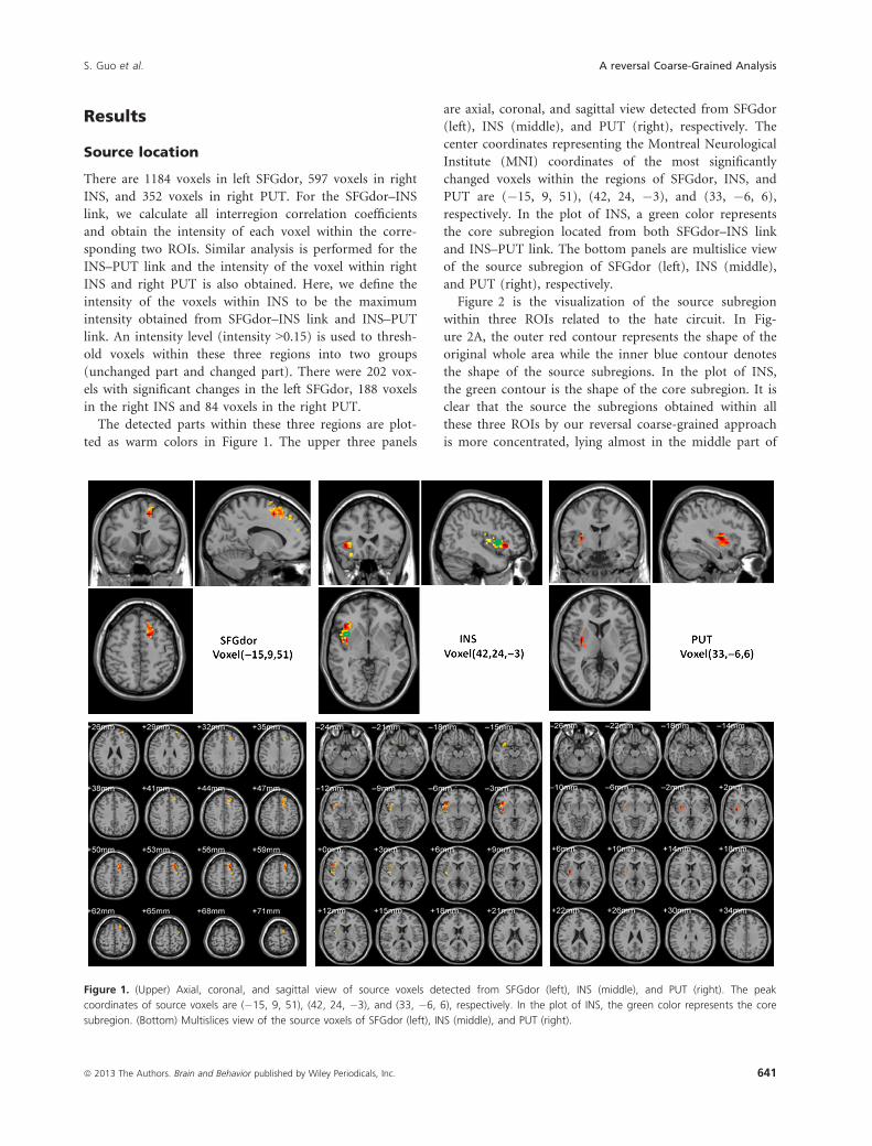
The detected parts within these three regions are plot-

ted as warm colors in Figure 1. The upper three panels

are axial, coronal, and sagittal view detected from SFGdor

(left), INS (middle), and PUT (right), respectively. The

center coordinates representing the Montreal Neurological

Institute (MNI) coordinates of the most significantly

changed voxels within the regions of SFGdor, INS, and

PUT are (�15, 9, 51), (42, 24, �3), and (33, �6, 6),

respectively. In the plot of INS, a green color represents

the core subregion located from both SFGdor–INS link

and INS–PUT link. The bottom panels are multislice view

of the source subregion of SFGdor (left), INS (middle),

and PUT (right), respectively.

Figure 2 is the visualization of the source subregion

within three ROIs related to the hate circuit. In Fig-

ure 2A, the outer red contour represents the shape of the

original whole area while the inner blue contour denotes

the shape of the source subregions. In the plot of INS,

the green contour is the shape of the core subregion. It is

clear that the source the subregions obtained within all

these three ROIs by our reversal coarse-grained approach

is more concentrated, lying almost in the middle part of

Figure 1. (Upper) Axial, coronal, and sagittal view of source voxels detected from SFGdor (left), INS (middle), and PUT (right). The peak

coordinates of source voxels are (�15, 9, 51), (42, 24, �3), and (33, �6, 6), respectively. In the plot of INS, the green color represents the core

subregion. (Bottom) Multislices view of the source voxels of SFGdor (left), INS (middle), and PUT (right).



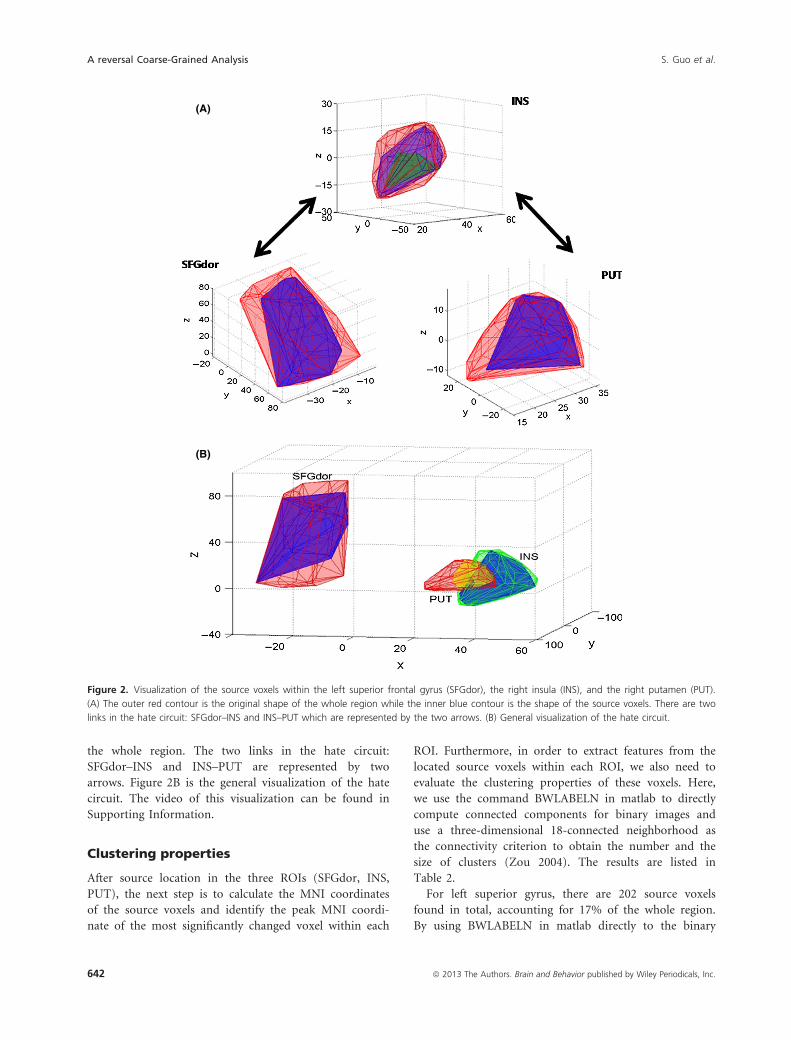
the whole region. The two links in the hate circuit:

SFGdor–INS and INS–PUT are represented by two

arrows. Figure 2B is the general visualization of the hate

circuit. The video of this visualization can be found in

Supporting Information.

Clustering properties

After source location in the three ROIs (SFGdor, INS,

PUT), the next step is to calculate the MNI coordinates

of the source voxels and identify the peak MNI coordi-

nate of the most significantly changed voxel within each

ROI. Furthermore, in order to extract features from the

located source voxels within each ROI, we also need to

evaluate the clustering properties of these voxels. Here,

we use the command BWLABELN in matlab to directly

compute connected components for binary images and

use a three-dimensional 18-connected neighborhood as

the connectivity criterion to obtain the number and the

size of clusters (Zou 2004). The results are listed in

Table 2.

For left superior gyrus, there are 202 source voxels

found in total, accounting for 17% of the whole region.

By using BWLABELN in matlab directly to the binary

(A)

(B)

Figure 2. Visualization of the source voxels within the left superior frontal gyrus (SFGdor), the right insula (INS), and the right putamen (PUT).

(A) The outer red contour is the original shape of the whole region while the inner blue contour is the shape of the source voxels. There are two

links in the hate circuit: SFGdor–INS and INS–PUT which are represented by the two arrows. (B) General visualization of the hate circuit.



image, we obtain eight clusters. The largest cluster has

164 voxels with peak MNI coordinate being (�15, 9, 51)

and peak intensity is 0.536 with P = 0.0175. The second

largest cluster has 14 voxels and third largest cluster has 7

voxels and the fourth cluster have 4 voxels and the

remaining one cluster has only 1 voxel.

In the right INS, there are altogether 188 source voxels,

which account for 31% of the whole region. We obtain

nine clusters with the largest one having 178 voxels, peak

MNI coordinate being (42, 24, �3), and peak intensity is

0.55,398 with P = 0.0197. The next two clusters have 2

voxels and the remaining six clusters have 1 voxel. The

core of the subregion includes 11 voxels, all of which are

located in the largest cluster.

In the right PUT, there are 84 source voxels in total,

account for 25% of the whole region. We obtain three

clusters with the largest having 81 voxels, peak MNI coor-

dinate being (33, �6, 6), and peak intensity is 0.3417 with

P = 0.0397. The remaining one cluster has 2 voxels with

peak MNI coordinate being (27, �15, 6) and one cluster

contains 1 voxel with MNI coordinate being (27, 18, �6).

Comparisons on various statistics

After locating source subregions of the hate circuit, the

voxel-wise time series, that is, the averaged time series

over the identified source, voxels within each ROI can be

obtained for further analysis. To compare the ROI-wise

time series and the voxel-wise time series in analyzing the

two links SFGdor–INS and INS–PUT, for each subject,

we plot the correlation coefficients of the two functional

connectivity (SFGdor–INS and INS–PUT) using the ROI-

wise data and the voxel-wise data, respectively (see

Fig. 3A). It can be seen that the correlation coefficients of

these two links calculated using ROI-wise data are slightly

higher than those obtained using the voxel-wise data both

for patients and controls. This observation indicates the

reduction of the coherence of activity among the three

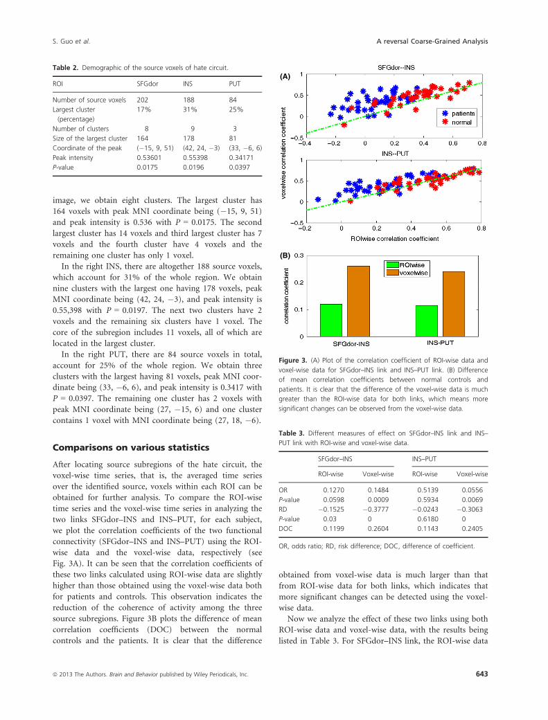
source subregions. Figure 3B plots the difference of mean

correlation coefficients (DOC) between the normal

controls and the patients. It is clear that the difference

obtained from voxel-wise data is much larger than that

from ROI-wise data for both links, which indicates that

more significant changes can be detected using the voxel-

wise data.

Now we analyze the effect of these two links using both

ROI-wise data and voxel-wise data, with the results being

listed in Table 3. For SFGdor–INS link, the ROI-wise data

(A)

(B)

Figure 3. (A) Plot of the correlation coefficient of ROI-wise data and

voxel-wise data for SFGdor–INS link and INS–PUT link. (B) Difference

of mean correlation coefficients between normal controls and

patients. It is clear that the difference of the voxel-wise data is much

greater than the ROI-wise data for both links, which means more

significant changes can be observed from the voxel-wise data.

Table 2. Demographic of the source voxels of hate circuit.

ROI SFGdor INS PUT

Number of source voxels 202 188 84

Largest cluster

(percentage)

17% 31% 25%

Number of clusters 8 9 3

Size of the largest cluster 164 178 81

Coordinate of the peak (�15, 9, 51) (42, 24, �3) (33, �6, 6)

Peak intensity 0.53601 0.55398 0.34171

P-value 0.0175 0.0196 0.0397

Table 3. Different measures of effect on SFGdor–INS link and INS–

PUT link with ROI-wise and voxel-wise data.

SFGdor–INS INS–PUT

ROI-wise Voxel-wise ROI-wise Voxel-wise

OR 0.1270 0.1484 0.5139 0.0556

P-value 0.0598 0.0009 0.5934 0.0069

RD �0.1525 �0.3777 �0.0243 �0.3063

P-value 0.03 0 0.6180 0

DOC 0.1199 0.2604 0.1143 0.2405

OR, odds ratio; RD, risk difference; DOC, difference of coefficient.



have an odds ratio of 0.1270 with P = 0.0598, while

voxel-wise data have an odds ratio of 0.1484 with

P = 0.0009, which is far more significant than that from

ROI-wise data. For the absolute measure of effect, the

ROI-wise data have a risk difference of �0.1525 with

P = 0.03 (permutation test), while voxel-wise data have a

much greater risk difference of �0.3777 with P-value

being almost zero. Similarly, for INS–PUT link, the ROI-

wise data have an odds ratio of 0.5139 with P = 0.5934,

which is no longer significant. But for voxel-wise data,

the corresponding odds ratio is 0.0556 with P = 0.0069,

which is significant. For the absolute measure of effect,

the ROI-wise data have a risk difference of �0.0243 with

P = 0.6180 (permutation test), while voxel-wise data have

a much greater risk difference of �0.3063 with P

approaching zero.

ALFF

After band-pass filtering (0.01–0.08 Hz) and linear-trend

removal, the ROI-wise time series obtained from

coarse-grained analysis and the voxel-wise time series

obtained from reversal coarse-grained analysis can be

extracted. Both of them are transformed to the frequency

domain using a fast Fourier transform and the ALFF can

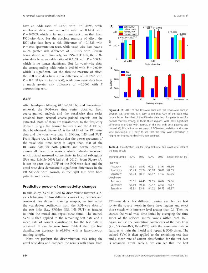
thus be obtained. Figure 4A is the ALFF of the ROI-wise

data and the voxel-wise data in SFGdor, INS, and PUT.

From Figure 4A, it is obvious that the power spectrum of

the voxel-wise time series is larger than that of the

ROI-wise data for both patients and normal controls

among all these three regions, which indicates increased

synchronized neuronal connectivity in located subregions

(Fox and Raichle 2007; Lui et al. 2010). From Figure 4A,

it can be seen that ALFF of the ROI-wise data and the

voxel-wise data demonstrate significant differences in the

left SFGdor with normal, in the right INS with both

patients and normal.

Predictive power of connectivity changes

In this study, SVM is used to discriminate between sub-

jects belonging to two different classes (i.e., patients and

controls). For different training samples, we first select

the correlation coefficients from the ROI-wise data of

the two links (i.e., SFGdor–INS, INS–PUT) as features

to train the model and repeat 5000 times. The trained

SVM is then applied to the remaining test data and a

mean rate of correct classification for the test data is

obtained. It can be seen from Table 4 that the best

classification accuracy is 63.96% with a leave-one-out

training sample.

Next, we perform the discrimination task using the

voxel-wise data and compare the results with those from

ROI-wise data. For different training samples, we first

locate the source voxels in these three regions and select

those voxels with intensity level greater than 0.1. Then we

extract the voxel-wise time series by averaging the time

series of the selected source voxels within each ROI.

Again we use the correlation coefficients of the two links

(i.e., SFGdor–INS, INS–PUT) with the voxel-wise data as

features to train the model and repeat it 5000 times. The

trained SVM is then applied to the remaining test data

and a mean rate of correct classification for the test data

is obtained. From Table 4, we can see that the best

(A)

(B)

400

200

0

80%

70%

60%

50%

SFGdor INSSVM classifier

ALF

Fac

cura

cy

training sample

PUT

40 50 60 70 leave one out

ROIVoxel

patient, ROI

normal, ROIpatient, voxel

normal, voxelp = 0.1795 p = 0.0013

p = 0.0219 p = 0.0012

p = 0.5583p = 0.0688

Figure 4. (A) ALFF of the ROI-wise data and the voxel-wise data in

SFGdor, INS, and PUT. It is easy to see that ALFF of the voxel-wise

data is larger than that of the ROI-wise data both for patients and for

normal controls among all these three regions. ALFF have significant

difference in SFGdor with normal, in the INS with both patients and

normal. (B) Discrimination accuracy of ROI-wise correlation and voxel-

wise correlation. It is easy to see that the voxel-wise correlation is

helpful for improving discrimination accuracy.

Table 4. Classification results using ROI-wise and voxel-wise links of

the hate circuit.

Training sample 40% 50% 60% 70% Leave one out (%)

ROI-wise

Accuracy 56.61 58.92 60.5 61.91 63.96

Specificity 50.43 52.94 56.18 58.89 62.55

Sensitivity 65.93 68.11 68.17 67.52 69.05

Voxel-wise

Accuracy 73.51 74.46 74.95 76.82 77.96

Specificity 66.89 69.36 70.47 72.66 73.67

Sensitivity 83.91 83.84 84.02 86.53 82.97



classification accuracy is increased to 77.96% with a 14%

enhancement of accuracy being obtained. Figure 4B is the

bar plot of the discrimination accuracy with a different

percentage of training samples. It is easy to see that the

voxel-wise data is helpful for improving discrimination

accuracy.

Discussion

Coarse-grained analysis is a general approach that is used

to study the functional connectivity of fMRI data by

dividing the brain into coarse components (ROIs). Using

coarse-grained analysis, one can detect the ROIs or the

functional connectivity with significant differences

between two groups (Ogawa et al. 1990, 1992; Bassett

et al. 2009; Bullmore and Sporns 2009). Previously, the

AAL used by us, similar to those reported in many other

published papers, showed that one ROI may contain a

few thousand voxels and the functional meaning of each

ROI is very complex or is a mixture of different

functions. Coarse-grained analysis may not provide clear

information over these fine spatial scales. Therefore, to

identify the essential differences between two groups and

specify the biological function for each ROI, we moved a

step forward and performed a reversal coarse-grained

analysis that would be more informative for disease

diagnosis.

In the current paper, a reversal coarse-grained analysis

was performed in patients with MDD and matched

healthy controls to determine the exact location of the

changed site of the functional network described in our

previous study. Subregions with the greatest changes

were located within three ROIs, that is, left SFGdor,

right INS, and right PUT. Previous work has shown that

the default mode of network in patients with MDD had

undergone significant changes (Greicius et al. 2003;

Sheline et al. 2009) in the subcortical area (Goldapple

et al. 2004; Zhang et al. 2008; Anand et al. 2009), INS

(Liu et al. 2010), and PUT (Husain et al. 1991; Strakow-

ski et al. 1999, 2002). In our current research, although

reversal coarse-grained analyses focused specifically on

the regions related to the hate circuit, the approach

could be easily applied to other circuits or dysfunctional

regions.

Here, we proposed a holistic method to locate the

source regions by computing the intensity of each voxel.

This is logical because the value of intensity represents

the significance of alteration in the functional connectivity

for each voxel. The measure of intensity is superior to

merely thresholding the intervoxel correlation coefficients

by P-values, as the functional connectivity of two voxels

is very sensitive to noise which is ineluctable in our fMRI

signal (Friman et al. 2003; Polyn et al. 2005). Another

approach to select source voxels was based on the level of

information about the patterns of activity expressed over

all possible sets of voxels (Norman et al. 2006). Because

of the combinatorial explosion issue caused by the large

number of possible voxel sets, this approach can be

improved further in different ways. Kriegeskorte et al.

(2006) proposed scanning the image volume using a

“searchlight” and limiting the search to sets of spatially

adjacent voxels. All spherical searchlights were assumed to

become active as a unit. Different region sizes (the radius

of the spherical “searchlight”) were first checked to yield

the optimal performance of the “searchlight.” The

“searchlight” was then obtained by computing the multi-

variate effect statistic at each location. Pessoa and

Padmala (2007) used an iterative procedure by deleting 1

voxel from the set each time to maximize the goodness of

the current voxel set. Their basic idea was to start with all

voxels and iteratively eliminate the “least informative”

voxel (i.e., the smallest weight) at each cycle. This process

was repeated until there was no need to delete voxels.

Obviously, this method is more time consuming com-

pared with our approach.

Our results demonstrated that the voxel-wise time

series extracted from reversal coarse-grained analysis have

a few advantages over ROI-wise time series extracted

from coarse-grained analysis. First, the voxel-wise time

series had larger ALFFs for all three areas related to the

hate circuit (Fig. 4A). In previous studies, ALFF was

thought to reflect spontaneous neural activity (Fox and

Raichle 2007), which was correlated with activity in

gamma-band power (Shmuel and Leopold 2008); this in

turn reflects increased regionally synchronized neuronal

connectivity and is associated with a capacity for higher

cognitive functions (Lewis et al. 2008). The enhancement

of ALFF reflects that the regional neuronal populations

function in a more synchronous manner within the

source subregions than in the entire region. Second, a

reversal coarse-grained analysis resulted in the attenuation

of functional connectivity, both for the SFGdor–INS and

INS–PUT connectivities (Fig. 3A), probably because the

localized subregions led to a reduction of the integration

of synchronous activity across brain regions. The greater

difference of these two links between the two groups indi-

cated that a more significant difference could be detected.

However, it is unclear whether this reduced connectivity

is beneficial. The pattern of increased ALFF, together with

reduced network level connectivity, suggests that

increased spontaneous regional neural activity is associ-

ated with a parallel reduction, rather than with an

enhancement in the coherence of activity across the three

source regions (SFGdor, INS, and PUT). Third, reversal

coarse-grained analysis had a greater effect (in terms of

both odds ratio and risk difference) on functional



connectivity (SFGdor–INS and INS–PUT); this means

that the identified subregions exhibited significant differ-

ences between the two groups.

Our discrimination results showed that feature selec-

tion, based on reversal coarse-grained analysis, yields a

better classification performance. In fact, many discrimi-

nation analyses performed at the voxel level yielded high

discrimination accuracy. For example, a classification

method was proposed to distinguish subjects of two

groups using multiple independent components and their

combinations, with the independent component extracted

on the basis of the time series of each voxel (Calhoun

et al. 2008; Demirci et al. 2008). Although different inde-

pendent components had different classification perfor-

mances, the selection of independent components relied

on a priori knowledge, and no systematic component

selection method was available. Another frequently used

discrimination approach is multivoxel pattern analysis

(MVPA), which uses pattern-classification techniques to

extract the signal across multiple voxels. Many studies

have used MVPA to discriminate cognitive changes

successfully. For example, MVPA has been used to predict

the time course of recall behavior in a free-recall task

(Polyn et al. 2005), and it has also been used to predict

second-by-second changes in perceived stimulus domi-

nance during a binocular rivalry task (Haynes and Rees

2005). The most important obstacle to the extensive use

of the voxel-based discrimination approach is the large

number of voxel sets to be scanned. However, if improve-

ments are made in the computational algorithms, the

voxel-based approach will be highly promising as a tool

for characterizing and understanding of how information

is represented and processed in the brain.

In functional connectivity analysis, the term ROI-wise

or voxel-wise is occasionally used in different documents

or software (e.g., in Resting-State fMRI Data Analysis

Toolkit (REST) provided by Beijing Normal University

(http://www.restfmri.net/), one can calculate ROI-wise or

voxel-wise functional connectivity directly), indicating

that both ROI-wise analysis and voxel-wise analysis in

functional connectivity are seed-based approaches. The

ROI-wise analysis estimates the brain connectivity by

computing correlation between temporal signals from

two predefined ROIs, whereas the voxel-wise analysis

correlates functional temporal signals of a seed region

with those of other brain voxels (Craddock et al. 2011;

Valsasina et al. 2011). The selection of ROIs typically

requires a priori knowledge about the underlying prob-

lem; therefore, both of these approaches are conceptually

different from the reversal coarse-grained method

proposed here.

In summary, the current study compared coarse-

grained analysis with reversal coarse-grained analysis by

analyzing the functional abnormalities of the hate circuit

studied previously by us in patients with MDD over a

fine spatial scale (Tao et al. 2011). By computing the

intensity of each voxel, we were able to precisely localize

the changed site of the hate circuit. Furthermore, our

results demonstrated that the voxel-wise time series

extracted from the reversal coarse-grained analysis had

several advantages: (1) a larger amplitude of fluctuations

was detected, which indicates that the BOLD signals are

more synchronized; (2) more significant differences were

observed in the functional connectivity related to the

ROIs between patients and controls; and (3) a better per-

formance was observed in the discrimination tasks. From

a global perspective, coarse-grained analysis is an appro-

priate method to investigate the significantly different

ROIs and functional connectivity. However, to determine

the essential, clinically relevant difference between patients

and healthy controls, a reversal coarse-grained analysis

should be carried out to identify functional and, possibly,

anatomical abnormalities in greater detail.

Acknowledgment

J. F. F. is a Royal Society Wolfson Research Merit Award

holder, partially supported by National Centre for Mathe-

matics and Interdisciplinary Sciences (NCMIS) of the

Chinese Academy of Sciences and Key Program of

National Natural Science Foundation of China (No.

91230201). S. X. G. is supported by the National Natural

Science Foundation of China (NSFC) grant: 11271121,

Program for New Century Excellent Talents in University

(NCET) grant, Key Laboratory of Computational and

Stochastic Mathematics and Its Application of Hunan

province (11K038) and the Construct Program of the Key

Discipline in Hunan Province. J. Z. is supported by grants

from the Natural Scientific Foundation of China

(61104143 and 61004104).

Conflict of Interest

None declared.

References

Anand, A., Y. Li, Y. Wang, J. Wu, S. Gao, and L. Bukhari.

2005. Antidepressant effect on connectivity of the

mood-regulating circuit: an FMRI study.

Neuropsychopharmacology 30:1334–1344.

Anand, A., Y. Li, Y. Wang, M. J. Lowe, and M. Dzemidzic.

2009. Resting state corticolimbic connectivity abnormalities

in unmedicated bipolar disorder and unipolar depression.

Psychiatry Res. 171:189–198.

Bassett, D. S., E. T. Bullmore, Andreas Meyer-Lindenberg,

A. A. Jos�e, R. W. Daniel, and C. Richard. 2009. Cognitive



fitness of cost-efficient brain functional networks. Proc.

Natl. Acad. Sci. USA 106:11747–11752.

Bland, J. M., and D. G. Altman. 2000. Statistics notes: the

odds ratio. BMJ 320(7247):1468.

Bullmore, E. D., and O. Sporns. 2009. Complex brain

networks: graph theoretical analysis of structural and

functional systems. Nat. Rev. Neurosci. 10:186–198.

Calhoun, V. D., P. K. Maciejewski, G. D. Pearlson, and

K. A. Kiehl. 2008. Temporal lobe and “default” hemodynamic

brain modes discriminate between schizophrenia and bipolar

disorder. Hum. Brain Mapp. 29:1265–1275.

Craddock, R. C., G. A. James, P. E. Holtzheimer III , X. P.

Hu, and M. S. Mayberg. 2011. A whole brain fMRI atlas

generated via spatially constrained spectral clustering. Hum.

Brain Mapp. 33:1914–1928.

Demirci, O., V. P. Clark, and V. D. Calhoun. 2008. A

projection pursuit algorithm to classify individuals using

fMRI data: application to schizophrenia. Neuroimage

39:1774–1782.

Dosenbach, N. U., B. Nardos, A. L. Cohen, D. A. Fair,

J. D. Power, J. A. Church, et al. 2010. Prediction of

individual brain maturity using fMRI. Science

329:1358–1361.

Fox, M. D., and M. E. Raichle. 2007. Spontaneous fluctuations

in brain activity observed with functional magnetic

resonance imaging. Nat. Rev. Neurosci. 8:700–711.

Friman, O., M. Borga, P. Lundberg, and H. Knutsson. 2003.

Adaptive analysis of fMRI data. Neuroimage 19:837–845.

Goldapple, K., Z. Segal, C. Garson, M. Lau, P. Bieling, S.

Kennedy, et al. 2004. Modulation of cortical-limbic

pathways in major depression. Arch. Gen. Psychiatry

61:34–41.

Greicius, M. D., B. Krasnow, A. L. Reiss, and V. Menon. 2003.

Functional connectivity in the resting brain: a network

analysis of the default mode hypothesis. Proc. Natl. Acad.

Sci. USA 100:253–258.

Guo, S. X., K. M. Kendrick, R. J. Yu, H.-L. S. Wang, and

J. F. Feng. 2012. Key functional circuitry altered in

schizophrenia involves parietal regions associated with sense

of self. Hum. Brain Mapp. doi: 10.1002/hbm.22162

Hastie, T., R. Tibshirani, and J. Friedman. 2001. The elements

of statistical learning: data mining, inference, and

prediction. Springer, New York, NY.

Haynes, J. D., and G. Rees. 2005. Predicting the stream of

consciousness from activity in human visual cortex. Curr.

Biol. 15:1301–1307.

Humphreys, K., N. Minshew, G. L. Leonard, and M.

Behrmann. 2007. A fine-grained analysis of facial expression

processing in high-functioning adults with autism.

Neuropsychologia 45:685–695.

Husain, M. M., W. M. McDonald, P. M. Doraiswamy, G. S.

Figiel, C. Na, P. Escalona, et al. 1991. A magnetic resonance

imaging study of putamen nuclei in major depression.

Psychiatry Res. 40:95–99.

Kempton, M. J., Z. Salvador, M. R. Munaf�o, J. R. Geddes, A.

Simmons, S. Frangou, et al. 2011. Structural neuroimaging

studies in major depressive disorder: meta-analysis and

comparison with bipolar disorder. Arch. Gen. Psychiatry

68(7):675–90.

Kimbrell, T. A., T. A. Ketter, M. S. George, J. T. Little,

B. E. Benson, M. W. Willis, et al. 2002. Regional

cerebral glucose utilization in patients with a range of

severities of unipolar depression. Biol. Psychiatry 51:237–

252.

Kriegeskorte, N., R. Goebel, and P. Bandettini. 2006.

Information-based functional brain mapping. Proc. Natl.

Acad. Sci. USA 103:3863–3868.

Kriegeskorte, N., R. Cusack, and P. Bandettini. 2010. How

does an fMRI voxel sample the neuronal activity pattern:

compact-kernel or complex spatiotemporal filter?

Neuroimage 49:1965–1976.

LaConte, S., S. Strother, V. Cherkassky, J. Anderson, and

X. P. Hu. 2005. Support vector machines for temporal

classification of block design fMRI data. Neuroimage

26:317–329.

Lewis, D. A., R. Y. Cho, C. S. Carter, K. Eklund, S. Forster,

M. A. Kelly, et al. 2008. Subunit-selective modulation of

GABA type a receptor neurotransmission and cognition in

schizophrenia. Am. J. Psychiatry 165:1585–1593.

Liu, Z. F., C. Xu, Y. Xu, Y. F. Wang, B. Zhao, Y. T. Lv, et al.

2010. Decreased regional homogeneity in insula and

cerebellum: a resting-state fMRI study in patients with

major depression and subjects at high risk for major

depression. Psychiatry Res. 182:211–215.

Lui, S., T. Li, W. Deng, L. Jiang, Q. Wu, H. Tang, et al. 2010.

Short-term effects of antipsychotic treatment on cerebral

function in drug-naive first-episode schizophrenia revealed

by “resting state” functional magnetic resonance imaging.

Arch. Gen. Psychiatry 67:783–792.

Maldjian, J. A., P. J. Laurienti, J. B. Burdette, and R. A. Kraft.

2003. An automated method for neuroanatomic and

cytoarchitectonic atlas-based interrogation of fMRI data sets.


Mour~ao-Miranda, J., K. J. Friston, and M. Brammer. 2007.

Dynamic discrimination analysis: a spatial–temporal SVM.


Norman, K. A., S. M. Polyn, G. J. Detre, and J. V. Haxby.

2006. Beyond mind-reading: multi-voxel pattern analysis of

fMRI data. Trends Cogn. Sci. 10:424–430.

Ogawa, S., T. M. Lee, A. R. Kay, and D. W. Tank. 1990. Brain

magnetic resonance imaging with contrast dependent on

blood oxygenation. Proc. Natl. Acad. Sci. USA

87:9868–9872.

Ogawa, S., D. W. Tank, R. Menon, J. M. Ellermann,

S. G. Kim, H. Merkle, et al. 1992. Intrinsic signal changes

accompanying sensory stimulation: functional brain

mapping with magnetic resonance imaging. Proc. Natl.

Acad. Sci. USA 89:5951–5955.



Pepe, M. S., H. Janes, G. Longton, W. Leisenring, and

P. Newcomb. 2004. Limitations of the odds ratio in gauging

the performance of a diagnostic, prognostic, or screening

marker. Am. J. Epidemiol. 159:882–890.

Pessoa, L., and S. Padmala. 2007. Decoding near-threshold

perception of fear from distributed single-trial brain

activation. Cereb. Cortex 17:691–701.

Polyn, S. M., V. S. Natu, F. D. Cohen, and K. A. Norman.

2005. Category-specific cortical activity precedes retrieval

during memory search. Science 310:1963–1966.

Sheline, Y. I., D. M. Barch, J. L. Price, M. M. Rundle,

S. N. Vaishnavi, A. Z. Snyder, et al. 2009. The default mode

network and self-referential processes in depression. Proc.

Natl. Acad. Sci. USA 106:1942–1947.

Shmuel, A., and D. A. Leopold. 2008. Neuronal correlates of

spontaneous fluctuations in fMRI signals in monkey visual

cortex: implications for functional connectivity at rest.

Hum. Brain Mapp. 29:751–761.

Strakowski, S. M., M. P. DelBello, K. W. Sax,

M. E. Zimmerman, P. K. Shear, J. M. Hawkins, et al. 1999.

Brain magnetic resonance imaging of structural

abnormalities in bipolar disorder. Arch. Gen. Psychiatry

56:254–260.

Strakowski, S. M., M. P. DelBello, M. E. Zimmerman,

G. E. Getz, M. P. Mills, J. Ret, et al. 2002. Ventricular and

periventricular structural volumes in first-versus

multiple-episode bipolar disorder. Am. J. Psychiatry

159:1841–1847.

Tao, H. J., S. X. Guo, T. Ge, K. M. Kendrick, Z. M. Xue, Z. N.

Liu, et al. 2011. Depression uncouples brain hate circuit.

Mol. Psychiatry 18:101–111. doi: 10.1038/mp.2011.127

Tripepi, G., K. G. Jager, F. W. Dekker, C. Wanner, and

C. Zoccali. 2007. Measures of effect: relative risks, odds

ratios, risk difference, and “number needed to treat.” Kidney

Int. 72:789–791.

Tzourio-Mazoyer, N., B. Landeau, D. Papathanassiou,

F. Crivello, O. Etard, N. Delcroix, et al. 2002. Automated

anatomical labeling of activations in SPM using a

macroscopic anatomical parcellation of the MNI MRI

single-subject brain. Neuroimage 15:273–289.

Valsasina, P., M. A. Rocca, M. Absinta, M. P. Sormani,

L. Mancini, N. D. Stefano, et al. 2011. A multicentre study

of motor functional connectivity changes in patients with

multiple sclerosis. Eur. J. Neurosci. 33:1256–1263.

Wacholder, S. 1986. Binomial regression in glim: estimating

risk ratios and risk difference. Am. J. Epidemiol.

123:174–184.

Yan, C. G., and Y. F. Zang. 2010. DPARSF: a MATLAB

toolbox for “Pipeline” data analysis of resting-state fMRI.

Front. Syst. Neurosci. 4:00013.

Yang, H., X. Y. Long, Y. H. Yang, H. Yan, C. Z. Zhu,

X. P. Zhou, et al. 2007. Amplitude of low frequency

fluctuation within visual areas revealed by resting-state

functional MRI. Neuroimage 36:144–152.

Zhang, D., A. Z. Snyder, M. D. Fox, M. W. Sansbury,

J. S. Shimony, and M. E. Raichle. 2008. Intrinsic functional

relations between human cerebral cortex and thalamus.

J. Neurophysiol. 100:1740.

Zhang, J., W. Cheng, Z. Wang, Z. Zhang, W. Lu, G. Lu, et al.

2012. Pattern classification of large-scale functional brain

networks: identification of informative neuroimaging

markers for epilepsy. PLoS ONE 7:e36733.

Zou, G. Y. 2004. A modified poisson regression approach to

prospective studies with binary data. Am. J. Epidemiol.

159:702–706.

Supporting Information

Additional Supporting Information may be found in the

online version of this article:

Data S1. INS_all.xlsx: coordinate of all INS voxels.

Data S2. INS_small.xlsx: coordinate of source INS voxel.

Data S3. PUT_all xlsx: coordinate of all PUT voxels.

Data S4. PUT_small.xlsx: coordinate of sourcel PUT voxels.

Data S5. SFGdor_all. xlsx: coordinate of all SFGdor voxels.

Data S6. SFGdor_small.xlsx: coordinate of source SFGdor

voxels.

Data S7. Myrotate: code for Figure 2.

Data S8. Video: code for Figure 2.

Data S9. Code for brain-wise association study (BWAS)

Data S10. Code for brain-wise association study (BWAS).














Documents

A reversal coarsegrained analysis with application to an ...wrap.warwick.ac.uk/57406/1/WRAP_Feng_brb3173.pdf · analysis with application to an altered functional circuit in depression