A Review of Bayesian Variable Selection - NCSU Statistics

A Review of Bayesian VariableSelection

By: Brian J Reich and Sujit Ghosh,North Carolina State University

E-mail:[email protected]

Slides, references, and BUGS code are on my webpage,http://www4.stat.ncsu.edu/∼reich/.

Brian Reich Bayesian variable selection

Why Bayesian variable selection?

I Bayesian variable selection methods come equipped withnatural measures of uncertainty, such as the posteriorprobability of each model and the marginal inclusionprobabilities of the individual predictors.

I Stochastic variable search is extremely flexible and has beenapplied in a wide range of applications.

I Model uncertainly can be incorporated into prediction throughmodel averaging, which usually improves prediction.

I Given the model (likelihood, prior, and loss function), thereare formal justifications for choosing a particular model.

I Missing data is easily handled by MCMC.


Drawbacks of Bayesian methods

Computational issues:I For the usual regression setting, the “BMA” (Bayesian Model

Averaging) package in R can be used for Bayesian variableselection.

I WinBUGS is a free user-friendly software package that can beused for stochastic variable search.

Prior selection:I Bayesian variable selection can be influenced by the prior.

I Priors can be chosen to mimic Frequentist solutions (Yuanand Lin).

I Priors can be derived to have large sample properties(Ishwaran and Rao).


Notation

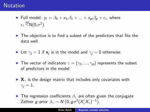
I Full model: yi = β0 + x1iβ1 + ... + xpiβp + εi , where

εiiid∼N(0,σ2).

I The objective is to find a subset of the predictors that fits thedata well.

I Let γj = 1 if xj is in the model and γj = 0 otherwise.

I The vector of indicators γ = (γ1, ..., γp) represents the subsetof predictors in the model.

I Xγ is the design matrix that includes only covariates withγj = 1.

I The regression coefficients βγ are often given the conjugateZellner g -prior βγ ∼ N

(0, gσ2(X ′

γXγ)−1).


Bayes Factors

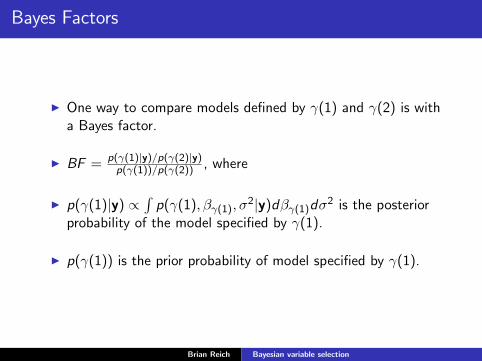
I One way to compare models defined by γ(1) and γ(2) is witha Bayes factor.

I BF = p(γ(1)|y)/p(γ(2)|y)p(γ(1))/p(γ(2)) , where

I p(γ(1)|y) ∝ ∫p(γ(1), βγ(1), σ

2|y)dβγ(1)dσ2 is the posteriorprobability of the model specified by γ(1).

I p(γ(1)) is the prior probability of model specified by γ(1).


BIC approximation

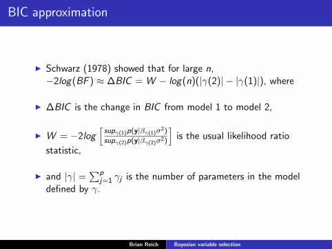
I Schwarz (1978) showed that for large n,−2log(BF ) ≈ ∆BIC = W − log(n)(|γ(2)| − |γ(1)|), where

I ∆BIC is the change in BIC from model 1 to model 2,

I W = −2log[

supγ(1)p(y|βγ(1)σ2)

supγ(2)p(y|βγ(2)σ2)

]is the usual likelihood ratio

statistic,

I and |γ| = ∑pj=1 γj is the number of parameters in the model

defined by γ.


BIC approximation

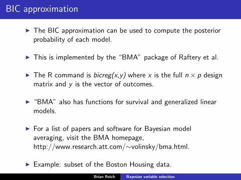
I The BIC approximation can be used to compute the posteriorprobability of each model.

I This is implemented by the “BMA” package of Raftery et al.

I The R command is bicreg(x,y) where x is the full n× p designmatrix and y is the vector of outcomes.

I “BMA” also has functions for survival and generalized linearmodels.

I For a list of papers and software for Bayesian modelaveraging, visit the BMA homepage,http://www.research.att.com/∼volinsky/bma.html.

I Example: subset of the Boston Housing data.


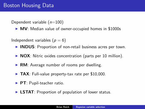
Boston Housing Data

Dependent variable (n=100)

I MV: Median value of owner-occupied homes in $1000s

Independent variables (p = 6)

I INDUS: Proportion of non-retail business acres per town.

I NOX: Nitric oxides concentration (parts per 10 million).

I RM: Average number of rooms per dwelling.

I TAX: Full-value property-tax rate per $10,000.

I PT: Pupil-teacher ratio.

I LSTAT: Proportion of population of lower status.


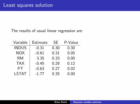
Least squares solution

The results of usual linear regression are:

Variable Estimate SE P-Value

INDUS -0.31 0.30 0.30NOX -0.61 0.31 0.05RM 3.35 0.33 0.00TAX -0.45 0.28 0.12PT -0.63 0.27 0.02

LSTAT -1.77 0.35 0.00


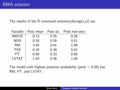
BMA solution

The results of the R command summary(bicreg(x,y)) are:

Variable Post mean Post sd. Prob non-zero


LSTAT -1.93 0.38 1.00

The model with highest posterior probability (prob = 0.20) hasRM, PT, and LSTAT.


Stochastic variable selection

I A limitation of the Bayes factor approach is that for large p,computing the BIC for all 2p models is impossible.

I Madigan and Raftery (1994) limit the search to a class ofmodels under consideration to models with a minimum levelof posterior support and propose a greedy-search algorithm tofind models with high posterior probability.

I Stochastic variable selection is an alternative.

I Here we use MCMC to draw samples from the model space somodels with high posterior probability will be visited moreoften than low probability models.

I We’ll follow the notation and model of George andMcCullough, JASA, 1993.


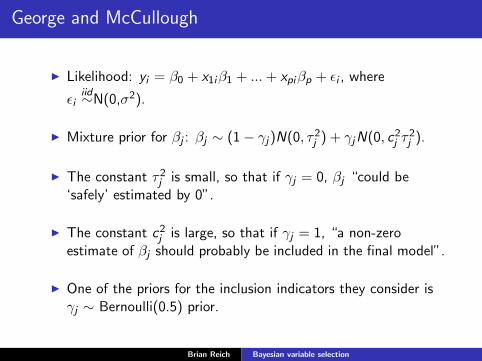
George and McCullough

I Likelihood: yi = β0 + x1iβ1 + ... + xpiβp + εi , where

εiiid∼N(0,σ2).

I Mixture prior for βj : βj ∼ (1− γj)N(0, τ2j ) + γjN(0, c2

j τ2j ).

I The constant τ2j is small, so that if γj = 0, βj “could be

‘safely’ estimated by 0”.

I The constant c2j is large, so that if γj = 1, “a non-zero

estimate of βj should probably be included in the final model”.

I One of the priors for the inclusion indicators they consider isγj ∼ Bernoulli(0.5) prior.


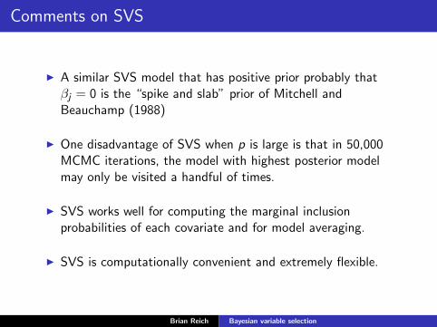
Comments on SVS

I A similar SVS model that has positive prior probably thatβj = 0 is the “spike and slab” prior of Mitchell andBeauchamp (1988)

I One disadvantage of SVS when p is large is that in 50,000MCMC iterations, the model with highest posterior modelmay only be visited a handful of times.

I SVS works well for computing the marginal inclusionprobabilities of each covariate and for model averaging.

I SVS is computationally convenient and extremely flexible.


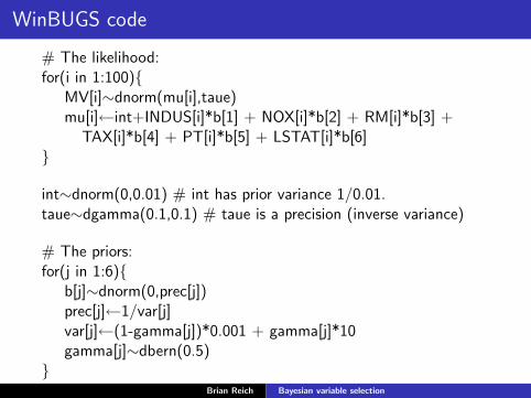
WinBUGS code

# The likelihood:for(i in 1:100){

MV[i]∼dnorm(mu[i],taue)mu[i]←int+INDUS[i]*b[1] + NOX[i]*b[2] + RM[i]*b[3] +

TAX[i]*b[4] + PT[i]*b[5] + LSTAT[i]*b[6]}

int∼dnorm(0,0.01) # int has prior variance 1/0.01.taue∼dgamma(0.1,0.1) # taue is a precision (inverse variance)

# The priors:for(j in 1:6){

b[j]∼dnorm(0,prec[j])prec[j]←1/var[j]var[j]←(1-gamma[j])*0.001 + gamma[j]*10gamma[j]∼dbern(0.5)

}Brian Reich Bayesian variable selection

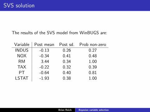
SVS solution

The results of the SVS model from WinBUGS are:

Variable Post mean Post sd. Prob non-zero


LSTAT -1.93 0.38 1.00


More about SVS

Applications of SVS: Choosing the priors for β and γ:

I Connection with the LASSO (Yuan and Li, JASA, 2005)

I Rescaled spike and slab priors of Ishwaran and Rao (Annals,2005).

I Gene selection using microarray data.

I Nonparametric regression for complex computer models


Connection with penalized regression

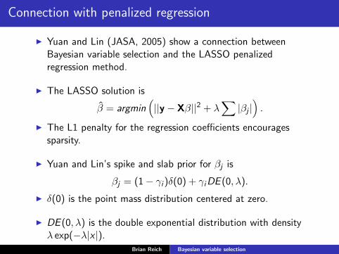
I Yuan and Lin (JASA, 2005) show a connection betweenBayesian variable selection and the LASSO penalizedregression method.

I The LASSO solution is

β̂ = argmin(||y − Xβ||2 + λ

∑|βj |

).

I The L1 penalty for the regression coefficients encouragessparsity.

I Yuan and Lin’s spike and slab prior for βj is

βj = (1− γi )δ(0) + γiDE (0, λ).

I δ(0) is the point mass distribution centered at zero.

I DE (0, λ) is the double exponential distribution with densityλ exp(−λ|x |).


Connection with penalized regression

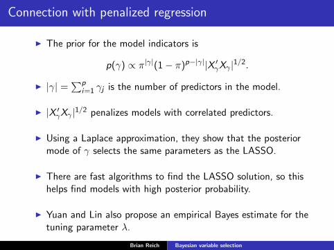
I The prior for the model indicators is

p(γ) ∝ π|γ|(1− π)p−|γ||X ′γXγ |1/2.

I |γ| = ∑pi=1 γj is the number of predictors in the model.

I |X ′γXγ |1/2 penalizes models with correlated predictors.

I Using a Laplace approximation, they show that the posteriormode of γ selects the same parameters as the LASSO.

I There are fast algorithms to find the LASSO solution, so thishelps find models with high posterior probability.

I Yuan and Lin also propose an empirical Bayes estimate for thetuning parameter λ.


Rescaled spike and slab model of Ishwaran and Rao

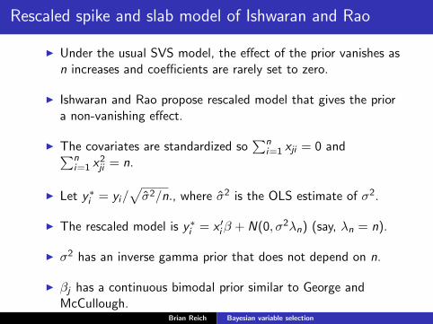
I Under the usual SVS model, the effect of the prior vanishes asn increases and coefficients are rarely set to zero.

I Ishwaran and Rao propose rescaled model that gives the priora non-vanishing effect.

I The covariates are standardized so∑n

i=1 xji = 0 and∑ni=1 x2

ji = n.

I Let y∗i = yi/√

σ̂2/n., where σ̂2 is the OLS estimate of σ2.

I The rescaled model is y∗i = x ′i β + N(0, σ2λn) (say, λn = n).

I σ2 has an inverse gamma prior that does not depend on n.

I βj has a continuous bimodal prior similar to George andMcCullough.


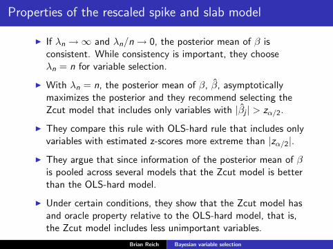
Properties of the rescaled spike and slab model

I If λn →∞ and λn/n → 0, the posterior mean of β isconsistent. While consistency is important, they chooseλn = n for variable selection.

I With λn = n, the posterior mean of β, β̂, asymptoticallymaximizes the posterior and they recommend selecting theZcut model that includes only variables with |β̂j | > zα/2.

I They compare this rule with OLS-hard rule that includes onlyvariables with estimated z-scores more extreme than |zα/2|.

I They argue that since information of the posterior mean of βis pooled across several models that the Zcut model is betterthan the OLS-hard model.

I Under certain conditions, they show that the Zcut model hasand oracle property relative to the OLS-hard model, that is,the Zcut model includes less unimportant variables.


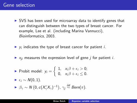
Gene selection

I SVS has been used for microarray data to identify genes thatcan distinguish between the two types of breast cancer. Forexample, Lee et al. (including Marina Vannucci),Bioinformatics, 2003.

I yi indicates the type of breast cancer for patient i .

I xji measures the expression level of gene j for patient i .

I Probit model: yi =

{1, xiβ + εi > 0;0, xiβ + εi ≤ 0.

I εi ∼ N(0, 1).

I βγ ∼ N(0, c(X ′

γXγ)−1), γj

iid∼ Bern(π).


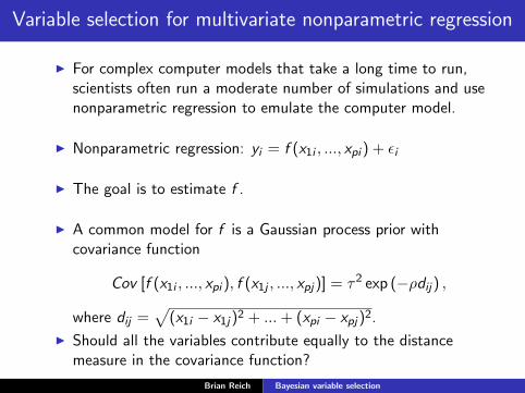
Variable selection for multivariate nonparametric regression

I For complex computer models that take a long time to run,scientists often run a moderate number of simulations and usenonparametric regression to emulate the computer model.

I Nonparametric regression: yi = f (x1i , ..., xpi ) + εi

I The goal is to estimate f .

I A common model for f is a Gaussian process prior withcovariance function

Cov [f (x1i , ..., xpi ), f (x1j , ..., xpj)] = τ2 exp (−ρdij) ,

where dij =√

(x1i − x1j)2 + ... + (xpi − xpj)2.

I Should all the variables contribute equally to the distancemeasure in the covariance function?


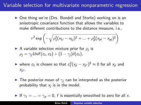
Variable selection for multivariate nonparametric regression

I One thing we’re (Drs. Bondell and Storlie) working on is ananisotropic covariance function that allows the variables tomake different contributions to the distance measure, i.e.,

τ2 exp

(−

√ρ21(x1i − x1j)2 + ... + ρ2

p(xpi − xpj)2)

I A variable selection mixture prior for ρj isρj = γjUnif (c1, c2) + (1− γj)δ(c1),

I where c1 is chosen so that c21 (xji − xji ′)

2 ≈ 0 for all xji andxji ′ .

I The posterior mean of γj can be interpreted as the posteriorprobability that xj is in the model.

I If γ1 = ... = γp = 0, f is essentially smoothed to zero for all x .


Conclusions

I The Bayesian approach to variable selection has severalattractive features, including straight-forward quantification ofvariable importance and model uncertainty and the flexibilityto handle missing data and non-Gaussian distributions.

I Outstanding issues include computational efficiency andconcerns about priors.

I Hopefully we will see some interesting talks about these issuesthroughout the semester.

I THANKS!


Conclusions

I The Bayesian approach to variable selection has severalattractive features, including straight-forward quantification ofvariable importance and model uncertainty and the flexibilityto handle missing data and non-Gaussian distributions.

I Outstanding issues include computational efficiency andconcerns about priors.

I Hopefully we will see some interesting talks about these issuesthroughout the semester.

I THANKS!


Documents

A Review of Bayesian Variable Selection - NCSU Statistics