A Review of Magnetic Sensors

A Review of Magnetic Sensors

JAMES E. LENZ, MEMBER, IEEE

Invited Paper

The techniques used to produce magnetic sensors encompass many aspects of physics and electronics. Eleven of the most common technologies used for magnetic field sensing are described and compared. These are search coil, flux-gate, optically pumped, nuclear precession, SQUlD, Hall-effect, magnetoresis tive, magnetodiode, magnetotransistor, fiber optic, and magneto-optic. The usage of these sensors in relation to working with or around €arth’s magnetic field is also presented.

I. MAGNETIC SENSOR TECHNOLOGIES

Magnetic sensors have assisted mankind in analyzing and controlling thousands of functionsfor many decades. Com- puters have unlimited memorythrough theuseof magnetic sensors in magnetic storage disks and tape drives. Air- planes fly with higher safety standards because of the high reliability of noncontact switching with magnetic sensors. Factories have higher productivity because of the precise stability and low cost of magnetic sensors.

There are many ways to sense magnetic fields, most of them based on the intimate connection between magnetic and electric phenomena. In the first half of this paper, the more popular sensor technologies will be described with examples of products. In the second half, the major applications of magnetic sensors are discussed in relation to three categories: measuring fields stronger than Earth’s field, measuring perturbations in Earth‘s field, and measuring gradients in generated or induced magnetic fields. A common theme among all applications i s that magnetic sensors provide a more rugged, reliable, and maintenance- free technology compared to other sensor technologies.

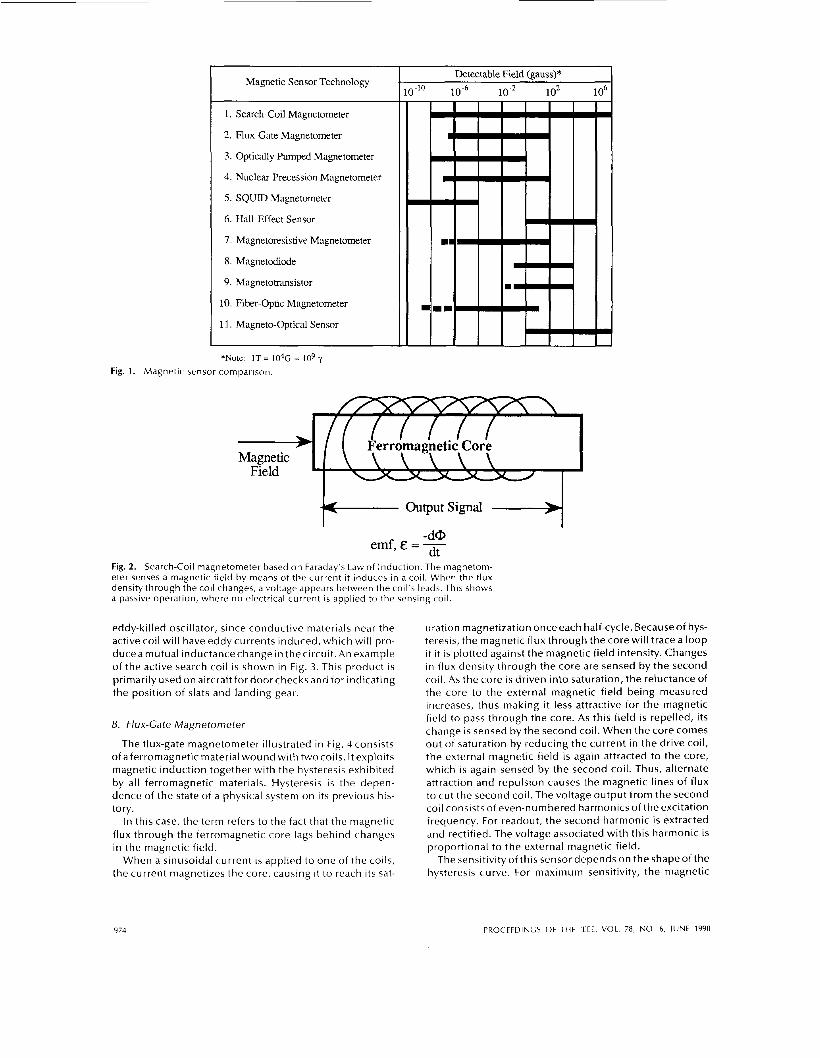
Magnetic sensing techniques exploit a broad range of physics and chemistry disciplines. Eleven of the more common magnetic sensor technologies are listed in Fig. 1, which compares approximate sensitivity ranges. In some cases, projected ranges based on further improvements are indi- cated by dashes. I t i s important to note that the sensitivity range for each concept is influenced by the readout electronics. There are many other factors, particularly frequency response, size, and power, that affect what sensor i s best suited for an application. A description of each of these concepts follows.

Manuscript received June 16, 1989. Theauthor iswith Systemsand Research Center, Honeywell, Inc.,

IEEE Log Number 9036163. 3660 Technology Drive, Minneapolis, MN 55418.

A. Search-Coil Magnetometer

The principle behind the search-coil magnetometer illustrated in Fig. 2 i s Faraday’s law of induction. If the magnetic flux through a coiled conductor changes, a current is induced in the coil and a voltage proportional to the rate of change of the flux is generated between its leads. The flux through the coil will change if the coil i s in a magnetic field that varies with time or if the coil i s moved through a nonuniform field. Typically, a rod of a ferromagnetic material with a high magnetic permeability i s inserted inside the coil to “gather” the surrounding magnetic field and increase flux density. (The permeability of a material is a measureof theextent to which i t modifies the magnetic flux through the region it occupies.)

The sensitivity of the search-coil magnetometer depends on the permeabilityof the core material, the area of the coil, the number of turns, and the rate of change of the magnetic flux through the coil. The frequency response of the sensor may be limited by the ratio of the coil’s inductance to its resistance, which determines the time i t takes the induced current to dissipate when the external magnetic field i s removed. The higher the inductance, the more slowly the current dissipates, and the lower the resistance, the more quickly it dissipates. In somecases, the interwindingcapac- itance can also l imit the frequency response. In practice, however, the voltage readout electronics can limit both the sensitivity and the frequency response of the sensor.

Sensors of this type can detect fields as weak as G, and there i s no upper l imit to their sensitivity range. Their useful frequency range i s typically from 1 Hz to 1 MHz, the upper l imit being that set by the ratio of the coil’s inductance to its resistance. The sensors can be as short as 2 in. or as long as 50 in. They require between 1 and 10 mW of power, all of which i s consumed in the readout electronics.

In addition to this passive use, one can also operate a search coil in an active mode. The active-mode method involves incorporating the search coil as an inductive element in an electrical circuit. There are two basic circuit designs. One incorporates a balanced inductive bridge where an inductance change in one leg of the bridge produces an out-of-balance voltage in the circuit. The second circuit design incorporates a resonant circuit where a change in inductance results in achange in the circuit’s resonant frequency. This circuit is sometimes referred to as an

0018-9219/90/0600-0973$01.00 0 1990 IEEE

PROCEEDINGS OF THE IEEE, VOL. 78, NO. 6, JUNE 1990 973

Magnetic Sensor Technology

1. Search-Coil Magnetometer

2. Flux-Gate Magnetometer

3. Optically Pumped Magnetometer

4. Nuclear-Precession Magnetometer

5. SQUID Magnetometer

6. Hal-Effect Sensor

7. Magnetoresistive Magnetometer

8. Magnetodiode

9. Magnetotransistor

10. Fiber-Optic Magnetometer

11. Magneto-Optical Sensor

*Note: 1T = 10% = IO9 y Fig. 1. Magnetic sensor comparison.

Detectable Field (gauss)*

Magneuc; Field I \ \ \ \ \ \

-d@ emf,&=- dt

Fig. 2 . Search-Coil magnetometer based on Faraday’s Law of Induction. The rnagnetom- eter senses a magnetic field by means of the current it induces in a coil. When the flux density through the coil changes, a voltage appears between the coil‘s leads. This shows a passive operation, where no electrical current i s applied to the sensing coil.

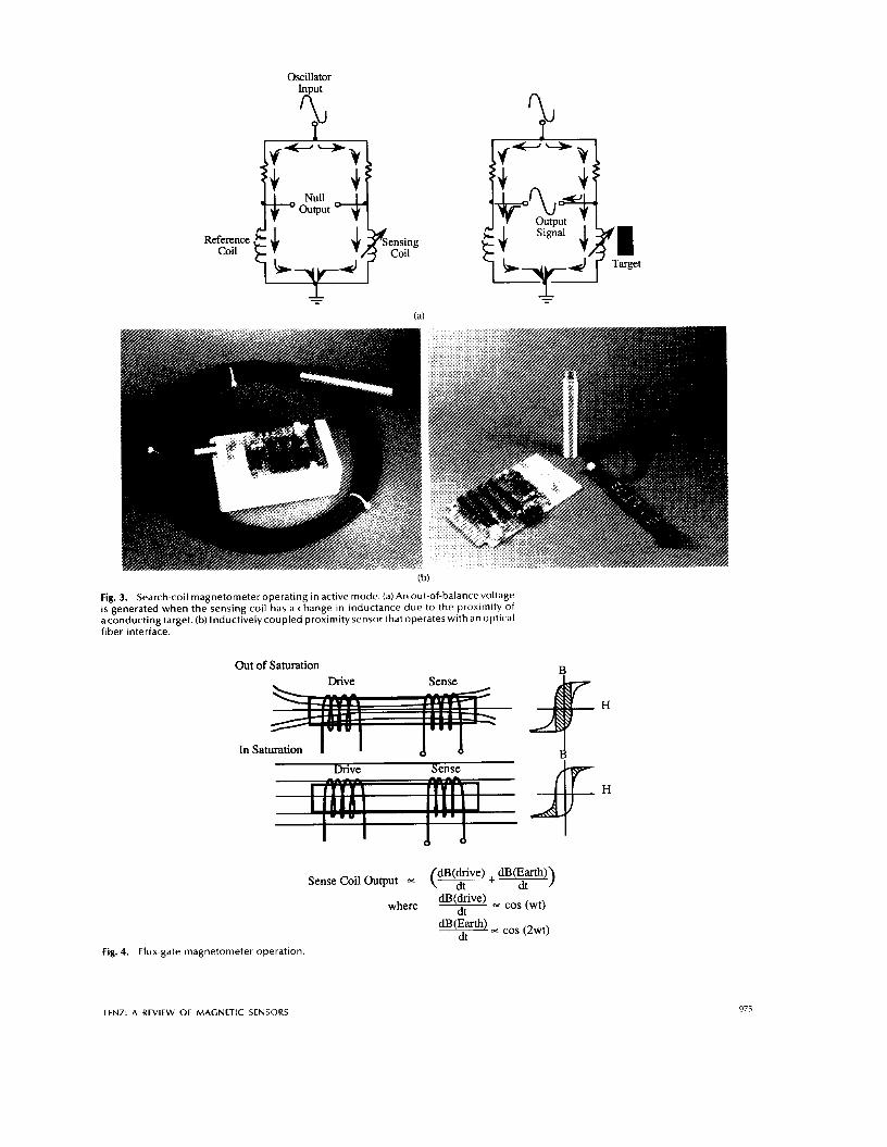
eddy-killed oscillator, since conductive materials near the active coil wil l have eddy currents induced, which wil l pro- duceamutual inductancechange in thecircuit.An example of the active search coil is shown in Fig. 3. This product i s primarily used on aircraft for door checks and for indicating the position of slats and landing gear.

B. Flux-Gate Magnetometer

The flux-gate magnetometer illustrated in Fig. 4 consists of aferromagnetic material wound with two coils. I t exploits magnetic induction together with the hysteresis exhibited by all ferromagnetic materials. Hysteresis is the depen- dence of the state of a physical system on its previous his- tory.

In this case, the term refers t o the fact that the magnetic flux through the ferromagnetic core lags behind changes in the magnetic field.

When a sinusoidal current i s applied to one of the coils, the current magnetizes the core, causing it to reach its sat-

uration magnetization once each half-cycle. Because of hysteresis, the magnetic flux through the core wil l trace a loop if i t i s plotted against the magnetic field intensity. Changes in flux density through the core are sensed by the second coil. As the core i s driven into saturation, the reluctance of the core to the external magnetic field being measured increases, thus making it less attractive for the magnetic field to pass through the core. As this field i s repelled, its change i s sensed by the second coil. When the core comes out of saturation by reducing the current in the drive coil, the external magnetic field is again attracted to the core, which is again sensed by the second coil. Thus, alternate attraction and repulsion causes the magnetic lines of flux to cut the second coil. The voltage output from the second coil consists of even-numbered harmonics of the excitation frequency. For readout, the second harmonic i s extracted and rectified. The voltage associated with this harmonic is proportional t o the external magnetic field.

The sensitivity of this sensor depends on the shapeof the hysteresis curve. For maximum sensitivity, the magnetic

974 PROCFFDINCS OF THE IEEE, VOL. 78, NO. 6, JUNE 1990

Oscillator

'L P

Sensing Reference coil 5 kTjf coil

(b)

Fig. 3. Search-coil magnetometer operating in active mode. (a) An out-of-balance voltage is generated when the sensing coil has a change in inductance due to the proximity of a conducting target. (b) Inductively coupled proximity sensor that operates with an optical fiber interface.

B Out of Saturation

H

In Sat

H

Fig. 4. Flux-gate magnetometer operation.

&(drive) &(Earth)) Sense coil Output = (7 + ____ dt

where =COS (wt)

LENZ: A REVIEW OF MAGNETIC SENSORS 975

field-magnetic induction (B-H) curve should be square, sincethis produces the highest induced electromotiveforce (emf) for a given value of Earth’s field. For minimum power consumption, the core material should have low coercivity and saturation values. The sensitivity range i s from G to 100 G. The frequency response of the sensor i s limited by the excitation field and the response time of the ferromagnetic material. The upper l imit on the frequency i s about 10 kHz. Flux-gate magnetometers resemble the search-coil magnetometers in size, but they consume roughly five times as much power. The major advantage of flux-gate magnetometers over search coils i s their ability to precisely measure direct current (dc) fields.

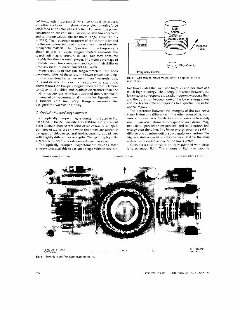
Many versions of flux-gate magnetometers have been developed. Most of these result in lower power consumption by operating the sensor on a minor hysteresis loop, thus not driving the core from saturation to saturation. These minor-loop flux-gate magnetometers are much more sensitive to the drive and readout electronics than the major-loop versions, which, as described above, are mostly dominated bythecore material‘s properties. Figure5 shows a toroidal core minor-loop flux-gate magnetometer designed for two-axis sensitivity.

C. Optically Pumped Magnetometer

The optically pumped magnetometer illustrated in Fig. 6 is based on theZeeman effect. In 1896 the Dutch physicist Peter Zeeman showed that some of the characteristic spectral lines of atoms are split when the atoms are placed in a magnetic field; one spectral line becomes a group of lines with slightly different wavelengths. The splitting i s particularly pronounced in alkali elements such as cesium.

The optically pumped magnetometer exploits three energy states available to cesium’s single valence electron:

Photodetector

Freauencv Control I Fig. 6. Optically pumped magnetometer exploits the Zee- man Effect.

two lower states that are close together and one state at a much higher energy. The energy difference between the lower states corresponds to a radio-frequency spectral line, and the transition between one of the lower energy states and the higher state corresponds to a spectral line in the optical region.

The difference between the energies of the two lower states i s due to a difference in the orientation of the spin axes of the electrons. An electron’s spin axis can have only one of two orientations with respect to an external magnetic field-parallel or antiparallel-and one requires less energy than the other. The lower energy states are said to differ in one quantum unit of spin angular momentum. The higher state is a special one chosen because it has the same angular momentum as one of the lower states.

Consider a cesium vapor optically pumped with circularly polarized light. The amount of light the vapor is

MAGNETIC AXIS FLYBACK OSCILLATOH I’OWEH SlJPPLY F I I TEN

* - 1 INCH _ _ - - PLAK DIFFER ENCF OCTECTOH I

Fig. 5. Toroidal core flux-gate magnetometer.

976 PROCEEDINGS OF THE IEEE, VOL. 78, NO. 6 , JUNE 1990

absorbing i s monitored with a photodetector. Initially, some of the electrons in the vapor wil l be in one of the lower energy states and some in the other. When atoms absorb photons from circularly polarized light, their angular momentum necessarily changes by one unit. Thus, electrons in the energy state that differs from the higher state by one unit of angular momentum will absorb photons and move to the higher state, but those in the energy state that

not. Because some photons are absorbed, the beam of light i s dimmed. An electron in the higher state drops down to

C

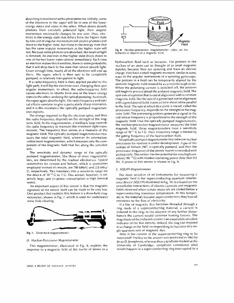
has the Same angular as the higher state will Fig. 8. Nuclear-precession magnetometer relies on the behavior of dipoles in a magnetic field,

one of the two lower states almost immediately. Each time an electron makes this transition, there is some probability that it will drop back to the state that cannot absorb light. Given enough time, nearly all of the electrons will end up there. The vapor, which i s then said to be completely pumped, is relatively transparent to light.

If a radio-frequency field i s then applied parallel to the light path, it wi l l flip the electrons over, changing their spin angular momentum. In effect, the radio-frequency field causes electrons to shuttle from one of the lower energy states to the other, undoing theoptical pumping. As a result, thevapor again absorbs light. The radiofrequencyand optical effects combine to give a particularly sharp resonance, and it is this resonance the optically pumped magnetometer exploits.

The energy required to flip the electron spins, and thus the radio frequency, depends on the strength of the magnetic field. In the magnetometer, a feedback loop controls the radio frequency to maintain the minimum light trans- mission. The frequency thus serves as a measure of the magnetic field. The optically pumped magnetometer measures the total magnetic field, whatever its orientation, unlike most magnetometers, which measure only the component of the magnetic field that lies along the sensitive axis.

The sensitivity and dynamic range of the optically pumped magnetometer, like those of most magnetometers, are determined by the readout electronics. Typical sensitivities for cesium and helium, which is sometimes employed instead of cesium, are 700 kHz/G and 2.8 MHz/ G, respectively. This translates into a sensitivity range for the device of G to 1 G. This sensor, however, i s relatively large, and its power consumption i s high (several watts).

An important aspect of this sensor i s that the magnetic signature of the sensor itself can be made to be very low. One product that exploits this feature i s a diver-held magnetometer, shown in Fig. 7, which is used for underwater mine field clearing.

Fig. 7. Diver-held magnetometer.

D. Nuclear-Precession Magnetometer

This magnetometer, illustrated in Fig. 8, exploits the response to a magnetic field of the nuclei of atoms in a

hydrocarbon fluid such as benzene. The protons in the nucleus of an atom can be thought of as small magnetic dipoles; because they are spinning and have an electric charge, they have a small magnetic moment, similar in some ways to the angular momentum of a spinning gyroscope. The protons in a fluid can be temporarily aligned by the uniform magnetic field created by a current through a coil. When the polarizing current i s switched off, the protons will begin to precess about the ambient magnetic field. The spin axis of a proton that i s out of alignment with a constant magnetic field, like the axis of a gyroscope out of alignment with a gravitational field, traces a circle about a line parallel to the field. The rate at which this circle is traced, called the precession frequency, depends on the strength of the magnetic field. The precessing protons generate a signal in the coil whose frequency is proportional t o the strength of the magnetic field. LI ke the optically pumped magnetometer, the nuclear-precession magnetometer measures the total magnetic field. These magnetometers have a sensitivity range of IO-’G to 1 G. Their frequency range i s limited by the gating frequency of the hydrocarbon fluid.

An optically pumped magnetometer that relies on nuclear precession for readout is under development. A gas of the isotope of helium, He3, is optically pumped, and then the precession frequency of the atomic nuclei i s recorded with pickupcoils. This sensor has the potential for very high sensitivity (10-8G) with modest operating power (less than 0.5 W). A photo of this sensor i s shown in Fig. 9.

E . SQUID Magnetometer

The most sensitive of all instruments for measuring a magnetic field i s the superconducting quantum interfer- encedevice(SQU1D) illustrated in Fig. I O . I t i s based on the remarkable interactions of electric currents and magnetic fields observed when certain materials are cooled below a superconducting transition temperature. At this temperature, the materials become superconductors; they lose all resistance to the flow of electricity.

If a line of magnetic flux becomes threaded through a ring made of a superconducting material, a current i s induced in the ring; in the absence of any further distur- bances the current would continue flowing forever. The magnitudeof the induced current is an exquisitelysensitive indicator of the flux density. Indeed, the ring can respond to a change in the field corresponding to fractions of a single quantum unit of magnetic flux.

How i s the current in the superconducting ring to be measured? The key to the answer was predicted in 1962 by Brian D. Josephson, who was then agraduate student at the University of Cambridge. Josephson considered what would happen in a superconducting ring interrupted by a


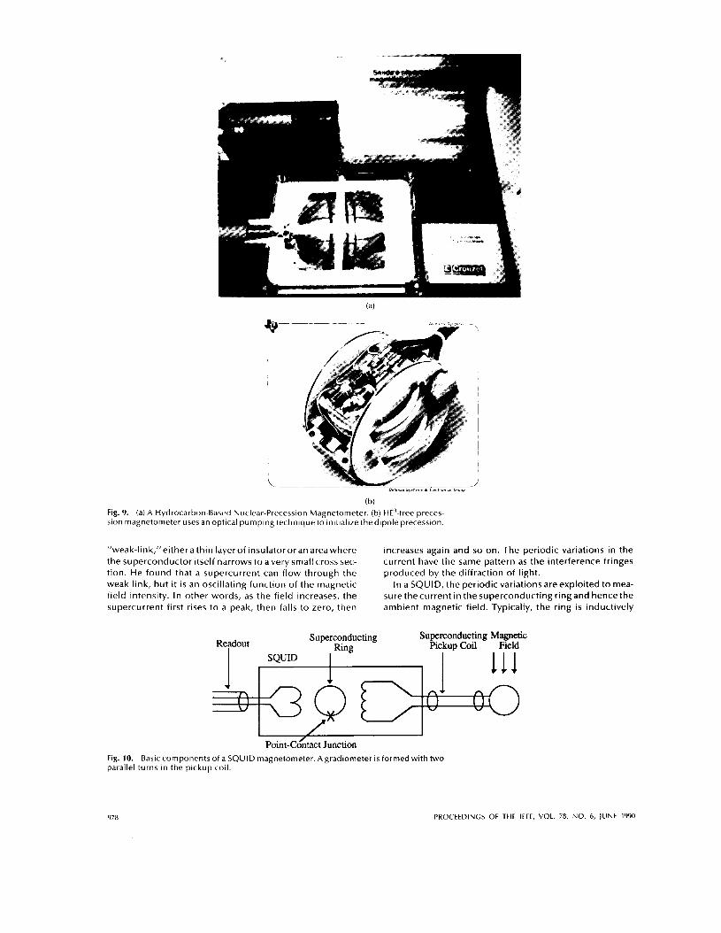
(b) Fig. 9. (a) A Hydrocarbon-Based Nuclear-Precession Magnetometer. (b) HE’-free precession magnetometer uses an optical pumping technique to initialize thedipole precession.

”weak-link,”either a thin layer of insulator or an areawhere the superconductor itself narrows to avery small cross section. He found that a supercurrent can flow through the weak link, but it i s an oscillating function of the magnetic field intensity. In other words, as the field increases, the supercurrent first rises to a peak, then falls to zero, then

increases again and so on. The periodic variations in the current have the same pattern as the interference fringes produced by the diffraction of light.

In a SQUID, the periodic variations are exploited to mea- surethecurrent in the superconducting ring and hencethe ambient magnetic field. Typically, the ring is inductively

Superconducting Superconducting Magnetic pickup Coil Field

I I

Ring Readout I S Q m

1 f ~ \ I I

Point- Contact Junction Fig. 10. parallel turns in the pickup coil.

Basic componentsof a SQUID magnetometer. Agradiometer i s formed with two

978 PROCEEDINGS OF THE IEEE, VOL. 78, NO. 6 , JUNE 1990

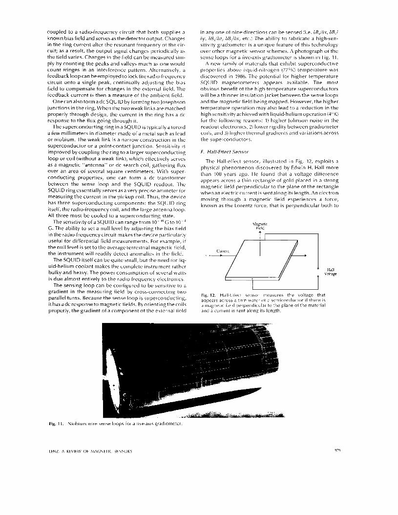
coupled to a radio-frequency circuit that both supplies a known bias field and serves as the detector output. Changes in the ring current alter the resonant frequency of the circuit; as a result, the output signal changes periodically as the field varies. Changes in the field can be measured sim- ply by counting the peaks and valleys much as one would count fringes in an interference pattern. Alternatively, a feedback loopcan beemployed to lockthe radio-frequency circuit onto a single peak, continually adjusting the bias field to compensate for changes in the external field. The feedback current i s then a measure of the ambient field.

Onecanalsoform adcSQUlD byformingtwo Josephson junctions in the ring. When thetwoweak linksare matched properly through design, the current in the ring has a dc response to the flux going through it.

The superconducting ring in a SQUID is typically a toroid a few millimeters in diameter made of a metal such as lead or niobium. The weak link i s a narrow construction in the superconductor or a point-contact junction. Sensitivity is improved by coupling the ring to a larger superconducting loop or coil (without a weak link), which effectively serves as a magnetic "antenna" or dc search coil, gathering flux over an area of several square centimeters. With superconducting properties, one can form a dc transformer between the sense loop and the SQUID readout. The SQUID ring essentially serves as a very precise ammeter for measuring the current in the pickup coil. Thus, the device has three superconducting components: the SQUID ring itself, the radio-frequency coil, and the large antenna loop. All three must be cooled to a superconducting state.

Thesensitivityof a SQUIDcan range from 10-" 'G to10-4 G. The ability to set a null level by adjusting the bias field in the radio-frequency circuit makes the device particularly useful for differential field measurements. For example, if the null level is set to the average terrestrial magnetic field, the instrument wil l readily detect anomalies in the field.

The SQUID itself can be quite small, but the need for liquid-helium coolant makes the complete instrument rather bulky and heavy. The power consumption of several watts i s due almost entirely to the radio-frequency electronics.

The sensing loop can be configured to be sensitive to a gradient in the measuring field by cross-connecting two parallel turns. Because the sense loop i s superconducting, it hasadc responseto magnetic fields. Byorientingthecoils properly, the gradient of a component of the external tield

in any one of nine directions can be sensed (i.e. GBJlix, 6B,l 6 y , GB,/6z, GBJlix, etc.) The ability to fabricate a high-sensitivity gradiometer is a unique feature of this technology over other magnetic sensor schemes. A photograph of the sense loops for a five-axis gradiometer is shown in Fig. 11.

A new family of materials that exhibit superconductive properties above liquid-nitrogen (77OK) temperature was discovered in 1986. The potential for higher temperature SQUID magnetometers appears available. The most obvious benefit of the high-temperature superconductors wil l be a thinner insulation jacket between the sense loops and the magnetic field being mapped. However, the higher temperature operation may also lead to a reduction in the high sensitivityachieved with liquid-helium operation ( 4 O K ) for the following reasons: 1) higher Johnson noise in the readout electronics, 2) lower rigidity between gradiometer coils, and 3) higher thermal gradients and variations across the superconductors.

F. Hall-Effect Sensoi

The Hall-effect sensor, illustrated in Fig. 12, exploits a physical phenomenon discovered by Edwin H. Hall more than 100 years ago. He found that a voltage difference appears across a thin rectangle of gold placed in a strong magnetic field perpendicular to the plane of the rectangle when an electric current is sent along its length. An electron moving through a magnetic field experiences a force, known as the Lorentz force, that i s perpendicular both to

Magnetic Field

I

Fig. 1 1 . Niobium wire sense loops for a five-axis gradiometer

LENZ: A REVIEW OF MACNtTIC S t N S O R S

Hall Voltage

Fig. 12. Hall-Efiect sensor mcasures the voltage that appears across a thin water o i a semiconductor if there is a magnetic tield p?rpendic-ular to t h e plane ot the material and a current is w n t along i t s length.

9 79

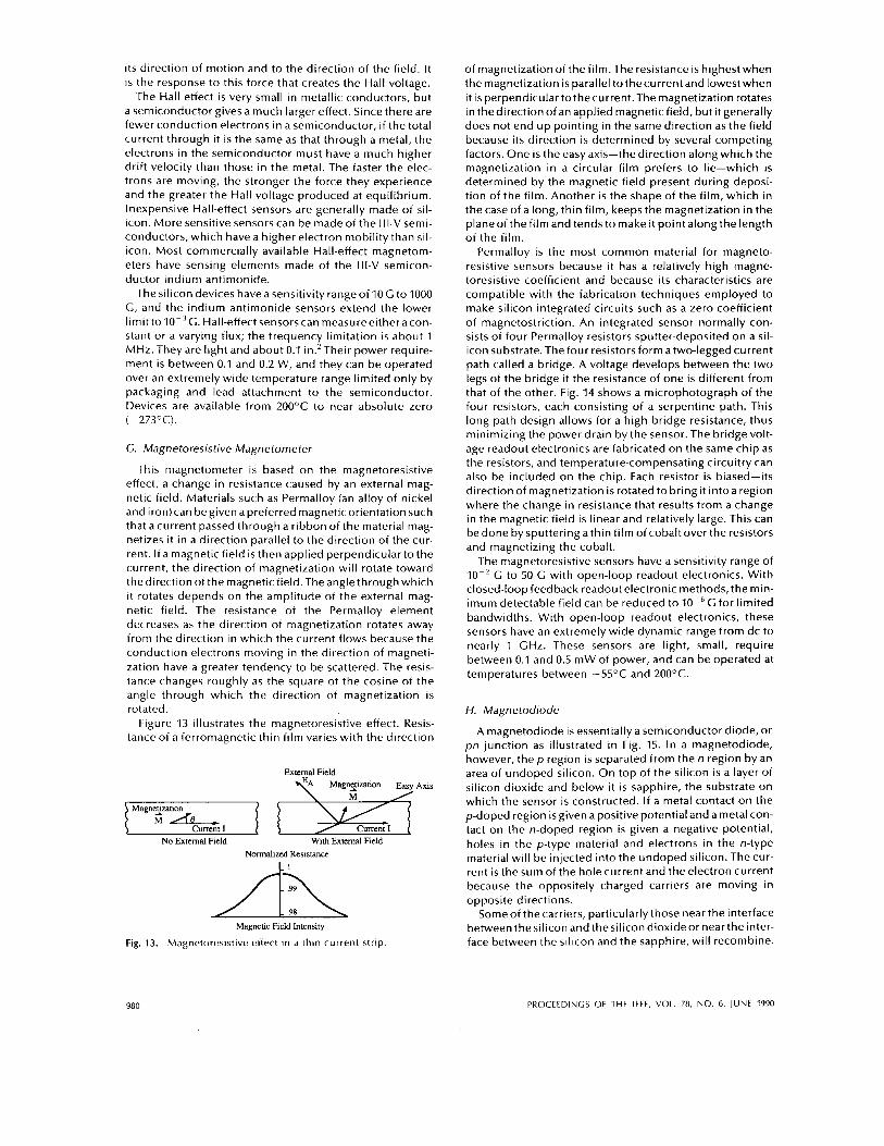
its direction of motion and to the direction of the field. It i s the response to this force that creates the Hall voltage.

The Hall effect i s very small in metallic conductors, but a semiconductor gives a much larger effect. Since there are fewer conduction electrons in a semiconductor, if the total current through it i s the same as that through a metal, the electrons in the semiconductor must have a much higher drift velocity than those in the metal. The faster the electrons are moving, the stronger the force they experience and the greater the Hall voltage produced at equilibrium. Inexpensive Hall-effect sensors are generally made of silicon. More sensitive sensors can be made of the l l I-V semi- conductors, which have a higher electron mobility than silicon. Most commercially available Hall-effect magnetometers have sensing elements made of the I l l -V semiconductor indium antimonide.

The silicon devices have a sensitivity range of 10 G to 1000 G, and the indium antimonide sensors extend the lower l imitto10-3G. Hall-effect sensorscan measureeitheracon- stant or a varying flux; the frequency limitation i s about 1 MHz. They are light and about 0.1 in.*Their power require- ment i s between 0.1 and 0.2 W, and they can be operated over an extremely wide temperature range limited only by packaging and lead attachment to the semiconductor. Devices are available from 2OOOC to near absolute zero (-273OC).

G. Magnetoresistive Magnetometer

This magnetometer is based on the magnetoresistive effect, a change in resistance caused by an external magnetic field. Materials such as Permalloy (an alloy of nickel and iron) can be given a preferred magnetic orientation such that a current passed through a ribbon of the material magnetizes it in a direction parallel to the direction of the current. If a magnetic field is then applied perpendicular to the current, the direction of magnetization will rotate toward the direction of the magnetic field. The angle through which it rotates depends on the amplitude of the external magnetic field. The resistance of the Permalloy element decreases as the direction of magnetization rotates away from the direction in which the current flows because the conduction electrons moving in the direction of magnetization have a greater tendency to be scattered. The resistance changes roughly as the square of the cosine of the angle through which the direction of magnetization i s rotated.

Figure 13 illustrates the magnetoresistive effect. Resis- tance of a ferromagnetic thin film varies with the direction

Magnetization PZJ rn No External Field With External Field

Normalized Resistance

Magnetic Field Intensity

Fig. 13. Magnetoresistive effect in a thin current strip

of magnetization of the film. The resistance is highestwhen the magnetization i s parallel to thecurrent and lowest when it is perpendicular to thecurrent. The magnetization rotates in thedirection of an applied magnetic field, but it generally does not end up pointing in the same direction as the field because its direction i s determined by several competing factors. One i s the easy axis-the direction along which the magnetization in a circular f i lm prefers to lie-which i s determined by the magnetic field present during deposi- tion of the film. Another i s the shape of the film, which in the case of a long, thin film, keeps the magnetization in the planeof the fi lm and tends to make it point along the length of the film.

Permalloy is the most common material for magnetoresistive sensors because it has a relatively high magnetoresistive coefficient and because its characteristics are compatible with the fabrication techniques employed to make silicon integrated circuits such as a zero coefficient of magnetostriction. An integrated sensor normally consists of four Permalloy resistors sputter-deposited on a silicon substrate. The four resistors form a two-legged current path called a bridge. A voltage develops between the two legs of the bridge if the resistance of one i s different from that of the other. Fig. 14 shows a microphotograph of the four resistors, each consisting of a serpentine path. This long path design allows for a high bridge resistance, thus minimizing the power drain by the sensor. The bridge voltage readout electronics are fabricated on the same chip as the resistors, and temperature-compensating circuitry can also be included on the chip. Each resistor i s biased-its direction of magnetization i s rotated to bring it intoa region where the change in resistance that results from a change in the magnetic field is linear and relatively large. This can bedone by sputteringathin film of cobaltoverthe resistors and magnetizing the cobalt.

The magnetoresistive sensors have a sensitivity range of IO-’ G to 50 G with open-loop readout electronics. With closed-loop feedback readout electronic methods, the minimum detectable field can be reduced to G for limited bandwidths. With open-loop readout electronics, these sensors have an extremely wide dynamic range from dc to nearly 1 GHz. These sensors are light, small, require between 0.1 and 0.5 mW of power, and can be operated at temperatures between -55OC and 200°C.

H. Magnetodiode

A magnetodiode is essentially a semiconductor diode, or pn junction as illustrated in Fig. 15. In a magnetodiode, however, the p region is separated from the n region by an area of undoped silicon. O n top of the silicon i s a layer of silicon dioxide and below it is sapphire, the substrate on which the sensor i s constructed. If a metal contact on the p-doped region is given a positive potential and a metal contact on the n-doped region i s given a negative potential, holes in the p-type material and electrons in the n-type material will be injected into the undoped silicon. The current is the sum of the hole current and the electron current because the oppositely charged carriers are moving in opposite directions.

Some of the carriers, particularly those near the interface between thesilicon and thesilicon dioxideor nearthe interface between the silicon and the sapphire, will recombine.

980 PROCEEDINGS OF THE IEEE, VOL. 78, NO. 6, JUNE 1990

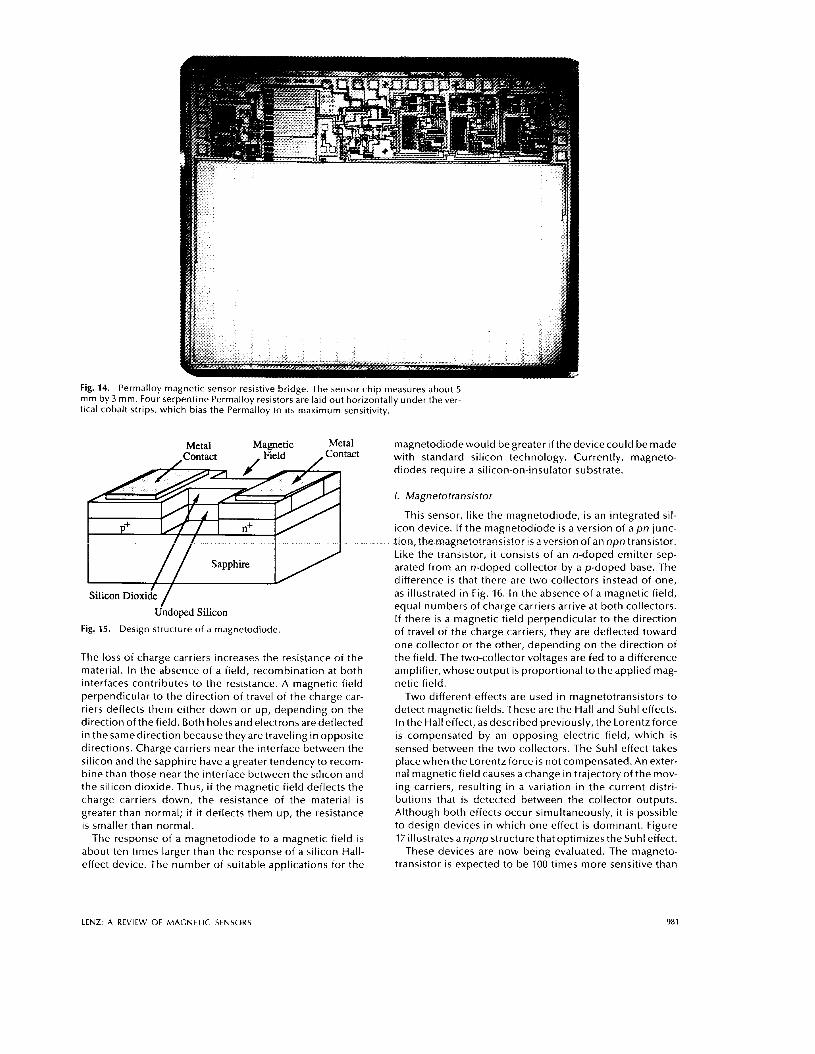
Fig. 14. Permalloy magnetic sensor resistive bridge. The sensor chip measures about 5 mm by 3 mm. Four serpentine Permalloy resistors are laid out horizontally under the vertical cobalt strips, which bias the Permalloy to i t s maximum sensitivity.

Metal Magnetic Metal .Contact I Field , Contact

Sapphire

/ Silicon Dioxiie Undoped Silicon

Fig. 15. Design structure of a magnetodiode.

The loss of charge carriers increases the resistance of the material. In the absence of a field, recombination at both interfaces contributes to the resistance. A magnetic field perpendicular to the direction of travel of the charge carriers deflects them either down or up, depending on the direction of the field. Both holes and electrons are deflected in the samedirection because they are traveling in opposite directions. Charge carriers near the interface between the silicon and the sapphire have a greater tendency to recombine than those near the interface between the silicon and the silicon dioxide. Thus, if the magnetic field deflects the charge carriers down, the resistance of the material is greater than normal; if it deflects them up, the resistance is smaller than normal.

The response of a magnetodiode to a magnetic field is about ten times larger than the response of a silicon Hall- effect device. The number of suitable applications for the

magnetodiode would be greater if the device could be made with standard silicon technology. Currently, magneto- diodes require a silicon-on-insulator substrate.

1. Magnetotransistor

This sensor, like the magnetodiode, i s an integrated silicon device. If the magnetodiode i s a version of a pn junction, the magnetotransistor is aversion of an npn transistor. Like the transistor, it consists of an n-doped emitter separated from an n-doped collector by a p-doped base. The difference i s that there are two collectors instead of one, as illustrated in Fig. 16. In the absence of a magnetic field, equal numbers of charge carriers arrive at both collectors. If there is a magnetic field perpendicular to the direction of travel of the charge carriers, they are deflected toward one collector or the other, depending on the direction of the field. The two-collector voltages are fed to a difference amplifier, whose output is proportional to the applied magnetic field.

Two different effects are used in magnetotransistors to detect magnetic fields. These are the Hall and Suhl effects. In the Hall effect, as described previously, the Lorentzforce is compensated by an opposing electric field, which i s sensed between the two collectors. The Suhl effect takes place when the Lorentz force i s not compensated. An external magnetic field causes a change in trajectory of the moving carriers, resulting in a variation in the current distri- butions that i s detected between the collector outputs. Although both effects occur simultaneously, it i s possible to design devices in which one effect is dominant. Figure 17 illustrates a npnp structure that optimizes the Suhl effect.

These devices are now being evaluated. The magnetotransistor i s expected to be 100 times more sensitive than


A Base :tic / A

Difference Amplifier

Left Collector r

0 Right

Base Collector

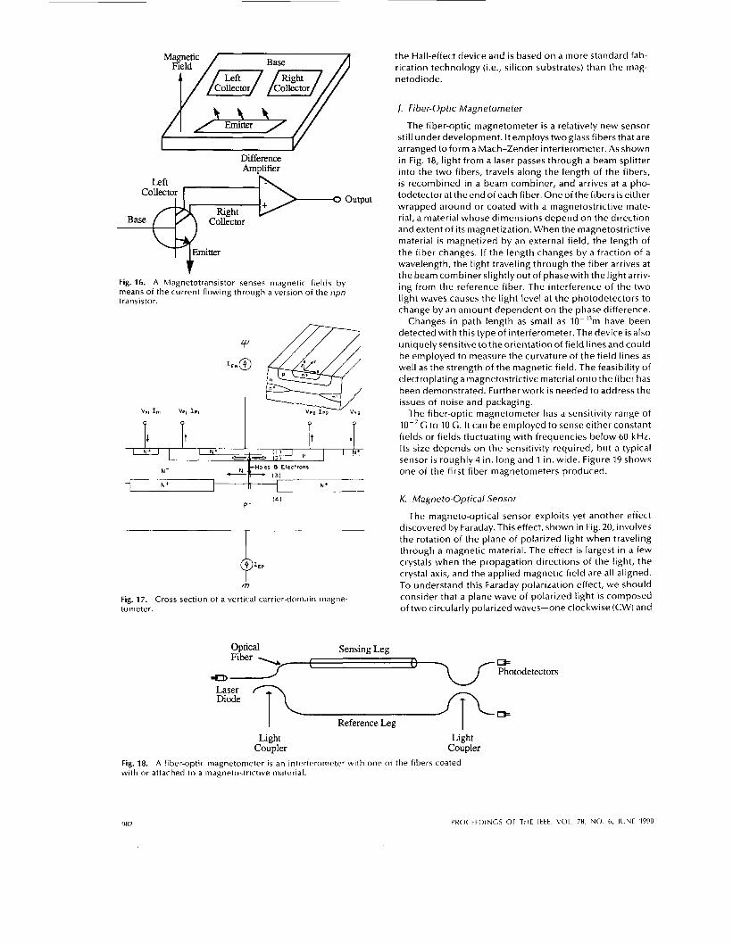
‘ t Fig. 16. A Magnetotransistor senses magnetic fields by means of the current flowing through a version of the npn transistor.

output

o... d7

Fig. 17. Cross section of a vertical carrier-domain magnetometer.

the Hall-effect device and i s based on a more standard fabrication technology (i.e., silicon substrates) than the magnetodiode.

1. Fiber-optic Magnetometer

The fiber-optic magnetometer i s a relatively new sensor still under development. It employs two glass fibers that are arranged to form a Mach-Zender interferometer. As shown in Fig. 18, light from a laser passes through a beam splitter into the two fibers, travels along the length of the fibers, i s recombined in a beam combiner, and arrives at a photodetector at the end of each fiber. One of the fibers is either wrapped around or coated with a magnetostrictive material, a material whose dimensions depend on the direction and extent of its magnetization. When the magnetostrictive material is magnetized by an external field, the length of the fiber changes. If the length changes by a fraction of a wavelength, the light traveling through the fiber arrives at the beam combiner slightlyout of phasewith the light arriv- ing from the reference fiber. The interference of the two light waves causes the light level at the photodetectors to change by an amount dependent on the phase difference.

Changes in path length as small as IO-l3m have been detected with this type of interferometer. The device i s also uniquely sensitive to the orientation of field lines and could be employed to measure the curvature of the field lines as well as the strength of the magnetic field. The feasibility of electroplating a magnetostrictive material onto the fiber has been demonstrated. Further work i s needed to address the issues of noise and packaging.

The fiber-optic magnetometer has a sensitivity range of IO-’G to 10 G. I t can be employed to sense either constant fields or fields fluctuating with frequencies below 60 kHz. Its size depends on the sensitivity required, but a typical sensor i s roughly 4 in. long and 1 in. wide. Figure 19 shows one of the first fiber magnetometers produced.

K. Magneto-Optical Sensor

The magneto-optical sensor exploits yet another effect discovered by Faraday. This effect, shown in Fig. 20, involves the rotation of the plane of polarized light when traveling through a magnetic material. The effect is largest in a few crystals when the propagation directions of the light, the crystal axis, and the applied magnetic field are all aligned. To understand this Faraday polarization effect, we should consider that a plane wave of polarized light i s composed of two circularly polarized waves-one clockwise (CW) and

Optical Sensing Leg I f i \ U m

Photodetectors =ED

I Reference Leg I Light

Coupler Light

Coupler Fig. 18. A fiber-optic magnetometer is an interferometer with one of the fibers coated with or attached to a magnetostrictive material.

982 PKOCttDlNCS OF THE IEEE. VOL. 7 8 , NO. 6 , JUNE 1990

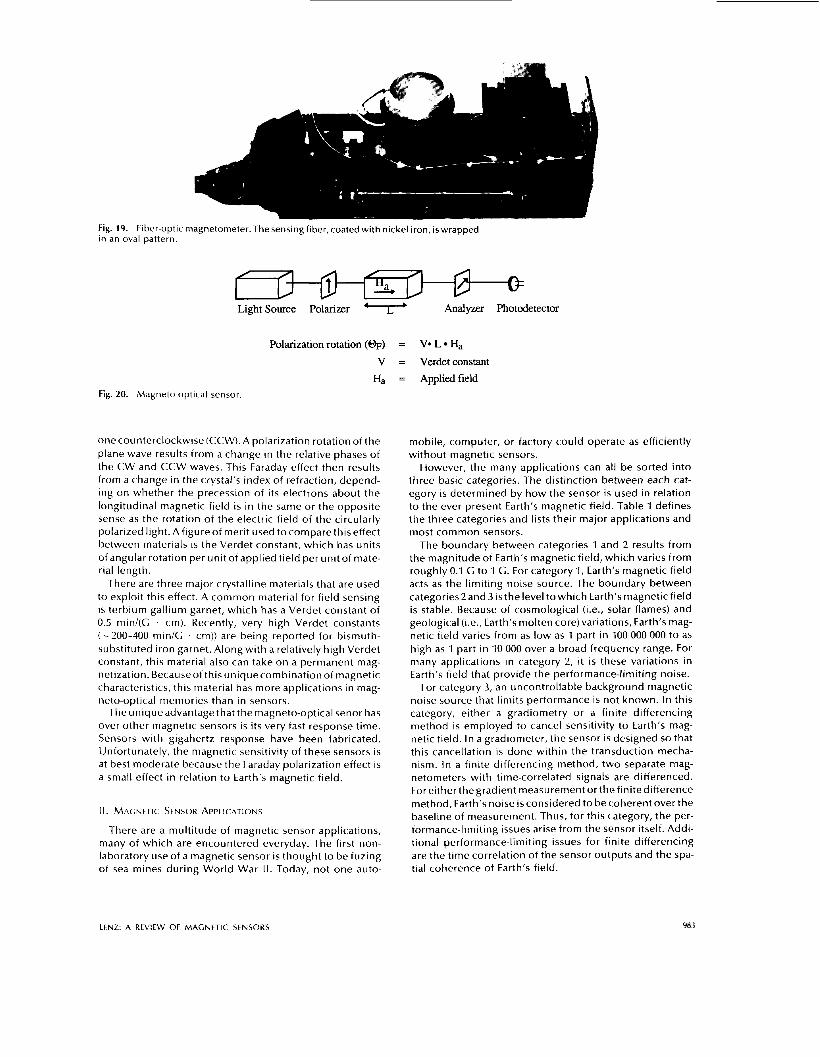
Fig. 19. Fiber-optic magnetometer. The sensing fiber, coated with nickel iron, iswrapped in an oval pattern.

Light Source Polarizer ‘7’ Analyzer Photodetector

Polarization rotation ( 0 ~ ) = V* L Ha

V = Verdetconstant = Applidfield

Fig. 20. Magneto-optical sensor.

one counterclockwise (CCW). A polarization rotation of the plane wave results from a change in the relative phases of the CW and CCW waves. This Faraday effect then results from a change in the crystal’s index of refraction, depending on whether the precession of its electrons about the longitudinal magnetic field i s in the same or the opposite sense as the rotation of the electric field of the circularly polarized light. Afigure of merit used tocomparethis effect between materials i s the Verdet constant, which has units of angular rotation per unit of applied field per unit of material length.

There are three major crystalline materials that are used to exploit this effect. A common material for field sensing i s terbium gallium garnet, which has a Verdet constant of 0.5 min/(G . cm). Recently, very high Verdet constants (-200-400 min/G . cm)) are being reported for bismuth- substituted iron garnet. Along with a relatively high Verdet constant, this material also can take on a permanent magnetization. Because of this uniquecombination of magnetic characteristics, this material has more applications in magneto-optical memories than in sensors.

The unique advantage that the magneto-optical senor has over other magnetic sensors is its very fast response time. Sensors with gigahertz response have been fabricated. Unfortunately, the magnetic sensitivity of these sensors i s at best moderate because the Faraday polarization effect i s a small effect in relation to Earth’s magnetic field.

II. MAGNETIC SENSOR APPLICATIONS

There are a multitude of magnetic sensor applications, many of which are encountered everyday. The first non- laboratory use of a magnetic sensor i s thought to be fuzing of sea mines during World War II. Today, not one auto-

mobile, computer, or factory could operate as efficiently without magnetic sensors.

However, the many applications can all be sorted into three basic categories. The distinction between each category i s determined by how the sensor i s used in relation to the ever present Earth’s magnetic field. Table 1 defines the three categories and lists their major applications and most common sensors.

The boundary between categories 1 and 2 results from the magnitude of Earth‘s magnetic field, which varies from roughly 0.1 G to 1 G. For category 1, Earth’s magnetic field acts as the l imiting noise source. The boundary between categories2 and 3 i s the level to which Earth’s magnetic field i s stable. Because of cosmological (i.e., solar flames) and geological (i.e., Earth’s molten core) variations, Earth’s magnetic field varies from as low as 1 part in 100 000 000 to as high as 1 part in 10 000 over a broad frequency range. For many applications in category 2, it is these variations in Earth’s field that provide the performance-limiting noise.

For category 3, an uncontrollable background magnetic noise source that limits performance i s not known. In this category, either a gradiometry or a finite differencing method is employed to cancel sensitivity to Earth’s magnetic field. In a gradiometer, the sensor i s designed so that this cancellation i s done within the transduction mechanism. In a finite differencing method, two separate magnetometers with time-correlated signals are differenced. For either thegradient measurement or the finite difference method, Earth’s noise i s considered to be coherent over the baseline of measurement. Thus, for this category, the performance-limiting issues arise from the sensor itself. Addi- tional performance-limiting issues for finite differencing are the time correlation of the sensor outputs and the spa- tial coherence of Earth‘s field.


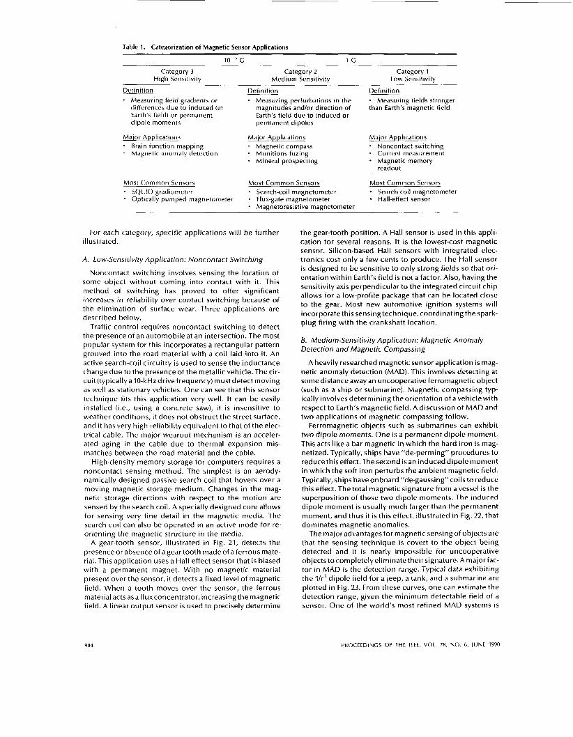
Table 1. Categorization of Magnetic Sensor Applications

IO-^ c I C

Category 3 High Sensitivity

Category 2 Medium Sensitivitv

Category 1 Low Sensitivity

Definition Measuring field gradients or differences due to induced (in Earth’s field) or permanent dipole moments

Major Applications * Brain function mapping * Magnetic anomaly detection

Most Common Sensors * SQUID gradiometer * Optically pumped magnetometer

Definition * Measuring perturbations in the

magnitudes and/or direction of Earth‘s field due to induced or permanent dipoles

Major Applications Magnetic compass

* Munitions fuzing - Mineral prospecting

Most Common Sensors * Search-coil magnetometer * Flux-gate magnetometer - Magnetoresistive magnetometer

Definition * Measuring fields stronger than Earth’s magnetic field

Major Applications - Noncontact switching * Current measurement * Magnetic memory

readout

Most Common Sensors Search-coil magnetometer Hall-effect sensor

For each category, specific applications will be further illustrated.

A. Low-Sensitivity Application: Noncontact Switching

Noncontact switching involves sensing the location of some object without coming into contact with it. This method of switching has proved to offer significant increases in reliability over contact switching because of the elimination of surface wear. Three applications are described below.

Traffic control requires noncontact switching to detect the presence of an automobile at an intersection. The most popular system for this incorporates a rectangular pattern grooved into the road material with a coil laid into it. An active search-coil circuitry i s used to sense the inductance change due to the presence of the metallic vehicle. The circu it (typically a 10-kHz d rive f req uency) mu st detect moving as well as stationary vehicles. One can see that this sensor technique fits this application very well. I t can be easily installed (i.e., using a concrete saw), it i s insensitive to weather conditions, it does not obstruct the street surface, and it has very high reliability equivalent to that of the electrical cable. The major wearout mechanism i s an acceler- ated aging in the cable due to thermal expansion mis- matches between the road material and the cable.

High-density memory storage for computers requires a noncontact sensing method. The simplest i s an aerody- namically designed passive search coil that hovers over a moving magnetic storage medium. Changes in the magnetic storage directions with respect to the motion are sensed by the search coil. A specially designed core allows for sensing very fine detail in the magnetic media. The search coil can also be operated in an active mode for re- orienting the magnetic structure in the media.

A gear-tooth sensor, illustrated in Fig. 21, detects the presence or absence of a gear tooth made of a ferrous material. This application uses a Hall-effect sensor that is biased with a permanent magnet. With no magnetic material present over the sensor, i t detects a fixed level of magnetic field. When a tooth moves over the sensor, the ferrous material acts as afluxconcentrator, increasing the magnetic field. A linear output sensor i s used to precisely determine

the gear-tooth position. A Hall sensor i s used in this application for several reasons. I t is the lowest-cost magnetic sensor. Silicon-based Hall sensors with integrated electronics cost only a few cents to produce. The Hall sensor i s designed to be sensitive to only strong fields so that orientation within Earth’s field i s not a factor. Also, having the sensitivity axis perpendicular to the integrated circuit chip allows for a low-profile package that can be located close to the gear. Most new automotive ignition systems will incorporate this sensing technique, coordinating the spark- plug firing with the crankshaft location.

B. Medium-Sensitivity Application: Magnetic Anomaly Detection and Magnetic Compassing

A heavily researched magnetic sensor application i s magnetic anomaly detection (MAD). This involves detecting at some distance away an uncooperative ferromagnetic object (such as a ship or submarine). Magnetic compassing typically involves determining the orientation of a vehicle with respect to Earth’s magnetic field. A discussion of MAD and two applications of magnetic compassing follow.

Ferromagnetic objects such as submarines can exhibit two dipole moments. One is a permanent dipole moment. This acts like a bar magnetic in which the hard iron i s magnetized. Typically, ships have ”de-perming” procedures to reducethiseffect.Thesecond isan induced dipole moment in which the soft iron perturbs the ambient magnetic field. Typically, ships have onboard “de-gaussing” coils to reduce this effect. The total magnetic signature from a vessel i s the superposition of these two dipole moments. The induced dipole moment i s usually much larger than the permanent moment, and thus it i s this effect, illustrated in Fig. 22, that dominates magnetic anomalies.

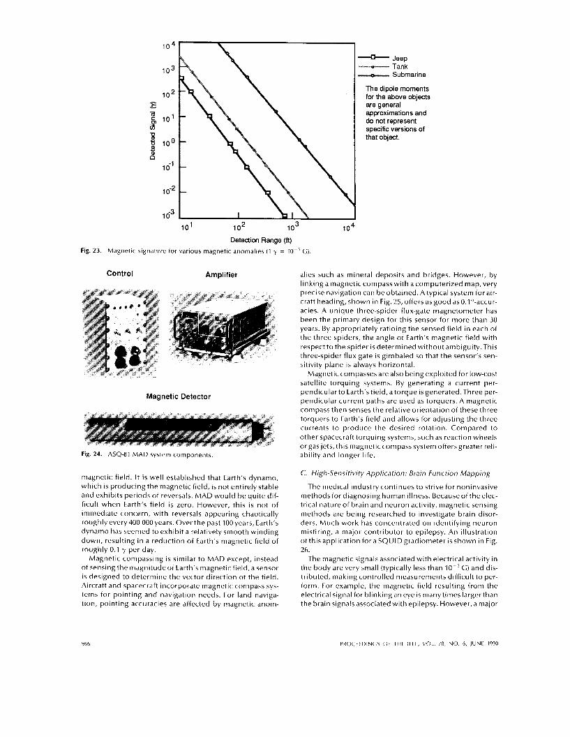
The major advantages for magnetic sensing of objects are that the sensing technique i s covert to the object being detected and i t i s nearly impossible for uncooperative objects tocompletelyeliminate their signature. A major factor in MAD is the detection range. Typical data exhibiting the l / r3 dipole field for a jeep, a tank, and a submarine are plotted in Fig. 23. From these curves, one can estimate the detection range, given the minimum detectable field of a sensor. One of the world’s most refined MAD systems i s

984 PROCEEDINGS OF THE IEEE, VOL. 78. NO. 6, JUNE 1990

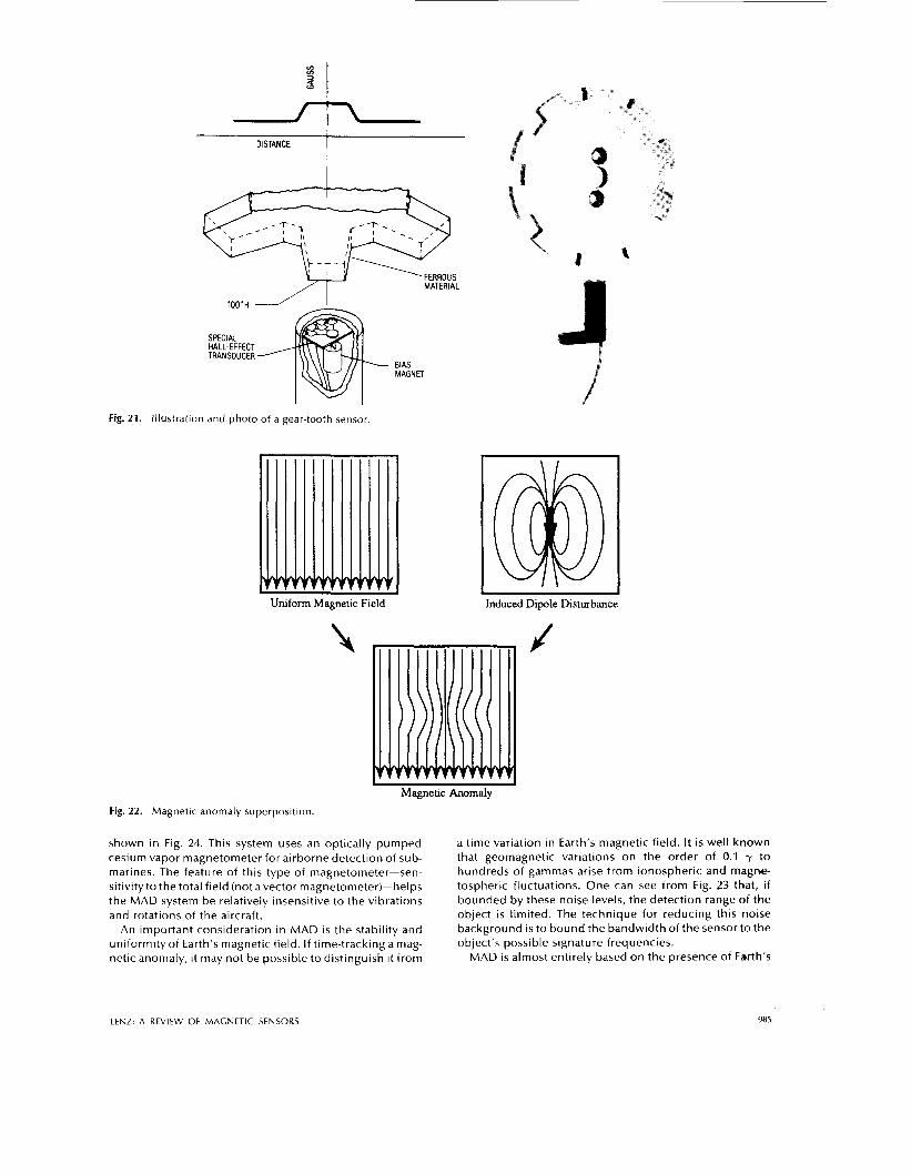
I DISTANCE

MATERIAL

TOOTH

Fig. 21. Illustration and photo of a gear-tooth sensor.

Uniform Magnetic Field Induced Dipole Disturbance

Magnetic Anomaly Fig. 22. Magnetic anomaly superposition.

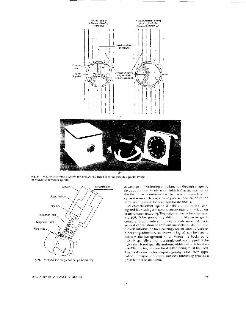
shown in Fig. 24. This system uses an optically pumped cesium vapor magnetometer for airborne detection of submarines. The feature of this type of magnetometer-sensitivity to the total field (not avector magnetometer)-helps the MAD system be relatively insensitive to the vibrations and rotations of the aircraft.

An important consideration in MAD i s the stability and uniformity of Earth’s magnetic field. If time-tracking a magnetic anomaly, it may not be possible to distinguish it from

a time variation in Earth’s magnetic field. I t i s well known that geomagnetic variations on the order of 0.1 y to hundreds of gammas arise from ionospheric and magne- tospheric fluctuations. One can see from Fig. 23 that, if bounded by these noise levels, the detection range of the object is limited. The technique for reducing this noise background i s to bound the bandwidth of the sensor to the object’s possible signature frequencies.

MAD is almost entirely based on the presence of Earth’s


101 102 10’ Detection Range (ft)

Fig. 23. Magnetic signature for various magnetic anomalies (1 y = IO-’ C).

Control Amp1 if ier

Magnetic Detector

Fig. 24. ASQ-81 MAD system components

magnetic field. It i s well established that Earth’s dynamo, which is producing the magnetic field, i s not entirely stable and exhibits periods of reversals. MAD would be quite difficult when Earth’s field is zero. However, this i s not of immediate concern, with reversals appearing chaotically roughly every400 000 years. Over the past 100 years, Earth’s dynamo has seemed to exhibit a relatively smooth winding down, resulting in a reduction of Earth‘s magnetic field of roughly 0.1 y per day.

Magnetic compassing i s similar to MAD except, instead of sensing the magnitude of Earth‘s magnetic field, a sensor i s designed to determine the vector direction of the field. Aircraft and spacecraft incorporate magnetic compass systems for pointing and navigation needs. For land navigation, pointing accuracies are affected by magnetic anom-

e Jeep - Tank --o.-- Submarine

The dipole moments for the above objects are general approximations and do not represent specific versions of that object.

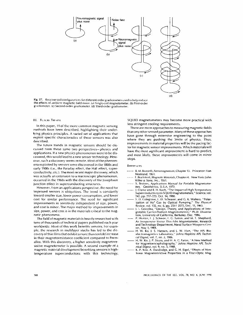
alies such as mineral deposits and bridges. However, by linking a magnetic compass with a computerized map, very precise navigation can be obtained. A typical system for aircraft heading, shown in Fig. 25, offers as good as O.lo-accuracies. A unique three-spider flux-gate magnetometer has been the primary design for this sensor for more than 30 years. By appropriately ratioing the sensed field in each of the three spiders, the angle of Earth’s magnetic field with respect to the spider is determined without ambiguity. This three-spider flux gate i s gimbaled so that the sensor’s sensitivity plane is always horizontal.

Magnetic compasses are also being exploited for low-cost satellite torquing systems. By generating a current perpendicular to Earth‘s field, a torque is generated. Three perpendicular current paths are used as torquers. A magnetic compass then senses the relative orientation of these three torquers to Earth‘s field and allows for adjusting the three currents to produce the desired rotation. Compared to other spacecraft torquing systems, such as reaction wheels or gas jets, this magnetic compass system offers greater reliability and longer life.

C. High-Sensitivity Application: Brain Function Mapping

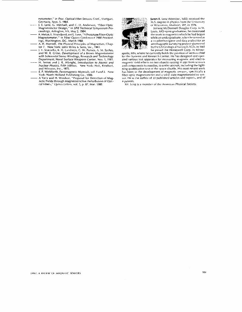
The medical industry continues to strive for noninvasive methods for diagnosing human illness. Because of the electrical nature of brain and neuron activity, magnetic sensing methods are being researched to investigate brain disor- ders. Much work has concentrated on identifying neuron misfiring, a major contributor to epilepsy. An illustration of this application for a SQUID gradiometer is shown in Fig. 26.

The magnetic signals associated with electrical activity in the body are very small (typically less than G) and dis- tributed, making controlled measurements difficult to per- form. For example, the magnetic field resulting from the electrical signal for blinking an eye i s manytimes largerthan the brain signals associated with epilepsy. However, a major

986 PKOCEEDINCS OF THE IEEE, VOL. 78, NO. 6, JUNE 1990

AircraH Flying at a Constant Heading

(northerly)

AircraH Changes Heading (go" to right) Spider

Rotates in Azimuth 90"

Collector - Horn

%der (lop view)

Fig. 25. Magnetic compass system for aircraft. (a). Three-arm flux-gate design. (b). Photo ofrnagnetic;ompass system.'

Dewar

To electronics

Liquid helium

SQUID

Detection coil. / A d Magnetic field \x$

Field map, n A JJ

Fig. 26. Method for magnetoencephalography.

LENZ: A REVIEW OF MAGNETIC SENSORS

advantage of monitoring body function through magnetic fields as opposed to electrical fields i s that the position of the field lines i s uninfluenced by tissue surrounding the current source. Hence, a more precise localization of the stimulus origin can be obtained for diagnosis.

Much of the effort expended in this application i s design- ing and fabricating a magnetic sensor that i s optimized for brain function mapping.The major sensortechnology used i s a SQUID because of the ability to build precise gradiometers. Gradiometers not only provide excellent background cancellation of ambient magnetic fields, but also provide information for localizing current sources. Various orders of gradiometry, as shown in Fig. 27, can be used to subtract the background noise. When the background noise i s spatially uniform, a single coil pair is used. If the noise field i s not spatially uniform, additional coils for dou- ble-differencing or even third-differencing must be used. This field of magnetoencephalography i s the latest application of magnetic sensors and may ultimately provide a great benefit to mankind.

987

Neuromagnetic plus noise

(a)

signal I I Noise field I I

plus noise

Fig. 27. Receiver coil configurations for different ordergradiometers used to help reduce the effects of ambient magnetic field noise. (a) Single-coil magnetometer. (b) First-order gradiometer. (c) Second-order gradiometer. (d) Third-order gradiometer.

Ill. FUTURE TRENDS

In this paper, 11 o f the more common magnetic sensing methods have been described, highlighting their under- tying physics principles. A varied set of applications that exploit specific characteristics of these sensors was also described.

The future trends in magnetic sensors should be discussed from these same two perspectives-physics and applications. If a new physics phenomenon were to be discovered, this would lead to a new sensor technology. How- ever, such a discovery seems remote. Most o f the phenomena exploited by sensors were discovered in the 1800s and early 1900s (i.e., the Faraday effect, the Hall effect, superconductivity, etc.). The most recent major discovery, which was actually an extension to a macroscopic phenomenon, occurred in the 1960s with the discovery of the Josephson junction effect in superconducting structures.

However, from an applications perspective, the need for improved sensors is ubiquitous. The trend is constantly toward smaller size, lower power consumption, and lower cost for similar performance. The need for significant improvements in sensitivity independent o f size, power, and cost i s minor. The major method for improvements in size, power, and cost is in the materials critical to the magnetic phenomena.

The field of magnetic materials i s heavily researched with tens of thousands of technical papers published each year worldwide. Most of this work benefits sensors. For example, the research in multilayer stacks has led to the discovery of thin films that exhibit a more than tenfold increase in their magnetoresistance coefficient compared to Perm- alloy. With this discovery, a higher sensitivity magnetoresistive magnetometer i s possible. A second example o f a magnetic material development benefiting sensors is high- temperature superconductors: with this technology,

SQUID magnetometers may become more practical with less stringent cooling requirements.

There are more approaches to measuring magnetic fields than any other sensed parameter. Many of theseapproaches have gone through extensive engineering to the point where they are pushing the limits of physics. Thus, improvements in material properties will be the pacing factor for magnetic sensor improvements. Which materials will have the most significant improvement is hard to predict, and most likely, these improvements will come in minor steps.

REFERENCES

- R. M. Bozorth, Ferromagnetism, Chapter 13. Princeton: Van

- F. Brailsford, MagneticMaterials, Chapter4. New York: John Nostrand, 1951.

Wiley & Sons, Inc., 1951. S. Breiner, Applications Manual for Portable Magnetome- ters. CeoMetrics, U.S.A. 1973. I. Clarke and R. H. Koch, ”The Impact of High Temperature Superconductivity on SQUID Magnetometers,” Science, vol.

F. D. Colegrove, L. D. Schearer, and G. K. Walters, “Polar- ization of He3 Gas by Optical Pumping,” The Physical Review, vol. 132, no. 6, pp. 2561-2572, Dec. 15, 1963. I . I. Coicolea, ”Design, Theory, and Applications of Inte- gratable Carrier-Domain Magnetometers,” Ph.D. Disserta- tion, University of California, Berkeley, Dec. 1986. P. Hunter, L. j. Schwee, F. G. Salton, and M. T. Shephard, An Inexpensive Vector Thin film Magnetometer, Research and Technology Department, Naval Surface Weapons Cen- ter, May 1, 1984. H. W. KO, J. S. Hansen, and L. W. Hart, “The APL Bio- electromagnetics Laboratory,” johns Hopkins APL Techni- cal Digest, vol. 7, no. 3, 1986. H. W. KO, J. P. Skura, and H. A. C. Eaton, “A New Method for Magnetoencephalography,” johns Hopkins APL Tech- nical Digest, vol. 9, no. 3, 1988. K. P. Koo, A. Dandridge, and C. ti. Sigel, “Effects of Non- linear Magnetostrictive Properties in a Fiber-optic Mag-

242, pp. 217-223, Oct. 14, 1988.

PROCEEDINGS OF THE IEEE, VOL. 78, NO. 6, JUNE 1990

netometer," in Proc. Optical Fiber Sensors Conf., Stuttgart, Germany, Sept. 5, 1984.

- J. E. Lenz, G. Mitchell, and C. D. Anderson, "Fiber-optic Magnetometer Design," in SPlE Technical Symposium Pro- ceedings, Arlington, VA, May 2, 1984.

- A. Metze, L. Strandjord, and 1. Lenz, "A Prototype Fiber-optic Magnetometer," in Fiber Optics Conference 7988 Proceed- ings, Washington, DC, March 1988.

- A. H. Morrish, The Physical Principles of Magnetism, Chap- ter 7. New York: John Wiley & Sons, Inc., 1965.

- I. F. Scarzello, R. H. Lundsten, C. W. Purves, A. M. Syeles, and W. R. Grine, Development of a Brown Magnetometer with Solenoidal Sense Windings, Research and Technology Department, Naval Surface Weapons Center, Nov. 1,1981.

- H. Sernat and J. R. Albright, lntroduction to Atomic and Nuclear Physics, Fifth Edition. New York: Holt, Rinehart, and Winston, Inc., 1972.

- E . P. Wohlforth, Ferromagnetic Materials, vol. 1 and 2. New York: North Holland Publishing Co., 1980.

- A Yariv and H. Windsor, "Proposal for Detection of Mag- netic Fields through Magnetostrictive Perturbation of Opti- cal Fibers," Optics Letters, vol. 5, p. 87, Mar. 1980.

James E. Lenz (Member, IEEE) received the M.S. degree in physics from the University of Wisconsin, Madison, Wf, in 1976.

Joining McDonnell Douglas Corp. in St. Louis, MO upon graduation, he continued thework in magneticswhich he had begun while an undergraduate, when he served as a co-pilotlnavigator and data analyst for an aeromagnetic surveying project sponsored bytheUSGeological Survey(USGS). In 1981 he joined the Honeywell Corp. in Minne-

apolis, MN, where he currently holds the position of section chief for the Systems and Research Center. He has designed and operated various test apparatus for measuring magnetic and electro- magnetic field effects on test objects varying in size from sensors and components to missiles, to entire aircraft, includlng the light- ning qualification test of the space shuttle. His most recent work has been in the development of magnetic sensors, specifically a fiber optic magnetometer and a solid state magnetoresistive sensor. He i s the author of 33 published articles and reports, and of 4 patents.

Mr. Lenz i s a member of the American Physical Society.

L E N Z A REVIEW OF MAGNETIC SENSORS 989

Documents

A Review of Magnetic Sensors