1Journal of Urban Economics, 62 (2007) 362–382, and also at athttp://web.iitd.ac.in/~tripp/delhibrts/metro/Metro/on%20the%20social%20desirability-brookings.pdf

2 I thank Winston Harrington and Jay Warner for their helpful comments and Todd Litman for hisextensive suggestions.

Page 1 of 18

A Review of “On the Social Desirability of Urban Rail Systems”by C. Winston and V.Maheshrib1

Haynes Goddard, Ph.D.Department of EconomicsUniversity of Cincinnati

May 2009 2

Abstract

Clifford Winston and Vikram Maheshri attempt to use benefit-cost analysis to make a definitivestatement about the social desirability of urban rail transit in the United States. Their argument isdeficient on several elementary analytic and statistical grounds. They underestimate total benefits,and therefore net benefits, and their failure to examine the suitability of their data and to payattention to the usual caveats associated with benefit-cost analysis further undermines theirassertions. As a result, these findings should not be used to inform either the debate or decisionsabout investment in urban rail systems.

Introduction.

Large infrastructural projects in transportation and water resources are often controversial. Waterresources projects are frequently alleged to cause major environmental damage that outweighs theireconomic benefits (think of the Florida Everglades or the dams on the Columbia River in the Stateof Washington). In transportation, urban highway projects are advocated by some as a method toreduce road congestion, and opposed by others because they tend to induce additional traffic andsprawl. It would seem that a careful and disinterested benefit-cost analysis of proposed largeprojects would always be in the public interest. But the fact is that large projects and the associatedexpenditure create many economic interests, especially among potential suppliers, and this factconsequently creates complications and barriers to disinterested analysis. And of course, reallylarge projects are usually funded with government taxes, so local beneficiaries receive projectservice flows that are typically heavily subsidized, with the result that they become anotherimportant interest group in the projects. The infamous Alaskan “Bridge to Nowhere” is a recent

Page 2 of 18

example.

Aside from the political complications, all too often the project analysis that is conducted is aconfused mixture of economic and financial analysis, and is undertaken by engineers and noteconomists, almost all of whom have taken an “engineering economics” course in their training.But these courses tend to be just finance courses applied to engineering projects, with typicallylittle real economics involved in the courses, and consequently little in the project analysisundertaken by state and regional authorities. The tip-off of this confusion lies in the nearlyuniversal computation of benefit-cost ratios rather than the analytically correct net benefits.

Further, the studies are usually contracted out to consulting firms, and the behavioral dynamichere is that negative findings may very well mean no future contracts, so these firms have apowerful incentive not to find that such projects make no “economic” sense. “Economic sense”can have at least two meanings: a) benefits exceed costs, or b) the project is cost-effective. So itis not surprising that in such studies virtually all road projects pass an economic test, virtually allwater resource projects pass an economic test, and more recently, the allegation that virtually allrail transit projects pass an economic test. If anyone has had the opportunity to observe thehighway analysis process up close, it quickly becomes clear that the maxim about politics applies:“if you don’t like to watch sausage being made, stay out of the kitchen”. It is not an intellectuallyhonest process, fancy models notwithstanding, and it is a fair hypothesis that too many of theseprojects are approved that should not be, and those that are approved are too large.

Also true about such projects is that governments seldom conduct ex post benefit-cost analyses ofprojects to see if the projected returns in the original analyses were in fact realized. It is usuallyvery difficult, if not impossible, to get an agency to fund such a study. And of course, there isself-serving bureaucratic behavior here too, because, for example, should an ex post study of anurban highway widening suggest that the projected congestion relief did not occur, that wouldcause employment problems for all the highway engineers in the state highway departments, to saynothing of commercial interests.

This situation greatly frustrates professional economists, who are trained to look as dispassionatelyas possible at all of the benefits and costs of a project, noting the distribution of benefits and costsby income class and other variables such as jurisdiction, i.e., who gains and who loses. But unlessa project has the purpose of income redistribution, then the political beneficiaries are of noimportance in the economist’s analysis. The focus is on the net benefits, to whomever they mayaccrue, and a strong argument can be offered that this is the way it should be. With all the variousinterests involved, professional economists look at all large projects with skepticism: they thinkthat many projects would not be justified on benefit-cost grounds and that there is too much privategain seeking going on, what economists call “rent seeking”.

So occasionally, an economist in a university or an independent research institute will undertakesuch an analysis. A major difficulty such analysts confront is that they do not have funding to doa really thorough analysis, as with trip-generation models in the case of highways or mass transit,

3The intersection of the mortgage crisis and lobbying are nicely discussed in the New York Times article“Long Protected, Fannie and Freddie Ballooned”, July 13, 2008.http://www.nytimes.com/2008/07/13/business/13lend.html?hp0

Page 3 of 18

and as a consequence, the analysis has to be relatively constrained. Full blown analyses are verydata and computationally intensive, and therefore expensive. So the independent economist isforced to make do with published data and perhaps some data to be cajoled out of highway andtransit agencies. The models then are necessarily relatively simple as a result, running the risk thatthey may be too simple and may provide either erroneous or at least misleading conclusions.

That difficulty raises an important question. In the case of thorough transport project evaluation,both demand and cost modeling is very elaborate and complex, requiring hundreds of professionalhours and a vast amount of data to estimate the needed relationships. These analyses, whichinclude engineering analyses, can easily run into the millions of dollars for very large projects.So there is no way the independent analyst can rerun the modeling exercise with the ex post datato see if, where or why the original forecasts and estimates were correct. As a result, one cannotbe sure that the findings of a relatively simple ex post study that either confirm or contradictprevious investment decisions, do so because the project in fact was or was not justified, or thatthe findings are just an artifact of an incomplete ex post analysis. This then is the motivation forthis review.

By way of some relevant background, broadly speaking, microeconomists are trained in twoareas: 1) pinning down how the economic world works (mainly why people make the choices theydo) through modeling and statistical analysis, and 2) using that information to assess the degreeto which our public and private choices about expenditure and investment raise social welfare.Central to assessing private market functioning is the concept of “market failure” (pollution andmonopoly are examples). There is a parallel concept of “government failure”, which weunfortunately see in the newspapers all the time. Recent examples are the regulatory failuressurrounding the mortgage crisis, or the problem of the influence of lobbyists on legislation andexecutive branch decisionmaking, giving new meaning to the idea that we have the bestgovernment money can buy.3 Many observers of the decisionmaking process for publicinfrastructure investments conclude that there are many examples of government failure there aswell – the U.S. Army Corps of Engineers and metropolitan highway planning are two of the mostprominent in which project analysis is commonly poorly done or worse, intentionally distorted tofavor projects.

Page 4 of 18

Table 1. Net Social Benefits of Transit

4 Particularly biased in that regard is Thomas A. Garrett (2004), Light Rail Transit in America: PolicyIssues and Prospects for Economic Development, Federal Reserve Bank of St. Louis (www.stlouisfed.org).

5 Jeff Kenworthy (2008), “An International Review of The Significance of Rail in Developing MoreSustainable Urban Transport Systems in Higher Income Cities,” World Transport Policy & Practice, Vol. 14, No. 2 (www.eco-logica.co.uk); at www.eco-logica.co.uk/pdf/wtpp14.2.pdf.

6http://www.brookings.edu/articles/1999/04saving_winston.aspx

Page 5 of 18

The Larger Debate Over the Benefits and Costs of Rail Transit

There has been a continuing debate concerning the role of public transit in modern transportationsystems. Critics, mostly libertarian in orientation, have typically argued that rail transit is veryexpensive compared to alternative technologies such as highways and that it is not cost-effectiveas a transport technology. Their arguments focus on costs and do not examine the benefits.4

Proponents of rail point out that rail transit provides a wide range of benefits, including many thatare indirect and non-market, and as a result are difficult to quantify, but nonetheless have to beincluded for an analysis to be complete.5 Rail transit critics tend to focus on the broadtransportation and land use trends that occurred during the 1950s through 2000 and that occurredin the absence of new rail investments, a period in the U.S. of massive investment in interstatehighways and metropolitan expressways. Rail proponents tend to focus on specific examples ofsuccessful transit projects, or estimate future growth in transit demand and benefits.

Nonetheless, the number of true benefit-cost analyses in which net benefits is the metric of interestare few. That fact is a motivation of the Winston and Maheshrib paper.

The Winston and Maheshrib Analysis: General Issues. Clifford Winston has had a longstandinginterest in transport economics, and has published widely on the topic. His body of work over theyears has led him, properly so I think, to be critical of the widespread failure of governments atall levels to make decisions that raise transport efficiency and effectiveness (maximum netbenefits). One can get an understanding of his frustrations by reading his opinion piece “Have CarWon’t Travel; the Sober– and Sobering – Case for Privatizing Urban Transportation”.6 Havingparticipated in transport planning myself, I certainly understand his disappointment and frustration.

In this article Winston and Maheshrib undertake an ambitious task, that of making a relativelydefinitive statement about the net benefits of rail transit systems in the U.S. They suggest thatvirtually none of these systems are justified in economic terms, arguing that the costs of suchsystems uniformly outweigh the benefits, with the consequent conclusion that these systems reducethe economic vitality and welfare of the nation. They argue that these systems may seem to be verybeneficial to any given area, but only because many, or most, of the costs are subsidized bygovernments.

The question we explore here is whether they have effectively made their point. We think not, and

7 Jay Warner (2007), Reassessing 'The Social Desirability of Urban Rail Transit Systems': Critique ofWinston and Maheshrib, VTPI (www.vtpi.org); at www.vtpi.org/warner.pdf.

8See Todd Litman, “ Evaluating Rail Transit Benefits: A Comment,” Transport Policy, Vol. 14, No. 1, January 2007, pp. 94-97.

9Jeffery J. Smith and Thomas A. Gihring, Financing Transit Systems Through Value Capture: AnAnnotated Bibliography, Geonomy Society (www.progress.org/geonomy), 2007; at www.vtpi.org/smith.pdf;originally published as “Financing Transit Systems Through Value Capture: An Annotated Bibliography,” AmericanJournal of Economics and Sociology, Volume 65, Issue 3, July 2006, p. 751

10John Schumann (2005), “Assessing Transit Changes in Columbus, Ohio, and Sacramento, California:Progress and Survival in Two State Capitals, 1995-2002,” Transportation Research Record 1930, Transit:Intermodal Transfer Facilities, Rail, Commuter Rail, Light Rail, and Major Activity Center Circulation Systems,TRB pp. 62-67.

11 William H. Frey (2008), Older Cities Hold On to More People, Census Shows, Metropolitan PolicyProgram, The Brookings Institution (www.brookings.edu); atwww.brookings.edu/papers/2008/0710_census_frey.aspx.

12 Reconnecting America (2004), Hidden In Plain Sight: Capturing The Demand For Housing NearTransit, Center for Transit-Oriented Development; (www.reconnectingamerica.org/public/tod).

Page 6 of 18

the recent run-up in gasoline prices is not the reason for this conclusion, although it certainly hascontradicted some of their findings.

We will present arguments below that their technical analysis suffers from at least two seriousdefects, one statistical, and the other analytical, and as a result their conclusions cannot besustained on the basis of their analysis. Other reviewers have reached similar conclusions.7

Before we examine their technical analysis, however, we note that Winston and Maheshribgenerate net benefit estimates that are biased downward for reasons beyond those I present laterin this paper. First, they leave out of their analysis important categories of rail transit benefits thatwould not show up in their statistical analysis, such as roadway and parking facility cost savings,increased traffic safety and reduced pollution emissions.8 Second, they ignore the benefits thatresult from rail transit’s stimulation of more compact land use which in turn increases multi-modalaccessibility and generates transport cost savings through reduced per capita vehicle ownership anduse which are not captured by their statistical models. Many other studies 8 9 10 indicate that railtransit can be a catalyst for more compact, mixed development and increased transit ridership.

Winston and Maheshrib argue that rail transit plays a declining role in the U.S. transport system,but much of their evidence reflects past trends such as housing and employment dispersion causedby massive highway investments that are now in fact reversing in major North American cities.11

They ignore evidence of increasing demand for public transit and transit oriented development.12

They argue that rail transit’s role is declining because it only serves old central business districts,which they estimate contain only 10% of regional employment; this misrepresents the role of railtransit which often connects urban and suburban activity centers (business districts, malls,campuses and airports) and helps attract more businesses to central locations. As a result, citieswith major urban rail systems tend to have a major portion of jobs, particularly higher-order jobs

13 Todd Litman (2004), Rail Transit In America: Comprehensive Evaluation of Benefits, VTPI(www.vtpi.org); at www.vtpi.org/railben.pdf.

Page 7 of 18

that involve longer commutes, located near rail transit stations. 13

Winston and Maheshrib argue that rail transit is inefficiently subsidized, but ignore automobiletransportation subsidies such as those roadway costs not covered through user fees, subsidizedparking, unpriced congestion costs, accident costs and the negative external costs of automotiveemissions. Although they analyze how various transit pricing and operational changes could affectrail service cost efficiency, they fail to test the effects of efficiency-justified market reforms, suchas congestion pricing, parking pricing, parking cash-out, and pay-as-you-drive vehicle insurancethat would change the relative prices of transit vs. highway travel that would increase transitridership and therefore rail transit benefits. In other words, existing market distortions that favorautomobile over transit travel (subsidized parking, unpriced road space, vehicle insurance onlyloosely related to vehicle use) reduce transit demand below what is optimal, thereby reducingmeasured benefits and transit efficiencies, leading to biased statistical analysis.

The Formal Benefit-Cost Analysis.

Let us note at the outset that the basic analytical framework, that of net benefits, the differencebetween total benefits and total costs (NB = TB - TC) is what the authors utilize, and that is thecorrect general approach to the problem of evaluating the benefits and costs of a project, bothprospectively and retrospectively. The simplest way to translate this into common language is thatnet benefit is “social profit”, differing from business profit by including all consumer benefit andall social costs, such as pollution, and not just those benefits and costs which might be transactedas fares or money changing hands. Before we discuss the statistical and analytical problems withthe study, we provide some discussion of the basic technique that is relevant to the followingcriticisms.

The Findings. We reproduce above theirprincipal findings, their Table 5. Theyfind that all rail systems examined exceptfor San Francisco and Chicago are netlosers, that is, total costs exceed totalbenefits, or TC > TB. “Consumersurplus” is their benefit measure, which isthe economist’s measure of consumerbenefit over and above that captured bythe fares riders pay. “Transit agencydeficit” is the total transit agency costsminus fare collections, and “net socialbenefit” is the consumer surplus plus the

0

Fare

Ridership

Demand

Average

cost

A

BC

NET BENEFITS

R*

TOTAL COST

Figure 1. Net Benefits

Page 8 of 18

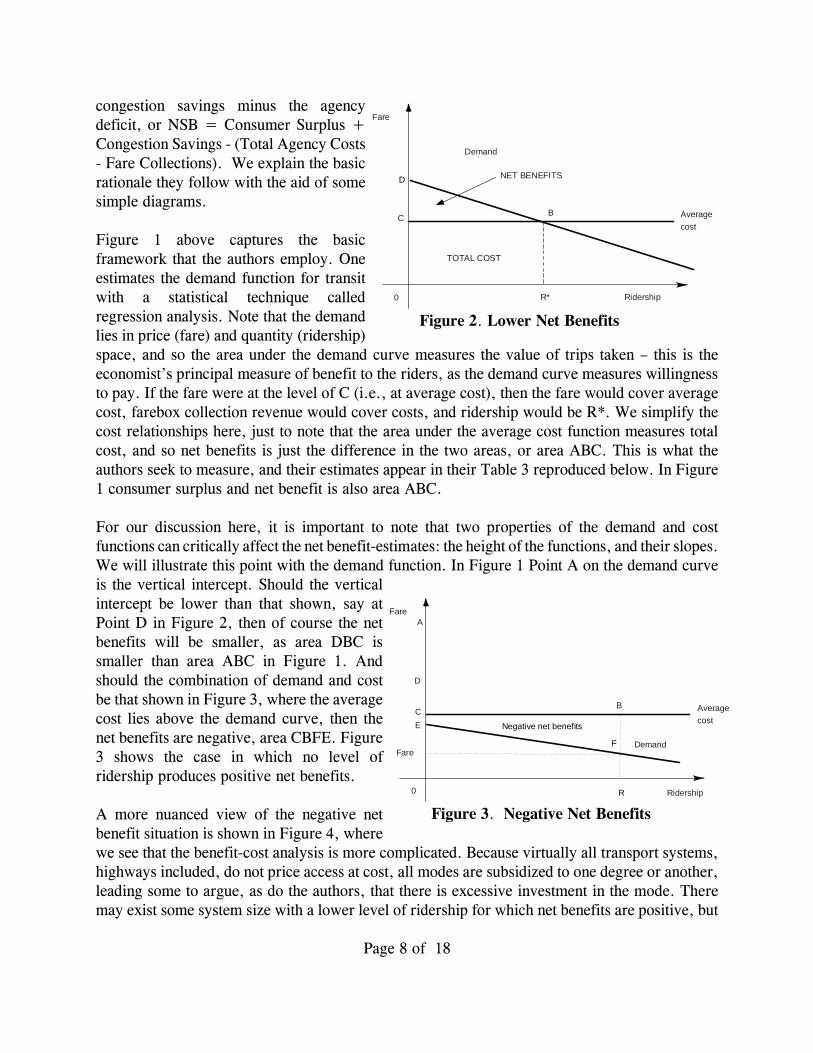
congestion savings minus the agencydeficit, or NSB = Consumer Surplus +Congestion Savings - (Total Agency Costs- Fare Collections). We explain the basicrationale they follow with the aid of somesimple diagrams.

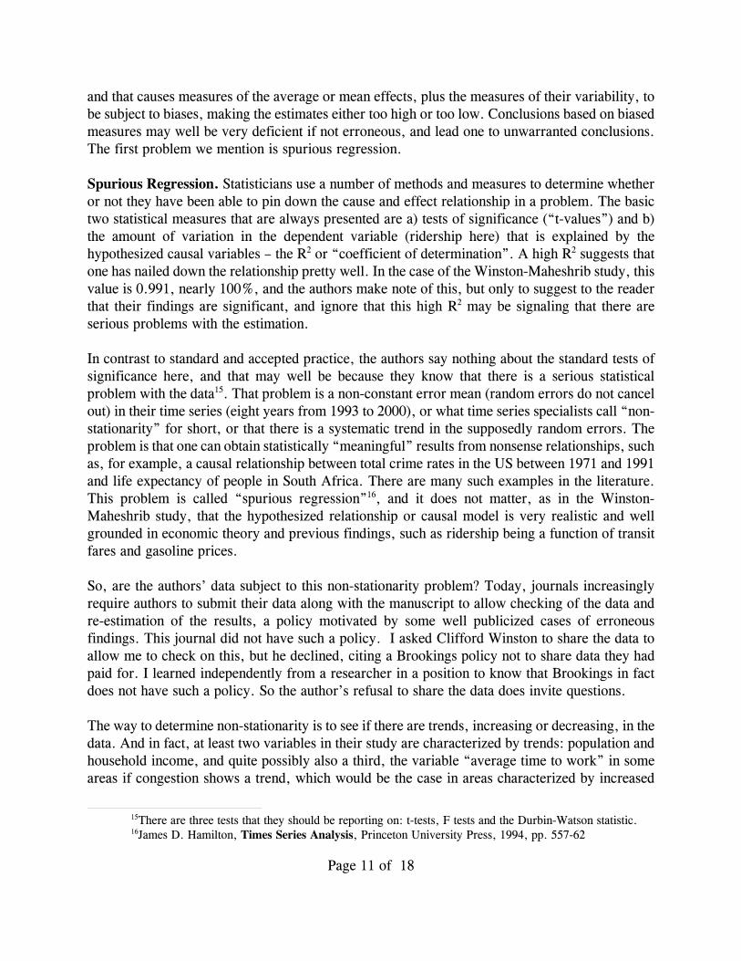
Figure 1 above captures the basicframework that the authors employ. Oneestimates the demand function for transitwith a statistical technique calledregression analysis. Note that the demandlies in price (fare) and quantity (ridership)space, and so the area under the demand curve measures the value of trips taken – this is theeconomist’s principal measure of benefit to the riders, as the demand curve measures willingnessto pay. If the fare were at the level of C (i.e., at average cost), then the fare would cover averagecost, farebox collection revenue would cover costs, and ridership would be R*. We simplify thecost relationships here, just to note that the area under the average cost function measures totalcost, and so net benefits is just the difference in the two areas, or area ABC. This is what theauthors seek to measure, and their estimates appear in their Table 3 reproduced below. In Figure1 consumer surplus and net benefit is also area ABC.

For our discussion here, it is important to note that two properties of the demand and costfunctions can critically affect the net benefit-estimates: the height of the functions, and their slopes.We will illustrate this point with the demand function. In Figure 1 Point A on the demand curveis the vertical intercept. Should the verticalintercept be lower than that shown, say atPoint D in Figure 2, then of course the netbenefits will be smaller, as area DBC issmaller than area ABC in Figure 1. Andshould the combination of demand and costbe that shown in Figure 3, where the averagecost lies above the demand curve, then thenet benefits are negative, area CBFE. Figure3 shows the case in which no level ofridership produces positive net benefits.

A more nuanced view of the negative netbenefit situation is shown in Figure 4, wherewe see that the benefit-cost analysis is more complicated. Because virtually all transport systems,highways included, do not price access at cost, all modes are subsidized to one degree or another,leading some to argue, as do the authors, that there is excessive investment in the mode. Theremay exist some system size with a lower level of ridership for which net benefits are positive, but

D

0

Fare

Ridership

Demand

Average

cost

BC

NET BENEFITS

R*

TOTAL COST

Figure 2. Lower Net Benefits

0

Fare

Ridership

Demand

Average

cost

A

BC

E

D

Fare

R

F

Negative net benefits

Figure 3. Negative Net Benefits

14 It is important not to confuse revenue with benefits. Revenue is about finance, and may or may notreflect the benefits accurately. In this case, it does not, and for that reason it is important to find the demand curveand measure the area under it. One can see that fare revenue in the general case underestimates the benefitsbecause it does not include the benefit triangle above the cost curve.

Page 9 of 18

because of the subsidy, the higherridership leads to excessive investment,running up the costs more than thebenefits. Net benefit in Figure 4 then isarea DBC minus area BGH. BGH is theexcess of cost over benefit (notrevenue) for the ridership between R*and R.14 In that figure, net benefit isshown to be negative. So whateconomic analysis attempts to ascertainare the relative sizes of the two areas.The authors in effect argue that BGH islarger than DBC for all cities analyzedexcept Chicago and San Francisco, andso the net benefits are said to be negative. As we show below, they make several errors thatmislead them to conclude that the situation is as in Figures 3 or 4. The way one translates the statistical findings to this net benefits framework is fairly simple. Theauthors estimate a linear relationship between ridership and its causal variables. That is, theyestimate an equation of the following form:

( ) ( ) ( ) ( ) .Ridership a b fare c gas price c population d income etc

The statistical analysis determines the values of the coefficients a, b, c, d, and also the signs ofthe estimated coefficients or parameters, positive or negative. Since the net benefits analysis isexpressed in fare and ridership space (price and quantity), this equation is solved (inverted) to findfare as a function of ridership, or

( )Fare ridership

This is a straight line shown as the demand curve in the previous figures. The value of " is foundby taking the average or mean values of the variables such as gas price, income, population, etc.,and multiplying them by the coefficients found for the ridership equation above and then addingthem together to generate ", which corresponds to the letters A, D or E in the above diagrams.

It is very important and central to these comments that if either the signs or the numerical valuesof the coefficients or both, are incorrect, then the net benefit calculation will be incorrect also.And the net benefit calculation may be very sensitive to alternative values of the estimatedcoefficients, especially if the data are very aggregated (one number per area per year) as they are

0

Fare

Ridership

Demand

A

BC

R*

Fare

R

G

H

AverageCost

D

Figure 4. Negative Nets Benefits

Page 10 of 18

in the Winston and Maheshrib paper. So one has to be very sure about the quality of the data,i.e., that they are proper measures of the influence of interest, and resulting estimates. One alsoneeds to do some sensitivity testing or analysis to check on how sensitive the net benefit calculationmight be to a range of values. There are ways to do this, but it should be noted that the authorsmention none of these, and so we conclude that they do not perform them. This in itself raisesquestions about the carefulness of the study.

In sum, before one can accept the author’s findings, one needs to be assured that the estimates ofthe demand and cost functions are valid, and not biased in one direction or another. A carefuleconometric analysis always discusses these issues, and the normal peer review is certain todemand this of manuscripts submitted to journals for possible publication. But curiously in thisarticle there is none of this discussion. This raises serious questions, and in fact we argue, thereare reasons to think that the authors’ findings are not valid and that they have underestimated thenet benefits, invalidating their conclusions. This article does not show the carefulness of analysisthat one would expect to support such strong conclusions and one is left to wonder about thequality of the peer review in this case.

Statistical Problems The statistical technique employed in the study is the standard approach to econometric estimation,that of regression analysis. For those not trained in statistics, we note that in all spheres of sciencethe way we pin down causality, that is, how the world works, is to observe a change in someindependent influence or variable, and measure the change in the response variable. In controlledexperiments, these changes are induced by the researcher. In natural experiments or observationalsituations, such as most of econometric analysis, one has to assemble the data on cause and effectvariables that theorizing tells us matter and are causal, and then analyze them statistically. Multipleregression is just a formal way of doing that when there are multiple influences that affect theresponse variable. That variable in this study is just ridership on the demand side, and cost on thesupply side.

Recalling that the authors did not have millions of dollars to conduct their study, they usedpublished data from various governmental sources. This is standard practice and all non-experimental measurements rely on historical observations. Critical to the ability to deducewarranted implications from the statistical analysis that can be used for policy recommendationsis that the data have to be, as statisticians say, “well behaved”, meaning that a number of statisticalproperties need to be satisfied. If they are not, then the findings may be meaningless. There is astrong possibility in the Winston-Maheshrib study that the findings are meaningless, since thereis one very important problem with their data that likely vitiates the conclusions they draw. Weexplain.

Without getting technical, since all real world variables and measurements are subject to randominfluences, statisticians have determined that the random errors in regression analysis on balancehave to cancel out in order for the estimations to satisfy several generally accepted properties.When they don’t, we say that there are systematic influences in the error term or error structure,

15There are three tests that they should be reporting on: t-tests, F tests and the Durbin-Watson statistic. 16James D. Hamilton, Times Series Analysis, Princeton University Press, 1994, pp. 557-62

Page 11 of 18

and that causes measures of the average or mean effects, plus the measures of their variability, tobe subject to biases, making the estimates either too high or too low. Conclusions based on biasedmeasures may well be very deficient if not erroneous, and lead one to unwarranted conclusions.The first problem we mention is spurious regression.

Spurious Regression. Statisticians use a number of methods and measures to determine whetheror not they have been able to pin down the cause and effect relationship in a problem. The basictwo statistical measures that are always presented are a) tests of significance (“t-values”) and b)the amount of variation in the dependent variable (ridership here) that is explained by thehypothesized causal variables – the R2 or “coefficient of determination”. A high R2 suggests thatone has nailed down the relationship pretty well. In the case of the Winston-Maheshrib study, thisvalue is 0.991, nearly 100%, and the authors make note of this, but only to suggest to the readerthat their findings are significant, and ignore that this high R2 may be signaling that there areserious problems with the estimation.

In contrast to standard and accepted practice, the authors say nothing about the standard tests ofsignificance here, and that may well be because they know that there is a serious statisticalproblem with the data15. That problem is a non-constant error mean (random errors do not cancelout) in their time series (eight years from 1993 to 2000), or what time series specialists call “non-stationarity” for short, or that there is a systematic trend in the supposedly random errors. Theproblem is that one can obtain statistically “meaningful” results from nonsense relationships, suchas, for example, a causal relationship between total crime rates in the US between 1971 and 1991and life expectancy of people in South Africa. There are many such examples in the literature.This problem is called “spurious regression”16, and it does not matter, as in the Winston-Maheshrib study, that the hypothesized relationship or causal model is very realistic and wellgrounded in economic theory and previous findings, such as ridership being a function of transitfares and gasoline prices.

So, are the authors’ data subject to this non-stationarity problem? Today, journals increasinglyrequire authors to submit their data along with the manuscript to allow checking of the data andre-estimation of the results, a policy motivated by some well publicized cases of erroneousfindings. This journal did not have such a policy. I asked Clifford Winston to share the data toallow me to check on this, but he declined, citing a Brookings policy not to share data they hadpaid for. I learned independently from a researcher in a position to know that Brookings in factdoes not have such a policy. So the author’s refusal to share the data does invite questions.

The way to determine non-stationarity is to see if there are trends, increasing or decreasing, in thedata. And in fact, at least two variables in their study are characterized by trends: population andhousehold income, and quite possibly also a third, the variable “average time to work” in someareas if congestion shows a trend, which would be the case in areas characterized by increased

Page 12 of 18

sprawl, and increased population.

Now this problem of non-stationarity is well known, as is the remedy: simply difference the series,that is, subtract adjacent values from one another and use the resulting differences to estimate theregression. The authors did not do this, nor do they indicate why not, and this then is another issuethat raises concerns about the validity of the findings. The authors’ main findings on ridershipappear in the following table taken from the published article. Even before we get to discussingthe implications for the estimated benefits, we note the high R2 is inflated for two reasons: the non-stationarity problem, and the fact that the data are very highly aggregated (one observation permetro area per year). The test of the statistical significance of the entire relationship as a whole,that, all the variables in the regression equation taken together, is the F test. It is closely relatedto the R2 and had they presented it, it too would be quite high, but also quite meaningless, as thenon-constant error mean results in artificially inflated F tests. Again, presentation of this test valueis standard operating procedure, and the fact that it is not reported has to raise concerns about thefindings.

Hypothesized Effects:Measurement and DataProblems The standard way theseanalyses are conducted, byeconomists at least, is to useeconomic theory to specify therelationship (what causeswhat), and also to indicate inadvance what the expecteddirection of the causalinfluence is, that is, whetherthe effect is expected to bepositive or negative. Themagnitude of the effect isfound from the statisticalanalysis. Often the underlyingtheory is fairly clear about thedirection of the effect, suchas, prices are always inverselyrelated to quantity demanded,or in this case ridership andfares are negatively related.

But frequently the a priorieffect direction is not clear,and so the author will indicate

17http://www.eia.doe.gov/emeu/aer/txt/ptb0524.html

Page 13 of 18

that it can go either way, and offer some reasons why it might go in either direction. The problemhere is that indicating no clear a priori direction can just be a cover hiding problems with themodel or the data or both. Often if not usually, the researcher (especially economists) will havea theoretical reason to expect a positive or a negative influence, but once he or she sees that theresults of the analysis do not support that, then one says that the result is “unexpected” or“surprising”, language that appears frequently in empirical papers. Or, the author may go backto the section on expected a priori effects and revise it with some language indicating why it mightgo each way.

This kind of back and forth between theorizing and findings is common in all sciences, but it isimportant to think through the reasons for the direction of the causality. In this case, it is clear thatthe authors have not spent much time on this and calls into question their findings. We explain thisnext, focusing on two important causal influences: gas prices and average commute time, andindicate what the implications are.

Regional gasoline prices. Generally speaking, as a microeconomic analysis (individual decisionmaking), road trips and transit trips are substitute commuting modes, as we saw everywhererecently as gasoline prices rose. Of course, park and ride facilities combine road and transit trips,but the focus is on the main commuting mode. As substitutes, we would expect to see transitdemand rise when gasoline prices rise, so the sign of the gasoline price coefficient in theregression should be positive: higher gas prices cause increased transit demand. Winston andMaheshrib do not report their data, but an examination of a gasoline price series from theDepartment of Energy shows that from 1993 to 2000, gasoline prices were essentially flat, fallinga bit at the beginning of the period. The then current dollar prices (unadjusted for inflation) duringthe period lay between $1.09 and $1.47.17 Gasoline was cheap.

But, as one of those statistical “surprises”, they find the coefficient to be negative, giving an cross-price elasticity of demand for the sample period of - 0.703 (my calculation from their reporteddata). This is inelastic, meaning that a 10% increase in gas prices will lead to a less thanproportionate 7% decrease in transit ridership. While the magnitude of the effect seemsreasonable, the sign really is unexpected, and so this qualifies as a “puzzling” and “surprising”result, although the authors do not say that.

In these circumstances, the careful researcher goes back and asks what factor or factors mightexplain this result, as well as scrutinizing the data to see if there is something peculiar about thedata and how they are measured that might lead to the result . Often one can make a plausibleconjecture. In this case, the authors conjecture that high gas prices can depress regional economicactivity, and that could account for the negative coefficient, when a positive one would normallybe expected. And it is true that high energy prices can have major macroeconomic effects, as wesaw in the mid 1970's and early 1980's, and as we see now.

18http://www.gpoaccess.gov/eop/tables08.html

Page 14 of 18

The only problem with their alternative hypothesis is that their period of 1993 to 2000 starts afterthe recession in 1991, and the Economic Report of the President18 shows a prolonged economicexpansion and rising employment, which the readers will recall was the period of stock marketexuberance driven by the technology sector. So that explanation would not seem to work, but theauthors evidently and surprisingly did not examine it further. So one is left with an unexplainedfinding. This well could be a result of the non-stationarity of the random errors, as discussedabove, or a problem with the data. Their surmise could have easily been tested by including ameasure of labor market conditions in the regressions, but they do not do this.

Now, as we discussed above, this issue is very important to the basic thrust of the paper, becausein their calculation of the benefits a negative coefficient on this variable means that the estimateddemand curve is shifted down (the cases illustrated in Figures 2, 3 and 4), incorrectly we arguehere. That leads to a lower computed (and underestimated) value of the benefits of the transit, andcertainly has to be a contributing factor to the authors’ generally negative findings concerning thebenefits of transit.

The data set is a panel, which means that it contains both longitudinal values (over time), andcross-sectional values (across space). There is significant variation in gasoline prices across thenation, mostly due to differences in state excise taxes on gasoline, and in the cost of fuel transportif the region does not have nearby refineries. Could this variation cause the negative relationshipbetween transit ridership and gas prices? We do not know, as the authors neither mention norexamine it. I am unaware of any study that connects state gasoline taxes and transit ridership, butthe problem with even this argument is that the generalized anti-tax political climate of the last fewdecades has led most states to freeze their gasoline taxes, and so the real (inflation adjusted)gasoline tax has been falling relative to the growth in income. If it were true that the states withhigher gasoline taxes were also the ones with lower transit demand, that could conceivably providethe cross-sectional variation to produce the negative coefficient. That was not examined, and onecould argue the converse, that those states with high taxes are the ones with large highwayconstruction budgets, and those investments would be concentrated in congested cities, but this isjust speculation. The authors could and should have examined this issue, but did not. So we areleft with an implausible result, and no good explanation. One suspects a faulty model and data.

Commute time. That leads us to another important variable in the paper, average commute time.High commute times in metropolitan areas are associated with congestion. All else equal, giventhat road and transit trips are substitute modes for those living in the transit corridors, thepredicted commuter behavioral response in the presence of frequent and expected highwaycongestion would be increased demand for transit, as transit lines never get congested because theheadways are controlled (although the transit cars can be crowded) – thus the run times are fairlyconstant and quite predictable. As a result, the predicted effect of road congestion on transitdemand should be positive. But again, as with gas prices, the authors instead suggest that the effectcould go either way: positive or negative. They speculate that high road congestion can reduce

19“The demand for rail has continued to shrink because transit networks are unable to keep upwith changing land use and travel patterns that have decentralized residences and employment”. Page 379. They donot mention that it is highway investments that are major drivers of this decentralization.

Page 15 of 18

accessibility to transit stations, but offer no evidence for this hypothesis. But even if highwaycongestion did reduce access to park and ride facilities, it does not follow that remaining on thecongested highway is a time saving strategy for journeys to work.

The authors in fact find the opposite, that increased congestion leads to lower, not higher, transitridership. To illustrate the finding, we compute the implied cross elasticity of transit demand withrespect to average commute time using their reported mean values. Using both the linear andsquared terms, this elasticity is - 0.09. That is, their results indicate that a 10% increase in meancommute time or congestion leads to a about a 1% decrease in transit demand. To say the least,this is counterintuitive, and most likely is evidence of either serious data problems or faulty modelspecification, or both. Their explanation does appear to be an after-the-fact explanation foranother “puzzling” result. And since the widely used transit demand planning models, which arebased on detailed mode choice behavior, generate the benefits of transit based precisely due toreduced travel time on rail, this finding flies in the face of the established and widely used tripgeneration models.

A proper test of the relationship between road congestion and transit demand would require dataon commuter travel in the corridors that contain both highways and transit lines. Congestion onroads in other corridors would not be relevant. But the data the authors employ measure theaverage commute time for the entire metropolitan area (one observation per metropolitan area peryear), which also includes highway corridors without competing transit lines. So if congestion issevere and growing in those corridors without rail transit alternatives, as it has been, andpopulation is decentralizing to areas without rail transit alternatives because of suburban highwayinvestment, which it has as the authors point out 19, with the measure the authors employ, it isindeed possible to find a negative relationship between transit ridership and average commute time,that is, a correlation, but without any reason to suggest causality. This is because much or mostof the congestion will be measured in non-rail transit corridors, and with the decentralization ofpopulation over time in the older transit systems to areas not served by rail, ridership will belower. The problem here is that the commute time variable they employ is inappropriate for theanalysis and leads to incorrect findings.

This has the same serious implication for the benefits calculation as the gasoline price case. Anegative net sign on this pair of coefficients (for the linear and squared values) means that thedemand function for transit is shifted down, and the estimated benefits reduced. But if the sign isnot plausible, as we argue here, then the authors’ benefit estimates are biased downward, leadingto incorrect conclusions.

Mode Reliability. Related to commute time variable is the issue of the reliability of commutingvia highway or transit. Commuters value not only short commutes, but reliable commutes.

Page 16 of 18

Reliability or risk is typically measured by the variability of the commute times, or whatstatisticians call the variance, yet the authors include no measure of variability of commute times,except across regions and over time. But their measure does not capture the correct dimension.We would expect that greater variability in trip times or lower reliability of highway commutingwould lead to greater transit demand, and the failure to include this variable leads to the ratherserious problem of “omitted variable bias”. This is a major omission. Since a variable measuringrelative mode reliability of transit would by hypothesized to have a positive coefficient, excludingit means that this represents a possible third reason why their demand and benefit measures wouldbe biased downward.

Nonetheless, at this point, it is a relatively safe argument that the authors’ benefit estimates areseverely biased downward, and that would be one reason why they find negative net benefits formost systems. Their conclusions are erroneous as a result. The authors paid far too little attentionto the quality of their data, and to whether the chosen variables or data measures were in fact wellmatched to the problem they sought to investigate. It is a puzzle how this got through the peerreview process, on which we comment at the end.

Authors’ Conclusions on the net benefits of rail systemsThe measured net benefits of the systems the authors examine depend crucially on the statisticalresults, that is, the numerical values and signs for the parameters of the demand functions, whichwe noted above may well be totally meaningless in their study. If that were not enough, theauthors’ less than careful discussion of the net benefits of the systems adds to the doubts about thevalidity of the findings. We explain briefly.

Sensitivity Analysis. First, all measurements and estimates of real world relationships are subjectto error. There are many types of measurement and estimation errors statisticians have identified,and so if one is to use statistical estimates to inform any decision, such as a public policy decisionconcerning transport investments, it is always appropriate to estimate the risks, and theconsequences, of a wrong decision. “Risk” just means variable outcomes. The standard approachto this problem is to conduct a random scenario analysis, called Monte Carlo analysis, that showsthe variability and the impacts on the benefit estimates. The authors do not do this.

Additionally, a careful benefit-cost analysis always presents a discussion of those variables thatthe authors have not been able to include, usually for lack of data availability. Such a discussionincludes a listing of these excluded variables and the likely impacts or implications of theexclusion. This is critical, because of the omitted variable bias mentioned above, and we illustratewith the variable of highway lane miles.

This “omitted variable” problem seems to be present in this study. This potentially seriousomission is that they do not include highway expansions (lane miles) in the variable set. Roadtraffic and transit ridership are jointly determined, in which the time and money cost of one modeaffects the demand for the substitute mode. In the period they study, 1993 to 2000, there wasimportant economic growth throughout the country, populations continued suburbanizing, and

20See the Transit Cooperative Research Program report 78, “Estimating the Benefits andCosts of Public Transit Projects: A Guidebook for Practitioners” Transportation Research Board, NationalAcademy of Sciences, 2002.

Page 17 of 18

urban highway capacity was added, but only in a few new systems has track capacity beenexpanded. More highway lane miles leads to lower transit ridership as it can reduce roadcongestion in the short run (a period of several years), thus reducing the time and money costs ofhighway commutes. So there is a negative influence that appears in the ridership numbers, but noindependent causal variable designed to capture and measure it. This means that one or more ofthe estimated parameters are in error, either the sign, or the magnitude, or both. In this case, theinfluence of this omitted variable may be weakly captured in the variable “average time to work”,but we cannot know without a complete analysis of the relationships without the variable. In amultiple regression it is a very tedious exercise to work out the effect of this bias analytically, thatis, by hand.

Further, as noted, road traffic and transit ridership are jointly determined. That raises still anotherproblem, called simultaneous equation bias, which also has the effect of generating biased valuesfor the responsiveness of ridership to variation in fares and other influences such as gasoline pricesand congestion.

This matters to the benefit-cost analysis in this way: a relevant question for transport investmentsis what would have happened to transit ridership had the additional investments in highwayexpansions not taken place. Multiple regression always allows one to provide some answers to thatquestion, which would be critical to the conclusions that the authors draw.

Option Value. Another dimension of careful benefit-cost analysis is attention to those benefit andcost dimensions that are not captured with the techniques they employ. For example, peoplegenerally like to have options when making choices, both now and in the future. So in generaleven those who currently choose to commute by auto would be generally willing to pay somepositive amount to ensure that other transit options remain open to them should they be unable orunwilling to drive at some future time, due to such factors as car repairs, highway construction,incapacitating health conditions, etc.

Logically then economists call this “option value”, and this value is not picked up in the demandfunction that the authors estimate. There are many options markets and have been the object ofmuch study. There are suggested techniques for the transit case20, which would not have requiredmuch additional work to apply in this study. But at a minimum the issue should have beendiscussed, with the observation that those benefits that they did estimate are too low because ofthe exclusion of option value.

Further, they could have asked the question about how large option value would have to be inorder for the net benefits in their study to be positive. In this case, the estimate would be too largebecause, as we have argued above, their net benefit estimates are biased downward, and are toolow.

Page 18 of 18

Conclusions

In summary, while at first blush Winston and Maheshri’s study seems carefully done, in fact itcontains significant biases and omissions. It only considers a minor portion of rail transit benefitsand ignores the indirect social benefits that result when rail transit provides a catalyst for morecompact development. It overlooks trends that are increasing demand for high quality public transitservice and transit oriented development. As a result, rail transit investments tend to provide fargreater total benefits than the study assumes.

There are some relatively elementary statistical issues that were not explored, or at least, noreasons were presented indicating why they were not, and so on this basis alone it isinappropriate and unwarranted for the authors to reach the conclusions they do: that virtuallyall of the rail systems are net losers.

In fact, this seems less than a carefully done analysis. When asked why he did not present thestatistical tests mentioned above, Winston’s reply was that the data series is too short to presentthese problems. That is possible, but not one that the profession would take on faith, and soevidence should be provided. The tests should have been done and the fact that they were notproperly and normally raises questions about the validity of the findings as well as aboutpotential biases.

Finally, how did this get through the review process? That is for the journal editor to answer,but having participated in conference volumes before, the answer quite likely is that the normalreview process was not applied here, but something less exacting. At least this manuscriptwould not have made it by this reviewer without a very substantial “revise and resubmit”recommendation to the editor. We have to conclude that this study has multiple seriousshortcomings and should not be used to draw conclusions about the direction of investments inthe nation’s transport system, especially not in this time of rising energy prices.