A Revisit to the Markup Practice of Dynamic Pricing

Yifeng Liu∗ and Jian Yang†

Department of Management Science and Information Systems

Business School, Rutgers University

Newark, NJ 07102

Emails: ∗yifeng@pegasus.rutgers.edu and †jyang@business.rutgers.edu

March 2012; revised, December 2012, July 2013, March 2014

Abstract

In this article, we focus on the markup practice of dynamic pricing in which a firm uses

real-time inventory information to decide the most opportune time to raise its sales prices. In

our model, demand arrives as a Poisson process in which the instantaneous rate is a product of

two terms, one dependent on current price and the other on present time. Through a mixed use

of mathematical induction and sample-path arguments, we establish the optimality of threshold

policies. Under such policies, the firm would base its price-switching decision on a comparison

made between the present time and the threshold level corresponding to the present price and

inventory level.

Feng and Xiao [5] have studied a stationary version of this problem along with the opposite

markdown case. Though the earlier work has made dramatic advances in dynamic pricing and

has pioneered many relevant techniques, we believe its treatment of the markup case warrants

some revision. In particular, we find that the markup case is in possession of the erstwhile-

unknown complementarity between price flexibility and inventory, a property whose counterpart

is not true for the markdown case. Our development also leads to an efficient policy-computing

algorithm.

Key words: Dynamic Pricing; Markup Practice; Threshold Policy

1

1 Introduction

Dynamic pricing is mainly concerned with how a firm can maximize its revenue by charging the

right prices over a fixed time horizon, given that demand arrives in a random and yet price-sensitive

fashion. This paper focuses on the case where the concerned firm is in the markup mode, so that

it continuously charges a sequence of progressively raised prices. Airlines and hotels often practice

markup to sell tickets to exploit the difference in cost sensitivity between leisure and business

travelers. Obviously, a firm may also exercise markdown, or, when there is no predetermined

direction in which prices can go, reversible pricing.

In this study, we analyze a firm that faces Poisson demand and sell a finite initial inventory

over a fixed time horizon. It is allowed to charge prices from a given set pk|k = 0, 1, ....,K in the

increasing order p0, p1, ..., pK over time. The Poisson arrival rate of demand follows the product

form λk(t) = αk · β(t): the overarching time-dependent term β(t) spells out demand’s oscillation

over time, and the actual arrival rate is proportional to both this term and the price-dependent

factor αk. We establish the optimality of a threshold policy, with the latter representable by time

points τkn that depend on both prices k and inventory levels n and satisfy τkm ≤ τkn for m ≥ n. The

firm should start to charge the next higher price when the decline of its inventory level has pushed

the threshold point associated with the current price and inventory level behind the current time.

The above can be viewed as a generalization of the markup portion of Feng and Xiao’s [5] result

concerning the price-sensitive but time-independent demand pattern. Using almost symmetric

arguments, these authors also established the optimality of threshold policies for the opposite

markdown practice, in which a firm charges prices in decreasing order over time. As an equally

important contribution of ours, we point out that the symmetric treatment is problematic. For the

markup case, we note the following two main points based on our own derivation:

(i) The value function vkn(t) has decreasing differences between k and n (Proposition 3).

(ii) The above point is crucial for the proof of the optimal policy, which was previously ignored

in Feng and Xiao [5].

A counter example of a technical result in Feng and Xiao [5] is given in Appendix D. For the

seemingly symmetric markdown case, the counterpart to (i), that vkn(t) has increasing differences

between k and n, is neither true nor needed in the derivation involving its threshold policies.

We also show that the threshold policy is not necessarily monotone in k; that is, the seller may

prefer to skip certain price levels. In an online supplement, we work out details for the markdown

case. There, efficient algorithms for computing threshold levels are developed as well.

Now let us briefly recount earlier research on dynamic pricing. Gallego and van Ryzin [6] started

treating dynamic pricing from the optimal control perspective. They examined the problem of

dynamically pricing inventories with stationary, stochastic demands, and showed the optimality of

a monotone pricing policy as well as the asymptotic optimality of fixed-price heuristics. Dealing

2

with a similar model with a finite number of price choices, Feng and Xiao [4] justified the earlier

assumption that the revenue-generation rate increase and be concave in the demand arrival rate.

They derived the optimality of a comparable monotone pricing policy and offered a procedure for

computing this policy.

When demand is time-varying, Zhao and Zheng [8] identified the decline over time of customers’

willingness to pay premiums as a sufficient condition for the monotonicity of the optimal pricing

policy. This result generalizes the claim made by Bitran and Mondschein [1] that a monotone

policy would be optimal when the ratio of arrival rates at any two given prices remains the same

over time. For a multi-product/resource version of the problem, Gallego and van Ryzin [7] gave

asymptotically optimal heuristics that are based on the solution to the problem’s deterministic

control counterpart.

Feng and Gallego [2] initiated irreversible pricing control with their study of a problem involving

two price choices and an arrival pattern that is dependent on price only. For this problem, they

showed the optimality of a threshold-like policy. Feng and Xiao [5] generalized the above result to a

case with multiple price switches in the same direction. Feng and Gallego [3] moved on to the more

general problem where both paths of prices and arrival rates can be time-varying, and demand

may be dependent on sales-to-date. For this case, however, optimal policies were not shown to

necessarily come from the threshold-like family.

The current paper can be considered as both a generalization to the product-demand form

and a correction to the markup portion of Feng and Xiao [5], which in both irreversible pricing

cases arrived at the same conclusion on the threshold-like policy shape. Our derivation, however,

sheds more light on the distinction between the markup and markdown cases. As a property,

complementarity between price flexibility and inventory is not possessed by the markdown case;

yet, it is essential to the derivation for the markup case. Feng and Xiao’s [5] treatment of the

markup case seems to have missed this point.

Methodologically, we introduce a mixed use of mathematical induction and sample-path ar-

guments to facilitate the derivation of the complementarity property. Additionally, we show that

overall τkn is not decreasing in k for the two irreversible pricing cases, though for the reversible

pricing case this trend, known as time monotonicity, exists (Zhao and Zheng [8]).

The rest of the note is organized as follows. In Section 2, we provide the problem’s formulation.

We propose a procedure for constructing value functions and threshold levels in Section 3, and prove

the optimality of the thus constructed threshold policy in Section 4. We then discuss merits of our

current approach in Section 5. The note is concluded in Section 6. We have relegated technical

details to appendices in the end. More developments regarding the markdown case and algorithms,

as well as numerical results are contained in the online supplement.

3

2 Formulation

Over some time interval [0, T ], we suppose that the concerned firm is to sell N items of a product

and that it is allowed to consecutively charge a sequence of K + 1 prices p0, p1, ..., pK , where

0 < p0 < p1 < · · · < pK . Demand comes to the firm as a time-varying Poisson process whose

instantaneous rate λk(t) depends on both the current price pk charged by the firm and the overall

market condition at time t. We also suppose that the demand rate function is of the product form.

We place strictly positive constants α0, α1, ..., αK and strictly positive and continuous function β(·)on [0, T ], so that

λk(t) = αk · β(t), ∀k = 0, 1, ...,K, t ∈ [0, T ].

The time multiplier β(·) may be a consequence of seasonality of the product being sold, the fact

that the concerned product is newly introduced or is gradually phasing out of the market, or other

factors such as predictable changes over time of the competitive firms’ aggregate behavior. The

price multiplier αk indicates the relative attractiveness of the product under price pk.

We assume that:

(S1) for the revenue generation rates,

p0α0 > p1α1 > · · · > pK αK .

(S1) lets lower prices be associated with higher revenue generation rates, since there would be no

need to consider a lower price if it did not generate revenue faster than a higher price. In case

prices p form a continuum and the arrival rate function is λ(·), the counterpart to (S1) would be

(pλ(p))′ < 0, which could be rewritten as

−λ′(p)λ(p)/p

> 1. (1)

In economics terms, the assumption states that demand for the concerned product is elastic. Clearly,

(S1) would lead to the weaker

(S1’) for the demand arrival rates,

α0 > α1 > · · · > αK .

We take the view that potential buyers arrive at the rate of α0 ·β(t) at time t, and among all those

that arrive, only a αk/α0 portion will purchase the product when the price being charged is pk. We

now define λ, so that

λ = α0 · supt∈[0,T ]

β(t). (2)

By the continuity of β(·) and the compactness of [0, T ], we know that λ is a strictly positive and

finite constant. By (S1’), we know that λ is the highest instantaneous arrival rate that can ever be

achieved.

4

We denote a threshold policy by τ = (τkn | k = 1, 2, ...,K, n = 1, 2, ..., N) ∈ (∆N )K , where

∆N ⊂ [0, T ]N is defined through

∆N = (τ1, τ2, ..., τN ) | 0 ≤ τN ≤ τN−1 ≤ · · · τ1 ≤ T. (3)

For the current markup case, adopting such a policy entails that the firm should raise its price from

pk−1 to pk when its inventory level drops to n ahead of the threshold level τkn .

Throughout, we define all random elements on a probability space (Ω, P,F) that is equipped

with a filtration (Ft | t ∈ [0, T ]). Each price choice k is associated with a point process (Nk(t) |t ≥ 0) that has intensity process (αk · β(t) | t ∈ [0, T ]) and is adapted to the given filtration. For

any s < t, the increment Nk(t)−Nk(s) is independent of Fs while for n = 0, 1, 2, ...,

P [Nk(t)−Nk(s) = n] = exp(−αk · β(s, t)) · (αk · β(s, t))n

n!. (4)

In (4), we have taken the conventions 00 = 1 and β(s, t) =∫ ts β(u) · du.

Let vkn(t) be the maximum revenue the firm can make in time interval [t, T ] when it starts the

interval with price pk and inventory level n. As the highest price pK is the last price for the firm

to charge, we have

vKn (t) = pK · E[(NK(T )−NK(t)) ∧ n]. (5)

For k = K − 1,K − 2, ..., 0, the firm still has the chance to increase its price to pk+1 when it is

currently charging pk. Hence,

vkn(t) = supτ∈T (t)

E[pk · (Nk(τ)−Nk(t)) ∧ n+ vk+1(n−Nk(τ)+Nk(t))+(τ)], (6)

where T (t) is the set of stopping times later than t.

3 A Constructive Procedure

We define the infinitesimal generator Gkn(t) corresponding to price pk, inventory level n, and time t,

so that when it is applied to a well-defined function vector u = (un(t) | n = 0, 1, ..., N, t ∈ [0, T ]),

Gkn(t) u = dtun(t) + αk · β(t) · (un−1(t)− un(t)). (7)

We think it is an abuse of notation to call the left-hand side Gkun(t), because knowing un(t) at the

particular n and t alone would not help one get to the right-hand side.

For the case where the time multiplier β(·) is stationary, Theorem 1 of Feng and Xiao [5] offers

sufficient conditions for a vector of functions to be the value functions vkn(t). But this result can

be easily generalized for the case where β(·) is time-variant. In the same spirit of this theorem, we

find the following.

5

Proposition 1 For any k = K − 1,K − 2, ..., 0, a function vector u ≡ (un(t) | n = 0, 1, ..., N, t ∈[0, T ]) that is uniformly bounded and absolutely continuous in t for every n will be vk ≡ (vkn(t) |n = 0, 1, ..., N, t ∈ [0, T ]), if it satisfies the following:

(i) un(t) ≥ vk+1n (t) for every n = 0, 1..., N and t ∈ [0, T ],

(ii) un(T ) = 0 for every n = 0, 1, ..., N and u0(t) = 0 for every t ∈ [0, T ],

(iii) for n = 1, 2, ..., N and t ∈ [0, T ], un(t) = vk+1n (t) implies Gkn(t) u+ pkαk · β(t) ≤ 0,

(iv) for n = 1, 2, ..., N and t ∈ [0, T ], un(t) > vk+1n (t) implies Gkn(t) u+ pkαk · β(t) = 0.

Proposition 1 offers a hint as to how the value functions vkn(t) and threshold levels τkn can be

constructed. First, due to (5) and the fact that vK0 (t) = 0, we can establish all the vKn (t) values in

an n-loop. Then, for any k = K − 1,K − 2, ..., 0, suppose vk+1n (t) is known for all n and t. We can

now go through an n-loop to find all the vkn(t)’s. First, we can let vk0 (t) = 0 as suggested by (ii)

of the proposition. Second, suppose vkn−1(t) is known for all t and some n = 1, 2, ..., N . Then, we

have vkn(T ) = 0 by (ii) of the proposition. Next, we may “weave” vkn(t) for ever smaller t values by

solving the differential equation Gkn(t) vk + pkαk · β(t) = 0 as indicated by (iv) of the proposition.

We stop at the t when vkn(t) is to sink below vk+1n (t), which is not allowed by (i) of the proposition.

For time t′ earlier than this t, which we mark as τk+1n , we let vkn(t′) be vk+1(t′).

According to (iii) of the proposition, we still need Gkn(t′) vk + pkαk · β(t′) ≤ 0 for t′ < τk+1n

for the thus constructed vkn(·) to be the true value function. Nevertheless, let us proceed with

the construction procedure thus outlined. Not knowing whether what shall be constructed are the

true value functions, we call them u’s instead of v’s. Formally, here is the iterative procedure for

constructing function vector u = (ukn(t) | k = 0, 1, ...,K, n = 0, 1, ..., N, t ∈ [0, T ]) and point vector

τ = (τkn | k = 1, 2, ...,K, n = 1, 2, ..., N).

First, let

uk0(t) = 0, ∀k = K,K − 1, ..., 0, t ∈ [0, T ]. (8)

Then, for n = 1, 2, ..., N and t ∈ [0, T ], let

uKn (t) = αK ·∫ T

tβ(s) · (pK + uKn−1(s)) · exp(−αK · β(t, s)) · ds. (9)

Next, we go over an outer loop on k = K − 1,K − 2, ..., 0 and an inner loop on n = 1, 2, ..., N . At

each k and n, first let

ukn(t) = αk ·∫ T

tβ(s) · (pk + ukn−1(s)) · exp(−αk · β(t, s)) · ds, ∀t ∈ [0, T ]. (10)

Then, let

τk+1n = inft ∈ [0, T ] | ukn(t) > uk+1

n (t), (11)

with the understanding that τkn = 0 when the concerned inequality is always true and τkn = T when

it is never true. Finally, let

ukn(t) = uk+1n (t), ∀t ∈ [0, τk+1

n ]. (12)

6

The procedure we have outlined mainly goes through a k-loop to “weave out” the value func-

tions. This is similar to what Feng and Xiao [5] have done. It is interesting to note that the

procedure has no use for the differentiation operator, as it might be bad for numerical imple-

mentation. This presents a contrast to Feng and Xiao’s procedure, which in step k involves the

differentiation of uk+1n (t); see their Theorem 2.

In obtaining the integral forms (9) and (10), we have relied on an ordinary differential equation

(ODE) and its known solution. Given continuous functions a(·) and b(·) defined on the interval

[0, t], consider the following differential equation:

dsf(s) = b(s)− a(s) · f(s), ∀s ∈ (0, t). (13)

This ODE has a unique solution f(·), so that for any s ∈ [0, t],

f(s) = f(0) · exp(−∫ s

0 a(u)du) +∫ s

0 b(u) · exp(−∫ su a(v)dv) · du

= f(t) · exp(∫ ts a(u)du)−

∫ ts b(u) · exp(

∫ us a(v)dv) · du.

(14)

4 Optimality and k-Monotonicity

We now move on to show that the above procedure indeed leads to the true value functions and

an optimal pricing policy. First, through a sample-path argument that is reminiscent of Zhao

and Zheng’s [8] treatment of the same property for reversible dynamic pricing, we show that the

marginal value of any additional item is diminished at a higher inventory level.

Proposition 2 For any fixed k = 0, 1, ...,K and t ∈ [0, T ], the value function vkn(t) is concave in

n.

We can use this result and more involved sample-path analysis combined with mathematical

induction to show the added benefit that more flexibility in pricing can bring to the firm when

there are more items in stock.

Proposition 3 For any fixed t ∈ [0, T ], the value function vkn(t) has decreasing differences between

k and n.

Proposition 3 would play a critical role in the proof of the next key result. Its proof boils down

to an induction process that for n = 0, 1, ..., N − 1, shows

vkn+1(t)− vkn(t) ≥ vk+1n+1(t)− vk+1

n (t), ∀k = 0, 1, ...,K − 1, t ∈ [0, T ]. (15)

When proving (15) for each individual n, we borrow the sample-path idea from Zhao and Zheng [8].

In addition, both Proposition 2 and the same induction hypothesis (15) at inventory levels strictly

below n would find their use in the proof. We believe the property presented in Proposition 3 is

7

previously unknown; for instance, it is never mentioned in Feng and Xiao [5]. Interestingly, the

seemingly symmetric markdown case does not include the counterpart to this property. Indeed, our

computational study has shown that the markdown case does not hold complementarity between

price flexibility and inventory.

We further demonstrate the optimality of a threshold policy for the markup case. For con-

venience, we have let the yet undefined τK+1n = 0 for n = 1, 2, ..., N and vK+1

n (t) = uKn (t) for

n = 0, 1, ..., N and t ∈ [0, T ].

Theorem 1 The u and τ as constructed from (8) to (12) satisfy the following for k = K,K−1, ..., 0:

(a[k]) for any n = 1, 2, ..., N , (Gkn)+(τk+1n ) vk+1 + pkαk · β(τk+1

n ) ≤ 0;

(b[k]) Gkn(t) vk+1/β(t) is increasing in t for n = 1, 2, ..., N and t ∈ (0, T );

(c[k]) ukn(t) = vkn(t) for any n = 0, 1, ..., N and t ∈ [0, T ];

(d[k]) for any n = 1, 2, ..., N , we have vkn(t) = vk+1n (t) and Gkn(t) vk + pkαk · β(t) ≤ 0 for

t ∈ (0, τk+1n ), and Gkn(t) vk + pkαk · β(t) = 0 for t ∈ (τk+1

n , T );

(e[k]) τk+1n is decreasing in n;

(f[k]) on top of vkn(t) having decreasing differences between n and t, it is further true that

dtvkn(t)/β(t) is decreasing in t for n = 1, 2, ..., N and t ∈ (0, T ).

As a consequence, τ provides an optimal policy for the firm; under this policy, the firm should

switch to price pk+1 when its inventory level drops to n before time τk+1n while its price level is pk.

In (a[k]) of Theorem 1, the operator (Gkn)+(t) is merely Gkn(t) defined in (7) with dt replaced

by the right derivative d+t . The proof of Theorem 1 depends very much on the complementarity

property provided by Proposition 3. As an induction process over k = K,K − 1, ..., 0, it uses the

validity of (a[k + 1]) to (f[k + 1]) to show the validity of (a[k]) to (f[k]) for each k. When proving

the essential property (e[k]), that τk+1n is decreasing in n, one logical step we take is from that

vkn(t)− vk+1n (t) > 0 to that vkn+1(t)− vk+1

n+1(t) > 0. What facilitates this step is Proposition 3, that

vkn(t) has decreasing differences between k and n.

Finally, regarding the k-monotonicity of the optimal policy, we gather the following result

directly from the definition (11) and Theorem 1.

Proposition 4 Suppose τkn < T for some k = 1, 2, ...,K − 1 and n = 1, 2, ..., N . Then, we have

τk+1n ≤ τkn if and only if vk−1

n (t)− vkn(t) > 0 would lead to vkn(t)− vk+1n (t) > 0.

The condition specified above is almost that of vkn(t) being quasi-concave in k. However, as

prices and rates are only regulated by assumption (S1), there is no reason to believe this would be

the general case. Looking at it from another angle, we see that the triggering event for any price

switch is quantum in nature, as it involves the departure of an entire item of which the firm has

only a finite stock. Meanwhile, pk+1 might be only a tiny bit above pk, and αk+1 might be only a

8

tiny bit below αk, with pk+1αk+1 < pkαk ensured. But after the selling of the one item at price pk,

the now more confident firm might consider pk+1 not high enough for its more precious remaining

stock and αk+1 not low enough to sufficiently slow sales. Naturally, it would seek the next higher

price pk+2, or even higher prices.

Indeed, as confirmed by one of our computational studies, the threshold level τkn for the markup

case is not necessarily decreasing in k. Hence, this case may have a “leapfrog” phenomenon: when

it is time to switch to the price level pk+1, it may also be the time to switch to the next higher

price pk+2, and so on and so forth. Therefore, when it is time to make the price switch from pk,

the ultimate target should be some pk+(k,n), where k+(k, n) is not necessarily k + 1. For each

n = 1, 2, ..., N , we can use the following iterative procedure to find (k+(k, n) | k = 0, 1, ...,K − 1):

for k = K − 1 down to 0

let l = k + 1;

while l ≤ K − 1 and τ l+1n ≥ τk+1

n do

let l = k+(l, n);

let k+(k, n) = l.

5 Discussion

For the markdown case, we can again use a constructive procedure to attain an optimal threshold

policy, which is not necessarily k-monotone. For the sake of brevity, we choose to present details in

the online supplement. Our product-form demand pattern satisfies the sufficient condition specified

in Zhao and Zheng [8] for a k-monotone (time monotone in that context) threshold policy to be

optimal for the reversible-pricing case. We can therefore see that the irreversible- and reversible-

pricing cases clearly differ on whether optimal policies possess the k-monotone property.

More importantly, our study points out that Feng and Xiao’s [5] treatment of the markup case

has minor problems. Their Lemma 1 claimed that the increase of Gk−1n (t) vk in t and n alone,

without other benefits that might come from the vkn(·)’s being truly value functions of a markup

problem, would lead to optimal threshold levels τkn that necessarily satisfy 0 ≤ τkN ≤ τkN−1 ≤· · · τk1 ≤ T . While its counterpart for the markdown case is correct, we show in Appendix D a

counter example for the markup case. In other words, while their conclusions on both markup

and markdown cases are verifiable, Feng and Xiao’s [5] approach to the markup case needs to be

rectified.

Therefore, more than offering a generalization of their results, our work contributes to recording

a correct derivation for the markup case, which is fundamentally asymmetric to that for the mark-

down case. In our approach, Proposition 3 has been set aside for the sole purpose of illustrating

the complementarity between price flexibility and inventory, a property that is both previously un-

known and not possessed by the seemingly symmetric markdown case. In addition, property (a[k])

9

in Theorem 1, concerning right derivatives of the value functions, has no counterpart in earlier

literature. Moreover, Feng and Xiao [5] used the increase of Gk−1n (t) vk in n (their Lemmas 1 and

2), a property not necessarily found to be true by our computational test.

Furthermore, our numerical tests confirmed the following:

(a) the markdown case does not have complementarity between price flexibility and inventory,

a property that is essential for the markup case;

(b) earlier treatment of the markup case needs corrections;

(c) k-monotonicity is, in general, not true for the threshold policies of the irreversible-pricing

cases;

(d) heeding the time-variability of β(t) helps reap huge benefits; and,

(e) optimal policies for arrival patterns more general than the current product form are not

necessarily threshold-like.

For the sake of brevity, we choose to present these details in the online supplement. The validity

of (a) and (b) highlights the asymmetry between the two irreversible-pricing cases and their needs

for different treatments; the validity of (c) confirms that prices insufficiently distinguished from the

current price might be skipped upon demand arrivals; the validity of (d) signifies the importance

of the current extension to the product-form time-varying demand; finally, the validity of (e) warns

that the threshold-like policy form should not be taken for granted.

6 Concluding Remarks

We considered the markup case of dynamic pricing, where a firm has to charge an increasing

sequence of predetermined prices. When the demand arrival pattern is of the product form, we

found that a threshold policy can be optimal. Besides being a generalization of Feng and Xiao

[5] on the same subject but concerning stationary demand, this paper corrects errors made in the

earlier work. It relies on a complementarity property between price flexibility and inventory, an

erstwhile-unknown property that sets the markup case apart from the markdown case.

References

[1] G. R. Bitran, and S. V. Mondschein, Periodic Pricing of Seasonal Products in Retailing,

Management Science, 43 (1997), 64-79.

[2] Y. Feng, and G. Gallego, Optimal Starting Times for End-of-Season Sales and Optimal Stop-

ping Times for Promotional Fares, Management Science, 41 (1995), 1371-1391.

[3] Y. Feng, and G. Gallego, Perishable Asset Revenue Management with Markovian Time De-

pendent Demand Intensities, Management Science, 46 (2000), 941-956.

10

[4] Y. Feng, and B. Xiao, A Continuous-Time Yield Management Model with Multiple Prices and

Reversible Price Changes, Management Science, 46 (2000a), 644-657.

[5] Y. Feng, and B. Xiao, Optimal Policies of Yield Management with Multiple Predetermined

Prices, Operations Research, 48 (2000b), 332-343.

[6] G. Gallego, and G. J. van Ryzin, Optimal Dynamic Pricing of Inventories with Stochastic

Demand over Finite Horizons, Management Science, 40 (1994), 999-1020.

[7] G. Gallego, and G. J. van Ryzin, A Multiproduct Dynamic Pricing Problem and Its Applica-

tions to Network Yield Management, Operations Research, 45 (1997), 24-41

[8] W. Zhao, and Y.-S. Zheng, Optimal Dynamic Pricing for Perishable Assets with Nonhomoge-

neous Demand, Management Science, 46 (2000), 375-388.

11

Appendices

A. Proof of Proposition 2: We can use a sample-path argument to prove that

vkn(t) ≥vkn−1(t) + vkn+1(t)

2. (16)

We allow four pools of inventories, termed 1, 2, 1, and 2, to start at time t with the same price

pk and experience the same sample path over the interval [t, T ]. These pools have different starting

inventory levels and may exert different price controls, though. Pools 1 and 2 start with n+ 1 and

n− 1 initial items and pools 1 and 2 with n items.

Besides applying optimal time-increasing stopping-time pricing policies to pools 1 and 2, we

apply the higher of the two prices for pools 1 and 2 to pool 1 and the lower of the two prices to

pool 2, until the first moment, say s, when pool 1 is to have generated one more demand arrival

than pool 1. After s, we let pool 1 follow pool 1’s decisions and pool 2 follow pool 2’s decisions. As

both the minimum and maximum of two decreasing functions are decreasing functions themselves,

pools 1 and 2 can be considered as adopting time-increasing stopping-time pricing policies as well.

Suppose the moment ever occurred, i.e., s ∈ [t, T ). Then, it has already been shown by Zhao

and Zheng that the total sales revenue made by pools 1 and 2 amounts to the same as that by pools

1 and 2. Suppose the moment never occurred, i.e., s = T . Then, it has been shown by Zhao and

Zheng that pools 1 and 2 can generate as high a total sales revenue as pools 1 and 2. So regardless,

on every sample path, pools 1 and 2 can generate as high a total revenue as pools 1 and 2. Thus,

we have proved (16).

B. Proof of Proposition 3: We use both induction and a sample-path approach to show (15)

for any n = 0, 1, ..., N − 1. Let us first prove

vk1 (t)− vk0 (t) ≥ vk+11 (t)− vk+1

0 (t), ∀k = 0, 1, ...,K − 1, t ∈ [0, T ]. (17)

For every possible k and t, we introduce four pools of inventories, 1, 2, 1, and 2, that experience

identical sample paths. At time t, pools 1 and 1 are with price index k + 1, and pools 2 and 2

are with price index k. Also, pools 1 and 2 have one item, while pools 1 and 2 are out of stock.

Apparently, pools 1 and 2 will continue to hold zero inventory. On the other hand, pool 2 can

immediately raise its price to pk+1 and then match actions taken by pool 1. Hence, (17) is true.

Now, for some n = 1, 2, ...N − 1, suppose it is true that, for any m = 0, 1, ..., n− 1,

vkm+1(t)− vkm(t) ≥ vk+1m+1(t)− vk+1

m (t), ∀k = 0, 1, ...,K − 1, t ∈ [0, T ]. (18)

We now prove that

vkn+1(t)− vkn(t) ≥ vk+1n+1(t)− vk+1

n (t), ∀k = 0, 1, ...,K − 1, t ∈ [0, T ]. (19)

12

For any possible k and t, we rely on pools 1, 2, 1, and 2 that experience identical sample paths.

At time t, pools 1 and 1 are with price index k+ 1, and pools 2 and 2 are with price index k. Also,

pools 1 and 2 both have n + 1 items, while pools 1 and 2 both have n items. For s ∈ [t, T ], let

us use Ni(s) to denote the inventory level of pool i at time s. For instance, we have N1(t) = n

and N2(t) = n+ 1. We let pools 1 and 2 execute their respective optimal decisions. For a certain

period, we let pool 1 follow pool 1’s decisions and pool 2 follow pool 2’s decisions. Note that prices

adopted by all pools are increasing over time.

We let this certain period end at the first moment, say s ∈ [t, T ), when (a) pools 1 and 2 have

reached the same price, (b) pools 2 and 2 have just experienced one more arrival than pools 1 and

1, or (c) pools 1 and 2 both have just one item left while pools 1 and 2 have no item left. We may

denote the case where none of the above occurs by s = T . This is the case when by time T , at any

moment the price taken by pool 2 has always been strictly lower than that taken by pool 1, yet all

pools have admitted the same demand arrivals, and none of the pools have run out of stock. We

caution that the opposite to (b) will not occur, since before its price “catches up” with that of pool

1, pool 2 always charges a strictly lower price than pool 1 and hence, by (S1’), has more chance to

realize sales.

For all cases, pools 1 and 2 will have together generated the same revenue as pools 1 and 2 by

time s. This also means that we are already done when s = T .

When (a) ever occurs, we may let pools 1 and 2 both execute optimal decisions from time s on.

Then, within the time interval [s, T ], pool 1 will behave exactly the same as pool 2, and pool 2 will

behave exactly the same as pool 1. So, pools 1 and 2 will continue to together produce the same

revenue as pools 1 and 2 do.

When (b) ever occurs, denote the price taken by pool 1 at time s by k1 and the price taken by

pool 2 at time s by k2. We have k1 > k2, and

n+ 1 = N1(t) ≥ N1(s) = N1(s) + 1 = N2(s) + 1 = N2(s) + 2. (20)

Hence, from the induction hypothesis (18), we have

vk2

N2(s)(s)− vk2

N2(s)(s) ≥ vk1

N2(s)(s)− vk1

N2(s)(s). (21)

But from Proposition 2, we also have

vk1

N2(s)(s)− vk1

N2(s)(s) ≥ vk1

N1(s)(s)− vk1

N1(s)(s). (22)

Combining (21) and (22), we obtain

vk2

N2(s)(s)− vk2

N2(s)(s) ≥ vk1

N1(s)(s)− vk1

N1(s)(s). (23)

In view of the memorylessness property of the Poisson process, (23) means that, conditioned on

the same sample path up to the provocation of (b), pools 1 and 2 will on average together earn

more than pools 1 and 2 in the time interval [s, T ].

13

When (c) ever occurs, denote the price taken by pool 1 at time s by k1 and the price taken by

pool 2 at time s by k2. We have k1 > k2, and

N1(s) = N1(s) + 1 = N2(s) = N2(s) + 1 = 1. (24)

From the induction hypothesis (18), we have

vk2

N2(s)(s)− vk2

N2(s)(s) ≥ vk1

N1(s)(s)− vk1

N1(s)(s). (25)

In view of the memorylessness property of the Poisson process, (25) means that, conditioned on the

same sample path up to the provocation of (c), pools 1 and 2 will on average together earn more

than pools 1 and 2 in the time interval [s, T ].

In view of all the above, we see that (19) is true. We have hence completed the induction

process. Therefore, (15) is true.

C. Proof of Theorem 1: The proof has use of the following lemma, which was originated in

Karlin (1968) and also used in Feng and Xiao [5].

Lemma 1 Let k > 0 and φ(t) =∫ +∞t ρ(s) · exp(−k · (s− t)) · ds. Then, φ(t) will be decreasing in

t ≥ 0 if ρ(s) is decreasing in s ≥ 0.

We prove the theorem through an induction on k. Let us focus on proving (a[K]) to (f[K]) first.

Take n = 1, 2, ..., N . From (5), we have

vKn (t) = pK · E[(NK(T )−NK(t)) ∧ n] = pK · (n−n−1∑m=0

(n−m) · P [NK(t, T ) = m]), (26)

which, by (4), amounts to

vKn (t) = pK · n− pK · exp(−αK · β(t, T )) ·n−1∑m=0

(n−m) · (αK · β(t, T ))m

m!. (27)

Taking derivative over t, we find that, for t ∈ (0, T ),

dtvKn (t) = −pK αK · β(t) · exp(−αK · β(t, T )) ·

n−1∑m=0

(αK · β(t, T ))m

m!. (28)

Taking differences over n, we find that

vKn (t)− vKn−1(t) = pK · (1− exp(−αK · β(t, T )) ·n−1∑m=0

(αK · β(t, T ))m

m!). (29)

From (28) and (29), it can be checked that

GKn (t) vK(t) + pK αK · β(t) = 0, ∀t ∈ (0, T ). (30)

14

Consulting (13) and (14), we obtain

vKn (t) = αK ·∫ T

tβ(s) · (pK + vKn−1(s)) · exp(−αK · β(t, s)) · ds. (31)

In view of the construction (9), we may see (c[K]), that

uK = (uKn (t) | n = 0, 1, ..., N, t ∈ [0, T ]) = vK = (vKn (t) | n = 0, 1, ..., N, t ∈ [0, T ]). (32)

From (30), we may confirm (d[K]) with the understanding that τK+1n = 0 for n = 1, 2, ..., N . The

convention for the τK+1n ’s also leads directly (e[K]). By (30) and the convention on τK+1

n and

vK+1n (t), we may see that (a[K]) and (b[K]) are both true. To verify (f[K]), we can use the same

method on (f[k]) for k = K − 1,K − 2, ..., 0, which is presented near the end of this proof.

Suppose for some k = K − 1,K − 2, ..., 0, we have (a[k + 1]), that

(Gk+1n )+(τk+2

n ) vk+2 + pk+1αk+1 · β(τk+2n ) ≤ 0, ∀n = 1, 2, ..., N, (33)

(b[k + 1]), that Gk+1n (t) vk+2/β(t) is increasing in t for n = 1, 2, ..., N and t ∈ (0, T ), (c[k + 1]),

that

uk+1n (t) = vk+1

n (t), ∀n = 0, 1, ..., N, t ∈ [0, T ], (34)

(d[k + 1]), that, for n = 1, 2, ..., N ,

vk+1n (t) = vk+2

n (t) and Gk+1n (t) vk+1 + pk+1αk+1 · β(t) ≤ 0, ∀t ∈ (0, τk+2

n ), (35)

and

Gk+1n (t) vk+1 + pk+1αk+1 · β(t) = 0, ∀t ∈ (τk+2

n , T ). (36)

(e[k+1]), that τk+2n is decreasing in n, and (f[k+1]), that vk+1

n (t) has decreasing differences between

n and t.

Now we embark on showing (a[k]) to (f[k]). For n = 1, 2, ..., N , by the definition of τk+1n

through (11), we know that

ukn(t) > vk+1n (t), ∀t ∈ (τk+1

n , T ), (37)

ukn(τk+1n ) = vk+1

n (τk+1n ), (38)

and

d+t u

kn(τk+1

n ) ≥ d+t v

k+1n (τk+1

n ). (39)

By (13) and (14), we may see that the construction (10) renders

Gkn(t) uk + pkαk · β(t) = 0, ∀t ∈ (τk+1n , T ). (40)

Our construction through (10) to (12) also guarantees that

ukn−1(τk+1n ) ≥ vk+1

n−1(τk+1n ). (41)

15

Combining (38), (39), (40), and (41), we obtain

(Gkn)+(τk+1n ) vk+1 + pkαk · β(τk+1

n ) ≤ 0. (42)

Thus we have (a[k]).

Note that (a[k + 1]) means (33). This, (b[k + 1]), and (d[k + 1]) together lead to the fact that

Gk+1n (t) vk+2/β(t) is increasing in t and below −pk+1αk+1. From the definition of uk+1

n (t) for

t ∈ [0, τk+2n ] through (12), (c[k + 1]), and (e[k + 1]), we may see that

Gk+1n (t) vk+1

β(t)=Gk+1n (t) vk+2

β(t), ∀t ∈ (0, τk+2

n ). (43)

Hence, in view of the above and (b[k+ 1]) again, we may see that Gk+1n (t) vk+1/β(t) is increasing

in t and below −pk+1αk+1 when t ∈ (0, τk+2n ), and is flat at −pk+1αk+1 for t ∈ (τk+2

n , T ). Now,

note thatGkn(t) vk+1 − Gk+1

n (t) vk+1

β(t)= (αk − αk+1) · (vk+1

n−1(t)− vk+1n (t)), (44)

which, by (S1’) and (f[k + 1]), is increasing in t. This and the just proved result together lead to

the increase of Gkn(t) vk+1/β(t) in t. Hence, we have (b[k]).

From (a[k]) and (b[k]), we obtain, for n = 1, 2, ..., N ,

Gkn(t) vk+1 + pkαk · β(t) ≤ 0, ∀t ∈ (0, τk+1n ). (45)

Our construction (12) and (c[k + 1]) dictate that

ukn(t) = vk+1n (t), ∀t ∈ [0, τk+1

n ]. (46)

By its construction, ukn(t) is uniformly bounded by NλT ; it is also Lipschitz continuous in t with

coefficient Nλ, and hence absolutely continuous in t. By (37), (40), (45), and (46), and as well as

the fact that vk+1n (T ) = 0 for every n, we may see that uk ≡ (ukn(t) | n = 0, 1, ..., N, t ∈ [0, T ])

satisfies the sufficient conditions (i) to (iv) stipulated in Proposition 1. Hence, we have shown

(c[k]), that ukn(t) = vkn(t) for every n = 0, 1, ..., N and t ∈ [0, T ].

From (40), (45), (46), and (c[k]), we easily have (d[k]).

For n = 1, 2, ..., N − 1, we have, from (11), (c[k + 1]), and (c[k]),

vkn(t)− vk+1n (t) > 0, ∀t ∈ (τk+1

n , T ). (47)

By Proposition 3, however, we have

vkn+1(t)− vk+1n+1(t) ≥ vkn(t)− vk+1

n (t). (48)

Combining (47) and (48), we obtain

vkn+1(t)− vk+1n+1(t) > 0, ∀t ∈ (τk+1

n , T ). (49)

16

But in view of (11), (c[k + 1]), and (c[k]), this leads to τk+1n+1 ≤ τk+1

n . Therefore, we have (e[k]).

Let us now turn to the proof of (f[k]). For convenience, we denote dtvkn(t)/β(t) by wkn(t). When

t ∈ (0, τk+1n ), which is ∅ when k = K, we have wkn(t) = wk+1

n (t) from (d[k]). Hence, following

(f[k + 1]), we know that wkn(t) is decreasing in t. Let t ∈ (τk+1n , T ) then. By (d[k]), we know

vkn(t)− vkn−1(t) = pk +wkn(t)

αk. (50)

By the boundary conditions vkn(T ) = vkn−1(T ) = 0, we therefore have

wkn(T−) = −pkαk. (51)

Taking derivative on (50), it follows that

Gkn(t) wk = 0, ∀t ∈ (τk+1n , T ). (52)

In view of (13), (14), and (51), we can solve (52) to obtain, for t ∈ (τk+1n , T ),

wkn(t) = −pkαk · exp(−αk · β(t, T )) + αk ·∫ T

tβ(s) · wkn−1(s) · exp(−αk · β(t, s)) · ds, (53)

which, by the identity

αk ·∫ T

tβ(s) · exp(−αk · β(t, s)) · ds = 1− exp(−αk · β(t, T )), (54)

results in

wkn(t) = −pkαk + αk ·∫ T

tβ(s) · (pkαk + wkn−1(s)) · exp(−αk · β(t, s)) · ds. (55)

Since β(0, ·) is a strictly increasing function on [0, T ], we can define strictly increasing function θ(·)on [0, β(0, T )], so that

β(t, θ(y)) = β(0, θ(y))− β(0, t) = y − β(0, t), ∀y ∈ [0, β(0, T )]. (56)

This then leads to

dyθ(y) =1

dsβ(0, s)|s=θ(y)=

1

β(θ(y)). (57)

In view of the above, we can bring a change of variables to the integral involved in (55), so that

the latter becomes

wkn(t) = −pkαk + αk ·∫ β(0,T )

β(0,t)(pkαk + wkn−1(θ(y))) · exp(−αk · (y − β(0, t))) · dy. (58)

Suppose wkn−1(t) is decreasing in t for t ∈ (0, T ), then since θ(·) is increasing, we know wkn−1(θ(y))

is decreasing in y for y ∈ (0, β(0, T )). From (51) which also applies to wkn−1(T−), we may see that

pkαk + wkn−1(θ(y)) ≥ 0, ∀y ∈ (0, β(0, T )), (59)

17

and

pkαk + wkn−1(θ((β(0, T ))−)) = 0. (60)

Hence, (58) can be rewritten as

wkn(t) = −pkαk + αk ·∫ +∞

β(0,t)(pkαk + wkn−1(θ(y)))+ · exp(−αk · (y − β(0, t))) · dy. (61)

By the decrease of (pkαk + wkn−1(θ(y)))+ in y ≥ 0, the increase of β(0, t) in t, and Lemma 1, we

can get the decrease of wkn(t) in t on (τk+1n , T ). But combining with the earlier result on the other

half interval, we may get the decrease of wkn(t) in t on the entire (0, T ) from that of wkn−1(t). As

wk0(t) = 0 for all t ∈ (0, T ), we can therefore use induction on n to prove the decrease of wkn(t) in

t ∈ (0, T ) for all n = 0, 1, ..., N .

For t ∈ (0, τk+1n ), which is ∅ when k = K and a subset of (0, τk+1

n−1) by (e[k]), we have, by (d[k]),

vkn(t)− vkn−1(t) = vk+1n (t)− vk+1

n−1(t). (62)

Hence, vkn(t) − vkn−1(t) is decreasing in t by (f[k + 1]). For t ∈ (τk+1n , T ), we can achieve the same

property by (50) and the just proved decrease of wkn(t) in t. Thus, we have shown (f[k]). Note that,

when k = K, the proof has no involvement of any [k + 1]-property.

We have now completed the induction process. Therefore, (a[k]) to (f[k]) are all true for k =

K,K − 1, ..., 0. From these, we see that, for any k = K − 1,K − 2, ..., 0 and n = 1, 2, ..., N ,

vkn(t)

= vk+1

n (t), ∀t ∈ [0, τk+1n ],

> vk+1n (t), ∀t ∈ (τk+1

n , T ).(63)

Hence, we may see that each τk+1n offers an optimal time by which the firm is to raise its price from

pk to pk+1 when it has n remaining items.

D. A Counter Example to a Claim of Feng and Xiao [5]: Consider an example with

T = 1, K = 1, N = 2, and α0 = 2. Let v10(t) = 0, v1

1(t) = −2t + 2, and v12(t) = t2 − 4t + 3.

We can check that dtv11(t) = −2 and dtv

12(t) = 2t − 4. These lead to G0

1(t) v1 = 4t − 6 and

G02(t) v1 = −2t2 + 6t − 6. Hence, G0

1(t) v1 and G02(t) v1 are both increasing in t ∈ [0, 1]. In

addition, G02(t) v1 − G0

1(t) v1 = −2t2 + 2t, which is positive for t ∈ [0, 1]. That is, G0n(t) v1 is

increasing in n too. On the other hand, we may let v01(t) = −t2−t+2 and v0

2(t) = v12(t) = t2−4t+3.

Now, v01(t) − v1

1(t) = −t2 + t, which is strictly positive for t ∈ (0, 1), and v02(t) − v1

2(t) = 0. Thus,

it is not true that v01(t) − v1

1(t) ≤ v02(t) − v1

2(t) on t ∈ [0, 1]. Among other violations, the last

point consists of a violation of Proposition 3. So the possibility that these vkn(·)’s form actual value

functions for a markup problem has been ruled out.

When we pretend that these vkn(t)’s form value functions for a markup problem, however, we

should have τ11 as the smallest t such that v0

1(t) − v11(t) > 0 and τ1

2 the smallest t such that

18

v02(t) − v1

2(t) > 0; also, each threshold level should be set at 0 when the corresponding strict

positivity is always true and set at T = 1 when the corresponding strict positivity is never true.

Therefore, we should have τ11 = 0 and τ1

2 = 1 for this example. It is therefore not true that τ11 ≥ τ1

2 .

But the latter is required for a threshold policy.

19

Supplemental Materials for “A Revisit to the Markup Practice of Dynamic Pricing”

7 The Markdown Case

In the markdown case, the firm has to consecutively charge the sequence of decreasing prices

pK , pK−1, ..., p0. Again, we aim at showing the optimality of a threshold policy τ = (τkn | k =

1, 2, ...,K, n = 1, 2, ..., N) ∈ (∆N )K . Under this policy, the firm should lower its price from pk

to pk−1 when the threshold time τkn corresponding to its current inventory level n is about to be

passed.

Let vkn(t) be the maximum revenue the firm can make in time interval [t, T ] when it starts time

t with price pk and inventory level n. Since the lowest price p0 is the last price the firm can charge

before running out of stock, we have

v0n(t) = p0 · E[(N0(T )−N0(t)) ∧ n]. (64)

When the firm is charging any other price pk for k = 1, 2, ...,K, it has yet to dynamically decide

the time to switch to the next price pk−1. Hence, we have

vkn(t) = supτ∈T (t)

E[pk · (Nk(τ)−Nk(t)) ∧ n+ vk−1(n−Nk(τ)+Nk(t))+(τ)], (65)

where T (t) is again the set of stopping times later than t. Similar to Proposition 1 in the note, we

have the following markdown counterpart.

Proposition 5 For any k = 1, 2, ...,K, a function vector u ≡ (un(t) | n = 0, 1, ..., N, t ∈ [0, T ])

that is uniformly bounded and absolutely continuous in t for every n will be the value-function sub-

vector vk ≡ (vkn(t) | n = 0, 1, ..., N, t ∈ [0, T ]), if it satisfies the following:

(i) un(t) ≥ vk−1n (t) for every n = 0, 1..., N and t ∈ [0, T ],

(ii) un(T ) = 0 for every n = 0, 1, ..., N and u0(t) = 0 for every t ∈ [0, T ],

(iii) for n = 1, 2, ..., N and t ∈ [0, T ], un(t) = vk−1n (t) implies Gkn(t) u+ pkαk · β(t) ≤ 0,

(iv) for n = 1, 2, ..., N and t ∈ [0, T ], un(t) > vk−1n (t) implies Gkn(t) u+ pkαk · β(t) = 0.

Proposition 5 offers a hint as to how the value functions vkn(t) and threshold levels τkn can be

constructed. First, due to (64), v0n(t) can be constructed in an n-loop.Then, for any k = 1, 2, ...,K,

suppose vk−1n (t) is known. We can then go through an n-loop to find all the vkn(t)’s. First, we can

let vk0 (t) = 0 as suggested by (ii) of the proposition. Second, suppose vkn−1(t) is known for some

n = 1, 2, ..., N . Then, starting with t = T , we can equate vkn(t) to vk−1n (t) for ever smaller t values

until it is to occur that Gkn(t) vk + pkαk · β(t) > 0. The latter is not allowed by (iii) and (iv) of

the proposition. For time t′ earlier than this t, which we mark as τkn , we let vkn(t′) be the solution

to Gkn(t′) vk + pkαk · β(t′) = 0.

1

According to (i) of the proposition, we still need vkn(t′) ≥ vk−1n (t′) for t′ < τkn for the thus

constructed vkn(·) to be the true value function. Nevertheless, let us go ahead with the construc-

tion procedure thus outlined. Not knowing whether what shall be constructed are the true value

functions, we call them u’s instead of v’s. Formally, here is the iterative procedure.

First, let

uk0(t) = 0, ∀k = 0, 1, ...,K, t ∈ [0, T ]. (66)

Then, for n = 1, 2, ..., N and t ∈ [0, T ], let

u0n(t) = α0 ·

∫ T

tβ(s) · (p0 + u0

n−1(s)) · exp(−α0 · β(t, s)) · ds. (67)

Next, we go over an outer loop on k = 1, 2, ...,K and an inner loop on n = 1, 2, ..., N . At each k

and n, first let

τkn = inft ∈ [0, T ] | Gkn(t) uk−1 + pkαk · β(t) ≤ 0, (68)

with the understanding that τkn = 0 when the concerned inequality is always true and τkn = T when

it is never true. Then, let

ukn(t) = uk−1n (t), ∀t ∈ [τkn , T ], (69)

and when t ∈ [0, τkn),

ukn(t) = uk−1n (τkn) · exp(−αk · β(t, τkn)) + αk ·

∫ τkn

tβ(s) · (pk + ukn−1(s)) · exp(−αk · β(t, s)) · ds. (70)

Now, we proceed to show the optimality of the construction. First, we have the following

concavity result.

Proposition 6 For any fixed k = 0, 1, ...,K and t ∈ [0, T ], the value function vkn(t) is concave in

n.

For convenience, we have let the yet undefined τ0n = T for n = 1, 2, ..., N and v−1

n (t) = u0n(t)

for n = 1, 2, ..., N and t ∈ [0, T ]. Using Proposition 6, we can prove the following key result for the

markdown case.

Theorem 2 The u and τ as constructed from (66) to (70) satisfy the following for k = 0, 1, ...,K:

(a[k]) Gkn(t) vk−1/β(t) is decreasing in t for n = 1, 2, ..., N and t ∈ (0, T );

(b[k]) ukn(t) = vkn(t) for any n = 0, 1, ..., N and t ∈ [0, T ];

(c[k]) for any n = 1, 2, ..., N , we have Gkn(t) vk + pkαk · β(t) = 0 for t ∈ (0, τkn) and Gkn(t) vk + pkαk · β(t) ≤ 0 for t ∈ (τkn , T );

(d[k]) τkn is decreasing in n;

(e[k]) more than having decreasing differences between n and t, vkn(t) satisfies the following

for every t ∈ (0, T ):

dtvk1 (t) ≤ 0,

2

and for n = 1, 2, ..., N − 1,

dtvkn+1(t)− dtvkn(t) ≤ αk · β(t) · (vkn−1(t)− 2vkn(t) + vkn+1(t)),

which is negative due to Proposition 6.

Proof: We prove by induction on k. Let us first focus on proving (a[0]) to (e[0]). Take n =

1, 2, ..., N . First, we have

G0n(t) v0(t) + p0α0 · β(t) = 0, ∀t ∈ (0, T ). (71)

and (b[0]), that

u0 = (u0n(t) | n = 0, 1, ..., N, t ∈ [0, T ]) = v0 = (v0

n(t) | n = 0, 1, ..., N, t ∈ [0, T ]). (72)

From (71), we may confirm (c[0]) with the understanding that τ0n = T for n = 1, 2, ..., N . The

convention for the τ0n’s also leads directly (d[0]). From (64), we have

v01(t) = p0 · E[N0(t, T ) ∧ 1] = p0 · P [N0(t, T ) ≥ 1] < p0. (73)

As v00(t) = 0 for any t ∈ [0, T ], we can apply (71) at n = 1 to get

dtv01(t) = α0 · β(t) · (v0

1(t)− p0), ∀t ∈ (0, T ). (74)

which is negative by (73). For n = 1, 2, ..., N − 1, we can apply (71) at both n and n+ 1 to obtain

dtv0n+1 − dtv0

n(t) = α0 · β(t) · (v0n−1(t)− 2v0

n(t) + v0n+1(t)), ∀t ∈ (0, T ). (75)

So (e[0]) is satisfied as well. Finally, by our default definition of v−1n (t) and (71), we know that

(a[0]) is true.

Suppose for some k = 1, 2, ...,K, we have (a[k − 1]), that Gk−1n (t) vk−2/β(t) is decreasing in t

for n = 1, 2, ..., N and t ∈ (0, T ), (b[k − 1]), that

uk−1n (t) = vk−1

n (t), ∀n = 0, 1, ..., N, t ∈ [0, T ], (76)

(c[k − 1]), that, for n = 1, 2, ..., N ,

Gk−1n (t) vk−1 + pk−1αk−1 · β(t) = 0, ∀t ∈ (0, τk−1

n ), (77)

and

Gk−1n (t) vk−1 + pk−1αk−1 · β(t) ≤ 0, ∀t ∈ (τk−1

n , T ), (78)

(d[k − 1]), that τk−1n is decreasing in n, and (e[k − 1]), that, for t ∈ (0, T ),

dtvk−11 (t) ≤ 0, ∀t ∈ (0, T ), (79)

3

and for n = 1, 2, ..., N − 1,

dtvk−1n+1 − dtv

k−1n (t) ≤ αk−1 · β(t) · (vk−1

n−1(t)− 2vk−1n (t) + vk−1

n+1(t)), ∀t ∈ (0, T ). (80)

Now we embark on showing (a[k]) to (e[k]). Take n = 1, 2, ..., N . From the definition of τk−1n

through (68), (b[k − 1]), and (c[k − 1]), we may see that

Gk−1n (t) vk−1 + pk−1αk−1 · β(t) = 0 < Gk−1

n (t) vk−2 + pk−1αk−1 · β(t), (81)

for t ∈ (0, τk−1n ), and

Gk−1n (t) vk−1 + pk−1αk−1 · β(t) = Gk−1

n (t) vk−2 + pk−1αk−1 · β(t) ≤ 0, (82)

for t ∈ (τk−1n , T ). Therefore,

Gk−1n (t) vk−1 + pk−1αk−1 · β(t) = [Gk−1

n (t) vk−2 + pk−1αk−1 · β(t)] ∧ 0, (83)

and hence by the strict positivity of β(·),

Gk−1n (t) vk−1

β(t)= [Gk−1n (t) vk−2

β(t)+ pk−1αk−1] ∧ 0− pk−1αk−1. (84)

Note that the above is even true for k = 1 due to the default definitions. Combining (a[k − 1])

and (84), we obtain the decrease of Gk−1n (t) vk−1/β(t) in t. Now, note that

Gkn(t) vk−1 − Gk−1n (t) vk−1

β(t)= (αk−1 − αk) · (vk−1

n (t)− vk−1n−1(t)), (85)

which, by (S1’) and (e[k − 1]), is decreasing in t. This and the just proved result together lead to

the decrease of Gkn(t) vk−1/β(t) in t. Hence, we have (a[k]).

By the definition of τkn through (68) and (b[k − 1]), we have

Gkn(t) vk−1 + pkαk · β(t) > 0, ∀t ∈ (0, τkn). (86)

Due to the strict positivity of β(·) and (b[k − 1]), the threshold τkn also satisfies

τkn = inft ∈ [0, T ] | Gkn(t) vk−1

β(t)+ pkαk ≤ 0. (87)

But this and (a[k]) will lead to

Gkn(t) vk−1

β(t)+ pkαk ≤ 0, ∀t ∈ (τkn , T ). (88)

Combining (86), (88), and the strict positivity of β(·), we arrive to

Gkn(t) vk−1 + pkαk · β(t)

> 0, ∀t ∈ (0, τkn),

≤ 0, ∀t ∈ (τkn , T ).(89)

4

Our construction (69) and (b[k − 1]) dictate that

ukn(t) = vk−1n (t), ∀t ∈ [τkn , T ]. (90)

Also, we may see that the construction (70) renders

Gkn(t) uk + pkαk · β(t) = 0, ∀t ∈ (0, τkn). (91)

From the first half of (89), we have, for any n = 1, 2, ..., N and t ∈ [0, τkn),

vk−1n (t) < vk−1

n (τkn) · exp(−αk · β(t, τkn)) + αk ·∫ τkn

tβ(s) · (pk + vk−1

n−1(s)) · exp(−αk · β(t, s)) ·ds. (92)

Using (70) and (92), as well as the fact that uk0(t) = vk−10 (t) = 0 for any t ∈ [0, T ], we can use

induction over n to prove that

ukn(t) > vk−1n (t), ∀n = 1, 2, ..., N and t ∈ [0, τkn). (93)

By its construction, ukn(t) is uniformly bounded by NλT ; it is also Lipschitz continuous in t with

coefficient Nλ, and hence absolutely continuous in t. By (89), (90), (91), and (93), as well as the

fact that vk−1n (T ) = 0 for every n, we may see that uk ≡ (ukn(t) | n = 0, 1, ..., N, t ∈ [0, T ]) satisfies

the sufficient conditions (i) to (iv) stipulated in Proposition 5. Hence, we have shown (b[k]), that

ukn(t) = vkn(t) for every n = 0, 1, ..., N and t ∈ [0, T ].

From the second half of (89), (90), (91), and (b[k]), we easily have (c[k]).

Now take n = 1, 2, ..., N − 1. By (S1’), (e[k − 1]), and Proposition 6, we have

dtvk−1n+1(t)− dtvk−1

n (t) ≤ αk−1 · β(t) · (vk−1n−1(t)− 2vk−1

n (t) + vk−1n+1(t))

≤ αk · β(t) · (vk−1n−1(t)− 2vk−1

n (t) + vk−1n+1(t)) ≤ 0.

(94)

We therefore have the negativity of

Gkn+1(t) vk−1 − Gkn(t) vk−1

= dtvk−1n+1(t)− dtvk−1

n (t) + αk · β(t) · (2vk−1n (t)− vk−1

n−1(t)− vk−1n+1(t)).

(95)

But by the definition of τkn and τkn+1, this leads to τkn+1 ≤ τkn . Therefore, we have (d[k]).

Let us turn to the proof of (e[k]). When t ∈ (τk1 , T ), we have

dtvk1 (t) = dtv

k−11 (t), (96)

which is negative by (79). When t ∈ (0, τk1 ), we have

dtvk1 (t) = αk · β(t) · (vk1 (t)− pk)

= αk · β(t) · [vk−11 (τk1 ) · exp(−αk · β(t, τk1 ))

+pkαk ·∫ τk1t β(s) · exp(−αk · β(t, s)) · ds− pk]

= αk · β(t) · exp(−αk · β(t, τk1 )) · (vk−11 (τk1 )− pk),

(97)

5

where the first equality is due to (c[k]), the second equality is from (b[k]) and (70), and the last

equality is by the following result from integration by parts:

αk ·∫ τk1

tβ(s) · exp(−αk · β(t, s)) · ds = 1− exp(−αk · β(t, τk1 )). (98)

But from (64), (65), and the fact that pk > pk−1 > · · · > p0, it is obvious that vk−11 (τk1 ) ≤ pk−1 < pk.

So we know that dtvk1 (t) ≤ 0 for t ∈ (0, τk1 ) as well.

Now let n = 1, 2, ..., N − 1. For t ∈ (τkn , T ), we have t ∈ (τkn+1, T ) as well due to (d[k]). Thus,

we have

vkn(t) = vk−1n (t) and vkn+1(t) = vk−1

n+1(t), (99)

and hencedtv

kn+1(t)− dtvkn(t) = dtv

k−1n+1(t)− dtvk−1

n (t)

≤ αk−1 · β(t) · (vk−1n−1(t)− 2vk−1

n (t) + vk−1n+1(t))

≤ αk · β(t) · (vk−1n−1(t)− 2vk−1

n (t) + vk−1n+1(t))

≤ αk · β(t) · (vkn−1(t)− 2vkn(t) + vkn+1(t)),

(100)

where the first inequality is by (e[k − 1]), the second inequality is by (S1’) and Proposition 6, and

the last inequality is from (99) and the fact that vkn−1(t) ≥ vk−1n−1(t). For t ∈ (0, τkn), we have, by

(c[k]),

Gkn+1(t) vk + pkαk · β(t) ≤ 0 = Gkn(t) vk + pkαk · β(t). (101)

This leads to

dtvkn+1(t)− dtvkn(t) ≤ αk · β(t) · (vkn−1(t)− 2vkn(t) + vkn+1(t)). (102)

Therefore, we have (e[k]).

We have thus completed the induction process. Therefore, (a[k]) to (e[k]) are all true for

k = 0, 1, ...,K. From these, we see that, for any k = 1, 2, ...,K and n = 1, 2, ..., N ,

vkn(t)

> vk−1

n (t), ∀t ∈ [0, τkn),

= vk−1n (t), ∀t ∈ [τkn , T ].

(103)

Hence, we may see that each τkn offers an optimal time beyond which the firm is to drop its price

from pk to pk−1 when it has n remaining items.

For the thus constructed threshold levels, it may be tempting to conjecture that τkn is decreasing

in k as well. We have the following relevant result.

Proposition 7 Suppose τkn > 0 for some k = 1, 2, ...,K − 1 and n = 1, 2, ..., N . Then, we have

τk+1n ≤ τkn if and only if

vkn(τkn)− vkn−1(τkn) ≤ pkαk − pk+1αk+1

αk − αk+1.

6

Proof: If τkn = T , we have both τk+1n ≤ T = τkn and, due to (S1),

vkn(T )− vkn−1(T ) = 0 ≤ pkαk − pk+1αk+1

αk − αk+1. (104)

Now suppose τkn ∈ (0, T ). From Theorem 2, we know that

Gkn(t) vk + pkαk · β(t) = 0, ∀t ∈ (0, τkn ]; (105)

we have τk+1n ≤ τkn if and only if

Gk+1n (τkn) vk + pk+1αk+1 · β(τkn) ≤ 0. (106)

Due to (S1’) and (105), the above (106) is equivalent to

vkn(τkn)− vkn−1(τkn) ≤ pkαk − pk+1αk+1

αk − αk+1. (107)

This completes our proof.

In the last inequality in Proposition 7, the left-hand side is independent of pk+1 or αk+1; yet,

the right-hand side is dependent on both, and can be arbitrarily small. Hence, we may see that

τkn is not necessarily decreasing in k. Thence, there exists a possibility for the following “leapfrog”

phenomenon: Right after the time has gone past τkn , it has also passed the time τk−1n , and so on

and so forth. Therefore, when the time passes beyond τkn and it is currently charging pk while

with n items, the firm should ultimately switch to some price pk−(k,n), where k−(k, n) is not

necessarily k − 1. For each n = 1, 2, ..., N , we can use the following iterative procedure to find

(k−(k, n) | k = 1, 2, ...,K):

for k = 1 to K

let l = k − 1;

while l ≥ 1 and τ ln ≤ τkn do

let l = k−(l, n);

let k−(k, n) = l.

One of our computational studies shall confirm that a threshold policy for the markdown case is

not necessarily k-monotone.

8 Algorithms

When properly discretized, the recursive procedure introduced in Section 3 can be translated into

an efficient algorithm for computing threshold policies. In implementation, we discretize the time

axis [0, T ] by a grid 0,∆T, 2∆T, ..., Q ·∆T, where Q is a strictly positive integer and ∆T = T/Q.

For k = 0, 1, ...,K and q = 0, 1, ..., Q, we use λkq to denote αkβ(q ·∆T ).

7

In spelling out the algorithm, we use the fact that (9) and (10) would lead to

ukn(t) = ukn(t+ ∆t) + αkβ(t) ·∆t · (pk + ukn−1(t)− ukn(t+ ∆t)) + o(∆t). (108)

Now, we can adapt the recursive procedure described from (8) to (12) to the following algorithm

Markup.

for k = 0 to K

for q = 0 to Q

let vk0q = 0;

for n = 1 to N

let vKnQ = 0;

for q = Q− 1 down to 0

let vKnq = vKn,q+1 + λKq ·∆T · (pK + vKn−1,q − vKn,q+1);

for k = K − 1 down to 0

for n = 1 to N

let q = Q and vknq = 0;

while q = Q, or q ≥ 0 and vknq > vk+1nq do

let q = q − 1;

if q ≥ 0

let vknq = vkn,q+1 + λkq ·∆T · (pk + vkn−1,q − vkn,q+1);

let τk+1n = (q + 1) ·∆T ;

for r = q down to 0

let vknr = vk+1nr .

In Markup, each vknq corresponds to vkn(q ·∆T ) in the continuous-time model. From the three layers,

we can see the algorithm’s time complexity is O(KNQ).

We can adapt the recursive procedure described from (66) to (70) to the following algorithm

Markdown.

for k = 0 to K

for q = 0 to Q

let vk0q = 0;

for n = 1 to N

let v0nQ = 0;

for q = Q− 1 down to 0

let v0nq = v0

n,q+1 + λ0q ·∆T · (p0 + v0

n−1,q − v0n,q+1);

for k = 1 to K

for n = 1 to N

let q = Q;

do

8

let l = vk−1nq − vk−1

n,q−1 + λkq ·∆T · (pk + vk−1n−1,q − vk−1

nq );

if l ≤ 0

let q = q − 1;

while l ≤ 0 and q ≥ 1;

let τkn = q ·∆T ;

for r = Q down to q

let vknr = vk−1nr ;

for r = q − 1 down to 0

let vknr = vkn,r+1 + λkr ·∆T · (pk + vkn−1,r − vkn,r+1).

The algorithm’s time complexity is again O(KNQ).

For the markup case, there is always the brute-force method Markup2.

for k = 0 to K

for n = 0 to N

let vknQ = 0;

for q = 0 to Q− 1

let vk0q = 0;

for q = Q− 1 down to 0

for n = 1 to N

let vKnq = λKq ·∆T · (pK + vKn−1,q+1) + (1− λKq ·∆T ) · vKn,q+1;

for k = K − 1 down to 0

for q = Q− 1 down to 0

for n = 1 to N

let vknq = λkq ·∆T · (pk + vkn−1,q+1) + (1− λkq ·∆T ) · vkn,q+1, pknq = pk,

and u = λk+1q ·∆T · (pk+1 + vk+1

n−1,q+1) + (1− λk+1q ·∆T ) · vk+1

n,q+1;

if u > vknq

let vknq = u and pknq = pk+1.

In this algorithm, each pknq indicates the new price taken by the firm when it has n items and is

charging price pk right before time q ·∆T .

For the markdown case, there is also the brute-force method Markdown2.

for k = 0 to K

for n = 0 to N

let vknQ = 0;

for q = 0 to Q− 1

let vk0q = 0;

for q = Q− 1 down to 0

for n = 1 to N

let v0nq = λ0

q ·∆T · (p0 + v0n−1,q+1) + (1− λ0

q ·∆T ) · v0n,q+1;

9

for k = 1 to K

for q = Q− 1 down to 0

for n = 1 to N

let vknq = λkq ·∆T · (pk + vkn−1,q+1) + (1− λkq ·∆T ) · vkn,q+1, pknq = pk,

and u = λk−1q ·∆T · (pk−1 + vk−1

n−1,q+1) + (1− λk−1q ·∆T ) · vk−1

n,q+1;

if u > vknq

let vknq = u and pknq = pk−1.

Here, pknq means the same as in Markup2.

For the reversible-pricing case, we can translate Zhao and Zheng’s [8] method in Section 4.2

into the following algorithm Reversible.

for q = Q down to 0

let v0q = 0;

for n = 1 to N

let vnQ = 0 and k = 0;

for q = Q− 1 down to 0

let vnq = (1− λkq+1 ·∆T ) · vn,q+1 + λkq+1 ·∆T · (pk + vn−1,q+1);

for l = k to K

let δl = plλlq − λlq · (vnq − vn−1,q);

let µK = δK ;

for l = K − 1 down to k + 1

let µl = µl+1;

if δl > µl

let µl = δl;

while k < K and δk < µk+1

let k = k + 1 and τkn = q ·∆T ;

while k < K

let k = k + 1 and τkn = 0.

For this case, there is again the brute-force method Reversible2.

for n = 0 to N

let vnQ = 0;

for q = 0 to Q− 1

let v0q = 0;

for n = 1 to N

for q = Q− 1 down to 0

let vnq = λKq ·∆T · (pK + vn−1,q+1) + (1− λKq ·∆T ) · vn,q+1 and pnq = pK ;

for k = K − 1 down to 0

let u = λkq ·∆T · (pk + vn−1,q+1) + (1− λkq ·∆T ) · vn,q+1;

10

if u ≥ vnqlet vnq = u and pnq = pk.

In the algorithm, each pnq stores the price to be taken at time q ·∆T when the firm has n items at

that time.

9 Computational Studies

Throughout our computational studies, we take the horizon length T = 1, K = 4 so that there are

five different price levels, the number of initial stock level N = 20, the price-level vector (pk | k =

0, 1, ...,K) = (1, 2, 3, 4, 5), the time-multiplier vector (αk | k = 0, 1, ...,K) = (4N, 1.7N, 1.0N, 0.7N,

0.54N) unless otherwise specified, and the number of discrete time intervals Q = 1, 000, 000. Unless

otherwise specified, we define the time multiplier β(·) to be used in the product form by

β(t) =W

1− e−W· eW ·(t−T )/T , ∀t ∈ [0, T ], (109)

where parameter W ∈ 1, 2, · · · , 10. It is easy to check that the time average∫ T

0 β(t) · dt/T = 1

at all W values, and that W reflects the degree of time-variability of the arrival pattern β(·). We

set the default value of W at 5.

We rely on a Dell Optiplex 745 machine with a 2.13 GHz Intel Core 2 Duo and a 3GB memory.

All algorithms are coded in C++. At default parameters, the running of each of the primary algo-

rithms takes about 2 minutes. Their results agree with those produced by brute-force algorithms.

The bulk of our computational studies are devoted to probes of the following questions:

(a) whether the markdown case does not have complementarity between price flexibility and

inventory, a property that is essential for the markup case;

(b) whether earlier treatment of the markup case needs minor corrections;

(c) whether k-monotonicity is in general not true for the threshold policies of the irreversible-

pricing cases;

(d) whether heeding the time-variability of β(t) helps reap huge benefits; and,

(e) whether optimal policies for arrival patterns more general than the current product form

are not necessarily threshold-like.

All these questions will be answered in the affirmative.

In test (a), we use v−knq to denote the values achieved by Markdown on the markdown problem.

Let us define the ratio µ−:

µ− =

∑Qq=0

∑N−1n=0

∑K−1k=0 (v−kn+1,q + v−,k+1

nq − v−knq − v−,k+1n+1,q )+∑Q

q=0

∑N−1n=0

∑K−1k=0 | v

−kn+1,q + v−,k+1

nq − v−knq − v−,k+1n+1,q |

. (110)

Note that µ− is always between 0 and 1; it will be 0 if and only if v−knq +v−,k+1n+1,q ≥ v

−kn+1,q +v−,k+1

nq at

every possible (k, n, q), that is, if and only if v−knq has increasing differences between k and n. For the

11

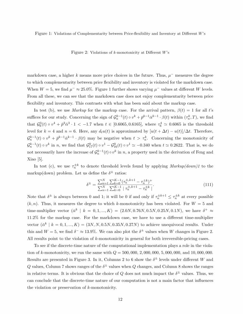
Figure 1: Violations of Complementarity between Price-flexibility and Inventory at Different W ’s

Figure 2: Violations of k-monotonicity at Different W ’s

markdown case, a higher k means more price choices in the future. Thus, µ− measures the degree

to which complementarity between price flexibility and inventory is violated for the markdown case.

When W = 5, we find µ− ≈ 25.0%. Figure 1 further shows varying µ− values at different W levels.

From all these, we can see that the markdown case does not enjoy complementarity between price

flexibility and inventory. This contrasts with what has been said about the markup case.

In test (b), we use Markup for the markup case. For the arrival pattern, β(t) = 1 for all t’s

suffices for our study. Concerning the sign of Gk−1n (t) vk + pk−1αk−1 · β(t) within (τkn , T ), we find

that G36(t) v4 + p3α3 · 1 < −1.7 when t ∈ [0.6065, 0.6165], where τ4

6 ' 0.6065 is the threshold

level for k = 4 and n = 6. Here, any dtu(t) is approximated by [u(t + ∆t) − u(t)]/∆t. Therefore,

Gk−1n (t) vk + pk−1αk−1 · β(t) may be negative when t > τkn . Concerning the monotonicity of

Gk−1n (t) vk in n, we find that G0

17(t) v1 − G016(t) v1 ' −0.340 when t ' 0.2622. That is, we do

not necessarily have the increase of Gk−1n (t) vk in n, a property used in the derivation of Feng and

Xiao [5].

In test (c), we use τ±kn to denote threshold levels found by applying Markup(down)1 to the

markup(down) problem. Let us define the δ± ratios:

δ± =

∑Nn=1

∑K−1k=0 (τ±,k+1

n − τ±kn )+∑Nn=1

∑K−1k=0 | τ

±,k+1n − τ±kn |

. (111)

Note that δ± is always between 0 and 1; it will be 0 if and only if τ±k+1n ≤ τ±kn at every possible

(k, n). Thus, it measures the degree to which k-monotonicity has been violated. For W = 5 and

time-multiplier vector (αk | k = 0, 1, ...,K) = (2.0N, 0.76N, 0.5N, 0.25N, 0.1N), we have δ+ ≈11.2% for the markup case. For the markdown case, we have to use a different time-multiplier

vector (αk | k = 0, 1, ...,K) = (3N,N, 0.5N, 0.35N, 0.27N) to achieve unequivocal results. Under

this and W = 5, we find δ− ≈ 13.9%. We can also plot the δ± values when W changes in Figure 2.

All results point to the violation of k-monotonicity in general for both irreversible-pricing cases.

To see if the discrete-time nature of the computational implementation plays a role in the viola-

tion of k-monotonicity, we run the same with Q = 500, 000, 2, 000, 000, 5, 000, 000, and 10, 000, 000.

Results are presented in Figure 3. In it, Columns 2 to 6 show the δ± levels under different W and

Q values, Column 7 shows ranges of the δ± values when Q changes, and Column 8 shows the ranges

in relative terms. It is obvious that the choice of Q does not much impact the δ± values. Thus, we

can conclude that the discrete-time nature of our computation is not a main factor that influences

the violation or preservation of k-monotonicity.

12

Figure 3: Violations of k-monotonicity when Q and W change

Figure 4: Benefits of Heeding Demand’s Time-variability at Different W ’s

In test (d), we suppose that, when not aware of the time-variability of β(·), the firm will take

the flat β′(t) = 1 as β(t) in its policy derivation. Let us use v+knq and τ+k

n to denote, respectively, the

values and threshold levels resulting from applying Markup to the markup problem defined by β(·),and use τ+′k

n to denote the threshold levels resulting from applying Markup to the corresponding

flat-rate problem defined by β′(·). To find the values v+′knq from applying the sub-optimal policy

defined by the τ+′kn ’s to the actual situation defined by β(·), we shall use algorithm Markup3.

Corresponding to Markup3, we have algorithms Markdown3 and Reversible3 for the markdown

and reversible-pricing cases, respectively. All these newly mentioned algorithms are described in

the end. For the markdown case, the relevant values will be denoted by v−knq and v−′knq , while for the

reversible-pricing case, these values will be denoted by v0nq and v0′

nq.

To measure the losses due to neglecting the time-variability of β(·), we may define η±(0) for the

markup(down) and reversible-pricing cases:

η± =

∑Kk=0(v±kN0 − v

±′kN0 )∑K

k=0 v±kN0

, η0 =v0N0 − v0′

N0

v0N0

. (112)

When W = 5, we have η+ ≈ 2.0%, η− ≈ 18.9%, and η0 ≈ 15.8%. Hence, the benefit of heeding

demand’s time-variability in each of the three cases is substantial. When W varies, we show the

η±(0) values in Figure 4. It is quite clear from the figure that the benefit increases with the degree

of the fluctuation.

In test (e), we abandon the product-form arrival pattern λk(t) = αk · β(t). In its stead, we let

λk(t) = αk · [1 + 0.8 · sin(2π · ( k0.3

+ t))]. (113)

Note that (113) is not defined by one single β(·) across different k values. As algorithms Markup,

Markdown, and Reversible are designed for cases where the arrival pattern is of the product form,

they are not guaranteed to arrive to correct answers any more. Indeed, discrepancies appear for the

current arrival pattern between results produced by these algorithms and those by the brute-force

algorithms. In Figure 5, we demonstrate the pricing decisions reached by Markup2 and Markdown2,

as well as pn(t) reached by Reversible2 at particular (k and) n values.

Since none of the above pricing decisions is decreasing in t, we simply can not define τkn for

any of these cases. Therefore, predictions made in the paper stop at the product-form case for

the time being. Note that λk+1(t)/λk(t) under (113) is not decreasing in t. Therefore, Zhao and

13

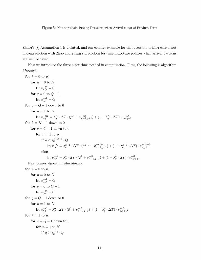
Figure 5: Non-threshold Pricing Decisions when Arrival is not of Product Form

Zheng’s [8] Assumption 1 is violated, and our counter example for the reversible-pricing case is not

in contradiction with Zhao and Zheng’s prediction for time-monotone policies when arrival patterns

are well behaved.

Now we introduce the three algorithms needed in computation. First, the following is algorithm

Markup3.

for k = 0 to K

for n = 0 to N

let v+′knQ = 0;

for q = 0 to Q− 1

let v+′k0q = 0;

for q = Q− 1 down to 0

for n = 1 to N

let v+′Knq = λKq ·∆T · (pK + v+′K

n−1,q+1) + (1− λKq ·∆T ) · v+′Kn,q+1;

for k = K − 1 down to 0

for q = Q− 1 down to 0

for n = 1 to N

if q < τ+′,k+1n ·Q

let v+′knq = λk+1

q ·∆T · (pk+1 + v+′,k+1n−1,q+1) + (1− λk+1

q ·∆T ) · v+′,k+1n,q+1 ;

else

let v+′knq = λkq ·∆T · (pk + v+′k

n−1,q+1) + (1− λkq ·∆T ) · v+′kn,q+1.

Next comes algorithm Markdown3.

for k = 0 to K

for n = 0 to N

let v−′knQ = 0;

for q = 0 to Q− 1

let v−′k0q = 0;

for q = Q− 1 down to 0

for n = 1 to N

let v−′0nq = λ0q ·∆T · (p0 + v−′0n−1,q+1) + (1− λ0

q ·∆T ) · v−′0n,q+1;

for k = 1 to K

for q = Q− 1 down to 0

for n = 1 to N

if q ≥ τ−′kn ·Q

14

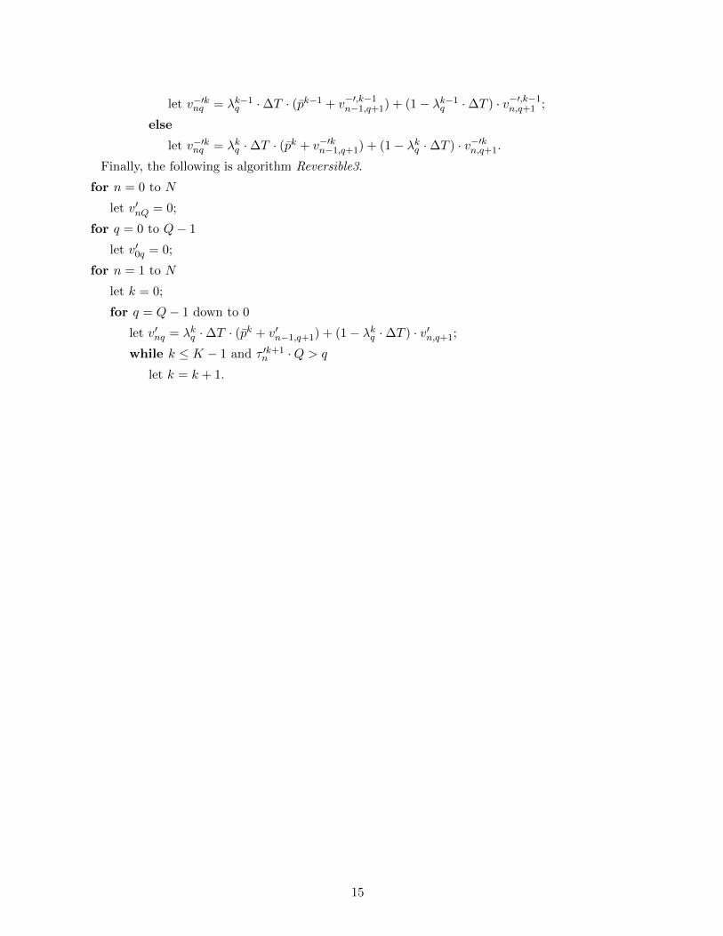
let v−′knq = λk−1q ·∆T · (pk−1 + v−′,k−1

n−1,q+1) + (1− λk−1q ·∆T ) · v−′,k−1

n,q+1 ;

else

let v−′knq = λkq ·∆T · (pk + v−′kn−1,q+1) + (1− λkq ·∆T ) · v−′kn,q+1.

Finally, the following is algorithm Reversible3.

for n = 0 to N

let v′nQ = 0;

for q = 0 to Q− 1

let v′0q = 0;

for n = 1 to N

let k = 0;

for q = Q− 1 down to 0

let v′nq = λkq ·∆T · (pk + v′n−1,q+1) + (1− λkq ·∆T ) · v′n,q+1;

while k ≤ K − 1 and τ ′k+1n ·Q > q

let k = k + 1.

15