Journal of Computational Physics 261 (2014) 83–105

Contents lists available at ScienceDirect

Journal of Computational Physics

www.elsevier.com/locate/jcp

A robust and accurate outflow boundary condition forincompressible flow simulations on severely-truncatedunbounded domains

S. Dong a,∗, G.E. Karniadakis b, C. Chryssostomidis c

a Department of Mathematics, Purdue University, United Statesb Division of Applied Mathematics, Brown University, United Statesc Department of Mechanical Engineering, Massachusetts Institute of Technology, United States

a r t i c l e i n f o a b s t r a c t

Article history:Received 29 June 2013Received in revised form 17 December 2013Accepted 19 December 2013Available online 3 January 2014

Keywords:OutflowBoundary conditionUnbounded domainHigh Reynolds numberSpectral element

We present a robust and accurate outflow boundary condition and an associated numericalalgorithm for incompressible flow simulations on unbounded physical domains, aimingat maximizing the domain truncation without adversely affecting the flow physics.The proposed outflow boundary condition allows for the influx of kinetic energy intothe domain through the outflow boundaries, and prevents un-controlled growth in theenergy of the domain in such situations. The numerical algorithm for the outflowboundary condition is developed on top of a rotational velocity-correction type strategyto de-couple the pressure and velocity computations, and a special construction in thealgorithmic formulation prevents the numerical locking at the outflow boundaries fortime-dependent problems. Extensive numerical tests for flow problems with bounded andsemi-bounded physical domains demonstrate that this outflow boundary condition and thenumerical algorithm produce stable and accurate simulations on even severely truncatedcomputational domains, where strong vortices may be present at or exit the outflowboundaries. The method developed herein has the potential to significantly expeditesimulations of incompressible flows involving outflow or open boundaries, and to enablesuch simulations at Reynolds numbers significantly higher than the state of the art.

© 2013 Elsevier Inc. All rights reserved.

1. Introduction

Outflows, or more generally open portions of the boundary, where the field variables are unknown and need to becomputed, are encountered in wakes, jets, boundary layers, arterial trees, and many other flow problems. How to deal withoutflows for incompressible flow simulations is a challenging and open issue. On the one hand, an ideal method wouldallow the flow and any information carried with it to exit the domain without adverse upstream effects [46]. On the otherhand, it should allow for stable computations regardless of the location of the outflow boundary, even at high Reynoldsnumbers. Simple analysis for a one-dimensional advection–diffusion system with the standard Neumann outflow conditionshows that, to maintain good solution accuracy, the length of the domain should scale linearly with the Reynolds or Pecletnumber, which is obviously a severe limitation.

* Corresponding author.E-mail address: sdong@math.purdue.edu (S. Dong).

0021-9991/$ – see front matter © 2013 Elsevier Inc. All rights reserved.http://dx.doi.org/10.1016/j.jcp.2013.12.042

84 S. Dong et al. / Journal of Computational Physics 261 (2014) 83–105

We briefly summarize the existing work on the outflow or open flows in the literature, restricting our attention toincompressible flows. For the outflow issues with compressible flows, some recent reviews are [3,15]; see also the referencestherein. For more general problems one can refer to [52] for a comprehensive review.

Given the importance of this topic, it is not surprising that a large volume of literature exists on the outflow conditionsfor incompressible flows. The techniques for dealing with outflow boundaries have been reviewed, up to the mid-1990s, in[46]; see also [17] and the references therein. The types and the ease in implementation of the outflow boundary condi-tions are closely associated with the spatial discretization schemes. The traction-free boundary condition (or its variants, e.g.no-flux condition) at the outflow is one of the most commonly used [50,14,10,33,1,46,2,21,34], especially for finite element-type discretizations. The convective (or radiation) boundary condition (see e.g. [39,17,30,38,11,45]) has often been used withfinite difference or finite volume type discretizations.

A number of other types of outflow conditions have been proposed based on various strategies over the years. In [26]a non-reflecting condition was developed through a factorization of the wave operator and by making an analogy betweenthe incompressible Navier–Stokes equation and the factorized wave equation. A free boundary condition at the outflowwas proposed in [40], where the unknown surface integral term at the outflow boundary in the weak formulation of theNavier–Stokes equation was moved back to the left hand side and incorporated into the coefficient matrix. This is oftenreferred to as “do-nothing” boundary condition or “no-boundary-condition” condition. This boundary condition has beenanalyzed in [19,43], and it is equivalent to imposing the condition that the (N + 1)-st derivative of the field variable,where N is the polynomial degree of the finite elements, should vanish at a point near the outflow boundary. Anotheroutflow condition, which was proposed in [27] and aims to suppress a boundary layer at the open boundary, requiresa normal derivative of a high order of some independent variable to vanish at the outflow boundary. In the method of[23], the velocity at the outflow boundary is determined by extrapolating the velocity from the interior of domain and byutilizing an asymptotic velocity field at infinity, while the pressure at the outflow boundary is determined by using thetraction-free condition. In [35], a velocity–pressure formulation of the Navier–Stokes equations was used, where a pressurePoisson equation replaces the velocity divergence-free condition (see also e.g. [17,34]), and then a set of conditions for boththe outflow and inflow boundaries are obtained by solving an eigen-value problem at the boundaries [36]. An augmentedLagrangian method was developed in [31], where the velocity profiles at the outflow boundaries are constrained to achievecertain desired properties. In [42,41], an equation for the pressure at the outflow boundary is derived involving derivativesalong the tangential direction of the outflow boundary. It is then proposed that the pressure condition at the outflowboundary be determined by solving this equation. Defective boundary conditions, in which only the averaged quantities suchas the flow rate or pressure drop are available on portions of the domain boundary, are important for many applicationssuch as blood flow simulations in arterial networks [20]. This type of problems has been considered in [24]; see also [12].

In production simulations a common observation with outflows is that, especially at high and moderate Reynolds num-bers (or even at low Reynolds numbers in certain situations), the computation would become unstable when strong vorticesare present at or exit the outflow boundaries [6,7]. Owing to the lack of effective techniques, a usual remedy for thisproblem is to employ a large computational domain, e.g. by placing the outflow boundary far away from the domain ofinterest, such that the presence of outflow boundary would not significantly disturb the flow, and more importantly, thevortices generated upstream would be sufficiently dissipated before reaching the outflow boundary. For example, in thethree-dimensional direct numerical simulation of turbulent flow past a circular cylinder at Reynolds number Re = 10,000[7], a wake region of length 50D (D being the cylinder diameter) in the streamwise direction has been employed. Eventhough the far-wake region was not of interest in that study, such a large computational domain is essential for numer-ical stability in order for the vortices to be sufficiently dissipated before reaching the outflow boundary at that Reynoldsnumber. This practice has several drawbacks: the large computational domain requires a large mesh and induces a largecomputational cost, and much of the grid resolution would be wasted in the far regions which are of little or no physicalinterest. In addition, this strategy is not scalable with respect to the Reynolds number [7].

In this paper, we present a robust and accurate outflow boundary condition, and the associated numerical algorithm,that allow for stable simulations of incompressible flows on even severely truncated computational domains, where strongvortices may be present at or exit the outflow boundaries. Fig. 1 shows a snapshot of the instantaneous velocity fieldand pressure distribution (color contours) of the flow past a square cylinder at Reynolds number Re = 10,000 from atwo-dimensional (2-D) simulation using our method. The computational domain has a streamwise length of only 5.5D inthe cylinder wake, where D is the cylinder dimension. One can clearly observe the strong vortices passing through theoutflow boundary. The new outflow boundary condition is designed in such a fashion that the influx of kinetic energy intothe domain through the outflow boundaries, if any, will not cause un-controlled growth in the energy of the domain. Thealgorithm for dealing with this outflow boundary condition is developed on top of a rotational velocity-correction typestrategy [8] for de-coupling the pressure and velocity computations in the incompressible Navier–Stokes equations. In thepressure and velocity sub-steps, different types of discrete conditions are imposed for the pressure and the velocity on theoutflow boundaries. A special construction in the algorithmic formulation obviates the numerical locking on the outflowboundaries for time-dependent problems.

The method developed herein can potentially enable the use of a much smaller computational domain for incompressibleflow simulations at high Reynolds numbers. With the current method the domain size will only be restricted by considera-tions of physical accuracy, not by the numerical stability associated with the outflow boundary. Since one can pack all the

S. Dong et al. / Journal of Computational Physics 261 (2014) 83–105 85

Fig. 1. (Color online.) Instantaneous velocity field and pressure contours (in color) of the flow past a square cylinder at Re = 10,000. The wake region hasa length 5.5D in streamwise direction, where D is the cylinder dimension. Velocity vectors are plotted on every fourth quadrature point in each directionwithin each element.

grid resolution into a small computational domain, flow regimes at Reynolds numbers much higher than the current stateof the art can potentially be reached more easily using this technique.

2. Outflow boundary condition and algorithm

2.1. New outflow boundary condition

Let Ω denote an open bounded domain in two or three dimensions, and ∂Ω denote its boundary. We consider theappropriately-normalized incompressible Navier–Stokes equations on Ω ,

∂u

∂t+ u · ∇u = −∇p + ν∇2u + f, (1a)

∇ · u = 0, (1b)

where u(x, t) is velocity, p(x, t) is pressure, f(x, t) is an external body force, and x and t are respectively the spatial coordi-nate and time. The non-dimensional viscosity is ν = 1

Re , where Re is the Reynolds number defined by appropriately choosingthe characteristic velocity and length scales; we assume that the fluid density is ρ = 1.

We assume ∂Ω = ∂Ωd ∪ ∂Ωo , where on ∂Ωd the velocity u is prescribed while on ∂Ωo neither u nor p is known. Wewill refer to ∂Ωo as the outflow boundary hereafter. Eqs. (1a) and (1b) are supplemented by the boundary condition,

u = w(x, t), on ∂Ωd, (2)

where w is the prescribed boundary velocity on ∂Ωd .We propose the following boundary condition for ∂Ωo ,

−pn + νn · ∇u −[

1

2|u|2 S0(n · u)

]n = fb(x, t), on ∂Ωo, (3)

where n is the outward-pointing unit vector normal to ∂Ωo , and |u| denotes the magnitude of velocity u. fb is a vectorfunction on ∂Ωo for the purpose of numerical testing only, and it is set to zero in actual simulations. The scalar functionS0(n · u) is given by

S0(n · u) = 1

2

(1 − tanh

n · u

U0δ

), (4)

where U0 is the characteristic velocity scale, and δ > 0 is a chosen non-dimensional positive constant that is sufficientlysmall. When the value δ approaches zero, the function S0 becomes the step function about (n · u). So S0(n · u) representsa smoothed step function, taking essentially unit value in regions where n · u < 0 and vanishing elsewhere. δ controls thesharpness of the smoothed step function, and it is sharper when δ is smaller. Numerical tests (see Section 3.2) show thatwhen δ is small the simulation result is not sensitive to its value.

The boundary condition (3) has a well-defined physical meaning when fb = 0. The term − 12 |u|2n represents an effective

stress exerting on ∂Ωo induced by the influx of kinetic energy into the domain Ω through ∂Ωo . The terms (−pn + νn · ∇u)represents the stress on ∂Ωo . Therefore, the condition (3) with fb = 0 imposes the requirement that, if anywhere on ∂Ωothere is an energy influx into domain through ∂Ωo then the stress on ∂Ωo shall locally balance the effective stress inducedby the energy influx, otherwise the stress shall locally be zero.

One can more clearly understand the above condition by considering the energy balance equation for the system (1a)and (1b). By taking the L2 inner product between u and Eq. (1a) and using Eq. (1b), one gets the following energy equation,

86 S. Dong et al. / Journal of Computational Physics 261 (2014) 83–105

∂

∂t

∫Ω

1

2|u|2 = −ν

∫Ω

‖∇u‖2 +∫Ω

f · u +∫

∂Ωd

(n · T − 1

2|u|2n

)· u +

∫∂Ωo

(n · T − 1

2|u|2n

)· u, (5)

where T = −pI + ν∇u (I denotes the identity tensor). The last term on the right hand side (RHS) of the above equation,i.e. the surface integral over ∂Ωo , can potentially cause un-controlled energy growth in the domain, and thus numericalinstability, if n ·u < 0 anywhere on ∂Ωo , because of the energy influx − 1

2 |u|2(n ·u). Imposing the condition n ·T− 12 |u|2n = 0

in regions with energy influx on ∂Ωo will eliminate this instability. On the other hand, on a Dirichlet boundary ∂Ωd becauseu is prescribed, the energy influx through ∂Ωd (if any) will not create the numerical instability issue.

In addition to the boundary conditions (2) and (3), appropriate initial conditions for the velocity u will also need to bespecified.

If a stress-divergence form, ν∇ · (∇u +∇uT ), is used for the viscous term in the Navier–Stokes equation (1a), the outflowboundary condition will be modified accordingly,

−pn + νn · (∇u + ∇uT ) −[

1

2|u|2 S0(n · u)

]n = fb(x, t), on ∂Ωo. (6)

2.2. Numerical algorithm and implementation

Eqs. (1a) and (1b), the boundary conditions (2) and (3), and the appropriate initial condition for the velocity togetherconstitute the system that needs to be solved in flow simulations. Next, we present an algorithm for solving this system.Our emphasis is on how to numerically treat the outflow boundary condition (3).

Let un and pn denote the velocity and pressure at time step n. To compute these variables at time step (n + 1), wesuccessively solve for the pressure and the velocity as follows:

For pressure pn+1:γ0un+1 − u

�t+ un · ∇un + ∇pn+1 + ν∇ × ∇ × un = fn+1, (7a)

∇ · un+1 = 0, (7b)

n · un+1 = n · wn+1, on ∂Ωd, (7c)

pn+1 = νn · ∇u∗,n+1 · n − 1

2

∣∣u∗,n+1∣∣2

S0(n · u∗,n+1) − fn+1

b · n, on ∂Ωo. (7d)

For velocity un+1:γ0un+1 − γ0un+1

�t− ν∇2un+1 + u∗,n+1 · ∇u∗,n+1 = un · ∇un + ν∇ × ∇ × un, (8a)

un+1 = wn+1 on ∂Ωd, (8b)

n · ∇un+1 = 1

ν

[pn+1n + 1

2

∣∣u∗,n+1∣∣2

S0(n · u∗,n+1)n − ν

(∇ · u∗,n+1)n + fn+1b

], on ∂Ωo. (8c)

In the above equations, �t is the time step size, and n is the outward-pointing unit vector normal to ∂Ω; un+1 denotesan intermediate velocity, which is an approximation of un+1. The time derivative ∂u

∂t is approximated at time step (n + 1)by a J -th order ( J = 1 or 2) backward differentiation formula (BDF) [5], that is,

γ0 ={

1, if J = 1,32 , if J = 2,

u ={

un, if J = 1,

2un − 12 un−1, if J = 2.

(9)

The variable u∗,n+1 represents a J -th order explicit approximation of un+1 as follows,

u∗,n+1 ={

un, if J = 1,

2un − un−1, if J = 2.(10)

fn+1 and fn+1b respectively represent f(x, t) and fb(x, t) at time step (n + 1).

One can observe that this scheme employs an overall rotational velocity-correction type strategy (see [22,8]) to de-couplethe computations for the pressure and the velocity. For the pressure step, on the outflow boundary ∂Ωo a pressure Dirichletcondition (7d) has been imposed, which is obtained by taking the inner product between the outflow boundary condition (3)and n, and the velocity involved in (7d) has been treated explicitly. For the velocity step, on the outflow boundary ∂Ωo avelocity Neumann-type condition (8c), which stems essentially from the outflow boundary condition (3), has been imposed.However, this velocity Neumann condition (8c) contains an extra term in the construction, (∇ · u∗,n+1)n. This construction

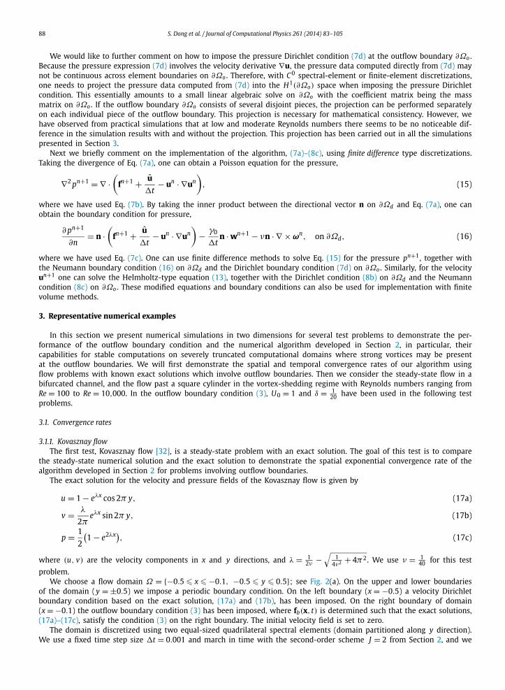
S. Dong et al. / Journal of Computational Physics 261 (2014) 83–105 87

is crucial to the scheme. If this term is absent, then by combining (7d) and (8c) and assuming fb = 0, one can show thatn · ∇un+1|∂Ωo = n · ∇un|∂Ωo = · · · = n · ∇u1|∂Ωo = (n · ∇u0 · n)n|∂Ωo , leading to a numerical locking at the outflow boundary∂Ωo for time-dependent problems.

We would like to comment on the treatments of the non-linear term and the viscous term (in rotational form) in (7a)of the pressure step. Both terms are approximated at time step n, instead of at time step (n + 1) like the rest of the terms.These treatments do not compromise the temporal accuracy of the velocity because of the correction terms in Eq. (8a),u∗,n+1 · ∇u∗,n+1 − un · ∇un , and −ν∇2un+1 − ν∇ ×∇ × un . The analysis in [22] for the Stokes equation (no non-linear term)indicates that this type of treatment may slightly decrease the temporal accuracy of the pressure for certain error norms.However, this effect on the pressure seems not noticeable in our numerical experiments; see Section 3.1. Alternatively, onecan also approximate the nonlinear term and the viscous term (in rotational form) explicitly at time step (n +1) in (7a), andaccordingly Eq. (8a) will need to be modified to remove the correction terms. Such a treatment has been discussed in [9](Section 2.5 of that reference) in the context of variable-density Navier–Stokes equations.

Next we re-formulate the algorithm, (7a)–(8c), in order to facilitate the implementation with C0 spectral elements andfinite elements. We will eliminate the intermediate velocity u from the formulation, and also appropriately treat the second-derivative term ∇ × ∇ × u, which cannot be computed directly with C0 elements.

Let H1a0(Ω) = {v ∈ H1(Ω): v|∂Ωo = 0}, and q ∈ H1

a0(Ω) denote the test function. Taking the L2 inner product betweenEq. (7a) and ∇q, we can obtain the following pressure weak form,∫

Ω

∇pn+1 · ∇q =∫Ω

(fn+1 + u

�t− un · ∇un

)· ∇q − ν

∫∂Ωd

n × ωn · ∇q − ν

∫∂Ωo

n × ωn · ∇q

− γ0

�t

∫∂Ωd

n · wn+1q, ∀q ∈ H1a0(Ω), (11)

where ω = ∇ × u is the vorticity, and we have used Eqs. (7b) and (7c), and the identity ∇ ×ω · ∇q = ∇ · (ω × ∇q). We havealso used the fact that

∫∂Ωo

n · un+1q = 0 because q ∈ H1a0(Ω).

The intermediate velocity un+1, according to (7a), is given by

un+1 = �t

γ0

(fn+1 + u

�t− un · ∇un − ∇pn+1 − ν∇ × ωn

). (12)

Substituting this expression into (8a), and one can get

γ0

ν�tun+1 − ∇2un+1 = 1

ν

(fn+1 + u

�t− u∗,n+1 · ∇u∗,n+1 − ∇pn+1

). (13)

Let H10(Ω) = {v ∈ H1(Ω): v|∂Ωd = 0}, and φ ∈ H1

0(Ω) denote the test function. Taking the L2 inner product betweenEq. (13) and φ, we can obtain the following weak form for the velocity,

γ0

ν�t

∫Ω

φun+1 +∫Ω

∇φ · ∇un+1 = 1

ν

∫Ω

(fn+1 + u

�t− u∗,n+1 · ∇u∗,n+1 − ∇pn+1

)φ

+ 1

ν

∫∂Ωo

[pn+1n + 1

2

∣∣u∗,n+1∣∣2

S0(n · u∗,n+1)n − ν

(∇ · u∗,n+1)n + fn+1b

]φ, ∀φ ∈ H1

0(Ω), (14)

where we have used Eq. (8c) and the fact that∫∂Ωd

n · ∇un+1φ = 0 because φ ∈ H10(Ω).

Therefore, the re-formulated algorithm is as follows: Given (un, pn), we successively solve for pn+1 and un+1 in twosteps:

1. Solve Eq. (11), together with the pressure Dirichlet condition (7d) on ∂Ωo , for pn+1;2. Solve Eq. (14), together with the velocity Dirichlet condition (8b) on ∂Ωd , for un+1.

We note the following characteristics of this algorithm:

• The intermediate velocity un+1 is eliminated;• No derivative of order two or higher is involved and thus C0 spectral elements or finite elements can be directly used;• Different components of the velocity un+1 are not coupled in Eq. (14), and can therefore be computed individually.

Eqs. (11) and (14) are in weak forms, and therefore can be discretized in space with spectral elements or finite elementsin a straightforward fashion. We have employed spectral element spatial discretizations [28,53] in the current paper.

88 S. Dong et al. / Journal of Computational Physics 261 (2014) 83–105

We would like to further comment on how to impose the pressure Dirichlet condition (7d) at the outflow boundary ∂Ωo .Because the pressure expression (7d) involves the velocity derivative ∇u, the pressure data computed directly from (7d) maynot be continuous across element boundaries on ∂Ωo . Therefore, with C0 spectral-element or finite-element discretizations,one needs to project the pressure data computed from (7d) into the H1(∂Ωo) space when imposing the pressure Dirichletcondition. This essentially amounts to a small linear algebraic solve on ∂Ωo with the coefficient matrix being the massmatrix on ∂Ωo . If the outflow boundary ∂Ωo consists of several disjoint pieces, the projection can be performed separatelyon each individual piece of the outflow boundary. This projection is necessary for mathematical consistency. However, wehave observed from practical simulations that at low and moderate Reynolds numbers there seems to be no noticeable dif-ference in the simulation results with and without the projection. This projection has been carried out in all the simulationspresented in Section 3.

Next we briefly comment on the implementation of the algorithm, (7a)–(8c), using finite difference type discretizations.Taking the divergence of Eq. (7a), one can obtain a Poisson equation for the pressure,

∇2 pn+1 = ∇ ·(

fn+1 + u

�t− un · ∇un

), (15)

where we have used Eq. (7b). By taking the inner product between the directional vector n on ∂Ωd and Eq. (7a), one canobtain the boundary condition for pressure,

∂ pn+1

∂n= n ·

(fn+1 + u

�t− un · ∇un

)− γ0

�tn · wn+1 − νn · ∇ × ωn, on ∂Ωd, (16)

where we have used Eq. (7c). One can use finite difference methods to solve Eq. (15) for the pressure pn+1, together withthe Neumann boundary condition (16) on ∂Ωd and the Dirichlet boundary condition (7d) on ∂Ωo . Similarly, for the velocityun+1 one can solve the Helmholtz-type equation (13), together with the Dirichlet condition (8b) on ∂Ωd and the Neumanncondition (8c) on ∂Ωo . These modified equations and boundary conditions can also be used for implementation with finitevolume methods.

3. Representative numerical examples

In this section we present numerical simulations in two dimensions for several test problems to demonstrate the per-formance of the outflow boundary condition and the numerical algorithm developed in Section 2, in particular, theircapabilities for stable computations on severely truncated computational domains where strong vortices may be presentat the outflow boundaries. We will first demonstrate the spatial and temporal convergence rates of our algorithm usingflow problems with known exact solutions which involve outflow boundaries. Then we consider the steady-state flow in abifurcated channel, and the flow past a square cylinder in the vortex-shedding regime with Reynolds numbers ranging fromRe = 100 to Re = 10,000. In the outflow boundary condition (3), U0 = 1 and δ = 1

20 have been used in the following testproblems.

3.1. Convergence rates

3.1.1. Kovasznay flowThe first test, Kovasznay flow [32], is a steady-state problem with an exact solution. The goal of this test is to compare

the steady-state numerical solution and the exact solution to demonstrate the spatial exponential convergence rate of thealgorithm developed in Section 2 for problems involving outflow boundaries.

The exact solution for the velocity and pressure fields of the Kovasznay flow is given by

u = 1 − eλx cos 2π y, (17a)

v = λ

2πeλx sin 2π y, (17b)

p = 1

2

(1 − e2λx), (17c)

where (u, v) are the velocity components in x and y directions, and λ = 12ν −

√1

4ν2 + 4π2. We use ν = 140 for this test

problem.We choose a flow domain Ω = {−0.5 � x � −0.1, −0.5 � y � 0.5}; see Fig. 2(a). On the upper and lower boundaries

of the domain (y = ±0.5) we impose a periodic boundary condition. On the left boundary (x = −0.5) a velocity Dirichletboundary condition based on the exact solution, (17a) and (17b), has been imposed. On the right boundary of domain(x = −0.1) the outflow boundary condition (3) has been imposed, where fb(x, t) is determined such that the exact solutions,(17a)–(17c), satisfy the condition (3) on the right boundary. The initial velocity field is set to zero.

The domain is discretized using two equal-sized quadrilateral spectral elements (domain partitioned along y direction).We use a fixed time step size �t = 0.001 and march in time with the second-order scheme J = 2 from Section 2, and we

S. Dong et al. / Journal of Computational Physics 261 (2014) 83–105 89

Fig. 2. Kovasznay flow (steady-state problem): (a) streamlines; (b) L∞ and L2 errors of numerical solution versus element order showing exponentialconvergence rate, computed on two quadrilateral elements. Outflow condition is imposed on the right boundary of domain.

Fig. 3. Kovasznay flow: Numerical errors versus element order, with fb = 0 in the outflow boundary condition (3). (a) L∞ and L2 errors for different flowvariables obtained on a domain with dimension in the x direction: x ∈ [−0.5,5.0]. (b) L2 errors of the x velocity component obtained on domains withdifferent dimensions in the x direction.

vary the element order systematically. After the steady state is reached, we compute the errors in different norms betweenthe steady-state numerical solution and the exact solution (17a)–(17c).

Fig. 2(a) demonstrates the flow pattern of the steady-state field using the streamlines. In Fig. 2(b) we plot the L∞ andL2 errors of the velocity components and the pressure from the numerical solution as a function of the element order. Thenumerical errors decrease exponentially as the element order increases. The results demonstrate the spatial exponentialconvergence rate of our algorithm for steady-state problem involving the outflow boundary condition (3).

We have also performed another set of tests, in which we set fb = 0 in the outflow boundary condition (3) to mimicreal flow situations where the true fb is unknown. This error on the outflow boundary will ultimately dominate the errorsin the numerical solution when the mesh resolution increases, and the numerical errors will be saturated by it. This isdemonstrated by Fig. 3. Fig. 3(a) shows the L∞ and L2 errors of the velocity and the pressure as a function of the elementorder obtained on a domain with a dimension in the x direction −0.5 � x � 5.0, and Fig. 3(b) shows the L2 errors of the xvelocity component versus element order obtained on several domains with different dimensions in the x direction (locationof the right boundary ranges from −0.1 to 5.0). The domain dimension in the y direction has been fixed at −0.5 � y � 0.5.It is evident that the numerical errors decrease exponentially with increasing element order until the saturation by theerror at the outflow boundary. On the domain −0.5 � x � −0.1 (same as that of Fig. 2), the numerical error is saturatedat a level about 10−2, and on the domain −0.5 � x � 5.0, the error is saturated at a level about 10−5. Note that, becausethe pressure can only be determined uniquely up to an arbitrary additive constant, in this set of tests (with fb = 0) for

90 S. Dong et al. / Journal of Computational Physics 261 (2014) 83–105

comparison we have shifted the exact pressure solution (17c) by a constant as follows, such that the exact pressure valueat the right boundary is zero,

p = 1

2

(1 − e2λx) − 1

2

(1 − e2λL),

where x = L is the coordinate of the right domain boundary.Given that exponential convergence is very sensitive to any inconsistent modeling errors, this example demonstrates the

accuracy and consistency of the new outflow boundary condition.

3.1.2. Time-dependent problemWe next consider an unsteady flow with a contrived analytic solution. The goal of this test is to demonstrate the spatial

and temporal convergence rates of the algorithm developed in Section 2 for time-dependent problems involving outflowboundaries.

We consider the following analytic expressions for the velocity and pressure:

u = A sinαx cosπ y sinβt, (18a)

v = − Aα

πcosαx sinπ y sin βt, (18b)

p = A sinαx sinπ y cos βt (18c)

where A, α and β are prescribed constants. The velocity (u, v) expressions satisfy Eq. (1b). In the Navier–Stokes equa-tion (1a) the external body force f(x, t) is chosen such that the analytic expressions (18a)–(18c) satisfy Eq. (1a). Theparameters for this test problem are chosen as

ν = 0.01, A = 2, α = π, β = 1, ρ = 1.

We choose a computational domain Ω = {(x, y): 0 � x � 2, −1 � y � 1}, shown in Fig. 4(a) as ABC D . The domain ispartitioned along the x direction into two quadrilateral spectral elements of equal sizes, AE F D and E BC F . On the faces AB ,D F , and AD we impose the Dirichlet boundary condition for the velocity based on the analytic expressions (18a) and (18b).On the faces BC and C F we impose the outflow boundary condition (3), in which fb(x, t) is chosen such that the analyticexpressions (18a)–(18c) satisfy Eq. (3) on the outflow boundaries. The initial velocity field is set according to the analyticexpressions (18a) and (18b).

We employ the algorithm from Section 2, with J = 2 (temporal second order), and integrate the Navier–Stokes equationsin time from t = 0 to t = t f . Then we compute the errors of the numerical solutions at t = t f for different flow variablesagainst the analytic expressions given by (18a)–(18c).

In the first set of tests, we use a fixed small time step size �t = 0.001 and a fixed final integration time t f = 0.1 (100time steps). We vary the element order systematically, and for each element order we march in time to t = t f . Fig. 4(b)shows the L∞ and L2 errors of the velocity components and the pressure at t = t f between the numerical solution and theanalytic solution as a function of the element order. The spatial exponential convergence rate can be clearly observed forthe time-dependent problem.

In the second set of tests, we use a fixed large element order 18, and fix the final integration time at t f = 0.5. We varythe time step size systematically between �t = 0.003125 and �t = 0.1, and compute the errors of the numerical solutionat t = t f against the analytic solution. In Fig. 4(c) we plot the L∞ and L2 errors of the velocity and pressure as a functionof �t in logarithmic scales. The results show a temporal second-order convergence rate for the flow variables.

To summarize, for time-dependent problems involving outflow boundaries, the above results show that the algorithmdeveloped in Section 2 exhibits a temporal second-order convergence rate and a spatial exponential convergence rate.

3.2. Flow in a bifurcated channel

In this section we consider the flow in a bifurcated channel. The goal is to investigate the effects of the domain size andthe proposed outflow boundary condition on the steady-state flow field. This test problem was also used by several otherresearchers in previous studies; see e.g. [34,42].

The flow domain (see Fig. 5) is defined by Ω = [0, L] × [−0.5,0.5]\{[0,0.5] × [−0.5,0] ∪ [1.5, L] × [−0.1,0.2]}, whereall lengths are non-dimensionalized by a unit length. L > 1.5 is the size of the flow domain along the x direction, and ithas been varied in this study. The left boundary of the domain (x = 0) is the inlet, where a parabolic profile is imposed forthe x velocity component with a unit value at the inlet centerline (U0 = 1) and the y velocity component is set to zero.The outlets of the two bifurcations are located at the right boundary of the domain (x = L), where the outflow boundarycondition (3) has been imposed with fb = 0. No slip condition has been imposed on all the channel walls. The initial velocityfield is set to zero in the simulations.

We consider a Reynolds number Re = 600, based on the inlet centerline velocity and the unit length. The flow exhibitsa steady state at this Reynolds number; see the streamlines and pressure contours in Fig. 5. The density of the fluid isassumed to be ρ = 1.

S. Dong et al. / Journal of Computational Physics 261 (2014) 83–105 91

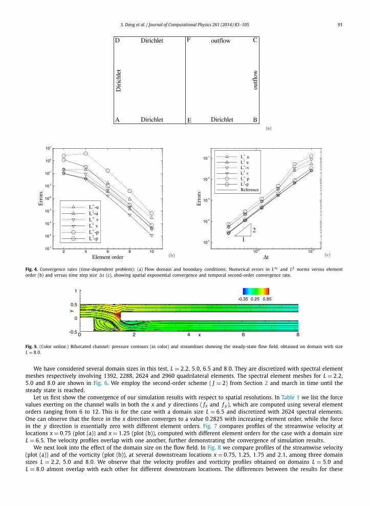
Fig. 4. Convergence rates (time-dependent problem): (a) Flow domain and boundary conditions; Numerical errors in L∞ and L2 norms versus elementorder (b) and versus time step size �t (c), showing spatial exponential convergence and temporal second-order convergence rate.

Fig. 5. (Color online.) Bifurcated channel: pressure contours (in color) and streamlines showing the steady-state flow field, obtained on domain with sizeL = 8.0.

We have considered several domain sizes in this test, L = 2.2, 5.0, 6.5 and 8.0. They are discretized with spectral elementmeshes respectively involving 1392, 2288, 2624 and 2960 quadrilateral elements. The spectral element meshes for L = 2.2,5.0 and 8.0 are shown in Fig. 6. We employ the second-order scheme ( J = 2) from Section 2 and march in time until thesteady state is reached.

Let us first show the convergence of our simulation results with respect to spatial resolutions. In Table 1 we list the forcevalues exerting on the channel walls in both the x and y directions ( fx and f y), which are computed using several elementorders ranging from 6 to 12. This is for the case with a domain size L = 6.5 and discretized with 2624 spectral elements.One can observe that the force in the x direction converges to a value 0.2825 with increasing element order, while the forcein the y direction is essentially zero with different element orders. Fig. 7 compares profiles of the streamwise velocity atlocations x = 0.75 (plot (a)) and x = 1.25 (plot (b)), computed with different element orders for the case with a domain sizeL = 6.5. The velocity profiles overlap with one another, further demonstrating the convergence of simulation results.

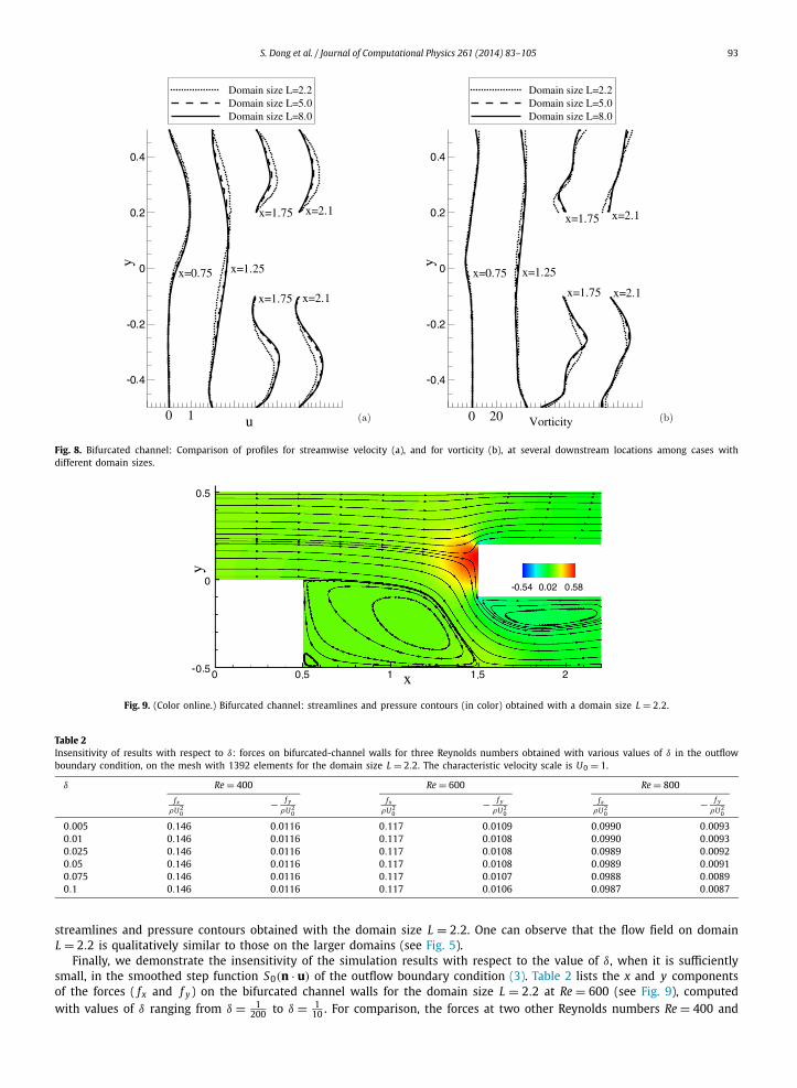
We next look into the effect of the domain size on the flow field. In Fig. 8 we compare profiles of the streamwise velocity(plot (a)) and of the vorticity (plot (b)), at several downstream locations x = 0.75, 1.25, 1.75 and 2.1, among three domainsizes L = 2.2, 5.0 and 8.0. We observe that the velocity profiles and vorticity profiles obtained on domains L = 5.0 andL = 8.0 almost overlap with each other for different downstream locations. The differences between the results for these

92 S. Dong et al. / Journal of Computational Physics 261 (2014) 83–105

Fig. 6. Spectral element meshes with (a) 1392, (b) 2288 and (c) 2960 quadrilateral elements for different domain sizes for the bifurcated channel.

Table 1Bifurcated channel: forces on channel walls obtained with various elementorders on the mesh with 2624 elements for the domain size L = 6.5.

Element order fx

ρU 20

f y

ρU 20

6 0.2834 8.4E−58 0.2826 8.9E−5

10 0.2825 7.7E−512 0.2825 6.8E−5

Fig. 7. Bifurcated channel: comparison of streamwise velocity profiles at locations (a) x = 0.75 and (b) x = 1.25 obtained with different element orders fordomain size L = 6.5, showing convergence of simulation results.

two cases are quite small. On the other hand, the velocity and vorticity profiles obtained on the smallest domain L = 2.2are qualitatively similar to, but exhibit a more pronounced quantitative difference from, those for domain sizes L = 8.0and L = 5.0. In the bulk of the lower bifurcation branch, the streamwise velocity obtained on the domain L = 2.2 appearsnotably smaller than those obtained on domains L = 5.0 and L = 8.0, while on the upper branch they appear notably larger.This difference is due to the “draconian” truncation of the domain with L = 2.2, where the outflow boundary cuts throughthe re-circulation bubble on the upper wall of the lower bifurcation branch. This is evident from Fig. 9, which shows the

S. Dong et al. / Journal of Computational Physics 261 (2014) 83–105 93

Fig. 8. Bifurcated channel: Comparison of profiles for streamwise velocity (a), and for vorticity (b), at several downstream locations among cases withdifferent domain sizes.

Fig. 9. (Color online.) Bifurcated channel: streamlines and pressure contours (in color) obtained with a domain size L = 2.2.

Table 2Insensitivity of results with respect to δ: forces on bifurcated-channel walls for three Reynolds numbers obtained with various values of δ in the outflowboundary condition, on the mesh with 1392 elements for the domain size L = 2.2. The characteristic velocity scale is U0 = 1.

δ Re = 400 Re = 600 Re = 800

fx

ρU 20

− f y

ρU 20

fx

ρU 20

− f y

ρU 20

fx

ρU 20

− f y

ρU 20

0.005 0.146 0.0116 0.117 0.0109 0.0990 0.00930.01 0.146 0.0116 0.117 0.0108 0.0990 0.00930.025 0.146 0.0116 0.117 0.0108 0.0989 0.00920.05 0.146 0.0116 0.117 0.0108 0.0989 0.00910.075 0.146 0.0116 0.117 0.0107 0.0988 0.00890.1 0.146 0.0116 0.117 0.0106 0.0987 0.0087

streamlines and pressure contours obtained with the domain size L = 2.2. One can observe that the flow field on domainL = 2.2 is qualitatively similar to those on the larger domains (see Fig. 5).

Finally, we demonstrate the insensitivity of the simulation results with respect to the value of δ, when it is sufficientlysmall, in the smoothed step function S0(n · u) of the outflow boundary condition (3). Table 2 lists the x and y componentsof the forces ( fx and f y) on the bifurcated channel walls for the domain size L = 2.2 at Re = 600 (see Fig. 9), computedwith values of δ ranging from δ = 1 to δ = 1 . For comparison, the forces at two other Reynolds numbers Re = 400 and

200 10

94 S. Dong et al. / Journal of Computational Physics 261 (2014) 83–105

Re = 800 have also been included in the table. One can observe that, for Re = 600 and Re = 400 different δ values result inidentical fx values, and for Re = 800 essentially the same fx values (difference ∼ 0.1%). The f y values at Re = 400 obtainedwith different δ are the same. At Re = 600 and Re = 800, the f y values computed with different δ are also essentially thesame (essentially zero), but some slight difference can be observed when δ decreases from 1

10 initially (about 1% or 2%). Itis evident that the simulation result is not sensitive to δ when it is sufficiently small.

3.3. Flow past a square cylinder

In this section we will consider the flow past a square cylinder, in two dimensions, at Reynolds numbers ranging fromRe = 100 to Re = 10,000. The flow is characterized by vortex shedding in the cylinder wake. At the higher Reynolds numbersconsidered here, in reality the flow will be three-dimensional and the wake will become turbulent. However, we will onlyconsider two-dimensional simulations here where the importance of outflow boundary condition is even more significantas two-dimensional vortices are typically stronger than their three-dimensional counterparts in this flow problem [6]. Ourgoals are: (1) to investigate the effects of domain sizes on the simulation results, and (2) to demonstrate the stability of theproposed outflow boundary condition and algorithm on highly truncated domains at moderate to high Reynolds numbers.

We consider a square cylinder occupying the region, − D2 � x � D

2 and − D2 � y � D

2 , where D = 1 is the dimension ofthe cylinder, and a flow domain, −5D � x � Lx and −L y � y � L y ; see Fig. 10. In the following tests, we vary the locationof the right domain boundary x = Lx in order to modify the streamwise extent of the cylinder wake region.

On the left domain boundary (x = −5D), a uniform flow comes into the domain, (u, v) = (U0,0), where U0 = 1 is thefree-stream velocity. On the upper and lower domain boundaries (x = ±L y ), we impose the periodic boundary condition.This configuration therefore corresponds more closely to the flow past an array of square cylinders aligned along the ydirection. On the right domain boundary (x = Lx), the outflow boundary condition (3) with fb = 0 will be imposed. We useδ = 1

20 in the function S0(n · u) (see Eq. (4)) in the simulations.We normalize all the length variables by D , and the velocity components by U0. We assume a unit fluid density ρ = 1.

Correspondingly, the other variables and parameters can be normalized appropriately, e.g. the pressure by ρU 20 and time by

D/U0. Therefore, the Reynolds number is defined by Re = U0 Dν f

, where ν f is the kinematic viscosity of the fluid. We will

consider three Reynolds numbers Re = 100, 1000 and 10,000 in the following tests.

3.3.1. Reynolds number Re = 100Let us first consider the Reynolds number Re = 100. We use a fixed domain dimension L y/D = 10 in the y direction,

and consider several streamwise domain sizes, Lx/D = 5, 7.5, 10, 15, 20 and 25. Fig. 10 shows the spectral element meshesfor different domain sizes, ranging from 904 elements for a wake region length 4.5D to 1944 elements for the wake regionlength 24.5D . By the wake region length (denoted by L) we refer to the distance from the right edge of the cylinder(x = D

2 ) to the right boundary of the domain (x = Lx), that is, L = Lx − D2 . An element order 8 has been employed for all the

elements, and the time step size is �t = 10−3 in the simulations.In the simulations the initial velocity field is set to the following,⎧⎨

⎩u = 1 + 0.1 tanh

y

0.2√

2,

v = 0,

(19)

where in the upper half of the domain (y > 0) the streamwise velocity essentially has a value 1.1 and in the lower half ofdomain (y < 0) it essentially has a value 0.9.

At Re = 100 one can observe regular vortex shedding from the square cylinder, and the forces exerting on the cylinderexhibits a periodic oscillatory nature. This is shown by Fig. 11, in which we plot the time histories of the drag and lift forceson the cylinder obtained on domains with wake region lengths L = 4.5D and 24.5D . After the initial transient stage, the liftforce fluctuates around zero periodically. The drag force also oscillates around a mean value, but the oscillation amplitudeis very small at this Reynolds number.

In Table 3 we list the global flow parameters at Re = 100 obtained with different domain sizes. These parameters include

the mean drag coefficient, Cd = 2F x

ρU 20

, the root-mean-square (r.m.s.) lift coefficient, CL = 2F ′y

ρU 20

, and the Strouhal number,

St = f DU0

, where F x is the time-averaged mean drag force, F ′y is the r.m.s. lift force, and f is the vortex shedding frequency

computed from the lift force history. One can observe that, as the streamwise length of the wake region increases, thedrag and lift coefficients exhibit a notable change initially (when wake length � 9.5D). But at or beyond a wake lengthL = 9.5D , the drag and lift coefficients and the Strouhal number essentially do not change any longer as the wake regionlength further increases, suggesting that we have achieved convergence. For the purpose of comparison, we have also shownin Table 3 the global flow parameter values at this Reynolds number from other simulations and from the experiments inthe literature. We observe that the drag coefficient and the Strouhal number from different simulations show a large spreadin values. The drag coefficient obtained from our simulations is in good agreement with that from the experiment [48]. TheStrouhal number from current simulations agrees well with several previous simulations (e.g. [13,44,4]). It is close to, but

S. Dong et al. / Journal of Computational Physics 261 (2014) 83–105 95

Fig. 10. Spectral element meshes for domains with different wake region lengths: (a) L = 4.5D , 904 elements; (b) L = 7D , 1034 elements; (c) L = 9.5D ,1164 elements; (d) L = 14.5D , 1424 elements; (e) L = 19.5D , 1684 elements; (f) L = 24.5D , 1944 elements.

slightly larger than the experimental value from [37] (0.154 vs. 0.145), possibly due to the blockage effect since the periodicboundary condition has been used in the cross-flow direction in current simulations.

We next compare in more detail the distributions of velocity and vorticity fields obtained with different domain sizes.In Fig. 12 we show contours of the instantaneous vorticity field at t = 40, computed on domains with wake region lengthsranging from L = 4.5D to L = 24.5D . Identical contour levels have been shown in all plots. One can observe that the vorticitydistributions on domains L = 7D and larger (Figs. 12(b)–(f)) are qualitatively very similar, and the vortices appear to be ableto exit the outflow boundary without significant distortion.

Comparing the distribution on the domain L = 4.5D (Fig. 12(a)) with those on the larger domains, on the other hand,shows certain differences. Although the vorticity distribution from L = 4.5D is quite similar, some differences in the contourlevels with positive vorticity can be noticed; see Fig. 12(a). This is probably because of the fact that this domain is too con-fined to accommodate even one complete pair of shed vortices in the wake for this Reynolds number. To further investigatethis issue, we have simulated the flow at Re = 100 on domains with even smaller wake region lengths. We observe that,when the wake region length shrinks below a certain value (between 2.5D and 3.5D) in the simulation, the vortex shedding

96 S. Dong et al. / Journal of Computational Physics 261 (2014) 83–105

Fig. 11. Square cylinder flow (Re = 100): Time histories of drag and lift forces obtained on domains with wake region lengths (a) L = 4.5D , (b) L = 24.5D .

Table 3Global flow parameters for square cylinder flow at Re = 100, computed using domains with different wake regionlengths. drag coefficient Cd , r.m.s. lift coefficient CL , and Strouhal number St.

Source/wake region length Cd CL St

Present study, L = 4.5D 1.614 0.227 0.151Present study, L = 7D 1.622 0.203 0.154Present study, L = 9.5D 1.627 0.198 0.153Present study, L = 14.5D 1.630 0.195 0.156Present study, L = 19.5D 1.630 0.194 0.156Present study, L = 24.5D 1.630 0.194 0.154Franke et al. [13] 1.61 – 0.154Davis & Moore [4] 1.63 – 0.15Robichaux et al. [44] 1.53 – 0.154Sohankar et al. [49] 1.478 – 0.146Kelkar & Patankar [29] 1.80 – 0.13Shimizu & Tanida (experiment) [48] 1.6 – –Okajima (experiment) [37] – – 0.145

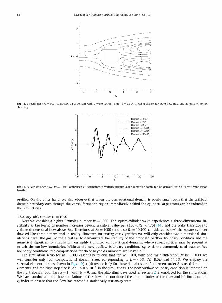
in the cylinder wake vanishes and the flow exhibits a steady state. This is demonstrated by Fig. 13, which uses streamlinesto show the steady-state flow with two re-circulation bubbles in the cylinder wake. This is obtained on a domain with wakeregion length L = 2.5D .

The observed disappearance of vortex shedding on extremely small domains in current simulations is consistent withthe stability theory and the mechanism for the onset of vortex formation in bluff-body wakes [25,18]. The vortex formationregion is the region of immediate cylinder wake where vortex shedding is initiated. This region is one of global absoluteinstability [18,47,51], which is responsible for the formation of vortex street in the cylinder wake. The end of the vortexformation region marks the initial position of fully shed vortex and the location at which the vortex strength is a maximum[18]. The length of vortex formation region, i.e. its extent in the streamwise direction, is about 2.8D behind the cylinderat Re = 100 based on experimental measurements [16,18]. Our numerical experiments and observations suggest that, whenthe wake region length of the computational domain is overly small (smaller than the vortex formation region length), ittends to disrupt the vortex formation in the cylinder wake. As a result, vortex shedding will not appear in the simulationson such a computational domain.

Next we provide some quantitative comparisons of simulation results from different computational domains. In Fig. 14we compare profiles of the instantaneous vorticity at t = 40 along the centerline (i.e. y = 0) obtained with different do-main sizes. One can observe that the vorticity oscillates around zero in the cylinder wake, and its amplitude decreaseswith increasing downstream distance from the cylinder. Compared with the vorticity profile from the largest computationaldomain (L = 24.5D), the profile from the domain L = 4.5D exhibits some pronounced difference, which manifests primarily

S. Dong et al. / Journal of Computational Physics 261 (2014) 83–105 97

Fig. 12. (Color online.) Comparison of instantaneous vorticity contours computed on domains with different wake region lengths: (a) 4.5D , (b) 7D , (c) 9.5D ,(d) 14.5D , (e) 19.5D , (f) 24.5D . Identical contour levels are shown in different plots.

as a shift in the phase but also in terms of vorticity amplitude. A very slight shift in phase can also be observed in theprofile for the domain L = 7D compared to that for L = 24.5D . On the other hand, the profiles for domains L = 9.5D , 14.5Dand 19.5D essentially overlap with that for domain L = 24.5D , and only slight difference can be discerned near the outflowboundary.

In Fig. 15 we show profiles of the instantaneous streamwise velocity at t = 40 at several downstream locations in thecylinder wake. In Figs. 15(a)–(e) we respectively compare velocity profiles obtained on domains L = 4.5D , 7D , 9.5D , 14.5Dand 19.5D against the profile for the domain L = 24.5D . We observe that the velocity profiles for domains L = 9.5D , 14.5Dand 19.5D overlap with those for L = 24.5D at essentially all downstream locations considered here. The velocity profilefor the domain L = 4.5D shows some pronounced discrepancy compared to that from domain L = 24.5D . For the domainL = 7D , some differences can be noted in the velocity profiles (especially at location x/D = 6.0) compared to those ofL = 24.5D , but they are quite slight.

The above results at Re = 100 indicate that the proposed outflow boundary condition and associated numerical algorithmcan produce accurate results on different computational domains, in terms of both global flow parameters and detailed flow

98 S. Dong et al. / Journal of Computational Physics 261 (2014) 83–105

Fig. 13. Streamlines (Re = 100) computed on a domain with a wake region length L = 2.5D , showing the steady-state flow field and absence of vortexshedding.

Fig. 14. Square cylinder flow (Re = 100): Comparison of instantaneous vorticity profiles along centerline computed on domains with different wake regionlengths.

profiles. On the other hand, we also observe that when the computational domain is overly small, such that the artificialdomain boundary cuts through the vortex formation region immediately behind the cylinder, large errors can be induced inthe simulations.

3.3.2. Reynolds number Re = 1000Next we consider a higher Reynolds number Re = 1000. The square-cylinder wake experiences a three-dimensional in-

stability as the Reynolds number increases beyond a critical value Rec (150 < Rec < 175) [44], and the wake transitions toa three-dimensional flow above Rec . Therefore, at Re = 1000 (and also Re = 10,000 considered below) the square-cylinderflow will be three-dimensional in reality. However, for testing our algorithm we will only consider two-dimensional sim-ulations here. The goal of these tests is to demonstrate the stability of the proposed outflow boundary condition and thenumerical algorithm for simulations on highly truncated computational domains, where strong vortices may be present ator exit the outflow boundaries. Without the new outflow boundary condition, e.g. with the commonly-used traction-freeboundary conditions, the computations for these Reynolds numbers are unstable.

The simulation setup for Re = 1000 essentially follows that for Re = 100, with one main difference. At Re = 1000, wewill consider only four computational domain sizes, corresponding to L = 4.5D , 7D , 9.5D and 14.5D . We employ thespectral element meshes shown in Figs. 10(a)–(d) respectively for these domain sizes. An element order 8 is used for all theelements, and the time step size is �t = 5.0 × 10−4 in the simulations. The new outflow boundary condition is imposed onthe right domain boundary x = Lx with fb = 0, and the algorithm developed in Section 2 is employed for the simulations.We have conducted long-time simulations of the flow, and monitored the time histories of the drag and lift forces on thecylinder to ensure that the flow has reached a statistically stationary state.

S. Dong et al. / Journal of Computational Physics 261 (2014) 83–105 99

Fig. 15. Square cylinder flow (Re = 100): Comparison of instantaneous streamwise velocity profiles at several downstream locations computed on domainswith different wake region lengths.

Fig. 16 shows the instantaneous velocity fields of the cylinder wake at Re = 1000 obtained with different domain sizes.The vortex shedding has apparently become quite irregular, unlike the lower Reynolds number Re = 100 (Fig. 12). The wakeregion lengths of all the computational domains considered here are quite limited with respect to this Reynolds number,in the sense that none of them are long enough for the vortices generated at the cylinder to dissipate before reaching theoutflow boundary. This is clearly demonstrated by the vortices at or near the outflow boundary in Figs. 16(b) and 16(d).These results show that the outflow boundary condition and the numerical algorithm developed in Section 2 are effectivefor flow situations where strong vortices may be present at or exit outflow boundaries. For comparison, we have alsosimulated this problem using the commonly-used traction-free outflow boundary condition [46] and its variant no-fluxoutflow condition ( ∂u

∂n = 0 and p = 0). We observe that these computations blow up instantly when the vortices hit theoutflow boundary.

In Fig. 17 we plot time histories of the drag and lift forces on the cylinder at Re = 1000 obtained on domains with wakeregion lengths 7D and 14.5D . It is evident that the drag and lift forces fluctuate about a constant mean value or about zero,and that their fluctuations are very irregular. The long-time characteristics of the force signals indicate that the flow is ata statistically stationary state. The results demonstrate that the simulations with the new outflow boundary condition andalgorithm developed in Section 2 are stable with different domain sizes over a long time. The drag and lift force signalsobtained on different domains appear qualitatively similar.

100 S. Dong et al. / Journal of Computational Physics 261 (2014) 83–105

Fig. 16. Instantaneous velocity fields of square cylinder flow at Re = 1000, computed using domains with wake region lengths: (a) 4.5D , (b) 7D , (c) 9.5D ,and (d) 14.5D . Velocity vectors are plotted on every sixth quadrature point in each direction within each element.

Fig. 17. Square cylinder flow (Re = 1000): time histories of the drag (left column) and lift (right column) forces on the cylinder computed on domains withdifferent wake region lengths, 7D (a, b), and 14.5D (c, d).

To provide a quantitative comparison of results from different domains, in Table 4 we list global flow parameters com-

puted from the time histories of the forces on the cylinder. These include the mean drag coefficient Cd = 2Fx

ρU 20

, r.m.s. drag

coefficient C ′d = 2F ′

x

ρU 20

(F ′x denotes the r.m.s. drag force), r.m.s. lift coefficient CL = 2F ′

y

ρU 20

(F ′y denotes the r.m.s. lift force), and

the Strouhal number St = f DU0

( f denotes the frequency of vortex shedding). The vortex shedding frequency is computedbased on the time history of the lift force. For comparison, we have also included the mean drag coefficient value fromthe experiment [48]. First, we observe that the global flow parameter values computed on domains with L = 7D , 9.5Dand 14.5D are very close to one another. If we use the parameter values from the domain L = 14.5D as reference, thenthe largest difference in the mean and r.m.s. drag coefficients is less than 2%, and the largest difference in the r.m.s. lift

S. Dong et al. / Journal of Computational Physics 261 (2014) 83–105 101

Table 4Global flow parameters for square cylinder flow at Re = 1000, obtained on domains with different wake region lengths. mean drag coefficient, Cd = 2Fx

ρU 20

;

r.m.s. drag coefficient, C ′d = 2F ′

x

ρU 20

; r.m.s. lift coefficient, CL = 2F ′y

ρU 20

; Strouhal number St = f D/U0. Fx is the time-averaged mean drag force. F ′x and F ′

y

respectively denote the r.m.s. drag force and r.m.s. lift force. f denotes the vortex shedding frequency determined from the lift force history.

Source/wake region lengths Cd C ′d CL St

Present study, L = 4.5D 2.501 0.809 1.640 0.0878Present study, L = 7D 2.654 0.879 1.630 0.0930Present study, L = 9.5D 2.579 0.871 1.678 0.0970Present study, L = 14.5D 2.628 0.884 1.694 0.0971Shimizu & Tanida (experiment) [48] 2.3 – – –

Fig. 18. Spectral element meshes with (a) 736 and (b) 992 quadrilateral elements for the square cylinder flow at Re = 10,000.

coefficient and in the Strouhal number is about 4%. On the other hand, the parameter values from the smallest domainL = 4.5D exhibit a slightly larger difference compared to those from the domain L = 14.5D (4.8% in mean drag coefficient,8.5% in r.m.s. drag coefficient, 3.2% in r.m.s. lift coefficient, and 9.6% in Strouhal number). Compared to the experimentalvalue for the mean drag coefficient, the values obtained from the current two-dimensional simulations are comparable, butconsistently a little larger. The discrepancy is likely due to the three-dimensional effects at such a Reynolds number.

3.3.3. Reynolds number Re = 10,000The last test case is the square cylinder flow at an even higher Reynolds number Re = 10,000. For this test we consider

a smaller dimension, L y/D = 4, in the y direction. The periodic boundary condition is imposed at y = L y and y = −L y .Because of the significant blockage ratio, the setup corresponds to the flow past an array of square cylinders which arealigned in the y direction. We will consider two computational domains with the right boundary at Lx = 6D and Lx = 14D ,respectively, giving rise to wake region lengths L = 5.5D and L = 13.5D . Fig. 18 shows the spectral-element meshes forthese two domains, with 736 and 992 quadrilateral elements respectively. We use an element order 14 for all the elementsin the mesh, and the time step size in the simulations is �t = 5.0 × 10−5 for this Reynolds number.

For the initial condition at Re = 10,000 the velocity field from a lower Reynolds number has been used. The flow issimulated for a long time, and the forces on the cylinder are monitored to ensure that the flow has evolved to a statisticallystationary state.

In Fig. 1 we show a snapshot of the instantaneous velocity field, together with the pressure distribution, at Re = 10,000obtained on the domain with wake region length L = 5.5D , and in Fig. 19 we show a snapshot of the instantaneous velocityand pressure fields on the larger domain L = 13.5D . One can observe a large number of vortices in the wake and alsoon the top and bottom surfaces of the cylinder. The spatial scales of the vortices are considerably smaller than thoseof lower Reynolds numbers (see e.g. Fig. 16 for Re = 1000). Vortices can be clearly observed at the outflow boundaries(Figs. 1 and 19). The new outflow boundary condition and the numerical algorithm are stable for these flow situations. Forcomparison, the usual traction-free outflow boundary condition and its variant no-flux boundary condition have also beentested at Re = 10,000 for this problem, and both are unstable.

Fig. 20 shows time histories of the drag and lift forces acting on the cylinder obtained with different domain sizes.Fig. 20(a) corresponds to the computational domain with wake region length L = 5.5D , and Fig. 20(b) corresponds to the

102 S. Dong et al. / Journal of Computational Physics 261 (2014) 83–105

Fig. 19. (Color online.) Instantaneous velocity field, and pressure contours (in color), of the square cylinder flow at Re = 10,000 computed on a domain withwake region length L = 13.5D . Velocity vectors are plotted on every fourth quadrature point in each direction within each element.

Fig. 20. Square cylinder flow at Re = 10,000: Time histories of the drag and lift forces acting on the cylinder obtained on computational domains with wakeregion lengths (a) L = 5.5D and (b) L = 13.5D .

Table 5Global force parameters obtained with two different domain sizes for the square cylinder flow at Re = 10,000.Cd , mean drag coefficient; C ′

d , r.m.s. drag coefficient; CL , r.m.s. lift coefficient.

Wake region lengths Cd C ′d CL

L = 5.5D 1.479 0.333 0.804L = 13.5D 1.491 0.366 0.825

wake region length L = 13.5D . One can observe that the force signals at this Reynolds number are very chaotic and thatboth forces exhibit strong high-frequency fluctuations. These time histories further demonstrate the stability of the newoutflow boundary condition and the numerical algorithm developed in Section 2 for long-time simulations at Re = 10,000,where strong vortices are present at and exiting the outflow boundary. The time histories obtained with the smaller domainL = 5.5D appear qualitatively similar to those from the larger domain L = 13.5D .

A quantitative comparison of the results obtained with the two different domain sizes are provided in Table 5 with theglobal flow parameters at Re = 10,000. We have listed the mean drag coefficient Cd , r.m.s. drag coefficient C ′ and r.m.s.

d

S. Dong et al. / Journal of Computational Physics 261 (2014) 83–105 103

lift coefficient CL obtained with the two domain sizes. The Strouhal number is not provided in the table, because a reliabledetermination of the frequency requires a very long time history and this is associated with a large computational cost atRe = 10,000. The mean drag coefficient and the r.m.s. lift coefficient obtained on the smaller computational domain L = 5.5Dagree very well with those from the larger domain L = 13.5D , with a difference < 1% for the mean drag coefficient and2.5% for the r.m.s. lift coefficient. The r.m.s. drag coefficient obtained from the smaller domain is close to, but somewhatsmaller than, that from the larger domain, with a difference of about 9%.

4. Concluding remarks

In this paper we have presented a new outflow boundary condition, and an algorithm for dealing with this boundarycondition, for incompressible flow simulations on highly-truncated unbounded domains. This outflow boundary conditionis designed in such a way that the kinetic-energy influx into the domain through the outflow boundary will not causeun-controlled growth in the energy of the domain. The main idea can be summarized as follows: if anywhere on the outflowboundary there is an energy influx into the domain then the stress on the outflow boundary shall locally balance the effective stressinduced by the energy influx, otherwise the stress shall locally vanish.

Our numerical algorithm for this outflow boundary condition is developed on top of a rotational velocity-correction typestrategy for the incompressible Navier–Stokes equations. At the pressure step, we impose a discrete Dirichlet condition forthe pressure on the outflow boundaries, which is derived from the proposed outflow boundary condition. At the velocitystep, we impose a discrete Neumann condition for the velocity on the outflow boundaries. The discrete velocity Neumanncondition stems essentially from the proposed outflow boundary condition, but contains extra construction to prevent anumerical locking on the outflow boundary for time-dependent problems. While it is implemented with a spectral-elementspatial discretization in the current paper, the proposed algorithm is very general and can be implemented with other typesof spatial discretizations such as finite elements or finite differences.

The outflow boundary condition and the numerical algorithm developed herein are very robust and accurate. Extensivenumerical experiments demonstrate that this outflow boundary condition and numerical algorithm produce stable simu-lations, even on computational domains that are severely truncated, where strong vortices may be present at or exit theoutflow boundaries. A range of Reynolds numbers has been tested, from low to moderate to high values (up to Re = 10,000in numerical simulations). In contrast, the commonly-used traction-free outflow boundary condition (and its variant no-fluxoutflow condition) are unstable in these tests, and blow up instantly when the vortices hit the outflow boundaries.

Systematic tests have been performed, by varying the length of the outflow region, to investigate the effects of differentdomain sizes on the simulation results. These tests indicate that as the domain size decreases the change in the simulationresults is very little, in terms of both global flow parameters and detailed flow profiles, as long as the computational domainis not extremely small. On the other hand, we would like to point out that the outflow boundary condition is no substitutefor the flow physics, and that an extremely small computational domain can disrupt the flow mechanisms and affect theflow physics. For example, in the flow past a cylinder, when the wake region length is smaller than the length of vortexformation region (or region of absolute instability), which is typically about two to three times the cylinder dimension andis Reynolds-number dependent, our tests show that it can disrupt the formation of vortices in the cylinder wake. As a result,a simulation on such an extremely confined domain would result in a steady-state flow at a Reynolds number that is knownto lead to vortex shedding and a vortex street in the wake under normal conditions.

The outflow boundary condition and the numerical algorithm developed in the current paper have the potential tosignificantly expedite flow simulations involving wakes, jets, and other situations where outflow or open boundaries areinvolved, especially for high Reynolds numbers. Owing to the numerical instability caused by vortices at outflow boundaries,current flow simulations usually require very large computational domains to achieve stability, in order for the vortices tobe sufficiently dissipated before reaching the outflow boundaries. The proposed outflow boundary condition and numericalalgorithm provide an effective and robust method for stable simulations on even severely truncated computational domainswhere strong vortices may be present at the outflow boundaries. With the current method, the choice of the computationaldomain size is only restricted by the consideration of physical accuracy, not by numerical stability associated with theoutflow boundary. Because all the grid resolution only need to be placed in a small computational domain, the currentmethod can potentially enable simulations at Reynolds numbers significantly higher than the state of the art.

Finally, we would like to caution that the outflow boundary condition and the algorithm in the current paper are devel-oped based on the incompressible Navier–Stokes equations. If the form of the governing equations changes, e.g. with thearbitrary Lagrangian–Eulerian (ALE) formulations or when multiple fluid phases are involved, a consistent outflow boundarycondition will require corresponding changes. Such issues will be considered in future studies.

Acknowledgement

The authors gratefully acknowledge the support from ESRDC, ONR and NSF. Computer time was provided by XSEDEthrough an XRAC grant.

104 S. Dong et al. / Journal of Computational Physics 261 (2014) 83–105

References

[1] M. Behr, J. Liou, R. Shih, T.E. Tezduyar, Vorticity-streamfunction formulation of unsteady incompressible flow past a cylinder sensitivity of the computedflow field to the location of the outflow boundary, Int. J. Numer. Methods Fluids 12 (1991) 323–342.

[2] C.-H. Bruneau, P. Fabrie, Effective downstream boundary conditions for incompressible Navier–Stokes equations, Int. J. Numer. Methods Fluids 19 (1994)693–705.

[3] T. Colonius, Modeling artificial boundary conditions for compressible flow, Annu. Rev. Fluid Mech. 36 (2004) 315–345.[4] R.W. Davis, E.F. Moore, A numerical study of vortex shedding from rectangles, J. Fluid Mech. 116 (1982) 475.[5] S. Dong, BDF-like methods for nonlinear dynamic analysis, J. Comput. Phys. 229 (2010) 3019–3045.[6] S. Dong, G.E. Karniadakis, DNS of flow past stationary and oscillating cylinder at Re = 10,000, J. Fluids Struct. 20 (2005) 14–23.[7] S. Dong, G.E. Karniadakis, A. Ekmekci, D. Rockwell, A combined direct numerical simulation-particle image velocimetry study of the turbulent near

wake, J. Fluid Mech. 569 (2006) 185–207.[8] S. Dong, J. Shen, An unconditionally stable rotational velocity-correction scheme for incompressible flows, J. Comput. Phys. 229 (2010) 7013–7029.[9] S. Dong, J. Shen, A time-stepping scheme involving constant coefficient matrices for phase field simulations of two-phase incompressible flows with

large density ratios, J. Comput. Phys. 231 (2012) 5788–5804.[10] M.S. Engelman, M.-A. Jamnia, Transient flow past a circular cylinder: A benchmark solution, Int. J. Numer. Methods Fluids 11 (1990) 985–1000.[11] M.Y. Forestier, R. Pasquetti, R. Peuret, C. Sabbah, Spatial development of wakes using a spectral multi-domain method, Appl. Numer. Math. 33 (2000)

207–216.[12] L. Formaggia, J.-F. Gerbeau, F. Nobile, A. Quarteroni, Numerical treatment of defective boundary conditions for the Navier–Stokes equations, SIAM J.

Numer. Anal. 40 (2002) 376–401.[13] R. Franke, B. Schonung, Numerical calculation of laminar vortex shedding flow past cylinders, J. Wind Eng. Ind. Aerodyn. 35 (1990) 237.[14] D.K. Gartling, A test problem for outflow boundary conditions – flow over a backward-facing step, Int. J. Numer. Methods Fluids 11 (1990) 953–967.[15] D. Givoli, High-order local non-reflecting boundary conditions: a review, Wave Motion 39 (2004) 319–326.[16] R.B. Green, J.H. Gerrard, Vorticity measurements in the near wake of a circular cylinder at low Reynolds numbers, J. Fluid Mech. 246 (1993) 675–691.[17] P.M. Gresho, Incompressible fluid dynamics: some fundamental formulation issues, Annu. Rev. Fluid Mech. 23 (1991) 413–453.[18] O.M. Griffin, A note on bluff body vortex formation, J. Fluid Mech. 284 (1995) 217–224.[19] D.F. Griffiths, The ‘no boundary condition’ outflow boundary condition, Int. J. Numer. Methods Fluids 24 (1997) 393–411.[20] L. Grinberg, G.E. Karniadakis, Outflow boundary conditions for arterial networks with multiple outlets, Ann. Biomed. Eng. 36 (2008) 1496–1514.[21] J.L. Guermond, P. Minev, J. Shen, Error analysis of pressure-correction schemes for the time-dependent Stokes equations with open boundary conditions,

SIAM J. Numer. Anal. 43 (2005) 239–258.[22] J.L. Guermond, J. Shen, Velocity-correction projection methods for incompressible flows, SIAM J. Numer. Anal. 41 (2003) 112–134.[23] N. Hasan, S.F. Anwer, S. Sanghi, On the outflow boundary condition for external incompressible flows: a new approach, J. Comput. Phys. 206 (2005)

661–683.[24] J.G. Heywood, R. Rannacher, S. Turek, Artificial boundaries and flux and pressure: conditions for the incompressible Navier–Stokes equations, Int. J.

Numer. Methods Fluids 22 (1996) 325–352.[25] P. Huerre, P.A. Monkewitz, Local and global instabilities in spatially developing flows, Annu. Rev. Fluid Mech. 22 (1990) 473.[26] G. Jin, M. Braza, A nonreflecting outlet boundary condition for incompressible unsteady Navier–Stokes calculations, J. Comput. Phys. 107 (1993)

239–253.[27] B.C.V. Johansson, Boundary conditions for open boundaries for the incompressible Navier–Stokes equation, J. Comput. Phys. 105 (1993) 233–251.[28] G.E. Karniadakis, S.J. Sherwin, Spectral/hp Element Methods for Computational Fluid Dynamics, 2nd edn., Oxford University Press, 2005.[29] K.M. Kelkar, S. Patankar, Numerical prediction of vortex shedding behind a square cylinder, Int. J. Numer. Methods Fluids (2013).[30] J. Keskar, D.A. Lyn, Computations of a laminar backward-facing step flow at Re = 800 with a spectral domain decomposition method, Int. J. Numer.

Methods Fluids 29 (1999) 411–427.[31] H.J. Kim, C.A. Figueroa, T.J.R. Hughes, K.E. Jansen, C.A. Taylor, Segmented langrangian method for constraining the shape of velocity profiles at outlet

boundaries for three-dimensional finite element simulations of blood flow, Comput. Methods Appl. Mech. Eng. 198 (2009) 3551–3566.[32] L.I.G. Kovasznay, Laminar flow behind a two-dimensional grid, Proc. Camb. Philol. Soc. 44 (1948) 58.[33] J.M. Leone, Open boundary condition symposium benchmark solution: stratified flow over a backward-facing step, Int. J. Numer. Methods Fluids 11

(1990) 969–984.[34] J. Liu, Open and traction boundary conditions for the incompressible Navier–Stokes equations, J. Comput. Phys. 228 (2009) 7250–7267.[35] J. Nordstrom, K. Mattsson, C. Swanson, Boundary conditions for a divergence free velocity-free formulation of the Navier–Stokes equations, J. Comput.

Phys. (2007) 874–890.[36] J. Nordstrom, M. Svard, Well-posed boundary conditions for the Navier–Stokes equations, SIAM J. Numer. Anal. 43 (2005) 1231–1255.[37] A. Okajima, Strouhal numbers of rectangular cylinders, J. Fluid Mech. 123 (1982) 379–398.[38] M.A. Olshanskii, V.M. Staroverov, On simulation of outflow boundary conditions in finite difference calculations for incompressible fluid, Int. J. Numer.

Methods Fluids 33 (2000) 499–534.[39] I. Orlanski, A simple boundary condition for unbounded hyperbolic flows, J. Comput. Phys. 21 (1976) 251–269.[40] T.C. Papanastasiou, N. Malamataris, K. Ellwood, A new outflow boundary condition, Int. J. Numer. Methods Fluids 14 (1992) 587–608.[41] A. Poux, S. Glockner, E. Ahusborde, M. Azaiez, Open boundary conditions for the velocity-correction scheme of the Navier–Stokes equations, Comput.

Fluids 70 (2012) 29–43.[42] A. Poux, S. Glockner, M. Azaiez, Improvements on open and traction boundary conditions for Navier–Stokes time-splitting methods, J. Comput. Phys.

230 (2011) 4011–4027.[43] M. Renardy, Imposing ‘no’ boundary condition at outflow: why does it work?, Int. J. Numer. Methods Fluids 24 (1997) 413–417.[44] J. Robichaux, S. Balachandar, S.P. Vanka, Three-dimensional Floquet instability of the wake of square cylinder, Phys. Fluids 11 (1999) 560–578.[45] M.R. Ruith, P. Chen, E. Meiburg, Development of boundary conditions for direct numerical simulations of three-dimensional vortex breakdown phe-

nomena in semi-infinite domains, Comput. Fluids 33 (2004) 1225–1250.[46] R.L. Sani, P.M. Gresho, Resume and remarks on the open boundary condition minisymposium, Int. J. Numer. Methods Fluids 18 (1994) 983–1008.[47] M. Schumm, E. Berger, P.A. Monkewitz, Self-excited oscillations in the wake of two-dimensional bluff bodies and their control, J. Fluid Mech. 271

(1994) 17–53.[48] Y. Shimizu, Y. Tanida, Fluid forces acting on cylinders of rectangular cross-section, Trans. Jpn. Soc. Mech. Eng. B (2013) 44.[49] A. Sohankar, C. Norberg, L. Davidson, Low Reynolds number flow around a square cylinder at incidence: study of blockage, onset of vortex shedding,

and open boundary conditions, Int. J. Numer. Methods Fluids 26 (1998) 39.[50] S. Taylor, J. Rance, J.O. Medwell, A note on the imposition of traction boundary conditions when using the FEM for solving incompressible flow

problems, Commun. Appl. Numer. Methods 1 (1985) 113–121.

S. Dong et al. / Journal of Computational Physics 261 (2014) 83–105 105

[51] G.S. Triantafyllou, M.S. Triantafyllou, C. Chryssostomidis, On the formation of vortex streets behind stationary cylinders, J. Fluid Mech. 170 (1986)461–477.

[52] S.V. Tsynkov, Numerical solution of problems on unbounded domains: A review, Appl. Numer. Math. 27 (1998) 465–532.[53] X. Zheng, S. Dong, An eigen-based high-order expansion basis for structured spectral elements, J. Comput. Phys. 230 (2011) 8573–8602.