Embed Size (px)
Citation preview

University of Tennessee, Knoxville University of Tennessee, Knoxville
TRACE: Tennessee Research and Creative TRACE: Tennessee Research and Creative
Exchange Exchange
Masters Theses Graduate School
12-2019
A Robust Hierarchical Dispatch Scheme for Active Distribution A Robust Hierarchical Dispatch Scheme for Active Distribution
Networks Considering Home Thermal Flexibility Networks Considering Home Thermal Flexibility
Cody Rooks University of Tennessee, [email protected]
Follow this and additional works at: https://trace.tennessee.edu/utk_gradthes
Recommended Citation Recommended Citation Rooks, Cody, "A Robust Hierarchical Dispatch Scheme for Active Distribution Networks Considering Home Thermal Flexibility. " Master's Thesis, University of Tennessee, 2019. https://trace.tennessee.edu/utk_gradthes/5577
This Thesis is brought to you for free and open access by the Graduate School at TRACE: Tennessee Research and Creative Exchange. It has been accepted for inclusion in Masters Theses by an authorized administrator of TRACE: Tennessee Research and Creative Exchange. For more information, please contact [email protected].

To the Graduate Council:
I am submitting herewith a thesis written by Cody Rooks entitled "A Robust Hierarchical
Dispatch Scheme for Active Distribution Networks Considering Home Thermal Flexibility." I have
examined the final electronic copy of this thesis for form and content and recommend that it be
accepted in partial fulfillment of the requirements for the degree of Master of Science, with a
major in Electrical Engineering.
Fangxing Li PhD, Major Professor
We have read this thesis and recommend its acceptance:
Leon Tolbert PhD, Mohammed Olama PhD
Accepted for the Council:
Dixie L. Thompson
Vice Provost and Dean of the Graduate School
(Original signatures are on file with official student records.)
A Robust Hierarchical Dispatch Scheme for Active Distribution Networks Considering Home Thermal Flexibility
A Thesis Presented for the
Master of Science Degree
The University of Tennessee, Knoxville
Cody Davis Rooks December 2019

ii
Copyright © 2019 by Cody Davis Rooks All rights reserved.

iii
DEDICATION I dedicate this thesis to my family and friends.

iv
ACKNOWLEDGEMENTS I first and foremost would like to thank my advisor and mentor, Dr.
Fangxing “Fran” Li, for his mentorship, instruction, scholarship and general
facilitation of my graduate academic ambitions. I hope that he remains a lifelong
mentor and friend.
I would also like to extend a tremendous thanks to my thesis committee
members, Dr. Leon Tolbert and Dr. Mohammed Olama, for both their
participation in my thesis proceedings as well as the instruction and direction I
received through coursework and supervision.
I would additionally like to thank my mentors and colleagues at Oak Ridge
National Laboratory (ORNL) for their guidance and support of my work, including
Dr. Jin Dong, Dr. Teja Kuruganti, Dr. Christopher Winstead, Dr. Michael Starke,
Dr. Yaosuo “Sonny” Xue and Dr. Alexander Melin.
I am grateful for the guidance and assistance I received from my research
group colleagues over the course of my graduate program, including Xiao Kou,
Dr. Hantao Cui, Mariana Kamel, Dr. Qingxin Shi, Qiwei Zhang, Wei Feng and
Yan Du.
I am also grateful to the National Science Foundation (NSF) and
corresponding funding opportunities made available to me through the Center for
Ultra-Wide-Area Resilient Electric Energy Transmission Networks (CURENT).
Finally, I would like to thank my parents and greater family for their
unconditional love and support of my myriad pursuits.

v
ABSTRACT Distribution networks are changing from passive absorbers of electric
energy to active distribution networks (ADNs) capable of operating and
participating in electricity markets. In the context of residential microgrids, which
are a type of ADN, aggregated home heating, ventilation and air-conditioning
(HVAC) loads present a key opportunity to drive operational and economic
objectives, facilitate high renewable energy penetration, and enhance both
system resiliency and flexibility. A robust, hierarchical dispatch scheme is
developed and presented in this thesis, which connects an upper level, multi-
phase distribution optimal power flow (DOPF) to a lower level model predictive
control (MPC)-based HVAC fleet controller. The approach is tested and verified
on a modified IEEE 13 bus system in an intraday market application. The results
demonstrate that the proposed hierarchical dispatch scheme is able to drive both
economic and operational objectives for the ADN operator.
vi
TABLE OF CONTENTS
INTRODUCTION .................................................................................................. 1 Background ....................................................................................................... 2 Relevant Literature ............................................................................................ 5 Contributions and Organization ......................................................................... 7
CHAPTER I DISTRIBUTION OPTIMAL POWER FLOW ...................................... 8
Overview ........................................................................................................... 9 Distribution System Modelling ......................................................................... 11
Review of Approaches ................................................................................. 11 Multi-phase LinDistFlow Approach .............................................................. 13
Robust Optimization ........................................................................................ 18
Review of Approaches ................................................................................. 18
Interval Optimization Approach .................................................................... 19
CHAPTER II HVAC FLEET CONTROL .............................................................. 24
Home Thermal Modelling ................................................................................ 25 Model Predictive Control Approach ................................................................. 27
Classical Approach ...................................................................................... 27
Modified Approach ....................................................................................... 28 CHAPTER III APPLICATIONS AND DISCUSSION ............................................ 30
Problem Formulation ....................................................................................... 31 Overview ...................................................................................................... 31 Upper Level ................................................................................................. 31
Lower Level ................................................................................................. 35 Solution Approach ........................................................................................... 37
Case Study ...................................................................................................... 39 Description of System .................................................................................. 39
Simulation Environment ............................................................................... 42 Application 1. Load Shaping, Peak Reduction ............................................. 44 Application 2. Load Shaping, High Renewable Injection .............................. 49
Application 3. Black Start Enhancement ...................................................... 54 CONCLUSIONS.................................................................................................. 60
REFERENCES ................................................................................................... 63 APPENDIX .......................................................................................................... 71
Appendix A. System Identification Approach ................................................... 72
Appendix B. IEEE 13-bus System Data .......................................................... 73 VITA .................................................................................................................... 74

vii
LIST OF TABLES
Table 1. Fleet controller design parameters. ....................................................... 35 Table 2. Flexible homes at each bus and phase. ................................................ 40 Table 3. Total cost comparison of base case and flexible case. ......................... 46 Table 4. Solar injection as proportion of total energy. ......................................... 50 Table 5. Solar injection as proportion of peak capacity. ...................................... 50
Table 6. Comparison of reliability metrics. .......................................................... 59 Table 7. System base data. ................................................................................ 73 Table 8. Branch data. .......................................................................................... 73
viii
LIST OF FIGURES
Figure 1. Proposed transactive energy environment [7]. ....................................... 3 Figure 2. Simple single-phase radial distribution diagram. .................................. 14 Figure 3. Simple three-phase radial distribution diagram. ................................... 15 Figure 4. Multi-phase LinDistFlow error vs. voltage imbalance (top – using self
impedance, bottom - pos. seq. impedance) ................................................. 16
Figure 5. Indoor air temperature. ........................................................................ 26 Figure 6. Example interval parameter. ................................................................ 34 Figure 7. Algorithmic overview. ........................................................................... 37 Figure 8. Temporal overview of control hierarchy. .............................................. 38 Figure 9. IEEE standard 13-bus system (left) and modified multi-phase version
(right). .......................................................................................................... 39
Figure 10. Typical summer day LMP [52]. .......................................................... 40
Figure 11. Temperature band distributions by phase and bus. ........................... 41
Figure 12. Outdoor temperature for a typical late summer day in Southeastern U.S. .............................................................................................................. 42
Figure 13. Simulation overview for implementation of case studies. ................... 43
Figure 14. App. 1 - Inflexible total power injection by phase. .............................. 44 Figure 15. App. 1 - Total power importation (blue – base case, red – flexible
case). ........................................................................................................... 45 Figure 16. App. 1 - Reference power tracking and error by phase and bus. ....... 47 Figure 17. App. 1 - Average temperatures by phase and bus (left - base case,
right – flexible case). .................................................................................... 47 Figure 18. App. 1 – Maximum power imbalance (upper - base case, lower –
flexible case). ............................................................................................... 48 Figure 19. App. 2 - Inflexible total power injection by phase. .............................. 49
Figure 20. App. 2 - Total power importation (blue – base case, red – flexible case). ........................................................................................................... 51
Figure 21. App. 2 – Reference power tracking and error by phase and bus. ...... 52
Figure 22. App. 2 –Average temperatures by phase and bus (left – base case, right – flexible case). .................................................................................... 53
Figure 23. App. 2 – Maximum power imbalance (upper - base case, lower – flexible case). ............................................................................................... 54
Figure 24. App. 3 - Total power importation by phase (upper – base case, lower – flexible case). ............................................................................................... 55
Figure 25. App. 3 - Total power importation (blue – base case, red – flexible case). ........................................................................................................... 56
Figure 26. App. 3 - Nodal voltages by phase and bus (left - base case, right – flexible case). ............................................................................................... 56
Figure 27. App. 3 - Average temperatures by phase and bus (left - base case, right – flexible case). .................................................................................... 57
Figure 28. App. 3 - Maximum power imbalance (upper - base case, lower – flexible case). ............................................................................................... 58

1
INTRODUCTION

2
Background
Several advances are occurring in the way electricity is delivered and
consumed. These changes are primarily being driven by economic and
environmental incentives to de-carbonize an otherwise unsustainable, aged and
inefficient electric grid [1]. One major shift is the transition of distribution
networks1 as passive absorbers of electrical energy to active distribution
networks (ADN) that are capable of performing a much wider variety of functions
compared to their historical operation (note that ADN is an umbrella term that
also covers microgrids). Some of these new features include automated fault
detection and restoration, optimized control of system voltages and advanced
demand response programs, among others [2].
In tandem with this transition are the trends occurring on the customer
side of the meter, which include both technology adoption and consumer
awareness. Technologically, an increasing number of consumers are purchasing
smart appliances, solar generation systems, electric vehicles (EVs) and other
energy devices [3]. Consumer awareness refers to customer demand for greater
choice in electricity market products, as well as their increasing willingness to
engage in the electricity market, so long as incentives are properly aligned [4]. In
addition, the proliferation of home energy management systems (HEMS) creates
a connected environment that makes possible an interaction between consumers
and the larger grid [5].
In order to manage this new interaction between an ADN and its customer
base (and also the bulk power system), new electricity markets are being
developed. One promising approach put forth is the transactive energy (TE)
paradigm, which seeks to drive operational objectives through the use of
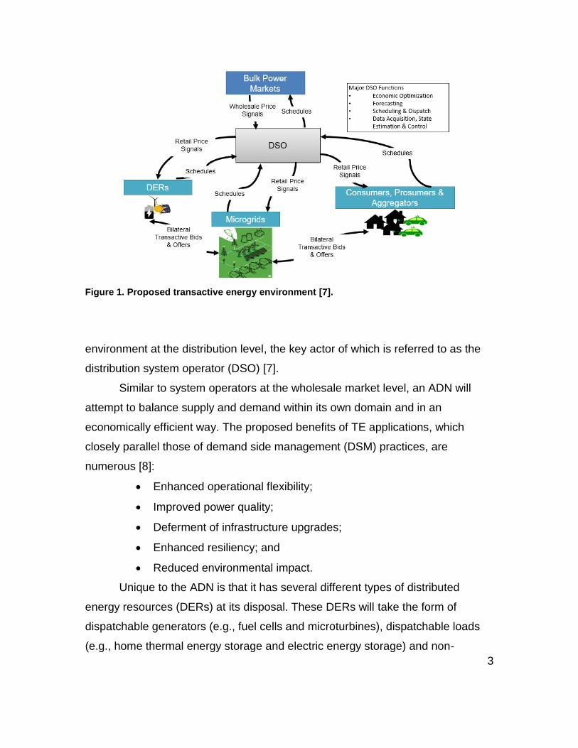
economic (price-based) incentives [6]. Figure 1 portrays a theoretical TE
1 Distribution networks refer to lower voltage power systems (typically 2.4-69 kV) that connect consumers to the bulk power system.
3
Figure 1. Proposed transactive energy environment [7].
environment at the distribution level, the key actor of which is referred to as the
distribution system operator (DSO) [7].
Similar to system operators at the wholesale market level, an ADN will
attempt to balance supply and demand within its own domain and in an
economically efficient way. The proposed benefits of TE applications, which
closely parallel those of demand side management (DSM) practices, are
numerous [8]:
• Enhanced operational flexibility;
• Improved power quality;
• Deferment of infrastructure upgrades;
• Enhanced resiliency; and
• Reduced environmental impact.
Unique to the ADN is that it has several different types of distributed
energy resources (DERs) at its disposal. These DERs will take the form of
dispatchable generators (e.g., fuel cells and microturbines), dispatchable loads
(e.g., home thermal energy storage and electric energy storage) and non-

4
dispatchable generators (e.g., solar PV and small wind turbines). Indeed, the
sheer multitude of devices capable of participating in an energy market on the
distribution network necessitates the use of aggregators, which provide an
interface between the distribution operator and its customer base. The use of
aggregators serves additional purposes: more resilient cybersecurity,
decentralized computation and communication benefits, better privacy and others
[9].
Although clearly there are several resources that could be engaged in a
TE environment, aggregated heating, ventilation and air-conditioning (HVAC)
loads present a key opportunity in terms of both pervasiveness and capacity.
According to an International Energy Agency (IEA) report, global HVAC demand,
which already accounts for around 10% of total electricity consumption, is
expected to triple by 2050 [10]. Thus, the flexibility and smart operation of this
resource has the potential to achieve more efficient, sustainable grid operations.
Aggregated HVAC systems have already been noted to have a capability to
provide grid services, including both frequency and voltage regulation [11] [12]
[13]. These services are made possible through home thermal energy storage
capacities, where a home can effectively “charge” through the running of its
HVAC system, and “discharge” through its ability to operate within a user-defined
temperature band.
This is the flexibility that is considered in this study, which presents a
hierarchical dispatch scheme connecting a residential microgrid, flexible
customer base, and the wholesale market. The next section will review some
existing literature in this area.
5
Relevant Literature
This thesis is broadly concerned with the application of an aggregated-
device-to-grid integration scheme. Such studies analyze and assess the types of
grid services that could be provided from the smart and coordinated actuation of
numerous customer-side devices, and generally how their flexibility can assist
grid operations. System flexibility has been deemed essential to successfully
integrate a high proportion of renewable energy [14].
A significant amount of prior study in this area is concerned with vehicle-
to-grid (V2G) dispatch and integration schemes, which generally attempt to
optimize the charging and discharging of a fleet of EVs to drive certain
operational or economic objectives [15]. In this light, a lot of relevant groundwork
has already been laid.
Some studies demonstrate how a fleet of EVs can shave peak demand or
minimize peak to average demand ratio [16] [17]. Peak shaving is considered a
major benefit of smart grid technologies, and is also demonstrated in this work.
The study of [18] presents a model predictive control (MPC)-based approach to
control a fleet of EVs for V2G applications. The proposed approach of this thesis
also uses an MPC-based control strategy at the lower level. Some work
investigates the impact that a fleet of EVs could have on reliability metrics [19].
Enhancement of reliability is also considered as one application of the proposed
approach. The authors in [20] demonstrate how the flexibility of a fleet of EVs can
help integrate high penetration of wind power. Similarly, this thesis considers how
a fleet of HVAC units can be modulated to integrate a high penetration of
renewable energy.
Specifically, this paper is concerned with an HVAC-based home-to-grid
(H2G) application. H2G studies are fundamentally similar to V2G studies, the
primary difference being that the HVAC fleet flexibility resource has a different
dynamic model. While an EV fleet can theoretically provide power to the grid, an
HVAC fleet provides grid services via the temporal shift of its power
consumption.

6
In general, H2G studies attempt to connect a distribution optimal power
flow (DOPF) procedure, described in the following chapter, to an aggregator,
which controls participating devices. The aggregator in this case is a home
HVAC fleet controller. The primary differences around many H2G applications
revolve around modelling assumptions and approaches of the ADN, as well as
the control function of the aggregator.
Some studies present MPC-based control approaches to optimize the
behavior of a number of home devices in terms of economic objectives [21] [22].
Yet, these do not consider the physical model and constraints of the distribution
network. The study in [23] presents a buildings-to-grid integration framework,
which uses an MPC-based control approach to coordinate building fleet
consumption with power system operations. Although the authors present
promising results, only transmission level operations are considered.
In [24], a bi-level optimization methodology is applied to coordinate the
operation of a fleet of buildings with a distribution network so that operational
constraints are satisfied. This work relies on a three-phase iterative DOPF
approach that may not scale well. The work of [25] also develops a bi-level
buildings-to-grid integration scheme; however, this study does not consider the
operational constraints of the distribution network.
The authors in [26] use an MPC approach to control an aggregation of
devices using price signals. This work also couples an aggregator with a
distribution grid, but employs a full AC power flow procedure, which may
encounter computational difficulties. The approach in [27] also solves an AC
power flow, but assumes balanced conditions, which may not always be practical
or suitable to distribution networks.

7
Contributions and Organization
The main contribution of this thesis is a novel, practical H2G integration
scheme, which couples a robust, linear multi-phase DOPF with an MPC-based
HVAC fleet controller. The approach is tested in a number of scenarios and
applications on a modified IEEE 13-bus test system in an intraday market
context. The structure of this paper is organized as follows:
• Chapter 1 presents the primary functionality of the upper level network
optimizer – namely, the formulation and solution strategy of a robust,
DOPF procedure for an unbalanced, three-phase distribution network.
• Chapter 2 presents the lower level HVAC fleet controller, including
subsections on home thermal modelling as well as the MPC-based control
approach.
• Chapter 3 presents the entire problem formulation, its solution approach
and finally simulation results and discussion.
• The last chapter provides a conclusion, including some notes on future
work.

8
CHAPTER I DISTRIBUTION OPTIMAL POWER FLOW
9
Overview
Optimal power flow (OPF) is a classical power systems analysis problem.
Its history can be traced back to the deregulation of the bulk power system and
establishment of the wholesale market, where power generation companies were
granted equal and open access to the transmission network [28].
OPF is essentially the mathematical coupling of the economic dispatch
(ED) problem with the power flow problem [29]. In other words, a lowest cost
dispatch solution is computed subject to the constraints of the network. Network
constraints must be considered to ensure stability and health of the system so
that decisions made in the optimization procedure do not result in operational
violations.
In standard practice, OPF is the formulation of an optimization problem.
Thus, the core of OPF is the underlying system model. It is this model that
determines the type of optimization problem, as well as its solution approach. In
this context, the historical development of OPF is strongly associated with the
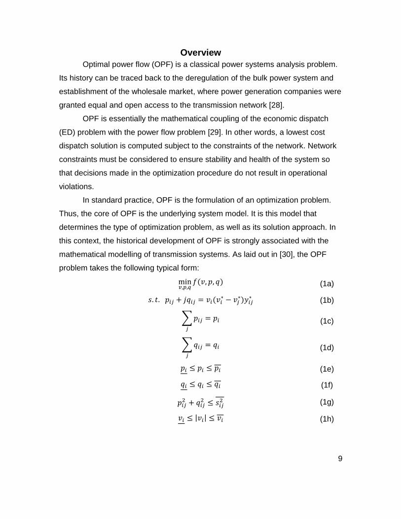
mathematical modelling of transmission systems. As laid out in [30], the OPF
problem takes the following typical form:
min𝑣,𝑝,𝑞
𝑓(𝑣, 𝑝, 𝑞) (1a)
𝑠. 𝑡. 𝑝𝑖𝑗 + 𝑗𝑞𝑖𝑗 = 𝑣𝑖(𝑣𝑖∗ − 𝑣𝑗
∗)𝑦𝑖𝑗∗ (1b)
∑ 𝑝𝑖𝑗 = 𝑝𝑖
𝑗
(1c)
∑ 𝑞𝑖𝑗 = 𝑞𝑖
𝑗
(1d)
𝑝𝑖 ≤ 𝑝𝑖 ≤ 𝑝𝑖 (1e)
𝑞𝑖 ≤ 𝑞𝑖 ≤ 𝑞𝑖 (1f)
𝑝𝑖𝑗2 + 𝑞𝑖𝑗
2 ≤ 𝑠𝑖𝑗2 (1g)
𝑣𝑖 ≤ |𝑣𝑖| ≤ 𝑣𝑖 (1h)

10
where (1a) describes the minimization of a cost function of any participating
dispatchable power sources; (1b) describes line apparent power flows; (1c)-(1d)
is the conservation of real and reactive power at each node, respectively; (1e)-
(1f) represents the upper and lower limits of real and reactive power devices,
respectively; (1g) describes line flow apparent power limits; and (1h) describes
nodal voltage limits.
A variety of approximations and linearizations are employed to transform
equation non-convexities to convex forms, where an acceptable amount of
accuracy is lost as a tradeoff for computational improvements. As noted in [30], it
is the line flow constraint (1b) that is the primary source of non-convexity in OPF
formulations, and it is this constraint that typically receives most attention in
problem reformulations.
In the case of transmission systems, a standard approximation is the
utilization of the DC power flow formulation, where reactive power flow is ignored,
and real power flow is linearly related to bus angles and line reactances only [31].
For wholesale market applications, this practice is widely accepted and
implemented. As explained in the next section, such approximations are usually
not valid in the context of distribution systems.

11
Distribution System Modelling
Review of Approaches
There are a few major characteristics of distribution systems that differentiate
them from their transmission system counterparts:
• Higher line resistance-to-reactance (r/x) ratios due to relatively shorter
lines and lower voltages;
• Un-transposed lines;
• Split phases;
• Radial networks; and
• Unbalanced loading.
These characteristics disallow certain assumptions and approximations
typically made at the transmission level (e.g., 𝑃 − 𝑉 and 𝑄 − 𝜃 decoupling) and
require tailored modelling techniques and solution approaches. Although most
DOPF studies assume balanced operation [32] [33] [34], in practice this is not
ideal due to the inherent imbalance present in distribution networks due to both
loading conditions and un-transposed lines. Thus, unbalanced models are not
only more accurate, but more practical.
Unbalanced power system models are generally difficult to incorporate in
optimization formulations due to nonlinearities. Full, unbalanced power flows are
typically solved via iterative techniques, such as the “forward-backward sweep”
or Newton-Raphson methods [35]. Indeed, iterative methods are still employed in
unbalanced DOPF studies with promising results [36] [37] [38]. Yet, these
methods still rely on nonlinear programming techniques, which may be prone to
both computational inefficiencies and numerical difficulties.
A major recent research undertaking has been in the development and
convexification of multi-phase DOPF approaches so that they may be
incorporated into TE schemes and other applications. Thus, several works in this
area have focused on the linearization and approximation of unbalanced power
flow models to be incorporated directly into convex optimization formulations.

12
The work of [39] presented some initial convexifications of otherwise
nonlinear multi-phase power flow models. Reference [40] built upon some of
these results in a multi-phase voltage regulation application, yet the same
approach may not be suitable for market applications. Reference [41] provides a
linearized unbalanced power flow model under three assumptions:
• Bus angle differences are very small;
• Second-order voltage expansion terms may be neglected; and
• Second-order ZIP model expansion terms may be neglected.
Although these assumptions are commonly applied and accepted in distribution
system approximations, the authors assume that most nodes are of type PV,
which may not be valid.
In [42], a linearization is developed around the constant power term in the
ZIP injection model to build a three-phase power flow formulation. The author
produces low error in the approximation as compared to standard AC power flow
results, although note that the error can increase with both the number of
constant power loads and minimum system voltage.
The authors in [43] present two linearizations of a multi-phase AC power
flow formulation, one based on a first-order Taylor expansion, and one based on
a fixed-point linearization. The work in [44] employs this method in a distribution
locational marginal pricing (DLMP) decomposition application. The method has
not yet been tested in a defined market application, however. The authors of [45]
employ a chordal relaxation technique to produce a mixed-integer, semi-definite
programming based three-phase DOPF model. Although the study presents
promising results, such a formulation may have scalability issues. Similarly, [46]
develops a linear unbalanced distribution power flow formulation based on a
nonlinear function curve-fitting technique. Although the results were shown to be
relatively accurate, the technique involves significant additional computation that
again may not scale well.
As seen above, many methods have been proposed in order to develop
convex multi-phase distribution system models for effective incorporation into a

13
convex optimization problem. The continued challenge is in the development of
an approach that is both accurate and scalable. Therefore, on one hand the
approximation assumptions should be valid and reasonable given the
uniqueness of distribution networks, and on the other hand the approximated
form convex and, ideally, fully linear. The next section will describe the approach
used in this work, which is a fully linear, multi-phase distribution system model.
Multi-phase LinDistFlow Approach
Model Development
Although more simplicity generally implies less accuracy, some simple
models are still valid and applicable in DOPF studies, depending on the
application. One popular approach is the “DistFlow” model, first proposed in [47]
[48] and more rigorously derived in [49]. In this formulation, substitutions are
made to replace quadratic voltage/current terms and eliminate phase angle
dependencies. For reference on the description of this model, Fig. 2 depicts a
single-line diagram of a simple radial network.
In this development, buses range from 1 to 𝑁, where 𝑁 represents
the total number of buses, and bus 1 represents the main substation (wholesale
power importation bus). Lines are then numbered from 2 to 𝑁, with the line index
corresponding to its “to” bus. In full AC form, the DistFlow model is given by:
𝑃𝑖+1 = 𝑃𝑖 −
𝑟𝑖+1(𝑃𝑖2 + 𝑄𝑖
2)𝑉𝑖
2⁄ − 𝑝𝑖 (2a)
𝑄𝑖+1 = 𝑄𝑖 −
𝑥𝑖+1(𝑃𝑖2 + 𝑄𝑖
2)𝑉𝑖
2⁄ − 𝑞𝑖 (2b)
𝑉𝑖+1
2 = 𝑉𝑖2 − 2(𝑟𝑖+1𝑃𝑖 + 𝑥𝑖+1𝑄𝑖) +
(𝑟𝑖+12 + 𝑥𝑖+1
2 )(𝑃𝑖2 + 𝑄𝑖
2)𝑉𝑖
2⁄ (2c)

14
Figure 2. Simple single-phase radial distribution diagram.
where 𝑟𝑖, 𝑥𝑖 are line resistances and reactances, respectively; 𝑃𝑖 , 𝑄𝑖 are line real
power and reactive power flows, respectively; 𝑝𝑖, 𝑞𝑖 are bus real and reactive
nodal injections, respectively; and 𝑉𝑖 is bus voltage.
When losses are neglected, and bus voltages are close to 1.0 p.u., the
simplified set of DistFlow equations are formed:
𝑃𝑖+1 = 𝑃𝑖 − 𝑝𝑖 (3a)
𝑄𝑖+1 = 𝑄𝑖 − 𝑞𝑖 (3b)
𝑉𝑖+1 = 𝑉𝑖 −(𝑟𝑖+1𝑃𝑖+1 + 𝑥𝑖+1𝑄𝑖+1)
𝑉0⁄ (3c)
where 𝑉0 is the main importation bus voltage, typically 1.0 p.u. Under normal
operating conditions, these assumptions are acceptable. The benefit is a
completely linear model that can be incorporated directly into a linear program
(LP), which in turn can be given to standard, off-the-shelf solvers.
This simplified DistFlow model, also called the “LinDistFlow” model, has
been used extensively in distribution system optimization and TE applications,
e.g., [50] [51] [52], with promising results. Of course, most studies built upon the
LinDistFlow model, if not all, assume balanced operation. The approach in this
work extends the balanced version to a multi-phase version, which will be
referred to as the “multi-phase LinDistFlow” model. Figure 3 depicts a simple
three-phase radial distribution system, for reference.

15
Figure 3. Simple three-phase radial distribution diagram.
In this approach, a set of LinDistFlow equations is applied to each phase
of the network. The end result is set of equations describing a radial network for
each phase:
𝑃𝑖+1𝑑 = 𝑃𝑖
𝑑 − 𝑝𝑖𝑑 (4a)
𝑄𝑖+1𝑑 = 𝑄𝑖
𝑑 − 𝑞𝑖𝑑 (4b)
𝑉𝑖+1
𝑑 = 𝑉𝑖𝑑 −
(𝑟𝑖+1𝑑 𝑃𝑖+1
𝑑 + 𝑥𝑖+1𝑑 𝑄𝑖+1
𝑑 )𝑉0
𝑑⁄ (4c)
In this formulation, each phase of the network is effectively solved
separately from the other phases. If one phase is not present from one bus to
another, that equation is simply omitted.
Numerical Analysis
In order to test the validity of the multi-phase LinDistFlow approach, it was
tested against the power flow results of the forward-backward sweep (FBS) full
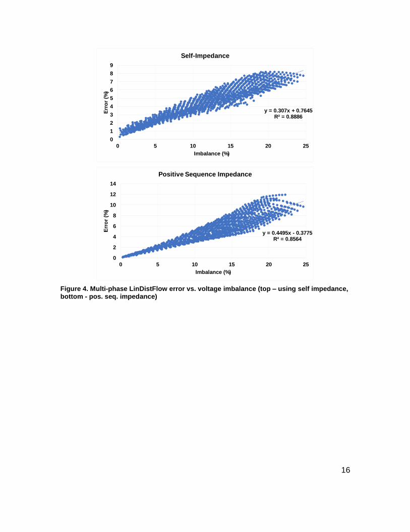
power flow method. Figure 4 gives error versus voltage imbalance, with voltage
imbalance computed as:
16
Figure 4. Multi-phase LinDistFlow error vs. voltage imbalance (top – using self impedance, bottom - pos. seq. impedance)
y = 0.307x + 0.7645R² = 0.8886
0
1
2
3
4
5
6
7
8
9
0 5 10 15 20 25
Err
or
(%)
Imbalance (%)
Self-Impedance
y = 0.4495x - 0.3775R² = 0.8564
0
2
4
6
8
10
12
14
0 5 10 15 20 25
Err
or
(%)
Imbalance (%)
Positive Sequence Impedance

17
𝑉𝑖𝑚𝑏𝑎𝑙𝑎𝑛𝑐𝑒 =
𝑑𝑉𝑚𝑎𝑥
𝑉𝑎𝑣𝑒𝑟𝑎𝑔𝑒 (5)
where 𝑑𝑉𝑚𝑎𝑥 equals the maximum deviated voltage between phases and 𝑉𝑎𝑣𝑒𝑟𝑎𝑔𝑒
is the average voltage at the bus of all phases.
Both self and positive sequence impedances were tested in the voltage
equations and compared for a simple two-bus network. A variety of loading
combinations were applied in order to enumerate through many voltage
imbalance conditions. The top plot shows the error vs. voltage imbalance plot for
the self-impedance term. It can be seen that the maximum error is around 3% for
voltage imbalances less than 5%. The bottom plot shows the results from using
the positive sequence impedance per phase. The maximum error in this case is
around 2% for voltage imbalances less than 5%. It can be numerically observed
that positive sequence impedances provide for a more accurate model for multi-
phase LinDistFlow formulations in the region of minor imbalance. Thus, the
positive sequence impedance term is still kept for each branch voltage equation.
This can be considered an approximation of the self and mutual impedances
given in standard branch impedance matrices. In general, this model should
prove acceptable for market applications, which already assume a relatively
balanced operating point.

18
Robust Optimization
Review of Approaches
As electric power systems integrate more renewable energy resources,
there is added risk in the form of power injection uncertainty. Solar energy
system output, for example, is proportional to solar irradiance, which fluctuates
dynamically over the course of the day. Adverse weather conditions make the
output even more sporadic. This phenomenon, coupled with inherently uncertain
load demand, can create significant randomness in the distribution network that
must be considered in both planning and operations.
In mathematical terms, this entails the modelling of stochastic processes
and the formation of stochastic programs. These types of problems are marked
by parametric randomness in either the objective function or constraints, which in
turn can have significantly different outcomes as compared to their deterministic
forms. The transformation from a deterministic formulation to a stochastic one
can often lead to an entirely new underlying structure (e.g., linear to nonlinear).
Therefore, specific stochastic and/or robust programming methods are usually
needed to properly evaluate them.
Stochastic programming methods generally rely on probability distribution
functions of uncertain data and employ tailored methods that usually consider
decisions made before (ex-ante) and after (ex-post) the uncertain parameter is
actually realized [53]. Expected values are often used for ex-ante stages [53].
Robust programming methods, on the other hand, explicitly incorporate worst
case scenarios in the formulation [54]. Thus, optimal solutions to a robust
optimization problem is itself robust in a technical sense. Robustness as an
attribute is not only attractive, it is often necessary in applied control.
Robust optimization is not new to power systems research and, with the
increase in renewable-based DERs, its incorporation is becoming more and more
prevalent. Several studies incorporate renewable energy uncertainty to solve a
robust economic dispatch problem, e.g. [55] [56] [57]. Some work in this area has
19
also been applied to the unit commitment problem [58]. Naturally, such
approaches have been extended to robust formulations of the OPF problem [59]
[60]. In the context of ADN’s, robust energy management systems have been
developed [61] [62], as well as methods in optimal distributed generation
placement [63].
As previously noted, a robust reformulation of the original problem can
often result in nonlinearities that can make solvability a challenge. In the next
section, a modified interval optimization approach is described that maintains
program linearity.
Interval Optimization Approach
Overview
Uncertain parameters may be modelled in a variety of ways in robust
program development. A robust LP in particular has the following form [64]:
min
{𝑐𝑇𝑥 | 𝐴𝑥 ≤ 𝑏 ∀(𝐴, 𝑏) ∈ 𝑈} (6)
where 𝑈 is the “uncertainty set.” The modelling of uncertain variables comes
down to several factors, including the physical characteristics of the uncertainty,
the discretion of the modeler as well as the tractability of the uncertain
formulation. As further pointed out in [64], expressing uncertainty sets as
ellipsoids results in the transformation of the base LP into a conic quadratic
program which, although slightly more complex, may be solved using standard
quadratic solvers.
Interval variables are another way to model uncertain parameters. An
interval variable consists of an ordered pair of real numbers that represent an
upper and lower bound of a continuous range. Formally, they can be defined as
[65]:
20
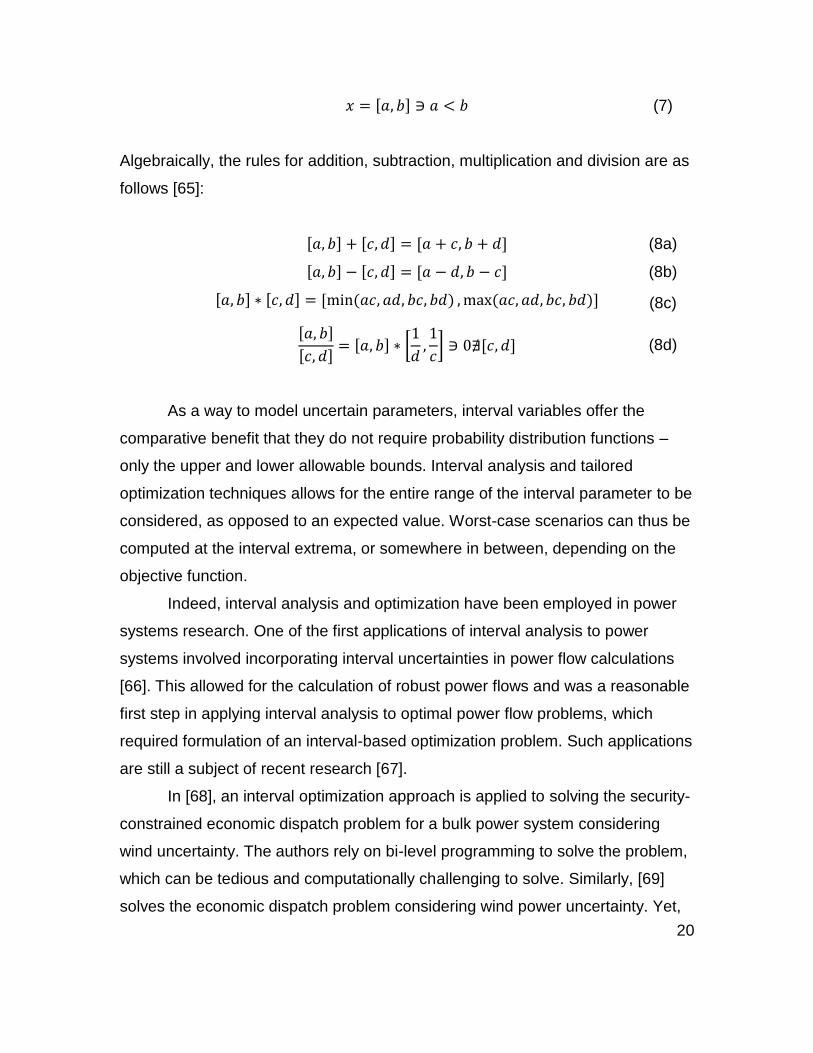
𝑥 = [𝑎, 𝑏] ∋ 𝑎 < 𝑏 (7)
Algebraically, the rules for addition, subtraction, multiplication and division are as
follows [65]:
[𝑎, 𝑏] + [𝑐, 𝑑] = [𝑎 + 𝑐, 𝑏 + 𝑑] (8a)
[𝑎, 𝑏] − [𝑐, 𝑑] = [𝑎 − 𝑑, 𝑏 − 𝑐] (8b)
[𝑎, 𝑏] ∗ [𝑐, 𝑑] = [min
(𝑎𝑐, 𝑎𝑑, 𝑏𝑐, 𝑏𝑑) , max
(𝑎𝑐, 𝑎𝑑, 𝑏𝑐, 𝑏𝑑)] (8c)
[𝑎, 𝑏]
[𝑐, 𝑑]= [𝑎, 𝑏] ∗ [
1
𝑑,1
𝑐] ∋ 0∄[𝑐, 𝑑] (8d)
As a way to model uncertain parameters, interval variables offer the
comparative benefit that they do not require probability distribution functions –
only the upper and lower allowable bounds. Interval analysis and tailored
optimization techniques allows for the entire range of the interval parameter to be
considered, as opposed to an expected value. Worst-case scenarios can thus be
computed at the interval extrema, or somewhere in between, depending on the
objective function.
Indeed, interval analysis and optimization have been employed in power
systems research. One of the first applications of interval analysis to power
systems involved incorporating interval uncertainties in power flow calculations
[66]. This allowed for the calculation of robust power flows and was a reasonable
first step in applying interval analysis to optimal power flow problems, which
required formulation of an interval-based optimization problem. Such applications
are still a subject of recent research [67].
In [68], an interval optimization approach is applied to solving the security-
constrained economic dispatch problem for a bulk power system considering
wind uncertainty. The authors rely on bi-level programming to solve the problem,
which can be tedious and computationally challenging to solve. Similarly, [69]
solves the economic dispatch problem considering wind power uncertainty. Yet,

21
the authors assume that the worst-case occurs only at the extrema of interval
parameters. Reference [70] considers multi-objective microgrid optimization
using interval-based methods, which results in a nonlinear problem and thus
global optimum difficulties.
Enhanced Interval Optimization Development
In this work, an enhanced interval optimization formulation is utilized to
characterize and solve the ADN upper level dispatch problem, given system
uncertainty and nodal flexibility. As will be shown, the end result is a fully linear
formulation, enabling both global optimums to be found as well as the use of off-
the-shelf solvers.
The general interval optimization formulation is developed as [71]:
𝑍 = min𝑥
𝑐𝑖𝑥𝑖 (9a)
𝐴𝑖𝑥𝑖 = [𝑏𝑖, 𝑏𝑖] (9b)
𝐸𝑖𝑥𝑖 ≤ [𝑑𝑖, 𝑑𝑖] (9c)
𝐿𝑖 ≤ 𝑥𝑖 ≤ 𝑈𝑖 (9d)
where a vector of uncertain parameters is given by [𝑏𝑖, 𝑏𝑖] and [𝑑𝑖, 𝑑𝑖].
To solve the problem, first the general formulation (9a)-(9d) is split into two
subproblems [72], representing the best-case (lower bound) and worst-case
(upper bound) solution. The lower bound sub-problem is given by:
𝑍𝑙𝑜𝑤𝑒𝑟 = min𝑥
𝑐𝑖𝑥𝑖 (10a)
𝑏𝑖 ≤ 𝐴𝑖𝑥𝑖 ≤ 𝑏𝑖 (10b)
𝐸𝑖𝑥𝑖 ≤ 𝑑𝑖 (10c)
𝐿𝑖 ≤ 𝑥𝑖 ≤ 𝑈𝑖 (10d)
22
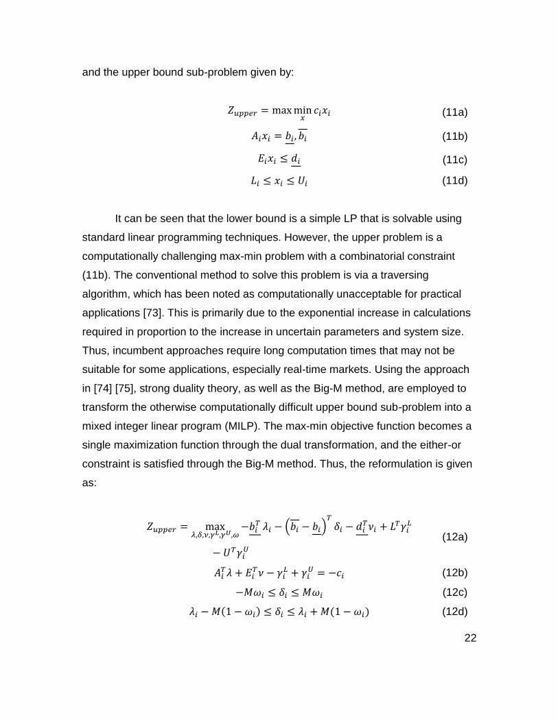
and the upper bound sub-problem given by:
𝑍𝑢𝑝𝑝𝑒𝑟 = max
min𝑥
𝑐𝑖𝑥𝑖 (11a)
𝐴𝑖𝑥𝑖 = 𝑏𝑖, 𝑏𝑖 (11b)
𝐸𝑖𝑥𝑖 ≤ 𝑑𝑖 (11c)
𝐿𝑖 ≤ 𝑥𝑖 ≤ 𝑈𝑖 (11d)
It can be seen that the lower bound is a simple LP that is solvable using
standard linear programming techniques. However, the upper problem is a
computationally challenging max-min problem with a combinatorial constraint
(11b). The conventional method to solve this problem is via a traversing
algorithm, which has been noted as computationally unacceptable for practical
applications [73]. This is primarily due to the exponential increase in calculations
required in proportion to the increase in uncertain parameters and system size.
Thus, incumbent approaches require long computation times that may not be
suitable for some applications, especially real-time markets. Using the approach
in [74] [75], strong duality theory, as well as the Big-M method, are employed to
transform the otherwise computationally difficult upper bound sub-problem into a
mixed integer linear program (MILP). The max-min objective function becomes a
single maximization function through the dual transformation, and the either-or
constraint is satisfied through the Big-M method. Thus, the reformulation is given
as:
𝑍𝑢𝑝𝑝𝑒𝑟 = max
𝜆,𝛿,𝜈,𝛾𝐿,𝛾𝑈,𝜔−𝑏𝑖
𝑇 𝜆𝑖 − (𝑏𝑖 − 𝑏𝑖)𝑇
𝛿𝑖 − 𝑑𝑖𝑇𝜈𝑖 + 𝐿𝑇𝛾𝑖
𝐿
− 𝑈𝑇𝛾𝑖𝑈
(12a)
𝐴𝑖𝑇𝜆 + 𝐸𝑖
𝑇𝜈 − 𝛾𝑖𝐿 + 𝛾𝑖
𝑈 = −𝑐𝑖 (12b)
−𝑀𝜔𝑖 ≤ 𝛿𝑖 ≤ 𝑀𝜔𝑖 (12c)
𝜆𝑖 − 𝑀(1 − 𝜔𝑖) ≤ 𝛿𝑖 ≤ 𝜆𝑖 + 𝑀(1 − 𝜔𝑖) (12d)

23
𝜈𝑖 ≥ 0; 𝛾𝑖𝐿 ≥ 0; 𝛾𝑖
𝑈 ≥ 0; 𝜔𝑖 = 0,1 (12e)
As the reformulation results in a single MILP, it can be given to standard
solvers, which results in a significant computational improvement to the
traversing algorithm, as noted in [74]. In practice, the optimal decision points can
be taken from the reformulated upper bound sub-problem, which represent the
robust solution. The computational improvement allows for this approach to be
employed in an intraday market context, as will be shown in the Chapter III.

24
CHAPTER II HVAC FLEET CONTROL

25
Home Thermal Modelling
As noted previously, system flexibility in this work is engaged through the
aggregation of home HVAC units. Several studies use dynamic models of
various detail, e.g. [76] [77] [78], to describe home thermal behavior, and the
following widely accepted approach is adopted in this study:
𝑡𝑒𝑚𝑝𝑖,𝑡+1𝑖𝑛 = 𝑎 ∗ 𝑡𝑒𝑚𝑝𝑖,𝑡
𝑖𝑛 + 𝑏 ∗ 𝑢𝑖,𝑡ℎ𝑣𝑎𝑐 + 𝑔 ∗ 𝑡𝑒𝑚𝑝𝑡
𝑜𝑢𝑡 (13)
where 𝑡𝑒𝑚𝑝𝑖,𝑡𝑖𝑛 is the indoor temperature of house 𝑖 at time 𝑡; 𝑢𝑖,𝑡
ℎ𝑣𝑎𝑐 is the on/off
status of the HVAC unit 𝑖 at time 𝑡; and 𝑡𝑒𝑚𝑝𝑡𝑜𝑢𝑡 is the outdoor temperature at
time 𝑡. Note that the 𝑢𝑖,𝑡ℎ𝑣𝑎𝑐 term is assumed binary in this work, representative of
residential home HVAC units. The parameters 𝑎, 𝑏, and 𝑔 uniquely describe the
thermal dynamics of each home, and can be determined in a number of ways.
In this work, a system identification approach is used to develop home
thermal models for each house. In system identification, a least squares problem
is computed that parameterizes a pre-determined model, i.e. eqn. (13), with real
data. Input data to develop each home thermal equation came from
corresponding GridLAB-D house objects, which use highly detailed physical
models [79].
Although measurement data sample times may vary depending on the
application, house models for this study were developed from three-minute
samples over a multiple-hour window. This sampling approach is suitable to
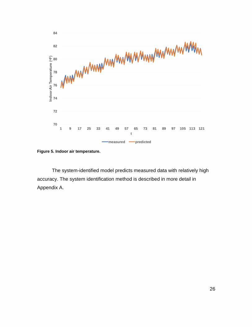
capture the essential dynamics of HVAC units. Figure 5 gives “measured” indoor
air temperature data of a GridLAB-D house object, as well as what was predicted
via the system identification approach (note that the temperature setpoint was
not constant in this simulation).
26
Figure 5. Indoor air temperature.
The system-identified model predicts measured data with relatively high
accuracy. The system identification method is described in more detail in
Appendix A.
70
72
74
76
78
80
82
84
1 9 17 25 33 41 49 57 65 73 81 89 97 105 113 121
Ind
oo
r A
ir T
em
pera
ture
(ᵒF
)
t
measured predicted

27
Model Predictive Control Approach
Classical Approach
MPC is a modern control strategy that utilizes dynamic plant models to
control a process [80]. In an MPC implementation, the controller optimizes the
control input for the current timeslot while taking into account predicted
disturbances. This is known as a “receding horizon” approach.
Classical MPC refers to the control of linear time-invariant (LTI) systems
described by a discrete time model of the form [81]:
𝑥𝑘+𝑡 = 𝐴𝑥𝑘 + 𝐵𝑢𝑘 (14a)
𝑦𝑘 = 𝐶𝑥𝑘 (14b)
where 𝑥𝑘 are system state variables, 𝑢𝑘 are system input variables and 𝑦𝑘 are
output (measurement) variables. States and inputs are also typically constrained:
𝐹𝑥 + 𝐺𝑢 ≤ 𝟏 (15)
The classical regulation problem consists of the design of a controller that
drives the system state to a reference point using some amount of control effort
[81]. Thus, the general objective function is given by [81]:
𝐽∗(𝑥𝑘) ≐ min𝑢𝑘,𝑢𝑘+1,…,𝑢𝑘+𝑛
𝐽(𝑥𝑘, {𝑢𝑘, 𝑢𝑘+1, … , 𝑢𝑘+𝑛}) (16)
where 𝐽 assumes the quadratic cost function driven by positive semi-definite
weight matrices 𝑄 and 𝑅:
𝐽(𝑥0, {𝑢0, 𝑢1, 𝑢2 … }) ≐ ∑(‖𝑥𝑘‖𝑄
2 + ‖𝑢𝑘‖𝑅2 )
∞
𝑘=0
(17)

28
In the classical MPC problem, a sequence of inputs is optimally computed
to minimize the objective function over a given time horizon 𝑛, where the first
control point is applied before moving on to the next time step.
MPC has become a popular approach in power systems research to
optimize the operation of several types of plants, including microgrids [82], [83],
home energy management systems [84], [85] and inverter-based devices [86].
Modified Approach
As noted in [87], an MPC controller may be formulated in a number of
ways to drive the system to a reference signal. The objective function in
particular can be designed depending on the intended outcomes, which may be
related to consumer comfort, electricity price, total energy consumption and
others. Alternatively, some of these outcomes may be better formulated into
constraints.
In the MPC approach used in this work, the objective function has been
modified from the classical formulation to drive the HVAC fleet to follow the
reference signal passed down from the upper level network optimizer, which is a
flexible load dispatch quantity. In this formulation, each controller attempts to
minimize a penalty function that is proportional to the deviation of the sum of
HVAC powers from this reference signal. Thus, the modified objective function
has the form:
min𝑠𝑖,𝑘
∑ 𝑃𝑠𝑖,𝑘
ℎ𝑜𝑟
𝑘=1
(18)
where 𝑃 is a constant penalty factor and 𝑠𝑖,𝑘 is the introduced slack variable to
allow some deviation, if necessary. The controller attempts to minimize this
function from current time step 𝑡 = 𝑘 to some user-defined time horizon 𝑡 = 𝑘 +
ℎ𝑜𝑟. The slack variable is then used in the following constraints:

29
𝑝𝑖,𝑘𝑓𝑙
− 𝑠𝑖,𝑘 ≤ 𝑝𝑟𝑎𝑡𝑒𝑑ℎ𝑣𝑎𝑐 ∑ 𝑢𝑖,𝑘
ℎ𝑣𝑎𝑐
𝑛ℎ𝑣𝑎𝑐
𝑖=1
≤ 𝑠𝑖,𝑘 + 𝑝𝑖,𝑘𝑓𝑙
(19a)
𝑠𝑖,𝑘 ≥ 0 (19b)
where 𝑝𝑖,𝑘𝑓𝑙
is the flexible demand signal generated from the upper level; 𝑢𝑖,𝑘ℎ𝑣𝑎𝑐 is
the on/off status of each home; and 𝑝𝑟𝑎𝑡𝑒𝑑ℎ𝑣𝑎𝑐 is the rated real power draw of HVAC
units; in this work, 𝑝𝑟𝑎𝑡𝑒𝑑ℎ𝑣𝑎𝑐 is assumed to be 4.0 kW, a typical rating for residential
HVAC units. Additional constraints in the MPC function include each home
thermal model (13) as well as upper and lower bounds on indoor air temperature.
This modified formulation produces an MILP instead of the quadratic
program (QP) typically developed in the classical approach.

30
CHAPTER III APPLICATIONS AND DISCUSSION
31
Problem Formulation
Overview
The main application is considered in context of a residential microgrid,
where the operator wishes to drive operational objectives, whilst meeting the
comfort requirements of its customer base. This work assumes that a portion of
the distribution network’s customer base wishes to participate in the electricity
market through an aggregator. To compensate participants, the operator could
pass through realized cost savings via a rebate or credit, for example.
The microgrid operator is able to import power at a locational marginal
price (LMP) of the main substation. The operator can also dispatch flexible power
depending the thermal capabilities of an aggregation of participating HVAC units,
which is coordinated by each nodal HVAC fleet controller. Homes are aggregated
to a bus-phase pair (i.e., node) in the microgrid, and nodes that include
participating HVAC units are called “flexible nodes.”
This is primarily an intraday market application, as the operator makes
optimal decisions at the current timestep, considering a few hours of forecasted
data. The centralized dispatch scheme consists of an upper and lower level,
which are described in the following sections.
Upper Level
The upper level formulates and solves a multi-objective, interval-based
DOPF, which attempts to minimize a weighted cost function of energy
procurement and flexible load dispatch. Problem variables have a time
component associated with them, and the optimizer solves the problem over a
horizon of time steps, taking the current time step solution before re-iterating.
Similar to the receding horizon approach used in MPC, the upper level also
considers forecast data to give it some anticipative ability. This allows the
optimizer to consider future conditions, e.g., high renewable generation output
and/or inflexible load demand. Thus, the objective function has the following
form:

32
min𝑝
𝑖𝑔
,𝑝𝑖𝑓𝑙
∑ ∑ 𝑐𝑖,𝑡𝑔
𝑝𝑖,𝑡𝑔
𝑛𝑔
𝑖=1
ℎ𝑜𝑟
𝑡=𝑘
− ∑ ∑ 𝜔𝑖𝑐𝑖,𝑡𝑓𝑙
𝑝𝑖,𝑡𝑓𝑙
𝑛𝑓
𝑖=1
ℎ𝑜𝑟
𝑡=𝑘
(20)
where 𝑝𝑖,𝑡𝑔
is the real power generation at generation node 𝑖 (this includes power
import at the main substation) at time 𝑡; 𝑝𝑖,𝑡𝑓𝑙
is the dispatchable load at flexible
node 𝑖 at time 𝑡; 𝑐𝑖,𝑡𝑔
cost of generation at generation node 𝑖 at time 𝑡; 𝑐𝑖,𝑡𝑓𝑙
is the
“cost” of flexible load dispatch at flexible node 𝑖 at time 𝑡; and 𝜔𝑖 is the comfort
weight factor at flexible node 𝑖. The variation in weights means that nodes may
be allocated energy differently throughout the dispatch period.
The objective function is combined with the multi-phase LinDistFlow model
given in (4a)-(4c) to produce power balance and nodal voltage equality
constraints for each phase. Further, each phase is coupled through voltage
balance inequalities:
|𝑉𝑖𝑎𝑛 − 𝑉𝑖
𝑏𝑛| ≤ 𝐾 (21a)
|𝑉𝑖𝑏𝑛 − 𝑉𝑖
𝑐𝑛| ≤ 𝐾 (21b)
|𝑉𝑖𝑐𝑛 − 𝑉𝑖
𝑎𝑛| ≤ 𝐾 (21c)
where 𝑉𝑖𝑑𝑛 is the line-to-neutral voltage of phase 𝑑, and 𝐾 is a constant that is set
by the operator. In this work, 𝐾 is taken to be 0.025 (2.5%), which is a standard
voltage imbalance limitation [88]. As will be shown in the Case Study section,
these inequalities help drive voltage (and power) balance throughout the
network.
Nodal power injections are broken down into generation and load
components, which are further broken down into dispatchable and non-
dispatchable terms. Dispatchable terms are decision variables in the optimization
33
problem. Thus, the following equation is used to model real power node injection
(only real power dispatch is considered in this work):
𝑝𝑖,𝑡𝑖𝑛𝑗
= 𝑝𝑖,𝑡𝑔
+ 𝑝𝑖,𝑡𝑟𝑒 − 𝑝𝑖,𝑡
𝑑 − 𝑝𝑖,𝑡𝑓𝑙
(22)
where 𝑝𝑖,𝑡𝑔
is any dispatchable generation at node 𝑖 at time 𝑡; 𝑝𝑖,𝑡𝑟𝑒is renewable
injection at node 𝑖 (this is given as an uncertain interval variable) at time 𝑡; 𝑝𝑖,𝑡𝑑 is
inflexible load demand at node 𝑖 at time 𝑡; and 𝑝𝑖,𝑡𝑓𝑙
represents the dispatchable
demand term at node 𝑖 at time 𝑡. Reactive power loads are modeled as simple
inflexible injections.
All variables are subject to usual upper and lower bounds:
𝑝𝑖𝑔_𝑚𝑖𝑛
≤ 𝑝𝑖𝑔
≤ 𝑝𝑖𝑔_𝑚𝑎𝑥
(23a)
𝑞𝑖𝑔_𝑚𝑖𝑛
≤ 𝑞𝑖𝑔
≤ 𝑞𝑖𝑔_𝑚𝑎𝑥
(23b)
𝑝𝑖𝑓𝑙_𝑚𝑖𝑛
≤ 𝑝𝑖𝑓𝑙
≤ 𝑝𝑖𝑓𝑙_𝑚𝑎𝑥
(23c)
𝑃𝑖𝑚𝑖𝑛 ≤ 𝑃𝑖 ≤ 𝑃𝑖
𝑚𝑎𝑥 (23d)
𝑉𝑖𝑚𝑖𝑛 ≤ 𝑉𝑖 ≤ 𝑉𝑖
𝑚𝑎𝑥 (23e)
The real and reactive power generation at the main substation have large
bounds to allow the microgrid to import enough power to satisfy load demand.
The branch real power flow is limited by typical thermal constraints and 𝑉𝑖𝑚𝑖𝑛 and
𝑉𝑖𝑚𝑎𝑥 are set at 0.95 and 1.05, respectively.
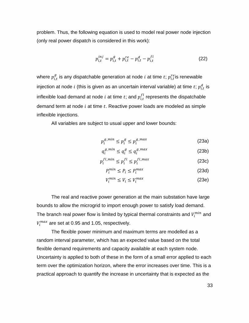
The flexible power minimum and maximum terms are modelled as a
random interval parameter, which has an expected value based on the total
flexible demand requirements and capacity available at each system node.
Uncertainty is applied to both of these in the form of a small error applied to each
term over the optimization horizon, where the error increases over time. This is a
practical approach to quantify the increase in uncertainty that is expected as the
34
outlook of the forecasted parameter increases in time. Figure 6 below portrays
how random parameters are modelled in this work.
Random interval parameters included in the formulation are net inflexible
power injection (i.e., the summation of inflexible load demand and solar power
injection) as well as the flexible power capacities described above.
The full formulation is prepared into the general linear interval optimization
form given in (9a)-(9d), and solved using the enhanced interval optimization
approach described in Chapter I, Section III.
In general, the cost terms can drive a variety of context-dependent
outcomes. Obviously, purely economic goals are already built in: when the cost
to import power (or generate from distributed generators) is greater than the
“cost” to curtail load, then the ADN will attempt to minimize 𝑝𝑖,𝑡𝑓𝑙
terms. In this
Figure 6. Example interval parameter.

35
context, the optimizer is cost-driven. The distribution model will also enable the
ADN to meet operational objectives, like active voltage and power balancing via
flexible load dispatch at system nodes. If voltage optimization is the key
objective, an additional voltage deviation term could be added to the objective
function.
Lower Level
The main design parameters of each controller include sample rate 𝑇𝑠,
control period 𝑇𝑐, and prediction horizon 𝑇𝑝. The sample time describes the rate
at which the controller executes control decisions. The control period is the
number of control decisions made at each iteration, and the prediction horizon is
the range of time that the controller perceives in its computation. The values of
each are listed in Table 1.
This means that, at each dispatch iteration, each fleet controller issues
control points at a three-minute rate over a 15-minute period (i.e., five time
steps), using a prediction horizon of one hour (i.e., 20 time steps). This control
period was designed in order to match the control rate of the upper level, which is
every 15 minutes.
Each fleet controller uses the objective function (18) along with
slack variable constraints described in (19a)-(19b) to compute optimal set points
at each iteration. Also included are each home’s unique thermal model equality
(13), as well as heterogenous upper and lower bounds on indoor air temperature.
Finally, a synchronicity constraint is included to ensure several homes do not
Table 1. Fleet controller design parameters.
Parameter Value
𝑇𝑠 3 min
𝑇𝑐 5 (15 min)
𝑇𝑝 20 (1 hr)

36
simultaneously turn on or off to cause power spikes. This constraint is developed
as:
𝑠𝑦𝑛𝑐𝑖𝑚𝑖𝑛 ≤
∑ 𝑢𝑖,𝑘ℎ𝑣𝑎𝑐ℎ𝑜𝑚𝑒𝑠𝑖
𝑡𝑜𝑡𝑎𝑙
𝑛=1
ℎ𝑜𝑚𝑒𝑠𝑖𝑡𝑜𝑡𝑎𝑙
⁄ ≤ 𝑠𝑦𝑛𝑐𝑖𝑚𝑎𝑥 (24)
where 𝑠𝑦𝑛𝑐𝑖𝑚𝑖𝑛 and 𝑠𝑦𝑛𝑐𝑖
𝑚𝑎𝑥 are fractions between 0-1 that limit simultaneous
minimum and maximum HVAC on status, respectively.
The output of each controller includes a sequence of HVAC set points at
each participating home, as well as updated bounds on the amount of flexible
load (i.e., 𝑝𝑖,𝑡𝑓𝑙_𝑚𝑖𝑛
and 𝑝𝑖,𝑡𝑓𝑙_𝑚𝑎𝑥
) that can be dispatched by the operator over its
next optimization horizon. The maximum capacity term is simply estimated from
the maximum amount of power that can be absorbed by the aggregation of
homes at each node. Likewise, the minimum amount of flexible load required is
an estimation based on minimum power required to maintain an acceptable level
of comfort at each flexible node. As noted previously, these upper and lower
bounds are converted into an uncertain interval parameter for use in the upper
level robust DOPF procedure.
The temporal interaction between the upper and lower levels is described
in the subsequent section.
37
Solution Approach
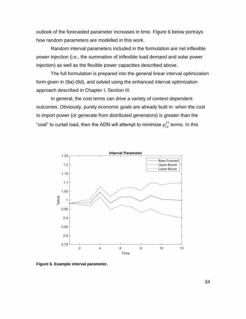
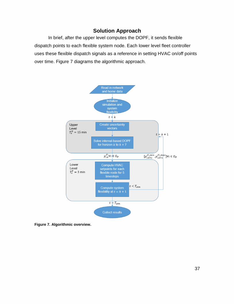
In brief, after the upper level computes the DOPF, it sends flexible
dispatch points to each flexible system node. Each lower level fleet controller
uses these flexible dispatch signals as a reference in setting HVAC on/off points
over time. Figure 7 diagrams the algorithmic approach.
Figure 7. Algorithmic overview.
38
The upper level solves every 15 minutes using a three-hour time horizon.
Each fleet controller then uses 15-minute flexible load dispatch signals over a
one-hour time horizon to optimize three-minute HVAC set points over that period.
Each lower level controller then updates the network optimizer with 𝑝𝑖,𝑡𝑓𝑙_𝑚𝑖𝑛
and
𝑝𝑖,𝑡𝑓𝑙_𝑚𝑎𝑥
terms before the next iteration. Figure 8 portrays a timeline of the
hierarchical control approach.
The algorithm can be applied and started at any point in a simulation, so
long as system data is valid and in appropriate form. Thus, the approach can be
considered a “rolling window” optimization procedure.
Figure 8. Temporal overview of control hierarchy.
39
Case Study
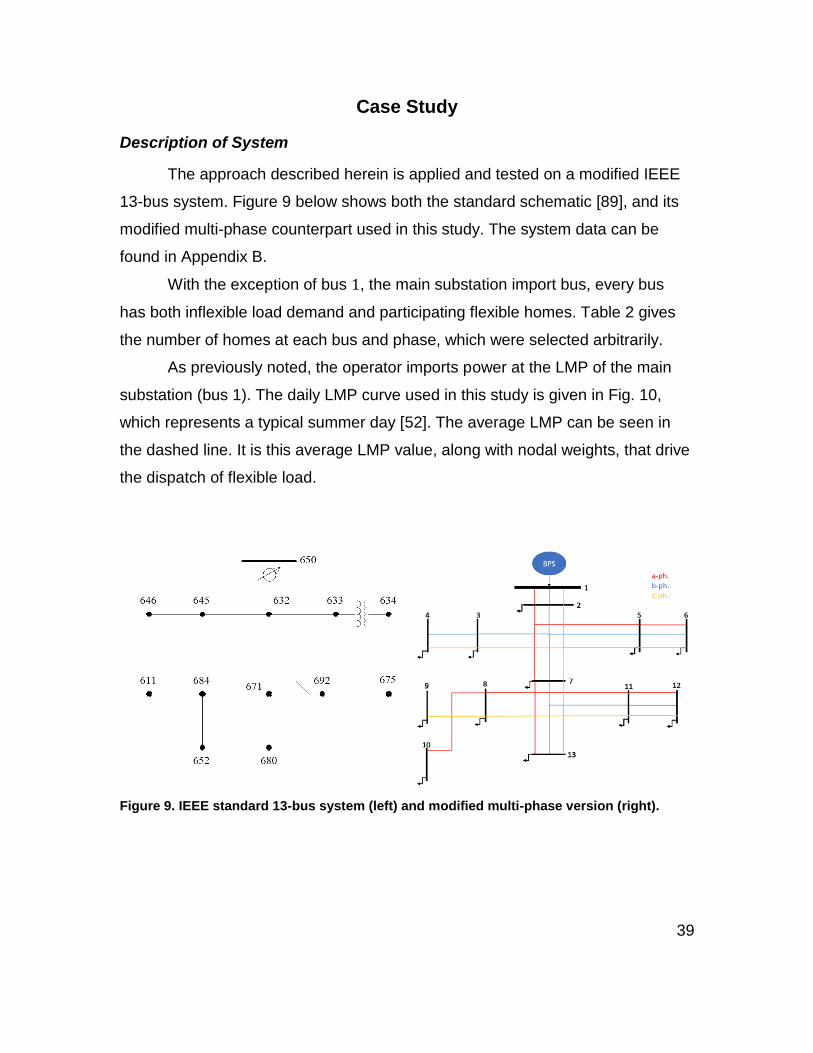
Description of System
The approach described herein is applied and tested on a modified IEEE
13-bus system. Figure 9 below shows both the standard schematic [89], and its
modified multi-phase counterpart used in this study. The system data can be
found in Appendix B.
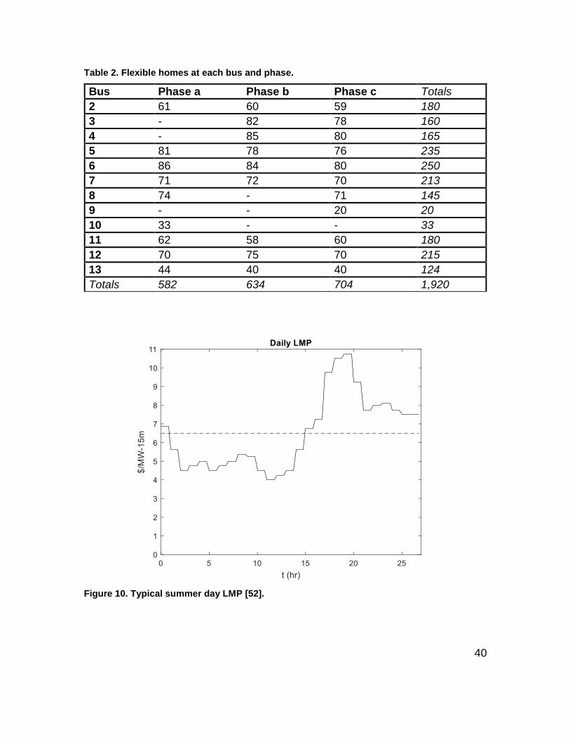
With the exception of bus 1, the main substation import bus, every bus
has both inflexible load demand and participating flexible homes. Table 2 gives
the number of homes at each bus and phase, which were selected arbitrarily.
As previously noted, the operator imports power at the LMP of the main
substation (bus 1). The daily LMP curve used in this study is given in Fig. 10,
which represents a typical summer day [52]. The average LMP can be seen in
the dashed line. It is this average LMP value, along with nodal weights, that drive
the dispatch of flexible load.
Figure 9. IEEE standard 13-bus system (left) and modified multi-phase version (right).
40
Table 2. Flexible homes at each bus and phase.
Bus Phase a Phase b Phase c Totals
2 61 60 59 180
3 - 82 78 160
4 - 85 80 165
5 81 78 76 235
6 86 84 80 250
7 71 72 70 213
8 74 - 71 145
9 - - 20 20
10 33 - - 33
11 62 58 60 180
12 70 75 70 215
13 44 40 40 124
Totals 582 634 704 1,920
Figure 10. Typical summer day LMP [52].
41
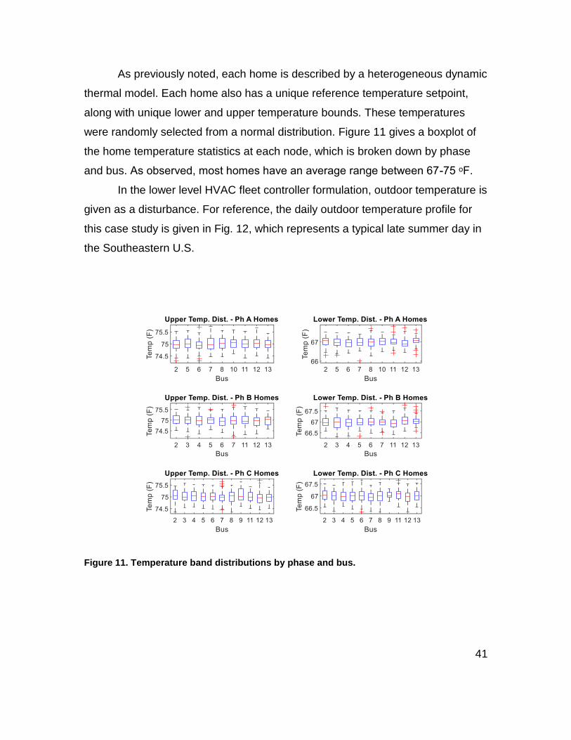
As previously noted, each home is described by a heterogeneous dynamic
thermal model. Each home also has a unique reference temperature setpoint,
along with unique lower and upper temperature bounds. These temperatures
were randomly selected from a normal distribution. Figure 11 gives a boxplot of
the home temperature statistics at each node, which is broken down by phase
and bus. As observed, most homes have an average range between 67-75 ᵒF.
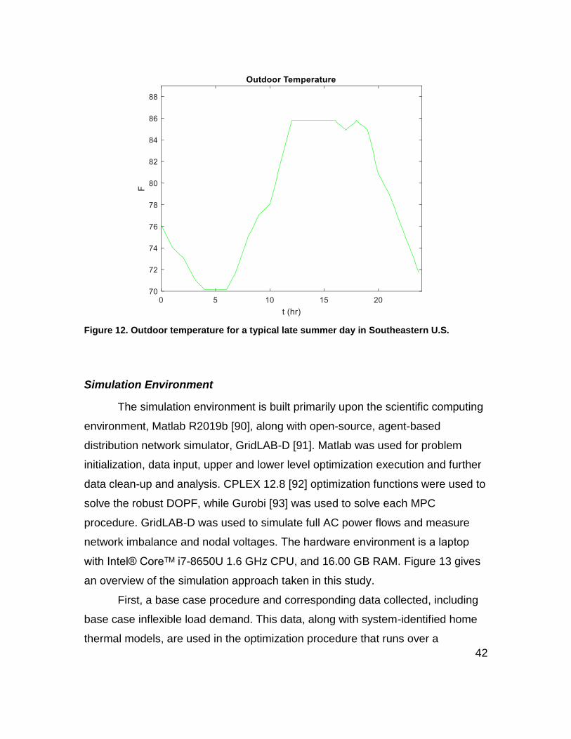
In the lower level HVAC fleet controller formulation, outdoor temperature is
given as a disturbance. For reference, the daily outdoor temperature profile for
this case study is given in Fig. 12, which represents a typical late summer day in
the Southeastern U.S.
Figure 11. Temperature band distributions by phase and bus.
42
Figure 12. Outdoor temperature for a typical late summer day in Southeastern U.S.
Simulation Environment
The simulation environment is built primarily upon the scientific computing
environment, Matlab R2019b [90], along with open-source, agent-based
distribution network simulator, GridLAB-D [91]. Matlab was used for problem
initialization, data input, upper and lower level optimization execution and further
data clean-up and analysis. CPLEX 12.8 [92] optimization functions were used to
solve the robust DOPF, while Gurobi [93] was used to solve each MPC
procedure. GridLAB-D was used to simulate full AC power flows and measure
network imbalance and nodal voltages. The hardware environment is a laptop
with Intel® Coreᵀᴹ i7-8650U 1.6 GHz CPU, and 16.00 GB RAM. Figure 13 gives
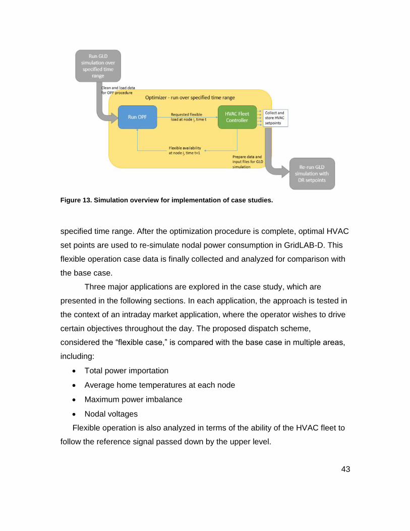
an overview of the simulation approach taken in this study.
First, a base case procedure and corresponding data collected, including
base case inflexible load demand. This data, along with system-identified home
thermal models, are used in the optimization procedure that runs over a
43
Figure 13. Simulation overview for implementation of case studies.
specified time range. After the optimization procedure is complete, optimal HVAC
set points are used to re-simulate nodal power consumption in GridLAB-D. This
flexible operation case data is finally collected and analyzed for comparison with
the base case.
Three major applications are explored in the case study, which are
presented in the following sections. In each application, the approach is tested in
the context of an intraday market application, where the operator wishes to drive
certain objectives throughout the day. The proposed dispatch scheme,
considered the “flexible case,” is compared with the base case in multiple areas,
including:
• Total power importation
• Average home temperatures at each node
• Maximum power imbalance
• Nodal voltages
Flexible operation is also analyzed in terms of the ability of the HVAC fleet to
follow the reference signal passed down by the upper level.
44
Application 1. Load Shaping, Peak Reduction
In the first application, the microgrid operator wishes to shape total load
demand throughout the day to reduce the network peak. The operator
accomplishes this through the objective function described in the problem
formulation: as the revenue of flexible load dispatch falls below the cost of power
import, which occurs during the system peak load condition, the operator will
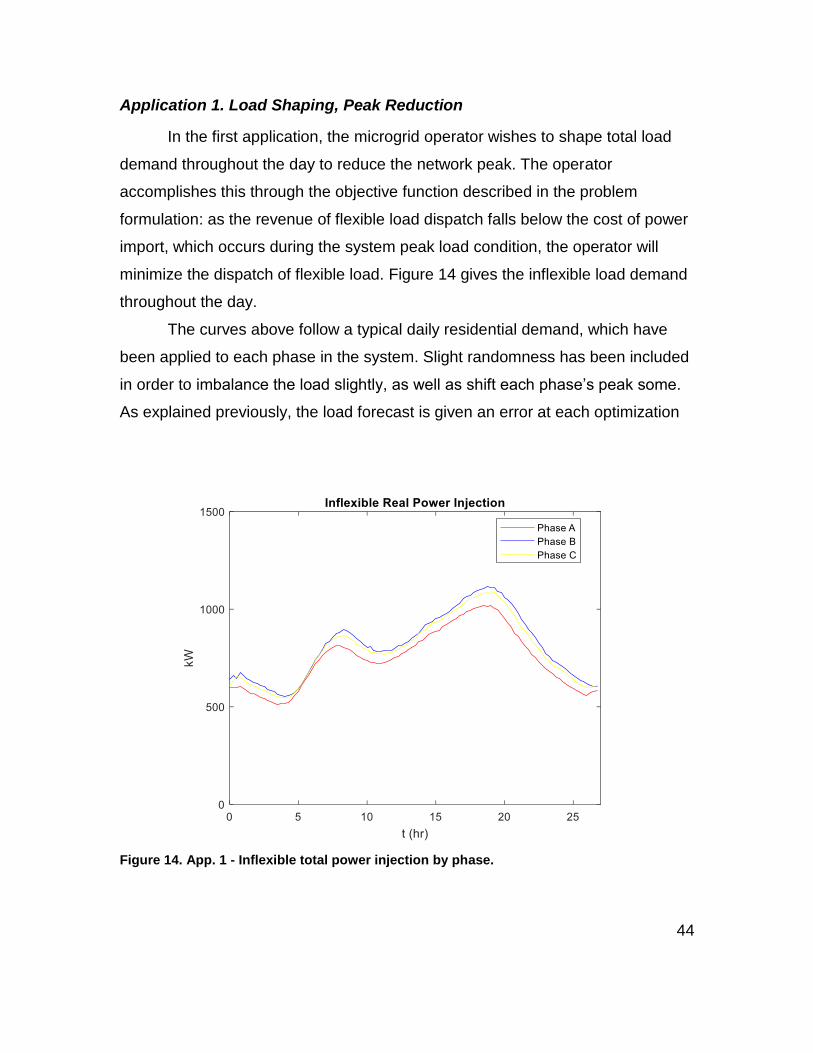
minimize the dispatch of flexible load. Figure 14 gives the inflexible load demand
throughout the day.
The curves above follow a typical daily residential demand, which have
been applied to each phase in the system. Slight randomness has been included
in order to imbalance the load slightly, as well as shift each phase’s peak some.
As explained previously, the load forecast is given an error at each optimization
Figure 14. App. 1 - Inflexible total power injection by phase.
45
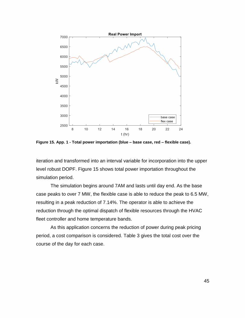
Figure 15. App. 1 - Total power importation (blue – base case, red – flexible case).
iteration and transformed into an interval variable for incorporation into the upper
level robust DOPF. Figure 15 shows total power importation throughout the
simulation period.
The simulation begins around 7AM and lasts until day end. As the base
case peaks to over 7 MW, the flexible case is able to reduce the peak to 6.5 MW,
resulting in a peak reduction of 7.14%. The operator is able to achieve the
reduction through the optimal dispatch of flexible resources through the HVAC
fleet controller and home temperature bands.
As this application concerns the reduction of power during peak pricing
period, a cost comparison is considered. Table 3 gives the total cost over the
course of the day for each case.

46
Table 3. Total cost comparison of base case and flexible case.
Total Cost
Base Case $ 3,539.10
Flexible Case $ 3,115.20
In the base case, peak power occurs over the peak pricing period, which
results in a higher cost. In the flexible case, however, the power is shifted some
from the peak pricing period to the cost shoulders, which results in a total cost
savings of around 12%.
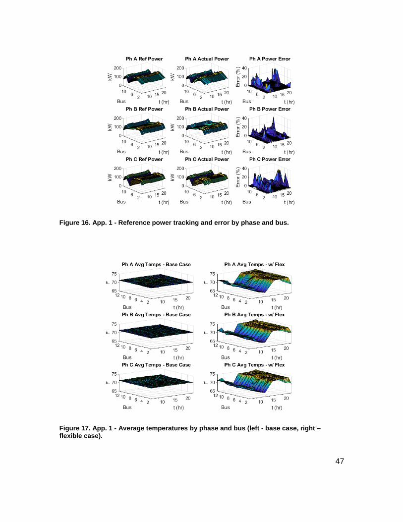
Figure 16 shows three sets of graphs for each phase over the dispatch
period: the left is the reference signal given by the upper level; the middle is the
actual power consumption; the right is the percentage error between the
reference and actual power consumption.
The reference power at each node throughout the simulation equals the
optimal flexible dispatch that is computed by the upper level. During the first few
hours, the upper level allows for maximum power allocation during the off-peak
period, which allows the homes to charge (i.e., cool). During the peak period, the
reference signal drops to a minimal value, which drives the aggregated power
consumption to a lower value. Finally, after the peak period, the signal is
increased to allow the homes to re-charge.
The HVAC fleets are able to track the reference signal with a maximum
error of around 30%. The error is due to the thermal capabilities of each HVAC
fleet. As each fleet nears its upper or lower bound, its ability to dispatch exactly in
line with the upper level reference signal diminishes. The average temperatures
for each bus and phase are shown in Fig. 17.
47
Figure 16. App. 1 - Reference power tracking and error by phase and bus.
Figure 17. App. 1 - Average temperatures by phase and bus (left - base case, right – flexible case).
48
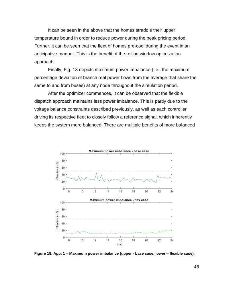
It can be seen in the above that the homes straddle their upper
temperature bound in order to reduce power during the peak pricing period.
Further, it can be seen that the fleet of homes pre-cool during the event in an
anticipative manner. This is the benefit of the rolling window optimization
approach.
Finally, Fig. 18 depicts maximum power imbalance (i.e., the maximum
percentage deviation of branch real power flows from the average that share the
same to and from buses) at any node throughout the simulation period.
After the optimizer commences, it can be observed that the flexible
dispatch approach maintains less power imbalance. This is partly due to the
voltage balance constraints described previously, as well as each controller
driving its respective fleet to closely follow a reference signal, which inherently
keeps the system more balanced. There are multiple benefits of more balanced
Figure 18. App. 1 – Maximum power imbalance (upper - base case, lower – flexible case).
49
operation in a distribution system, including more efficient utilization of tap-
changing transformers and reduced system losses [94].
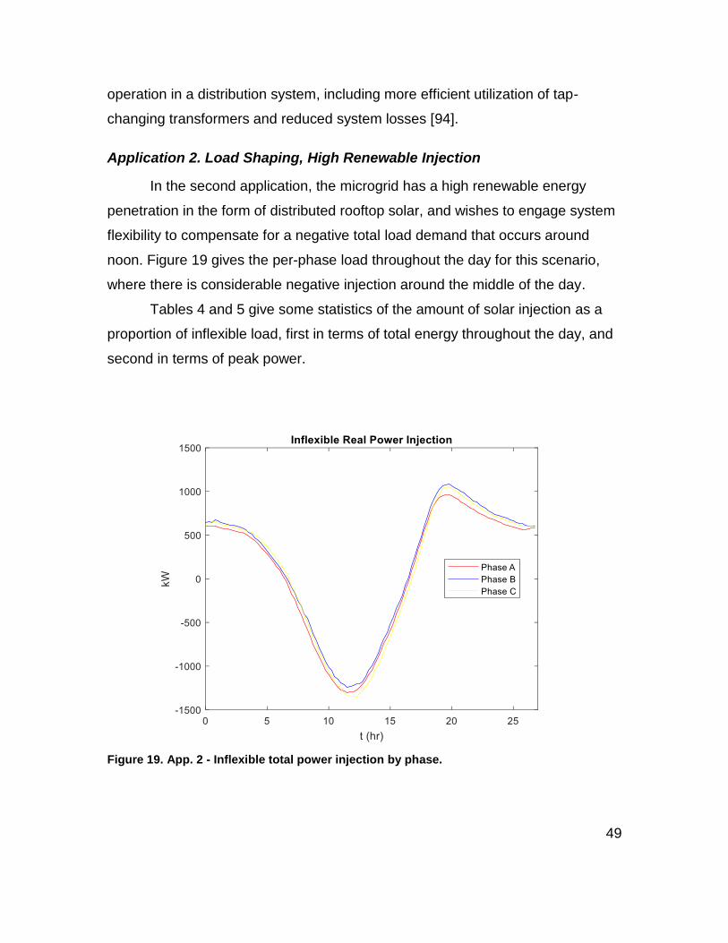
Application 2. Load Shaping, High Renewable Injection
In the second application, the microgrid has a high renewable energy
penetration in the form of distributed rooftop solar, and wishes to engage system
flexibility to compensate for a negative total load demand that occurs around
noon. Figure 19 gives the per-phase load throughout the day for this scenario,
where there is considerable negative injection around the middle of the day.
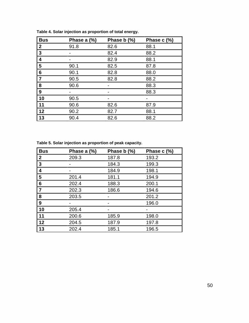
Tables 4 and 5 give some statistics of the amount of solar injection as a
proportion of inflexible load, first in terms of total energy throughout the day, and
second in terms of peak power.
Figure 19. App. 2 - Inflexible total power injection by phase.
50
Table 4. Solar injection as proportion of total energy.
Bus Phase a (%) Phase b (%) Phase c (%)
2 91.8 82.6 88.1
3 - 82.4 88.2
4 - 82.9 88.1
5 90.1 82.5 87.8
6 90.1 82.8 88.0
7 90.5 82.8 88.2
8 90.6 - 88.3
9 - - 88.3
10 90.5 - -
11 90.6 82.6 87.9
12 90.2 82.7 88.1
13 90.4 82.6 88.2
Table 5. Solar injection as proportion of peak capacity.
Bus Phase a (%) Phase b (%) Phase c (%)
2 209.3 187.8 193.2
3 - 184.3 199.3
4 - 184.9 198.1
5 201.4 181.1 194.9
6 202.4 188.3 200.1
7 202.3 186.6 194.6
8 203.5 - 201.2
9 - - 196.0
10 205.4 - -
11 200.6 185.9 198.0
12 204.5 187.9 197.8
13 202.4 185.1 196.5
51
Observably, a large proportion of inflexible load demand can be supplied
through the available solar energy. Yet, most of it occurs around solar noon,
where a lot of it may be lost if not absorbed. This assumes a practical situation in
which the microgrid operator may not be able to export power. Thus, the base
case scenario represents an economic loss for both consumers and the operator.
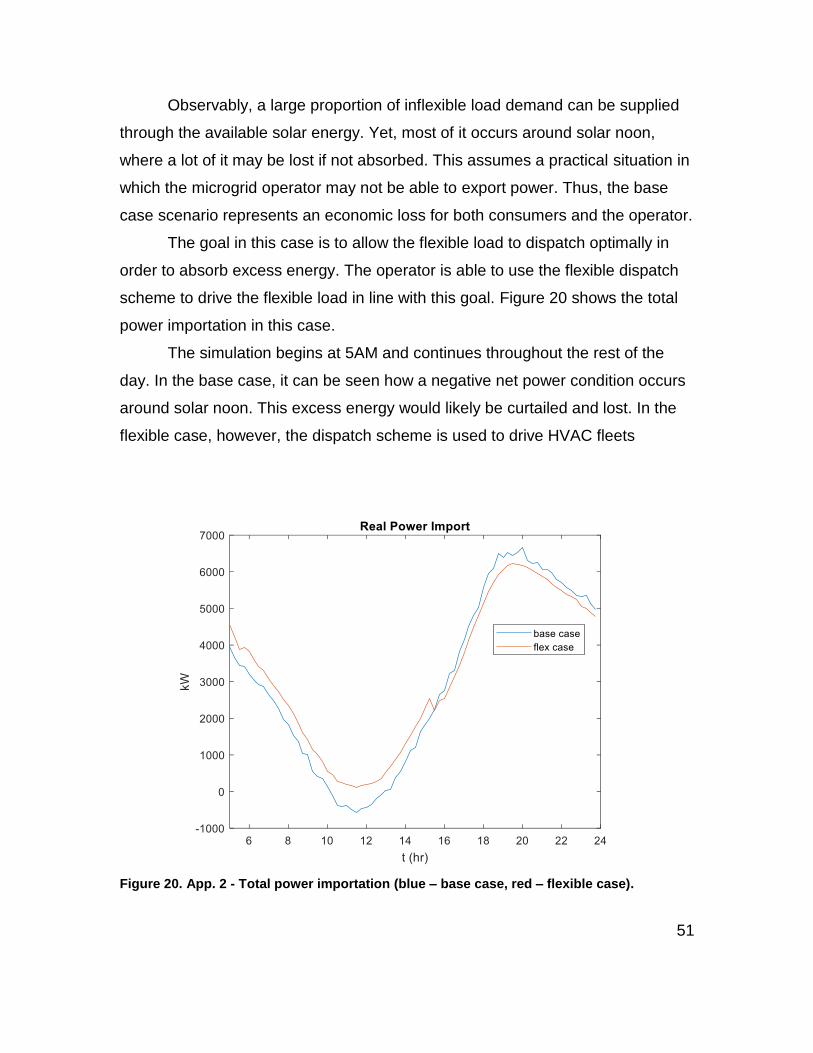
The goal in this case is to allow the flexible load to dispatch optimally in
order to absorb excess energy. The operator is able to use the flexible dispatch
scheme to drive the flexible load in line with this goal. Figure 20 shows the total
power importation in this case.
The simulation begins at 5AM and continues throughout the rest of the
day. In the base case, it can be seen how a negative net power condition occurs
around solar noon. This excess energy would likely be curtailed and lost. In the
flexible case, however, the dispatch scheme is used to drive HVAC fleets
Figure 20. App. 2 - Total power importation (blue – base case, red – flexible case).
52
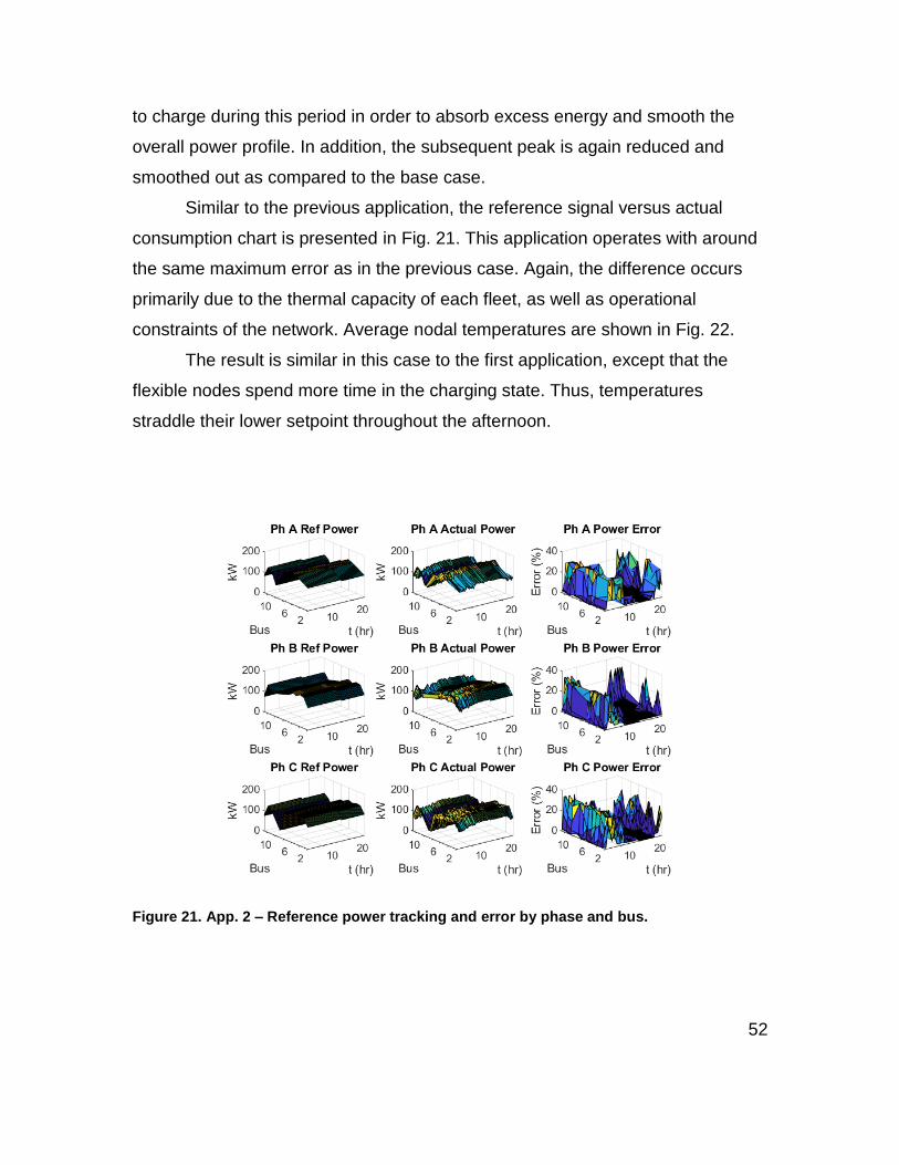
to charge during this period in order to absorb excess energy and smooth the
overall power profile. In addition, the subsequent peak is again reduced and
smoothed out as compared to the base case.
Similar to the previous application, the reference signal versus actual
consumption chart is presented in Fig. 21. This application operates with around
the same maximum error as in the previous case. Again, the difference occurs
primarily due to the thermal capacity of each fleet, as well as operational
constraints of the network. Average nodal temperatures are shown in Fig. 22.
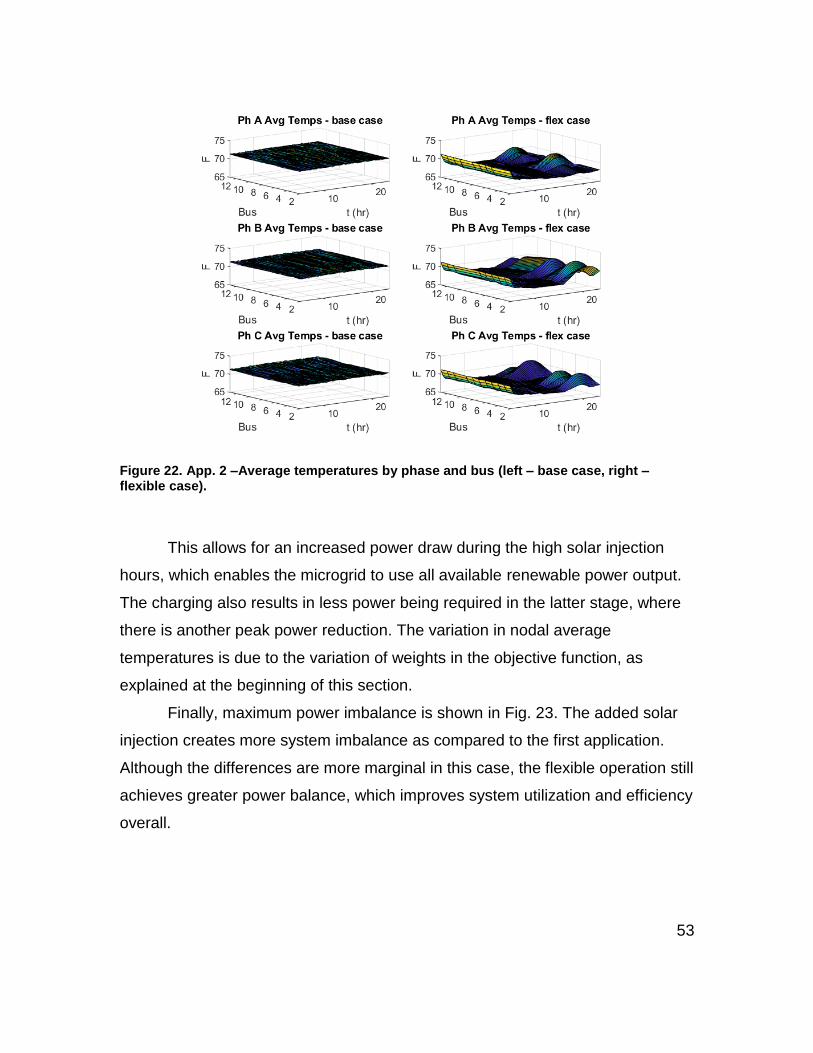
The result is similar in this case to the first application, except that the
flexible nodes spend more time in the charging state. Thus, temperatures
straddle their lower setpoint throughout the afternoon.
Figure 21. App. 2 – Reference power tracking and error by phase and bus.
53
Figure 22. App. 2 –Average temperatures by phase and bus (left – base case, right – flexible case).
This allows for an increased power draw during the high solar injection
hours, which enables the microgrid to use all available renewable power output.
The charging also results in less power being required in the latter stage, where
there is another peak power reduction. The variation in nodal average
temperatures is due to the variation of weights in the objective function, as
explained at the beginning of this section.
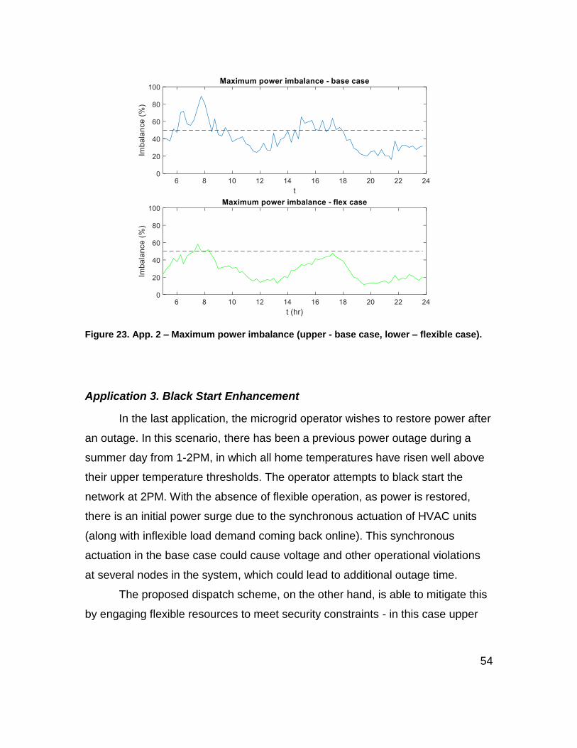
Finally, maximum power imbalance is shown in Fig. 23. The added solar
injection creates more system imbalance as compared to the first application.
Although the differences are more marginal in this case, the flexible operation still
achieves greater power balance, which improves system utilization and efficiency
overall.
54
Figure 23. App. 2 – Maximum power imbalance (upper - base case, lower – flexible case).
Application 3. Black Start Enhancement
In the last application, the microgrid operator wishes to restore power after
an outage. In this scenario, there has been a previous power outage during a
summer day from 1-2PM, in which all home temperatures have risen well above
their upper temperature thresholds. The operator attempts to black start the
network at 2PM. With the absence of flexible operation, as power is restored,
there is an initial power surge due to the synchronous actuation of HVAC units
(along with inflexible load demand coming back online). This synchronous
actuation in the base case could cause voltage and other operational violations
at several nodes in the system, which could lead to additional outage time.
The proposed dispatch scheme, on the other hand, is able to mitigate this
by engaging flexible resources to meet security constraints - in this case upper
55
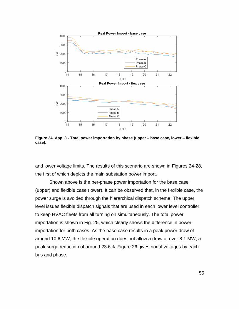
Figure 24. App. 3 - Total power importation by phase (upper – base case, lower – flexible case).
and lower voltage limits. The results of this scenario are shown in Figures 24-28,
the first of which depicts the main substation power import.
Shown above is the per-phase power importation for the base case
(upper) and flexible case (lower). It can be observed that, in the flexible case, the
power surge is avoided through the hierarchical dispatch scheme. The upper
level issues flexible dispatch signals that are used in each lower level controller
to keep HVAC fleets from all turning on simultaneously. The total power
importation is shown in Fig. 25, which clearly shows the difference in power
importation for both cases. As the base case results in a peak power draw of
around 10.6 MW, the flexible operation does not allow a draw of over 8.1 MW, a
peak surge reduction of around 23.6%. Figure 26 gives nodal voltages by each
bus and phase.
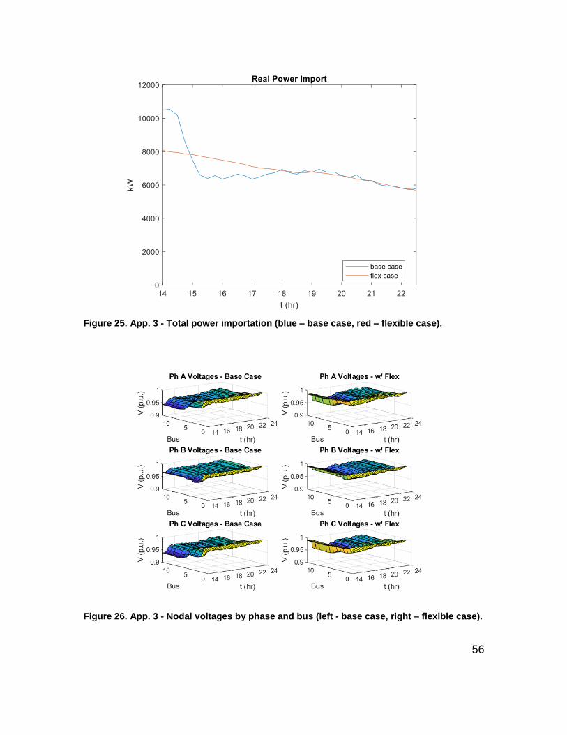
56
Figure 25. App. 3 - Total power importation (blue – base case, red – flexible case).
Figure 26. App. 3 - Nodal voltages by phase and bus (left - base case, right – flexible case).
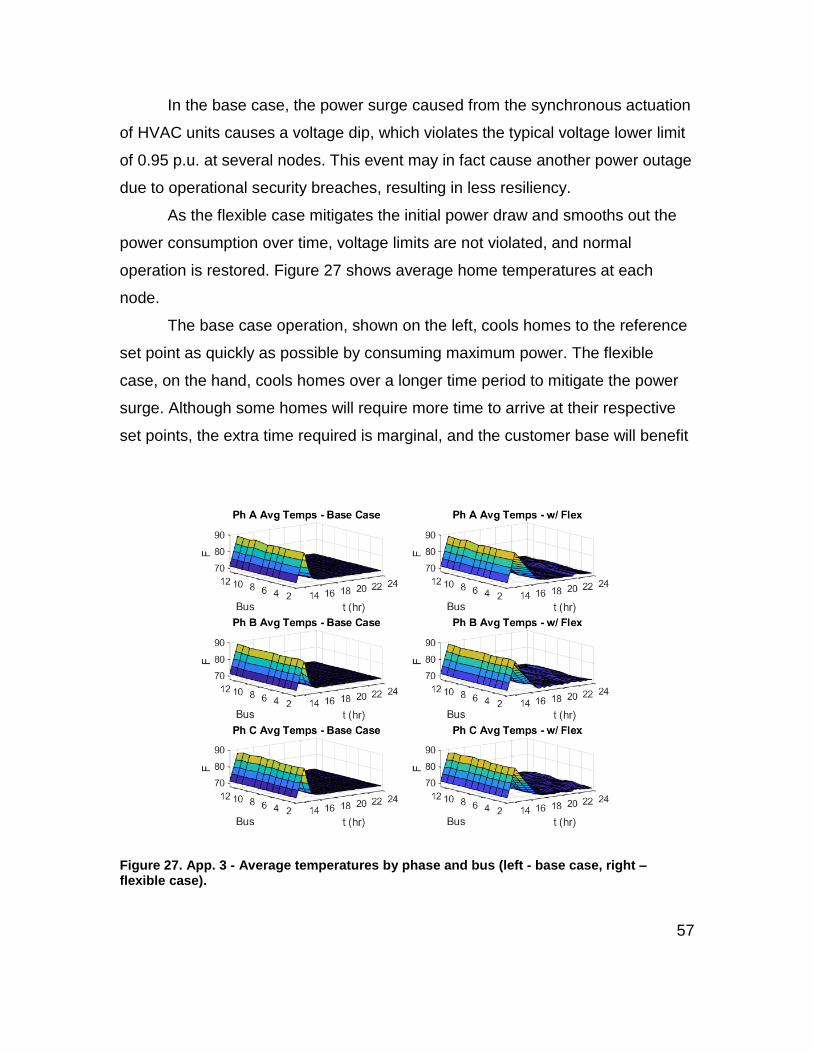
57
In the base case, the power surge caused from the synchronous actuation
of HVAC units causes a voltage dip, which violates the typical voltage lower limit
of 0.95 p.u. at several nodes. This event may in fact cause another power outage
due to operational security breaches, resulting in less resiliency.
As the flexible case mitigates the initial power draw and smooths out the
power consumption over time, voltage limits are not violated, and normal
operation is restored. Figure 27 shows average home temperatures at each
node.
The base case operation, shown on the left, cools homes to the reference
set point as quickly as possible by consuming maximum power. The flexible
case, on the hand, cools homes over a longer time period to mitigate the power
surge. Although some homes will require more time to arrive at their respective
set points, the extra time required is marginal, and the customer base will benefit
Figure 27. App. 3 - Average temperatures by phase and bus (left - base case, right – flexible case).
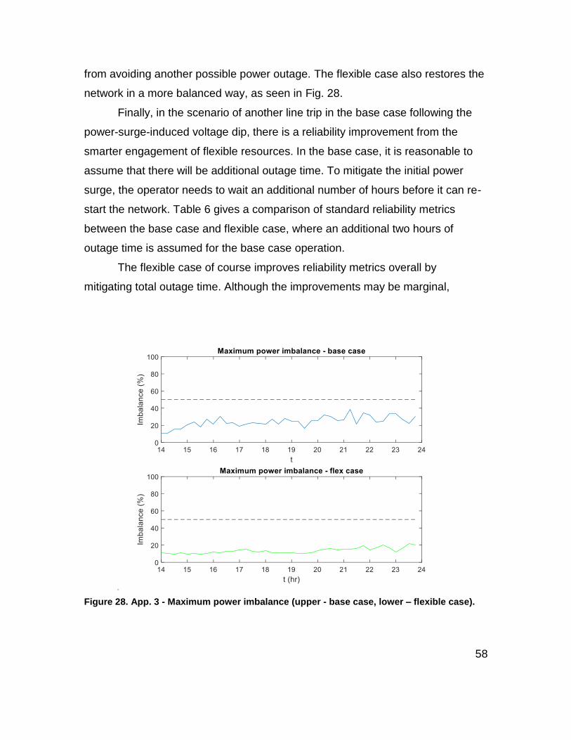
58
from avoiding another possible power outage. The flexible case also restores the
network in a more balanced way, as seen in Fig. 28.
Finally, in the scenario of another line trip in the base case following the
power-surge-induced voltage dip, there is a reliability improvement from the
smarter engagement of flexible resources. In the base case, it is reasonable to
assume that there will be additional outage time. To mitigate the initial power
surge, the operator needs to wait an additional number of hours before it can re-
start the network. Table 6 gives a comparison of standard reliability metrics
between the base case and flexible case, where an additional two hours of
outage time is assumed for the base case operation.
The flexible case of course improves reliability metrics overall by
mitigating total outage time. Although the improvements may be marginal,
Figure 28. App. 3 - Maximum power imbalance (upper - base case, lower – flexible case).

59
increasingly strict power quality standards drive utilities to prevent any network
outages. Thus, incorporating such flexible loads in a black start scenario not only
enhances operation, it may be necessary.
Table 6. Comparison of reliability metrics.
Metric Base Case Flexible Case
SAIDI2 180 mins 60 mins
SAIFI3 2 1
CAIDI4 90 mins 60 mins
ASAI5 99.9486% 99.9886%
2 The system average interruption duration index (SAIDI) is the average duration of a sustained interruption for a customer over some defined period. 3 The system average interruption frequency index (SAIFI) reflects how often the average customer experiences a sustained interruption over some defined period. 4 The customer average interruption duration index (CAIDI) reflects the average time required to restore service for a customer base over a defined period. 5 The average service availability index (ASAI) is the fraction of time that a customer has received power over some defined period.

60
CONCLUSIONS

61
In this thesis, a robust, hierarchical dispatch scheme was presented in the
context of a residential microgrid, which considers thermal flexibility and system
uncertainty. System flexibility is achieved through a participative customer base
that allows for the operation of its HVAC units within a temperature band.
Uncertainty is incorporated in the form of both inflexible nodal real power
injections as well as flexible load capacities.
An enhanced interval optimization approach is used to solve a robust,
multi-phase DOPF at the upper level. The underlying optimization model is
developed from a novel multi-phase LinDistFlow formulation. A rolling-window
approach is formulated in order to consider multiple hours of forecast data. At the
lower level, a modified MPC-based HVAC fleet controller is developed that
controls each participating home at each node. These HVAC fleet controllers
similarly use a horizon of data in order to anticipate both disturbances as well as
the trajectory of the reference signal. The reference signal is passed down to
each flexible node from the upper level, and the lower level sends back flexible
load capacities.
A modified IEEE 13 bus system was used to test the approach in an
intraday market context. Three applications were considered in the case study:
load shaping for peak reduction; load shaping for high renewable penetration;
and a black start scenario. In each case, the flexibility enabled by the approach
allowed for cost reductions, operational benefits and resiliency benefits.
Future work enhancements could be made to this approach. Although the
focus of this work is concerned with home HVAC systems, a number of other
devices could be explored and likely solved with the hierarchical approach. For
example, an ensemble of HVAC units, EVs, and water heaters could be engaged
to follow a reference signal from the upper level optimization procedure. The
author would be interested to explore the dynamical synergies among a number
of flexible energy devices.
Further, the author would like to explore and compare the various
unbalanced distribution models that have and are being developed. Some

62
contexts may require more accuracy than is available from the multi-phase
LinDistFlow approach. Of course, the scheme should also be tested on larger
system sizes, for example the IEEE 123 bus distribution system.
Finally, the author would like to apply the approach in a real-time co-
simulated environment, where the optimization process and network simulator
could be linked and carried out in real time.

63
REFERENCES
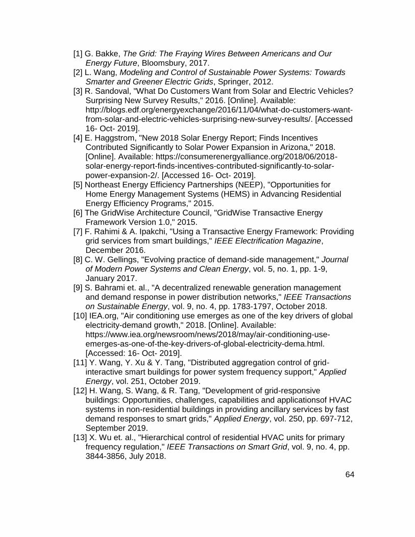
64
[1] G. Bakke, The Grid: The Fraying Wires Between Americans and Our Energy Future, Bloomsbury, 2017.
[2] L. Wang, Modeling and Control of Sustainable Power Systems: Towards Smarter and Greener Electric Grids, Springer, 2012.
[3] R. Sandoval, "What Do Customers Want from Solar and Electric Vehicles? Surprising New Survey Results," 2016. [Online]. Available: http://blogs.edf.org/energyexchange/2016/11/04/what-do-customers-want-from-solar-and-electric-vehicles-surprising-new-survey-results/. [Accessed 16- Oct- 2019].
[4] E. Haggstrom, "New 2018 Solar Energy Report; Finds Incentives Contributed Significantly to Solar Power Expansion in Arizona," 2018. [Online]. Available: https://consumerenergyalliance.org/2018/06/2018-solar-energy-report-finds-incentives-contributed-significantly-to-solar-power-expansion-2/. [Accessed 16- Oct- 2019].
[5] Northeast Energy Efficiency Partnerships (NEEP), "Opportunities for Home Energy Management Systems (HEMS) in Advancing Residential Energy Efficiency Programs," 2015.
[6] The GridWise Architecture Council, "GridWise Transactive Energy Framework Version 1.0," 2015.
[7] F. Rahimi & A. Ipakchi, "Using a Transactive Energy Framework: Providing grid services from smart buildings," IEEE Electrification Magazine, December 2016.
[8] C. W. Gellings, "Evolving practice of demand-side management," Journal of Modern Power Systems and Clean Energy, vol. 5, no. 1, pp. 1-9, January 2017.
[9] S. Bahrami et. al., "A decentralized renewable generation management and demand response in power distribution networks," IEEE Transactions on Sustainable Energy, vol. 9, no. 4, pp. 1783-1797, October 2018.
[10] IEA.org, "Air conditioning use emerges as one of the key drivers of global electricity-demand growth," 2018. [Online]. Available: https://www.iea.org/newsroom/news/2018/may/air-conditioning-use-emerges-as-one-of-the-key-drivers-of-global-electricity-dema.html. [Accessed: 16- Oct- 2019].
[11] Y. Wang, Y. Xu & Y. Tang, "Distributed aggregation control of grid-interactive smart buildings for power system frequency support," Applied Energy, vol. 251, October 2019.
[12] H. Wang, S. Wang, & R. Tang, "Development of grid-responsive buildings: Opportunities, challenges, capabilities and applicationsof HVAC systems in non-residential buildings in providing ancillary services by fast demand responses to smart grids," Applied Energy, vol. 250, pp. 697-712, September 2019.
[13] X. Wu et. al., "Hierarchical control of residential HVAC units for primary frequency regulation," IEEE Transactions on Smart Grid, vol. 9, no. 4, pp. 3844-3856, July 2018.
65
[14] B. Mohandes et. al., "A review of power system flexibility with high penetration of renewables," IEEE Transactions on Power Systems, vol. 34, no. 4, pp. 3140-3155, July 2019.
[15] I. Sami et. al., "A bidirectional interactive electric vehicles operation modes: vehicle-to-grid (V2G) and grid-to-vehicle (G2V) variations within smart grid," in Proc. of International Conference on Engineering and Emerging Technologies, 2019.
[16] H. Turker & I. Colak, "Optimal peak shaving with vehicle-to-grid capability of electric vehicles in smart grids," in Proc. of 7th International Conference on Renewable Energy Research and Applications, 2018.
[17] S. Jaiswal & M. S. Ballal, "Optimal load management of plug-in electric vehicles with demand side management in vehicle to grid application," in Proc. of IEEE Transportation Electrification Conference, 2017.
[18] M. M. Aghdam et. al., "Time-delayed model predictive direct power control for vehicle to grid and grid to vehicle applications," in Proc. of 43rd Annual Conference of the IEEE Industrial Electronics Society, 2017.
[19] M. Ammous, M. Khater & M. AlMuhaini, "Impact of vehicle-to-grid technology on the reliability of distribution systems," in Proc. of 9th IEEE-GCC Conference and Exhibition, 2017.
[20] J. Lei, Z. Xiaoying, Z. Labao & W. Kun, "Coordinating scheduling of electric vehicles and wind power generation considering vehicle to grid mode," in Proc. of IEEE Transportation and Electrification Conference and Expo, 2017.
[21] E. Biyik & A. Kahraman, "A predictive control strategy for optimal management of peak load, thermal comfort, energy storage and renewables in multi-zone buildings," Journal of Building Engineering, vol. 25, September 2019.
[22] S. Kuboth et. al., "Economic model predictive control of combined thermal and electric residential building energy systems," Applied Energy, vol. 240, pp. 372-385, April 2019.
[23] A. F. Taha et. al., "Buildings-to-Grid Integration Framework," IEEE Transactions on Smart Grid, vol. 10, no. 2, pp. 1237-1249, March 2019.
[24] Y. Liu et. al., "Coordinating the operations of smart buildings in smart grids," Applied Energy, vol. 228, pp. 2510-2525, October 2018.
[25] M. Razmara et. al., "Bilevel optimization framework for smart building-to-grid systems," IEEE Transactions on Smart Grid, vol. 9, no. 2, pp. 582-593, March 2018.
[26] A. Mirakhorli & B. Dong, "Model predictive control for building loads connected with a residential distribution grid," Applied Energy, vol. 230, pp. 627-642, November 2018.
[27] A. Hassan et. al., "Optimal load ensemble control in chance-constrained optimal power flow," IEEE Transactions on Smart Grid, vol. 10, no. 5, pp. 5186-5195, September 2019.
66
[28] D. S. Kirschen & G. Strbac, Fundamentals of Power System Economics, First Edition. Wiley, 2004.
[29] A.J. Wood, B.F. Wollenberg & G.B. Sheblé, Power Generation, Operation, and Control, Third Edition. Hoboken, NJ: John Wiley & Sons, 2014.
[30] J.A. Taylor, Convex Optimization of Power Systems. Cambridge, UK: Cambridge University Press, 2015.
[31] J. D. Glover, M. S. Sarma & T. J. Overbye, Power System Analysis and Design, Fifth Edition. Stamford, CT: Cengage Learning, 2012.
[32] M. N. Faqiry & S. Das, "Distributed bilevel energy allocation mechanism with grid constraints and hidden user information," IEEE Transactions on Smart Grid, vol. 10, no. 2, pp. 1869-1879, March 2019.
[33] A. K. Zarabie, S. Das & M. N. Faqiry, "Fairness-regularized DLMP-based bilevel transactive energy mechanism in distribution systems," IEEE Transactions on Smart Grid, In-Press, 2019.
[34] W. Zheng et. al., "A fully distributed reactive power optimization and control method for active distribution networks," IEEE Transactions on Smart Grid, vol. 7, no. 2, pp. 1021-1033, March 2016.
[35] W.H. Kersting, Distribution System Modeling and Analysis, Fourth Edition. Boca Raton, FL: CRC Press, 2017.
[36] F. Xue et. al., "Unbalanced three-phase distribution system power flow with distributed generation using affine arithmetic," in Proc. of 5th International Conference on Electric Utility Deregulation and Restructuring and Power Technologies, 2015.
[37] S. Karagiannopoulos, P. Aristidou & G. Hug, "A centralised control method for tackling unbalances in active distribution grids," in Proc. of Power Systems Computation Conference, 2018.
[38] F. Meng, B. Chowdhury & M. Chamana, "Three-phase optimal power flow for market-based control and optimization of distributed generations," IEEE Transactions on Smart Grid, vol. 9, no. 4, pp. 3691-3700, July 2018.
[39] L. Gan & S. Low, "Convex relaxations and linear approximation for optimal power flow in multiphase radial networks," in Proc. of Power Systems Computation Conference, 2014.
[40] V. Kekatos et. al., "Voltage regulation algorithms for multiphase power distribution grids," IEEE Transactions on Power Systems, vol. 31, no. 5, pp. 3913-3923, September 2016.
[41] Y. Wang et. al., "Linear three-phase power flow for unbalanced active distribution networks with PV nodes," CSEE Journal of Power and Energy Systems, vol. 3, no. 3, pp. 321-324, September 2017.
[42] A. Garces, "A linear three-phase load flow for power distribution systems," IEEE Transactions on Power Systems, vol. 31, no. 1, pp. 827-828, January 2016.
[43] A. Bernstein et. al., “Load flow in multiphase distribution networks: existence, uniqueness,
67
non-singularity and linear models,” IEEE Transactions on Power Systems, vol. 33, no. 6, pp. 5832–5843, November 2018.
[44] S. Hanif et. al., “Multiphase distribution locational marginal prices: approximation and decomposition,” in Proc. of IEEE Power Energy Society General Meeting, 2018.
[45] Y. Liu, J. Li & L. Wu, "Coordinated optimal network reconfiguration and voltage regulator/DER control for unbalanced distribution systems," IEEE Transactions on Smart Grid, vol. 10, no. 3, pp. 2912-2922, May 2019.
[46] H. Ahmadi, J. R. Marti & A. von Meier, "A linear power flow formulation for three-phase distribution systems," IEEE Transactions on Power Systems, vol. 31, no. 6, pp. 5012-5021, November 2016.
[47] M. Baran and F. F. Wu, “Optimal sizing of capacitors placed on a radial distribution system,” IEEE Transactions on Power Delivery, vol. 4, no. 1, pp. 735–743, January 1989.
[48] M. E. Baran & F. F. Wu, "Network reconfiguration in distribution systems for loss reduction and load balancing," IEEE Transactions on Power Delivery, vol. 4, no. 2, pp. 1401-1407, April 1989.
[49] M. Farivar and S. H. Low, “Branch flow model: relaxations and convexification part i,” IEEE Transactions on Power Systems, vol. 28, no. 3, pp. 2554–2564, August 2013.
[50] L. Bai et. al., "Distribution locational marginal pricing (DLMP) for congestion management and voltage support," IEEE Transactions on Power Systems, vol. 33, no. 4, pp. 4061-4073, July 2018.
[51] Wang et. al., "Coordinated energy management of networked microgrids in distribution systems," IEEE Transactions on Smart Grid, vol. 6, no. 1, pp. 45-53, January 2015.
[52] M. Faqiry, et. al., “Transactive-market-based operation of distributed electrical energy storage with grid constraints,” Energies, vol. 10, no. 11, pp. 1-17 , 2017.
[53] J. R. Birge & F. Louveaux, Introduction to Stochastic Programming, Second Edition, Springer, 2011.
[54] A. Ben-Tal & A. Nemirovski, "Robust Convex Optimization," Mathematics of Operations Research, vol. 23, no. 4, pp. 769-805, November 1998.
[55] Z. Tao et. al., "Adjustable robust dynamic economic dispatch of renewable energy considering statistical information," in Proc. of 2nd IEEE Conference on Energy Internet and Energy System Integration, 2018.
[56] M. Zhang, Z. Hu & M. Hu, "Robust economic dispatch considerring wind uncertainty," in Proc. of International Conference on Renewable Power Generation, 2015.
[57] J. Wang & X. Lin, "An economic dispatch method of micro energy grid based on light robust optimization," in Proc. of International Conference on Power System Technology, 2018.
68
[58] D. Bertsimas et. al., "Adapative robust optimization for the security contrained unit commitment problem," IEEE Transactions on Power Systems, vol. 28, no. 1, pp. 52-63, February 2013.
[59] X. Bai, L. Qu & W. Qiao, "Robust AC optimal power flow for power networks with wind power generation," IEEE Transactions on Power Systems, vol. 31, no. 5, pp. 4163-4163, September 2016.
[60] D. Sun et. al., "Robust optimal power flow with transmission switching," in Proc. of 43rd Annual Conference of the IEEE Industrial Electronics Society, 2017.
[61] M. L. Herrera, S. A. Subramanyam & X. Zhang, "Robust control and optimal operation of multiple microgrids with configurable interconnections," in Proc. of IEEE Green Technologies Conference, 2019.
[62] M. Zhai et. al., "Robust model predictive control for energy management of isolated microgrids," in Proc. of IEEE International Conference on Industrial Engineering and Engineering Management, 2017.
[63] Z. Wang et. al., "Robust optimization based optimal DG placement in microgrids," IEEE Transactions on Smart Grid, vol. 5, no. 5, pp. 2173-2182, September 2014.
[64] A. Ben-Tal & A. Nemirovski, "Robust solutions of uncertain linear programs," Operations Research Letters, vol. 25, no. 1, pp. 1-13, August 1999.
[65] M. Abouelsaad et. al., "Assessment of uncertainty in reactive power compensation analysis of distribution systems," in Proc. of Large Engineering Systems Conference on Power Engineering, 2006.
[66] Z. Wang & F. Alvarado, "Interval arithmetic in power flow analysis," in Proc. of Power Industry Computer Application Conference, 1991.
[67] S. S. Parihar & N. Malik, "Interval arithmetic power flow analysis of radial distribution system including uncertainties in input as parameters," in Proc. of 7th International Conference on Power Systems, 2017.
[68] T. Ding, et. al., “Bi-level linear programming based interval optimization for SCED in the presence of wind power uncertainty,” in Proc. of IEEE PES General Meeting Conference & Exposition, July 2014.
[69] H. Ma et. al., "A robust interval economic dispatch method accommodating significant wind power integration," in Proc. of IEEE PES Asia-Pacific Power and Energy Engineering Conference, 2018.
[70] Y. Li, et. al., “Multi-objective optimal dispatch of microgrid under uncertainties via interval optimization,” IEEE Transactions on Smart Grid, vol. 10, no. 2, pp. 2046-2058, March 2019.
[71] T. Ding et. al., "Absolute value constraint based method for interval optimization to SCED model," IEEE Transactions on Power Systems, vol. 29, no. 2, pp. 980-981, March 2014.
[72] L. Bai, F. Li, H. Cui, et. al, “Interval optimization based operating strategy for gas-electricity integrated energy systems considering demand
69
response and wind uncertainty,” Applied Energy, vol. 167, pp. 270-279, Apr. 2016.
[73] X. Kou, F. Li & W. Feng, "Transmission constrained economic dispatch via interval optimization considering wind uncertainty," in Proc. of IEEE Power & Energy Society General Meeting, 2018.
[74] X. Kou & F. Li, "Interval optimization for available transfer capacity (ATC) evaluation considering wind power uncertainty," IEEE Transactions on Sustainable Energy, In-Press, 2019.
[75] C. Rooks, X. Kou & F. Li, “Interval optimization for robust economic dispatch in active distribution networks considering uncertainty,” in Proc. of 2nd International Conference on Smart Energy Systems and Technologies, 2019.
[76] M. Heleno, M. A. Matos & J. A. P. Lopes, "Availability and flexibility of loads for the provision of reserve," IEEE Transactions on Smart Grid, vol. 6, no. 2, pp. 667-674, March 2015.
[77] B. Feron & A. Monti, "Integration of space heating demand flexibility in a home energy management system using a market-based multi agent system," in Proc. of IEEE Power & Energy Society General Meeting, 2017.
[78] X. Jin et. al., "User-preference-driven model predictive control of residential building loads and battery storage for demand response," in Proc. of American Control Conference, 2017.
[79] GridLAB-D Wiki, "Residential module user's guide," 2017. [Online]. Available: http://gridlab-d.shoutwiki.com/wiki/Residential_module_user%27s_guide. [Accessed 16- Oct- 2019].
[80] M. Morari, C. E. Garcia & D. M. Prett, "Model predictive control: Theory and practice," IFAC Proceedings Volumes, vol. 21, no. 4, pp. 1-12, June 1988.
[81] B. Kouvaritakis & M. Cannon, Model Predictive Control: Classical, Robust and Stochastic, Springer, 2016.
[82] A. J. Babqi, Z. Yi & A. H. Etemadi, "Centralized finite control set model predictive control for multiple distributed generator small-scale microgrids," in Proc. of North American Power Symposium, 2017.
[83] B. R. Ravada, N. R. Tummuru, R. Oruganti, "Control of mixed energy storage system based micro-grid using modulator-less model predictive control," in Proc. of International Conference on Power Electronics, Drives and Energy Systems, 2018.
[84] Y. Ogata & T. Namerikawa, "Energy management of smart home by model predictive control based on EV state prediction," in Proc. of 12th Asian Control Conference, 2019.
[85] M. Yousefi et. al., "Smart energy management system for residential homes regarding uncertainties of photovoltaic array and plug-in electric vehicle," in Proc. of IEEE 28th International Symposium on Industrial Electronics, 2019.

70
[86] J. M. C. Geldenhuys et. al., "Model predictive current control of a grid connected converter with LCL-filter," in Proc. of IEEE 17th Workshop on Control and Modeling for Power Electronics," 2016.
[87] A. Mirakhorli & B. Dong, "Occupant-behavior driven appliance scheduling for residential buildings," Building Simulation, vol. 10, no. 6, pp. 917-931, December 2017.
[88] Pacific Gas and Electric Company, "Voltage Unbalance and Motors," 2009. [Online]. Available: https://www.pge.com/includes/docs/pdfs/mybusiness/customerservice/energystatus/powerquality/voltage_unbalance_rev2.pdf. [Accessed 16- Oct- 2019].
[89] K.P. Schneider et. al., "Analytic considerations and design basis for the IEEE Distribution Test Feeders," IEEE Transactions on Power Systems, vol. 33, no. 3, pp. 3181-3188, May 2018.
[90] MATLAB 2019a, The Mathworks, Inc., Natick, Massachusetts, United States.
[91] D. P. Chassin, K. P. Schneider, and C. Gerkensmeyer, “GridLAB-D: An open-source power systems modeling and simulation environment,” in Proc. of IEEE PES Transm. Distrib. Conf. Expo., 2008.
[92] CPLEX 12.8, IBM ILOG, Armonk, New York, United States. [93] Gurobi, Gurobi Optimization, LLC., "Gurobi Optimizer Reference
Manual," 2019. [94] M. R. Vuluvala & L. M. Saini, "Load balancing of electrical power
distribution system: An overview," in Proc. of International Conference on Power, Instrumentation, Control and Computing, 2018.

71
APPENDIX
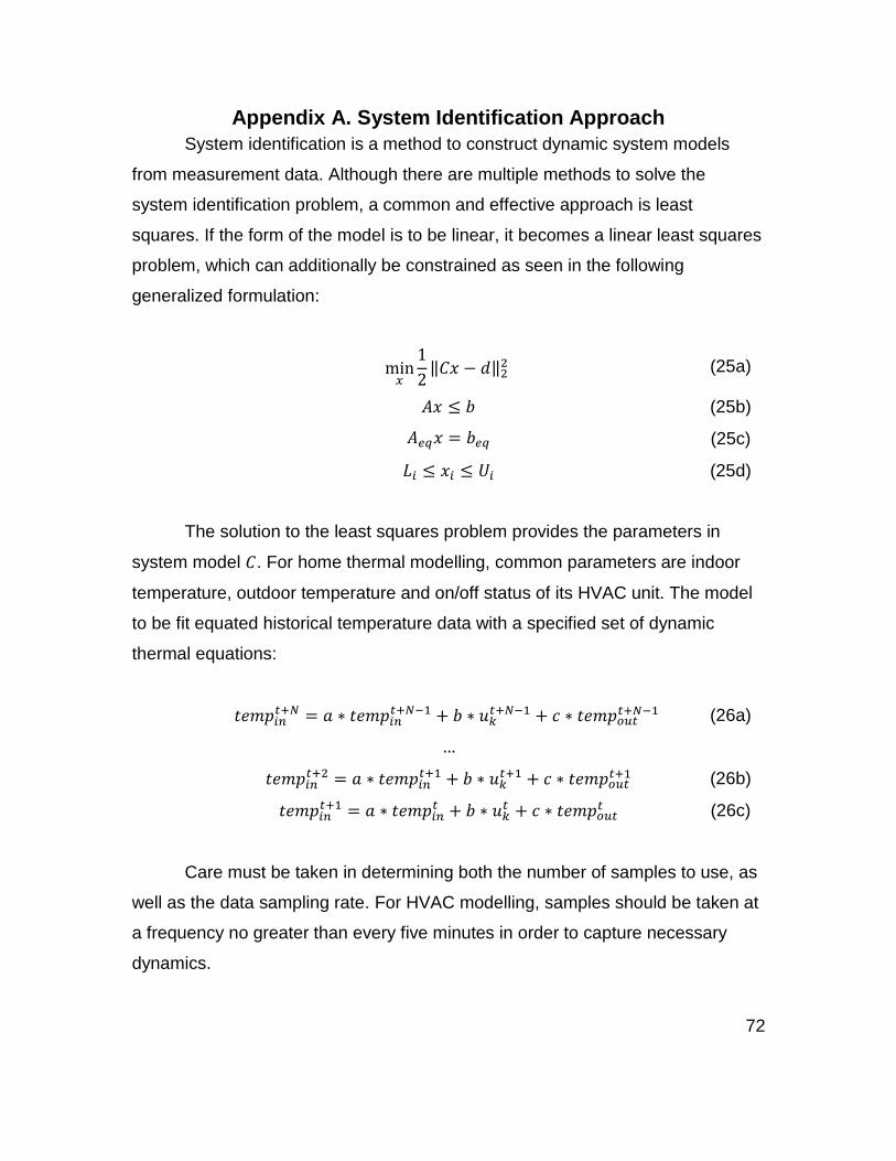
72
Appendix A. System Identification Approach
System identification is a method to construct dynamic system models
from measurement data. Although there are multiple methods to solve the
system identification problem, a common and effective approach is least
squares. If the form of the model is to be linear, it becomes a linear least squares
problem, which can additionally be constrained as seen in the following
generalized formulation:
min
𝑥
1
2‖𝐶𝑥 − 𝑑‖2
2 (25a)
𝐴𝑥 ≤ 𝑏 (25b)
𝐴𝑒𝑞𝑥 = 𝑏𝑒𝑞 (25c)
𝐿𝑖 ≤ 𝑥𝑖 ≤ 𝑈𝑖 (25d)
The solution to the least squares problem provides the parameters in
system model 𝐶. For home thermal modelling, common parameters are indoor
temperature, outdoor temperature and on/off status of its HVAC unit. The model
to be fit equated historical temperature data with a specified set of dynamic
thermal equations:
𝑡𝑒𝑚𝑝𝑖𝑛𝑡+𝑁 = 𝑎 ∗ 𝑡𝑒𝑚𝑝𝑖𝑛
𝑡+𝑁−1 + 𝑏 ∗ 𝑢𝑘𝑡+𝑁−1 + 𝑐 ∗ 𝑡𝑒𝑚𝑝𝑜𝑢𝑡
𝑡+𝑁−1 (26a)
…
𝑡𝑒𝑚𝑝𝑖𝑛𝑡+2 = 𝑎 ∗ 𝑡𝑒𝑚𝑝𝑖𝑛
𝑡+1 + 𝑏 ∗ 𝑢𝑘𝑡+1 + 𝑐 ∗ 𝑡𝑒𝑚𝑝𝑜𝑢𝑡
𝑡+1 (26b)
𝑡𝑒𝑚𝑝𝑖𝑛𝑡+1 = 𝑎 ∗ 𝑡𝑒𝑚𝑝𝑖𝑛
𝑡 + 𝑏 ∗ 𝑢𝑘𝑡 + 𝑐 ∗ 𝑡𝑒𝑚𝑝𝑜𝑢𝑡
𝑡 (26c)
Care must be taken in determining both the number of samples to use, as
well as the data sampling rate. For HVAC modelling, samples should be taken at
a frequency no greater than every five minutes in order to capture necessary
dynamics.
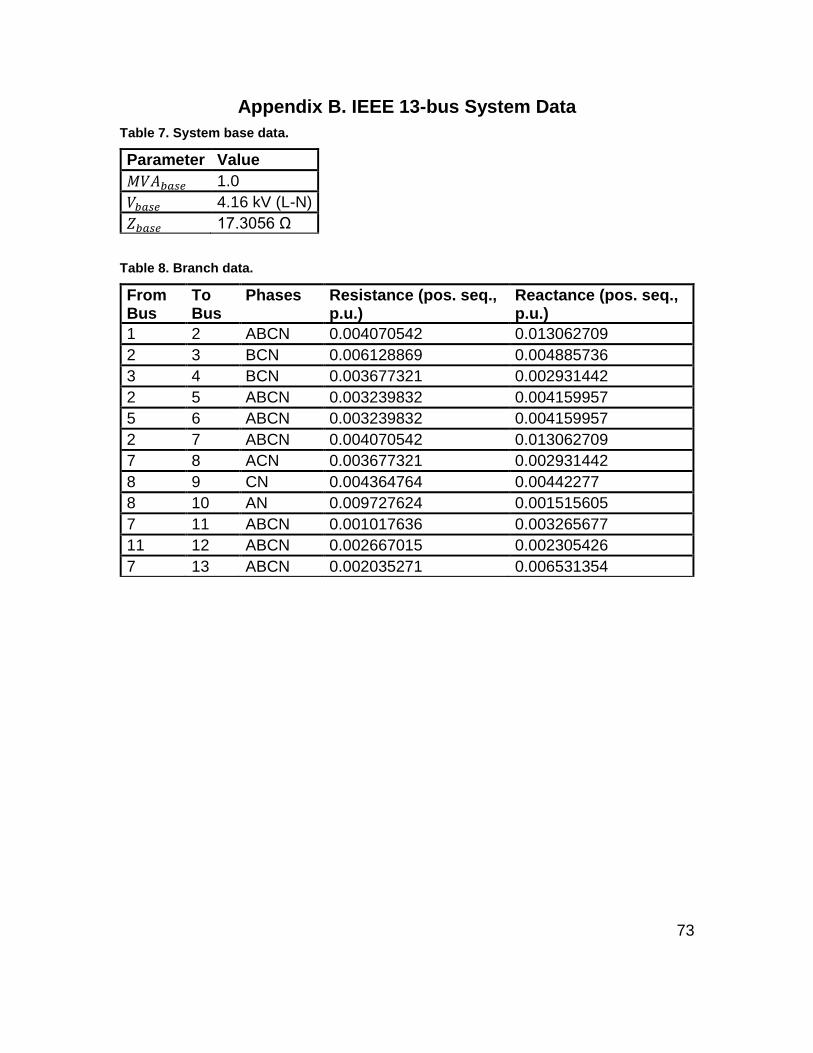
73
Appendix B. IEEE 13-bus System Data
Table 7. System base data.
Parameter Value
𝑀𝑉𝐴𝑏𝑎𝑠𝑒 1.0
𝑉𝑏𝑎𝑠𝑒 4.16 kV (L-N)
𝑍𝑏𝑎𝑠𝑒 17.3056 Ω
Table 8. Branch data.
From Bus
To Bus
Phases Resistance (pos. seq., p.u.)
Reactance (pos. seq., p.u.)
1 2 ABCN 0.004070542 0.013062709
2 3 BCN 0.006128869 0.004885736
3 4 BCN 0.003677321 0.002931442
2 5 ABCN 0.003239832 0.004159957
5 6 ABCN 0.003239832 0.004159957
2 7 ABCN 0.004070542 0.013062709
7 8 ACN 0.003677321 0.002931442
8 9 CN 0.004364764 0.00442277
8 10 AN 0.009727624 0.001515605
7 11 ABCN 0.001017636 0.003265677
11 12 ABCN 0.002667015 0.002305426
7 13 ABCN 0.002035271 0.006531354

74
VITA
Cody Davis Rooks was born in Nashville, Tennessee, USA on February
19, 1990. He received a B.S. degree in Engineering Science from Vanderbilt
University in 2012. He began the M.S. in Electrical Engineering program at the
University of Tennessee, Knoxville in the Fall of 2017 and aims to complete the
program in 2019. His research interests include microgrid design, renewable
energy integration, device-to-grid integration, and power system analysis and
optimization.