A ROBUST NAVIGATION SYSTEM USING GPS, MEMS INERTIAL SENSORS AND RULE-BASED DATA FUSION

A Thesis

Submitted to the Temple University Graduate Board

in Partial Fulfillment of the Requirements for the Degree

MASTER OF SCIENCE IN ENGINEERING

by

Zexi Liu, B.S.E.E.

May, 2009

Chang-Hee Won

Thesis Advisor College of Engineering

Committee Member

Li Bai

College of Engineering Committee Member

Saroj K. Biswas

College of Engineering Committee Member

ii

ABSTRACT

A robust navigation system using a Global Positioning System (GPS) receiver,

Micro-Electro-Mechanical Systems (MEMS) inertial sensors, and rule-based data fusion

has been developed. An inertial measurement unit tends to accumulate errors over time.

A GPS receiver, on the other hand, does not accumulate errors over time, but the

augmentation with other sensors is needed because the GPS receiver fails in stressed

environments such as beneath the buildings, tunnels, forests, and indoors. This limits the

usage of a GPS receiver as a navigation system for automobiles, unmanned vehicles, and

pedestrians. The objective of this project is to augment GPS signals with MEMS inertial

sensor data and a novel data fusion method. A rule-based data fusion concept is used in

this procedure. The algorithm contains knowledge obtained from a human expert and

represents the knowledge in the form of rules. The output of this algorithm is position,

orientation, and attitude. The performance of this mobile experimental platform under

both indoor and outdoor circumstances has been tested. Based on the results of these

tests, a new integrated system has been designed and developed in order to replace the

former system which was assembled by using off-the-shelf devices. In addition, Personal

Navigation System (PNS) has been designed, built, and tested by attaching different

inertial sensors on the human body. This system is designed to track a person in any

motion such as walking, running, going up/down stairs, sitting, and lying down. A series

of experiments have been performed. And the test results are obtained and discussed.

iii

ACKNOWLEDGEMENTS

This Master Thesis project was carried out at the Control, Sensor, Network, and

Perception (CSNAP) Laboratory, Department of Electrical & Computer Engineering, at

the Temple University. I would like to thank my advisor, Dr. Chang-Hee Won, for his

many suggestions and constant support during this research. I am also thankful to my

committee members Dr. Bai and Dr. Biswas for their help, support, and all the

discussions throughout this research.

The help provided by them was crucial to the successful completion of my thesis.

And it was a pleasure to work with them.

Thanks also go to Bei Kang and Jong-Ha Lee from the CSNAP Lab, for the help

with the system design and assembly, and to my friends and fellow students at Temple

University for the enjoyable and nice time here.

Zexi Liu

May, 2009

iv

TABLE OF CONTENTS

ABSTRACT .................................................................................................... ii

ACKNOWLEDGEMENTS ........................................................................... iii

LIST OF FIGURES ....................................................................................... vii

LIST OF TABLES .......................................................................................... xi

CHAPTER

1. INTRODUCTION ..................................................................................... 1

1.1 Introduction ...............................................................................................................1

1.2 Objective ...................................................................................................................2

1.3 Scope of Research and Methodology ........................................................................3

1.4 Organization of the Thesis ........................................................................................4

2. LITERATURE REVIEW ......................................................................... 5

2.1 Introduction ...............................................................................................................5

2.2 Global Positioning System ........................................................................................7

2.3 Inertial Measurement Unit ........................................................................................9

2.4 Reference Frames ....................................................................................................14

2.5 Data Fusion .............................................................................................................20

2.6 Rule-based System ..................................................................................................22

2.7 Personal Navigation System ...................................................................................26

3. MOBILE PLATFORM ........................................................................... 28

3.1 System Overview ....................................................................................................28

3.2 Hardware Design .....................................................................................................30

3.3 Firmware Design .....................................................................................................34

v

4. DATA PROCESSING UNIT .................................................................. 36

4.1 Design Overview .....................................................................................................36

4.2 Rule-based Data Fusion ..........................................................................................41

4.3 Evaluation Method for Data Fusion Results ...........................................................70

5. EXPERIMENTS AND RESULTS DISCUSSION ............................... 73

5.1 Experiment Conditions ............................................................................................73

5.2 Devices ....................................................................................................................76

5.3 Experiment Result Discussion ................................................................................77

5.4 Indoor Experiments .................................................................................................84

6. INTEGRATED SYSTEM DESIGN ...................................................... 88

6.1 Backgrounds ............................................................................................................88

6.2 Top-level Design .....................................................................................................89

6.3 Bill of Materials ......................................................................................................92

6.4 The PCB Layout Design .........................................................................................94

6.5 The Prototype and Conclusions ..............................................................................99

7. PERSONAL NAVIGATION SYSTEM .............................................. 101

7.1 Introduction ...........................................................................................................101

7.2 Method #1 Waist Attached Sensor ........................................................................102

7.3 Method #2 Knee Attached Sensor .........................................................................115

7.4 Method #3 Foot Attached Sensor ..........................................................................125

7.5 Proposed Personal Navigation System and Test Results ......................................131

7.6 Conclusions ...........................................................................................................141

8. CONCLUSIONS .................................................................................... 143

8.1 Summary of Results and Conclusions ...................................................................143

8.2 Suggestions for Future Work ................................................................................146

REFERENCES .......................................................................................... 148

BIBLIOGRAPHY ...................................................................................... 152

APPENDICES ............................................................................................ 156

vi

A: MICROPROCESSOR FIRMWARE PROGRAM ........................... 156

B: MATLAB M-FILES ............................................................................. 169

C: GRAPHIC USER INTERFACE ......................................................... 202

D: SERIAL COMMUNICATION PROTOCAL ................................... 203

vii

LIST OF FIGURES

Fig. 1. Garmin GPS 15-L .................................................................................................... 7

Fig. 2. Dead Reckoning .................................................................................................... 10

Fig. 3. Inertial Measurement Unit 3DM-GX1 .................................................................. 11

Fig. 4. Structure of 3DM-GX1 .......................................................................................... 13

Fig. 5. 2-D Position Fixing ............................................................................................... 15

Fig. 6. NED reference coordinate system ......................................................................... 16

Fig. 7. Body-fixed coordinate system ............................................................................... 17

Fig. 8. NED Reference Coordinate System ...................................................................... 18

Fig. 9. Declination chart of the United States ................................................................... 19

Fig. 10. Top level data fusion process model [14] ............................................................ 20

Fig. 11. Rule-based System (overview) ............................................................................ 24

Fig. 12. System outline ..................................................................................................... 28

Fig. 13. Top level hardware structure of the system ......................................................... 29

Fig. 14. NavBOX .............................................................................................................. 31

Fig. 15. NavBOX with the rolling cart ............................................................................. 32Fig. 16. Firmware Flowchart ............................................................................................ 34

Fig. 17. Rule-based System (overview) ............................................................................ 36

Fig. 18. Program flowchart ............................................................................................... 37

Fig. 19. Program Structure (details) .................................................................................. 38

Fig. 20. Top level flowchart .............................................................................................. 40

Fig. 21. Flowchart of Initialization stage .......................................................................... 41

Fig. 22. Z-axis acceleration data ....................................................................................... 45

Fig. 23. Flowchart of function MotionDetector() ............................................................. 46

Fig. 24. Z-axis gyroscope data .......................................................................................... 47

Fig. 25. Flowchart of Function TurningDetector() ........................................................... 48

Fig. 26. Flowchart of Function TurningDetector() (details) ............................................. 49

Fig. 27. X-axis acceleration data ....................................................................................... 50

Fig. 28. Acceleration sampling scenario 1-3 .................................................................... 52

viii

Fig. 29. Flowchart of function Speed() (overview) ........................................................... 54

Fig. 30. Flowchart of function Speed() (details) ............................................................... 55

Fig. 31. Magnetometer data .............................................................................................. 56

Fig. 32. Flowchart of Function YawCal() (overview) ...................................................... 57

Fig. 33. Flowchart of Function YawCal() (details) ........................................................... 58

Fig. 34. Haversine Formula .............................................................................................. 59

Fig. 35. Dead Reckoning .................................................................................................. 61

Fig. 36. Flowchart of Function IMUNavONLY() .............................................................. 62

Fig. 37. Flowchart of Function DataFusion() ................................................................... 65

Fig. 38. Flowchart of decision module (1) ........................................................................ 66

Fig. 39. Flowchart of decision module (2) ........................................................................ 67

Fig. 40. Flowchart of sub-module (2.1) ............................................................................ 68

Fig. 41. Flowchart of the Final Stage ................................................................................ 70

Fig. 42. Distance between true trace and GPS raw data ................................................... 71

Fig. 43. Distance between true trace and inertial navigation results ................................ 72

Fig. 44. Distance between true trace and fused data ......................................................... 72

Fig. 45. Route Type 029 ................................................................................................... 73

Fig. 46. Route Type 030 ................................................................................................... 74

Fig. 47. Route Type 032 ................................................................................................... 75

Fig. 48. Route Type 037 ................................................................................................... 75

Fig. 49. Bar chart of average position error for the route 029, 030, 032 and 037 ............ 78

Fig. 50. Data fusion positioning results (Route 029) ........................................................ 80

Fig. 51. Data fusion positioning results (Route 030) ........................................................ 81

Fig. 52. Data fusion positioning results (Route 032) ........................................................ 82

Fig. 53. Data fusion positioning results (Route 037) ........................................................ 83

Fig. 54. Route Type 040 ................................................................................................... 84

Fig. 55. Laser Alignment .................................................................................................. 85

Fig. 56. Bar chart of average position error for route 040 ................................................ 86

Fig. 57. IMU Time-Error Curve of Route 040 .................................................................. 87

Fig. 58. Top-level System Diagram .................................................................................. 91

Fig. 59. Ports of RCM 3100 .............................................................................................. 93

Fig. 60. Installation of gyroscopes and accelerometers .................................................... 94

ix

Fig. 61. Installation of Peripheral Boards and Main Board .............................................. 95

Fig. 62. Top-level Schematic ............................................................................................ 96

Fig. 63. Main board layouts (Top view) ........................................................................... 97

Fig. 64. Main board layouts (Top view) ........................................................................... 97

Fig. 65. Main board layouts (Top view) ........................................................................... 98

Fig. 66. Peripheral board layouts (Top view) ................................................................... 98

Fig. 67. Peripheral board layouts (Bottom view) .............................................................. 98

Fig. 68. Main board layouts (Bottom view) ...................................................................... 98

Fig. 69. NavBOARD prototype comparing with NavBOX .............................................. 99

Fig. 70. A walking person with an inertial sensor attached on the waist ........................ 102

Fig. 71. Vertical movement of hip while walking .......................................................... 103

Fig. 72. Vertical acceleration during walking ................................................................. 104

Fig. 73. Experiment data of Table 1 ............................................................................... 106

Fig. 74. Experiment data & Equation 6.1 ....................................................................... 106

Fig. 75. Gyroscope .......................................................................................................... 108

Fig. 76. Z-axis angular rates ........................................................................................... 108

Fig. 77. Position of a walking person ............................................................................. 110

Fig. 78. Route for testing waist attached IMU ................................................................ 111

Fig. 79. Leg movement of a walking person .................................................................. 115

Fig. 80. Triangle parameters ........................................................................................... 115

Fig. 81. Angular rate of leg movements ......................................................................... 116

Fig. 82. Angular Displacement of leg movements (Direct Integration) ......................... 117

Fig. 83. Basic idea of ZADU .......................................................................................... 117

Fig. 84. Angular Displacement of leg movements ......................................................... 118

Fig. 85. Heading Angle with original algorithm ............................................................. 120

Fig. 86. Heading Angle with improved algorithm .......................................................... 121

Fig. 87. Route for testing knee attached IMU ................................................................. 122

Fig. 88. Basic idea of Foot Attached IMU ...................................................................... 125

Fig. 89. Movement and Standstill ................................................................................... 126

Fig. 90. Distance calculation using ZUPTs .................................................................... 127

Fig. 91. Route for testing knee attached IMU ................................................................. 128

Fig. 92. Bar chart of average distance error of method #1~3 ......................................... 130

x

Fig. 93. Proposed Personal Navigation System .............................................................. 131

Fig. 94. Block Diagram of Personal Navigation System ................................................ 132

Fig. 95. Route for testing personal navigation system .................................................... 132

Fig. 96. Tracking a walking person result ....................................................................... 133

Fig. 97. Route for testing personal navigation system in stairway ................................. 135

Fig. 98. Leg movement of a walking person on wide stairs ........................................... 136

Fig. 99. Tracking a walking person result (stairway) ..................................................... 139

Fig. 100. Leg movement of a walking person on narrow stairs ...................................... 140

xi

LIST OF TABLES

Table 1. Specifications of Garmin GPS 15-L ..................................................................... 9

Table 2. Specifications of IMU 3DM-GX1 ...................................................................... 12

Table 3. Primary Ellipsoid Parameters ............................................................................. 14

Table 4. Sensor Outputs .................................................................................................... 19

Table 5. Examples of data fusion algorithms and techniques [14] ................................... 21

Table 6. Usage of RCM3100 Resources ........................................................................... 33

Table 7. System specifications .......................................................................................... 33

Table 8. Functions and their description ........................................................................... 43

Table 9. A part of experimental trajectories ..................................................................... 76

Table 10. Experiment statistics ......................................................................................... 79

Table 11. Bill of Materials ................................................................................................ 92

Table 12. Empirical Curve Experiments Data ................................................................ 105

Table 13. Distance Calculation (Waist Attached IMU) Tests Result ............................. 112

Table 14. Heading Calculation (Waist Attached IMU) Tests Result .............................. 113

Table 15. Distance Calculation (Knee Attached IMU) Tests Result I (S/R 19.7 Hz) .... 123Table 16. Distance Calculation (Knee Attached IMU) Tests Result II (S/R 76.3 Hz) ... 124

Table 17. Distance Calculation (Foot Attached IMU) Tests Result (S/R 76.3 Hz) ........ 129

Table 18. Tracking a walking person test result (flat surface) ........................................ 134

Table 19. Tracking a walking person test result (stairway) I .......................................... 137

Table 20. Tracking a walking person test result (stairway) II ........................................ 138

1

CHAPTER 1

INTRODUCTION

1.1 Introduction

Recently, Global Positioning System (GPS) has been widely utilized for

positioning and tracking. In the beginning, GPS receivers were only used in military.

However, it became a popular accessory for automobiles, cell phones, and other hand

held devices. It provides the user position information in longitude and latitude. It gives

out altitude and heading information as well. Its signal covers the whole globe. Apart

from all these benefits we obtain from GPS, it has certain shortcomings preventing

further usage. First of all, GPS signals are not always available. It is unavailable or weak

in the stressed environments such as beneath the buildings, inside the forests, tunnels, and

indoors. Second, GPS does not provide attitude information such as roll, pitch, and yaw.

Third, most commercial GPS receiver has a low sampling rate of merely one sample per

second and error of twenty meters.

It is necessary to find other mechanisms to augment GPS signals in order to

overcome above mentioned shortcomings. Many researchers have studied modelling of

many existing positioning algorithm. Their work can be grouped as integrated navigation

system, which will be discussed later in the “Literature review”.

2

1.2 Objective

A reliable navigation system provides the user not only the position information

but also attitude information (roll, pitch, and yaw). It is also required to work when the

GPS signal is weak or unavailable. In addition, it could enhance the positioning accuracy

with the error less than five meters with the commercial GPS receiver.

The objective of this research is to augment GPS signal to produce more robust

navigation. In order to do this, inertial sensors have been used. The inertial sensors

include accelerometers, gyroscopes, and magnetometers. Among these inertial sensors,

accelerometers can measure both dynamic acceleration (e.g., vibration) and static

acceleration (e.g., gravity), gyroscopes can measure the angular rate, and magnetometers

can measure the earth magnetic field from which heading information could be obtained.

All these sensors and a GPS receiver will be integrated together as a single data

acquisition and processing system. The output of this system will be the current position,

orientation, and attitude information.

In addition, the system will be tested under two circumstances, a rolling cart and a

walking person, which will be shown in the following chapter.

3

1.3 Scope of Research and Methodology

Hardware Setup

A plastic cube with the size of 20 cm x 20 cm x 20 cm has been designed to house

a GPS receiver, an off-the-shelf Inertial Measurement Unit (IMU), a RF module, A

Personal Digital Assistant (PDA), and a microprocessor with its evaluation board. This

plastic cube will be called as ‘NavBOX’ in the following chapter. It was used to collect

the GPS data and inertial sensors data. These data will be saved on the PDA and transfer

to a desktop terminal through the RF module wirelessly. The NavBOX will be used for

rolling cart experiments.

Later on, an 8 cm by 8 cm Printed Circuit Board (PCB) with two microprocessors

on board has been designed to carry all the inertial sensors, GPS receiver, and RF module.

Comparing to NavBOX, this design is small in size and easy to handle. It will be called

as ‘NavBOARD’ in this thesis. The NavBOARD will be used for walking person

experiments.

1) Dynamic C is utilized for firmware programming of the microprocessor which is used

to collect, store, and relay the raw data from sensors.

Software Setup

2) Matlab is employed for data analysis. The following Matlab tasks have been carried

out to achieve this research goal.

4

a) Matlab M-files have been developed for data fusion between GPS data and inertial

sensor data.

b) A graphic user interface (GUI) has been designed. It also provides a platform for

real-time data processing.

1.4 Organization of the Thesis

This thesis research is organized as follows. Chapter 1 is an introduction of the

GPS navigation and its shortcomings. A review of relevant recent literature on GPS and

inertial sensors integrated system is discussed in Chapter 2. Chapter 3 describes the

development of the mobile platform of the system. Chapter 4 describes the data fusion

algorithm. Chapter 5 describes the experiments that are associated with the mobile

platform. Chapter 6 presents an integrated navigation system ‘NavBOARD’ which was

designed from scratch. Chapter 7 discusses personal navigation system utilizing the

developed integrated board, ‘NavBOARD’. Conclusions and recommendations are given

in Chapter 8.

5

CHAPTER 2

LITERATURE REVIEW

2.1 Introduction

To obtain the accurate position of a vehicle or a person on Earth is of great

interest. For outdoor applications such as navigation or geodetic measurements, there

exists Global Positioning Systems (GPS). Consumer level receivers have the accuracy in

the order of 10-100 meters [1, 2]. And it requires a line-of-sight connection to the

satellites. In urban areas with high buildings or in forests, the quality of the position

estimation deteriorates or even leads to a failure (inside the tunnels). In addition to that,

more information such as the velocity, heading, and the attitude of the vehicle are also

desired. Inertial Navigation Systems (INS) or Inertial Measurement Unit (IMU) can

provide the estimation of the desired information. Based on accelerometers, gyroscopes

(gyros), and magnetometers, the position, velocity, and attitude can be determined. The

inertial sensors are classified as dead reckoning sensors since the current evaluation of

the state is formed by the relative increment from the previous known state. Due to this

integration, errors such as low frequency noise and sensor biases are accumulated,

leading to a drift in the position with an unbounded error growth [3, 4]. The error

exceeded 10 meters within 20 seconds in some studies using MEMS IMU [5]. A

combination of both systems, a GPS receiver with the long term accuracy and an INS

with the short-term accuracy but higher update rate, can provide a better accuracy

6

especially in the stressed environments. The GPS makes the INS error-bounded and INS

can be used to augment GPS data when the signal is weak.

Over the past decade, the GPS and INS integration has been extensively studied

[6, 7] and successfully used in practice. Concerning the gyroscope and accelerometer in

an INS, there are several quality levels. Strategic grade accelerometers and gyros have a

sub-part-per-million (ppm) scale factor and sub-μg bias stability. But a single set can cost

tens of thousands of dollars. There are also Stellar-Aided Strategic grade INS, Navigation

grade INS, Tactical grade INS, and consumer grade INS [8]. Recently, the advances in

micro-electro-mechanical systems (MEMS) led to affordable sensors, compared to

navigation or tactical grade sensors. However, their accuracy, bias, and noise

characteristics are of an inferior quality than in the other grades. It is attempted to

improve the accuracy with advanced signal processing.

In the previous studies [9, 10], several models for the GPS and INS integrated

system were developed. Furthermore, a low-cost Inertial Measurement Unit (IMU) was

presented. But most of them were concentrated on improving the Kalman filter method.

In these studies, Kalman filter methods were used to estimate the position, velocity and

attitude errors of the IMU, and then the errors were used to correct the IMU [11]. Or the

Adaptive Kalman Filtering was applied to upgrade the conventional Kalman filters,

which was based on the maximum likelihood criterion for choosing the filter weight and

the filter gain factors [12].

Unlike those previous studies, the objective of this work is to augment GPS

navigation with IMU sensors. However, a rule-based data fusion algorithm has been used

7

instead of Kalman filters to fuse the GPS and IMU data. There are several levels in data

fusion process components. The rule-based system (KBS) is one of them [13] (The

details of data fusion process will be discussed in Chapter 2.6). Specifically, a rule-based

system idea has been used in our system. (The details of rule-based system are given in

Chapter 2.6).

2.2 Global Positioning System

Currently, the Global Positioning System

(GPS) is the only fully functional Global

Navigation Satellite System (GNSS). Utilizing a

constellation of at least 24 medium earth orbit

satellites that transmit precise microwave

signals, the system enables a GPS receiver to determine its location, speed, direction, and

time.

A typical GPS receiver calculates its position using the signals from four or more

GPS satellites. Four satellites are needed since the process needs a very accurate local

time, more accurate than any normal clock can provide, so the receiver internally solves

for time as well as position. In other words, the receiver uses four measurements to solve

for 4 variables - x, y, z, and t. These values are then turned into more user-friendly forms,

such as latitude/longitude or location on a map, and then displayed to users.

Each GPS satellite has an atomic clock, and continually transmits messages

containing the current time at the start of the message, parameters to calculate the

Fig. 1. Garmin GPS 15-L

8

location of the satellite (the ephemeris), and the general system health (the almanac). The

signals travel at a known speed - the speed of light through outer space, and slightly

slower through the atmosphere. The receiver uses the arrival time to compute the distance

to each satellite, from which it determines the position of the receiver using geometry and

trigonometry.

Garmin GPS 15-L is a GPS receiver (shown in Fig. 1). It is a part of Garmin’s

latest generation of GPS sensor board designed for a broad spectrum of OEM (Original

Equipment Manufacturer) system applications. Based on the proven technology found in

other Garmin 12-channel GPS receivers, the GPS 15L tracks up to 12 satellites at a time

while providing fast time-to-first-fix, one-second navigation updates, and low power

consumption. The GPS 15L also provides the capabilities of Wide Area Augmentation

System (WAAS). Their far-reaching capabilities meet the sensitivity requirements of land

navigation, the timing requirements for precision timing applications, as well as the

dynamics requirements of high-performance aircraft. Table 1 shows the specifications of

15-L (for more details, please refer to Appendix A).

9

Table 1. Specifications of Garmin GPS 15-L

Items Specifications Size (L x W x H, mm) 35.56 x 45.85 x 8.31 Weight (g) 14.1 Input Voltage (VDC) 3.3 ~ 5.4 Input Current (mA) 85 (at 3.3 ~ 5.0 V) ,100 (peak), Receiver Sensitivity1 -165 (minimum) (dB W) Operating Temperature (°C) -30 to +80 Acquisition Time (s)

Reacquisition: Less than 2 Warm Start: ≈15 (all data known) Cold Start: ≈ 45 (ephemeris2

Sky Search: unknown)

300 (no data known) Accuracy GPS Standard Positioning Service (SPS): <15

meters DGPS (WAAS3): < 3 meters

2.3 Inertial Measurement Unit

An Inertial Measurement Unit, or IMU, is the main component of an inertial

guidance system used in vehicles such as airplanes and submarines. An IMU detects the

current rate of acceleration and changes in rotational attributes, including pitch, roll and

yaw. This data is then fed into a guidance computer and the current position can be

calculated based on the data. This process is called Dead Reckoning (DR) shown in Fig.

2. Specifically, it is the process of estimating one's current position based upon a

1 Receiver Sensitivity indicates how faint an RF signal can be successfully received by the receiver. The lower the power level that the receiver can successfully process, the better the receive sensitivity. In this case, 15-L can process the signal as low as 3.16 x 10-13 mW. 2 An ephemeris is a table of values that gives the positions of astronomical objects in the sky at a given time or times. 3 For WAAS, please see Appendix D.

10

previously determined position, and advancing that position based upon known speed,

elapsed time, and course.

In Fig. 2, Δt is the elapsed time. Heading Angle and Velocity are obtained from

the guidance computer. So the distance from Current Position and Next Position could be

easily calculated:

tvD ∆= (2.1)

where D is distance (‘step size’); v is velocity; Δt is the elapsed time. So, the next

position is fixed with the Heading Angle, and the Distance.

Current Position

True North

Previous Position

Previous Position

Velocity

Heading

Δt

Δt

Next Position

y

x

0

Δt

Fig. 2. Dead Reckoning

11

A disadvantage of IMU is that it typically suffers from accumulated error. Because

the guidance system is continually adding detected changes to its previously-calculated

positions, any errors in measurement, no matter how small, are accumulated in the final

calculation. This leads to 'drift', or an ever-increasing difference between where system

thought it was located and the actual position.

In this application, the 3DM-GX1 is

chosen as an IMU. 3DM-GX1® combines

three angular rate gyros with three orthogonal

DC accelerometers, three orthogonal

magnetometers, multiplexer, 16 bit A/D

converter, and embedded microcontroller, to

output its orientation in dynamic and static

environments. Operating over the full 360 degrees of angular motion on all three axes,

3DM-GX1® provides orientation in matrix, quaternion and Euler formats. The digital

serial output can also provide temperature compensated calibrated data from all nine

orthogonal sensors at update rates of maximum 76.29 Hz. Table 2 presents the

specifications of IMU 3DM-GX1 (for more details in Appendix A). Fig. 4 shows the

structure of 3DM-GX1.

Fig. 3. Inertial Measurement Unit 3DM-GX1

12

Table 2. Specifications of IMU 3DM-GX1

Items Specifications Size (L x W x H, mm) 64 x 90 x 25 Weight (g) 75.0 Supply Voltage (VDC) 5.2 ~ 12.0 Supply Current (mA) 65 Operating Temperature (°C) -40 to +70 Orientation range (pitch, roll, yaw1 ± 90°, ± 180°, ± 180° (Euler angles) ) Sensor range gyros: ± 300°/sec FS2

Accelerometers: ± 5 g FS Magnetometer: ± 1.2 Gauss FS

Bias short term stability3 gyros: 0.02 °/sec Accelerometers: 0.2 mg (1mg = 0.00981m/s

2

Accuracy

) Magnetometer: 0.01 Gauss ± 0.5° typical for static test conditions

± 2° typical for dynamic (cyclic) test conditions& for arbitrary orientation angles

1 The yaw angle is the angle between the device’s heading and magnetic North (See 1.4 Reference frames) 2 FS is short for Full Scale, a signal is said to be at digital full scale when it has reached the maximum (or minimum) representable value. 3 Bias is a long term average of the data. Bias stability refers to changes in the bias measurement. (In the following sections, we’ll discuss several methods to minimize errors caused by IMU bias.)

13

Fig. 4 shows the structure of 3DM-GX1. The arrows in Fig. 4 are the data flow.

The raw analog signals come from multiple sensors. A 16 bit A/D convertor is used to

convert them to digital signals, so that a microprocessor could receive and process them.

The microprocessor carries out a series of calculation from which the Euler angles,

Quaternion matrix, and other parameters are obtained. And all these results are

transmitted to other terminals such as PCs or handheld computers via RS 232 or RS 485

interface.

3DM-GX1triaxial accelerometerstriaxial magnetometerstriaxial angular rate gyrostemperature sensors

Sensor signal conditioners,Multiplexer, & 16 bit A/D

EEPROMSensor cal. CoefficientsOrthogonality comp matrixTemperature comp matrix& digital filter parameters

Microprocessorw/ embeddedsoftware algorithms

Euler, Quaternion, Matrix

RS-232 or RS-485

computeror hostsystem

multidropRS-485network

Optional4 channelprogrammableanalog outputs

Fig. 4. Structure of 3DM-GX1

14

2.4 Reference Frames

2.4.1 WGS-84

The World Geodetic System defines a reference frame for the earth, for use in

geodesy and navigation. The latest revision is WGS 84 dating from 1984 (last revised in

2004), which will be valid up to about 2010. It is currently the reference system being

used by the Global Positioning System. It is geocentric and globally consistent within ±1

m. Table 3 lists the primary ellipsoid parameters.

Table 3. Primary Ellipsoid Parameters

Ellipsoid reference Semi-major axis a (m)

Semi-minor axis b (m)

Inverse flattening (1/f)

WGS 84 6,378,137.0 ≈ 6,356,752.314 245 298.257 223 563

These parameters will be used when the geodesic distances between a pair of

latitude/longitude points on the earth’s surface is calculated or the position based on

previous position, heading and distance are calculated. Hence, Vincenty Formula is stated

below. Fig. 5 illustrates how to compute the next position from the current position.

15

On a 2-D space (a flat surface), the position can be calculated in advance. (x1, y1)

is the current position; (x2, y2

( )2cos112 πα −⋅+=∆+= dxxxx

) is the next position; α is the heading angle (from current

position to next position); d is the distance (from current position to next position). If (x2,

y2) is unknown, the next position is:

( )2sin112 πα −⋅+=∆+= dyyyy

(2.2)

If α and d is unknown, then:

( ) ( )( )12122 xxyyarctg −−+= πα

( ) ( )2122

12 xxyyd −+−=

(2.3)

However, WGS 84 is not a flat surface but an ellipsoid. Obviously, there is no

‘straight line’ on the surface of an ellipsoid, instead it is an arc. Vincenty Formulas

Current Position(x1, y1)

0°

α

Next Position(x2, y2)

dΔy

Δx

y

x

0

Fig. 5. 2-D Position Fixing

16

provides a method of calculating distance or position on WGS-84 with minimized errors.

(Refer to Chapter 4.2.2.5.1 Vincenty Formulas).

2.4.2 NED Frame and Body-Fixed Frame

2.4.2.1 North East Down Frame

North East Down (NED) is also known as the Local Tangent Plane (LTP). It is a

geographical coordinate system for representing state vectors that is commonly used in

aviation. It consists of three numbers, one represents the position along the northern axis

(x axis), one along the eastern axis (y axis), and one represents vertical position (z axis).

x = north(true)

y = east

z = -normal(down)

Prime Meridian

Equator

Fig. 6. NED reference coordinate system

17

The down-direction of z-axis is chosen as opposed to up in order to comply with the

right-hand rule. As shown in Fig. 6, the bold parts are the NED frame.

2.4.2.2 Body-fixed Frame

In navigation applications,

the objective is to determine the

position of a vehicle based on

measurements from various

sensors attached to a sensor

platform on the vehicle. This

motivates the definition of vehicle

and platform frames of reference

and their associated coordinate

systems (Fig. 7).

The body frame is rigidly attached to the vehicle of interest, usually at a fixed

point such as the center of gravity. Picking the center of gravity as the location of the

body-frame origin simplifies the derivative of the kinematic equations. The x-axis is

defined in the forward direction. The z-axis is defined pointing to the bottom of the

vehicle. The y-axis completes the right-handed orthogonal coordinates system. The axes

directions defined above are not unique, but are typical in aircraft and ground vehicle

applications. In this thesis, the above definitions are used.

IMU

y

Yaw θ

x

z

Pitch φ

xy

zRoll

Yaw Pitch

Fig. 7. Body-fixed coordinate system

18

2.4.2.3 Measured Parameters

The prerequisite of any measurements of current location, heading, orientation is

a clear definition of the reference frame. In the previous chapters, the NED frame and the

Body-fixed frame were defined. As for GPS, all the measurements will be based on

WGS-84 reference frame. (See Fig. 8 1

). Based on these reference frames, the sensors

output can be listed in Table 4.

1 ECEF stands for Earth-Centered, Earth-Fixed, and is a Cartesian coordinate system used for GPS. It represents positions as an X, Y, and Z coordinate. The point (0, 0, 0) denotes the mass center of the earth, hence the name Earth-Centered. The z-axis is defined as being parallel to the earth rotational axes, pointing towards north. The x-axis intersects the sphere of the earth at the 0° latitude, 0° longitude.

x = north(true)

y = east

z = - normal(down)

Prime Meridian

Equator

x

yz

IMU

NED

z

x

yECEF1

Body-fixed

Fig. 8. NED Reference Coordinate System

19

Table 4. Sensor Outputs

GPS Output IMU Output Longitude & latitude Tri-axis accelerations (Body-fixed frame) Ground Speed Tri-axis angular rates (Body-fixed frame) Heading (relative to True North) Yaw, Pitch & Roll (NED frame) Number of satellites in use Estimated Errors

Note that the IMU yaw angle is the angle between the device’s heading and

Magnetic North (instead of True North). The difference between Magnetic North and

True North is a constant in a certain area (longitude) on the earth. Fig. 9 is a declination

chart for checking this declination angle in United States. For example, if we are in

Philadelphia, we have to subtract 11 degree to the compass reading to calculate the true

north. GPS could update this value according to the current location. So the yaw angle

(relative to True North) can be obtained by simply adding a declination angle to (or

deducting a declination angle from) IMU raw yaw angle.

Fig. 9. Declination chart of the United States

20

This addition (or subtraction) will be done in initialization process which will be

discussed later in Chapter 4.

2.5 Data Fusion

The term ‘data fusion’ can be interpreted as a transformation between observed

parameters (provided by multiple sensors) and a decision or inference (produced by

fusion estimation and/or inference processes) [14]. The acquired data can be combined,

or fused, at a variety of levels:

Raw data level

State vector level

Decision level

Fig. 10. Top level data fusion process model [14]

21

The Kalman filter methods belong to the state vector level. The rule-based

system, which is used in this thesis, belongs to the decision level. Each of these levels can

be further divided into several categories. (See Fig. 10 and Table 5)

In Table 5, the methods used in this thesis are highlighted. The data alignment in

this thesis is actually the pre-processing of the raw data, including coordinate transforms,

units adjustments, and time stamp. The rule-based system will be introduced in the next

chapter.

Table 5. Examples of data fusion algorithms and techniques [14]

JDL Process Processing Function Techniques

Level 1: Object Refinement

Data alignment Coordinate transforms Units adjustments

Data/object correlation

Gating techniques Multiple hypothesis association

probabilistic data association Nearest neighbor

Position/kinematic and attribute estimation

Sequential estimation Kalman filter αβ filter Multiple hypothesis

Batch estimation Maximum likelihood Hybrid methods

Object identity estimation

Physical models Feature-based techniques

Neural networks Cluster algorithms Pattern recognition

Syntactic models

Level 2: Situation

Refinement

Object aggregation Event/activity interpretation Contextual interpretation

Rule-based systems (KBS) Rule-based expert systems Fuzzy logic Frame-based (KBS)

Logical templating Neural networks

Blackboard systems

22

Level 3: Threat Refinement

Aggregate force estimation Intent prediction Multi-perspective assessment

Neural networks Blackboard systems

Fast-time engagement models

Level 4: Process Refinement

Performance evaluation

Measure of evaluation Measures of performance Utility theory

Process control

Multi-objective optimization Linear programming Goal programming

Source requirement determination

Sensor models

Mission management

Rule-based systems

Note: The methods used in this thesis are highlighted.

2.6 Rule-based System

In this research, some ideas are borrowed from Expert System (ES), which is a

sub-branch of applied artificial intelligence (AI), and has been developed with computer

technologies and AI. The so-called AI is to understand intelligence by building computer

programs that exhibit some intelligent behaviors. It is concerned with the concepts and

methods of symbolic inference, or reasoning, by a computer, and how the knowledge

used to make those inferences will be represented by the machine. An expert system is

also known as a knowledge-based system, which contains some of the subject-specific

knowledge, and contains the knowledge and analytical skills of one or more human

experts [15]. More often than not, expert systems and knowledge-based systems (KBS)

are used synonymously. Expert knowledge will be transferred into a computer, and then

the computer can make inferences and achieve a specific conclusion. Like an expert, it

gives a number of advice and explanations for users, who have less relevant skills and

knowledge. An expert systems is a computer program made up of a set of inference rules

23

(rules with inference engine) that analyze information related to a specific class of

problems, and providing specific mathematical algorithms to get conclusions [16]

Note that the system in this research may not be an Expert System in a strict sense

because it does not have an inference engine, a component to draw conclusions in an

Expert System. Simply speaking, when rules are contradictive to each other, inference

engine will make a choice. In this system, there are no contradictive rules, which mean

we did not implement an Expert System in a strict sense. But Fusion concepts are

inspired from Expert System.

A rule based system contains knowledge obtained from a human expert and

represents the knowledge in the form of rules. A rule consists of an IF part and a THEN

part (also called a condition and an action). The IF part lists a set of conditions in some

logical combinations. The piece of knowledge represented by the production rule is

relevant to the line of reasoning being developed if the IF part of the rule is satisfied;

consequently, the THEN part can be concluded, or its problem-solving action taken. The

rule can be used to perform operations on data in order to reach appropriate conclusions

[17].

As mentioned in the beginning, the purpose of this project is to augment GPS data

by using IMU information to produce more robust navigation, position, and orientation.

In other words, a data fusion algorithm is needed to ‘fuse’ GPS data and IMU data

together.

24

During the navigation process, ‘where is the current position?’ is a continuous

issue. In order to answer this question correctly, the information from GPS and also from

IMU are needed. Sometimes redundant information is obtained when GPS data is reliable;

sometimes insufficient information is achieved when GPS data is not reliable. The

problems become how to accept or reject redundant information and how to estimate with

insufficient information.

The problems can be solved based on a set of rules if a knowledge based system is

introduced. Because there always exists certain conditions under which certain rules can

be applied. In this case, the simplest rule is:

‘IF GPS data is not available due to signal blockage,

THEN use IMU to estimate current position.’

(2.4)

Data Pool Rule-basedSystem

GPS receiver

User

Inertial Sensors

Fig. 11. Rule-based System (overview)

25

As a result, in order to expand the above rule to adapt certain conditions, the idea

of a rule-based system has been utilized in this project (Fig. 11). The system consists of a

rule base, i.e. rules. In the program, the expert system will evaluate the data from the data

pool (typically 100,000 ~ 150,000 entries or more) based on nearly 280 rules. In other

words, the characteristics of the data will be recognized, classified and processed by the

system in order to generate the best estimation of current position and orientation.

It should be noted that the idea of a rule-based system is not only used in GPS-

IMU data fusion, but also used in other fields of this thesis. Such as the detection of

motion, the estimation of speed based on acceleration, the calculation of heading angle,

etc.

26

2.7 Personal Navigation System

Positioning and navigation for airplanes, automobiles, and pedestrians are critical

function today. For outdoor operations, several techniques are extensively used currently,

such as GPS and cellular-based methods. For indoor operations, there is RF based

positioning technique, the so-called “RFID”. However, there are some other important

indoor scenarios that cannot be fulfilled by this kind of techniques, such as the building

floor plan is unknown, bad RF transmission due to fire, smoke, and humidity conditions,

no RF infrastructure, etc. In order to adjust to these conditions, new techniques need to be

developed.

The methods proposed here are MEMS1

The simplest implementation is attaching a single accelerometer on the waist of a

walking person [18]. This accelerometer will measure the vertical hip acceleration since

there exists a relationship between vertical hip acceleration and the stride length of a

walking person. However, this method cannot provide heading information. Moreover,

the relationship is nonlinear and variable from person to person. Another study improves

this method by measuring both the forward and vertical acceleration. In addition, it gives

out heading information by measuring the angular rate [19].

inertial sensors based. Simply speaking,

one or more micro scale MEMs inertial sensors such as accelerometer, gyroscopes, and

magnetometers are attached onto human body. Several studies have been down based on

this method. All of them are trying to track and position a walking person.

1 MEMS: Micro-electro-mechanical systems is the technology of the very small, and merges at the nano-scale into nano-electro-mechanical systems (NEMS) and nanotechnology

27

Also, sensors or sensor module can be attached to other parts of human body.

Several studies have proposed the foot attached method. This is a straight forward

method since the step length can be calculated directly based on foot acceleration

information [20, 21, 22]. However, these methods suffered from large vibrations and

uncertainties brought by foot movement.

In order to overcome these shortcomings, researchers tend to attached as many

sensors as possible to human body [23, 24]. In these studies, sensors are attached to two

knees, two feet, waist, and head. Unfortunately, with so many sensors and wires attached

to human body, it is difficult to walk as a normal person.

Based on this thought, our method is different from above. In our study, sensors

are only attached to one knee and waist. The sensors on knee will measure the angular

rate of leg swing and the sensors on waist will also measure the angular rate of turning.

As a result, both distance and heading information can be obtained. Furthermore, since

acceleration is not a concern here, this method suffers little from the cumulative errors.

Several methods were compared in this thesis through a series of experiments.

Further discussions and experiments setup will be in the following chapter.

28

CHAPTER 3

MOBILE PLATFORM

3.1 System Overview

The outline block diagram of proposed system is presented in Fig. 12. The system

consists of two main parts. The Part I contains an IMU, a GPS, and a microprocessor

which is a bridge between the IMU and the GPS. The Part II is a computer with a rule-

based system (an expert system). The acceleration, rotation and earth magnetic field

signals will be provided by the IMU. Satellite signals are received by the GPS. These

signals will be transferred to a data pool, which is comprised by a microprocessor. The

data are classified, pre-processed and packed, then forwarded to the Part II, the guidance

computer for post-processing. After post-processing, current position and velocity are

Fig. 12. System outline

Magneto.

zxz

Microprocessor on chippre-processing

IMU-AccelerometerIMU-GyroscopesIMU-Magnetometers

Second Data Fusion[Knowledge-based

system (KBS)]

Data acquisition

GPS

Part I: Mobile Platform

Acceleration

Rotation

Earth magnetic field

Satellite signals Pre-processingData packing

Position

Attitude

Velocity

Part II: Post-processing Unit

GPS

Acc

el.

First Data Fusion[Characteristics

Recognition]

Turning Estimate

Speed Estimate

Motion recognition

Gyr

os.

DATA POOL

29

computed no matter how weak original GPS signals are.

The hardware design and the firmware design of the proposed system are

discussed in this chapter. The system structure and functions are mainly described in the

hardware design. The composition and flowchart of the system program are presented in

firmware design.

NavBOX

RCM 3100Read 20 packets from IMU and 4

packet from GPS in one second.

Attach timestamp at the end of each packet. Send them

to PDAFirmware ver 12.24.07

Dell Axim x51vPDA

Save the data as a *.txt file into the PDA’s SD card

Windows MobileTM 5.0

RCM Serial Port C

RCMSerial Port B

RCMSerial Port D

PDASerial Port

PC(desktop/laptop)Process the data

using MatlabProgram ver 01.30.08

Unplug the SD card form PDA and plug it into

PC

Bluetooth orUSB port

8 Rechargeable AA batteries9.5 V ~ 11.5 V 2,500 mAh

Garmin GPS 15-L

3DM-GX1IMU

Battery life ≈ 5 h

Battery life ≈ 5 h

AC4490-200M

Transciever

5 V

RCMSerial Port F

ConnexLink 4490Transciever

Serial Prot

COM1

Regulator

LaserSpeedometer(Testing Purpose)

Wireless

RCMParallel Port E

Rechargeable Li-ion Battery

3.7 V 2,200 mAh

Range: up to 4 miles

3.3 V

3.3 V

LCD/Keypad 5 V

5 V

Working Current ≈ 278 mA

Fig. 13. Top level hardware structure of the system

30

3.2 Hardware Design

Fig. 13 shows the top-level hardware/software architecture of the system. Because

the ‘NavBOX’ (as shown in Fig. 14) will be placed on a rolling cart (Fig. 15), a laser

speedometer is applied to measure the rotation of a front wheel in order to obtain the

velocity. This measured velocity is not used to calculate current position but will be used

as a reference when the navigation quality of ‘NavBOX’ is evaluated.

RCM 3100 [25] is a single-chip computer which can be applied for data

acquisition. A firmware program (data acquisition program) can be downloaded into its

flash memory. The LCD and Keypad is for configuring RCM 3100. AC4490-200M is a

RF module for transmitting the data to PC wirelessly. Because of the limited memory

space on RCM 3100, PDA (Personal Digital Assistant) Dell Axim x51v (or any other

PDAs equipped with RS-232 interface) is employed for saving the data as a *.txt file in

its SD card. A serial port data acquisition program is installed on Dell Axim x51v.

ConnexLink 4490 is another RF module for receiving the data and transmitting them to

PC. The Matlab program running on the PC is the data fusion program, which fuses the

GPS and IMU data together to obtain a current position, heading and orientation.

31

Fig. 14 is a photograph of the

whole hardware system of ‘NavBOX’.

Every part is put inside the box except

Dell PDA, GPS receiver antenna and RF

module antenna, which are on the top of

the box.

Fig. 15 shows the rolling cart and

the ‘NavBOX’. ‘NavBOX’ is fixed in

the middle of the aluminum frame. To

avoid any ferromagnetic substance’s

interference with the magnetometers

inside the IMU, the frame, all the screws

and nuts are made of aluminum.

NavBOX with the rolling cart is

called as a Mobile Platform, which will

be discussed in detail in the following

chapters, including the hardware and software design. Since the NavBOX and the rolling

cart (Fig. 15) are operated in a 2-D environment1

1 Since all the experiments were carried out on a flat ground. We ignore the roll and pith in the data process, i.e. the z axis is always point to the center of the earth.

, the roll and pitch are ignored in our

data process.

Fig. 14. NavBOX

32

The hardware design, the top level hardware structure of the system, has been

illustrated in Fig. 13. Table 6 shows the connection between the single-chip computer

RCM 3100 and other peripheral devices. TxD and RxD are the Transmitted Data and

Received Data signal of a typical serial port. CTS is short for ‘Clear To Send’. It is a

handshake signal between RF Transmitter and Receiver.

Fig. 15. NavBOX with the rolling cart

33

Table 6. Usage of RCM3100 Resources

RCM 3100 available pins Connect to Peripheral Devices

PC2 <- IMU – TxD PC3 -> IMU – RxD PC4 <- GPS – TxD PC5 -> GPS – RxD PC0 <- PDA – TxD PC1 -> PDA – RxD PG2 <- RF Module – TxD PG3 -> RF Module – RxD PD0 <- RF Module – CTS PB1 <- Laser Alignment Module – Diode 1 PB3 <- Laser Alignment Module – Diode 2 PE4 <- Laser Speedometer Module – Output1 PE5 <- Laser Speedometer Module – Output2 PA0 ~ PA7 <-> LCD/Keypad – Data PB2 ~ PB5, PE3, PE6 -> LCD/Keypad – Control PG0 ~ PG1 <- Button – S2 & S3 PG6 ~ PG7 -> LED – 1 & 2

Note: ‘PC#’ is short for ‘Port C pin #’; <-> presents both direction communication;

Table 7. System specifications

Supply Voltage (VDC) 9 ~ 12

Supply Current (mA) ≈ 280

Wireless Transmit Range (mile) up to 4

SD card capacity (GB) 2

Operating Temperature (°C) -40 ~ +70

Size (NavBOX only) (cm) 20 × 20 × 20

Weight (NavBOX only) (kg) ≈ 1

34

3.3 Firmware Design

Begin(Power ON)

System Initialization

Press Switch 2?

Lasers Aligned?

Reset roll, pitch, yaw to zero

Read GPS data4 packets (GGA, GSA, RMC, RME) per second

Attach timestamp to the end of each packet

Convert ASCII to binary format

Yes

Yes

Send IMU data to serial port D & F

Send data to serial port D & F

Press Switch 3?

No

No

Yes

Send EOT (End of Transmission) packet to serial port D & F

Interrupt Routine(Laser Speedometer)

Return

calculate time interval

record current CUP time

Increase counter

Read IMU data20~22 packets per second

Attach timestamp to the end of each packets

No

Fig. 16. Firmware Flowchart

35

The program running on a single-chip computer is called the ‘firmware’. It is

compiled on a regular PC, and then downloaded into the flash memory of the target

single-chip computer, such as RCM 3100. After downloading (or ‘burning’), the

firmware acts like a permanent operating system on the chip. Fig. 16 shows the top level

flowchart of the firmware. The program is written in Dynamic C Development

Environment version 9.21. Generally speaking, RCM 3100 will acquire the following

data:

IMU: Roll, Pitch and Yaw angles, 3-axis Accelerations, 3-axis Angular Rates

and Speed.

GPS: Position, Heading, Speed, Error Estimation etc (Appendix A, Data

Communication Protocol for more details).

Note that GPS raw data is in ASCII format which is convenient for displaying but

inconvenient for processing. As a result, the firmware was designed to convert ASCII to a

binary format, so that all the data will be in the same format.

Moreover, since the GPS and IMU data are coming from different sources, they

do not have the unified time (there are clocks inside IMU as well as GPS). The firmware

attaches timestamp to the end of each packet. Without the timestamp, the correct IMU

information cannot be found to augment GPS, if GPS signal is not available.

36

CHAPTER 4

DATA PROCESSING UNIT

4.1 Design Overview

In this system, the Post-process Unit is a desktop/laptop PC. A rule-based system

has been utilized in this part (Fig. 17). The system is a program, which consists of a rule

base, i.e. rules and decision. In the program, the system will evaluate the data from the

data pool (typically 100,000 ~ 150,000 entries) based on nearly 280 rules. In other words,

the characteristics of the data will be recognized, classified and processed by the system

in order to generate the best estimation of current position and orientation. In the future, a

single-chip computer or PDA will be used. So this navigation system could work

IMUMagnetometer

data

IMUGyroscope

data

IMUAccelerometer

data

First Data Fusion

Characteristics Recognition

GPSReceiver

Data

MotionRecognition

TurningEstimate

SpeedEstimate

Second Data Fusion

Rule-based Data Fusion

z zx

Fig. 17. Rule-based System (overview)

37

independently without a PC.

The program is developed based on Matlab, which is a post processing program

with the potential of real-time process ability. In order to simulate the real-time

environment, the original post processing program is rewritten. In the post processing

program, all the data will be read into the workspace in the beginning. And during the

execution, the program could access all the data at any time.

Begin

Initialize stage(Load all data)

Process loop (Reload certain amount of data

and process)

Final stage

Buffer

Workspace

End

Fig. 18. Program flowchart

38

This program consists of three parts: the initialization stage, the process loop

stage (core codes) and the final stage. Although all the data are loaded into the workspace

during initialization stage, the access of the data is limited and controlled by the process

loop stage. In each cycle the program could only reload one GPS packet and 20~22 IMU

packets. (This is because each second the ‘NavBOX’ outputs one GPS packet and 20~22

IMU packets.) There is also a ‘First In First Out’ (FIFO) buffer to store the current data

and the results. The depth of the buffer is 25 seconds. This means, at any moments, the

Yes

GPS data and IMU data fusion to obtain:Longitude, Latitude, Altitude, Roll, Pitch, Yaw

Finished?No

Begin

Load all dataInitialize all vairables

Obtain GPS and IMU data with timestamp

Use IMU data to produce:1. Motion status 2. Estimated speed3. Average IMU data 4. Yaw angle

Use Laser Speedometer data to produce average speed

End

Update Computation Buffer

Final stage

Fig. 19. Program Structure (details)

39

program can only access the current reloaded data and past 25 seconds data and results.

Simply speaking, this program is trying to simulate a real-time environment (See Fig. 18).

Fig. 19 shows the details. Fig. 20 is the top level flowchart of this program.

The motion status can be obtained based on Z-axis acceleration (refer to Chapter

2.4 the assumption we have made that Z-axis is always point to the center of the earth),

which can recognize whether the platform is moving, stopping, accelerating or

decelerating. Speed can be estimated using X-axis (Forward direction refers to Chapter

2.4.2.2 Body-fixed frame) acceleration. IMU raw yaw angle is in reference to magnetic

north. Add or subtract declination angle to get true north direction, refers to Chapter

2.4.2.3. IMU also provides pitch and roll angle.

The final result is a N-by-6 array includes the following fields: Latitude,

Longitude, Altitude, Yaw, Roll and Pitch. The time interval between last result and next

result is one second, so N is the total number of samples, it is also the total operate time

in seconds. The final result can be represented as follows (‘+’ indicates data fusion):

resultreckoningDeadIMUlongitudelatitudeGPSlongitudelatitude += ,,altitudeGPSAltitude =

resultgyroscopeIMUyawrawIMUheadingGPSYaw ++= rollrawIMURoll = pitchrawIMUPitch =

(4.1)

IMU gyroscope result is the angular displacement calculated based on angular

rate data (from gyroscopes).

40

Begin

End

Yes

“RealProcessInit()”Get the first GPS data packet (GGA GSA RMC RME)

Latitude(1) = GGA(2), Longitude(1) = GGA(3), Altitude(1) = GGA(7)Roll(1), Pitch(1) & Yaw(1) = 0

“Pipette()”Get the next GPS data packet (GGA, GSA, RMC, RME)

&Get the corresponding 20~22 IMU data packets

1st GPS packet

2nd GPS packet

3rd GPS packet

4th GPS packet

1st IMU packet

2nd IMU packet

3rd IMU packet

20th IMU packet

21st IMU packet

22nd IMU packet

23rd IMU packet

41st IMU packet

42nd IMU packet

43rd IMU packet

33rd IMU packet

62nd IMU packet

63rd IMU packet

45th IMU packet

24th IMU packet

44th IMU packet

25 sec FIFO buffer (Computation Buffer):Past 25 sec GPS dataPast 25 sec IMU dataPast 25 sec Average Magnetic NorthPast 25 sec Average X-axis AccelerationPast 25 sec Estimated SpeedPast 25 sec True north direction (Gyro)Past 25 sec True north direction (Mag)Past 25 sec Fused True north directionPast 25 sec Fused Navigation data (IMUNavONLY)Past 25 sec Fused Navigation data (DataFusion)

“MotionDetector()”

“TurningDetector()”

1 second

2 second

3 second

4 second

“Speed()”

“IMUNavONLY()”

“DataFusion()”

Finished?No

“YawCal()”

Input:3-axis acceleration data (IMU)Previous Motion StatusEstimation Status

Output:Motion Status (‘STOP’, ‘ACCELERATE’, ‘MOVE’, ‘DECELERATE’)

Input:3-axis gyroscope data (IMU)Previous Turning Status

Output:Turning Status(‘Fast Turning or Slow Turning’)

Input:3-axis acceleration data (IMU)Motion StatusComputation Buffer

Output:Estimated SpeedEstimation Status (Completed or Incompleted)

Input:Estimated speedTrue North direction (Gyro)True North direction (Mage)Computation BufferTurning Status

Output:LongitudeLatitudeRoll, pitch Fused True North direction (‘Yaw’)

Input:3-axis gyroscope data (IMU)Current RMCComputation BufferTurning StatusPrevious Calculation StatusAverage Magnetic North

Output:True North direction (Gyro)True North direction (Mag)Calculation Status

“UpdateCB()”

Input:GGA, GSA, RMC, RME, IMUMotion StatusTurning StatusEstimated SpeedTrue North direction (Gyro)True North direction (Mag)Fused True North direction Computation Buffer

Output:LongitudeLatitudeRoll, pitch Fused True north direction (‘Yaw’)

“AveIMU()”

Input:Current IMU data

Output:Average Magnetic North Average X-axis AccelerationAverage Speed (Laser Speedometer)

Input:GGA, GSA, RMC, RME, IMUAverage Magnetic North Average X-axis AccelerationEstimated SpeedTrue North direction (Gyro)True North direction (Mag)Fused True North direction Current Computation BufferFused Navigation data (IMUNavONLY)Fused Navigation data (DataFusion)

Output:Updated Computation Buffer

InitializationStage

ProcessLoop Stage

FinalStage

Fig. 20. Top level flowchart

41

4.2 Rule-based Data Fusion

4.2.1 Initialization Stage

At the end of each experiment, the PDA will save the data as a txt file into its SD

card. After this txt file is transferred to the desk/laptop PC, the initialization stage can be

carried out. In this stage, all the data will be loaded in to the workspace of Matlab,

waiting for further process. Naturally, all the variables used in the following program will

Begin

Load Data“LoadData()”

Generates Time Vectors“TimeVector()”

Variables Declaration“RealProcessInit()”

End

Input:File name

Output:GPGGAGPGSAGPRMCPGRMEIMU

Input:GPGGAGPGSAGPRMCPGRMEIMU

Output:tGGAtGSAtRMEtIMU

Input:GPGGAGPGSAGPRMCPGRMEIMU

Output:Category VariablesIndex (GPSi, GPSiTP, IMUi, LastAP, LastTP)Turning Status (TuFas, TuSlo)Motion Status (Status)IMU average (AveMagN, AveAccX, LaserSpeedAve)Speed (IMUSpeed, LaserSpeed, GPSSpeed, SpEstType, EstNC)Yaw (IMUYawG, IMUYawM, IMUYawF, YawCalType, CalNC)Fused Data (NavBOX, NavIMU, FusedYaw, FusedSpeed)Computation Buffer (CompBuff, Cbsize)Matlab processing time (CompTime)

Fig. 21. Flowchart of Initialization stage

42

be declared the workspace.

The most important part in the first stage is IMU Initialization. Without such IMU

Initialization, the IMU measurements are just relative values. In order to use IMU to

obtain an absolute speed and heading (in NED frame), the initial speed and heading

values must be set. In this case, the initial speed is set to 0 m/s. And the initial heading is

the result of adding (or deducting) declination angle to (or from) IMU raw yaw angle. For

example, the current IMU raw yaw angle is 109.8°, and the declination angle in

Philadelphia is 12.4°. As a result, the initial heading will be 109.8° - 12.4° = 97.4°. To

sum up, 0 m/s and 97.4° will be used in future integral calculation. (To obtain speed by x-

axis acceleration integral, and to obtain heading by z-axis angular rate integral. Referring

to Chapter 4.2.2.1 and 4.2.2.2).

43

4.2.2 Process Loop

In Fig. 20, it can be seen that there are nine functions in the process loop. They

are shown in Table 8:

Table 8. Functions and their description

Function Description

Pipette() Obtain certain amount of data (1 GPGGA, 1 GPGSA, 1 GPRMC, 1 PGRME, 21 IMUs) form workspace every time when it is called. All the other eight functions are based on these data.

MotionDetector() The Motion Status (‘STOP’, ‘ACCELERATE’, ‘MOVE’ or ‘DECELERATE’).

TurningDetector() The Turing Status (fast turning or slow turning).

Speed() To estimate the speed based on acceleration data.

AveIMU() To calculate the average value of the certain IMU data.

YawCal() To calculate the True North Direction based on magnetometers and gyroscopes.

IMUNavONLY() To calculate the current position and orientation using IMU data only.

DataFusion() To fuse the IMU and GPS data together to get the optimal position and orientation estimation.

UpdateCB() To update the Computation Buffer every time it is called. This is a First In First Out (‘FIFO’) buffer.

44

4.2.2.1 Motion Detector

Fig. 22 shows the Z-axis acceleration data. Obviously, in Fig. 22, Section 1,

Section 3 and Section 5 are when the device is not moving and Section 2 and 4 are when

the device is in motion. The key of the motion detector is to distinguish between Section

1, 3, 5 and Section 2, 4.

In order to explain this algorithm, Section 1 will be zoomed in as shown in Fig. 22.

The evident difference between ‘motion’ section and ‘stop’ section is that in Section 1

almost all the samples are in a certain range, in this case, [-0.25g 1

1 1g = 9.81 m/s2

-1.25g]. On the

contrary, in Section 2, a large amount of samples are not in [-0.25g -1.25g]. Since in each

cycle the program could only reload 20 ~ 22 samples, first the number of samples that are

not in [-0.25g -1.25g] are counted and then divided by the total number of samples to

calculate the percentage. If 85% of the samples are not in [-0.25g -1.25g], which means

the object is in Section 1, 3 or 5. Otherwise it is not.

45

Furthermore, if there are only two status ‘MOVE’ and ‘STOP’, the speed could

not be estimated in the following program. In order to calculate the speed, another two

status ‘ACCELERATE’ and ‘DECELERATE’ must be known. This can be done by

considering the previous status. The keys are:

There is always an ‘ACCELERATE’ status between ‘STOP’ and ‘MOVE’.

There is always a ‘DECELERATE’ status between ‘MOVE’ and ‘STOP’.

The ‘ACCELERATE’ status is always followed by ‘MOVE’.

0 50 100 150 200 250 300

-4

-3

-2

-1

0

1

2

3

4

5

Time (sec)

Acc

eler

atio

n (g

)

Section 2Section 1 Section 3 Section 4

Section 5

Zoom

in

10 15 20 25 30 35-2.5

-2

-1.5

-1

-0.5

0

i ( )

Section 1 Section 2

Fig. 22. Z-axis acceleration data

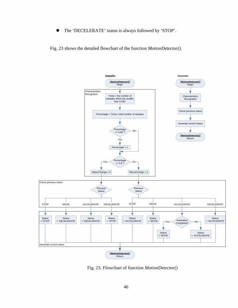
46

The ‘DECELERATE’ status is always followed by ‘STOP’.

Fig. 23 shows the detailed flowchart of the function MotionDetector().

“MotionDetector()”Begin

“MotionDetector()”Return

Temp = the number of samples which are smaller

than 0.05G

Percentage = Temp / total number of samples

Percentage >= 0.85 ?

Percentage = 1

Yes

No

Percentage >= 0.9 ?

StatusChange = 0

Yes No

StatusChange = 1

Previous Status

Previous Status

‘MOVE’

Status = ‘STOP’

Status = ‘DECELERATE’

Status = ‘DECELERATE’

Status = ‘STOP’

‘STOP’ ‘ACCELERATE’ ‘DECELERATE’ ‘MOVE’

Status = ‘ACCELERATE’

Status = ‘MOVE’

‘STOP’ ‘ACCELERATE’ ‘DECELERATE’

EstimationCompleted?Yes No

Status = ‘MOVE’

Status = ‘ACCELERATE’

Status = ‘ACCELERATE’

“MotionDetector()”Return

“MotionDetector()”Begin

Characteristics Recognition

Check previous status

Generate current status

Details: Overview:

Characteristics Recognition

Check previous status

Generate current status

Fig. 23. Flowchart of function MotionDetector()

47

4.2.2.2 Turning Detector

Fig. 24 shows the Z-axis angular rate data. There are five peaks among these data.

Moreover, the turning detector is designed to distinguish ‘a fast turning’ and ‘a slow

turning’ and the noise peaks can be filtered.

In this algorithm, 20 degree/second is set as a threshold. If there are more than 2

samples larger than this threshold among 20~22 samples, it is a fast turning. If there is

only one sample that is larger than this threshold, the program will check the previous or

50 100 150 200 250 300

-80

-60

-40

-20

0

20

40

60

80

X: 301.4Y: -35.38

Time (sec)

Ang

ular

rat

e (d

egre

e/se

c)

X: 209.7Y: -57.04

X: 277.3Y: -39.04

X: 169.5Y: 63.66

X: 62.41Y: 52.14

Zoom in

Zoom in

60 65 70 75 80 85-15

-10

-5

0

5

10

15 X: 74.3Y: 12.25

g

(g

205 210 215-60

-50

-40

-30

-20

-10

0

X: 211.3Y: -21.52

X: 209.1Y: -57.18

Fig. 24. Z-axis gyroscope data

48

the next sample. If one of them is larger than 10 degree/second, then it is a slow turning.

If both of them are smaller than 10 degree/second, then it is just the noise. (See Fig. 25.)

Fig. 25 and 26 describe the algorithm (overview and detailed) of function

TurningDetector(). Generally speaking, the outputs of this function are five different

turning patterns. It is to make sure that this function is capable of detecting typical

turnings. Based on the signal characteristics, we have fast right turning, slow right turning,

fast left turning, slow left turning, and no turning. Specifically, by counting the number of

“TurningDetector()”Begin

“TurningDetector()”Return

Temp1 = the number of samples which are larger than 20 deg/secTemp2 = the number of samples which are smaller than -20 deg/sec

Overview:

Characteristics Recognitionbased on Temp1 and Temp2

Detection result:TuringRightSlow

Detection result:Turing

LeftSlow

Detection result:Turing

LeftFast

Detection result:No

Turning

Detection result:TuringRightFast

If Temp1 = 1 or Temp2 = 1, then check previous/next sample

Fig. 25. Flowchart of Function TurningDetector()

49

samples which are larger than 20 degree/second (or smaller than -20 degree/second), the

classifications could be made.

“TurningDetector()”Begin

“TurningDetector()”Return

Temp1 = the number of samples which are larger than 20 deg/secTemp2 = the number of samples which are smaller than -20 deg/sec

Temp1, Temp2

Percentage = 1flag = 0

Temp1 > 2 or Temp2 > 2Temp1 = 1

postion of this sample

At the beginning Elsewhere At the end

Percentage = 1flag = 1

Check next sample

>= 10 deg/sec else

Percentage = Temp1 / total number of samples

Check next and last

sample

Percentage = 1flag = 1

Percentage = Temp1 / total number of samples

Either one >= 10 deg/sec else

Percentage = 1flag = 1

Check last sample

>= 10 deg/sec else

Percentage = Temp1 / total number of samples

postion of this sample

At the beginning Elsewhere At the end

Percentage = 1flag = 1

Check next sample

<= -10 deg/sec else

Percentage = Temp2 / total number of samples

Check next and last

sample

Percentage = 1flag = 1

Percentage = Temp2 / total number of samples

Either one <= -10 deg/sec else

Percentage = 1flag = 1

Check last sample

<= -10 deg/sec else

Percentage = Temp2 / total number of samples

Temp2 = 1else

Percentage = max(Temp1, Temp2) / total number of samples

Check Percentage

and flagPercentage = 1 and flag = 0

Fast turningFasTu = 1

Temp1 > Temp2 ?

Percentage = 1 and flag = 1

Temp1 > Temp2 ?Yes

Fast turningFasTu = -1

No

Slow turningSloTu = 1

Yes

Slow turningSloTu = -1

No

FasTu = 0SloTu = 0

else

Details:

Characteristics Recognition

Fig. 26. Flowchart of Function TurningDetector() (details)

50

4.2.2.3 Speed Estimation

Fig. 27 shows the X-axis acceleration data. Conventionally, speed can be obtained

by integrating the acceleration. However, a large amount of cumulative error could result

from the integration, which might become larger than the true value. In Table 2, it can be

seen the ‘short term stability’ for accelerometers is 0.2 mg (1mg = 0.00981m/s2). Even

when the accelerometers are not changing (zero acceleration), there is 0.2 mg output.

Though 0.00981 x 2 = 0.01962 m/s2 is a smaller number, it will become 254.2752 km/h2

0 50 100 150 200 250 300

-1.5

-1

-0.5

0

0.5

Time (sec)

Acc

eler

atio

n (g

) Zoom in

15 20 25-0.1

-0.05

0

0.05

0.1

0.15

0.2

0.25X: 19.78Y: 0.2392

Average value

Accelerate

in one hour (3600 seconds). Eventually, the bias will be larger than the true value. This is

Fig. 27. X-axis acceleration data

51

why inertial measurements are not reliable in the long run.

In order to reduce the integration error, the algorithm calculates the integral of

acceleration ONLY in ‘ACCELERATE’ status. And the following rules are made.

‘ACCELERATE’ status begins when the acceleration data exceed the

previous average acceleration

‘ACCELERATE’ status ends when the acceleration data become smaller than

the previous average acceleration. (See Fig. 27).

All samples within this region are called ‘in the same acceleration process’. As a

result, by discarding other useless data, the bias could be minimized. (See Fig. 27)

Pipette() is a function to capture the IMU data packets in each run. Note that the

Pipette() function obtains only 20~22 IMU packets every loop. The Pipette() function

could be regarded as a ‘sliding window’ (the reason why function Pipette() is created was

described in the second and third paragraph of Chapter 4.1 Design Overview). However,

these samples might not ‘cover’ one acceleration status (the length of one ‘sliding

window’ might be shorter than one acceleration status). As a result, there are six different

situations, which are named as the acceleration sampling scenario 1 ~ 6 in Fig. 28, the

acceleration sampling scenario will be simply addressed as the scenario afterward.

52

The scenario 1 only covers the beginning part of one acceleration process without

the peak. The scenario 2 only covers the beginning part of one acceleration process

including the peak. The scenario 3 covers the entire acceleration process. The scenario 4

does not cover the beginning part of one acceleration process. And covers the ending part

of one acceleration process including the peak. The scenario 5 does not cover the

beginning part of one acceleration process and covers the ending part of one acceleration

process without the peak. The scenario 6 does not cover the beginning and ending part of

one acceleration process and covers a middle section with the peak.

Fig. 28. Acceleration sampling scenario 1-3

0 5 10 15 20 25 30

-0.05

0

0.05

0.1

0.15

0.2

Time (sec)

Acc

eler

atio

n (g

)

22 samples/sceniario

Sceniario 3

Sceniario 6

Sceniario 1

Sceniario 5

Sceniario 4Sceniario 2

53

The key of the function Speed() is putting the correct window into an ‘integrator’

to calculate the speed. The following rules are used to deal with the six different

situations.

If ‘the scenario 1’, then put the current window and the following windows

into the integrator until the acceleration process ends.

If ‘the scenario 2’, then put the current window and the next window into the

integrator.

If ‘the scenario 3’, then put the current window into the integrator only.

If ‘the scenario 4’, then put the current window and the previous window into

the integrator.

If ‘the scenario 5’, then put the current window and the previous windows

into the integrator.

If ‘the scenario 6’, then put the current window, the previous windows and

the following windows into the integrator until the acceleration process ends.

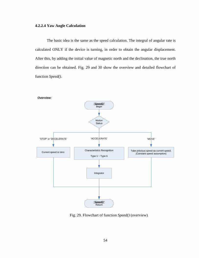
54

4.2.2.4 Yaw Angle Calculation

The basic idea is the same as the speed calculation. The integral of angular rate is

calculated ONLY if the device is turning, in order to obtain the angular displacement.

After this, by adding the initial value of magnetic north and the declination, the true north

direction can be obtained. Fig. 29 and 30 show the overview and detailed flowchart of

function Speed().

“Speed()”Begin

“Speed()”Return

Motion Status

Current speed is zero.

‘STOP’ or 'DECELERATE'

Take previous speed as current speed. (Constant speed assumption)

‘MOVE’

Integrator

Characteristics Recognition

Type 1 ~ Type 6

'ACCELERATE'

Overview:

Fig. 29. Flowchart of function Speed() (overview)

55

“Speed()”Begin

“Speed()”Return

Motion Status

IMUSpeed = 0Estimation Complete

EstNC = 0

‘STOP’ or 'DECELERATE' 'ACCELERATE'

IMUSpeed = previous speed (CB)Estimation Complete

EstNC = 0

‘MOVE’

PreviousWaveform

Type

Type 1, 2

Current waveform type = SpeedEst_Classify()

Type 0 Type 6

Speed = Previous Speed (CB) + SpeedEst_Integrator(Type 1, 2)

Reset Type to zeroEstimation complete

EstNC = 0

Current waveform type = SpeedEst_Classify()

Speed = Previous Speed (CB) + SpeedEst_Integrator(Type 6)

Estimation completeEstNC = 0

Reset Type to zero

Current waveform type = SpeedEst_Classify()

CurrentWaveform

Type

Type 1, 2 Type 3, 5 Type 6

Speed = SpeedEst_Integrator(Type 1, 2)

Estimation incompleteEstNC = 1

Previous waveform type = SpeedEst_Classify()

Current Speed = SpeedEst_Integrator(Type 3, 5)

Previous Speed = SpeedEst_Integrator(Previous waveform type)

Previous waveform type

= 1 or 2?

Yes

No

Speed = Current Speed + Previous Speed

Estimation completeEstNC = 0

Reset Type to zero

Previous waveform type = SpeedEst_Classify()

Current Speed = SpeedEst_Integrator(Type 3, 5)

Previous Speed = SpeedEst_Integrator(Previous waveform type)

Speed = Current Speed + Previous Speed

Estimation completeEstNC = 0

Reset Type to zero

Details:

Characteristics Recognition

Integrator

Fig. 30. Flowchart of function Speed() (details)

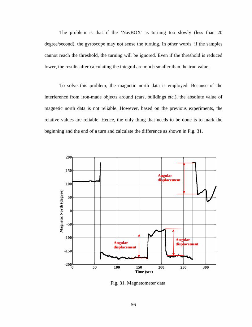
56

The problem is that if the ‘NavBOX’ is turning too slowly (less than 20

degree/second), the gyroscope may not sense the turning. In other words, if the samples

cannot reach the threshold, the turning will be ignored. Even if the threshold is reduced

lower, the results after calculating the integral are much smaller than the true value.

To solve this problem, the magnetic north data is employed. Because of the

interference from iron-made objects around (cars, buildings etc.), the absolute value of

magnetic north data is not reliable. However, based on the previous experiments, the

relative values are reliable. Hence, the only thing that needs to be done is to mark the

beginning and the end of a turn and calculate the difference as shown in Fig. 31.

Fig. 31. Magnetometer data

0 50 100 150 200 250 300-200

-150

-100

-50

0

50

100

150

200

Time (sec)

Mag

netic

Nor

th (d

egre

e)

Angulardisplacement

Angulardisplacement

Angulardisplacement

57

Fig. 32 presents a flowchart outline of function YawCal() and Fig. 33 shows the

detailed flowchart of function YawCal(). The Type 1, …, 6 in the Fig. 32 mean the

acceleration sampling scenario 1, …, 6, respectively. The six different types of the

observed windows mentioned in previous chapters are still applied here. (Refer to Fig. 28

in Chapter 4.2.2.3)

“YawCal()”Begin

“YawCal()”Return

Turning StatusTurning No Turning

Use previous True North Direction as the current value

Prepare for nextCalculation

Overview:

Characteristics Recognition

Type 1 ~ Type 6

Calculate the True North Directionbased on gyroscopes and magnetometers

Fig. 32. Flowchart of Function YawCal() (overview)

58

“YawCal()”Begin

“YawCal()”Return

Turning StatusTurning No Turning

True North Direction (Gyro) = previous valueTrue North Direction (Mag) = previous value

Reset Type to zeroCalculation complete

CalNC = 0

PreviousWaveform

Type

Type 1, 2, 6

Current waveform type = AngDCal_Classify()

Type 0

Current waveform type = AngDCal_Classify()

CurrentWaveform

Type

Type 1, 2 Type 3, 5 Type 6

Previous waveform type = AngDCal_Classify()

Current True North Direction (Gyro) = AngDCal_Integrator()

Current True North Direction (Mag) = AngDCal_Integrator()

PreviousTrue North Direction (Gyro)

= AngDCal_Integrator()

PreviousTrue North Direction (Mag)

= AngDCal_Integrator()

Previous waveform type

= 1 or 2?

Yes

No

True North Direction (Gyro) = Current Value + Previous Value

True North Direction (Mag) = Current Value + Previous Value

Calculation completeCalNC = 0

Reset Type to zero

Previous waveform type = AngDCal_Classify()

True North Direction (Gyro) = Current Value + Previous ValueTrue North Direction (Mag) = Current Value + Previous Value

Estimation incompleteEstNC = 1Type = 6

True North Direction (Gyro) = Previous value (CB) + AngDCal_Integrator()True North Direction (Mag) = Previous value (CB) + AngDCal_Integrator()

Calculation incompleteCalNC = 1

CurrentWaveform

Typeelse

= 6

Calculation completeCalNC = 0

Reset Type to zero

True North Direction (Gyro) = Previous value (CB)

+ AngDCal_Integrator()

True North Direction (Mag) = Previous value (CB)

+ AngDCal_Integrator()

Calculation incompleteCalNC = 1

CurrentTrue North Direction (Gyro)

= Previous value (CB) + AngDCal_Integrator()

CurrentTrue North Direction (Mag)

= Previous value (CB) + AngDCal_Integrator()

PreviousTrue North Direction (Gyro)

= Previous value (CB) + AngDCal_Integrator()

PreviousTrue North Direction (Mag)

= Previous value (CB) + AngDCal_Integrator()

Details:

Characteristics Recognition

Integrator

Prepare for next Calculation

Fig. 33. Flowchart of Function YawCal() (details)

59

4.2.2.5 Inertial Navigation

4.2.2.5.1 Vincenty Formula

The final results of this system will be

longitude and latitude. Based on the previous

discussion, the distance travelled and the bearing

angles are known. Hence, the current problem is

how to calculate the destination point on earth

surface when a start point (lat, long), initial bearing,

and distance are given.

The simplest solution is to use a so-called ‘Haversine Formula’ (See Fig. 34). In

Fig. 34, b is the bearing (brng), d/R is the angular distance (in radians), where d is the

distance travelled and R is the Earth’s radius.

))2sin()1sin()cos(*)1cos()sin()(sin(2tan12

)cos()sin()1cos())cos()1(sin(sin2 1

latlatRdlatRdbrngalonlonbrngRdlat

Rdlatlat

∗−∗∗+=

∗∗+∗= −

(4.2)

However, since Earth is not quite a sphere, there are small errors in using

spherical geometry; Earth is actually roughly ellipsoidal (or more precisely, oblate

spheroidal) with a radius varying between about 6,378km (equatorial) and 6,357km

(polar), and local radius of curvature varying from 6,336km (equatorial meridian) to

Fig. 34. Haversine Formula

60

6,399km (both Poles). This means that errors from assuming spherical geometry might be

up to 0.55% crossing the equator, though generally below 0.3%, depending on latitude

and direction of travel. An accuracy of better than 3m in 1km is acceptable to some

applications, but if greater accuracy is needed, such as in this system, the ‘Vincenty

formula’ should be applied for calculating geodesic distances on ellipsoids, which gives

an accurate results within 1mm.

‘Vincenty formula’ consists of 15 equations and several related rules [26]. Simply

speaking, the ‘Direct Vincenty Formula’ is for deriving the destination point given a start

point, an initial bearing, and a distance travelled. The ‘Inverse Vincenty Formula’ is for

calculating distance between two points on an accurate ellipsoidal model of the Earth.

Direct Vincenty Formula:

),,1,1()2,2( angleheadingdistancelonlatentyDirectVinclonlat = (4.3)

Inverse Vincenty Formula:

)2,2,1,1()( lonlatlonlatcentyInverseVinangleheadingdistance, = (4.4)

61

4.2.2.5.2 Inertial Navigation Using IMU

This function calculates the current position based on IMU data only. It fuses the

Yaw angle (True North Direction) from gyroscopes and magnetometers together by using

the Direct Vincenty Formula mentioned in previous chapters.

Fig. 35 shows the detailed process of the calculation. The current position which

latitude and longitude resulted from last calculation, current velocity, current heading

angle and the sampling interval Δt (time stamp) are known according to Chapter 4.2.2.3

and Chapter 4.2.2.4. So the next position could be calculated easily in accordance with

Eq. (2.1) and the following:

Current Position

True North

Previous Position

Previous Position

Velocity

Heading Angle

Δt

Δt

Next Position

Fig. 35. Dead Reckoning

62

),,,(),( 11 θdLonLatentydirectVincLonLat iiii =++ (4.5)

where Lati+1 is the current latitude position; Loni+1 is the current longitude position; d is

distance; θ is the heading angle.

“IMUNavONLY()”Begin

“IMUNavONLY()”Return

Turning Status

Fast turning No turning Slow turning

Fused Yaw angle = Yaw (by Gyroscopes)

Fused Yaw angle = previous value

(Computation Buffer)

Fused Yaw angle = Yaw (by Magnetometers)

Altitude = GPS Altitude

Roll, Pitch = IMU data

Use Direct Vincenty FormulaInputs: Previous Latitude and Longitude, Fused Yaw angle, Estimated SpeedOutputs: Current Latitude and Longitude

Fig. 36. Flowchart of Function IMUNavONLY()

63

In the Chapter 4.2.2.6 Data Fusion, a loosely-coupled GPS/IMU navigation

system will be discussed, in which the current position, current velocity and current

heading angle could be updated by both GPS and IMU for estimating the next position

with a minimized error. Fig. 36 shows the flowchart of only IMU navigation.

4.2.2.6 IMU Aided GPS Navigation

The key idea is to use IMU as an aid to GPS navigation in order to obtain the best

estimation of current location and orientation. In this discussion, 280 rules have been

designed to deal with different situations. Fig. 37 presents a block diagram of the

organizations of these rules. Note that the final result is a data structure containing the

following fields: Latitude, Longitude, Altitude, Yaw, Pitch and roll (block letters in Fig.

37)

The major function of DataFusion() is to sort each GPS packet into five different

categories:

• Category 1: Use all GPS data (position, heading, and speed)

• Category 2: Use GPS Speed & Heading

• Category 3: Use GPS Heading

• Category 4: Use GPS Speed

• Category 5: Do not use GPS data

As we all know, the GPS receiver provides us different data including position

(latitude & longitude), heading, speed, etc. Depending on the signal quality, sometimes

64

only a few of them can be trusted. For instance, if the current GPS packet is sorted under

“All GPS data are reliable”, that means all the data in this packet can be trusted. And the

position error is small enough. However, if the current GPS packet is sorted under “Only

GPS Speed are reliable”, that means only the speed information from this packet can be

trusted. All the other information including heading and position are not accurate. Fig. 37

only presents a high level block diagram about the organizations of these rules. Fig. 38 ~

39 show the detail of how the five categories are defined. Note that these rules are

obtained based on experiments, experiences, and common senses. Simply speaking, if the

final positioning results are considered as a mixed drink while the GPS data and IMU

data are looked as two different ingredients, our purpose is to find a mixing ratio for the

two ingredients to achieve the best taste. Only here, the “best taste” is the position

accuracy of the final results.

After the categorization, the categorized data will be processed in five different

ways (See Fig. 37). The final data fusion results will include the current position (latitude

and longitude), altitude, yaw, pitch, and roll. In the following text, these results will be

referred to as ‘fused position’, ‘fused heading angle’, and ‘fused speed’

65

In Fig. 37, there are two decision modules marked (1) and (2). Their role is to

categorize all the date into five different categories. The details of module (1) are shown

in Fig. 38. The details of module (2) are shown in Fig. 39.

“DataFusion()”Begin

“DataFusion()”Return

Update current lat/lon using GPS position

Calculate current lat/lon using GPS Heading and

GPS Speed

Calculate current lat/lon using GPS Heading and

IMU Speed

Calculate current lat/lon using GPS Speed and

IMU Heading

Calculate current lat/lon using IMU Heading and

IMU Speed

Altitude = GPS dataYaw = GPS headingPitch = IMU PitchRoll = IMU Roll

Altitude = last GPS dataYaw = GPS headingPitch = IMU Pitch Roll = IMU Roll

Altitude = last GPS dataYaw = GPS headingPitch = IMU Pitch Roll = IMU Roll

Altitude = last GPS dataYaw = IMU headingPitch = IMU Pitch Roll = IMU Roll

Altitude = last GPS dataYaw = IMU headingPitch = IMU Pitch Roll = IMU Roll

Has GPS receiver just experienced

a warm start?(1)

Yes

No

Category 1:Use all GPS data

(position, heading, and speed)

GPS Reliability Check

(2)

Category 2:Use GPS

speed and heading

Category 3:Use GPSheading

Category 4:Use GPS

speed

Category 5:Do not

use GPS data

Fig. 37. Flowchart of Function DataFusion()

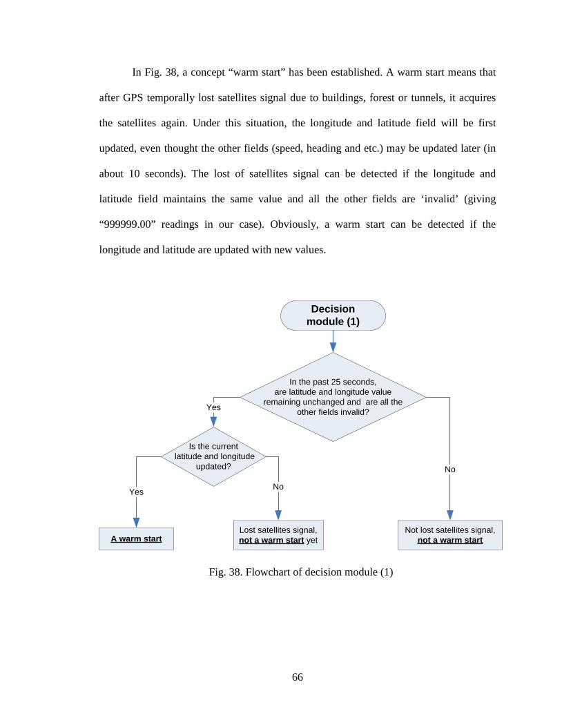
66

In Fig. 38, a concept “warm start” has been established. A warm start means that

after GPS temporally lost satellites signal due to buildings, forest or tunnels, it acquires

the satellites again. Under this situation, the longitude and latitude field will be first

updated, even thought the other fields (speed, heading and etc.) may be updated later (in

about 10 seconds). The lost of satellites signal can be detected if the longitude and

latitude field maintains the same value and all the other fields are ‘invalid’ (giving

“999999.00” readings in our case). Obviously, a warm start can be detected if the

longitude and latitude are updated with new values.

Decisionmodule (1)

In the past 25 seconds, are latitude and longitude value

remaining unchanged and are all the other fields invalid?Yes

No

Is the current latitude and longitude

updated?

Yes No

A warm startLost satellites signal, not a warm start yet

Not lost satellites signal, not a warm start

Fig. 38. Flowchart of decision module (1)

67

heading ≠ 999999 and

speed ≠ 999999?

Yes No

Decisionmodule (2)

Flag1 = 1?

Yes

No

speed = 0?Yes No

Category 1:Use all GPS data

Category 4:Use GPS speed

Yes

Flag2 = 1?Yes

speed = 0?

Yes

No

Category 3:Use GPS heading

Category 2:Use GPS speed

and heading

No

Does accelerometer detect movement?

andcurrent GPS speed – previous

fused speed > 4?Yes

No

Category 5:Do not use GPS data

Category 3:Use GPS heading

No

currentGPS heading – previous fused

heading > 20°?

Flag3 = 1?

Category 4:Use GPS speed

Category 2:Use GPS speed

and heading

Yes

No

heading = 999999 and

speed ≠ 999999?

Category 4:Use GPS speed

YesNo

heading ≠ 999999 and

speed = 999999?

Flag1 = 1?

Yes

Category 5:Do not use GPS data

Yes No

Flag3 = 1?Yes

Flag2 = 1?Yes No

Category 4:Use GPS speed

Category 5:Do not use GPS data

No

Category 3:Use GPS heading

No

Fix Type = 2 or 3?

Yes

Yes

Yes

Number of Satellites in use

>= 3?

Signal Quality Indicator = 1?

Yes

Mode = Automatic?

Status indicator = Valid position?

Yes No

Category 5:Do not use GPS data

Category 1:Use all GPS data

Sub-module (2.1)Set value for Flag1, Flag2, and Flag3

They can be set to ‘0’ or ‘1’

Fig. 39. Flowchart of decision module (2)

68

In Fig. 39, there is a sub-module marked (2.1). Its role is to set three flag values

(Flag1, Flag2, and Flag3) which will be used later. Fig. 40 shows the details of sub-

module (2.1).

Sub-module (2.1)

Is there a turning detected by IMU now

?

Yes No

IMU heading - GPS heading < 13.9°

?Yes No

Flag1 = 1 Flag1 = 0

Flag2 = 1Number of

Satellites in use >= 8?

Yes No

Flag2 = 0Flag1 = 0and

Current GPS heading – previous fused heading

> 20°?

Yes

Flag2 = 0

No

Flag2 = 1

Yes No

Flag3 = 0 Flag3 = 1

No turnings detected by IMU in

the past 20 sec?

Fig. 40. Flowchart of sub-module (2.1)

69

For each of the five Categories, the program has different routines to process the

data. (See Fig. 37). In this way, the GPS data and IMU data are fused together to produce

more robust navigation and orientation.

For Category 1 “Use all GPS data”, IMU data will not be used for positioning

since the accuracy of GPS data is acceptable.

For Category 2 “Use GPS Speed & Heading”, the current position will be

calculated based on GPS Speed and Heading using Vincenty Formula [26].

For Category 3 “Use GPS Heading”, the current position will be calculated based

on GPS Heading and IMU Speed information.

For Category 4 “Use GPS Speed”, the current position will be calculated based on

GPS Speed and IMU Heading information.

For Category 5 “Do not use GPS data”, the current position will be calculated

based on IMU Speed and IMU Heading information.

70

4.3 Evaluation Method for Data Fusion Results

The Final Stage is for comparing and results evaluation. The results from function

DistCal() could show the differences among IMU Distance, Laser Speedometer Distance,

GPS Distance and True Distance. The function QualityInspector() evaluates the data

fusion results to see how well the GPS data and Fused data fit the true trace (see Fig. 41).

The detailed algorithm of QualityInspector() will be discussed in the following Chapters.

Begin

Distance Calculation“DistCal()”

Evaluates the data fusion results“QualityInspector()”

Plot the results“PlotPos()”

End

Input:Estimated SpeedLaser Speedometer dataGPS SpeedIMU timestampTrueTrace

Output:IMU DistanceLaser Speedometer DistanceGPS DistanceTrue Distance

Input:GPS dataFused IMU dataFused GPS+IMU dataTrue Trace

Output:GPS QualityIMU Quality Data Fusion Quality(In the form of coefficient of determination R-squared)

Input:GPS dataFused IMU dataFused GPS+IMU dataTrue Trace

Output:True TraceGPS TraceFused IMU TraceFused GPS + IMU Tracein the same figure

Fig. 41. Flowchart of the Final Stage

71

A laser speedometer is installed on the rolling cart. This device could give some

accurate speed information which will be used to generate a true trace. Once the true

trace (black dot-line in Fig. 42) is obtained, the distance between GPS raw data and the

true trace is the error (grey lines which connect GPS data with true trace in Fig. 44). The

average error could be calculated by adding all errors together and divided by the total

number of samples. Fig. 45 illustrates distance between true trace and inertial navigation

results and Fig. 46 displays distance between true trace and fused data.

In Fig. 42, 43, and 44, the length of the gray lines between the blue dots (position

data from GPS receiver) and the black line are the positioning error.

Fig. 42. Distance between true trace and GPS raw data

-75.1533 -75.153 -75.1528

39.9826

39.9827

39.9829

Longitude (degree)

Lat

itude

(deg

ree)

Error = 10.3471 m (GPS)

True TraceGPSIMUFused

72

Fig. 43. Distance between true trace and inertial navigation results

Fig. 44. Distance between true trace and fused data

-75.1533 -75.153 -75.1528

39.9826

39.9827

39.9829

Longitude (degree)

Lat

itude

(deg

ree)

Error = 11.5705 m (IMU)

True TraceGPSIMUFused

-75.1533 -75.153 -75.1528

39.9826

39.9827

39.9829

Longitude (degree)

Lat

itude

(deg

ree)

Error = 2.662 m (Fused)

True TraceGPSIMUFused

73

CHAPTER 5

EXPERIMENTS AND RESULTS

5.1 Experiment Conditions

A prototype of the novel system with the GPS and the IMU integration based on

the rule-based data fusion algorithm, namely NavBOX, has been built. And a series of

field experiments with NavBOX have been conducted to evaluate the position error.

• Route shape

Fig. 45. Route Type 029

74

We designed four different routes as in Fig. 45~48.

The “stressed environments1

” is the area between the 9-floor building (55 m high)

and the 3-floor building (15m high), and the area beneath the 9-floor building.

Route 029, 030, and 032 are used in our outdoor experiments. Also, we have

designed outdoor/indoor mixed experiments. As shown in Fig 45.

The rolling cart (Fig. 15 in Chapter 3.2) was moved inside the building and

moved out a few minutes later.

1 The stressed environments are defined as the places beneath the buildings, inside the tunnels, forests, and indoors.

Fig. 46. Route Type 030

75

Fig. 47. Route Type 032

Fig. 48. Route Type 037

76

Table 9. A part of experimental trajectories

Name1 Route 029 Route 030 Route 032 Route 037 Trajectory

Route length (m) 390.34 413.12 347.70 425.90

Number of repeated trials

13 7 7 13

Outdoor/indoor Outdoor Outdoor Outdoor Partial indoor2 Environment Partially stressed

environment3Exposed area

Partially stressed

environmentPartially stressed

environment 3

5.2 Devices

• NavBOX (GPS, IMU, Laser Speedometer)

• Rolling cart

• Stopwatch

1 Route 31 and Route 33~36 are other designed routes that we did not use. They are similar to route 032 and 037. 2 The mobile cart was first moved through the area between the 9-floor building (height of 55 m) and the 3-floor building (height of 15 m), then entered the area beneath the 9-floor building and moved out a few minutes later (see the shadow part, the route 037 in Table 1). 3 The stressed environment (see the shadow parts, the routes 029 and 032 in Table 1) is the area between the 9-floor building (height of 55 m) and the 3-floor building (height of 15 m).

77

5.3 Experiment Result Discussion

Each test started with a starting point, moved along each route and ended at the

specified destination. The measured instantaneous position (latitude/longitude) can be

obtained based on the NavBOX, which can be used to compare with the true position

(latitude/longitude) to determine the absolute position error. The average position error

can hence be acquired using the instantaneous absolute position errors in each run. The

test mentioned above was repeated several times under an identical operating condition to

examine the position accuracy and the repeatability. The bar chart of the average position

error for routes 029, 030, 032 and 037 is shown in Fig. 49. The experimental results show

that: (1) in each route, the mean of the average position error from the IMU data-only is

always the highest, the mean of the average position error from the GPS data-only is in

the middle, the mean of the average position error from the GPS/IMU fused system is the

lowest. This may suggest that the GPS/IMU fused system improves the navigation

performance and eliminates the error; (2) for routes 030, 032 and 037, the means of the

average position errors from the three different combinations display a rise due to

increase of the extent of the stressed environment, in turn, exposed area (route 030),

partially stressed environment (route 032) and partial indoor and stressed environment

(route 037). And the mean of the average position error from the GPS data-only in the

route 029 is similar to the route 032 but the mean of the error from the GPS/IMU fused

system in the former is slightly greater than the latter. It seems to be that the GPS signals

might be weakened or even disappear in urban canyons and indoors. However, the

GPS/IMU fused system will augment GPS signals and obtain the better position accuracy

than the GPS signal-only. (3) the mean of the average position error for the GPS/IMU

78

fused system is relatively lower in routes 030 and 032, the highest in the route 037, which

further implies the limitation and the constrain of the GPS signals-only in stressed

environments, also the improvement from the GPS/IMU fused system.

Fig. 49. Bar chart of average position error for the route 029, 030, 032 and 037

GPS,

6.7

897

GPS,

2.7

285

GPS,

6.6

833

GPS,

14.

4436

IMU

, 28.

3596

IMU

, 15.

1417

IMU

, 19.

8207 IM

U, 3

1.22

43

Fuse

d, 2

.207

2

Fuse

d, 1

.431

6

Fuse

d, 1

.389

7

Fuse

d, 2

.747

3

0

10

20

30

40

50

60

70

Route 029 13 Trials

Route 030 7 Trials

Route 032 7 Trials

Route 037 13 Trials

Aver

age

Posi

tion

Erro

r (m

)

Trial Route

GPS Data Average Error

IMU Data Average Error

Fused Data Average Error

79

Table 10. Experiment statistics

Route Repeat

Average GPS data

Error (m)

Average IMU data

Error (m)

Average Fused data

Error (m)

Fused data Relative

improvement comparing to

GPS

Fused data Relative

improvement comparing to

IMU

Comments

029 13 6.7897 28.3596 2.2072 67.49% 92.22% Outdoor 030 7 2.7285 15.1417 1.4316 47.53% 90.55% Outdoor 032 7 6.6833 19.8207 1.3897 79.21% 92.99% Outdoor

037 13 14.4436 31.2243 2.7473 80.98% 91.20% Out/Indoor mix

Fig. 49 is the organized bar chart interpreting Table 10. There are four different

routes (route 029, 030, 032, and 037), for each type of route, numbers of trials were

repeated (see Table 9). The average errors of each route have been calculated and shown

in the bar chart. One trial was picked from each route and shown below.

80

• Route 029

This plot was generated by Matlab; see Fig. 45 for Google Earth image. We

repeated the experiments thirteen times on route 029. Fig 50 is the results of one of the

thirteen trials, STD means standard deviation. Fused data error is always smaller than

GPS only or IMU only error.

Fig. 50. Data fusion positioning results (Route 029)

-75.154 -75.1535 -75.153 -75.1525 -75.152 -75.1515

39.982

39.9825

39.983

39.9835

39.984

32.146 m

2-floor Apartment

9-floor Engineering Building

Longitude (degree)

Parking Lot No. 10

3-floor Tyler Art School

3-floor Dept. of Life Science

Error = 11.5705 m (IMU)Error = 2.662 m (Fused)

Error = 10.3471 m (GPS)

Lat

itude

(deg

ree)

True TraceGPSIMUFused

81

• Route 030

This plot was generated by Matlab; see Fig 46 for Google Earth image. This route

is actually a rectangular around parking lot 10.

We repeated the experiments seven times on route 030. Fig. 51 is the results of

one of the seven trials. Note that the GPS error is very similar to fused data error. That is

because route 030 is not in a stressed environments, GPS signal is not blocked by any

buildings. Even so, the fused data error is still smaller than GPS error.

Fig. 51. Data fusion positioning results (Route 030)

-75.1535 -75.153 -75.1525 -75.152

39.9826

39.9828

39.983

39.9832

39.9834

39.9836

39.9838

39.984

39.9842

2-floor Apartment

22.381 m

Parking Lot No. 10

Longitude (degree)

3-floor Tyler Art School

Error = 3.0197 m (GPS)Error = 10.7514 m (IMU)Error = 1.2251 m (Fused)

Lat

itude

(deg

ree)

True TraceGPSIMUFused

82

• Route 032

This plot was generated by Matlab; see Fig. 47 for Google Earth image. Route

032 is similar to Route 029. We repeated the experiments seven times on route 032. Fig.

52 is the results of one of the seven trials.

Fig. 52. Data fusion positioning results (Route 032)

-75.1545 -75.154 -75.1535 -75.153 -75.1525 -75.152 -75.1515

39.982

39.9825

39.983

39.9835

39.984

33.183 m

2-floor Apartment

9-floor Engineering Building

Parking Lot No. 10

Longitude (degree)

3-floor Tyler Art School

3-floor Dept. of Life Science

Error = 1.566 m (Fused)

Error = 5.4351 m (GPS)Error = 18.3458 m (IMU)

Lat

itude

(deg

ree)

True TraceGPSIMUFused

83

• Route 037

This plot was generated by Matlab; see Fig. 48 for Google Earth image. Some

parts of Route 037 are inside a building where GPS is not working. We repeated the

experiments thirteen times on route 037. Fig. 53 is the results of one of the thirteen trials.

When there is no GPS signal, the data fusion algorithm can still track the device by using

other sensors. In the end, the accuracy is better than GPS.

Fig. 53. Data fusion positioning results (Route 037)

-75.154 -75.1535 -75.153 -75.1525 -75.152 -75.1515 -75.151

39.982

39.9825

39.983

39.9835

39.984

32.974 m

2-floor Apartment

9-floor Engineering Building

Longitude (degree)

Parking Lot No. 10

3-floor Tyler Art School

3-floor Dept. of Life Science

Error = 8.1267 m (GPS)Error = 43.0206 m (IMU)Error = 1.4788 m (Fused)

Lat

itude

(deg

ree)

True TraceGPSIMUFused

84

5.4 Indoor Experiments

Besides all those outdoor and partial indoor experiments, a series of indoor

experiments has also been designed. These experiments have been carried out in the hall

way of engineering building, 7th floor (See Fig. 54). Fig. 54 is actual the floor plan of 7th

In addition, a Laser Alignment Technique has been designed. A laser alignment

station was installed beside the experiment route. It generates two parallel laser beams

floor, engineering building at Temple University. The experiments were started at the end

of the hallway, and circled around the aisle for four times, ended at the point labeled

‘End’.

Fig. 54. Route Type 040

85

across the experiments route. Whenever the rolling cart passes the laser beams, the

orientation and position will be reset to true value (See Fig. 55). Considering the walking

speed, the resetting happens every 40 seconds.

In Fig. 55, the red rectangle is the laser beam. Based on the linearity of laser, it

can be used to reset the orientation.

Seven trials have been carried out based on Route Type 040. The experiments

results are shown in a bar chart (See Fig. 56). The bars show the average position errors

in meter. The error bars show the maximum and minimum value in seven trials.

Side View

X, roll axis Z, yaw axis

Top View

Y, pitch axis

Fig. 55. Laser Alignment

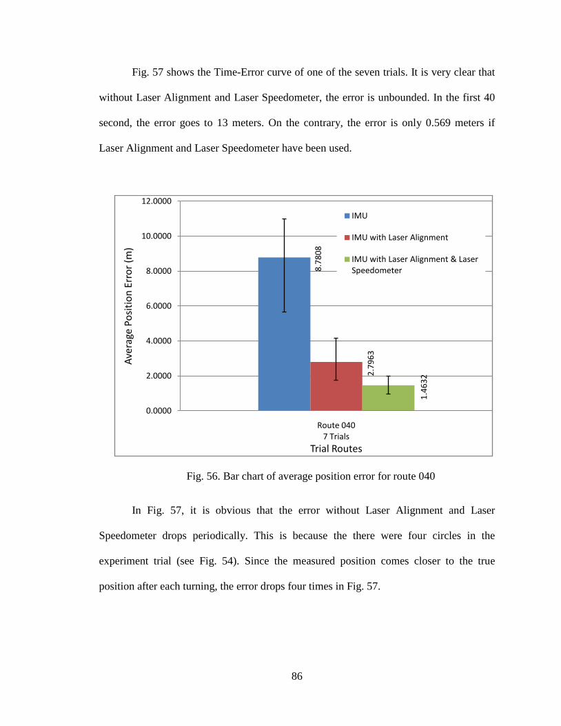
86

Fig. 57 shows the Time-Error curve of one of the seven trials. It is very clear that

without Laser Alignment and Laser Speedometer, the error is unbounded. In the first 40

second, the error goes to 13 meters. On the contrary, the error is only 0.569 meters if

Laser Alignment and Laser Speedometer have been used.

In Fig. 57, it is obvious that the error without Laser Alignment and Laser

Speedometer drops periodically. This is because the there were four circles in the

experiment trial (see Fig. 54). Since the measured position comes closer to the true

position after each turning, the error drops four times in Fig. 57.

Fig. 56. Bar chart of average position error for route 040

8.78

08

2.79

63

1.46

320.0000

2.0000

4.0000

6.0000

8.0000

10.0000

12.0000

Route 0407 Trials

Aver

age

Posit

ion

Erro

r (m

)

Trial Routes

IMU

IMU with Laser Alignment

IMU with Laser Alignment & Laser Speedometer

87

Also, there is an increasing trend in the error with Laser Alignment and Laser

Speedometer in Fig. 57. But this is just a single case. The errors after each resetting are

random due to speed and heading estimation.

In each of these experiments, the rolling cart will pass cross the laser beam four

times. Whenever this happens, the orientation and position will be reset to true values. In

Fig. 57, the position error goes to zero if the rolling cart is aligned with two parallel laser

beams.

Fig. 57. IMU Time-Error Curve of Route 040

0 20 40 60 80 100 120 140 160 180 2000

2

4

6

8

10

12

14

16

18

20

22

X: 40Y: 13

Time (sec)

Err

or (m

)

X: 40Y: 0.569

X: 50Y: 14.28

X: 50Y: 1.894

X: 76Y: 15.07

X: 76Y: 1.98

X: 112Y: 16.4

X: 112Y: 3.655

X: 155Y: 18.34

X: 155Y: 3.784

X: 208Y: 19.85

X: 208Y: 1.877

IMU Time-Error with Laser Alignment & Laser SpeedometerIMU Time-Error without Laser Alignment & Laser Speedometer

88

CHAPTER 6

INTEGRATED SYSTEM DESIGN

6.1 Backgrounds

The NavBOX was designed for testing purpose only. It was assembled from off-

the-shelf modules and products (See Chapter 3, Fig. 13, and Fig. 14). So we could

temporarily ignore the detailed structure inside each module and focus on the top-level

system design. This is important during the initial stages in this project. The NavBOX

design procedures has to be simplified, otherwise the system complexity is overwhelming.

However, after a series of field experiments, the NavBOX design was proved to be

inadequate for future development. The main reasons are:

• The data acquisition and process algorithm inside the IMU was unknown.

• The data fusion can only be done after the experiments (not real-time/on-board).

• It is difficult to add new sensors to the system.

• The entire system (NavBOX) is too large and too complicated for operation.

As a result, an advanced system was designed, the system requirements are:

• All levels of the system should be transparent1

• The data fusion should be real-time processing and done on board.

to us.

1 The hardware connections, the firmware program, and the user interface program should be designed by us instead of using off-the-shelf products or modules.

89

• It should be easy to add other sensors or accessories.

• The size of the system should be minimized.

Based on these requirements, a new system was designed. We name it ‘NavBOARD’.

6.2 Top-level Design

There are two methods for assembling this navigation system. One is single

microprocessor mode, which is to utilize only one microprocessor to interface with all the

sensors, modules, and complete the data fusion. Another is dual microprocessor mode,

which is to use one microprocessor to interface with only inertial sensors and use another

microprocessor to complete the data fusion. Considering that we have seven inertial

sensors, a GPS receiver, a RF module, a Personal Digital Assistant (PDA), and a LCD

module. If we use only one microprocessor, there are not enough resource for all the

sensors and modules. Moreover, the workload for one microprocessor is too heavy. The

complexity of its firmware is also extremely high. In conclusion, we prefer to use the

dual microprocessor mode (see Fig. 58).

Microprocessor I will be used to interface with all the inertial sensors. It receives

all the raw data from the sensors. Then the raw data will be calibrated, time stamped, and

converted to binary code for transmission to Microprocessor II.

Microprocessor II can be called our “data fusion processor”, since it gathers and

processes data from GPS module (GPS receiver) and Microprocessor I. Moreover, after

the data fusion, it can transmit the data to a RF module, a PDA, and a LCD display.

90

These modules are optional for different situation. The RF module is for wireless type of

usage or sensor network. The PDA is for standalone operation. The LCD display is for

basic tests and debugging.

91

Printed Circuit Board

Inertial Measurement Unit

Triaxial Magnetometer

Temperature Sensor

GPS Module

Antenna

Microprocessor I(Acquire and process inertial sensors data)

RAM

Pressure Sensor

16-bit A/D

Convertor

Multiplexer

ROM

EEPROM

I/O Ports

DataControl signal

Data Fusion &Transmission Unit

Microprocessor II(Fuse GPS and inertial navigation data)

RAM

ROM

EEPROM

I/O Ports

GPS ModuleSocket

LCD ModuleSocket

PDASocket

RF Module

PDA LCDModule

I/O Ports

I/O Ports

Legend:

Dual axis Accel

Triaxial Accelerometer

Single axis Gyro

Triaxial GyroscopeSingle axis Gyro

Single axis Gyro

Dual axis Accel

Fig. 58. Top-level System Diagram

92

6.3 Bill of Materials

Table 9 shows the critical information such as model, power consumption, and

cost of all the major components we have used in our design.

Table 11. Bill of Materials

Component Model Power Consumption Quantity Unit Cost

Microprocessor I & II RCM 3100 75 mA @ 3.3 V 2 $ 62.50 Triaxial Magnetometer HMC1053 10 mA @ 5.0 V 1 $ 55.00

Dual Axis Accelerometer ADXL210E 0.6 mA @ 5.0 V 2 $ 17.46 Single Axis Gyroscope ADXRS610 3.5 mA @ 5.0 V 3 $ 49.50 Temperature Sensor

Pressure Sensor MPXAZ4100A 7.0 mA @ 5.0 V 1 $ 15.09 Multiplexer MAX4617CUE 10 µA @ 5.0 V 2 $ 2.70

A/D Convertor LTC1864 0.85 mA @ 5.0 V 1 $ 15.00 D/A Convertor LTC1665 0.45 mA @ 5.0 V 1 $ 6.38 GPS Module GPS15L 85 mA @ 5.0 V 1 $ 55.50 RF Module AC4490-200M 68 mA @ 5.0 V 1 $ 62.50

LCD Module LCD/Keypad 170 mA @ 5.0 V 1 $ 79.00 PDA1 Dell Axim x51v 220 mA @ 3.7 V 1 $ 400.00 Total N/A 503.02 mA @ 5.0 V N/A $ 602.29

We chose RCM 3100 as our powerful microprocessor module to control all the

sensors. The new RCM 3100 is a high-performance, low-EMI microprocessor module

designed specifically for embedded control, communications, and Ethernet connectivity.

The 8-bit RCM 3100 outperforms most 16–bit processors without losing the efficiency of

an 8–bit architecture. Extensive integrated features and glue less architecture facilitate

rapid hardware design, while a C-friendly instruction set promotes efficient development

of even the most complex applications.

1 PDA is an independent device that is not included in the calculation of total power consumption and total cost.

93

In addition, the RCM 3100 is fast, running at up to 55.5 MHz, with compact code

and direct software support for 1 MB of code/data space. Typically operating at 3.3 V

(with 5 V tolerant I/O), the RCM 3100 boasts 6 serial ports with IrDA, 56+ digital I/O,

quadrature decoder, PWM outputs, and pulse capture and measurement capabilities (see

Fig. 59). It also features a battery-backable real-time clock, glue less memory and I/O

interfacing, and ultra-low power modes. 4 levels of interrupt priority allow fast response

to real-time events. Its compact instruction set and high clock speeds give the RCM 3100

exceptionally fast math, logic, and I/O performance.

1 Note that RCM 3100 is not a microprocessor chip but a miniature PCB board on which the Rabbit 3000 microprocessor and other peripheral circuit are integrated.

PB1,PC7, /RESPC6

PG2, PG6PG3, PG7

PC1, PC3, PC5PC0, PC2, PC4

/RESET,/IOWR,

STATUSSMODE0SMODE1

PG0-PG1,PG4-PG5

PB0,PB2-PB7 PD0-PD7

PF0-PF7

PE0-PE1,PE3-PE7

PA0-PA7

Port B

RABBIT 3000 Port F

Port E

Port D

Port G(+Serial Ports)

Misc. I/O

Port A

Port C(Serial Ports B, C & D)

Port G(Serial Ports E & F)

ProgrammingPort

(Serial Port A)

Real-Time Clock

Watchdog

11 Timers

Slave Port

Clock Doubler

RAM Buckup BatterySupport Flash

Fig. 59. Ports of RCM 31001

94

6.4 The PCB Layout Design

The gyroscope ADXRS610 is for a single axis. The accelerometer ADXL210 has

dual axles. In order to measure three axis angular rates and three axis acceleration, we

have to install them perpendicularly to each other. (See Fig. 60)

As a result, we designed two PCB boards. One is “Peripheral Board” for

gyroscopes and accelerometers; another “Main Board” is for all other components. They

will be installed (solder) perpendicularly to each other. (See Fig. 61, there are two same

peripheral boards for four sensors.)

Accel #1 and Gyro #1 will be on one peripheral board. Accel #2 and Gyro #3 will

be on another peripheral board. Gyro #2 and other components will be on the main board.

(See Fig. 57)

Gyro #1

Gyro #2

Gyro #3

XZ

YAccel #1 Accel #2

Y X

Z Z

Fig. 60. Installation of gyroscopes and accelerometers

95

This configuration could enable all 3 axes measurements of accelerations and

angular rates which gives our system 6 DOF1

General ideas were shown in Fig. 60 and Fig. 61. For designing these boards, we

have used Altium Designer 6 as PCB layout design tool. Fig. 62 shows the top level

schematic. There are totally 14 modules in the design.

.

1 DOF: Degrees of Freedom

Main Board

Peripheral Board #1 Peripheral Board #2

Gyro #2

Accel #1

Gyro #1

Accel #2

Gyro #3

Fig. 61. Installation of Peripheral Boards and Main Board

96

The PCB layout design is right after the schematic plotting1

1 The detailed circuit design of each module is not included in this thesis.

. See Fig. 63 ~ 68, all

the components were fit into a 3.2 x 3.45 inch main board and two 0.78 x 0.545 inch

peripheral boards. The main board is a 6-layer board. The peripheral board has 3 layers.

Fig. 63 and Fig. 64 are the sketch block diagrams without many details. Fig. 65 ~

Fig. 68 are the detailed PCB layouts (Altium Designer 6).

MagnetometerModule

Peripheral BoardsConnectors

GyroscopeModule

Pressure SensorModule

Signal ConditionModule Microprocessor I Microprocessor II

GPS ModuleConnector

RF Module

LCD ModuleConnector

ExtensionConnector

Fig. 62. Top-level Schematic (The arrows indicate the interaction (data/control) between components)

97

PCB Layout Main Board (Top view)

Power UnitRF Module

Microprocessor #1 LCDSocket

LCDDrive Circuit

Indicator LED #1Indicator LED #2Indicator LED #3

Indicator LED #3

&Indicator LED #4

Indicator LED #5Indicator LED #6

RF Antenna

PCB Layout Peripheral Board (Top view)

Accelerometer

Fig. 63. Main board layouts (Top view) PCB Layout Main Board (Bottom view)

Power Unit

TriaxisMagneto-

meter

Microprocessor #2

Pressure sensor

Peripheral Board #1(Gyroscope #1

Accelerometer #1)

Gyroscope #3

Peripheral Board #2

(Gyroscope #2

Accelerom

eter #2)

BackupBattery

SignalCondition

Module

PCB Layout Peripheral Board (Bottom view)

Gyroscope

Fig. 64. Main board layouts (Top view)

Connect to PCB Board No. 1

Connect to PCB Board No. 1

98

Fig. 65. Main board layouts (Top view)

Fig. 66. Peripheral board layouts (Top view)

Fig. 67. Peripheral board layouts (Bottom view)

Fig. 68. Main board layouts (Bottom view)

Connect to PCB Board No. 1

Connect to PCB Board No. 1

Connect to PCB Board No. 1

99

6.5 The Prototype and Conclusions

For this Navigation system, a powerful microprocessor is an essential part. This is

because there are seven sensors data to be processed by real-time operation. If we

configure seven 16-bit A/D converters for each sensor, there will be a waste of resources.

Moreover, the microprocessor’s serial/parallel ports turn out to be not enough in this

configuration. As a result, the idea is that three sensors share one A/D converter.

Considering the high speed of the microprocessor and A/D converters, it will not affect

Fig. 69. NavBOARD prototype comparing with NavBOX

100

the performance of the system. Though this configuration may bring some trouble in

layout, it optimizes the system.

All the data will be transferred to a desktop/laptop computer wirelessly. A Matlab

program was designed to collect and process the data in real time. (See Appendix C:

Graphic User Interface.)

101

CHAPTER 7

PERSONAL NAVIGATION SYSTEM

7.1 Introduction

Positioning and navigation for airplanes, automobiles, and pedestrians are critical

function today. For outdoor operations, several techniques are extensively used currently,

such as GPS and cellular-based methods. For indoor operations, there is RF based

positioning technique, the so-called “RFID”. However, there are some other important

indoor scenarios that cannot be fulfilled by this kind of techniques, such as the building

floor plan is unknown, bad RF transmission due to fire, smoke, and humidity conditions,

no RF infrastructure, etc. In order to adjust to these conditions, new techniques need to be

developed.

The methods proposed here are MEMS1

1 MEMS: Micro-electro-mechanical systems is the technology of the very small, and merges at the nano-scale into nano-electro-mechanical systems (NEMS) and nanotechnology

inertial sensors based. Simply speaking,

one or more micro scale MEMs inertial sensors such as accelerometer, gyroscopes, and

magnetometers are attached onto human body. These sensors could measure multiple

parameters including acceleration, angular rate, and earth magnetic field strength

(magnetic north). Based on these data, some algorithms have been design and developed

to calculate or estimate the position of a walking (running) person.

102

In our study, three cases have been

introduced. Since there are different motions

characteristics on different parts of human

body, the inertial sensors are attached to three

different parts of human body in these three

cases, they are waist, knee and foot.

In each of these cases, data has been

collected on a walking person, algorithms have

been developed. Along with the results, these cases are discussed in the following

chapters in detail.

7.2 Method #1 Waist Attached Sensor

7.2.1 Step Counter

While walking, the knee is bent only when the foot is off the ground. Therefore

we can look at the leg as being a lever of fixed length while the foot is on the ground.

Since the hip and, by extension, the upper body moves vertically when walking, we can

measure the vertical acceleration by attaching an acceleration sensor to the hip of a

person. (See Fig. 70)

1 An accelerometer.

Fig. 70. A walking person with an

inertial sensor1 attached on the waist

103

The frequency of leg movement while walking is about 2~3 Hz, so we chose the

sampling rate to be 20 Hz. Fig. 72 shows a data segment we recorded from a walking

person.

Acceleration was processed with a low-pass filter (FIR type-1, 24-orders, cut-off

frequency 2 Hz), which will remove undesirable noise (frequency > 2 Hz).

By counting the positive (or negative) peaks of the above waveform we can

determine how many steps a person has walked. In addition, we also could count how

many times the waveform crosses zero. To determine the number of steps, we implement

this zero crossing counter in a Matlab program.

HIP

RIGHTLEG

LEFTLEG

RIGHTLEG

LEFTLEG

HIP HIP

Amax1

Amin1 Amin2

Stride1 Stride2

RIGHTLEG

LEFTLEG

HIPHIP

Amax2

Fig. 71. Vertical movement of hip while walking

104

7.2.2 Stride Length Calculation

Simply speaking, we are trying to find the relation between Amax - Amin and the

stride length (i.e., to find a function of stride length = f (Amax - Amin)). Fig. 72 shows the

vertical movement of hip while walking. Note that there are large differences between

original signal and filtered signal. This is because there exists vibration noises. Even

though the FIR1 filter has attenuate the original signal, it will not affect our final results

since the coefficients could be used to compensate the attenuation. During the time of

Stride 1, we observe a positive peak (Amax1) and a negative peak (Amin1) in the z-axis

acceleration waveform. (See Fig. 72) The same thing happens during Stride 2. Basically,

if the stride length is getting longer, the Amax - Amin will be larger. So if we find the

relation stride length = f (Amax - Amin

), the stride length could be calculated. Using the

Fig. 72. Vertical acceleration during walking

5 6

-0.5

-0.4

-0.3

-0.2

-0.1

0

0.1

0.2

0.3

0.4

0.5

Time (sec)

Z-a

xis a

ccel

erat

ion

(G)

Original SignalProcessed by FIR1 Filter

105

method from “7.2.1 Step Counter”, we could identify the beginning and the end of one

stride. Then we just need to find the Amax and Amin within one stride and simply do a

subtraction. Repeating this action, we could record the Amax - Amin for each stride. Next

step is to get enough data to generate an average Amax - Amin

Table 12. Empirical Curve Experiments Data

of one particular stride

length.

To this end, a series of experiments were carried out. We chose 9 different stride

length, they were 1, 1.25, 1.5, 1.75, 2, 2.25, 2.5, 2.75, 3 ft, i.e., A person walked using

these 9 different step length and recorded the vertical acceleration (Z-axis) data (See Fig.

68). We repeated these kinds of experiments total of 135 times. Table 1 is the results

which indicate the average value of Amax - Amin

Average A

for 9 different step lengths. Fig. 69 is the

graph of the data in Table 12.

max - Amin

value (G*

Step length (ft) )

Number of experiments

0.053226 1 18 0.074336 1.25 10 0.101185 1.5 12 0.134529 1.75 10 0.194664 2 32 0.249616 2.25 10 0.323300 2.5 15 0.374858 2.75 13 0.458741 3 15

106

Moreover, we have compared our results (Table 12) with another empirical

formula derived by Harvey Weinberg, an engineer from Analog Device. In his

application [23], Mr. Weinberg

used

4minmax AAStride −≈ (7.1)

to calculate the step length. The

sensor he used was ADXL202,

while ours is ADXL210. Fig. 73

& 74 shows both our data and the

value calculate from equation

(7.1).

Obviously, equation (7.1)

can not satisfy our experiments

data. There exist large errors.

By using polyfit function in

Matlab, we could derive our own

empirical equation. The key is

using a curve fit to match all of the

data sets as closely as possible. Fig.

70 shows the values calculated by

the new equation (7.1) derived by polyfit in Matlab.

Fig. 73. Experiment data of Table 1

Fig. 74. Experiment data & Equation 6.1

0 0.1 0.2 0.3 0.4 0.5 0.60.2

0.3

0.4

0.5

0.6

0.7

0.8

0.9

1

Average Z-axis acceleration peak-peak value (G)

Stri

de L

engt

h (m

)

WeinbergExperiment

0 0.1 0.2 0.3 0.4 0.5 0.60.2

0.3

0.4

0.5

0.6

0.7

0.8

0.9

1

Average Z-axis acceleration peak-peak value (G)

Stri

de L

engt

h (m

)

WeinbergExperimentEquation (6.2)

107

dcxbxaxstride +++≈ 23 (7.2)

Where x is the z-axis acceleration peak-peak value Amax - Amin

[ ]0.42905212.96048229.884192-30.390920

during each stride,

a, b, c and d is the coefficients of this polynomial. They are

Finally, we have established the function mentioned in the beginning of this

chapter:

( ) ( ) ( ) ( ) dAAcAAbAAaAAfstride +−+−+−≈−= minmax2

minmax3

minmaxminmax

[ ] [ ]0.42905212.96048229.884192-30.390920dcba = (7.3)

7.2.3 Distance Calculation

If we use Equation (7.2) from “7.2.2 Stride Length Calculation” in every stride

and then sum all the stride lengths together, we can determine the distance a person has

walked. Let N be the total number of strides and let n indicates each stride, we have

( ) ( ) ( )[ ]∑∑==

−==N

n

N

nnAnAfnstrideDistance

1minmax

1 (7.4)

108

7.2.4 Heading Angle Determination

Since the gyroscope (See Fig. 75) could provide us

the angular rate data, it is easy to get the heading changing

simply by integration (See Fig. 76).

Continuous-time: dtt

t∫=2

1

ωθ (7.5)

Discrete-time:( ) ( ) ( ) ( )[ ]

(7.6)1

15.01

×

++×+=+

sF

kkkk ωωθθ

Where:

θ

ω is the angular rate

(degree/second).

is the heading angle

(degree).

k is the serial number if

samples.

Fs

In the end, instead of knowing the absolute value of heading, we can calculate the

relative heading of initial heading direction.

is the sampling rate.

Fig. 75. Gyroscope

Fig. 76. Z-axis angular rates

27.6 27.8 28 28.2-55

-54

-53

-52

-51

-50

-49

-48

-47

Time (sec)

Z-a

xis a

ngul

ar r

ate

(deg

ree/

sec)

ω (k+1)

ω (k)

1/f

109

7.2.5 Position Tracking

From 7.2.3 Distance calculation, we obtained the length at every stride.

From 7.2.4 Heading angle determination, we obtained the heading information.

In this part, we will combine the above two parameters in order to calculate a

person’s position in terms of (x, y) on a xOy plane. In our coordinate, the origin O is

defined as the point where the person initially stands. The y-axis is defined as the

direction which the person initially faces, i.e., the person faces the positive y-axis and the

right-hand side is the positive x-axis. (See Fig. 77)

Let i be the number of strides, given each stride length L(i) and the heading angle

of each stride θ(i), we can obtain the following equation from elementary geometry.

( ) ( ) ( ) ( )( )( ) ( ) ( ) ( )( )

+⋅++=++⋅++=+

1cos111sin11

iiLiyiyiiLixix

θθ

(7.7)

Where x(0) = y(0) = 0, and L(0) = 0, θ(0) = 0. The units are in feet and degrees.

Fig. 77 shows an example of tracking. The initial position is (0, 0), after the 1st

stride, there is 0 degree heading angle changing, as a result, the new position after 1st

stride is (0, 3.029). Then the heading angle changed θ at the end of 2nd stride, using (7.1)

we could update the position to (-0.1894, 5.752).

110

Fig. 77. Position of a walking person

-0.4 -0.2 0 0.2 0.4-0.5

0

0.5

1

1.5

2

2.5

3

X: 0Y: 0

x Distance (m)

X: 0Y: 0.923

X: -0.1249Y: 1.753

X: -0.1578Y: 2.713

y D

ista

nce

(m)

Origin

2nd stride

1st stride

θ

3rd stride

Heading angle

111

7.2.6 Experiments and Results

7.2.6.1 Experiment Conditions

• Route shape

The IMU was attached to the waist of a walking person (See Fig. 70). During the

experiment, this person will walk along this route (7th

floor, Engineering Building,

Temple University) with different conditions such as constant speed, variable speed, with

or without stops. The length (96.18 meters) of the route was measured by an accurate

measuring wheel. The data gathered by IMU will be processed by a Matlab program. We

Fig. 78. Route for testing waist attached IMU

112

have done twenty-six trials totally. The calculated distances are compared with true

distance 96.18 m in the following chapters.

7.2.6.2 Distance Calculation

Table 13. Distance Calculation (Waist Attached IMU) Tests Result

File name Conditions (True Values) Test Results Status Distance (m) Distance (m) Error (m)

DATA_01

Walking in

constant speed

w/o stops

96.18 88.28 7.90 DATA_02 96.18 97.97 1.79 DATA_03 96.18 96.83 0.65 DATA_04 96.18 99.12 2.94 DATA_05 96.18 120.83 24.65 DATA_06 96.18 122.53 26.35 DATA_07 96.18 115.08 18.90 DATA_08 96.18 113.89 17.71 DATA_09 96.18 115.56 19.38 DATA_10 96.18 110.99 14.81 DATA_11 96.18 107.87 11.69 DATA_12 96.18 113.67 17.49 DATA_13 Walking

in variable speed w/o

stops

96.18 93.47 2.71 DATA_14 96.18 124.48 28.30 DATA_15 96.18 103.63 7.45 DATA_16 96.18 109.84 13.66 DATA_17 96.18 100.33 4.15 DATA_18 96.18 101.09 4.91 DATA_19

Walking in

constant speed

w/ stops

96.18 88.85 7.33 DATA_20 96.18 81.12 15.06 DATA_21 96.18 94.39 1.79 DATA_22 96.18 105.81 9.63 DATA_23 96.18 106.19 10.01 DATA_24 96.18 107.24 11.06 DATA_25 96.18 106.79 10.61 DATA_26 96.18 111.65 15.47 Average 96.18 105.29 11.78

113

It is obvious from Table 13 that this method is not very reliable for precise

navigation. The error is up to 28.30 meters. Even the average error is 11.78 meters. Such

errors are not trivial comparing to the total length of this route.

7.2.6.3 Heading Calculation

Table 14. Heading Calculation (Waist Attached IMU) Tests Result

File name Number of 90º

turnings

Number of 180º turnings

True Heading Value

Calculated Heading Value

Error Error/turning

DATA_01 4 0 360º 366º 6º 1.5º/turning DATA_02 4 0 360º 353º 7º 1.8º/turning DATA_03 4 0 360º 368º 8º 2.0º/turning DATA_04 4 0 360º 351º 9º 2.3º/turning DATA_05 4 0 360º 355º 5º 1.3º/turning DATA_06 4 0 360º 355º 5º 1.3º/turning Average 4 0 360º 358º 6.67 º 1.7º/turning

With the 1.7º/turning average error, this method might be acceptable for

calculating the heading angle. However, the error will increase if the number of turning

increases, unless there is a mechanism to reset the heading angle within certain time

period.

7.2.7 Conclusions

Obviously, there were considerable errors in distance calculation (see Table 13).

After analyzing the data, we found the following reasons for these errors.

• A slightly change in the rhythm of walking could affect the results.

• A slightly change in the gesture of body could affect the results

114

• The empirical curve obtained from one tester could not be applied to another

person.

• A person’s height/weight will make impact on the result.

• Even with the same tester, the empirical curve changed from time to time.

On the other hand, the heading angle calculation result was more acceptable to us.

Since the heading angle was obtained by integration on angular rate, the error was

unavoidable. However in the following chapter, we will discuss other methods of

calculating distance and heading. These methods may greatly reduce the errors.

115

7.3 Method #2 Knee Attached Sensor

7.3.1 Distance Calculation

In the previous method, we attached the IMU1

This time we attached the IMU to the lower thigh (just above the knee) of a

person’s leg. As a result, the angular rate

of leg movement can be measured using

only one gyroscope. After the integration,

we obtain the angular displacement α and

β. Then by using the formula in

to the waist of a person’s body to

measure the vertical acceleration. However, the experiments result tells us the relation

between vertical acceleration and stride length is not reliable.

1 IMU: Inertial Measurement Unit usually consists of several inertial sensors such as accelerometers, gyroscopes, and magnetometers.

Hip

Knee

Hip

Knee

βα

α+β

Stride length (S)

leg

leng

th (L

)

Knee

Fig. 79. Leg movement of a walking person

β

α

α+β

S

L L

Fig. 80. Triangle parameters

116

fundamental geometry, we can calculate the stride length.

( )( )βα +−⋅⋅= cos12LS (7.8)

However, there is one problem in this method. We just mentioned that we have to

do integration on angular rate data to obtain angular displacement. Unfortunately, as long

as there is integration, the errors will be accumulated. Fig. 81 shows a segment of angular

rate data. A simple integration could calculate the angular displacement, but Fig. 82

indicates that after a few seconds, the results will be unbearable. We have to think of

another integration method to reduce the error accumulation.

This new method is called Zero Angular Displacement Update (ZADU). The key

idea is to reset the displacement value back to zero in a certain period of time. This period

is exact the period of walking, i.e. one step. The integration will be carried out separately

Fig. 81. Angular rate of leg movements

0 2 4 6 8 10 12-150

-100

-50

0

50

100

150

Time(sec)

Ang

ular

rat

e (d

egre

e/se

c)

117

in each period (step) - the initial value of

each time of integration will always be

zero, next calculation will not include the

errors from last calculation. Fig. 83

shows the simplified flowchart of ZADU

algorithm. In Fig. 84, the blue colored

data shows the results from ZADU

method. Apparently, it is much better

than direct integration.

Fig. 82. Angular Displacement of leg movements (Direct Integration)

Begin

Initialization

Direct Integration

Within one period?

Reset displacement value to zero

Calculation complete?

No

Yes

No

Yes

END

Fig. 83. Basic idea of ZADU

0 10 20 30 40 50-100

-80

-60

-40

-20

0

20

Time (sec)

Ang

ular

Disp

lace

men

t (de

gree

)

118

In chapter 6.3.3, we will see the test results.

If ZADU algorithm is implemented, we can get the exact information of leg

movement (α+β in Fig. 79 and Fig. 80). In Fig. 80, the blue curve is the leg angular

displacement vs. time. By using equation (7.8), the stride length of each foot step can be

calculated.

Fig. 84. Angular Displacement of leg movements

0 10 20 30 40 50-100

-80

-60

-40

-20

0

20

40

60

Time (sec)

Ang

ular

Dis

plac

emen

t (de

gree

)

ZADUDirect Integration

119

7.3.2 Heading Angle Calculation

In the previous chapters, we calculated the heading angle based on angular rate

data obtained from gyroscope (IMU) attached on waist. Since we have to do integration,

there exist errors. (See Table 14.) In this chapter, the IMU is attached on the knee instead

of waist. As a result, a different method is introduced to obtain heading angle. First, the

strategies are listed below:

No.1 Integration will be carried out only when the angular rate is larger than the

“threshold”, i.e. only when the tester is turning.

No. 2 If the tester is walking inside the building, we assume all the turnings are

either 90º or 180º.

These two strategies can also be used in the previous heading angle calculation

(waist attached IMU). Note that these strategies actually downgrade the applicability of

our system. Especially the second one, it assumes all the turnings are either 90º or 180º.

So only the first strategy is implemented here. Even with this strategy, the results are still

worse than the waist attached IMU.

Fig. 85 shows the raw angular rate data, the filtered angular rate data and the

angular displacement. Obviously, the accumulated errors greatly influenced our result.

Looking at the filtered angular rate data (red), we can observed 4 left turnings and 2 right

turnings, which means the finial heading angle should be -4×90° + 2×90° = -180°.

However, the angular displacement at 50 sec was nearly 0°. Of course, 180° error is

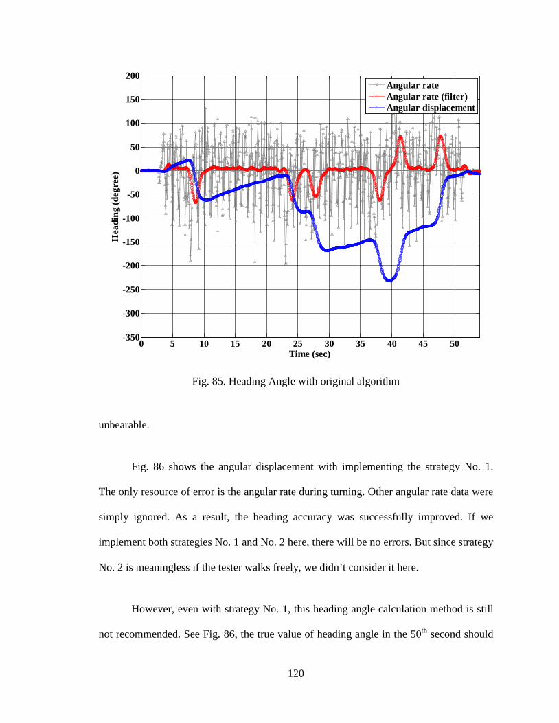
120

unbearable.

Fig. 86 shows the angular displacement with implementing the strategy No. 1.

The only resource of error is the angular rate during turning. Other angular rate data were

simply ignored. As a result, the heading accuracy was successfully improved. If we

implement both strategies No. 1 and No. 2 here, there will be no errors. But since strategy

No. 2 is meaningless if the tester walks freely, we didn’t consider it here.

However, even with strategy No. 1, this heading angle calculation method is still

not recommended. See Fig. 86, the true value of heading angle in the 50th

second should

Fig. 85. Heading Angle with original algorithm

0 5 10 15 20 25 30 35 40 45 50-350

-300

-250

-200

-150

-100

-50

0

50

100

150

200

Time (sec)

Hea

ding

(deg

ree)

Angular rateAngular rate (filter)Angular displacement

121

be minus 180 degree instead of minus 110 degree. 70 degree error is too large. Since

position is obtained from distance and heading angle, such result cannot be used for

positioning. This calculation method can only be used to find a probable value of heading

angle.

The next chapter describes the experiments and results. Based on the above

reasons, only the distance calculation results are shown here.

Fig. 86. Heading Angle with improved algorithm

0 5 10 15 20 25 30 35 40 45 50-350

-300

-250

-200

-150

-100

-50

0

50

100

150

200

Time (sec)

Hea

ding

(deg

ree)

Angular rateAngular rate (filter)Angular displacement

122

7.3.3 Experiments and Results

7.3.3.1 Experiment Conditions

• Route shape

The test route was designed exactly the same as Fig. 78. Hence it is easy to tell

the differences between two methods. The process is also the same as waist attached

IMU: a walking person walked from beginning point to the End point.

Fig. 87. Route for testing knee attached IMU

123

Note that there are two different sampling rates are used here. 19.7 Hz and 76.3

Hz (19.7 samples/second and 76.3 samples/second) .The results show trivial difference

between two sampling rates.

7.3.3.2 Results

Table 15. Distance Calculation (Knee Attached IMU) Tests Result I (S/R 19.7 Hz)

Data Files Conditions (True Values)

True Steps

Matlab program calculation Results

Steps Distance (m)

DATA_001

96.18 m six 90°

turnings, constant speed,

0 stops

124 125 94.14

Average = 96.29 m Standard

Deviation = 0.9977

Average = 96.19 m Standard

Deviation = 0.8840

DATA_003 124 124 96.17 DATA_003 125 127 96.99 DATA_004 124 123 97.70 DATA_005 124 125 95.66 DATA_006 122 121 96.17 DATA_007 125 127 96.45 DATA_008 125 125 96.69 DATA_009 126 127 97.25 DATA_010 124 123 95.72 DATA_011 96.18

six 90° turnings,

constant speed, 3 stops

125 138 97.69 Average = 96.62 m Stdev = 0.6563

DATA_012 125 138 96.03 DATA_013 123 136 96.67 DATA_014 125 138 96.54 DATA_015 125 136 96.15 DATA_016 96.18

six 90° turnings,

variable speed, 0 stops

124 123 96.21 Average = 95.56 m Stdev = 0.5431

DATA_017 121 121 95.26 DATA_018 120 121 94.87 DATA_019 120 119 95.48 DATA_020 122 121 95.99

The length of the test route is 96.18 m which is considered as true value. On the

right hand side of the above table, Matlab program gives the calculated distances.

DATA_001~010 are under constant walking speed without any stops conditions during

tests. DATA_011~015 are under constant walking speed with three stops conditions

124

during tests. DATA_016~020 are under variable walking speed without stops conditions

during tests. In fact, these conditions give little impact on the final results.

Table 16. Distance Calculation (Knee Attached IMU) Tests Result II (S/R 76.3 Hz)

Data Files Conditions True Steps

Matlab program calculation Results

Steps Distance (m)

11-12-2008-t2038.txt

96.18 m four 90° turnings, constant speed, 0 stops

125 125 95.88

Average = 97.87 m Standard Deviation

= 0.9196 Average =

97.66 m Standard

Deviation = 1.2684

11-12-2008-t2039.txt 124 125 98.60 11-12-2008-t2041.txt 123 123 98.60 11-12-2008-t2043.txt 123 123 97.77 11-14-2008-t1915.txt 125 125 97.75 11-14-2008-t1917.txt 125 125 97.26 11-14-2008-t1918.txt 127 127 98.53 11-14-2008-t1920.txt 129 129 99.10 11-14-2008-t1922.txt 127 127 97.86 11-14-2008-t1923.txt 125 125 97.38 11-12-2008-t2056.txt

variable speed

111 111 96.68 Average = 98.28 m Stdev = 0.2952

11-12-2008-t2057.txt 111 111 96.09 11-12-2008-t2058.txt 113 113 96.10 11-12-2008-t2100.txt 114 113 96.52 11-14-2008-t1925.txt 115 115 96.03 11-13-2008-t1835.txt 1 stop

2 stops 3 stops

127 128 98.14 99.22 m 1.0341 11-13-2008-t1837.txt 131 133 100.20

11-13-2008-t1839.txt 132 132 99.33

The only difference between Table 15 and 16 is the sampling rate. Obviously, the

results with higher sampling rate are a little larger than Table 15. But the error is still

acceptable. This is because higher sampling rate will introduce more noise.

No matter which sampling rate we use, the results from both Table 15 and 16 are

much better than the waist attached IMU.

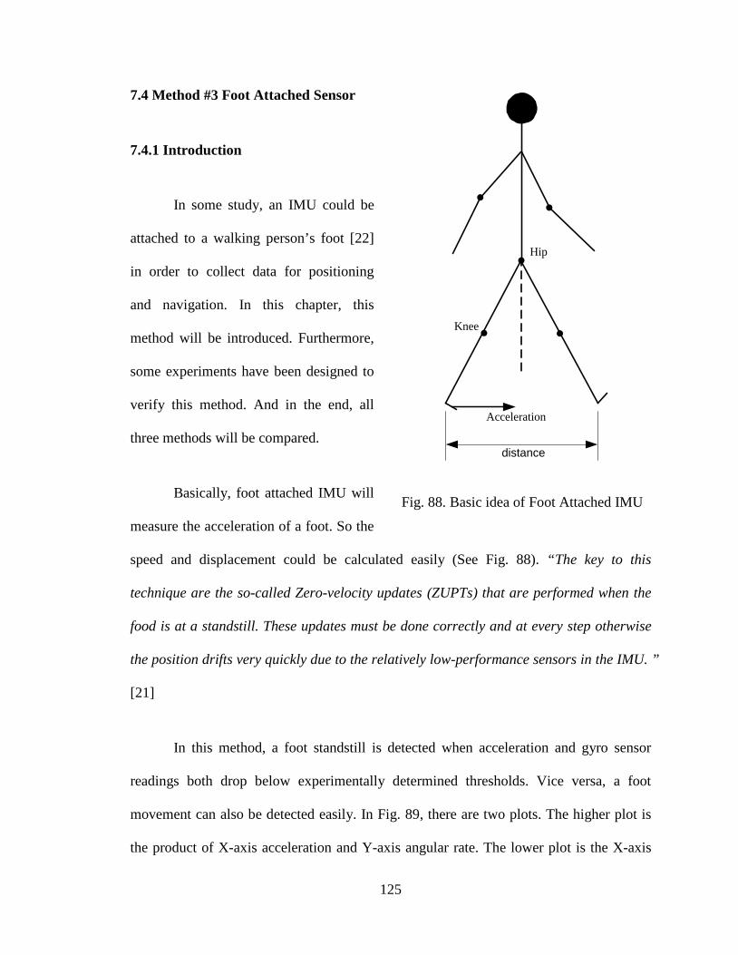
125

7.4 Method #3 Foot Attached Sensor

7.4.1 Introduction

In some study, an IMU could be

attached to a walking person’s foot [22]

in order to collect data for positioning

and navigation. In this chapter, this

method will be introduced. Furthermore,

some experiments have been designed to

verify this method. And in the end, all

three methods will be compared.

Basically, foot attached IMU will

measure the acceleration of a foot. So the

speed and displacement could be calculated easily (See Fig. 88). “The key to this

technique are the so-called Zero-velocity updates (ZUPTs) that are performed when the

food is at a standstill. These updates must be done correctly and at every step otherwise

the position drifts very quickly due to the relatively low-performance sensors in the IMU. ”

[21]

In this method, a foot standstill is detected when acceleration and gyro sensor

readings both drop below experimentally determined thresholds. Vice versa, a foot

movement can also be detected easily. In Fig. 89, there are two plots. The higher plot is

the product of X-axis acceleration and Y-axis angular rate. The lower plot is the X-axis

Hip

Knee

distance

Acceleration

Fig. 88. Basic idea of Foot Attached IMU

126

acceleration. Obviously, it is easier to determine the “standstill” period from the higher

plot. Once the “standstill” period has been determined, velocity is calculated by integral

on “movement” period. Furthermore, the velocity will be reset to zero whenever there is a

“standstill” period. By using this method, the drift could be bounded.

Fig. 90 shows the calculation results based on ZUPTs. The key of this method is

resetting velocity to zero after each “steps”. Without resetting, there will be a large bias

error in the distance calculation which will not be reliable in the end.

Fig. 89. Movement and Standstill

15 15.5 16 16.5 17 17.5 18 18.5 19 19.5 20-1000

0

1000

2000

3000

Prod

uct o

f X-a

xis a

ccel

erat

ion

and

Y-a

xis a

ngul

ar r

ate

15 15.5 16 16.5 17 17.5 18 18.5 19 19.5 20-6

-4

-2

0

2

4

Time (sec)

X-a

xis a

ccel

erat

ion

(G) 1st step

Standstill

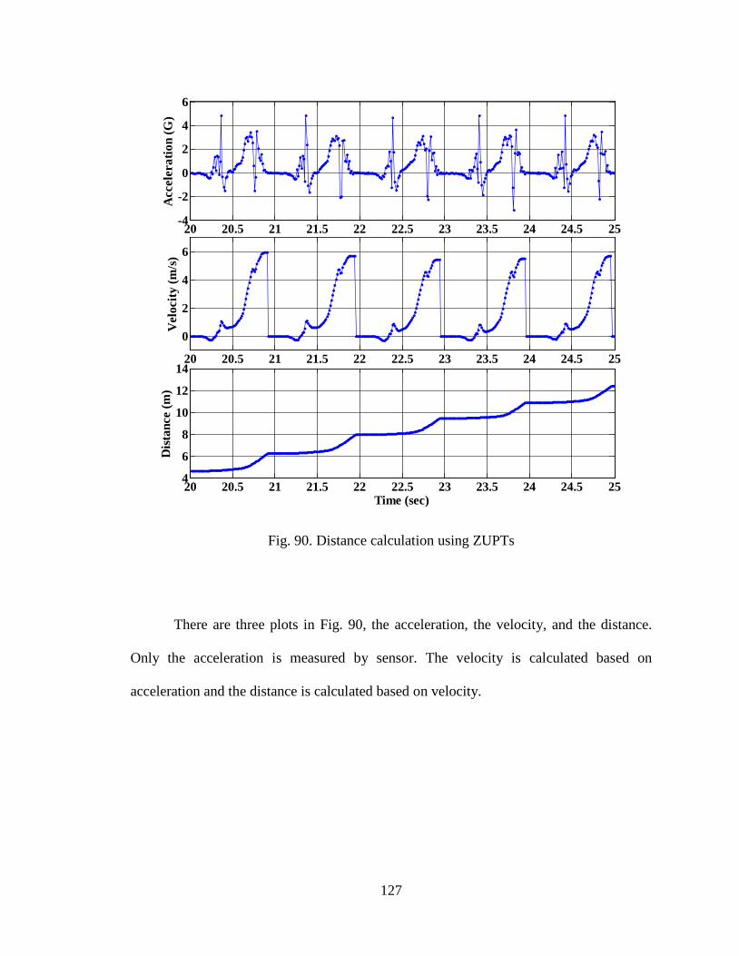
127

There are three plots in Fig. 90, the acceleration, the velocity, and the distance.

Only the acceleration is measured by sensor. The velocity is calculated based on

acceleration and the distance is calculated based on velocity.

Fig. 90. Distance calculation using ZUPTs

20 20.5 21 21.5 22 22.5 23 23.5 24 24.5 254

6

8

10

12

14

Dis

tanc

e (m

)

Time (sec)

20 20.5 21 21.5 22 22.5 23 23.5 24 24.5 25-4

-2

0

2

4

6

Acc

eler

atio

n (G

)

20 20.5 21 21.5 22 22.5 23 23.5 24 24.5 25

0

2

4

6

Vel

ocity

(m/s

)

128

7.4.3 Experiments & Results

7.4.3.1 Experiment Conditions

• Route shape

The test route was designed exactly the same as Fig. 78 and 87 (waist attached

IMU and knee attached IMU). Hence it is easy to tell the differences between all three

methods with the same benchmark. The process is also the same as waist attached IMU

and knee attached IMU: a walking person walked from beginning point to the End point.

Fig. 91. Route for testing knee attached IMU

129

Since the accuracy of distance calculation of waist attached IMU is unacceptable.

The comparison will be made between knee attached IMU and foot attached IMU in

Chapter 7.4.3.2.

7.4.3.2 Results

Table 17. Distance Calculation (Foot Attached IMU) Tests Result (S/R 76.3 Hz)

Data Files Conditions True Steps

Matlab program calculation Results

Steps Distance (m)

10-02-2008-t1943.txt

96.18 m four 90° turnings, constant speed, 0 stops

124 126 95.49

Average = 93.21 m Standard Deviation

= 3.5414 Average =

92.07 m Standard Deviation

= 3.8441

10-02-2008-t1948.txt 124 138 97.91 10-02-2008-t1954.txt 125 124 97.52 11-12-2008-t1618.txt 124 126 90.07 11-12-2008-t1620.txt 124 124 95.12 11-12-2008-t1624.txt 124 124 87.13 11-12-2008-t1626.txt 124 130 88.68 11-12-2008-t1628.txt 124 124 94.08 11-12-2008-t1629.txt 124 124 95.28 11-12-2008-t1631.txt 122 122 90.97 11-12-2008-t1634.txt 120 122 88.53 11-12-2008-t1636.txt 123 136 93.03 11-12-2008-t1652.txt 123 126 91.77 11-12-2008-t1654.txt 124 130 97.98 11-12-2008-t1656.txt 124 124 94.59 10-02-2008-t1950.txt 11-12-2008-t1714.txt 11-12-2008-t1716.txt 11-12-2008-t1722.txt 11-12-2008-t1724.txt 11-12-2008-t1726.txt 11-12-2008-t1727.txt

variable speed

120 124 94.20

Average = 88.75 m Stdev = 3.2333

112 134 90.82 112 118 90.33 113 126 87.86 112 124 85.74 112 120 84.97 112 114 87.30

11-12-2008-t1707.txt 11-12-2008-t1709.txt 11-12-2008-t1711.txt

1 stop 2 stops 3 stops

123 124 92.84 94.13 m 1.8466 124 126 96.24

125 130 93.30

130

From Table 16 and 17, it is obvious that knee attached IMU is better in distance

calculation. The true value is 96.18 m in all experiments. The knee attached IMU gives

96.19 m and 97.66 m as final results. On the other hand, the foot attached IMU gives

92.07 m as final result. Moreover, the standard deviation of Table 16 data is much

smaller than Table 17 data, which means the latter is neither stable nor accurate.

Fig. 92. Bar chart of average distance error of method #1~3

97.0

8

95.9

2

97.5

9

96.8

9

96.1

8

96.1

8

96.1

8

96.1

8

93.2

1

88.7

5 94.1

3

92.0

7

108.

55

105.

47

100.

26 105.

2980.00

85.00

90.00

95.00

100.00

105.00

110.00

115.00

120.00

125.00

Constant Speed w/o stops (15 trials)

Variable Speed w/o stops (7 trials)

Constant Speed w/ stops (7 trials)

Overall(29 trials)

Aver

age

Dist

ance

(m)

Type of Trials

Knee Attached IMUTrue ValueFoot Attached IMUWaist Attached IMU

1.23

62

3.54

14

9.43

17

0.56

09

3.23

33

10.5

236

1.84

46

5.76

73

1.54

03

1.30

01

3.84

41

10.9

000

131

7.5 Proposed Personal Navigation System and Test Results

Because the knee attached method gives the best performance in distance

calculation, and the waist attached method gives the best performance in heading

calculation, our proposed personal navigation system combines these two methods (See

Fig. 93). With the distance information coming from knee attached sensors, and the

heading information coming from the waist attached sensors, the current location of a

walking person can be obtained by dead reckoning (See Fig.2 in Chapter 2.3).

Fig. 93. Proposed Personal Navigation System

132

In the new personal navigation system, the NavBOARD is attached to the waist

and the IMU (3DM-GX1, see Chapter 2.3 for details) is attached to the knee. Fig. 94

shows the block diagram of the system. The NavBOARD will collect data from its own

onboard sensors and IMU. Then these data will be transfer to a desktop wirelessly.

Also, a series of experiments has been performed to test this system. The test

route is the same as before (See Fig. 95). Since the distance and heading information are

IMU(3DM-GX1) NavBOARD

Power

Data

Data(Wireless)

Desktop

Fig. 94. Block Diagram of Personal Navigation System

Fig. 95. Route for testing personal navigation system

133

both collected at this time, the goal of tracking a walking person can be achieved. Fig. 96

shows the tracking result. Table 18 shows the results of all twenty trials. The position

error is defined as the distance between the true “End” (See Fig. 95) and the calculated

“End” (See Fig. 96).

Fig. 96. Tracking a walking person result

-75.153 -75.1529 -75.1528 -75.1527 -75.1526 -75.1525

39.9821

39.9821

39.9822

39.9822

39.9823

39.9823

39.9824

39.9824

39.9825

Longitude (degree)

Lat

itude

(deg

ree)

True TraceTracking Result

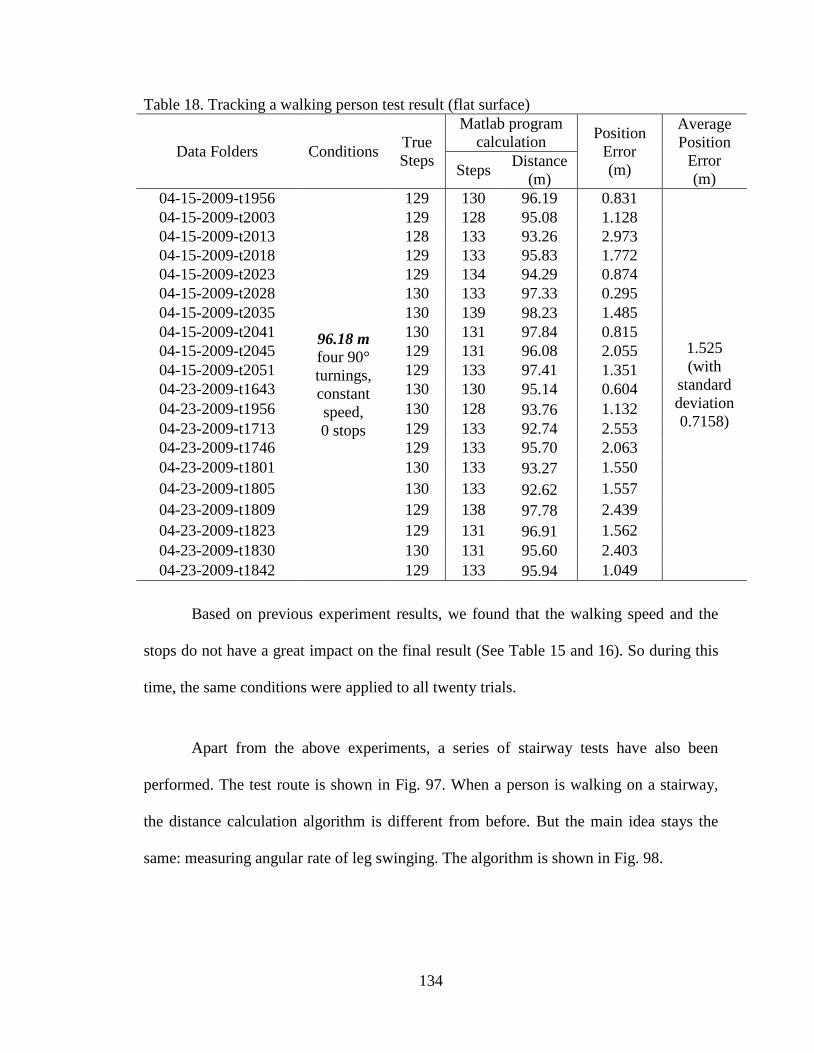
134

Table 18. Tracking a walking person test result (flat surface)

Data Folders Conditions True Steps

Matlab program calculation Position

Error (m)

Average Position

Error (m) Steps Distance

(m) 04-15-2009-t1956

96.18 m four 90° turnings, constant speed, 0 stops

129 130 96.19 0.831

1.525 (with

standard deviation 0.7158)

04-15-2009-t2003 129 128 95.08 1.128 04-15-2009-t2013 128 133 93.26 2.973 04-15-2009-t2018 129 133 95.83 1.772 04-15-2009-t2023 129 134 94.29 0.874 04-15-2009-t2028 130 133 97.33 0.295 04-15-2009-t2035 130 139 98.23 1.485 04-15-2009-t2041 130 131 97.84 0.815 04-15-2009-t2045 129 131 96.08 2.055 04-15-2009-t2051 129 133 97.41 1.351 04-23-2009-t1643 130 130 95.14 0.604 04-23-2009-t1956 130 128 93.76 1.132 04-23-2009-t1713 129 133 92.74 2.553 04-23-2009-t1746 129 133 95.70 2.063 04-23-2009-t1801 130 133 93.27 1.550 04-23-2009-t1805 130 133 92.62 1.557 04-23-2009-t1809 129 138 97.78 2.439 04-23-2009-t1823 129 131 96.91 1.562 04-23-2009-t1830 130 131 95.60 2.403 04-23-2009-t1842 129 133 95.94 1.049

Based on previous experiment results, we found that the walking speed and the

stops do not have a great impact on the final result (See Table 15 and 16). So during this

time, the same conditions were applied to all twenty trials.

Apart from the above experiments, a series of stairway tests have also been

performed. The test route is shown in Fig. 97. When a person is walking on a stairway,

the distance calculation algorithm is different from before. But the main idea stays the

same: measuring angular rate of leg swinging. The algorithm is shown in Fig. 98.

135

3.302 m

2.25

m

2.45 m

1.66 m

2.25

m2.

25 m

2.25

m

1.66 m

1.66 m

2.45 m

3.302 m

3.302 m

3.302 m

7th Floor

8th Floor

9th Floor

9 m

Begin

End

Fig. 97. Route for testing personal navigation system in stairway

136

In Fig. 98, α is the angular displacement of leg moving upstairs, h is the vertical

distance, and s is the horizontal distance. They could be calculated using (7.9) and (7.10).

( )( ) ( ) )9.7(5.0sincos12s αα ⋅⋅−⋅⋅= L

( )( ) ( ) )10.7(5.0coscos12h αα ⋅⋅−⋅⋅= L

Hip

Kneeα

thig

h le

ngth

h

h

s

L

Fig. 98. Leg movement of a walking person on wide stairs

137

Table 19. Tracking a walking person test result (stairway) I

Data Files Conditions True Steps

Measured Steps

Position Error (m)

Average Position

Error (m)

11-13-2008-t1843

See Fig. 97

69 69 0.57692

0.5501 (with standard

deviation 0.3199)

11-13-2008-t1850 69 69 0.55441 04-25-2009-t1923 69 69 0.12389 04-25-2009-t1933 69 69 0.69483 04-25-2009-t1940 69 69 0.78523 04-25-2009-t1951 69 69 0.93753 04-25-2009-t2005 69 69 0.82658 04-25-2009-t2017 69 69 0.66217 04-25-2009-t2029 69 69 0.95250 04-25-2009-t2040 69 69 1.12800 04-26-2009-t1603 69 69 0.62759 04-26-2009-t1616 69 69 0.21997 04-26-2009-t1625 69 69 0.21273 04-26-2009-t1639 69 69 0.21786 04-26-2009-t1650 69 69 0.55668 04-26-2009-t1659 69 69 0.21873 04-26-2009-t1709 69 69 0.99289 04-26-2009-t1723 69 69 0.16189 04-26-2009-t1734 69 69 0.22921 04-26-2009-t1748 69 69 0.32203

In Table 19, the Position Error is defined as the distance between the true “End”

(See Fig. 97) and the calculated “End” (See Fig. 99). Though the position error is less

than 1 meter in most tests, the tracking result is not actually “following” the true trace

(See Fig. 99). There exists a large horizontal error. However, because this is a “back and

forth” stairway, the horizontal error compensates itself as long as an even number of

“back and forth” has been performed.

138

Table 20. Tracking a walking person test result (stairway) II

Data Files Average

Horizontal Error (m)

Average Vertical

Error (m)

11-13-2008-t1843 1.0544 0.2835 11-13-2008-t1850 1.0902 0.2278 04-25-2009-t1923 1.0642 0.3053 04-25-2009-t1933 1.0700 0.2959 04-25-2009-t1940 1.0725 0.2456 04-25-2009-t1951 1.0769 0.3323 04-25-2009-t2005 1.1322 0.2033 04-25-2009-t2017 1.0240 0.3013 04-25-2009-t2029 0.9989 0.3135 04-25-2009-t2040 0.9393 0.5528 04-26-2009-t1603 1.0147 0.4019 04-26-2009-t1616 1.1329 0.3078 04-26-2009-t1625 1.1065 0.3594 04-26-2009-t1639 1.0271 0.3969 04-26-2009-t1650 0.9648 0.3628 04-26-2009-t1659 1.0440 0.3073 04-26-2009-t1709 1.0343 0.3312 04-26-2009-t1723 1.0816 0.4077 04-26-2009-t1734 0.9450 0.3738 04-26-2009-t1748

Average Standard deviation

1.0250 0.4586 1.0449 0.3384 0.0549 0.0808

Table 20 shows the average horizontal and vertical error. Instead of just using the

end location, Table 20 evaluates the whole result data set. The horizontal error is the

horizontal distance between each calculated position and true position. The vertical error

is the vertical distance between each calculated position and true position. As shown in

Table 20, the horizontal error is almost three times as the vertical error.

The reason for this can be explained with Fig. 100. In Fig. 98, an important

assumption has been made. That is the calf of a walking person in stairway is always

vertical to the ground. In another word, each stair is wide enough to let a person walking

139

with his/her calf vertical to the ground. However, if the stair is narrower as shown in Fig.

100, a person cannot achieve the same horizontal distance with the same leg swinging. As

a result, the angular displacement of the leg remains the same as well as the vertical

distance. But the horizontal distance shrinks. Unfortunately, because we cannot detect

whether the calf is vertical to the ground or not (the sensor is attached to the lower thigh

not the calf), the program still accept the assumption and calculated a larger horizontal

distance. This kind of error may be eliminated by using more sensors.

Fig. 99. Tracking a walking person result (stairway)

0 2 4 6 8 100

1

2

3

4

5

6

7

8

9

10

Horizontal distance (meter)

Ver

tical

dist

ance

(met

er)

Tracking ResultTrue Trace

140

On narrow stairs, a person will walk as shown in Fig. 100. Though the angular

displacement α and vertical distance h stay the same as in Fig. 98, the horizontal distance

is shorter. By using (7.9), the calculated horizontal distance will be larger than the true

value.

Hip

Kneeα

thig

h le

ngth

h

h

s

L

Fig. 100. Leg movement of a walking person on narrow stairs

141

7.6 Conclusions

A bar chart was organized as in Fig. 92 to show the experiment results leading to

the proposed personal navigation system. As indicated before, since the entire trail routes

are the same, the true value (length of the route) is 96.18 m for all tests (red bar in Fig.

92). There are four categories in this chart. The first three (from left to right) categories

are three different test conditions:

• Constant speed without stops

• Variable speed without stops

• Constant speed with stops

In each category, the chart shows the average distance and the standard deviation.

For example, the first category “Constant speed without stops”, 15 trials have been

carried out during the experiment. The average distance is 97.08 m for knee attached

IMU (blue bar) which is the closest to the true value 96.18 m and with the smallest

standard deviation. The last category named “Overall” is the average distance and

standard deviation of all the trials (15+7+7 = 29 trials). It is obvious that the 96.89 m blue

bar, knee attached IMU, is the most accurate one. On the other hand, the food attached

IMU is worse than the knee attached IMU in both average distance and standard

deviation. But it is better than waist attached IMU which has the largest error and

standard deviation.

Based on these tests results, a personal navigation system has been proposed. The

knee attached IMU is utilized to calculated the distance. And the waist attached IMU is

142

the only reasonable choice for heading calculation. A series of experiments has been

performed to test this personal navigation system in flat surface condition and in

stairways. The average error is 1.525 meters in flat surface condition, and 0.5501 meter

in stairways.

143

CHAPTER 8

CONCLUSIONS

8.1 Summary of Results and Conclusions

GPS signals are weak or even disappear in urban canyons, forests, and indoors.

Sometimes however, although GPS position information (Lat, Lon) is not reliable, GPS

ground speed or GPS heading information may still be useful.

Inertial sensors including accelerometers, gyroscopes and magnetometers can be

used to augment GPS. But they introduce cumulative errors in the long run. As a result,

we have to use GPS as much as possible or use GPS to update the results as long as GPS

position, GPS speed, GPS heading is reliable.

In summary, to enhance the navigation performance of GPS, we introduced a

novel data fusion method. Using this method, we demonstrate that the system works in a

stressed environment. Fused navigation data works better than GPS or IMU alone. In

most cases, the relative improvement is larger than 50% (See Fig. 46 and Table 10. The

concept of expert system works well as a data fusion method and the method can be

improved by modifying this. It can be used for automobile navigation, and uninhabited

autonomous vehicle navigation.

144

Also, an indoor experiment has been designed for testing the laser alignment idea.

Two parallel laser beams were used to aid the rolling cart to align with a preset direction.

By doing this, the heading angle could be reset every time the rolling cart passes the laser

beams. This method was proved to be valuable under indoor operation when there is no

GPS signal at all. The positioning error was bounded when this method is implemented.

Without it, the indoor positioning relying only on IMU is a disaster. The error will be

unbounded with the time increases.

Three personal navigation methods were introduced. By attaching an IMU device

on three different places of human body, a series of experiments have been designed to

verify these methods. In fact, the dynamic characteristics of a walking person have been

discussed here. Technically, in order to obtain the entire dynamic information of a

walking person, the IMU should be attached to the foot. The higher (body) the IMU is

attached, the less information it is obtained. This is the reason why a waist attached IMU

does not give good results. However, on the other hand, the lower (body) the IMU is

attached to, the larger the noise it receives. That is because the lower body, which sustain

the whole body, will undergo large amount of vibrations during walking. The feet

suffered the most from this error. If the IMU is attached to the foot, the measurements

will include all the vibration noises. Based on the test results, conclusions were drawn as

follows:

• The waist attached IMU cannot be used for distance calculation (with ErrorTrue value

∗

100% ≈ 12.5% ), but it is suitable for heading angle calculation

(with ErrorTrue value

∗ 100% ≈ 0.5%).

145

• The knee attached IMU shows the best result in distance calculation

(with ErrorTrue value

∗ 100% ≈ 1% ). But it is not suitable for heading angle

calculation (with ErrorTrue value

∗ 100% ≈ 39%).

• The foot attached IMU is better than waist attached IMU but worse than knee

attached IMU in distance calculation (with ErrorTrue value

∗ 100% ≈ 5%). It is also

not suitable for heading angle calculation (with ErrorTrue value

∗ 100% ≈ 45%).

After comparing these three methods, another personal navigation system has

been proposed. A knee attached IMU is utilized to calculate the distance. Another waist

attached IMU is utilized to calculate the heading. A microprocessor unit is used to

coordinate the two IMUs and send the packed data to a terminal wirelessly. A series of

experiments has been performed to test this personal navigation system in flat surface

condition and in stairways. The average error is 1.525 meters in flat surface condition (in

the 96.18 meters long test route shown in Fig. 91), and 0.5501 meter in stairways (in the

3-story test route shown in Fig. 97).

146

8.2 Suggestions for Future Work

After this research, some concerns are raised, and some suggestions have been

made.

1) The rules used in the research are extracted based on experiments, experiences, and

common senses. As a result, the reason of designing some specific rules is empirical

and experimental. And the solid connection between the rules and the accuracy of

measurement is unknown. Only by experiments, the effectiveness of the rules can be

examined. Further studies maybe required to reveal the connection between rules and

measurement accuracy.

2) The rules designed in this research are utilized to cover different situations. In other

words, different rules solve different problems. As a result, there are possibilities that

the existing rules can not deal with new situations. In this case, the original rule base

needs to be updated to adapt new situations. Currently there are two hundred and

seventy rules in our rule base. If this rule base will be updated in the future, a more

efficient structure maybe needed to organize the rule base.

3) The robustness of our navigation system depends not only on the rule base, but also

on the accuracy of inertial sensors and GPS receiver. Since the size of the system is

critical for us, miniature MEMS sensors are used. Apart from its small size and

simple operation, MEMS sensors still cannot achieve high accuracy comparing to

some traditional inertial sensors. In addition, since GPS receiver lost satellite

reception even without stressed environments, multiple GPS receivers working

simultaneously maybe necessary in further study.

147

4) The mobile platform consist the NavBOX and a rolling cart. The rolling cart can be

redesigned to an unmanned vehicle or a self-navigated robot. A control unit is

required for this kind of action. In addition, the mobile platform used in this research

was not able to complete Real Time Data Process. Instead, it just collects and stores

all the date for post-process. A reliable Real Time Data Process algorithm is highly

demanding. The post-process program, which is in Matlab, can be rewritten as a real-

time data process program in the future.

5) Though we reached the conclusion that the knee attached sensor and the waist

attached sensor have to be used together, the heading calculation is still not reliable

since heading error is cumulative after each turn. In addition, it is better that the knee

attached sensor is designed as a wireless module as well as the waist attached sensor

since this can reduce the wire attached to human body. It is acceptable to attach a

module (without wired connections) to human body without confining movements.

However, wired connections attached to human body could greatly reduce our ability

to move freely.

148

REFER4ENCES

[1] GPS Sensor Boards GPS25-LVC Technical Specification, Garmin International,

Inc, pp. 4, 2000.

[2] LassenTM

[3] Alison K. Brown and Y. Lu, “Performance Test Results of an Integrated

GPS/MEMS Inertial Navigation Package,” Proceedings of ION GNSS 2004, Long

Beach, California, September 2004.

SQ GPS Receiver System Designer Reference Manual, Trimble, pp.

154, 2002.

[4] Alison K. Brown and Y. Lu, “Indoor Navigation Test Results using an Integrated

GPS/TOA/Inertial Navigation System,” Proceedings of ION GNSS 2006, Fort

Worth, Texas, September 2006.

[5] R. Muellerschoen, Michael Armatys, “Aviation Applications of NASA’s Global

Differential GPS System,” 2nd AIAA "Unmanned Unlimited" Systems,

Technologies, and Operations — Aerospace, Land, and Sea Conference and

Workshop & Exhibit, San Diego, California, September 2003.

[6] J. A. Farrell and M. Barth, The Global Positioning System and Inertial Navigation.

McGraw-Hill, New York, NY, 1999.

[7] Mohinder S. Grewal and L. R. Weill, Global Position Systems, Inertial

Navigation, and Integration. Wiley-Interscience, John Wiley & Sons, Inc, 2007.

[8] Hanching Grant Wang and Thomas C. Williams, “Strategic Inertial Navigation

Systems,” in IEEE Control Syst. Mag., pp. 69, February, 2008.

149

[9] Eric Abbott and David Powell, “Land-Vehicle Navigation Using GPS,” in Proc.

of the IEEE, Vol. 87, No. 1, January 1999.

[10] Wang Bin, Wang Jian, Wu Jianping and Cai Baigen, “Study on Adaptive

GPS/INS Integrated Navigation System,” IEEE Trans. Intell. Transp. Syst., Vol. 2,

pp. 1016-1021, October, 2003.

[11] Salah Sukkarieh, Eduardo M. Nebot and Hugh F. Durrant-Whyte, “A high

Integrity IMU/GPS Navigation Loop for Autonomous Land Vehicle

Applications”, IEEE Trans. Robot. Autom., Vol. 15, No. 3, June 1999.

[12] A. H. Mohamed and K. P. Schwarz, “Adaptive Kalman Filtering for INS/GPS,”

Journal of Geodesy, pp. 193-203, 1999

[13] Shu-Hsien Liao, “Expert system methodologies and applications — a decade

review from 1995 to 2004,” Expert System with Applications, 28, pp. 93-103,

2005.

[14] David L. Hall and James Llinas, “An Introduction to Multisensor Data Fusion,” in

Proc. of the IEEE, Vol. 85, No. 1, January 1997.

[15] Trudi Farrington-Darby and John R. Wilson, “The nature of expertise: A review,”

Applied Ergonomics, 37, pp. 17-32, 2006.

[16] Liang-Tu Song, Xian-Ping Liu, Jin-Yuan Bi, Jin-Shui Zha, “A rule-based expert

system with multiple knowledge databases,” Pattern Recognition and Artificial

Intelligence, Vol. 19, No 4, pp. 515-519, 2006.

[17] Joseph C. Giarratano and Gary D. Riley, Expert System, Principles and

Programming. Thomson Course Technology, Boston, MA, 2005.

150

[18] Harvey Weinberg, “AN-602: Using the ADXL202 in Pedometer and Personal

Navigation Applications”

http://www.analog.com/UploadedFiles/Application_Notes/513772624AN602.pdf

[19] Masakatsu Kourogi and Takeshi Kurata, “Personal Positioning based on Walking

Locomotion Analysis with Self-Contained Sensors and a Wearable Camera,”

Proceedings of the Second IEEE and ACM International Symposium on Mixed

and Augmented Reality 2003 (ISMAR’03), Washington, United States.

[20] Koichi Sagawa, Hikaru Inooka, and Yutaka Satoh, “Non-restricted Measurement

of Walking Distance,” In Proceedings IEEE International Conference on Systems,

Man, and Cybernetics, 2000

[21] Eric Foxlin, “Pedestrian Tracking with Shoe-Mounted Inertial Sensors,” IEEE

Computer Society, 2005

[22] Stephane Beauregard, “Omnidirectional Pedestrian Navigation for First

Responders,” 4th

[23] Akihiro Hamaguchi, Masayuki Kanbara, and Naokazu Yokoya, “User

Localization Using Wearable Electromagnetic Tracker and Orientation Sensor,”

IEEE, 2006

Workshop on Positioning, Navigation and Communication 2007

(WPNC’ 07), Hannover, Germany.

[24] Ryuhei Tenmoku, Masayuki Kanbara, and Naokazu Yokoya, “A wearable

Augmented Reality System for Navigation Using Positioning Infrastructures and

a Pedometer,” Proceedings of the Second IEEE and ACM International

Symposium on Mixed and Augmented Reality 2003 (ISMAR’03), Washington,

United States.

151

[25] Rabbit 3000 Microprocessor User's Manual, Rabbit Semiconductor, 2005

[26] Vincenty, T., (1975). Direct and inverse solutions of geodesics on the ellipsoid

with application of nested equations, Survey Review 23, Number 176, p 88-93

152

BIBLIOGRAPHY

Abbott Eric and Powell David. Land-Vehicle Navigation Using GPS. In Proc. of the

IEEE, Vol. 87, No. 1, January 1999.

Akihiro Hamaguchi, Masayuki Kanbara, and Naokazu Yokoya. User Localization Using

Wearable Electromagnetic Tracker and Orientation Sensor. In Proceedings IEEE

International Symposium on Wearable Computers, pages 55-58, 2006

Beauregard Stephane. Omnidirectional Pedestrian Navigation for First Responders. In 4th

Workshop on Positioning, Navigation and Communication 2007 (WPNC’ 07), Hannover,

Germany.

Brown Alison K. and Lu Y. Indoor Navigation Test Results using an Integrated

GPS/TOA/Inertial Navigation System. In Proceedings of ION GNSS 2006, Fort Worth,

Texas, September 2006.

Brown Alison K. and Lu Y. Performance Test Results of an Integrated GPS/MEMS

Inertial Navigation Package. In Proceedings of ION GNSS 2004, Long Beach, California,

September 2004.

Farrell J. A. and Barth M. The Global Positioning System and Inertial Navigation.

McGraw-Hill, New York, NY, 1999.

153

Foxlin Eric. Pedestrian Tracking with Shoe-Mounted Inertial Sensors. In Computer

Graphics and Applications, IEEE, 25:38-46, 2005.

Giarratano Joseph C. and Riley Gary D. Expert System, Principles and Programming.

Thomson Course Technology, Boston, MA, 2005.

Grewal Mohinder S. and Weill L. R. Global Position Systems, Inertial Navigation, and

Integration. Wiley-Interscience, John Wiley & Sons, Inc, 2007.

Hall David L. and Llinas James. An Introduction to Multisensor Data Fusion. in Proc. of

the IEEE, Vol. 85, No. 1, January 1997.

Koichi Sagawa, Hikaru Inooka, and Yutaka Satoh. Non-restricted Measurement of

Walking Distance. In Proceedings IEEE International Conference on Systems, Man, and

Cybernetics, 2000.

Liang-Tu Song, Xian-Ping Liu, Jin-Yuan Bi, Jin-Shui Zha. A rule-based expert system

with multiple knowledge databases. In Pattern Recognition and Artificial Intelligence,

Vol. 19, No 4, pp. 515-519, 2006.

Liao Shu-Hsien. Expert system methodologies and applications — a decade review from

1995 to 2004. In Expert System with Applications, 28, pp. 93-103, 2005.

Masakatsu Kourogi and Takeshi Kurata. Personal Positioning based on Walking

Locomotion Analysis with Self-Contained Sensors and a Wearable Camera. In

154

Proceedings of the Second IEEE and ACM International Symposium on Mixed and

Augmented Reality 2003 (ISMAR’03), Washington, United States.

Mohamed A. H. and Schwarz K. P. Adaptive Kalman Filtering for INS/GPS. In Journal

of Geodesy, pp. 193-203, 1999.

Muellerschoen R. and Armatys Michael. Aviation Applications of NASA’s Global

Differential GPS System. In 2nd AIAA "Unmanned Unlimited" Systems, Technologies,

and Operations — Aerospace, Land, and Sea Conference and Workshop & Exhibit, San

Diego, California, September 2003.

Ryuhei Tenmoku, Masayuki Kanbara, and Naokazu Yokoya. A wearable Augmented

Reality System for Navigation Using Positioning Infrastructures and a Pedometer. In

Proceedings of the Second IEEE and ACM International Symposium on Mixed and

Augmented Reality 2003 (ISMAR’03), Washington, United States.

Salah Sukkarieh, Eduardo M. Nebot and Hugh F. Durrant-Whyte. A high Integrity

IMU/GPS Navigation Loop for Autonomous Land Vehicle Applications. In IEEE Trans.

Robot. Autom., Vol. 15, No. 3, June 1999.

Trudi Farrington-Darby and Wilson, John R. The nature of expertise: A review. In

Applied Ergonomics, 37, pp. 17-32, 2006.

Vincenty, T., (1975). Direct and inverse solutions of geodesics on the ellipsoid with

application of nested equations, Survey Review 23, Number 176, p 88-93

155

Wang Bin, Wang Jian, Wu Jianping and Cai Baigen. Study on Adaptive GPS/INS

Integrated Navigation System. In IEEE Trans. Intell. Transp. Syst., Vol. 2, pp. 1016-1021,

October, 2003.

Wang Hanching Grant and Williams Thomas C. Strategic Inertial Navigation Systems. In

IEEE Control Syst. Mag., pp. 69, February, 2008.

Weinberg Harvey. AN-602: Using the ADXL202 in Pedometer and Personal Navigation

Applications.

http://www.analog.com/UploadedFiles/Application_Notes/513772624AN602.pdf

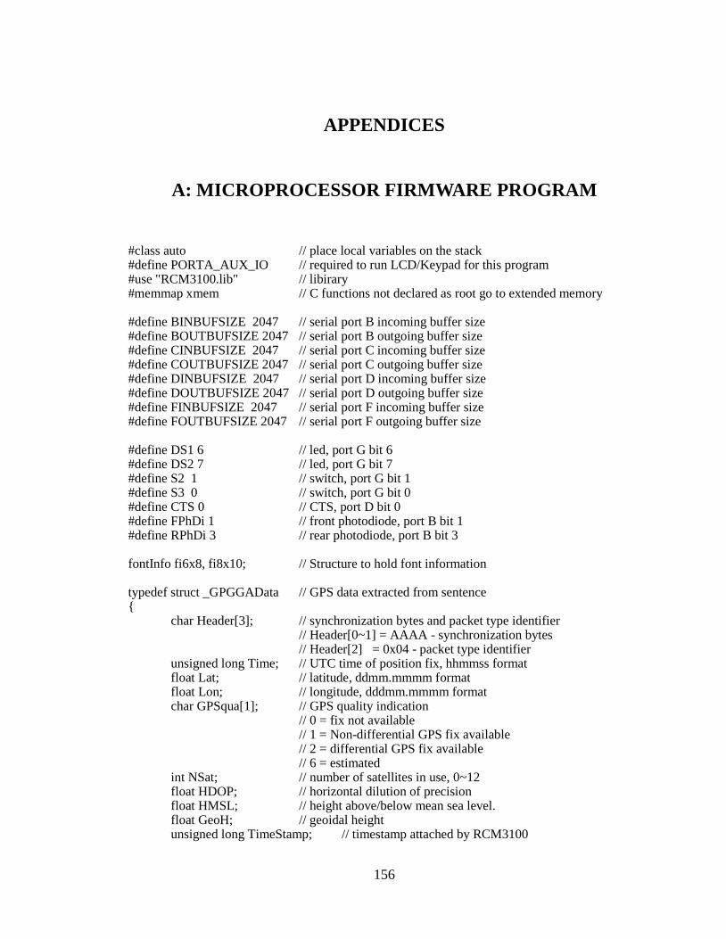
156

APPENDICES

A: MICROPROCESSOR FIRMWARE PROGRAM

#class auto // place local variables on the stack #define PORTA_AUX_IO // required to run LCD/Keypad for this program #use "RCM3100.lib" // libirary #memmap xmem // C functions not declared as root go to extended memory #define BINBUFSIZE 2047 // serial port B incoming buffer size #define BOUTBUFSIZE 2047 // serial port B outgoing buffer size #define CINBUFSIZE 2047 // serial port C incoming buffer size #define COUTBUFSIZE 2047 // serial port C outgoing buffer size #define DINBUFSIZE 2047 // serial port D incoming buffer size #define DOUTBUFSIZE 2047 // serial port D outgoing buffer size #define FINBUFSIZE 2047 // serial port F incoming buffer size #define FOUTBUFSIZE 2047 // serial port F outgoing buffer size #define DS1 6 // led, port G bit 6 #define DS2 7 // led, port G bit 7 #define S2 1 // switch, port G bit 1 #define S3 0 // switch, port G bit 0 #define CTS 0 // CTS, port D bit 0 #define FPhDi 1 // front photodiode, port B bit 1 #define RPhDi 3 // rear photodiode, port B bit 3 fontInfo fi6x8, fi8x10; // Structure to hold font information typedef struct _GPGGAData // GPS data extracted from sentence { char Header[3]; // synchronization bytes and packet type identifier // Header[0~1] = AAAA - synchronization bytes // Header[2] = 0x04 - packet type identifier unsigned long Time; // UTC time of position fix, hhmmss format float Lat; // latitude, ddmm.mmmm format float Lon; // longitude, dddmm.mmmm format char GPSqua[1]; // GPS quality indication // 0 = fix not available // 1 = Non-differential GPS fix available // 2 = differential GPS fix available // 6 = estimated int NSat; // number of satellites in use, 0~12 float HDOP; // horizontal dilution of precision float HMSL; // height above/below mean sea level. float GeoH; // geoidal height unsigned long TimeStamp; // timestamp attached by RCM3100

157

}GPGGAData, *pGPGGAData; // 34 bytes typedef struct _GPGSAData // GPS data extracted from sentence { char Header[3]; // synchronization bytes and packet type identifier // Header[0~1] = AAAA - synchronization bytes // Header[2] = 0x05 - packet type identifier char Mode[1]; // M = manual // A = automatic char Ftype[1]; // fix type // 1 = not available // 2 = 2D // 3 = 3D char PRN[12]; // PRN number, 1~32, of satellite used in solution // up to 12 transmitted float PDOP; // position dilution of precision float HDOP; // horizontal dilution of precision float VDOP; // vertical dilution of precision unsigned long TimeStamp; // timestamp attached by RCM3100 }GPGSAData, *pGPGSAData; // 33 bytes typedef struct _GPRMCData // GPS data extracted from sentence { char Header[3]; // synchronization bytes and packet type identifier // Header[0~1] = AAAA - synchronization bytes // Header[2] = 0x06 - packet type identifier unsigned long Time; // UTC time of position fix, hhmmss format char Status[1]; // A = valid position // V = NAV receiver warning float Lat; // latitude, ddmm.mmmm format float Lon; // longitude, dddmm.mmmm format float GSpeed; // speed over ground float Heading; // course over ground unsigned long Date; // UTC date of position fix, ddmmyy format float MagVar; // magnetic variation char MagVarD[1]; // magnetic veriation direction // E = East // W = West char Mode[1]; // mode indicator // A = autonomous // D = differential // E = estimated // N = data not valid unsigned long TimeStamp;// timestamp attached by RCM3100 }GPRMCData, *pGPRMCData; // 38 bytes typedef struct _PGRMEData // GPS data extracted from sentence { char Header[3]; // synchronization bytes and packet type identifier // Header[0~1] = AAAA - synchronization bytes // Header[2] = 0x07 - packet type identifier float EHPE; // estimated horizontal position error float EVPE; // estimated vertical position error float EPE; // estimated position error

158

unsigned long TimeStamp;// timestamp attached by RCM3100 }PGRMEData, *pPGRMEData; // 19 bytes typedef struct _IMUData // IMU data { char Header[2]; // synchronization bytes char Data[23]; // IMU data float Speed; // walking speed unsigned long TimeStamp;// timestamp attached by RCM3100 }IMUData, *pIMUData; // 33 bytes typedef enum _STATUS { STATUS_FAIL = 0, STATUS_OK = 1 }STATUS; GPGGAData GPGGA; // define structure GPGSAData GPGSA; // define structure GPRMCData GPRMC; // define structure PGRMEData PGRME; // define structure IMUData IMU; // define structure unsigned long IMUi; // number of data unsigned long GPSi; // number of data char IMU_Buffer[23]; // data buffer used during serial port reading/sending char GPS_Buffer[128]; // data buffer used during serial port reading/sending unsigned long StWa; // stopwatch - save the current time (sec) char IMUPacketType[1]; // handshake commamd with IMU char GPSPacketTypeCode[6]; // GPS NMEA 0183 header GP*** int DataLength; // 23 bytes as a IMU original packet unsigned long CountW; unsigned long Time0; unsigned long TimeInterval; float Speedms; float Speedkmh; void SpeedMeasurement(); /* ------------------------------------------------------------------------ -- -- Function : STATUS CheckLaserAlign(void) -- -- Description : to see if aligned -- -- ------------------------------------------------------------------------ */ STATUS CheckLaserAlign(void) { unsigned int DioA, DioB; DioA = BitRdPortI(PDDR, FPhDi); DioB = BitRdPortI(PDDR, RPhDi); return (DioA && DioB) ? (STATUS_OK) : (STATUS_FAIL); } /* ------------------------------------------------------------------------ -- -- Function : viod ReadIMUDataFromSerialPortC(void) --

159

-- Description : read the IMU data from serial port C -- -- ------------------------------------------------------------------------ */ void ReadIMUDataFromSerialPortC(char Command) { int n; n = 0; serCputc(Command); // handshake command require IMU to send data do { n = serCread(IMU.Data, DataLength, 500); // read 23 bytes from port C }while(n != DataLength); // if read fails, keep reading } /* ------------------------------------------------------------------------ -- -- Function : void SendIMUData2SerialPortD(void) -- -- Description : send the IMU data to Serial Port D -- -- ------------------------------------------------------------------------ */ void SendIMUData2SerialPortDF(void) { int i; if(DataLength != 23) // some IMU packets are smaller than 23 bytes { for(i = DataLength; i < 23; i++) { IMU.Data[i] = 0; // use 0 to fill up the empty spaces } } if(TimeInterval != 0) // three spokes in the wheel { // 0.3254 is 1/3 perimeter Speedms = 0.3254 / ((float)TimeInterval / 1000); Speedkmh = Speedms * 3.6; } else { Speedms = Speedms; // keep last value Speedkmh = Speedkmh; // keep last value } IMU.TimeStamp = MS_TIMER; // record current time in ms if(IMU.TimeStamp - Time0 < 1500) { IMU.Speed = Speedkmh; // record speed data (km/h) } else { IMU.Speed = 0; } if(CheckLaserAlign()) // laser aligned { for(i = 1; i < 7; i++) { IMU.Data[i] = 0; // reset roll, pitch and yaw to 0 }

160

BitWrPortI(PGDR, &PGDRShadow, 0, DS2); // LED2 on } else { BitWrPortI(PGDR, &PGDRShadow, 1, DS2); // LED2 off } serDwrite(&IMU, 33); // send 33 bytes IMU data to serial port D IMUi++; if(BitRdPortI(PDDR, CTS) != 1) // when CTS = 1, the transcevier is not ready to { // accept the data from Rabbit serFwrite(&IMU, 33); // send 33 bytes IMU data to serial port F } } /* ------------------------------------------------------------------------ -- -- Function : viod ReadGPSDataFromSerialPortB(void) -- -- Description : read the GPS data from serial port B -- -- ------------------------------------------------------------------------ */ void ReadGPSDataFromSerialPortB(void) { int i, c, k; c = serBgetc(); // read one byte from GPS i = 0; while(c != '$') // '$' is the first character of every NMEA sentance { c = serBgetc(); // find the begining of one sentance } do { if(c != -1) // c = -1 means no byte read from GPS { GPS_Buffer[i] = c; i++; } c = serBgetc(); } while(c != 0x0A); // 0x0A --- <LF> // <LF> is the last character of every NMEA sentance GPS_Buffer[i] = c; // GPS_Buffer[i] = <LF> GPS_Buffer[i + 1] = '\0'; // indicates the end of an array, otherwise the following program } // will not recognise this array correctly /* ------------------------------------------------------------------------ -- -- Function : viod GetGPSPacketType(void) -- -- Description : get GPS packet type from NMEA sentence header -- -- ------------------------------------------------------------------------ */ int GetGPSPacketType(char *code) { if(!strcmp(code, "GPGGA")) { return 4; // GPGGA - type 4 } if(!strcmp(code, "GPGSA")) { return 5; // GPGSA - type 5

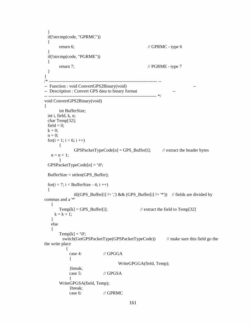
161

} if(!strcmp(code, "GPRMC")) { return 6; // GPRMC - type 6 } if(!strcmp(code, "PGRME")) { return 7; // PGRME - type 7 } } /* ------------------------------------------------------------------------ -- -- Function : void ConvertGPS2Binary(void) -- -- Description : Convert GPS data to binary format -- -- ------------------------------------------------------------------------ */ void ConvertGPS2Binary(void) { int BufferSize; int i, field, k, n; char Temp[32]; field = 0; k = 0; n = 0; for(i = 1; i < 6; i ++) { GPSPacketTypeCode[n] = GPS_Buffer[i]; // extract the header bytes n = n + 1; } GPSPacketTypeCode[n] = '\0'; BufferSize = strlen(GPS_Buffer); for(i = 7; i < BufferSize - 4; i ++) { if((GPS_Buffer[i] != ',') && (GPS_Buffer[i] != '*')) // fields are divided by commas and a '*' { Temp[k] = GPS_Buffer[i]; // extract the field to Temp[32] k = k + 1; } else { Temp[k] = '\0'; switch(GetGPSPacketType(GPSPacketTypeCode)) // make sure this field go the the write place { case 4: // GPGGA { WriteGPGGA(field, Temp); }break; case 5: // GPGSA { WriteGPGSA(field, Temp); }break; case 6: // GPRMC

162

{ WriteGPRMC(field, Temp); }break; case 7: // PGRME { WritePGRME(field, Temp); }break; } field = field + 1; k = 0; } } } /* ------------------------------------------------------------------------ -- -- Function : void SendGPSData2SerialPortD(void) -- -- Description : send the GPS data to Serial Port D -- -- ------------------------------------------------------------------------ */ void SendGPSData2SerialPortDF(void) { switch(GetGPSPacketType(GPSPacketTypeCode)) { case 4: { GPGGA.TimeStamp = MS_TIMER; // record current time in ms serDwrite(&GPGGA, 34); // send GPGGA GPSi++; if(BitRdPortI(PDDR, CTS) != 1) // when CTS = 1, the transcevier is not ready to { // accept the data from Rabbit serFwrite(&GPGGA, 34); // send GPGGA } }break; case 5: { GPGSA.TimeStamp = MS_TIMER; // record current time in ms serDwrite(&GPGSA, 33); // send GPGSA if(BitRdPortI(PDDR, CTS) != 1) // when CTS = 1, the transcevier is not ready to { // accept the data from Rabbit serFwrite(&GPGSA, 33); // send GPGSA } }break; case 6: { GPRMC.TimeStamp = MS_TIMER; // record current time in ms serDwrite(&GPRMC, 38); // send GPRMC if(BitRdPortI(PDDR, CTS) != 1) // when CTS = 1, the transcevier is not ready to { // accept the data from Rabbit serFwrite(&GPRMC, 38); // send GPRMC } }break; case 7: {

163

PGRME.TimeStamp = MS_TIMER; // record current time in ms serDwrite(&PGRME, 19); // send PGRME if(BitRdPortI(PDDR, CTS) != 1) // when CTS = 1, the transcevier is not ready to { // accept the data from Rabbit serFwrite(&PGRME, 19); // send PGRME } }break; } } /* ------------------------------------------------------------------------ -- -- Function : void SetPrintPacketType(int PT) -- -- Description : Display packet type on LCD -- -- ------------------------------------------------------------------------ */ void SetPacketType(int PT, char *HSIMU) { glPrintf (0, 0, &fi6x8, " Packet Type: "); switch(PT) { case 0: // Packet Type 0 { HSIMU[0] = 0x01; // The IMU will transmit the raw sensor output voltage DataLength = 23; // set packet size glPrintf (0, 8, &fi6x8, " 0x01 Raw Data "); }break; case 1: // Packet Type 1 { HSIMU[0] = 0x02; // The IMU will transmit the gyro-stabilized vectors DataLength = 23; // set packet size glPrintf (0, 8, &fi6x8, " 0x02 Gyro-Stab(GS) "); }break; case 2: // Packet Type 2 { HSIMU[0] = 0x03; // The IMU will transmit the instantaneous vectors DataLength = 23; // set packet size glPrintf (0, 8, &fi6x8, " 0x03 InstantVectors"); }break; case 3: // Packet Type 3 { HSIMU[0] = 0x0D; // The IMU will transmit the instantaneous Euler Angles DataLength = 11; // set packet size glPrintf (0, 8, &fi6x8, " 0x0D Instant EA "); }break; case 4: // Packet Type 4 { HSIMU[0] = 0x31; // The IMU will transmit gyro-stabilized Euler Angles DataLength = 23; // set packet size glPrintf (0, 8, &fi6x8, " 0x31 GSEA, IA, CAR "); // instantaneous acceleration }break; // drift compensated angular rate } } /* ------------------------------------------------------------------------ --

164

-- Function : SystemInit -- -- Description : NavBOX System Initialization -- -- ------------------------------------------------------------------------ */ void SystemInit(void) { static int wKey; // int for saving key action int PacketType; // 4 types of packet DataLength = 23; // default packet size IMUPacketType[0] = 0x31; // default packet type PacketType = 3; // default packet type No. brdInit(); // prototype board I/O initialization dispInit(); // LCD display initialization CountW = 0; // speed measurement module initialization Time0 = 0; // speed measurement module initialization TimeInterval = 0; // speed measurement module initialization Speedms = 0; // speed measurement module initialization Speedkmh = 0; // speed measurement module initialization GPGGA.Header[0] = 0xAA; // synchronization bytes GPGGA.Header[1] = 0xAA; // synchronization bytes GPGGA.Header[2] = 0x04; // packet type identifier GPGSA.Header[0] = 0xAA; // synchronization bytes GPGSA.Header[1] = 0xAA; // synchronization bytes GPGSA.Header[2] = 0x05; // packet type identifier GPRMC.Header[0] = 0xAA; // synchronization bytes GPRMC.Header[1] = 0xAA; // synchronization bytes GPRMC.Header[2] = 0x06; // packet type identifier PGRME.Header[0] = 0xAA; // synchronization bytes PGRME.Header[1] = 0xAA; // synchronization bytes PGRME.Header[2] = 0x07; // packet type identifier IMU.Header[0] = 0xAA; // synchronization bytes IMU.Header[1] = 0xAA; // synchronization bytes keyConfig ( 2, 'D', '3', 0, 0, 0, 0 ); // initialize key pad keyConfig ( 1, 'U', '5', 0, 0, 0, 0 ); // initialize key pad glXFontInit(&fi6x8, 6, 8, 32, 127, Font6x8); // initialize 6x8 font glXFontInit(&fi8x10, 8, 10, 32, 127, Font8x10); // initialize 8x10 font glBlankScreen(); serBopen(9600); // baud 9600 with GPS serCopen(19200); // baud 19200 with IMU serDopen(9600); // baud 9600 with PDA serFopen(9600); // baud 9600 with RF

165

IMUi = 0; // initialize IMU packet counter GPSi = 0; // initialize GPS packet counter BitWrPortI(PGDR, &PGDRShadow, 0, DS1); // LED1 on BitWrPortI(PGDR, &PGDRShadow, 1, DS2); // LED2 off ipset(1); // Dynamic C expands this call inline. // Replaces current interrupt priority // with another by rotatingthe new // priority into the IP register. WrPortI(PEDR, &PEDRShadow, 0x00); // set all E port pins low WrPortI(PEDDR, &PEDDRShadow, 0xCF); // set E port pin 4 & 5 as input '11001111' SetVectExtern3000(1, SpeedMeasurement); // set one of the external interrupt jump table entries WrPortI(I1CR, NULL, 0x21); // enable external INT1 on PE5, rising edge, priority 1 // '00100001' ipres(); // Dynamic C expands this call inline. // Restore previous interrupt priority // by rotating the IP register. glPrintf (0, 0, &fi6x8, " CSNAP - NavBOX "); // LCD display glPrintf (0, 8, &fi6x8, " DAQ System "); glPrintf (0, 16, &fi6x8, " By Zexi Liu "); glPrintf (0, 24, &fi6x8, " Press S2 to begin! "); while (BitRdPortI(PGDR, S2) == 1) // wait for switch S2 press { keyProcess(); // detecting key action if((wKey = keyGet()) != 0) // if keys are pressed { // wKey is the place to store the pressed key while(wKey == 'D' || wKey == 'U') { switch(wKey) // different procedure for different situation { case 'U': // increase PacketType No. { PacketType = PacketType + 1; if(PacketType > 4) // No.0 ~ 4 { PacketType = 0; } SetPacketType(PacketType, IMUPacketType); wKey = 0; }break; case 'D': // decrease PacketType No. {

166

PacketType = PacketType - 1; if(PacketType < 0) // No.0 ~ 4 { PacketType = 4; } SetPacketType(PacketType, IMUPacketType); wKey = 0; }break; } } } } // if S2 is pressed, begin DAQ glBlankScreen(); StWa = SEC_TIMER; // initialize stopwatch } /* ------------------------------------------------------------------------ -- -- Function : main -- -- Description : DAQ process + Communication with PC -- -- ------------------------------------------------------------------------ */ void main(void) { unsigned long i; char EOT[3]; // End of Transmission packet EOT[0] = 0xAA; // content of EOT packet is fixed to 'AAAA00' EOT[1] = 0xAA; // content of EOT packet is fixed to 'AAAA00' EOT[2] = 0x00; // content of EOT packet is fixed to 'AAAA00' while(1) { SystemInit(); // system initialization // ------------------------------------------------------------------------ // // initialization step complete // // the following are the DAQ precess // // ------------------------------------------------------------------------ // while(BitRdPortI(PGDR, S3) == 1) // press s3 to terminate DAQ process { costate { ReadIMUDataFromSerialPortC(IMUPacketType[0]); // read IMU data from serial port C SendIMUData2SerialPortDF(); // send IMU data to serial port D BitWrPortI(PGDR, &PGDRShadow, 0, DS1); // LED1 on // BitWrPortI(PGDR, &PGDRShadow, 1, DS2); // LED2 off waitfor(DelayMs(3)); BitWrPortI(PGDR, &PGDRShadow, 1, DS1); // LED1 off // BitWrPortI(PGDR, &PGDRShadow, 0, DS2); // LED2 on } slice(4096, 14) { ReadGPSDataFromSerialPortB(); // read GPS data to from serial port B ConvertGPS2Binary(); // conver GPS data from ASCII format to binary format

167

SendGPSData2SerialPortDF(); // send GPS data to serial port D } slice(1024, 1) { glPrintf (0, 0, &fi6x8, "No.%u IMU", IMUi); glPrintf (0, 8, &fi6x8, "No.%u GPS", GPSi); yield; glPrintf (62, 8, &fi6x8, "%.3f km/h ", IMU.Speed); glPrintf (0, 16, &fi6x8, "Time: %u sec", SEC_TIMER - StWa); glPrintf (0, 24, &fi6x8, "%d Satellites", GPGGA.NSat); } } BitWrPortI(PGDR, &PGDRShadow, 1, DS1); // LED1 off // BitWrPortI(PGDR, &PGDRShadow, 1, DS2); // LED2 off serDwrite(EOT, 3); // termination flag serFwrite(EOT, 3); // termination flag serBclose; // close serial port B serCclose; // close serial port C serDclose; // close serial port D serFclose; // close serial port F while(BitRdPortI(PGDR, S2) == 1) // press s3 again to restart { glPrintf (0, 24, &fi6x8, " Press S2 to restart"); } for(i = 1; i < 50000; i++) // delay for s2 stablization { } } } /****** interrupt routines ******/ /* ------------------------------------------------------------------------ -- -- Function : SpeedMeasurement -- -- Description : record the time interval between spokes -- -- ------------------------------------------------------------------------ */ interrupt void SpeedMeasurement() { if (MS_TIMER != Time0) // make sure time interval is > 0 { if(BitRdPortI(PEDR, 4) == 1) // make sure it is a rising edge { TimeInterval = MS_TIMER - Time0; // calculate time interval Time0 = MS_TIMER; // record current CUP time CountW ++; // increase counter } } ipres(); // Dynamic C expands this call inline.

168

// Restore previous interrupt priority // by rotating the IP register. return; }

169

B: MATLAB M-FILES

Gauge.m

function varargout = Gauge(varargin) % GAUGE M-file for Gauge.fig % GAUGE, by itself, creates a new GAUGE or raises the existing % singleton*. % % H = GAUGE returns the handle to a new GAUGE or the handle to % the existing singleton*. % % GAUGE('CALLBACK',hObject,eventData,handles,...) calls the local % function named CALLBACK in GAUGE.M with the given input arguments. % % GAUGE('Property','Value',...) creates a new GAUGE or raises the % existing singleton*. Starting from the left, property value pairs are % applied to the GUI before Gauge_OpeningFcn gets called. An % unrecognized property name or invalid value makes property application % stop. All inputs are passed to Gauge_OpeningFcn via varargin. % % *See GUI Options on GUIDE's Tools menu. Choose "GUI allows only one % instance to run (singleton)". % % See also: GUIDE, GUIDATA, GUIHANDLES % Edit the above text to modify the response to help Gauge % Last Modified by GUIDE v2.5 11-Feb-2009 00:32:35 % Begin initialization code - DO NOT EDIT gui_Singleton = 1; gui_State = struct('gui_Name', mfilename, ... 'gui_Singleton', gui_Singleton, ... 'gui_OpeningFcn', @Gauge_OpeningFcn, ... 'gui_OutputFcn', @Gauge_OutputFcn, ... 'gui_LayoutFcn', [] , ... 'gui_Callback', []); if nargin && ischar(varargin{1}) gui_State.gui_Callback = str2func(varargin{1}); end if nargout [varargout{1:nargout}] = gui_mainfcn(gui_State, varargin{:}); else gui_mainfcn(gui_State, varargin{:}); end

170

% End initialization code - DO NOT EDIT % --- Executes just before Gauge is made visible. function Gauge_OpeningFcn(hObject, eventdata, handles, varargin) % This function has no output args, see OutputFcn. % hObject handle to figure % eventdata reserved - to be defined in a future version of MATLAB % handles structure with handles and user data (see GUIDATA) % varargin command line arguments to Gauge (see VARARGIN) % Choose default command line output for Gauge handles.output = hObject; % Update handles structure guidata(hObject, handles); % UIWAIT makes Gauge wait for user response (see UIRESUME) % uiwait(handles.figure1); % --- Outputs from this function are returned to the command line. function varargout = Gauge_OutputFcn(hObject, eventdata, handles) % varargout cell array for returning output args (see VARARGOUT); % hObject handle to figure % eventdata reserved - to be defined in a future version of MATLAB % handles structure with handles and user data (see GUIDATA) % Get default command line output from handles structure varargout{1} = handles.output; % --- Executes on button press in Start. function Start_Callback(hObject, eventdata, handles) % hObject handle to Start (see GCBO) % eventdata reserved - to be defined in a future version of MATLAB % handles structure with handles and user data (see GUIDATA) % ===================================================================== SerialCOM1 = instrfind('Port', 'COM4'); % read serial port objects from memory to MATLAB workspace if numel(SerialCOM1) ~= 0 fclose(SerialCOM1); % disconnect any devices that connected to serial port object end SP = serial('COM4', 'BaudRate', 38400); % create serial port object set(SP, 'InputBufferSize', 262144); % Input buffer size: 256 Kbytes set(SP, 'OutputBufferSize', 262144); % Output buffer size: 256 Kbytes set(SP, 'Timeout', 10); % Timeout limit: 500 ms fopen(SP); % connect serial port object to device % ----------------------------------------------------------------- % variables init % ----------------------------------------------------------------- % FileNumber = '017.txt'; % FolderName = 'D:\Research & Projects\Navigation\NavBOX Project\NavBOX_Data\';

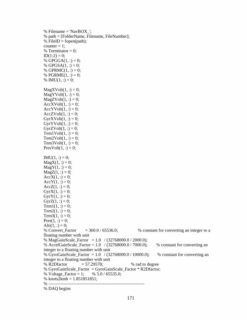
171

% Filename = 'NavBOX_'; % path = [FolderName, Filename, FileNumber]; % FileID = fopen(path); counter = 1; % Terminator = 0; ID(1:2) = 0; % GPGGA(1, :) = 0; % GPGSA(1, :) = 0; % GPRMC(1, :) = 0; % PGRME(1, :) = 0; % IMU(1, :) = 0; MagXVolt(1, :) = 0; MagYVolt(1, :) = 0; MagZVolt(1, :) = 0; AccXVolt(1, :) = 0; AccYVolt(1, :) = 0; AccZVolt(1, :) = 0; GyrXVolt(1, :) = 0; GyrYVolt(1, :) = 0; GyrZVolt(1, :) = 0; Tem1Volt(1, :) = 0; Tem2Volt(1, :) = 0; Tem3Volt(1, :) = 0; PresVolt(1, :) = 0; IMU(1, :) = 0; MagX(1, :) = 0; MagY(1, :) = 0; MagZ(1, :) = 0; AccX(1, :) = 0; AccY(1, :) = 0; AccZ(1, :) = 0; GyrX(1, :) = 0; GyrY(1, :) = 0; GyrZ(1, :) = 0; Tem1(1, :) = 0; Tem2(1, :) = 0; Tem3(1, :) = 0; Pres(1, :) = 0; Alti(1, :) = 0; % Convert_Factor = 360.0 / 65536.0; % constant for converting an integer to a floating number with unit % MagGainScale_Factor = 1.0 / (32768000.0 / 2000.0); % AccelGainScale_Factor = 1.0 / (32768000.0 / 7000.0); % constant for converting an integer to a floating number with unit % GyroGainScale_Factor = 1.0 / (32768000.0 / 10000.0); % constant for converting an integer to a floating number with unit % R2Dfactor = 57.29578; % rad to degree % GyroGainScale_Factor = GyroGainScale_Factor * R2Dfactor; % Voltage_Factor = 1; % 5.0 / 65535.0; % knots2kmh = 1.851851851; % ----------------------------------------------------------------- % DAQ begins

172

% ----------------------------------------------------------------- tic % ===================================================================== %initialize the flag variable set(handles.Start,'UserData',1); Aff = 0; %while the flag variable is one, the loop continues while (get(handles.Start,'UserData') ==1) % ===================================================================== if (ID(1) == 170) && (ID(2) == 170) IMU(counter, 1:26) = fread(SP, 26, 'uchar'); IMU(counter, 27) = fread(SP, 1, 'uint32'); % if counter == 4 % kkkk = 1; % end MagXVolt(counter) = ((IMU(counter, 1) * 256 + IMU(counter, 2)) / 65535) * 5.002; MagYVolt(counter) = ((IMU(counter, 3) * 256 + IMU(counter, 4)) / 65535) * 5.002; MagZVolt(counter) = ((IMU(counter, 5) * 256 + IMU(counter, 6)) / 65535) * 5.002; AccXVolt(counter) = ((IMU(counter, 7) * 256 + IMU(counter, 8)) / 65535) * 5.002; AccYVolt(counter) = ((IMU(counter, 9) * 256 + IMU(counter, 10)) / 65535) * 5.002; AccZVolt(counter) = ((IMU(counter, 11) * 256 + IMU(counter, 12)) / 65535) * 5.002; GyrXVolt(counter) = ((IMU(counter, 13) * 256 + IMU(counter, 14)) / 65535) * 5.002; GyrYVolt(counter) = ((IMU(counter, 15) * 256 + IMU(counter, 16)) / 65535) * 5.002; GyrZVolt(counter) = ((IMU(counter, 17) * 256 + IMU(counter, 18)) / 65535) * 5.002; Tem1Volt(counter) = ((IMU(counter, 19) * 256 + IMU(counter, 20)) / 65535) * 5.002; Tem2Volt(counter) = ((IMU(counter, 21) * 256 + IMU(counter, 22)) / 65535) * 5.002; Tem3Volt(counter) = ((IMU(counter, 23) * 256 + IMU(counter, 24)) / 65535) * 5.002; PresVolt(counter) = ((IMU(counter, 25) * 256 + IMU(counter, 26)) / 65535) * 5.002; MagX(counter) = -1.11594593180632 * MagXVolt(counter) + 2.754143684390910; MagY(counter) = -1.10279951197394 * MagYVolt(counter) + 2.493201861604370; MagZ(counter) = 3.115863255903920 * MagZVolt(counter) - 9.36259619042738; AccX(counter) = 0.714285714285714 * AccXVolt(counter) - 1.78571428571429; AccY(counter) = -0.714285714285714 * AccYVolt(counter) + 1.78571428571429; AccZ(counter) = 0.714285714285714 * AccZVolt(counter) - 1.78571428571429; GyrX(counter) = ((GyrXVolt(counter) - 2.46020) * 1000) / 12.5; GyrY(counter) = ((GyrYVolt(counter) - 2.49898) * 1000) / 12.5; GyrZ(counter) = ((GyrZVolt(counter) - 2.62720) * 1000) / 12.5; Tem1(counter) = Tem1Volt(counter) * 110 - 250; Tem2(counter) = Tem2Volt(counter) * 110 - 250; Tem3(counter) = Tem3Volt(counter) * 110 - 250; Pres(counter) = (PresVolt(counter)/5.002 + 0.152)/0.01059; Alti(counter) = ((1 - (Pres(counter)/100.325)^0.19026) * 288.15) / 0.00198122; pitch = atand((AccX(counter) - 0)/(AccZ(counter) - 0)); roll = atand((0 - AccY(counter))/(AccZ(counter) - 0)); MagXH = (MagX(counter)-0)*cosd(pitch) + (MagY(counter)-0) * sind(pitch) * sind(roll) - (MagZ(counter)-0)*cosd(roll)*sind(pitch); MagYH = (MagY(counter)-0)*cosd(roll) + (MagZ(counter)-0) * sind(roll);

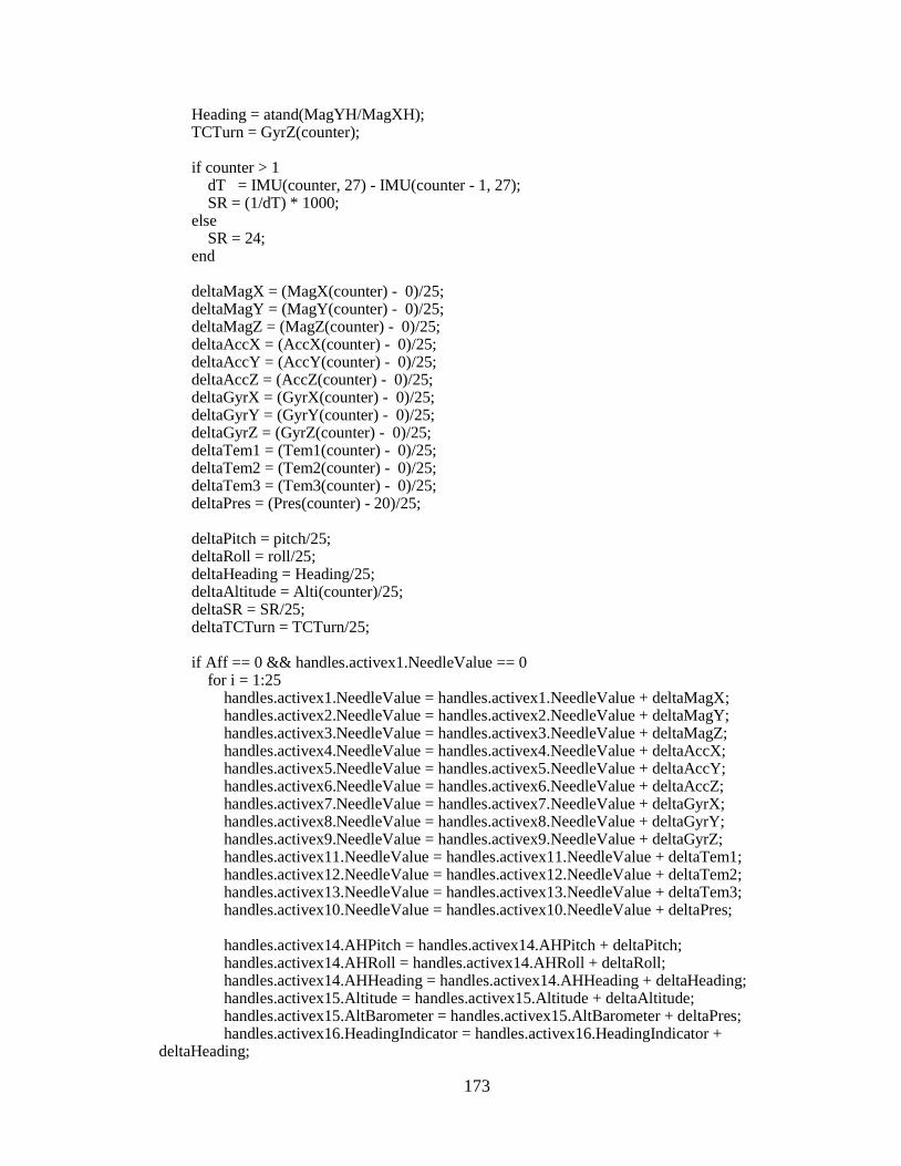
173

Heading = atand(MagYH/MagXH); TCTurn = GyrZ(counter); if counter > 1 dT = IMU(counter, 27) - IMU(counter - 1, 27); SR = (1/dT) * 1000; else SR = 24; end deltaMagX = (MagX(counter) - 0)/25; deltaMagY = (MagY(counter) - 0)/25; deltaMagZ = (MagZ(counter) - 0)/25; deltaAccX = (AccX(counter) - 0)/25; deltaAccY = (AccY(counter) - 0)/25; deltaAccZ = (AccZ(counter) - 0)/25; deltaGyrX = (GyrX(counter) - 0)/25; deltaGyrY = (GyrY(counter) - 0)/25; deltaGyrZ = (GyrZ(counter) - 0)/25; deltaTem1 = (Tem1(counter) - 0)/25; deltaTem2 = (Tem2(counter) - 0)/25; deltaTem3 = (Tem3(counter) - 0)/25; deltaPres = (Pres(counter) - 20)/25; deltaPitch = pitch/25; deltaRoll = roll/25; deltaHeading = Heading/25; deltaAltitude = Alti(counter)/25; deltaSR = SR/25; deltaTCTurn = TCTurn/25; if Aff == 0 && handles.activex1.NeedleValue == 0 for i = 1:25 handles.activex1.NeedleValue = handles.activex1.NeedleValue + deltaMagX; handles.activex2.NeedleValue = handles.activex2.NeedleValue + deltaMagY; handles.activex3.NeedleValue = handles.activex3.NeedleValue + deltaMagZ; handles.activex4.NeedleValue = handles.activex4.NeedleValue + deltaAccX; handles.activex5.NeedleValue = handles.activex5.NeedleValue + deltaAccY; handles.activex6.NeedleValue = handles.activex6.NeedleValue + deltaAccZ; handles.activex7.NeedleValue = handles.activex7.NeedleValue + deltaGyrX; handles.activex8.NeedleValue = handles.activex8.NeedleValue + deltaGyrY; handles.activex9.NeedleValue = handles.activex9.NeedleValue + deltaGyrZ; handles.activex11.NeedleValue = handles.activex11.NeedleValue + deltaTem1; handles.activex12.NeedleValue = handles.activex12.NeedleValue + deltaTem2; handles.activex13.NeedleValue = handles.activex13.NeedleValue + deltaTem3; handles.activex10.NeedleValue = handles.activex10.NeedleValue + deltaPres; handles.activex14.AHPitch = handles.activex14.AHPitch + deltaPitch; handles.activex14.AHRoll = handles.activex14.AHRoll + deltaRoll; handles.activex14.AHHeading = handles.activex14.AHHeading + deltaHeading; handles.activex15.Altitude = handles.activex15.Altitude + deltaAltitude; handles.activex15.AltBarometer = handles.activex15.AltBarometer + deltaPres; handles.activex16.HeadingIndicator = handles.activex16.HeadingIndicator + deltaHeading;

174

handles.activex18.TCTurn = handles.activex18.TCTurn + deltaTCTurn; handles.activex18.TCInclinometer = handles.activex18.TCInclinometer + deltaRoll; handles.activex20.Airspeed = handles.activex20.Airspeed + deltaSR; set(handles.edit1, 'String', num2str(MagXVolt(counter), '%.5f')); set(handles.edit2, 'String', num2str(MagYVolt(counter), '%.5f')); set(handles.edit3, 'String', num2str(MagZVolt(counter), '%.5f')); set(handles.edit4, 'String', num2str(AccXVolt(counter), '%.5f')); set(handles.edit5, 'String', num2str(AccYVolt(counter), '%.5f')); set(handles.edit6, 'String', num2str(AccZVolt(counter), '%.5f')); set(handles.edit7, 'String', num2str(GyrXVolt(counter), '%.5f')); set(handles.edit8, 'String', num2str(GyrYVolt(counter), '%.5f')); set(handles.edit9, 'String', num2str(GyrZVolt(counter), '%.5f')); set(handles.edit11, 'String', num2str(Tem1Volt(counter), '%.5f')); set(handles.edit12, 'String', num2str(Tem2Volt(counter), '%.5f')); set(handles.edit13, 'String', num2str(Tem3Volt(counter), '%.5f')); set(handles.edit10, 'String', num2str(PresVolt(counter), '%.5f')); for j = 1:3000000 end drawnow end Aff = 1; else if counter > 10 handles.activex1.NeedleValue = sum(MagX(1,counter-9:counter))/10; handles.activex2.NeedleValue = sum(MagY(1,counter-9:counter))/10; handles.activex3.NeedleValue = sum(MagZ(1,counter-9:counter))/10; handles.activex4.NeedleValue = sum(AccX(1,counter-9:counter))/10; handles.activex5.NeedleValue = sum(AccY(1,counter-9:counter))/10; handles.activex6.NeedleValue = sum(AccZ(1,counter-9:counter))/10; handles.activex7.NeedleValue = sum(GyrX(1,counter-9:counter))/10; handles.activex8.NeedleValue = sum(GyrY(1,counter-9:counter))/10; handles.activex9.NeedleValue = sum(GyrZ(1,counter-9:counter))/10; handles.activex11.NeedleValue = sum(Tem1(1,counter-9:counter))/10; handles.activex12.NeedleValue = sum(Tem2(1,counter-9:counter))/10; handles.activex13.NeedleValue = sum(Tem3(1,counter-9:counter))/10; handles.activex10.NeedleValue = sum(Pres(1,counter-9:counter))/10; pitch = atand(((-sum(AccX(1,counter-9:counter))/10))/((sum(AccZ(1,counter-9:counter))/10))); roll = atand((0 - (sum(AccY(1,counter-9:counter))/10))/((sum(AccZ(1,counter-9:counter))/10) - 0)); MagXH = ((sum(MagX(1,counter-9:counter))/10)-0)*cosd(pitch) + ((sum(MagY(1,counter-9:counter))/10)-0)*sind(pitch)*sind(roll) - ((sum(MagZ(1,counter-9:counter))/10)-0)*cosd(roll)*sind(pitch); MagYH = ((sum(MagY(1,counter-9:counter))/10)-0)*cosd(roll) + ((sum(MagZ(1,counter-9:counter))/10)-0)*sind(roll); handles.activex14.AHPitch = pitch; handles.activex14.AHRoll = roll; handles.activex14.AHHeading = atand(MagYH/MagXH); handles.activex15.Altitude = sum(Alti(1,counter-9:counter))/10;

175

handles.activex15.AltBarometer = sum(Pres(1,counter-9:counter))/10; handles.activex16.HeadingIndicator = atand(MagYH/MagXH); handles.activex18.TCTurn = sum(GyrZ(1,counter-9:counter))/10; handles.activex18.TCInclinometer = roll; handles.activex20.Airspeed = SR; set(handles.edit1, 'String', num2str(MagXVolt(counter), '%.5f')); set(handles.edit2, 'String', num2str(MagYVolt(counter), '%.5f')); set(handles.edit3, 'String', num2str(MagZVolt(counter), '%.5f')); set(handles.edit4, 'String', num2str(AccXVolt(counter), '%.5f')); set(handles.edit5, 'String', num2str(AccYVolt(counter), '%.5f')); set(handles.edit6, 'String', num2str(AccZVolt(counter), '%.5f')); set(handles.edit7, 'String', num2str(GyrXVolt(counter), '%.5f')); set(handles.edit8, 'String', num2str(GyrYVolt(counter), '%.5f')); set(handles.edit9, 'String', num2str(GyrZVolt(counter), '%.5f')); set(handles.edit11, 'String', num2str(Tem1Volt(counter), '%.5f')); set(handles.edit12, 'String', num2str(Tem2Volt(counter), '%.5f')); set(handles.edit13, 'String', num2str(Tem3Volt(counter), '%.5f')); set(handles.edit10, 'String', num2str(PresVolt(counter), '%.5f')); set(handles.edit14, 'String', num2str(SR, '%.5f')); else handles.activex1.NeedleValue = MagX(counter); handles.activex2.NeedleValue = MagY(counter); handles.activex3.NeedleValue = MagZ(counter); handles.activex4.NeedleValue = AccX(counter); handles.activex5.NeedleValue = AccY(counter); handles.activex6.NeedleValue = AccZ(counter); handles.activex7.NeedleValue = GyrX(counter); handles.activex8.NeedleValue = GyrY(counter); handles.activex9.NeedleValue = GyrZ(counter); handles.activex11.NeedleValue = Tem1(counter); handles.activex12.NeedleValue = Tem2(counter); handles.activex13.NeedleValue = Tem3(counter); handles.activex10.NeedleValue = Pres(counter); pitch = atand((AccX(counter) - 0)/(AccZ(counter) - 0)); roll = atand((0 - AccY(counter))/(AccZ(counter) - 0)); MagXH = (MagX(counter)-0)*cosd(pitch) + (MagY(counter)-0)*sind(pitch)*sind(roll) - (MagZ(counter)-0)*cosd(roll)*sind(pitch); MagYH = (MagY(counter)-0)*cosd(roll) + (MagZ(counter)-0)*sind(roll); handles.activex14.AHPitch = pitch; handles.activex14.AHRoll = roll; handles.activex14.AHHeading = atand(MagYH/MagXH); handles.activex15.Altitude = Alti(counter); handles.activex15.AltBarometer = Pres(counter); handles.activex16.HeadingIndicator = atand(MagYH/MagXH); handles.activex18.TCTurn = GyrZ(counter); handles.activex18.TCInclinometer = roll; handles.activex20.Airspeed = SR;

176

set(handles.edit1, 'String', num2str(MagXVolt(counter), '%.5f')); set(handles.edit2, 'String', num2str(MagYVolt(counter), '%.5f')); set(handles.edit3, 'String', num2str(MagZVolt(counter), '%.5f')); set(handles.edit4, 'String', num2str(AccXVolt(counter), '%.5f')); set(handles.edit5, 'String', num2str(AccYVolt(counter), '%.5f')); set(handles.edit6, 'String', num2str(AccZVolt(counter), '%.5f')); set(handles.edit7, 'String', num2str(GyrXVolt(counter), '%.5f')); set(handles.edit8, 'String', num2str(GyrYVolt(counter), '%.5f')); set(handles.edit9, 'String', num2str(GyrZVolt(counter), '%.5f')); set(handles.edit11, 'String', num2str(Tem1Volt(counter), '%.5f')); set(handles.edit12, 'String', num2str(Tem2Volt(counter), '%.5f')); set(handles.edit13, 'String', num2str(Tem3Volt(counter), '%.5f')); set(handles.edit10, 'String', num2str(PresVolt(counter), '%.5f')); set(handles.edit14, 'String', num2str(SR, '%.5f')); end end counter = counter + 1; % set(SP, 'ByteOrder', 'bigEndian'); % set(SP, 'ByteOrder', 'littleEndian'); % IMU(counter(5), 1:3) = fread(SP, 3, 'int16'); % IMU(counter(5), 4:6) = fread(SP, 3, 'int16'); % IMU(counter(5), 7:9) = fread(SP, 3, 'int16'); % IMU(counter(5), 10) = fread(SP, 1, 'int16'); % DiscardChecksum = fread(SP, 1, 'uint16'); % set(SP, 'ByteOrder', 'littleEndian'); % IMU(counter(5), 11) = fread(SP, 1, 'uint32'); % counter(5) = counter(5) + 1; ID = fread(SP, 2, 'uchar'); % dispcounter = dispcounter + 1; % disp() will slow down the program % if dispcounter >= 21 %#ok<ALIGN,ALIGN> % so display the data every 250 entries % disp([num2str(counter(5) - 1), ' ', ... % num2str(IMU(counter(5) - 1, 1)), ' ', ... % num2str(IMU(counter(5) - 1, 2)), ' ', ... % num2str(IMU(counter(5) - 1, 3)), ' ', ... % num2str(IMU(counter(5) - 1, 10)), ' ', ... % num2str(IMU(counter(5) - 1, 11))]); % display the acceleration data % dispcounter = 1; % reset counter % end else ID = fread(SP, 2, 'uchar'); end % ===================================================================== % handles.activex1.NeedleValue = 2.5; drawnow end Aff = 0; t = toc; disp('Receiving Complete!'); disp(['Serial port communication took ', num2str(t), ' seconds']); fclose(SP); % disconnect serial port object from device

177

delete(SP); % remove serial port object from memory clear SP; % remove serial port object from MATLAB workspace guidata(hObject, handles); % --- Executes on button press in Stop. function Stop_Callback(hObject, eventdata, handles) % hObject handle to Stop (see GCBO) % eventdata reserved - to be defined in a future version of MATLAB % handles structure with handles and user data (see GUIDATA) %toggle the flag variable so that the other process will stop set(handles.Start,'UserData',0); guidata(hObject, handles); function edit1_Callback(hObject, eventdata, handles) % hObject handle to edit1 (see GCBO) % eventdata reserved - to be defined in a future version of MATLAB % handles structure with handles and user data (see GUIDATA) % Hints: get(hObject,'String') returns contents of edit1 as text % str2double(get(hObject,'String')) returns contents of edit1 as a double % --- Executes during object creation, after setting all properties. function edit1_CreateFcn(hObject, eventdata, handles) % hObject handle to edit1 (see GCBO) % eventdata reserved - to be defined in a future version of MATLAB % handles empty - handles not created until after all CreateFcns called % Hint: edit controls usually have a white background on Windows. % See ISPC and COMPUTER. set(hObject, 'String', '0.00000'); if ispc && isequal(get(hObject,'BackgroundColor'), get(0,'defaultUicontrolBackgroundColor')) set(hObject,'BackgroundColor','white'); end function edit11_Callback(hObject, eventdata, handles) % hObject handle to edit11 (see GCBO) % eventdata reserved - to be defined in a future version of MATLAB % handles structure with handles and user data (see GUIDATA) % Hints: get(hObject,'String') returns contents of edit11 as text % str2double(get(hObject,'String')) returns contents of edit11 as a double % --- Executes during object creation, after setting all properties. function edit11_CreateFcn(hObject, eventdata, handles) % hObject handle to edit11 (see GCBO) % eventdata reserved - to be defined in a future version of MATLAB % handles empty - handles not created until after all CreateFcns called % Hint: edit controls usually have a white background on Windows.

178

% See ISPC and COMPUTER. set(hObject, 'String', '0.00000'); if ispc && isequal(get(hObject,'BackgroundColor'), get(0,'defaultUicontrolBackgroundColor')) set(hObject,'BackgroundColor','white'); end function edit12_Callback(hObject, eventdata, handles) % hObject handle to edit12 (see GCBO) % eventdata reserved - to be defined in a future version of MATLAB % handles structure with handles and user data (see GUIDATA) % Hints: get(hObject,'String') returns contents of edit12 as text % str2double(get(hObject,'String')) returns contents of edit12 as a double % --- Executes during object creation, after setting all properties. function edit12_CreateFcn(hObject, eventdata, handles) % hObject handle to edit12 (see GCBO) % eventdata reserved - to be defined in a future version of MATLAB % handles empty - handles not created until after all CreateFcns called % Hint: edit controls usually have a white background on Windows. % See ISPC and COMPUTER. set(hObject, 'String', '0.00000'); if ispc && isequal(get(hObject,'BackgroundColor'), get(0,'defaultUicontrolBackgroundColor')) set(hObject,'BackgroundColor','white'); end function edit13_Callback(hObject, eventdata, handles) % hObject handle to edit13 (see GCBO) % eventdata reserved - to be defined in a future version of MATLAB % handles structure with handles and user data (see GUIDATA) % Hints: get(hObject,'String') returns contents of edit13 as text % str2double(get(hObject,'String')) returns contents of edit13 as a double % --- Executes during object creation, after setting all properties. function edit13_CreateFcn(hObject, eventdata, handles) % hObject handle to edit13 (see GCBO) % eventdata reserved - to be defined in a future version of MATLAB % handles empty - handles not created until after all CreateFcns called % Hint: edit controls usually have a white background on Windows. % See ISPC and COMPUTER. set(hObject, 'String', '0.00000'); if ispc && isequal(get(hObject,'BackgroundColor'), get(0,'defaultUicontrolBackgroundColor')) set(hObject,'BackgroundColor','white'); end

179

function edit10_Callback(hObject, eventdata, handles) % hObject handle to edit10 (see GCBO) % eventdata reserved - to be defined in a future version of MATLAB % handles structure with handles and user data (see GUIDATA) % Hints: get(hObject,'String') returns contents of edit10 as text % str2double(get(hObject,'String')) returns contents of edit10 as a double % --- Executes during object creation, after setting all properties. function edit10_CreateFcn(hObject, eventdata, handles) % hObject handle to edit10 (see GCBO) % eventdata reserved - to be defined in a future version of MATLAB % handles empty - handles not created until after all CreateFcns called % Hint: edit controls usually have a white background on Windows. % See ISPC and COMPUTER. set(hObject, 'String', '0.00000'); if ispc && isequal(get(hObject,'BackgroundColor'), get(0,'defaultUicontrolBackgroundColor')) set(hObject,'BackgroundColor','white'); end function edit7_Callback(hObject, eventdata, handles) % hObject handle to edit7 (see GCBO) % eventdata reserved - to be defined in a future version of MATLAB % handles structure with handles and user data (see GUIDATA) % Hints: get(hObject,'String') returns contents of edit7 as text % str2double(get(hObject,'String')) returns contents of edit7 as a double % --- Executes during object creation, after setting all properties. function edit7_CreateFcn(hObject, eventdata, handles) % hObject handle to edit7 (see GCBO) % eventdata reserved - to be defined in a future version of MATLAB % handles empty - handles not created until after all CreateFcns called % Hint: edit controls usually have a white background on Windows. % See ISPC and COMPUTER. set(hObject, 'String', '0.00000'); if ispc && isequal(get(hObject,'BackgroundColor'), get(0,'defaultUicontrolBackgroundColor')) set(hObject,'BackgroundColor','white'); end function edit8_Callback(hObject, eventdata, handles) % hObject handle to edit8 (see GCBO) % eventdata reserved - to be defined in a future version of MATLAB % handles structure with handles and user data (see GUIDATA)

180

% Hints: get(hObject,'String') returns contents of edit8 as text % str2double(get(hObject,'String')) returns contents of edit8 as a double % --- Executes during object creation, after setting all properties. function edit8_CreateFcn(hObject, eventdata, handles) % hObject handle to edit8 (see GCBO) % eventdata reserved - to be defined in a future version of MATLAB % handles empty - handles not created until after all CreateFcns called % Hint: edit controls usually have a white background on Windows. % See ISPC and COMPUTER. set(hObject, 'String', '0.00000'); if ispc && isequal(get(hObject,'BackgroundColor'), get(0,'defaultUicontrolBackgroundColor')) set(hObject,'BackgroundColor','white'); end function edit9_Callback(hObject, eventdata, handles) % hObject handle to edit9 (see GCBO) % eventdata reserved - to be defined in a future version of MATLAB % handles structure with handles and user data (see GUIDATA) % Hints: get(hObject,'String') returns contents of edit9 as text % str2double(get(hObject,'String')) returns contents of edit9 as a double % --- Executes during object creation, after setting all properties. function edit9_CreateFcn(hObject, eventdata, handles) % hObject handle to edit9 (see GCBO) % eventdata reserved - to be defined in a future version of MATLAB % handles empty - handles not created until after all CreateFcns called % Hint: edit controls usually have a white background on Windows. % See ISPC and COMPUTER. set(hObject, 'String', '0.00000'); if ispc && isequal(get(hObject,'BackgroundColor'), get(0,'defaultUicontrolBackgroundColor')) set(hObject,'BackgroundColor','white'); end function edit4_Callback(hObject, eventdata, handles) % hObject handle to edit4 (see GCBO) % eventdata reserved - to be defined in a future version of MATLAB % handles structure with handles and user data (see GUIDATA) % Hints: get(hObject,'String') returns contents of edit4 as text % str2double(get(hObject,'String')) returns contents of edit4 as a double % --- Executes during object creation, after setting all properties.

181

function edit4_CreateFcn(hObject, eventdata, handles) % hObject handle to edit4 (see GCBO) % eventdata reserved - to be defined in a future version of MATLAB % handles empty - handles not created until after all CreateFcns called % Hint: edit controls usually have a white background on Windows. % See ISPC and COMPUTER. set(hObject, 'String', '0.00000'); if ispc && isequal(get(hObject,'BackgroundColor'), get(0,'defaultUicontrolBackgroundColor')) set(hObject,'BackgroundColor','white'); end function edit5_Callback(hObject, eventdata, handles) % hObject handle to edit5 (see GCBO) % eventdata reserved - to be defined in a future version of MATLAB % handles structure with handles and user data (see GUIDATA) % Hints: get(hObject,'String') returns contents of edit5 as text % str2double(get(hObject,'String')) returns contents of edit5 as a double % --- Executes during object creation, after setting all properties. function edit5_CreateFcn(hObject, eventdata, handles) % hObject handle to edit5 (see GCBO) % eventdata reserved - to be defined in a future version of MATLAB % handles empty - handles not created until after all CreateFcns called % Hint: edit controls usually have a white background on Windows. % See ISPC and COMPUTER. set(hObject, 'String', '0.00000'); if ispc && isequal(get(hObject,'BackgroundColor'), get(0,'defaultUicontrolBackgroundColor')) set(hObject,'BackgroundColor','white'); end function edit6_Callback(hObject, eventdata, handles) % hObject handle to edit6 (see GCBO) % eventdata reserved - to be defined in a future version of MATLAB % handles structure with handles and user data (see GUIDATA) % Hints: get(hObject,'String') returns contents of edit6 as text % str2double(get(hObject,'String')) returns contents of edit6 as a double % --- Executes during object creation, after setting all properties. function edit6_CreateFcn(hObject, eventdata, handles) % hObject handle to edit6 (see GCBO) % eventdata reserved - to be defined in a future version of MATLAB % handles empty - handles not created until after all CreateFcns called % Hint: edit controls usually have a white background on Windows.

182

% See ISPC and COMPUTER. set(hObject, 'String', '0.00000'); if ispc && isequal(get(hObject,'BackgroundColor'), get(0,'defaultUicontrolBackgroundColor')) set(hObject,'BackgroundColor','white'); end function edit2_Callback(hObject, eventdata, handles) % hObject handle to edit2 (see GCBO) % eventdata reserved - to be defined in a future version of MATLAB % handles structure with handles and user data (see GUIDATA) % Hints: get(hObject,'String') returns contents of edit2 as text % str2double(get(hObject,'String')) returns contents of edit2 as a double % --- Executes during object creation, after setting all properties. function edit2_CreateFcn(hObject, eventdata, handles) % hObject handle to edit2 (see GCBO) % eventdata reserved - to be defined in a future version of MATLAB % handles empty - handles not created until after all CreateFcns called % Hint: edit controls usually have a white background on Windows. % See ISPC and COMPUTER. set(hObject, 'String', '0.00000'); if ispc && isequal(get(hObject,'BackgroundColor'), get(0,'defaultUicontrolBackgroundColor')) set(hObject,'BackgroundColor','white'); end function edit3_Callback(hObject, eventdata, handles) % hObject handle to edit3 (see GCBO) % eventdata reserved - to be defined in a future version of MATLAB % handles structure with handles and user data (see GUIDATA) % Hints: get(hObject,'String') returns contents of edit3 as text % str2double(get(hObject,'String')) returns contents of edit3 as a double % --- Executes during object creation, after setting all properties. function edit3_CreateFcn(hObject, eventdata, handles) % hObject handle to edit3 (see GCBO) % eventdata reserved - to be defined in a future version of MATLAB % handles empty - handles not created until after all CreateFcns called % Hint: edit controls usually have a white background on Windows. % See ISPC and COMPUTER. set(hObject, 'String', '0.00000'); if ispc && isequal(get(hObject,'BackgroundColor'), get(0,'defaultUicontrolBackgroundColor')) set(hObject,'BackgroundColor','white'); end

183

function edit14_Callback(hObject, eventdata, handles) % hObject handle to edit14 (see GCBO) % eventdata reserved - to be defined in a future version of MATLAB % handles structure with handles and user data (see GUIDATA) % Hints: get(hObject,'String') returns contents of edit14 as text % str2double(get(hObject,'String')) returns contents of edit14 as a double % --- Executes during object creation, after setting all properties. function edit14_CreateFcn(hObject, eventdata, handles) % hObject handle to edit14 (see GCBO) % eventdata reserved - to be defined in a future version of MATLAB % handles empty - handles not created until after all CreateFcns called % Hint: edit controls usually have a white background on Windows. % See ISPC and COMPUTER. if ispc && isequal(get(hObject,'BackgroundColor'), get(0,'defaultUicontrolBackgroundColor')) set(hObject,'BackgroundColor','white'); end % --- Executes on button press in About. function About_Callback(hObject, eventdata, handles) % hObject handle to About (see GCBO) % eventdata reserved - to be defined in a future version of MATLAB % handles structure with handles and user data (see GUIDATA) % --- Executes on button press in Save. function Save_Callback(hObject, eventdata, handles) % hObject handle to Save (see GCBO) % eventdata reserved - to be defined in a future version of MATLAB % handles structure with handles and user data (see GUIDATA) % --- Executes on button press in Reset. function Reset_Callback(hObject, eventdata, handles) % hObject handle to Reset (see GCBO) % eventdata reserved - to be defined in a future version of MATLAB % handles structure with handles and user data (see GUIDATA) handles.activex1.NeedleValue = 0; handles.activex2.NeedleValue = 0; handles.activex3.NeedleValue = 0; handles.activex4.NeedleValue = 0; handles.activex5.NeedleValue = 0; handles.activex6.NeedleValue = 0; handles.activex7.NeedleValue = 0; handles.activex8.NeedleValue = 0; handles.activex9.NeedleValue = 0; handles.activex11.NeedleValue = 0; handles.activex12.NeedleValue = 0;

184

handles.activex13.NeedleValue = 0; handles.activex10.NeedleValue = 20; handles.activex14.AHPitch = 0; handles.activex14.AHRoll = 0; handles.activex14.AHHeading = 0; handles.activex15.Altitude = 0; handles.activex16.HeadingIndicator = 0; handles.activex18.TCTurn = 0; handles.activex18.TCInclinometer = 0; handles.activex20.Airspeed = 0; set(handles.edit1, 'String', num2str(0, '%.5f')); set(handles.edit2, 'String', num2str(0, '%.5f')); set(handles.edit3, 'String', num2str(0, '%.5f')); set(handles.edit4, 'String', num2str(0, '%.5f')); set(handles.edit5, 'String', num2str(0, '%.5f')); set(handles.edit6, 'String', num2str(0, '%.5f')); set(handles.edit7, 'String', num2str(0, '%.5f')); set(handles.edit8, 'String', num2str(0, '%.5f')); set(handles.edit9, 'String', num2str(0, '%.5f')); set(handles.edit11, 'String', num2str(0, '%.5f')); set(handles.edit12, 'String', num2str(0, '%.5f')); set(handles.edit13, 'String', num2str(0, '%.5f')); set(handles.edit10, 'String', num2str(0, '%.5f'));

185

ProcessFA.m

% function [??? tr] = ProcessFA(Folder) isfunct = 0; % ------------------------------------------------------------------------- % This matlab program is designed to calculate the displacement based % on x-axis acceleration (the sensor is attached to a walking person's foot) % The 'FA' in file name is short for 'Foot Attached IMU' % file name: ProcessFA.m % last revise: 11/04/2008 % ------------------------------------------------------------------------- if isfunct == 0 clear; % clear workspace clc; % clear command window isfunct = 0; end % ------------------------------------------------------------------------- % 0. locate the folder in which the file locates % ------------------------------------------------------------------------- if isfunct == 0 Folder = 'D:\Research & Projects\Navigation\PNS Project\Data\Foot Attached IMU\'; end % ------------------------------------------------------------------------- % 1. Load data into workspace (check data corruption and reconstruction) % ------------------------------------------------------------------------- FileName = '10-02-2008-t1943.txt'; % 96.18 m walking - constant speed % FileName = '10-02-2008-t1948.txt'; % 96.18 m walking - constant speed % FileName = '10-02-2008-t1950.txt'; % 96.18 m walking - var speed % FileName = '10-02-2008-t1952.txt'; % 96.18 m walking/running % FileName = '10-02-2008-t1954.txt'; % 96.18 m walking - constant speed % FileName = '10-02-2008-t1956.txt'; % stairs % FileName = '10-02-2008-t1958.txt'; % stairs % FileName = '11-12-2008-t1618.txt'; % const spd % FileName = '11-12-2008-t1620.txt'; % const spd % FileName = '11-12-2008-t1624.txt'; % const spd % FileName = '11-12-2008-t1626.txt'; % const spd % FileName = '11-12-2008-t1628.txt'; % const spd % FileName = '11-12-2008-t1629.txt'; % const spd % FileName = '11-12-2008-t1631.txt'; % const spd % FileName = '11-12-2008-t1634.txt'; % const spd % FileName = '11-12-2008-t1636.txt'; % const spd % FileName = '11-12-2008-t1652.txt'; % const spd % FileName = '11-12-2008-t1654.txt'; % const spd % FileName = '11-12-2008-t1656.txt'; % const spd % FileName = '11-12-2008-t1707.txt'; % const spd w/ stop % FileName = '11-12-2008-t1709.txt'; % const spd w/ stop % FileName = '11-12-2008-t1711.txt'; % const spd w/ stop % FileName = '11-12-2008-t1714.txt'; % variable spd % FileName = '11-12-2008-t1716.txt'; % variable spd % FileName = '11-12-2008-t1722.txt'; % variable spd % FileName = '11-12-2008-t1724.txt'; % variable spd

186

% FileName = '11-12-2008-t1726.txt'; % variable spd % FileName = '11-12-2008-t1727.txt'; % variable spd % FileName = '11-12-2008-t1730.txt'; % walking/running % FileName = '11-12-2008-t1731.txt'; % walking/running % FileName = '11-12-2008-t1733.txt'; % walking/running % FileName = '11-12-2008-t1734.txt'; % walking/running IMU = LoadData(Folder, FileName); % --------------------------------------------------------------------- % 2. Calculate the DAQ time, generating time vector % --------------------------------------------------------------------- N = size(IMU, 1); r = rem(N, 5); if r ~= 0 IMU(N-r+1:N,:) = []; end N = size(IMU, 1); % --------------------------------------------------------------------- % 3. Calculate the DAQ time, generating time vector % --------------------------------------------------------------------- t(:,1) = 0; for i = 1:size(IMU,1)-1 t(i+1) = t(i) + 0.0065536 * abs(abs(IMU(i,10)) - abs(IMU(i+1,10))); end totaltime = t(i+1); Fs = N/totaltime; % ------------------------------------------------------------------------- % 4. Process % ------------------------------------------------------------------------- % find the food movement time interval n = 3; i = 3; j = 3; Start = 0; Ave(1,:) = [0 1]; Ave(2,:) = [0 2]; IntBE(1,:) = 0; IMU(:,4) = IMU(:,4) * 9.81; % convert IMU(:,4) = IMU(:,4) + abs(sum(IMU(1:100,4))/100); % offset AGp = IMU(1:N,8) .* IMU(1:N,4); AGp = AGp'; figure(1); plot(t, AGp, '-o'); grid on title('Product of Acc X and Gyro Y'); xlabel('Time (sec)'); ylabel('Product of Acc X and Gyro Y'); TH = 3;

187

THs = 3.37; while n <= numel(AGp) - 2 if n == 1353 K = 11111; end if abs(AGp(n)) >= TH && std(AGp(1, n-2:n+2)) > THs Ave(i,1) = 1; if Start == 0 if sum(Ave(1:i,1)) > 0 Start = i; end end if Start ~= 0 && Ave(i-1,1) == 0 IntBE(j,1) = n; j = j + 1; end else if std(AGp(1, n-2:n+2)) < THs Ave(i,1) = 0; if Start ~= 0 && Ave(i-1,1) == 1 IntBE(j-1,2) = n-1; end else Ave(i,1) = 1; if Start == 0 if sum(Ave(1:i,1)) > 0 Start = i; end end if Start ~= 0 && Ave(i-1,1) == 0 IntBE(j,1) = n; j = j + 1; end end end Ave(i,2) = n; i = i + 1; n = n + 1; end Ave(n,:) = [0 n]; Ave(n+1,:) = [0 n+1]; IntBE(1:2,:) = []; steps = size(IntBE, 1) * 2; figure(2); plot(Ave(:,1),'-o'); grid on title('Status'); axis([0 size(Ave,1) -1 5]); % calculates the V V(1:IntBE(1,1)-1) = 0; V(:,1) = 0; k = IntBE(1,1);

188

for j = 1 : size(IntBE,1) V(k) = 0; for i = IntBE(j,1) : IntBE(j,2) V(k+1) = V(k) + 0.5 * (IMU(i,4) + IMU(i+1,4)) * abs(abs(IMU(i,10)) - abs(IMU(i+1,10))) * 0.0065536; k = k + 1; end if j <= size(IntBE,1) - 1 V(IntBE(j,2)+2:IntBE(j+1,1)-1) = 0; k = IntBE(j+1,1)-1; end end V(k+1:size(IMU,1)) = 0; % calculates the D D(:,1) = 0; for j = 1 : numel(V)-1 D(j+1) = D(j) + 0.5 * (abs(V(j)) + abs(V(j+1))) * abs(abs(IMU(j,10)) - abs(IMU(j+1,10))) * 0.0065536; end Distance = D(N); disp(['File name: ', FileName]); disp(['Data sampled: ', num2str(N),' entries ']); disp(['Sampling Rate: ', num2str(Fs),' Hz ']); disp(['Test Time: ', num2str(totaltime),' sec ']); disp(['Walked: ', num2str(steps), ' steps ']); disp(['Distance: ', num2str(Distance, 4), ' meters ']); disp([' ', num2str(Distance * 3.28084), ' feet ']); FIR1vector = fir1(30, 0.056); % FIR1 Filter vector AccXFir1 = filter(FIR1vector, 1, IMU(:,4)); % Using FIR1 Filter figure(3); subplot(3,1,1); plot(t, -IMU(:,4)/9.81,'-o'); hold on % plot(t, AccXFir1/9.81,'-r'); hold on % plot(IntBE(:,1),zeros(1, size(IntBE,1)) + IMU(1,4),'ro','LineWidth', 3, 'MarkerSize', 5); grid on; ylabel('Acceleration (G)'); axis([20 25 -4 6]); subplot(3,1,2); plot(t, -V); grid on ylabel('Velocity (m/s)'); axis([20 25 -1 7]); subplot(3,1,3); plot(t, D); grid on ylabel('Distance (m)'); axis([20 25 4 14]); clear isfunct Folder; figure(4);

189

subplot(2,1,1); plot(t, AGp/9.81, '-o'); grid on xlabel('Time (sec)'); ylabel('Product of X-axis acceleration and Y-axis angular rate'); subplot(2,1,2); plot(t, IMU(:,4)/9.81,'-o'); hold on grid on; xlabel('Time (sec)'); ylabel('X-axis acceleration (G)'); % end

190

ProcessKA.m

% ------------------------------------------------------------------------- % This Matlab program calculates the walking distance based on the % angular displacement of a person's leg (the sensor is attached to % a walking person's knee) % The 'KA' in file name is short for 'Knee Attached IMU' % file name: ProcessKA.m % last revise: 11/16/2008 % ------------------------------------------------------------------------- % ------------------------------------------------------------------------- clc; % clear screen clear; % clear workplace % ------------------------------------------------------------------------- % 1. Load data file % ------------------------------------------------------------------------- % filename = '11-12-2008-t2038.txt'; % const spd % filename = '11-12-2008-t2039.txt'; % const spd % filename = '11-12-2008-t2041.txt'; % const spd % filename = '11-12-2008-t2043.txt'; % const spd % filename = '11-12-2008-t2045.txt'; % const spd % filename = '11-12-2008-t2046.txt'; % const spd % filename = '11-12-2008-t2048.txt'; % const spd % filename = '11-12-2008-t2050.txt'; % const spd % filename = '11-12-2008-t2052.txt'; % const spd % filename = '11-12-2008-t2053.txt'; % const spd % filename = '11-12-2008-t2056.txt'; % variable spd % filename = '11-12-2008-t2057.txt'; % variable spd % filename = '11-12-2008-t2058.txt'; % variable spd % filename = '11-12-2008-t2100.txt'; % variable spd % filename = '11-12-2008-t2102.txt'; % walking/running % filename = '11-12-2008-t2103.txt'; % walking/running % filename = '11-12-2008-t2104.txt'; % walking/running % filename = '11-13-2008-t1835.txt'; % const spd w/ stop % filename = '11-13-2008-t1837.txt'; % const spd w/ stop % filename = '11-13-2008-t1839.txt'; % const spd w/ stop % filename = '11-13-2008-t1841.txt'; % walking/running filename = '11-13-2008-t1843.txt'; % stairs - up % filename = '11-13-2008-t1844.txt'; % stairs - down % filename = '11-14-2008-t1915.txt'; % const spd % filename = '11-14-2008-t1917.txt'; % const spd % filename = '11-14-2008-t1918.txt'; % const spd % filename = '11-14-2008-t1920.txt'; % const spd % filename = '11-14-2008-t1922.txt'; % const spd % filename = '11-14-2008-t1923.txt'; % const spd % filename = '11-14-2008-t1925.txt'; % variable spd % filename = '11-14-2008-t1926.txt'; % walking/running % path = ['D:\Research & Projects\Navigation\PNS Project\Data\Knee Attached IMU\T_ID_0x03\', filename]; path = ['D:\Research & Projects\Navigation\PNS Project\Data\Knee Attached IMU\', filename]; IMU = load(path); MagX = IMU(:, 1); % 1st column - x-axis magnetic field

191

MagY = IMU(:, 2); % 2nd column - y-axis magnetic field MagZ = IMU(:, 3); % 1rd column - z-axis magnetic field AccX = IMU(:, 4); % 4th column - x-axis acceleration AccY = IMU(:, 5); % 5th column - y-axis acceleration AccZ = IMU(:, 6); % 6th column - z-axis acceleration GyroX = IMU(:, 7); % 7th column - x-axis angular rate GyroY = IMU(:, 8); % 8th column - y-axis angular rate GyroZ = IMU(:, 9); % 9th column - z-axis angular rate TTs = IMU(:, 10); % 10th column Timer Ticks of Rabbit SUM = IMU(:, 11); % 11th column checksum % ----------------------------------------------------------------- % 2. Data preprocess % ----------------------------------------------------------------- % AccZ = AccZ + 1; AGp = GyroY .* AccZ * 9.81; % ----------------------------------------------------------------- % 3. Calculate total time % ----------------------------------------------------------------- N = length(SUM); % Number of data rollover = 0; % times of roll-over ro(:,1) = 0; % roll-over places for j = 1 : N-1 if (TTs(j) - TTs(j+1)) > 1000 rollover = rollover + 1; ro(rollover) = j; end end if rollover == 0 totaltime = (TTs(N) - TTs(1)) * 0.0065536; else totaltime = ((TTs(ro(1)) - TTs(1)) + (TTs(N) - TTs(1 + ro(rollover)))) * 0.0065536 + (rollover - 1) * 429.4967; end Fs = N / (totaltime); % Hz t = 1/Fs:1/Fs:1*N/Fs; % time axis % % ----------------------------------------------------------------- % % 4. Display the acceleration data % % ----------------------------------------------------------------- % figure(1); % subplot(311); % plot(t, AccX); grid on; hold on; % x axis acceleration % axis([0 1*N/Fs (-max(-AccX)-0.05) (max(AccX)+0.05)]); % xlabel('Time(sec)'); % ylabel('x-axis acceleration (G)'); % title('X-axis acceleration (G)'); % % AxFIR1vector = fir1(10, 0.5); % FIR1 Filter vector % AxFir1 = filter(AxFIR1vector, 1, AccX); % Using FIR1 Filter % plot(t, AxFir1, 'r'); % % subplot(312); % plot(t, AccY); grid on; hold on; % y axis acceleration % axis([0 1*N/Fs (-max(-AccY)-0.05) (max(AccY)+0.05)]); % xlabel('Time(sec)');

192

% ylabel('y-axis acceleration (G)'); % title('Y-axis acceleration (G)'); % % AyFIR1vector = fir1(10, 0.5); % FIR1 Filter vector % AyFir1 = filter(AyFIR1vector, 1, AccY); % Using FIR1 Filter % plot(t, AyFir1, 'r'); % % subplot(313); % plot(t, AccZ); grid on; hold on; % z axis acceleration % axis([0 1*N/Fs (-max(-AccZ)-0.05) (max(AccZ)+0.05)]); % xlabel('Time(sec)'); % ylabel('z-axis acceleration (G)'); % title('Z-axis acceleration (G)'); % % AzFIR1vector = fir1(10, 0.1); % FIR1 Filter vector % AzFir1 = filter(AzFIR1vector, 1, AccY); % Using FIR1 Filter % plot(t, AzFir1, 'r'); % % figure(9); % AzF = fft(AccZ, 16384); % PAzF = AzF.* conj(AzF) / 16384; % f = Fs*(0:8192)/16384; % % figure('Name', 'Freq', 'NumberTitle', 'off'); % plot(f, PAzF(1:8193)); % title('Frequency content of y'); % xlabel('frequency (Hz)'); % % ----------------------------------------------------------------- % % 5. Display the mag data % % ----------------------------------------------------------------- % figure(2); % subplot(311); % plot(t, MagX); grid on; % MagX % axis([0 1*N/Fs (-max(-MagX)-0.05) (max(MagX)+0.05)]); % xlabel('Time(sec)'); % title('MagX'); % subplot(312); % plot(t, MagY); grid on; % MagY % axis([0 1*N/Fs (-max(-MagY)-0.05) (max(MagY)+0.05)]); % xlabel('Time(sec)'); % title('MagY'); % subplot(313); % plot(t, MagZ); grid on; % yall % axis([0 1*N/Fs (-max(-MagZ)-0.05) (max(MagZ)+0.05)]); % xlabel('Time(sec)'); % title('MagZ'); % % ----------------------------------------------------------------- % % 6. display the gyroscope data % % ----------------------------------------------------------------- % figure(3); % subplot(311); % plot(t, GyroX); grid on; % x axis angular rate % axis([0 1*N/Fs (-max(-GyroX)-0.05) (max(GyroX)+0.05)]); % xlabel('Time(sec)'); % title('GyroX');

193

% subplot(312); % plot(t, GyroY); grid on; % y axis angular rate % axis([0 1*N/Fs (-max(-GyroY)-0.05) (max(GyroY)+0.05)]); % xlabel('Time(sec)'); % title('GyroY'); % subplot(313); % plot(t, GyroZ); grid on; % z axis angular rate % axis([0 1*N/Fs (-max(-GyroZ)-0.05) (max(GyroZ)+0.05)]); % xlabel('Time(sec)'); % title('GyroZ'); % ------------------------------------------------------------------------- % 7. Distance calculation based on angular movement of legs - ZADU % ------------------------------------------------------------------------- FIR1vector = fir1(44, 0.056); % FIR1 Filter vector GyroYFir1 = filter(FIR1vector, 1, GyroY); % Using FIR1 Filter GyroYFir2 = abs(GyroYFir1); i = 1; while 1 if GyroYFir2(i) > 2.5; % movement begins break; end i = i + 1; end for j = (i - 10) : (numel(GyroYFir2)-1) if GyroYFir2(j) < GyroYFir2(j-1) && GyroYFir2(j) < GyroYFir2(j+1) && GyroYFir2(j) < 11.5 GyroYFir2(j) = 0; end end swing(1:N) = 0; % initialise for k = 1:N-1 % angular rate integration if GyroYFir2(k) == 0 swing(k) = 0; end swing(k + 1)= swing(k) + ... % to get angular displacement 0.5 * (GyroYFir2(k) + GyroYFir2(k + 1)) * (1/Fs); end figure('Name', 'Angular rate & displacement', 'NumberTitle', 'off'); plot(t, GyroY, '-^b', 'LineWidth', 2); % angular rate grid on; hold on; plot(t, GyroYFir2, '-*k', 'LineWidth', 2); % angular rate hold on; plot(t, swing, '-or', 'LineWidth', 2); % angular displacement xlabel('Time(sec)'); ylabel('Y-axis angular rate (Degree/sec) & angular displacement'); title('Y-axis Angular Rate & Angular displacement');

194

legend('Angular rate', 'Angular rate (Filter)', 'Angular displacement'); % PeakNum = 0; % number of peaks in the waveform % Peak(1, :) = 0; % a vector to store each peak value % for j = 1:N % if abs(swing(j)) > 5 % 5 degree will be the smallest displacement % Begin = j; % any displacement smaller than this % break; % will not be considered % end % end % for j = Begin:N-1 % finding the peaks % if ((swing(j) > swing(j+1)) && (swing(j) > swing(j-1)) ... % || (swing(j) < swing(j+1)) && (swing(j) < swing(j-1))) % PeakNum = PeakNum + 1; % Peak(PeakNum) = j; % end % end % % i = 0; % StrideAngle(1, :) = 0; % difference between two peaks % for j = 2:PeakNum % is the StrideAngle % i = i + 1; % if abs(swing(Peak(j)) - swing(Peak(j-1))) > 10 % StrideAngle(i) = abs(swing(Peak(j)) - swing(Peak(j-1))); % end % end pks = findpeaks(swing); i = 1; k = numel(pks); while i <= k if pks(i) < 5 pks(i) = []; else i = i + 1; end k = numel(pks); end StrideAngle = pks; Distance = 0; % calculate distance L = 1.06; % length of my leg (meter) for j = 1:size(StrideAngle, 2) Distance = Distance + L * sqrt(2 * (1 - cosd(StrideAngle(j)))); end % ----------------------------------------------------------------- % 7. Display all the info % ----------------------------------------------------------------- disp(['File name: ', filename]); disp(['Data sampled: ', num2str(N),' entries ']); disp(['Sampling Rate: ', num2str(Fs),' Hz ']); disp(['Test Time: ', num2str(totaltime),' sec ']); disp(['Walked: ', num2str(numel(pks)), ' steps ']);

195

disp(['Distance: ', num2str(Distance, 4), ' meters ']); disp([' ', num2str(Distance * 3.28084), ' feet ']); % ----------------------------------------------------------------- % 10. heading angle based on x-axis angular rata % ----------------------------------------------------------------- FIR1vector = fir1(140, 0.4/Fs); % FIR1 Filter vector GyroXFir1 = filter(FIR1vector, 1, GyroX); % Using FIR1 Filter % GXF = fft(GyroXFir1, 4096); % PGXF = GXF.* conj(GXF) / 4096; % f = 20*(0:2048)/4096; % figure('Name', 'Freq', 'NumberTitle', 'off'); % plot(f, PGXF(1:2049)); % title('Frequency content of y'); % xlabel('frequency (Hz)'); heading(1:N) = 0; % initialise % for k = 1:N % if abs(GyroXFir1(k)) < 10 % GyroXFir1(k) = 0; % end % end for k = 1:N-1 % angular rate integration heading(k + 1)= heading(k) + ... % to get angular displacement 0.5 * (GyroXFir1(k) + GyroXFir1(k + 1)) * (1/Fs); if abs(heading(k + 1) - heading(k)) < 0.2 heading(k + 1) = heading(k); % elseif heading(k + 1) - heading(k) > 0.7 % heading(k + 1) = heading(k + 1) + 0.3; end end figure('Name', 'Heading angle', 'NumberTitle', 'off'); plot(t, -GyroX, '-^b', 'LineWidth', 2); % angular rate grid on; hold on; plot(t, -GyroXFir1, '-or', 'LineWidth', 2); % angular displacement grid on; hold on; plot(t, -heading, '-ok', 'LineWidth', 2); % angular displacement xlabel('Time(sec)'); ylabel('Heading (Degree)'); %axis([0 1*N/Fs -5 5]); title('Heading'); % xlabel('Time(sec)'); % ylabel('X-axis angular rate (Degree/sec) & angular displacement'); % title('X-axis Angular Rate & Angular displacement'); legend('GyroX', 'GyroX (Filter)', 'Heading');

196

ProcessWA.m

% ------------------------------------------------------------------------- % This Matlab program calculates the walking distance based on the % angular displacement of a person's leg (the sensor is attached to % a walking person's knee) % The 'KA' in file name is short for 'Knee Attached IMU' % file name: ProcessKA.m % last revise: 11/16/2008 % ------------------------------------------------------------------------- % ------------------------------------------------------------------------- clc; % clear screen clear; % clear workplace % ------------------------------------------------------------------------- % 1. Load data file % ------------------------------------------------------------------------- % filename = '11-12-2008-t2038.txt'; % const spd % filename = '11-12-2008-t2039.txt'; % const spd % filename = '11-12-2008-t2041.txt'; % const spd % filename = '11-12-2008-t2043.txt'; % const spd % filename = '11-12-2008-t2045.txt'; % const spd % filename = '11-12-2008-t2046.txt'; % const spd % filename = '11-12-2008-t2048.txt'; % const spd % filename = '11-12-2008-t2050.txt'; % const spd % filename = '11-12-2008-t2052.txt'; % const spd % filename = '11-12-2008-t2053.txt'; % const spd % filename = '11-12-2008-t2056.txt'; % variable spd % filename = '11-12-2008-t2057.txt'; % variable spd % filename = '11-12-2008-t2058.txt'; % variable spd % filename = '11-12-2008-t2100.txt'; % variable spd % filename = '11-12-2008-t2102.txt'; % walking/running % filename = '11-12-2008-t2103.txt'; % walking/running % filename = '11-12-2008-t2104.txt'; % walking/running % filename = '11-13-2008-t1835.txt'; % const spd w/ stop % filename = '11-13-2008-t1837.txt'; % const spd w/ stop % filename = '11-13-2008-t1839.txt'; % const spd w/ stop % filename = '11-13-2008-t1841.txt'; % walking/running filename = '11-13-2008-t1843.txt'; % stairs - up % filename = '11-13-2008-t1844.txt'; % stairs - down % filename = '11-14-2008-t1915.txt'; % const spd % filename = '11-14-2008-t1917.txt'; % const spd % filename = '11-14-2008-t1918.txt'; % const spd % filename = '11-14-2008-t1920.txt'; % const spd % filename = '11-14-2008-t1922.txt'; % const spd % filename = '11-14-2008-t1923.txt'; % const spd % filename = '11-14-2008-t1925.txt'; % variable spd % filename = '11-14-2008-t1926.txt'; % walking/running % path = ['D:\Research & Projects\Navigation\PNS Project\Data\Knee Attached IMU\T_ID_0x03\', filename]; path = ['D:\Research & Projects\Navigation\PNS Project\Data\Knee Attached IMU\', filename]; IMU = load(path); MagX = IMU(:, 1); % 1st column - x-axis magnetic field

197

MagY = IMU(:, 2); % 2nd column - y-axis magnetic field MagZ = IMU(:, 3); % 1rd column - z-axis magnetic field AccX = IMU(:, 4); % 4th column - x-axis acceleration AccY = IMU(:, 5); % 5th column - y-axis acceleration AccZ = IMU(:, 6); % 6th column - z-axis acceleration GyroX = IMU(:, 7); % 7th column - x-axis angular rate GyroY = IMU(:, 8); % 8th column - y-axis angular rate GyroZ = IMU(:, 9); % 9th column - z-axis angular rate TTs = IMU(:, 10); % 10th column Timer Ticks of Rabbit SUM = IMU(:, 11); % 11th column checksum % ----------------------------------------------------------------- % 2. Data preprocess % ----------------------------------------------------------------- % AccZ = AccZ + 1; AGp = GyroY .* AccZ * 9.81; % ----------------------------------------------------------------- % 3. Calculate total time % ----------------------------------------------------------------- N = length(SUM); % Number of data rollover = 0; % times of roll-over ro(:,1) = 0; % roll-over places for j = 1 : N-1 if (TTs(j) - TTs(j+1)) > 1000 rollover = rollover + 1; ro(rollover) = j; end end if rollover == 0 totaltime = (TTs(N) - TTs(1)) * 0.0065536; else totaltime = ((TTs(ro(1)) - TTs(1)) + (TTs(N) - TTs(1 + ro(rollover)))) * 0.0065536 + (rollover - 1) * 429.4967; end Fs = N / (totaltime); % Hz t = 1/Fs:1/Fs:1*N/Fs; % time axis % % ----------------------------------------------------------------- % % 4. Display the acceleration data % % ----------------------------------------------------------------- % figure(1); % subplot(311); % plot(t, AccX); grid on; hold on; % x axis acceleration % axis([0 1*N/Fs (-max(-AccX)-0.05) (max(AccX)+0.05)]); % xlabel('Time(sec)'); % ylabel('x-axis acceleration (G)'); % title('X-axis acceleration (G)'); % % AxFIR1vector = fir1(10, 0.5); % FIR1 Filter vector % AxFir1 = filter(AxFIR1vector, 1, AccX); % Using FIR1 Filter % plot(t, AxFir1, 'r'); % % subplot(312); % plot(t, AccY); grid on; hold on; % y axis acceleration % axis([0 1*N/Fs (-max(-AccY)-0.05) (max(AccY)+0.05)]); % xlabel('Time(sec)');

198

% ylabel('y-axis acceleration (G)'); % title('Y-axis acceleration (G)'); % % AyFIR1vector = fir1(10, 0.5); % FIR1 Filter vector % AyFir1 = filter(AyFIR1vector, 1, AccY); % Using FIR1 Filter % plot(t, AyFir1, 'r'); % % subplot(313); % plot(t, AccZ); grid on; hold on; % z axis acceleration % axis([0 1*N/Fs (-max(-AccZ)-0.05) (max(AccZ)+0.05)]); % xlabel('Time(sec)'); % ylabel('z-axis acceleration (G)'); % title('Z-axis acceleration (G)'); % % AzFIR1vector = fir1(10, 0.1); % FIR1 Filter vector % AzFir1 = filter(AzFIR1vector, 1, AccY); % Using FIR1 Filter % plot(t, AzFir1, 'r'); % % figure(9); % AzF = fft(AccZ, 16384); % PAzF = AzF.* conj(AzF) / 16384; % f = Fs*(0:8192)/16384; % % figure('Name', 'Freq', 'NumberTitle', 'off'); % plot(f, PAzF(1:8193)); % title('Frequency content of y'); % xlabel('frequency (Hz)'); % % ----------------------------------------------------------------- % % 5. Display the mag data % % ----------------------------------------------------------------- % figure(2); % subplot(311); % plot(t, MagX); grid on; % MagX % axis([0 1*N/Fs (-max(-MagX)-0.05) (max(MagX)+0.05)]); % xlabel('Time(sec)'); % title('MagX'); % subplot(312); % plot(t, MagY); grid on; % MagY % axis([0 1*N/Fs (-max(-MagY)-0.05) (max(MagY)+0.05)]); % xlabel('Time(sec)'); % title('MagY'); % subplot(313); % plot(t, MagZ); grid on; % yall % axis([0 1*N/Fs (-max(-MagZ)-0.05) (max(MagZ)+0.05)]); % xlabel('Time(sec)'); % title('MagZ'); % % ----------------------------------------------------------------- % % 6. display the gyroscope data % % ----------------------------------------------------------------- % figure(3); % subplot(311); % plot(t, GyroX); grid on; % x axis angular rate % axis([0 1*N/Fs (-max(-GyroX)-0.05) (max(GyroX)+0.05)]); % xlabel('Time(sec)'); % title('GyroX');

199

% subplot(312); % plot(t, GyroY); grid on; % y axis angular rate % axis([0 1*N/Fs (-max(-GyroY)-0.05) (max(GyroY)+0.05)]); % xlabel('Time(sec)'); % title('GyroY'); % subplot(313); % plot(t, GyroZ); grid on; % z axis angular rate % axis([0 1*N/Fs (-max(-GyroZ)-0.05) (max(GyroZ)+0.05)]); % xlabel('Time(sec)'); % title('GyroZ'); % ------------------------------------------------------------------------- % 7. Distance calculation based on angular movement of legs - ZADU % ------------------------------------------------------------------------- FIR1vector = fir1(44, 0.056); % FIR1 Filter vector GyroYFir1 = filter(FIR1vector, 1, GyroY); % Using FIR1 Filter GyroYFir2 = abs(GyroYFir1); i = 1; while 1 if GyroYFir2(i) > 2.5; % movement begins break; end i = i + 1; end for j = (i - 10) : (numel(GyroYFir2)-1) if GyroYFir2(j) < GyroYFir2(j-1) && GyroYFir2(j) < GyroYFir2(j+1) && GyroYFir2(j) < 11.5 GyroYFir2(j) = 0; end end swing(1:N) = 0; % initialise for k = 1:N-1 % angular rate integration if GyroYFir2(k) == 0 swing(k) = 0; end swing(k + 1)= swing(k) + ... % to get angular displacement 0.5 * (GyroYFir2(k) + GyroYFir2(k + 1)) * (1/Fs); end figure('Name', 'Angular rate & displacement', 'NumberTitle', 'off'); plot(t, GyroY, '-^b', 'LineWidth', 2); % angular rate grid on; hold on; plot(t, GyroYFir2, '-*k', 'LineWidth', 2); % angular rate hold on; plot(t, swing, '-or', 'LineWidth', 2); % angular displacement xlabel('Time(sec)'); ylabel('Y-axis angular rate (Degree/sec) & angular displacement'); title('Y-axis Angular Rate & Angular displacement');

200

legend('Angular rate', 'Angular rate (Filter)', 'Angular displacement'); % PeakNum = 0; % number of peaks in the waveform % Peak(1, :) = 0; % a vector to store each peak value % for j = 1:N % if abs(swing(j)) > 5 % 5 degree will be the smallest displacement % Begin = j; % any displacement smaller than this % break; % will not be considered % end % end % for j = Begin:N-1 % finding the peaks % if ((swing(j) > swing(j+1)) && (swing(j) > swing(j-1)) ... % || (swing(j) < swing(j+1)) && (swing(j) < swing(j-1))) % PeakNum = PeakNum + 1; % Peak(PeakNum) = j; % end % end % % i = 0; % StrideAngle(1, :) = 0; % difference between two peaks % for j = 2:PeakNum % is the StrideAngle % i = i + 1; % if abs(swing(Peak(j)) - swing(Peak(j-1))) > 10 % StrideAngle(i) = abs(swing(Peak(j)) - swing(Peak(j-1))); % end % end pks = findpeaks(swing); i = 1; k = numel(pks); while i <= k if pks(i) < 5 pks(i) = []; else i = i + 1; end k = numel(pks); end StrideAngle = pks; Distance = 0; % calculate distance L = 1.06; % length of my leg (meter) for j = 1:size(StrideAngle, 2) Distance = Distance + L * sqrt(2 * (1 - cosd(StrideAngle(j)))); end % ----------------------------------------------------------------- % 7. Display all the info % ----------------------------------------------------------------- disp(['File name: ', filename]); disp(['Data sampled: ', num2str(N),' entries ']); disp(['Sampling Rate: ', num2str(Fs),' Hz ']); disp(['Test Time: ', num2str(totaltime),' sec ']); disp(['Walked: ', num2str(numel(pks)), ' steps ']);

201

disp(['Distance: ', num2str(Distance, 4), ' meters ']); disp([' ', num2str(Distance * 3.28084), ' feet ']); % ----------------------------------------------------------------- % 10. heading angle based on x-axis angular rata % ----------------------------------------------------------------- FIR1vector = fir1(140, 0.4/Fs); % FIR1 Filter vector GyroXFir1 = filter(FIR1vector, 1, GyroX); % Using FIR1 Filter % GXF = fft(GyroXFir1, 4096); % PGXF = GXF.* conj(GXF) / 4096; % f = 20*(0:2048)/4096; % figure('Name', 'Freq', 'NumberTitle', 'off'); % plot(f, PGXF(1:2049)); % title('Frequency content of y'); % xlabel('frequency (Hz)'); heading(1:N) = 0; % initialise % for k = 1:N % if abs(GyroXFir1(k)) < 10 % GyroXFir1(k) = 0; % end % end for k = 1:N-1 % angular rate integration heading(k + 1)= heading(k) + ... % to get angular displacement 0.5 * (GyroXFir1(k) + GyroXFir1(k + 1)) * (1/Fs); if abs(heading(k + 1) - heading(k)) < 0.2 heading(k + 1) = heading(k); % elseif heading(k + 1) - heading(k) > 0.7 % heading(k + 1) = heading(k + 1) + 0.3; end end figure('Name', 'Heading angle', 'NumberTitle', 'off'); plot(t, -GyroX, '-^b', 'LineWidth', 2); % angular rate grid on; hold on; plot(t, -GyroXFir1, '-or', 'LineWidth', 2); % angular displacement grid on; hold on; plot(t, -heading, '-ok', 'LineWidth', 2); % angular displacement xlabel('Time(sec)'); ylabel('Heading (Degree)'); %axis([0 1*N/Fs -5 5]); title('Heading'); % xlabel('Time(sec)'); % ylabel('X-axis angular rate (Degree/sec) & angular displacement'); % title('X-axis Angular Rate & Angular displacement'); legend('GyroX', 'GyroX (Filter)', 'Heading');

202

C: GRAPHIC USER INTERFACE

203

D: SERIAL COMMUNICATION PROTOCAL

GPGGA data packet definition

Converted GPGGA sentence with header and timestamp

Global Positioning System Fix Data (GGA) outputs the geodetic position in the

WGS84 Ellipsoid. Table 9 presents GPGGA data packet definition.

Packet type: 0x04, Data length: 34 bytes, Sampling Rate: 1 Hz

Byte Format Name Unit Comment

Hea

der Byte 0 char Header[0] - synchronization byte 1: 0xAA

Byte 1 char Header[1] - synchronization byte 2: 0xAA

Byte 2 char Header[2] - packet type: 0x04

1 Byte 3~6 unsigned

long

Time - UTC time of position fix, hhmmss

format

2 Byte 7~10 float Lat - Latitude, dd.dddddd format

3 Byte 11~14 float Lon - Longitude, ddd.dddddd format

4 Byte 15 char GPSqua - GPS quality indication

5 Byte 16~17 int NSat - Number of satellites in use, 0~12

6 Byte 18~21 float HDOP - Horizontal dilution of precision,

0.5~99.9

7 Byte 22~25 float HMSL m Height above mean sea level

8 Byte 26~29 float GeoH m Geoidal height

9 Byte 30~33 unsigned

long

TimeStamp ms timestamp attached by RCM3100

204

GPGSA data packet definition

Converted GPGSA sentence with header and timestamp

GPS DOP and Active Satellites (GSA) outputs the geodetic position in the

WGS84 Ellipsoid. Table 10 sows GPGSA data packet definition.

Packet type: 0x05, Data length: 33 bytes, Sampling Rate: 1 Hz Byte Format Name Unit Comment

Hea

der Byte 0 char Header[0] - synchronization byte 1: 0xAA

Byte 1 char Header[1] - synchronization byte 2: 0xAA Byte 2 char Header[2] - packet type: 0x05

1 Byte 3 char Mode - M = manual, A = automatic 2 Byte 4 char Ftype - Fix type, 1 = not available, 2 = 2D,

3 = 3D 3~14 Byte 5~16 char PRN - PRN number, of satellite used in

solution 15 Byte 17~20 float PDOP - Position dilution of precision,

0.5~99.9 16 Byte 21~24 float HDOP - Horizontal dilution of precision,

0.5~99.9 17 Byte 25~28 float VDOP - Vertical dilution of precision,

0.5~99.9 18 Byte 29~32 unsigned

long Time Stamp

ms timestamp attached by RCM3100

205

GPRMC data packet definition

Converted GPRMC sentence with header and timestamp

Recommended Minimum Specific GPS/TRANSIT Data (RMC) outputs the

geodetic position in the WGS84 Ellipsoid. Table 11 gives GPRMC data packet definition.

Packet type: 0x06, Data length: 38 bytes, Sampling Rate: 1 Hz Byte Format Name Unit Comment

Hea

der Byte 0 char Header[0] - synchronization byte 1: 0xAA

Byte 1 char Header[1] - synchronization byte 2: 0xAA Byte 2 char Header[2] - packet type: 0x06

1 Byte 3~6 unsigned long

Time - UTC time of position fix, hhmmss format

2 Byte 7 char Status - A = Valid position, V = warning

3 Byte 8~11 float Lat - Latitude, ddmm.mmmm format

4 Byte 12~15 float Lon - Longitude, dddmm.mmmm format

5 Byte 16~19 float GSpeed km/h Ground speed

6 Byte 20~23 float Heading deg Course over ground, 0.0 ~ 359.9

7 Byte 24~27 unsigned long

Date - UTC date of position fix, ddmmyy format

8 Byte 28~31 float MagVar deg Magnetic variation, 0.0 ~ 180.0

9 Byte 32 char MagVarD - Magnetic variation direction, E or W

10 Byte 33 char Mode - Mode indicator. ‘E’ = Estimated, ‘A’ =

Autonomous, ‘D’ = Differential, ‘N’ = Data Not Valid

11 Byte 34~37 unsigned long

Time Stamp

ms timestamp attached by RCM3100

206

PGRME data packet definition

Converted PGRME sentence with header and timestamp

Estimated Error Information (PGRME) outputs the geodetic position in the

WGS84. Ellipsoid. Table 12 defines PGRME data packet.

Packet type: 0x07, Data length: 19 bytes, Sampling Rate: 1 Hz Byte Format Name Unit Comment

Hea

der Byte 0 char Header[0] - synchronization byte 1: 0xAA

Byte 1 char Header[1] - synchronization byte 2: 0xAA Byte 2 char Header[2] - packet type: 0x07

1 Byte 3~6 float EHPE m Estimated horizontal position error

2 Byte 7~10 float EVPE m Estimated vertical position error

3 Byte 11~14 float EPE m Estimated position error

4 Byte 15~18 unsigned long

TimeStamp ms timestamp attached by RCM3100

207

IMU data packet definition

IMU packet with header and timestamp

IMU packet transmits the gyro-stabilized Euler Angles, the Instantaneous

Acceleration Vector and the drift compensated angular rate vector. Table 13 demonstrates

IMU data packet definition.

Packet type: 0x31, Data length: 29 bytes, Sampling Rate: 20 Hz Byte Format Name Unit Comment

Hea

der Byte 0 char Header[0] - synchronization byte 1: 0xAA

Byte 1 char Header[1] - synchronization byte 2: 0xAA Byte 2 char Header[2] - packet type: 0x31

1 Byte 3~4 int Roll - Scaled factor 360/65536 2 Byte 5~6 int Pitch - Scaled factor 360/65536 3 Byte 7~8 int Yaw - Scaled factor 360/65536 4 Byte 9~10 int Accel_X - Scaled factor 32768000/7000 5 Byte 11~12 int Accel_Y - Scaled factor 32768000/7000 6 Byte 13~14 int Accel_Z - Scaled factor 32768000/7000 7 Byte 15~16 int CompAngRate_X - Scaled factor 32768000/10000 8 Byte 17~18 int CompAngRate_Y - Scaled factor 32768000/10000 9 Byte 19~20 int CompAngRate_Z - Scaled factor 32768000/10000 10 Byte 21~22 int TimerTicks - Time(sec) = TimerTicks *

0.0065536 11 Byte 23~24 int Checksum - From byte 2 ~ byte 22 12 Byte 25~28 float Speed km/h Walking speed 13 Byte 29~32 unsigne

d long TimeStamp ms timestamp attached by

RCM3100

208

EOT data packet definition

EOT (End of Transmission) packet

EOT packet means the end of this transmission. Once the PC receives EOT

packet, the program terminates automatically. Table 14 describes EOT data packet

definition.

Packet type: 0x00, Data length: 3 bytes Byte Format Name Unit Comment

Hea

der Byte 0 char Header[0] - synchronization byte 1: 0xAA

Byte 1 char Header[1] - synchronization byte 2: 0xAA Byte 2 char Header[2] - packet type: 0x00