University of Calgary

PRISM: University of Calgary's Digital Repository

Graduate Studies Legacy Theses

1996

A robustness model using the four-point implicit

technique to solve the St. Venant equations

Vrkljan, Catriona

Vrkljan, C. (1996). A robustness model using the four-point implicit technique to solve the St.

Venant equations (Unpublished master's thesis). University of Calgary, Calgary, AB.

doi:10.11575/PRISM/16397

http://hdl.handle.net/1880/29362

master thesis

University of Calgary graduate students retain copyright ownership and moral rights for their

thesis. You may use this material in any way that is permitted by the Copyright Act or through

licensing that has been assigned to the document. For uses that are not allowable under

copyright legislation or licensing, you are required to seek permission.

Downloaded from PRISM: https://prism.ucalgary.ca

THE UNlVERSlW OF CALGARY

A ROBUSTNESS MODEL

USING THE FOUR-POINT IMPLICIT TECHNIQUE

TO SOLVE THE ST. VENANT EQUATIONS

Catriona Vrkljan

A THESIS

SUBMIlTED TO THE FACULW OF GRADUATE STUDIES

IN PARTIAL FULFILMENT OF THE REQUIREMENTS FOR THE

DEGREE OF MASTER OF ENGINEERING

DEPARTMENT OF ClVlL ENGINEERING

CALGARY, ALBERTA

SEPTEMBER, 1996

Q Catriona Vrkljan 1 996

National library 1*1 of Canada Bibliothkque nationale du Canada

Acquisitions and Acquisitions et Bibliographic Services services bibliographiques

The author has granted a non- exclusive liceace allowing the National Library of Canada to reproduce, loan, distniiute or sell copies of his/her thesis by any means and in any form or format, making this thesis availabIe to interested persons.

The author retains ownership of the copyright in his/her thesis. Neither the thesis nor substantial extracts fiom it may be p ~ t e d or otherwise reproduced with the author's permission.

L'auteur a accorde me licence non exclusive pennettant a la BiblioWqye nationale du Canada de reproduire, Mter, distnbuer ou vendre des copies de sa Wse de cplqye manibe d sous quelque forme qye ce soit pour mettre des exernplaires de cette th&e a la disposition des personues int6ress6es.

L'auteur comeme la propriete du droit d'auteur qui proege sa th6se. Ni la these ni des extraits substmtiels de celle-ci ne doivent &re imprim& ou a-ent reproduits sans son autorisation.

The weighted four-point, implicit, finite difference technique is a full dynamic

solution technique representing standard hydraulic engineering practice for

simulation of onedimensional, gradually-varied, unsteady open channel flow.

Under certain flow conditions, the technique fails due to numerical instabilities

within the solution. Because of the potential for such instability, many engineers

rely on approximate solution methods and thus accept inaccurate results. This

thesis describes a method in which a full dynamic solution was obtained

throughout the simulation, except for those time steps which exhibited severe

instability. For these time steps, the momentum equation was reduced to an

approximate equation by reducing the contribution of the acceleration tens. A

multiplicative coefficient was included for each of the momentum equation terms,

and the value of some of the coefficients automatically reduced when instability

was detected. With this method, a full dynamic solution was applied even under

suddenly varied flow conditions.

ACKNOWLEDGEMENTS

My respect and thanks go to my supervisor, Dr. David Mam, for his

encouragement and patience. My heartfelt gratitude and love go to my husband,

Dave, for all of his support and for his unwavering belief in me.

TABLE OF CONTENTS

Approval Sheet

Abstract

Acknowledgements

Table of Contents

List of Tables

List of Figures

List of Symbols

CHAPTER 1, INTRODUCTION

7 - 1 me Need for Simulation

1.2 Simulation Procedures

1 -3 A Robust Simulation Procedure

CHAPTER 2. OBJECTIVES

CHAPTER 3. LITERATURE REVIEW

3.1 Introduction

3.2 Saint Venant Equations

3.2.1 The Continuity Equation

3.2.2 The Momentum Equation

ii

iii

iv

v

3.2.2.1 Forces Acting on the Element

3.2.2-2 Momentum Entering Element

3.2.2.3 Rate of Change of Momentum

3.2.3 Assumptions Made in the Dynamic Equations

3.3 Terms in the Momentum Equation

3.3.1 Momentum Equation Approximations

3.3.2 Application of Approximations

3.3.3 Application of Best Available Solution Procedure

3.4 Numerical Solution of Full Dynamic Equations

3.4.1 Four-foint Implicit Finite Difference Technique

3.4.2 Stability and Accuracy of Technique

3.4.3 Failure Flow Conditions

3.4.4 Solution Robustness with Variation of At and 8

3-5 Problem Statement

CHAPTER 4- ROBUSTNESS MODEL

4.1 Introduction

4.2 Description of the Four-Point Implicit Model

4-3 Robustness Model

4.3.1 Program Logic

4.3.2 Application of Robustness

4.3.3 Selected Criteria

4-4 Parameter Selection

4-4- 1 Channel Characteristics

4-4.2 Finite Difference Parameters

4-4.3 Stable Flow Condition

4.4.4 Contribution of Momentum Equation Terms

CHAPTER 5- NUMERICAL EXPERIMENTS

5.1 Introduction

5.2 Results

5.2. I Unstable Full Dynamic Solution

5.2-2 Unstable Robust Solutions

5.2.3 Adjustment of Coefficients A, and 4

CHAPTER 6. SUMMARY AND CONCLUSION

CHAPTER 7. DISCUSSION AND RECOMMENDATIONS

LITERATURE CITED 92

APPENDIX A FOUR POINT FINITE DIFFERENCE TECHNIQUE 95

A1 Distance Time Grid 95

A2 Continuity Equation 97

vii

A3 Momentum Equation

A4 Solution Procedure

APPENDIX B. PROGRAM CODE

UST OF TABLES

5.1 Seleded Flow Conditions

5.2 Applied Parameter Adjustments

UST OF FIGURES

3.1 Channel Element for Derivation of Continuity Equation

3.2 Channel Element for Derivation of Momentum Equation

4.1 Program Flowchart

4.2 Discharge Profiles for Variation of Ax

4.3 Discharge Pmfiles for Variation of At

4.4 Discharge Profiles for Variation of 8

4.5 Discharge Profiles for Variation of A, and A,

4.6 Discharge Profiles for Stable Solution

4.7 Momentum Equation Terms for Stable Solution

5.1 Discharge Profiles for Unstable Flow Condition #I

5.2 Discharge Profiles for Unstable Flow Condition #I a

5.3 Discharge Profiles for Unstable Flow Condition #lob

5.4 Discharge Profiles for Unstable Flow Condition #2

5.5 Discharge Profiles for Unstable Flow Condition #2a

5.6 Discharge Profiles for Unstable Flow Condition #2-b

5.7 Discharge Profiles for Unstable Flow Condition #2c

5.8 Discharge Profiles for Unstable Flow Condition #3

5.9 Discharge Profiles for Unstable Flow Condition #%a

5. .10 Discharge Profiles for Unstable Flow Condlion #3-b

A1 Distance-Time Grid

UST OF SYMBOLS

cross-sectional area at centre of channel element

momentum equation term multiplicative coefficients

width of wter surface of channel

Courant number

celerity of kinematic wave

total derivative

force applied to channel element; function for numerical solution

gravity force due to weight of fluid in mannel element

hydrostatic pressure force

shear force

acceleration due to gravity

fundion for numerical solution

distance grid point index

rate of distributed lateral outflow per unit length of channel

time grid point index

label for k? iteration in solution procedure

length of channel

point on timedistance grid

number of subreaches in a system for numerical solution

Manning's coefficient of roughness

wetted perimeter of channel

rate of distributed lateral inflow per un l length of channel

discharge at centre of channel element

net rate of distributed lateral inflow per unit length of channel

rate of bulk lateral inflow per unit length of channel

rate of bulk lateral outflow per unit length of channel

hydraulic radius at centre of channel

residual error calculated in numerical solution

channel bed slope

channel friction slope

wind energy slope

time

average velocity d flow at centre of channel element

velocity component, in direction offlow, of bulk lateral inflow

might of fluid in channel element

distance along channel

distance location along channel

depth at centre of channel element

depth above a reference d a m

time step (interval)

distance step (interval)

partial derivative

grid function for finite difference technique

finite difference weighting coefficient

mean longitudinal shear stress

density of wter in channel element

specific weight of water in channel element

dem measurement variable

angle of channel bed slope with horizontal

CHAPTER 1. INTRODUCtK)N

As world resources, both financial and natural, become more scarce, all

engineered systems must become more efficient in design and operation. Water

conveyance systems for irrigation are no exception and, by their very nature, are

often introduced in areas where wter itself is in limited supply. In order to use

these systems efficiently, the best available technology must be applied for their

operation as well as for their design. In his paper, Maw (1 994) suggested that

maximum use should be made of existing conveyance system infrastructure

since replacement or extensive rehabilitation is frequently neither affordable nor

necessary, and the required performance improvements can aften be achieved

by modifying existing management and operational practices. Such modifications

are most readily identified through the use of computer simulations of the

hydraulic system. Manz (1 994) suggested that through the use of appropriate

simulation models, existing and proposed conveyance systems could be

evaluated in order to improve the quality of delivery, to minimize water and

energy losses, to minimize capital and rehabilitation costs, and to minimize

management, operational, and maintenance costs.

1 .I The Need for Simulation

In order to operate, and design, an irrigation system efficiently, standard

2

engineering practice includes the use of computer models to simulate the

unsteady flow conditions in the openchannel system. Many different models are

used, the most accurate of which provide a solution to the full dynamic equations

describing the flow. The advantages of such a full dynamic solution, over an

approximate solution technique, include: (1 ) solution accuracy, (2) calculation of

the time to an event, (3) consideration of channel backwater effects, and (4)

consideration of wave dispersion and attenuation. Dynamic models require

adequate input data including flow conditions and channel characteristics, such

as cross-section, bed slope, and channel roughness. For a manmade irrigation

canal system, channel charaderistics and flow conditions, which are controlled

and gradually varied, are usually known and available. Thus, sufficient input

data is generally available so that, as M a n (I 994) suggested, the accuracy of a

dynamic simulation is attainable for irrigation conveyance systems through the

use of an appropriate, cost-effective, full dynamic model.

In the past, dynamic simulation models have not been widely used because the

numerical solution technique can become unstable under certain flow conditions.

If severe numerical instability occurs during the simulation, the solution

technique can fail and cause the program to terminate, leaving the user without

a useful result. Because of the potential for such failure, approximate methods,

which are not subject to such instability, have been widely applied with little

concern over the solution inaccuracies introduced by the approximations. In

3

order to provide an accurate solution for openchannel irrigation systems, a full

dynamic solution is required. Manz (1 994) suggested that a suitable simulation

model should apply the best available technology within a robust format so that

application under a wide variety of input conditions would reliably and easily

provide the most accurate result reasonably possible. He -bed such a

model as a robust application without undue compromise of the integrity of the

various hydraulic, hydrologic, and operational theories or algorithms used in the

solution procedure. In his paper, Lai (1986) described a robust procedure as one

which provides a result that degrades slowly as the problem deviates farther and

farther from the assumptions upon which the procedure is based. In other wards,

instability, and subsequent program failure, does not suddenly occur when flow

conditions are varied- A robust model which avoids severe numerical instabilities

is needed so that the best available technology, a full dynamic solution of the

open channel Row equations, can be obtained under virtually all flow conditions.

1.2 Simulation Procedures

For simulation of onedimensional, gradually varied, unsteady, open channel

flow in a well defined channel, the best available solution is provided by an

accurate numerical solution of the full dynamic St Venant Equations. These

equations have been derived by numerous authors including Henderson (1966).

The four-point implicit finite difference technique, described by Amein (1968), is

4

a full dynamic solution technique which, as reported by Manz (1 994 represents

standard hydraulic engineering practice and is based on verified theory. This

solution technique offers the following advantages over other full dynamic

solution methods (Manz, 1 991 ): (1 ) the solution can be obtained at desired

locations along the channel reducing the solution accuracy by

interpolation, (2) realistic control structures, such as radial gates, can be easily

programmed, (3) the required input data is the same as channel design data so

is generally available, and (4) adjustment of the finite difference parameters (Ax,

At, 8) provides a stable and robust solution under conditions of varied channel

characteristics and flow conditions. The technique has been verified and

calibrated, and the accuracy, conservation, convergence and stability

investigated by El Maawy (1991). The solution method was found to be

satisfactory by the Canadian Society of Civil Engineers Task Committee on

River Models (1 990) in its program to evaluate river simulation models and, as

reported by Read (1981), is used in the widely accepted US National Weather

Service model DWOPER.

Much of the traditional literature, including Henderson (1966) and Chow,

Maidment, and Mays (1 988). reports that the weighted four-point implicit solution

technique is inherently stable for all flow conditions with properly selected finite

difference parameters. Read (I 981 ) reported computational problems with Me

solution procedure for rapidly rising hydrographs and nonlinear channel cross-

5

sections. El Maawy (1 991 ) reported numerical instabilities under conditions of

rapidly varied flow in combination with certain time intervals. A rapidly varying

flow condition can occur briefly in time within a gradually varied Row profile and

the resulting numerical instability in the solution procedure can cause a program

using the four-point implicit technique to term inate. Manz (1 994) discussed that

within a simulation, this type of flow condition (a. surge or bore) could be caused

by rapid adjustment of hydraulic structures which could occur during emergency

conditions or improper canal operation. The potential occurrence of such

numerical instability has supported the continued use of simulation programs

employing less accurate, approximate solution techniques.

In order to simplify the required solution techniques, approximate methods were

developed by simplifying the dynamic St Venant continuity and momentum

equations describing open channel flow so that a direct mathematical solution

could be obtained. The most common simplifications involved neglecting some

or all of the nonlinear terms in the momentum equation. Commonly used

approximate techniques include the following: (1 ) the difhrsion wave model, in

which the acceleration, or d i ient ia l velocity, terms are neglected, (2) the

kinematic wave model, in which the aceeleration and pressure slope, or depth,

terms are neglected, and (3) the steady-state model, in which steady-state flow

conditions are determined for each time and input condition. The well-accepted

US Army Corps of EngineersJ river model HEC-RAS (1 995), and previously

6

HEC-2, uses the steady-state technique and well-accepted stormwater models,

such as SWMM (Huber, 1988) and O M 0 (Wisner, 1989). use a modified

kinematic technique for the routing component

Standard practice for solution under severe flow conditions, such as a brief

surge, is currently application of an approximate solution method throughout the

simulation period. The simplifications applied in the approximate methods allow

the use of a simpler procedure which avoids numerical instabilities; however, the

resu It ing solution is not accurate. Approximate solutions are particularly

inaccurate for unsteady flow conditions in which backwater or dispersion effects

are significant or for channels in which lateral inflows and outflows (rainfall,

seepage, etc.) occur. Although all of these effects are generally significant in an

irrigation canal system, approximate methods are still widely used today.

1.3 A Robust Simulation Procedure

Use of a full dynamic solution for open channel simulation models has

historically been avoided for the following two reasons: (1 ) use of a high-speed

digital computer is required to solve the numerical procedure, and (2) numerical

instability resulting in program failure can occur under certain flow conditions.

The first reason is virtually obsolete today as high-speed personal computers

are widely available. The potential for severe numerical instability remains the

7

only hurdle preventing the widespread application of an accurate dynamic

solution procedure to problems of unsteady, gradually varied, open channel flow

in well defined channels.

An even more robust solution procedure than the weighted four-point implicit

finite difference technique is required in order to provide a simulation model

which is suitable under virtually all conditions and provides an accurate solution

to the dynamic equations. The wwk presented here represents an important step

toward creating such a robust and accurate model. The four-point implicit

technique vms used to solve the full dynamic S t Venant equations and a

procedure developed to suppress severe numerical instabillies, caused by

briefly ocarmng, rapidly varied, flow conditions, which would otherwise have

caused the simulation to fail. A modification was made to the solution technique

so that, for the brief time period of numerical instability only, the momentum

equation used within the solution procedure was reduced from the full dynamic

equation toward a simplified equation used in the approximate techniques. In

this w y , the best available technology was applied at all times during the

simulation Mile the severe unstable condition causing program failure was

avoided.

CHAPTER 2. OBJECTIVES

For most flow conditions in a well-defined open channel, the best available

technology today is an accurate numerical solution to the full dynamic St Venant

equations. The four-point implicit finite difference technique provides a well-

documented, widely accepted, verified, easily applicable solution method for

these equations. Although fairly robust, this technique is susceptible to failure,

and subsequent program termination, due to numerical instabilities which can

occur within the solution due to sudden changes in flow or channel conditions.

The objective of this thesis work was to develop an extremely robust model for

which these numerical instabilities do not cause program failure.

To suppress the instability causing program failure, the potential of reducing the

contributions of some of the terms in the momentum equation, namely the two

acceleration terms, was investigated. Multiplicative coefficients were included in

the momentum equation, one for each term. The objective ~ l a s to avoid program

failure by reducing the value of the coefficients, and thus the contribution of the

associated terms, in the solution. The investigation required identification of

criteria which would predict insipient instability and thus could be used to reduce

the value of these coefficients automatically within the solution procedure, and

thus prevent program failure.

CHAPTER 3. PROBLEM CLARtFlCAnON

3.1 Introduction

This chapter includes a derivation of the S t Venant equations of open channel

flow from the principles of conservation of mass and of conservation of

momentum. The assumptions made in these derivations, and necessary for the

proper application of these equations, are then summarized. Momentum

equation terms, each accounting for a part of the fluid motion and contributing a

different effect to the solution, are identified and described. Two approximate

solution techniques, the kinematic wave and the diffusion wave, are introduced

based on the removal of various terms in the momentum equation. The idea of

developing a model which would apply the best available solution technique is

then introduced and the basis of using the full dynamic equations whenever

possible and moving towards the approximate diffusion technique within the

solution procedure by removing the momentum equation acceleration terms is

discussed. The approximate solution technique is necessary since numerical

instabilities which develop in the fulldynamic solution due to severe flow

conditions otherwise caused the solution program to fail. The four-point implicit

finite difference solution technique used for this wwk is described in detail and

the stability and accuracy of the technique discussed. A discussion of flow

conditions causing instabilities reported in the literature is also included. A

10

description of a method used previously to increase the robustness af the

technique, by adjustment of the parameters At and 9 within the solution

procedure, is included and the potential for further improved robustness by

adjustment of the momentum equation coefficients to control solution stability is

introduced in the problem statement.

3.2 Saint Venant Equations

The theory describing onedimensional, gradually-varied, unsteady flow was

originally presented by De Saint Venant in 1871. This flow is described by two

one-dimensional, partial differential equations which are collectively known as

the St. Venant equations and represent the conservation of mass and the

conservation of momentum. The complete derivation of these equations has

been well documented by Henderson (1966) and Chow (1959), so only a

summarized derivation has been presented here.

The principle of conservation of mass states that, within a channel element, the

net change in discharge plus the change in storage must be zero. As presented

by Robertson and Crow (1 985), the principle of conservation of mass for an

incompressible fluid of constant density can be stated as:

[ Row volume entering flow volume exiting rate of change of volume a channel element ] - [a ctwnnel element ] = [ in m a ctwnnel element I

Application of this principle to the channel element shown in Figure 3.1 allowed

the following derivation of the continuity equation:

flow volume entering 6A a channel element

flow volume exiting A + dA Ax ,,+ 5V Ax + gh + [a channel element I=( ik 2)[ Bx 2 )

rate of change of volume stored in = I ww = Mb,

a channel element at 6 t

where:

q, = rate of bulk lateral inflow per unl length (Row direction velocity component)

qo = rate of bulk lateral outflow per unit length (velocity in direction of flow)

p = rate of distributed lateral inflow per unit length (no velocity component)

i = rate of distributed lateral outflow per unit length (no velocity component)

The continuity equation then becomes:

For a non-prismatic channel, width B is a function of time (1) and of longitudinal

distance (x), so that:

and

Dividing equation [3-11 through by B and assuming a prismatic channel where

width B is not a function of distance (x), the continuity equation used for this

thesis work is obtained as:

3.2-2 The Momentum Eauation

The mornentum equation is a combination of the momentum principle and

Newton's Second Law of Motion, as presented by French (1985), states that:

the sum of external] [ net momentum ] = [ rate of change of forces applied to a + flux entering the momentum in the

control volume control volume control volume

Application of this principle to the channel element shown in Figure 3.2, and

assumption of a uniform velocity distribution across the channel, allows the

follow*ng derivation of the momentum equation:

15

[sum of external forces] = F = Fp( - Fp - F, - F, - F, + F, + F, 4

[net momentum flux entering a channel element] = W Q V ) &( 6x

[rate of change of momentum in a channel element] = ~ ( P V A ~ ) 5t

The momentum equation then becomes:

3.2.2.1 Forces actina on the element

Assuming a hydrostatic pressure distribution, and referring to Figure 3.2, the

hydrostatic pressure force is given by the equation:

where: dA = B dy, and

6 is a function of rl.

From Figure 3.2.

6F F,, = F,, + -e&f

i5x

and, since F, + F, represents the change in F, due to the change in width, 6,

with channel distance x,

Using the derivative product rule,

Combining equations [3.6] through [3.8], the following is obtained:

Y BY 6~ F,, - F,, - (F, +F2) = -bx yB-dq = -y&-A ax

0 ax

Y since A=IBdq.

0

Assuming the channel bed is constant (no scour or deposition), the shear force

acting on the fluid by the bed is equal to the stress multiplied by the contact area

so that:

For conditions of uniform flow, the shear force, F,, resists the weight of the fluid,

F,, so that:

which provides:

Assuming that the resistance equations developed for uniform flow (where S, =

Sf) are applicable to this unsteady, nonvniform flow, the shear force acting on

the channel element is given by:

F, = (yRS,)PL\x = yAbxS,

where: P = wetted perimeter, and

A R = - , hydraulic radius. P

For small angles of @, where sin@ = tan@, the force due to the weight of the fluid

in the element is:

The force due to wind shear on the surface of the channel element can be

derived similarly to that done above for the channel bed, with the following

result:

F, = yAAxS, [3.15]

3-2.2.2 Momentum Enterina the Channel Element

Referring again to Figure 3.2, the net momentum flux entering channel element

is the momentum entering minus the momentum exiting:

[momentum entering] = p Q V + pqi& vi

[momentum exiting] = p QV + 6(pQV) AX + p q , ~ x ~ 6x

[net momentum entering] = - b(pQV)hr+pq&w,-pq,hV [3.18] (3x

where, vi is the velocity component in the direction of flow of bulk lateral inflow.

3.2.2.3 Rate of Chanae of Momentum

Referring again to Figure 3.2, the rate of change, or accumulation, of momentum

in the channel element is:

[momentum accumulation] = ~ P V A W 6t

Combining equations [3.9], (3.1 31, [3.15], [3.18], and [3.19], the following

momentum equation is obtained:

Dividing by pAx and rearranging:

Expanding the first two terms, assuming wind shear is negligible and bulk lateral

inflow and outflow are zero, substituting equation [3.1] into [3.21], and

rearranging and simplifying, the momentum equation becomes:

Mere: q = p-i .

ions -Qvnamic Ewtions

Several assumptions were made in the derivation and simplification of the

20

original S t Venant equations in order to obtain the f m s of equations [3.3] and

[3.22]. These assumptions are further discussed by Chow el al. (1 988) and

Weinrnann (1 977). For the derived equations to be applicable for a particular

combination of flow conditions and channel characteristics, the assumptions

must be reasonable. The assumptions are summarized as follows:

one-dirnensional flow (longitudinal flow variations only);

horizontal water sutface and uniform velocity distribution across the channel;

incompressible, homogeneous flaw;

gradually varied flow with hydrostatic pressure distribution throughout;

resistance effects adequately described with resistance coefficients and

equations developed for steady uniform turbulent flow;

longitudinal channel axis approximated as a straight line;

fixed channel bottom slope (no scour or deposition);

channel bottom slope small so that sin@ = tan*;

zero net bulk lateral inflow entering channel;

total distributed outflow is q, (zero momentum in direction of Row);

negligible *nd effeds; and

prismatic channel.

3.3 Terms in the Momentum Equation

The momentum equation consists of five tens, referred to as 'terrnl' through

21

YermS, each representing a physical process affecting flow momentum, as

discussed by Chow et al. (1988) and as indicated in equation [3.23] below. A

multiplicative coefficient wes introduced for each term to establish the

momentum equation used for the mbustness model developed for this thesis

work as follow:

kinematic wave A

diffusion wave

foil dynamic wave

where:

the local acceleration term,

the convective acceleration term,

Qf term3 = 4 g - the pressure force term, 5x

22

term4 = A,g(S, - So) with A,gS, the fn'ction force, or shear, term,

and A,g So the gravity force, or bed slope, term, and

v term5 = 4 - q the net distributed inflow term. A

The Ma acceleration tenns, local and convective, are colledively known as the

inertial tenns and represent the change in momentum due to the change in

velocity with time (momentum accumulation) and the change in velocity with

channel distance (momentum flux), respectively. The pressure force term

represents the change in momentum due to the change in depth, and thus the

change in hydrostatic pressure, along the channel. The friction and gravity force

terms represent the difference between the forces due to the weight of the fluid

and to the shear against the channel bottom and are proportional to the Wction

and bed slopes of the channel, respectively. The inflow term represents the net

distributed inflow for the channel section.

In the following discussion regarding the contributions and significance of the

various momentum equation terms, information presented by Weinmann (1 9?7),

Henderson (1 966), and Chow (1 959) has been included. For routing a

hydrograph down a steep channel, the friction and gravity slope tenns dominate

the flow characteristics. For channels of flat bed slope, the pressure term is also

important The acceleration terms are important for steeply rising or falling

23

hydrographs. When backwater effects from channel transitions or boundary

structures are significant, the pressure and acceleration terms are important

These terms are the only terms in the equation that can simulate velocity

changes in time or in the upstream direction. The pressure and acceleration

tenns allow calculation of backwater effects and wave attenuation and

subsidence and thus produce the looped discharge rating curve expected for

unsteady, gradually varied flow.

Henderson (1 966) reported that for a fast-rising flood in a steep natural channel

(So > .002), the contribution of the pressure term, convective acceleration, and

local acceleration terms were about one, two, and three orders of magnitude,

respectively, less that the gravity term. Weinmann (1977) suggested that the

magnitude of the pressure term was dependent on the steepness of the inflow

hydrograph and inversely proportional to channel slope. He also reported that

for channels of flat bed slope, the pressure term might be of similar magnitude to

the gravity term and the two acceleration terms somewhat smaller than the

pressure term. For steeper channels, he reported a pressure gradient term of

about an order of magnitude smaller than ftidion slope and acceleration tenns

an order uf magnitude smaller again. Both Henderson (1966) and Weinmann

(1977) reported that for steep slopes, the gravity slope term dominated the flow

but the acceleration terms were significant, Wile for flat bed slopes, the

pressure term was important The pressure and acceleration terms were

24

reported to be important for fast-rising hydrographs and whenever backwater

effects or the time of an event were important to the result

The relative significance of the two acceleration terms, term1 and term2, has not

been discussed in the literature. Although both represent acceleration effects,

they are derived separately *thin the momentum equation (see Section 3.2).

Term1 was derived from the momentum accumulation within the control volume

while term2 was derived from the momentum flux through the control section.

Weinmann (1 977) and Henderson (1966) only discuss their combined

significance and magnitude, without mention of their respective contributions.

3.3.1 Momentum Fauation Aporoximationg

Before high-speed digital computers were readily available to solve numerical

methods, solution of the full dynamic S t Venant Equations, represented by

equations [3.3] and [3.22], presented serious difficulty. In order to simpli$y the

solution procedure required for unsteady flow routing, approximate methods

were developed in which certain terms in the momentum equation w r e

neglected in order to linearize the momentum equation. An explicit solution could

then be obtained for linear conditions. Justification for the removal of the various

terms was based on the assumption that the contribution of the neglected terns

was small compared to the remaining terms. The most commonly used

25

approximate methods are the diffusion wave, in which the two acceleration terms

are neglected, and the kinematic wave in vrhich the pressure term is neglected

as well as the acceleration terms-

Wlth a kinematic wave solution technique, only the channel and fridion slope

terms are retained so that uniform flow is calculated. In this case, a straight-line

rating curve is predicted which is characteristic of steady-state flow, as

discussed by French (I 985). Weinmann (1 977) summarized that a kinematic

wave solution cannot predict backwater eff8ds and can only model the wave

crest, can only propagate the crest downstream, reports maximum stage and

maximum discharge at the same time, and underestimates the maximum

discharge. A diffusion wave technique includes the pressure term and so can

represent wave attenuation and subsidence and can provide an approximate

looped rating curve.

As mentioned previously, approximate methods are still widely used for open

channel unsteady flow modelling applications. These techniques are applied

without justification of whether the terms which are neglected are truly negligible.

The contribution of these neglected terms is assumed to be unimportant for

solution of the problem. The results of the approximate solution are then

accepted and used in the remainder of the design process.

26

For this work, multiplicative coefficients were induded for eadl of the momentum

equation terms. Referring to equation 13-23], if coefficients A, and A, were set to

zero, then term1 and term2 w l d be set to zero and the diffusion wave equation

obtained; and, with A,, 4, and &, set to zero, the kinematic wave equation

would be obtained. These coefficients were introduced so that the solution

procedure could be varied from solution of the full dynamic momentum equation

through the diffusion equation to the kinematic equation.

- olication of &proximat ions 3.3.3 AQ

In a kinematic wave pmcedure, the acceleration and pressure terms are

neglected so the solution cannot predict backwater effects nor provide the

looped rating curve characteristic of unsteady open channel flow. The diffusion

technique includes the pressure term and so can approximate these Meds.

These two effects are significant to many problems of unsteady, open-channel

flow problems where predictions are often required regarding the effect of

operating a canal structure or the anticipated time and maximum values of depth

and discharge for a flood condition. In an operated canal with numerous gate

and weir structures separating reaches of relatively short length, b a W t e r

effects wwld likely be extremely significant The uniform flow conditions

simulated by the kinematic wave equation may never exist in such a canal. Thus,

for long, steep channels with slowly-rising hydrographs where gravity and friction

effects dominate, a kinematic, or even a steady-state model, may provide

reasonable results. For a channel of intermediate slope with transitions or

control structures causing backwater effects, a full dynamic solution is required

for an accurate result In other words, terms are neglected arbitrarily to simplify

the solution procedure without consideration of whether the neglected terms are

significant In cases Were backwater effects are kncnnm to exist, the acceleration

terms are neglected even though their effects are known to be important

Of course, a solution can only be as accurate as the input data available, so

where the quality of the input data is sufficiently poor that the model result wi-ll be

approximate anywy, an appmximate solution method may provide acceptable

results. Weinmann (1 977) concluded that approximate techniques may be

warranted for simulation of channels for which some or all of the following

conditions are true: (1 ) accurate channel geometry and flow conditions are not

known, (2) channel bottom is very rough, (3) flow conditions vary very slowly,

and (4) flow conditions are supermWal. For manmade channels with regular

cross-sections and control led flows, an accurate solution technique is virtually

always warranted. In spite of the obvious problems, models based on the

kinematic technique are still widely accepted.

28

The standard open-channel flow model used in industry today is the US Army

Corps of Engineers (1 995) model HEC-RAS, formerly known as HEC-2.

Although an unsteady component is reportedly to be released in the near Mure,

only the steady flow version is currently available. The QUALHYMO (Rowney,

1991 ) and SWMM (Huber, 1988) families of stormwater models include several

openchannel routing options including kinematic wve and dynamic solution

methods. The dynamic solution component to the SWMM model, EXTRAN, is

unstable under varying flow conditions, so the approximate method solutions are

still generally used.

As described above, the availability of high-speed digital computers makes the

main reason for using an approximate solution technique for unsteady flow

routing, that a proper full dynamic solution requires use of numerical methods,

unjustifiable. The required solution procedures are readily solved using a

personal computer and relatively simple programming techniques. Except under

extreme flow conditions where a numerical solution technique may become

mathematically unstable, the improved accuracy of a full dynamic solution

greatly outwighs any difficulty introduced by the requirement for a numerical

solution. Because potentially important terms in the momentum equation are

assumed negligible and removed, an approximate solution procedure does not

provide the best answer. Today, the best available technology is the

simultaneous solution of the full dynamic equations.

3.4 Numerical Solution of Full Dynamic Equations

For the system of full dynamic, S t Venant equations, including the continuity

equation [3.3] and momentum equation 13-23] deswbed above, there is no

known analytical solution. The system can only be solved by use of a numerical

solution technique and a digital computer. Numerical methods to solve the

complete form of the S t Venant equations were described by StrelkofF (1 969),

among others. For reasons discussed in Section 1 -2, the four-point implicit, finite

difference method developed by Arnein and Fang (1 970) for the solution of the

system of equations, together with the boundary conditions, was used for this

w o k This method has been used extensively by many authors including

Weinmann (1 977), Fread (1 981 ), and Manz (1 994) and reportedly provides an

accurate solution to the full dynamic equations. Manz (1 994) summarized the

advantages of this solution method over other fulldynamic solution techniques

as follovus: (1 ) Me ability to incorporate distributed lateral inflow or outflow (e-g.

precipitation or seepage), (2) no restridions on the hydraulic and operational

characteristics of the modelled hydraulic control structures (eg. radial gates), (3)

relatively minor programming Mort, (4) use of the same input information

required for the design of canals and associated control structures, and (5) is

based on verified theory and standard hydraulic engineering practise.

3.4.1 Four-Point Irnd~c~t Fln~te Oiffe * - - - rence Techni-

The four-point implicit solution technique has been widely used in industry and

well documented by Weinmann (1977), Fread (1 981 ), and El-Maawy (1 994 ) as

an accurate and robust solution technique fw unsteady flow routing. The method

is useful for practical application sime the solution is obtained at specified

locations in space and time, the value of Ax need not be constant along the

reach, and the stability of the solution can be controlled by variation of the finite

difference parameters Ax, At, and 8. The robustness of the fourpoint implicit

technique is due to the flexibility of the technique which allows this variation of

Ax, At, and 0 within the solution procedure-

As described by Weimnann (1977), the equation system to be solved consists of

two nonlinear, first order, first degree, partial differential hyperbolic equations,

the continuity and momentum equations, with x and t as independent variables

and y and V as dependent variables. The other terms are constants or functions

of the independent or dependent variables. For each time step of increment At,

the solution involves the determination of depth and velocity at the ends of each

channel section, each of some length Ax The continuity and momentum

equations are approximated by finite difference equations, and written at each

channel section to be used in the computation. For a reach divided into N

channel sections where the values of velocity and depth are to be evaluated, two

31

finite difference equations are Hlritten at each section giving 2(N-I ) equations for

the 2N unknowns. Since the system of finite difference equations contains two

more unknowns than equations, boundary equations at the upstream and

downstream extremes of the channel reach are required to provide t w ~

additional equations. Together with the two boundary conditions and a complete

initial condition, a system of 2N nonlinear algebraic equations is produced. The

resulting system of equations is solved simultaneously by an iterative procedure.

The coefficient matrix which results fmm the system of finite difference equations

has a banded pentadiagonal structure which allowe, use of an efficient solution

algorithm in order to minimize both required computer storage and computing

time. The solution is marched forward in time using the previous solution as the

first estimate for the next time.

The Newton Raphson technique was chosen as the iterative procedure for

solution of the system since it converges quickly when the first approximation of

the solution is reasonable and, as reported by Lai (1986), is efficient and

reliable. In the program, a solution was accepted at each finite interval of time,

defined by At, when successive iterative values of depth and velocity varied by

less than the specified tolerance value of 0.001 m. Numerical solution of a

steady-state backwater calculation was used as the initial condition required to

start the procedure. The downstream boundary was set as a full-width, sharp-

crested weir, and the upstream boundary set with an inflow discharge

32

hydrograph. Within the simulation, one or both of the boundary conditions was

adjusted to cause a change in flow conditions. The weir was either raised or

lowered andlor the discharge hydrograph either increased or decreased. Using

the solution from the previous time step as the initial estimate, the Newton

Raphson technique was used to converge to the solution at the new time step.

3.4.2 Stabilitv and Accuracv of the Four Point Imdicit Technique

The Amein fourgoint implicit finite difference technique has been used

extensively in open channel models, including the US National Weather Service

models DWOPER and DAMBRK as well as Man2 (1994) model ICSS, and thus

the stability and accuracy of the solution method have been well investigated by

Weinmann (1 977), El-Maawy (1 991 ) and others. As discussed by Lai (1 986), the

stability and convergence of the solution technique affects the accuracy of the

result. The stability of the solution technique refers to the difference between the

numerical solution and the exact solution of the finite difference equations.

Convergence refers to the difference between the theoretical solution of the

partial differential equations and the finite difference equations. Accuracy refers

to the difference between the actual solution of the problem, which remains

unknown, and the computed result Stability is obtained when small numerical

errors, which include truncation errors due to discretization of the differential

equations and roundoff errors due to the limit of calculation precision, are not

amplified by the computational procedure.

Traditional references such as Chow et al. (1988) and French (1 985) reported

the stability of the implicit method to be independent of the Courant condition;

however, El Maawy (1 991 ) found this to be true only thin a range. The Courant

at hx condition represents the ratio of - and is calculated as: At ,t -, where C, Ax c w

is the celerity of the wave and equal to fi for a kinematic wave (French,

At 1985). Thus, the Courant number, c , is calculated as -C, and should be n Ax

less than or equal to one for the Courant condition to be satisfied-

The implicit finite difference technique has generally been considered

Ax unconditionally stable for any ratio of - Men 0 is held within the range 0.5 0 At

c 1. Fread (7 973) reported, however, that instabilities were encountered for -

certain upstream boundary hydrographs and At time steps even for e values

w-thin this range. He reported that the acarracy of the solution was effected by

the size of the time step and the characteristics of the discharge hydrograph at

the upstream channel boundary. Fread also reported that although e large At

was desirable in order to reduce computation time, especially for long-duration

simulations, when At was made large truncation errors caused distortion,

dispersion and attenuation of the peak. El Maawy (I 991 ) reported serious

instabilities when Ax was significantly larger than would be suggested by the

Courant condition, and when 8 was close to 0.5 with a steep hydrograph. Both

34

reported that values of 8 less than 0.5 caused severe instabilities. El-Maawy

also observed that At must be small enough to detail the flow adequately, and

that an upper limit to At existed to ensure stability as the flow variation became

more severe. Both reported that the solution was reliably stable, convergent and

accurate when At and Ax were selected to satisfy the Courant condition.

Lai (1 986) reported that some dispersion always occurred for 9 values greater

than 0.5, a condition which HRS more pronounced as At was increased and less

significant as & wes decreased. Fread (1 973) found that distortion was

minimized when 0 values were in the lower range, and recommended a value for

8 of 0.55 to balance distortion due to large time steps while ensuring theoretical

stability. El-Maawy (I 991 ) found that a 8 of 0.6 was effective for rapidly varying

flow, and a 8 of 0.55 effective for more gradual flow variations. Fread (1973)

summarized his analysis indicating that stability decreases with increasing

values of At and decreasing values of 8 as well as with steepening inflow

hydrographs, and that distortion increases with increasing channel length or

Manning roughness n and decreases with increasing initial channel depth or

channel bottom slope.

With the fourpoint implicit technique, the finite difference parameters Ax, At,

and 8 are selected to control convergence, stability, and dispersion of the

solution wave. As discussed by Fread (1 981 ), when At was reduced within the

procedure, the solution became more stable. In reducing At, the Courant

number, proportional to was reduced. A similar Wed could have been Ax

obtained with an increased bq however, variation of Ax within the procedure can

cause reduced solution accuracy since interpolation could be required in order

to obtain results at the desired locations along the channel.

3.4.3 Failure Flow Conddlons . -

The previous discussion emphasized that although the four-point implicit

technique has been reported to be unconditionally stable for values of 0 greater

than 0.5, severe instabillies can occur under some flow conditions. Fread (1 983)

found cases of instability, resulting from steep input hydrographs and changes in

cross section, sufficiently severe that adjustment of Ax, At, and 0 was not

sufficient to provide a solution. French (1985) reported that steep inflow

hydrographs, and resulting surges, and sudden channel transitions could cause

rapidly-varied flow conditions. Solution difficulty wuld be expected for

conditions approaching rapidly varied flow since the St Venant equations are

valid only for gradually-varied flow; however, even gradually-varied flow

conditions can result in unstable calculations causing failure. Relatively steep

water surface and discharge profiles would be more likely to result in solution

failure since the large values of the pressure and acceleration terms could

induce instabilities in the numerical solution. A flow profile for which the pressure

slope term, 3, is negative, such as for an M2 water sutface profile, would be ax

36

likely to produce failure for a mild channel slope, since the depth could approach

zero within an unstable calculation. For the channel used for this thesis wwk,

with a sharpcrested wir as the dormstream control, gradually varied flow

conditions would produce an MI backwater curve with slightly positive term 6x

structure. A sudden increase in the inflow hydrograph would produce a surge

with a steep M2 profile at its leading edge. An increase in downstream weir

depth could exaggerate this effect by initially reducing the downstream

discharge against the raised weir and thus increasing the relative surge. For a

steep channel, the momentarily decreased discharge over the raised wir could

produce a similarly steep S2 profile and negative * term. Thus, an unstable ax

condition might be induced in the gradually-varied unsteady flow model by

simultaneously introducing a sudden increase in the inflow hydrograph and an

increase in the height of Me weir.

3.4.4 Solaon Robustness with Vawian . - and 9

In his paper, Fread (1 981 ) described an automatic procedure used in the

program DWOPER, contained within the finite difference solution algorithm to

increase the robust nature of the fowgoint implicit method. He reported that

rapidly rising hydrographs and non-linear cross-section properties caused

computational problems resulting in nonconvergence in the Newton-Raphson

iteration or in erroneously low computed depths at the leading edge of steep

37

wave fronts. When either of these conditions were sensed in the program, an

automatic procedure consisting of two parts was implemented. First, the time

step (At) was reduced by a factor of 2 and the computations repeated; if the

same problem persisted, At was again halved and the computation repeated.

This continued until a successfjll solution was obtained or the time step had

been reduced to 1 M 6 of the original size. If a successful solution was obtained,

the computation proceeded to the next time step using the original ht If the

At solution using - mas unsuccessful, the 8 weighting fador was increased by 16

&t 0.1 and a time step of - used. Upon achieving a successful solution, €3 and At 2

were restored to their original values. Unsuccessful solutions were treated by

increasing 8 and repeating the computation until 8 = 1, at which point the

At automatic procedure terminated and the solution with 8 = 1 and - was used to 2

advance forward in time, resetting At and 9 again to the original values.

The four point implicit finite difference method provides the flexibility to vary the

finite difference parameters At and 0 in the middle of a simulation, as described

above. However, the instability described by Fread, due the mathematical errors

resulting from steep input hydrographs and changes in cmss section, can be

sufficiently severe that adjustment of At and 8 is unsuccessful in allowing a

solution. Fread described that if the algorithm used in OWOPER was

At unsuccessful, the solution obtained with - and 8 = 1 was accepted. Fread did 16

not report investigation of conditions for whW these parameters did not allow a

solution.

3.5 Problem Statement

For practical application, a solution technique must be reliably robust under

virtually all flow conditions. With variation of At and 9 within a simulation, the

fourpoint implicit finite difference technique is both reliable and robust for many

flow conditions and channel characteristics, however numerical instability

causing program failure can still occur. For this thesis work, a method to adjust

parameters in addition to At and 0 8 s developed in order to investigate the

potential for an even more robust solution technique. The procedure developed

allovved a full dynamic solution to be applied throughout a simulation, except for

those time steps exhibaing numerical instability. For those unstable time steps,

an approximate technique, in which the contribution from some of the terms in

the momentum equation was reduced, w s applied so that program termination

was avoided. In this way, the best available procedure was used for each time

step. In other words, a full dynamic solution w s provided for all time steps

except those for which the technique was unable to provide any solution; only

then w s an approximate technique applied.

CHAP'TER 4. ROBUSTNESS MODEL

4.1 Introduction

This chapter begins with a description of the four-point implicit finite difference

solution technique and the discretized continuity and momentum equations used

for this wrk, including the multiplicative coefficients A, through A, applied to the

various terms in the momentum equation. This method uws used to investigate

the potential of a 'robustness model' which wwld eliminate program failure due

to numerical instability. The method involved an automatic adjustment of the

coefficients, A, and 4, as well as the traditional parameters of At and 0- The

criteria used for application of the adjustments, and a logic flowchart of the

program, were also included. A description of the channel characteristics, finite

difference parameters, and flow conditions selected to test the robustness of the

model follow. The chapter concludes with a description of a modelled stable

solution and a discussion of the contributions of the various momentum equation

terms to that solution-

4.2 Description of the F our-Point Implicit Model

For this thesis wwk, a single channel reach computer simulation model was

programmed to sdve the full dynamic St. Venant equations using the fourpoint,

40

implicit, finite difference technique described by Weinmam (19?7) and Fread

(1 981). As discussed in Section 1.2, this technique represents standard

engineering practise and has been verified and investigated by others. The

model included a steady state backwater calculation for the initial condition. an

input hydrograph of di-arge versus time for the upstream boundary condition,

and flow over a sharpcrested weir for the downstream boundaw. Lateral infIaw

and outflow were set to zero since this was intended to be a general

investigation of the effects of adjusting the contribution of the momentum

equation terms, rather than specific for certain channel and flow conditions.

Downstream weir height was variable within the simulation.

The work done be El Maawy (1 991 ), based on the four-point implicit technique,

included calibration. His results were used to verify the robustness model

developed for this thesis work. The results using the robustness model agreed

well (within less than five percent) with El Maawy's calibrated results.

For convenience, the St. Venant equations of one-dimensional, unsteady,

gradually varying, open channel flow, equations [3.3] and [3.23] discussed

above, were repeated here:

Continuity equation:

Momentum equation:

After application of the four-point implicit finite-difference technique and

simplification, the discretized continuity and momentum equations of the

following form were used for programming. A description of the discretization of

these equations was included in Appendix A

Continuity equation:

where:

Cl = -[&jl + ,,/I

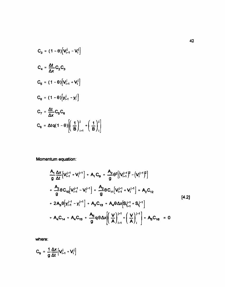
Momentum equation:

4 4 *" + v/" ] + 4 c,* + -0 c,,[v/:; - v/+l] + -8 c,, [v;!, 9 9

where:

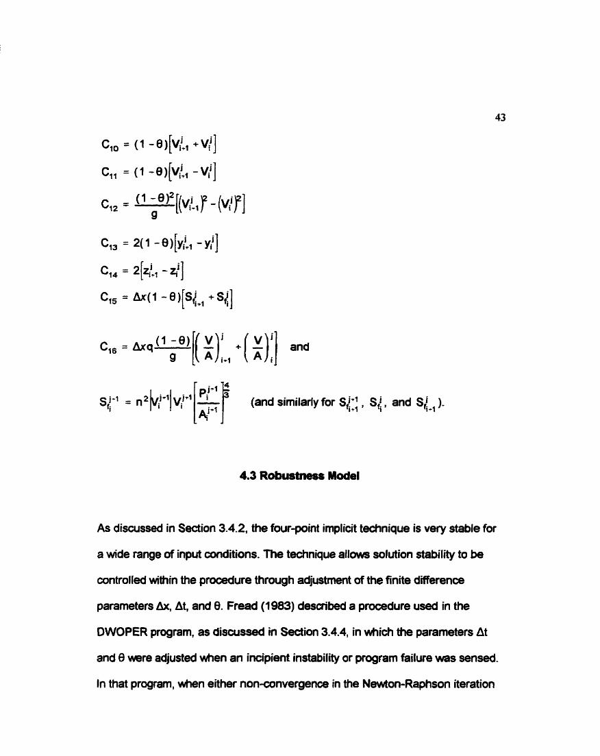
4.3 Robustness Model

As discussed in Section 3.4.2, the four-point implicit technique is very stable for

a wide range of input conditions. The technique allows solution stability to be

controlled within the procedure through adjustment of the finite difference

parameters Ax, At, and 8. Fread (1983) described a procedure used in the

DWOPER program, as discussed in Section 3.4.4, in which the parameters At

and 8 were adjusted when an incipient instability or program failure was sensed.

In that program, when either nonanvergence in the Newton-Raphson iteration

44

or an erroneously low computed depth was detected, an automatic procedure

was initiated to first reduce At, and then to increase 8 in order to increase the

stability of the solution. Although effective in increasing solution stability

generally, the solution technique described by Fread (1983) ~ l a s subject to

failure under certain Row conditions for which adjustment af At and d was

insufficient to prevent program failure.

As discussed in Chapter 2, the objective of this wrk w s to investigate the

potential for a very robust version of the four-point implicit technique in which

severe instabilities developed in the solution were sufficiently suppressed that

program termination was avoided. In addition to adjustment of the finite

difference parameters At and 9, the momentum term coefficients, A, and 4

(discussed in Section 3.3), were automatically reduced in order to suppress the

instability introduced by their respective momentum terms. As the values of the

two selected coefficients (A, and 4) w e reduced to zero, the contribution from

the momentum equation acceleration terms (term1 and term2) was reduced to

negligible and the instabilities introduced by these terms eliminated. When the

coefficients were set between zero and one, the contribution ftom the affected

terms was reduced so that any numerical instability introduced by these terms

was suppressed. With coefficients A, and 4 set to zero, the contribution from

the momentum equation acceleration terms was neglected and the solution

technique was a diffusion wave approximate technique. If coefficients A,, A, and

45

4, were set to zero, the acceleration and pressure terms would be neglected

and the solution wuld become a kinematic wave approximate technique.

The initial intent for this work was to reduce the solution from full dynamic

through difhrsion, by reducing cc)efFicients A, and 4 towards zero, and then to

kinematic by reducing A, towards zero as well. The initial condition used for this

work was a steady-state badwater calculation behind a weir. The kinematic

equation describes uniform flow for which the fridion and gravity slopes are

balanced. With coefficients A,, 4 and A, set to zero, the solution technique

would attempt to solve for a zero residual condition where the residual was the

difference between the friction and channel bed slope terms (given zero

distributed inflow). The calculated residuals would then be the difference

between the steady flow inlial condition and the uniform flow condition, which

would always be non zero. Therefore, reduction of the momentum equation to

the kinematic form wuld be unreasonable with a backwater calculation initial

condition.

For this wwk, coefficient 4 was not adjusted since, as discussed above,

application of a kinematic approximate solution was not reasonable with the

selected initial condition. Adjustment of coefficients A, and 4, and hw

reduction af the momentum equation towards the diffusion wave equation, was

investigated. The parameter Ax was not adjusted since interpolation, with a

46

resulting loss of accuracy, would have been required for x-locations between

previous channel sections.

A simplified flowchart of the procedure, illustrating the logic applied in the

robustness model, is shom in Figure 4.1. The logic follows the four-point implicit

finite difference technique except that prior to a solution advancing to the next

iteration, for any specific iteration within a specific time step, the solution was

checked against a specific criteria and, for a positive outcome, an adjustment

was made to a selected parameter (At, 8, A, andlor 4). An example of the

FORTRAN program code was included in Appendix 6.

As illustrated in Figure 4.1, the unsteady flow calculation loop was started

following initialization and calculation of the initial condition. The initial condition

was a steady flow backwater calculation behind the downstream sharp crested

weir. The constants were then calculated based on the depth and velocity values

obtained for either the initial condition or for the previous time step. The Newton

Raphson iteration loop was started and the values of the residuals, the

difference between the fundion values and the theoretically correct value zero,

were calculated and checked against an acceptable minimum value. If all the

residuals, for that time step and iteration, were less than the minimum value, the

I for umtwdy (low I

t I culculate umstanta for 1

m r e 4.1 Program Flowchart

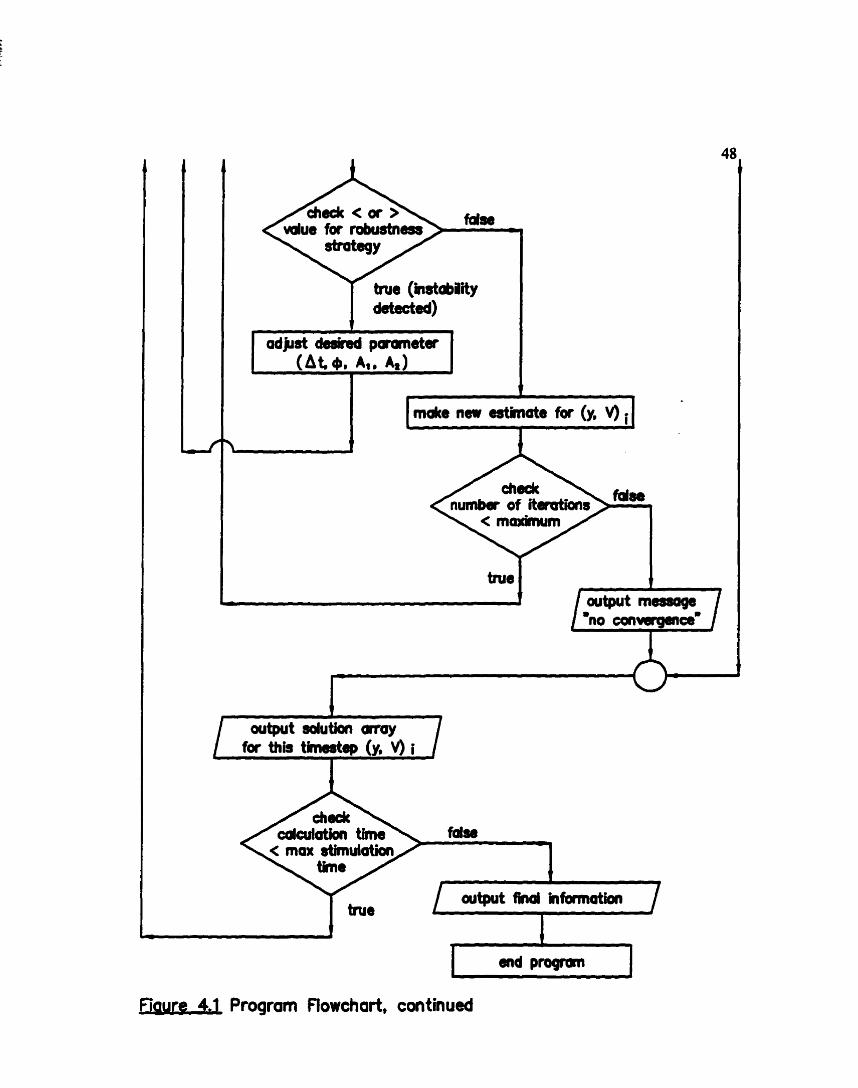
cdculotiorr time < max stimulation

output find informatiron Y / / I

Fiaure 4.1 Program Flowchart, continued

estimate w s accepted as the solution and the unsteady flow loop restarted for

the next time step. For each time step, the solution obtained for the previous

time step was used as the initial estimate for the next

If all the residuals were not less than the minimum value, as ~lould occur at a

time step for which the input flow condition, or downstream boundary, had been

changed, the partial differentials were calculated and a pentadiagonal matrix

procedure used to solve the simultaneous equations. The corrections (Ay and

AV) returned from the matrix solver were then applied to the previous estimate

values to provide the new solution at this time step.

This solution was then tested against the selected robustness criterion. The

criterion was selected to detect a serious instability in the solution prior to

program failure. If the criteria was met, indicating that a serious instability had

occurred, an adjustment was made to the desired parameter (At, 8, A,, or 4).

After the adjustment, the constants were recalculated using the adjusted

parameter(s), the Newton iteration loop was re-entered, and the process was

repeated. Wth this procedure, the programmed model provided a full dynamic

solution at all time steps except those for which a numerical instability was

detected by the selected criterion.

In order to detect a numerical instability, and incipient program failure, a

procedure was programmed to check whether a selected criterion was met for

any time step calculation within the solution procedure, as described above.

When the seleded criteria vws met for the first time within a given time step, At

was reduced by haw and the computation for that time step repeated. As

discussed in Section 3.4.2, such a reduction of At reduced the Courant number,

which shifted the calculation towards the stable condition defined by Cn = 1.

If the instability criteria was met again, 8 was increased to 0.6, with At kept at

one-half, and the computation again repeated. If the criteria was met for a third

time, e was adjusted to 0.8. If the criteria was met again, coefficients A, and A,

were gradually reduced from one towards zero. These coefficients wre kept

equivalent for the initial investigation. Possible adjustments, applied in

subseqwnt calculations when the criteria continued to be met, were to 0.8, 0.5,

0.3, and 0.7. After each adjustment, a solution for the affected time step was

At again attempted, using - and 8 = 0.8. If the criteria was not met, indicating that 2

there were no severe numerical instabilities, the solution w s accepted and the

parameters reset to their original values for the next time step calculation. A

maximum 0 value of 0.8 was selected to minimize dispersion of the solution.

Experiments showed that the applied adjustments were virtually identical

51

whether 0.8 or 1.0 was used as the maximum adjusted value for 8; however, the

dispersion effect of the large 8 value was noticeably less with a 8 value of 0.8.

4-3.3 Selected Criteria

Two criteria wre selected to test for numerical instability and incipient program

failure and thus to determine the time steps for which a parameter adjustment

was made. The selected criteria were: (1) an erroneous solution for which a

channel depth less than zero (y c 0) was calculated, and (2) a supercritical flow

condition for which Froude number was greater than one (Fr > I ). These tww

criteria were used in separate simulations so that a comparison could be made

of the adjustments and affected time steps. These were selected

because they were effective in selecting time steps for which numerical

instability occurred and they were theoretically reasonable. The depth in the

channel should not be less than zero and the channel and boundary conditions

were selected for conditions of subcritical flow.

Several other potential criteria were investigated but with disappointing results.

Both Reynolds number and Courant number were tested, but neither was found

to indicate the time steps exhibiting instability for the tested flow conditions.

Actual values of various momentum equation terms Illrere also tested, however

no consistent numeric value was found which was applicable to a variety of time

52

steps. For the tested flow conditions, the same value d momentum equation

terms was reported for time steps with and without instability. Rather than an

actual value, a relative change in value of one or more of the momentum terms

might prove possible as a criteria. Such an investigation was beyond the scope

of this work since the terms would be expected to vary with different flow

conditions and this wwk was intended to be a general application of improved

robustness rather than specific to the flow and channel conditions tested.

Several different values of Froude number (0.5,2,3) were also tested, and

although parameter adjustments were applied to slightly different time steps in

each case, no clear justification was found for one value over another. The

criterion of Froude number greater than one vms selected since it indicates the

theoretical boundary between submitical and supercritical flow conditions.

4.4 Parameter Selection

The stability and convergence of the model were assessed by varying the finite

difference parameters, & At, and 0, which affect the stability of the solution.

Using the selected channel characteristics, these parameters were varied until

the solution appeared stable and convergent Calculations of Courant number

(See Section 3.4.2) w r e based on the kinematic wave speed. Lateral inflow was

set to zero for all conditions evaluated.

Channel characteristics were selected so that a realistic channel w s

represented in the model. The selected channel was a redangular, prismatic

channel (B = 3 rn) with a fairly smooth (n = .OW) and fairly steep (S, = .001) bed

so that the unstable conditions necessary to test the robustness program vmuld

be relatively easy to create. In order to ensure adequate detail near the

downstream weir, Ax was set to 1 m for 20 rn from the weir and was not varied in

this region.

For investigation of the effect of the finite difference parameters & At, and 0,

the inflow hydrograph was set to a constant 5 m31s and the downstream weir

height changed in height instantaneously from 1.5 rn to 1.0 m tw minutes into

the simulation. Each parameter was then varied while the others were held

constant. First, Ax was varied, while holding At and 0 constant, then At was

varied with Ax and 8 constant, and finally 8 was varied between 0.5 and 1 .O, with

Ax and At held constant The impact of the variation of the momentum

coefficients, A, and 4, affecting the acceleration terms, was then investigated

using the previously determined values of Ax, At, and 8.

54

The results of the investigation into the MBds of varying the parameters Ax, At,

8, and A, and 4, were illustrated in Figures 4.2 to 4.5. The figures were plotted

for a modelled distance approximately haw the distance between the upstream

and downstream boundaries. The results verified previous work and theory since

the most stable and reasonable solution was obtained with At and Ax selected to

provide Cn = 1.0, with 0 greater than but dose to 0.5, and with A, and A, equal

to 1.

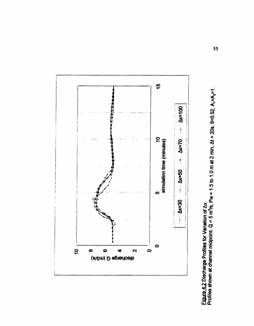
The variation of Ax around 70 rn, to produce Courant numbers very different

from 1.0, caused instability to be introduced into the solution, as illustrated in

Figure 4.2. The solution appeared stable and smooth for Ax = 70 m,

corresponding to Courant number betwen 1.0 and 1.2. When Ax was increased

to 100 rn (C, = 0.1) or reduced to 30 rn (C, = 2.2), the solution showed

instabilities in the form of overshooting at the peak and steps in the previously

smooth curve. For the large Ax, the resulting profile was substantially altered in

shape suggesting that this increment was too large to properly detail the Row.

The instabilities were only apparent for times near the abrupt change in the

inflow hydrograph. For later times, the various Ax profiles were similar showing

the reflection back from the weir at about 12 minutes.

The effect of variation d At, with Ax set at 70 m as determined in the previous

step, was illustrated in Figure 4.3. The result was similar to that for Ax with the

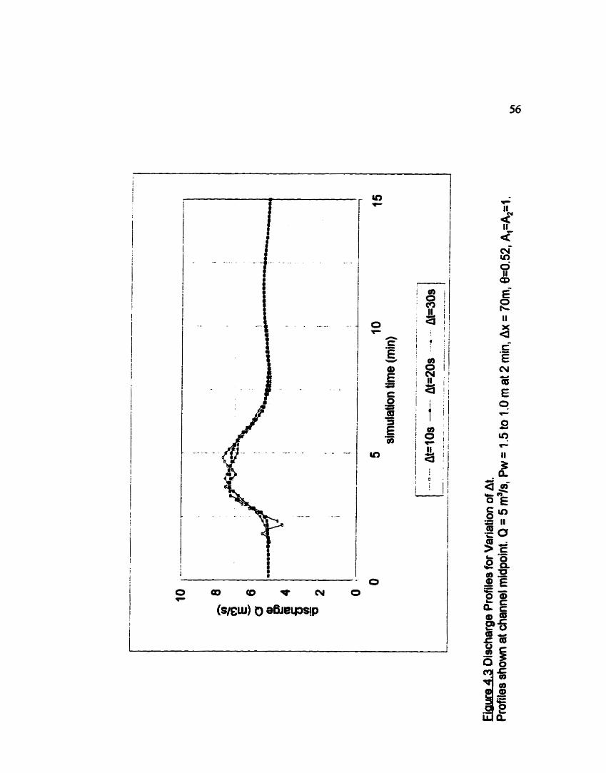
mi- *

57

most stable solution obtained with At = 20 s (C, = 1.0). A reduced At of of 0 s (C,

= 0.5) caused instabilities resulting in a distinctly stepped curve, overshooting

and searching at the peak, and undershooting as the hydrograph started to rise.

A further reduction of At caused very large spikes in the solution and finally

caused the program to fail. Again, the instabilities were observed near the time

of the change in inffow.

The effect of variation of 0, with Ax = 70 m and At = 20 s as previously

determined, was illusttaled in Figure 4.4. Stable solutions were obtained for 8 =

0.55,0.6, and 0.8. With 0 greater than 0.55, dispersion of the wave was

apparent with the peak flattening and widening more severely as 0 was

increased towards 1. With e = 0.5, the solution showed instability producing a

seriously stepped curve. This instability continued for the full duration of the

simulation. As suggested by theory, the best solution, stable and without obvious

dispersion, was obtained &th 8 = 0.55. When 0 was reduced below 0.5, the

program failed.

The effect of varying the momentum coefficients A, and 4, with the other

parameters as previously selected, was illustrated in Figure 4.5. The most

accurate solution w s expected for A, = 4 = 1.0 since the full dynamic

equations were solved in that case. The parameters selected above (&=70m,

At=20s, 8=0.55) provided a smooth curve with A, = 4 = 1, which included the

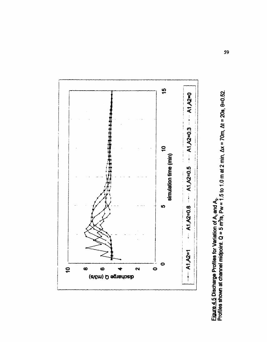
cu- m

60

reflection effect from the downstream weir at about 12 minutes. With A, and 4

reduced belaw 1.0, the entire solution urns shifted to an earlier time and the peak

increased and narrowed. The weir refledion was still evident although increased

in amplitude and also shifted to an earlier time. A similar effect was reported by

Smith (1 980) who found the length of gradually varied flow profile was reduced

with an approximate model. As previously discussed, the solution technique

used for this work was a full-dynamic method when all coefficients (A, to &)

were set equal to 1, and the approximate diffusion technique when A, and A,

were reduced to zero.

When A, and 4 were reduced to zero, the solution became somewhat unstable

and appeared to search betwen extremes causing a stepped discharge profile.

The weir reflection w s no longer reported clearly since a diffusion technique

solution can only approximate effects in the downstream direction. As discussed

in Section 4.3, only coefficients A, and 4 were varied, and these were kept

equivalent for this portion of the work

Results from this investigation suggested that the best solution parameters for

this channel and conditions ware the following: Ax = 70 m, At = 20 0, 8 = 0.55,

and A, = A, = 1. Assuming the celerity of a kinematic wave, these parameters

provided a Courant number very close to one for these flow conditions. In order

to enhance the potential instability, so that recovery couM be tested, the

61

parameters selected for the rest of this wwk were as follows: Ax = 50 m, At = 20

s, and 9 = 0.52, which provided a Courant number of slightly more Wan one

under these flow conditions. Wthin 20 m of the downstream weir, Ax was set at

1 m- The values of Ax Here not varied-

4-4-3 Stable Flow Condition

In order to verify that the model w s successful, and to provide a comparison for

the later unstable solutions, the channel characteristics and finite difference

parameters selected above were used to determine a flow condition which

provided a stable full dynamic solution. The selected flow condition was a

constant inflow hydrograph at 5 m31s with adjusted weir height from 1.5 m to

1 -0 m at 0.5 minutes. The resulting full dynamic solution, plotted at the indicated

locations along the channel, was shown in Figure 4.6. The discharge profile

indicated a fairly stable solution. Some instability was evident on the rising limbs

of the profiles where a sawtooth wave was apparent Of interest to the

discussion of Section 4.4.4 below, the rising limb of the discharge profile

occurred at about 3 minutes for the 750 rn x-location discharge profile.

4.4.4 Contnbutm of Momerlfum Eg~lat . *

ion Terms

The contributions, and relative significance, of momentum equation term1

63

through term4 for the stable flow condition described above was shown in Figure

4.7. The values plotted for each term were from distance location X = 750 rn.

Term5 was zero for this work since it represented lateral inflow, which was set to

zero initially. (l%e momentum equation terms were defined in Section 3.3.)

Term4, the combined fridion and gravity force term, remained fairly constant

throughout the simulation at a value of about -0. I. The sign of the term indicates

that gravity effeds dominate fi-iction effects, since term4 is proportional to

Sf - Sol as expected for subcritical flow conditions. For most of the simulation

time, terrn3, the pressure force term, contributed a value of about 9.1, virtually

balancing the contribution of term4. The positive value of this term, proportional

to byl indicated that the depth ~ l a s increasing downstream, as expected 6x

towards the weir, except for a moment when the pmfile reversed. Term1 and

terrn2, the local and convective acceleration terms, respectively, contributed

virtually zero for most of the simulation, except near the time at which the

change in weir height was applied. A dramatic change in the values of the

acceleration terms, tennl and tenn2, and the pressure term, term3, occurred at

about three minutes into the simulation.

The values of term1 and term3 were Mected dramatically while the value of

term2 w s affected to a lesser degree. The changes in term1 and term2 were

positive while the change in term3 was negative and the values of these

65

changes were such that the sum of the terms remained close to zero. The

changes in tern3 w r e balanced by the sum of the changes in term1 and term2

As mentioned in Section 4.4.3 and as shown in Figure 4.6, the rising limb of the

discharge profile also occurred at a time of about 3 minutes. The simultaneous

occurrence of a dramatic change in discharge profile and in the values of term1

and term2 suggests that numerical instability in the solution can be reduced by

reduction of coefficients A, through 4.

CHAPTER 5. NUMERICAL EXPERIMENTS

5.1 Introduction

Numerical experiments were performed through repeated application of the

model. Several unstable flow conditions were selected for which program failure

could not be prevented by adjustment of the traditional stability parameters of At

and 8. Adjustment of coefficients A, and 4, as well as At and 8, was then

applied for these flow conditions and program failure prevented. The stable full

dynamic solutions discussed in Section 4-4.3 provides a comparison for the

unstable solutions obtained here.

5.2 Results

For unstable condition #1, flow conditions were selected for which a full dynamic

solution could be obtained with adjustment of At and 0. For unstable conditions

#2 and #3, flow conditions were chosen for which a hlll dynamic solution auld

not be obtained. To obtain a solution for these conditions, adjustment of A, and

4 as well as At and 8, was required. The various flow conditions are

summarized in Table 5.1. The automatic procedure programmed into the model

caused application of parameter adjustments according to the two selected

criteria, y < 0 and Fr > 1 (as described in Section 4.3). The parameter

input change wir change channel flow Q at time Pw attime L

condition (m3/s) (min) (m) (min) (m)

Table 5.2 Applied Parameter Adjustments

flow Fiure condition

nitial parameters:

intitial criterion solution timesteps Cn applied resutt affected

failure y e 0 success 59-60 Fr> 1 success 46-91

failure Fr > 1 failure Send y e 0 success 15 Fr> 1 success 3-21

failure y e 0 success 26-43 Fr> 1 success S32

adjusted parameters & theta Al=A2

adjustments applied for solution are summarized in Table 5.2.

5.7.1 Unstable Full Dynamic SQLUtion

Flow conditions for 'unstable condition #I' included a constant inflow hydrograph

at 5 m3/s and a sudden decrease in weir height from 1.0 m to 0.5 rn at 0.5

minutes. Channel length was 1200 m. The partial profile obtained without

adjustment of any parameters, with an insipient instability in the X = 50 m profile

just before program failure, was shown in Figure 51 . The complete profile

obtained with automatic adjustment of At applied according to the criteria y c 0,

was shown in Figure 5.2. The complete profile obtained with automatic

adjustment of At and 9 applied according to the criteria Fr > 1 was included in

Figure 5.3. For this flow condition, adjustment of the traditional parameters of At

and 8 was sufficient to prevent program failure so that a full dynamic solution

was obtained throughout the simulation.

Flow conditions for 'unstable condition #2' included a sudden increase in the

inflow hydrograph from 2 m3/s to 5 m3/s and a sudden increase in weir height

from 0.5 m to 1.0 m, both at 0.5 minutes. Charnel length was 800 m. The partial

profile obtained without adjustment of any parameters, with an insipient

instability in the X = 50 m profile just before program failure, was shown in

Figure 5.4. The partial profile obtained with adjustment of only the traditional

parameters At and 0 HOS shown in Figure 5.5. This result suggests that a full

dynamic solution under these conditions was not possible due to instability

causing program failure. The complete profile obtained with automatic

adjustment of A, and 4, as well as At and 0, applied according to the aiteria

y < 0 was shown in Figure 5.6. Although significant instability is still apparent in

the solution, a solution was obtained without program failure. The instability was

observed to coincide with tirne steps to which no parameter adjustment was

applied. This result suggests that the y c 0 criteria did not identify all the tirne

steps for which numerical instability occurred. The complete profile obtained with

automatic adjustment of A, and A, as well as At and 8 applied according to the

criteria Fr > 1 was shown in Figure 5.7. Substantially less instability was

apparent in this solution suggesting that the adjustments were applied to more

appropriate time steps. Again a solution was obtained without program failure.

The solution appeared smoothed, suggesting that solution accuracy may have

been reduced and that the Fr > 1 may have applied the parameter

adjustment at too many time steps. Wth the criteria Fr > 1, reduction of A, and

4 to a value of 0.5, as indicated in Table 5.2, was sufficient to suppress the

instability and allow program completion. With the criteria y c 0, reduction of A,

and A, to a value of 0.1 was required to sufficiently reduce instability- Since the

criterion Fr > i applied adjustments to a broader range on time steps, the

77

occurring instability may have been reduced allowing a less sever reduction af

A, and 4- Flow conditions for 'unstable condition #3' involved a sudden increase

in inflaw hydrograph from 2 m3/s to 5 5% and a sudden increase in weir height

from 1 .I rn to 1.3 m, both at 0.5 minutes. Channel length w s 1200 m. The

partial profile obtained without adjustment of any parameters, with an insipient

instability in various profiles just before program failure, was shown in Figure

5.8. A complete solution was not obtained with adjustment of At and 8 only. The

complete profile obtained with automatic adjustment of A, and 4 as well as At

and 8 applied according to the criteria y c 0 was shown in Figure 5.9. Some

instability was still apparent in the solution and, again, this instability was

observed to coincide with time steps for which no parameter adjustment was

applied. The complete profile obtained with automatic adjustment of A, and A, as

well as At and 8 applied according to the criteria Fr > 1 was shown in Figure

5.10. Again, little instability was apparent in the solution suggesting that the

adjustments were applied to the appropriate time steps.

3 AQStment of Coefficients 4=A,

An investigation of the relative significance of the hm acceleration terms, term1

and term2, was completed by allowing adjustment of only one of the respective

coefficients, A, and A,, at a time. The same unstable ffow conditions were used

as reported above and summarized in Table 5.1. For unstable flow conditions

81

Zb, Zc, and 3b, adjustment of coefficient A, alone resulted in program failure. For

these same flow conditions, adjustment of coefficient A, alone ~ l a s successful.

For conditions 2b and 3b, with applied criteria y < 0 and Fr > 1, respectively, to

prevent failure, adjustment of 4 alone w s required for more time steps than

required in the solution with both A, and A, adjusted. For condition 2c with

criterion Fr > 1, however, adjustment of 4 alone occurred for f-r time steps

than required in the solution with both A, and A, adjusted. For unstable flow

condition 3a, with criteria y < 0, the opposite was true. Adjustment of 4 alone

resulted in program failure, Mi le adjustment of A, alone provided a solution with

fewer adjusted time steps than the solution with adjustment of A, and A,

together.

The results of this investigation were thus inconclusive since the significance of

the terms was not consistent Results indicated that in order to prevent program

failure, different acceleration terms required suppression for different flow

conditions.

CHAPTER 8. SUMMARY AND CONCLUSION

Using the widely accepted, four-point implicit, finite difference technique to solve

the full dynamic, St Venant equations for gradually-varied, open-channel,

unsteady flow, an extremely robust single-reach simulation model was

developed. This 'robustness model' was used to investigate a potential method

of avoiding program failure by suppressing the severe numerical instabilities

developed in the solution procedure under certain flow conditions. An instability

criterion was used in the model against which the solution obtained within the

numerical technique was automatically checked. This check was performed for

each time step, as the calculations progressed- If the criterion indicated

instability in the solution, an automatic procedure ~ l a s commenced in which

solution parameters were adjusted to suppress the instability. Robustness was

enhanced with this technique so that a solution was successfully obtained under

flow conditions which otherwise caused the program to fail.

The addlional robustness was created within the four-point technique by

assigning a multiplicative coefficient to each of the terms in the momentum

equation and then reducing the value of some of these coefficients t m r d s zero.

The contribution of the term($) affeded by the coefficient(s) was thus reduced for

those time steps for which the selected instability criterion was met Reduction of

coefficients A, and A, which -re applied to the two acceleration terms in the

momentum equation, was investigated fw the tested flow and channel

conditions,

As coefficients A, and 4 wre reduced fmm one towards zero, the solution

proceeded from the full dynamic towards the diffusion technique. Theoretically,

the solution could be taken from the full dynamic through the diffusion to the

kinematic, with adjustment of 4 as well; however, the flow and boundary

conditions used for this work were incompatible vrith the uniform Row modelled

by the kinematic equation. In the diffusion technique, the hrvo acceleration terms

are neglected while with the kinematic technique, the acceleration and pressure

slope terms are neglected. In the robustness model, when A, and 4 are set to

zero, the solution procedure uses the difision equation; and, if A,, 4, and A,

were set to zero, the procedure solves the kinematic equation. In this way, the

model provides a solution of the full dynamic equations for all time steps except

those selected by the criterion as exhibiting instability. For those time steps

meeting the instability criterion, an approximate solution is provided. By applying

the parameter adjustments for only those time steps for which the instability

criterion is met, a full dynamic solution is obtained for all possible time steps so

that the best possible accuracy is maintained throughout the simulation.

As discussed by Fread (1983), the stability of the fourgoint technique can be

enhanced within a simulation by reducing the value of At, thus reducing the

Courant number, or by increasing the value of 0. The criterion used by Fread

was y c 0, and the adjustment was applied automatically when the criterion was

met. With adjustment of At and €I8. a full dynamic solution was provided. Fread

reported flow conditions for which these adjustments were insufficient, but he did

not report investigation of a method to further increase the stability of the

solution. In the work for this thesis, adjustments were applied to At and 8 initially

and then, for time step solutions which continued to meet the instability criterion,

the values of the coefficients A, and 4 were gradually reduced. The cxlefficients

were reduced in value between one and zero depending on the persistence of

the instability. The tested unstable flow and channel conditions caused the

program to fail when only At and 0 were adjusted, but allowed a successful

solution when A, and A, were also adjusted.

Adjustment of the coefficients was done automatically within the program when

the solution obtained for a given time step met the selected instability criterion-

Two different criteria were successfully tested to suppress instability Mi&

othewise caused program failure, and several others mre investigated. The

successfully used criteria were (1) depth less than zero (y < O), and (2) Froude

number greater than one (Fr > I). Both were used effectively in

preventing program failure which otheMse occurred for the same flow

conditions with adjustment of At and 9 only.

85

The criterion Fr > 1, appeared to cause reduction of the momentum equation

coefficients, A, and 4, to occur more frequently than may have been necessary-

Several other values of Froude number w r e tested, however none was found

satisfactory. The criterion y c 0, appeared to miss some time steps for which

significant instability, although not sufficient to cause program termination,

developed in the momentum equation acceleration terms. This result was

expected since only negative instability 'spikes' reaching zero depth would be

detected leaving positive instabilities unaffected.

In order to improve the stability of the solution technique, some of the accuracy

of the full dynamic solution was traded for increased robustness. The method of

adjusting the coefficients developed for the robustness model, and the reduction

of the solution from the full dynamic towards the diffusion technique, provided

the desired additional robustness. The success of the tested procedure in

preventing program termination indicates that development of a widely

applicable and extremely robust version of the four point implicit finite difference

technique is practical. Such a model would allow application of the best

available technology, a full dynamic technique, so that an accurate solution

could be obtained even under difficult flow conditions. Current standard

engineering practice indudes application of an approximate model, often a

steady-state or kinematic model, for the full duration of a simulation when Row

conditions cause solution instability. Through the work for this thesis, a method

86

to switch from a solution of the full dynamic equations to an approximate method

and back again within a simulation run, and to apply the approximate technique

for only those time steps exhibiting numerical instability likely to cause program

failure, has been identified. This technique could change the entire approach to

open channel flow modelling by eliminating the use of approximate method

simulations in welldefined channels.

Only full dynamic simulation methods provide sufficiently accurate solutions to

problems of open channel design and operation to address the issue of

efficiency of use. In a world where water and financial resources are becoming

more scarce and more valuable, the efficiency of water conveyance structures is

of increasing importance. The potential benefit of widespread use of the

accurate solutions provided by application of full dynamic simulation methods is

efficient design and operation of conveyance systems and accurate prediction of

flood events.

CHAPTER 7. DISCUSSION AND RECOlUMENOAl'lONS

For open channel flow modelling, the use of approximate techniques, which

provide a solution to an approximation of the full dynamic equations of open

channel flow, is accepted as standard engineering practice. Commonly used

approximate models include the diffusion, kinematic, and steady flow

techniques. As discussed throughout this thesis, the diftrsion and kinematic

techniques approximate the momentum equation by neglecting the acceleration

terms and the acceleration and pressure slope terms, respectively. Removal of

these terms is based on the assumption that their contribution to the solution is

negligible. The results of the investigation undertaken for this thesis suggest that

the contribution from these terms is significant for the Row and channel

conditions modelled in this wrk As well, the results suggest that neither the

diffusion nor the kinematic technique is reasonable for many applications of

open channel flow in WII defined channels.

Without the acceleration terms w the pressure slope term, the momentum

equation, as used in a kinematic solution procedure, is simply the equation for

uniform flow (for zero lateral inflow), as indicated in equation [3.23]. Uniform flow

wuld only o c a ~ in a very long consistent channel where gravity and fridion

forces were balanced. In an operated canal, channel sections are often fairly

short and are separated by some type of structure or change in channel cross-

88

section. Flow conditions in such an operated channel would likely be affeded by

badwater effects, such as reflections from a channel constriction, so that

uniform flow wu ld not occur. A kinematic technique, therefore, wuld not be

appropriate for such channel and flow characteristics.

The difiusion equation neglects the acceleration terms but includes the pressure

slope term so that backwater Meds can be approximated. However, results from

the robustness madel developed for this thesis indicated that with the hho

acceleration term coefficients, A, and 4, set to zero, numerical instability ~ l a s

introduced into the solution. This result demonstrated that a term other than the

acceleration terms was responsible for this instability. The investigation of the

acceleration and pressure slope terms indicated that all three terms ware

affected by instability when a rapid change in input flow conditions occurred in

the model, as discussed in Section 4.4.4. By neglecting the acceleration tems

(terml and tern), and the pressure term (term3), the momentum equation was

left unbalanced so that the contribution of one term wes not reduced by an

opposite contribution from another. In the derivation of the momentum equation,

the sum of the terms (terml through terrn5) was set to zero. Clearly, when some

terms are neglected, this assumption can only be true if the values of the

neglected terms are near zero. Where rapid changes in input flow conditions

occurred, the results of this work indicate that the values of the acceleration

terms are not sufficiently near zero to justify neglecting the tems completely. In

89

addition, the results indicate that the sun of the acceleration and pressure slope

terms is necessary to produce a correct solution. These results support the

recommendation af Weinmann (1 977) that the acceleration terms are important

for steeply rising or falling hydrographs. Use of a diffusion equation technique,

therefore, must be questioned for simulation of changing flow conditions. The

robustness model allowed the use of an accurate, full dynamic solution with

application of the less-accurate diRusion technique only at those time steps for

which the calculation exhibited numerical instability.

Approximate methods may be useful for flow conditions with little variation in

channels of Rat bad slope and relatively unknown cross-section. In umll4efined

channels with varied flow conditions and numerous structures, only a full

dynamic solution can provide a correct result. Irrigation systems generally have

very regular and known cross-sections and controlled, variable flow conditions.

In order for such a system to be efficiently designed and operated, so that

construction, operation, and maintenance costs are minimized while available

water supply is maximized, an accurate hrll dynamic simulation model is

required. The success of the robustness model developed for this thesis work

indicates that an extremely robust model can be developed to provide a solution

for the full dynamic equations throughout the simulation except for those time

steps which exhibit numerical instability sufficient to otherwise cause program

failure. For those time steps, the method provides a solution for an approximate

momentum equation.

Several potential criteria for identifying the time steps aff8ded by severe

numerical instability were investigated. Although the Wm criteria used for this

work were successful in preventing program failure, additional criteria could be

investigated in order to determine the one(s) that provides the most effective

selection of time steps for which to apply the approximation. Application of the

coefficient adjustment to too many time steps results in a less accurate solution,

while application to too few time steps results in severe instability affecting the

solution or causing program failure. In order to develop the best possible criteria,

the contribution of the various momentum equation terms, for a variety of flow

and channel conditions, needs to be fully understood so that their appropriate

contribution can clearly be distinguished from instability.

Through the investigations completed for this thesis work, the following areas

were identified for further study:

1. Investigation of other potentially usefbl criteria for automatic application of

coefficient adjustment and determination of the most effective criterion under

various flow conditions. Possible criteria could include the magnitude or change

in magnitude of the various momentum equation terns.

91

2. lnvestigation of the significance of the various momentum equation terms on

numerical instability and of the relative magnitude and sign of terms under

various flow and channel conditions.

3. Investigation of the eRed on solution accuracy of using an approximate

technique briefly within the full-dynamic solution. The approximate technique is

known to move events earlier in time and to reduce the effects of attenuation

and wave reflection, and a quantitative study of these effects on the overall

solution wuld be of value-

4. Investigation of reduction of the other coeffidents, &, &, and &, as

applicable for various flow and boundary conditions.

92

LITERATURE CITED

Arnein, M. (1 968). An implicit method for numerical flood routing. Water

Resources Research, & 71 9-726.

Canadian Society for Civil Engineering Task Committee on River Models.

(1 990). Comparative evaluation of river models. Proceedinas of the Annual #

Conference of the CSCE. Hamilton, Ontario. V, 282-300.

Chow, V. T. (1 959). Open-Channel Hvdraulics. New York: McGraw-Hill Book

Company.

Chow, V. T., Maidment, 0. R., & Mays, L. W. (1988). &plied Hydrology. New

York: McgmwHill Book Company.

El-Maawy, AA 1991. Weiahted Four - Point Imo licit Method of Solution the St.

Venant Fauations, University of Calgary, Calgary, Alberta.

Fread. D. L. (1 973, April). Effects of Time Step Size in Implicit Dynamic Routing.

American Wate . . r Resources Assoc~at~on. Water Resources Journal, s(2). 338-

351.

93

Fread, D L (1 981 ). Numerical Hydrodynamic Modelling of Rivers for Flood

Forecasting by the National Weather Service. proceediqp of the International

nfer ce of m ~ C h a n c a l n e l . andove r 1 and F low for

Water Resources and Fnvironmental qR~licationq- Bratislava, Czechoslovakia.

French, R H. (1 985). Open-Channel Hv-uIicg. New Yo* McGraw Hill Book

Company.

Henderson F. M. (1966). Open Channel Flow. New York- Maanillan Publishing

Company.

Huber W. C. 8 Dickinson RE. (1 988). S s

Model. Version 4. US. Environmental Protection Laboratory. Athens, Georgia.

Lai, C. (1986). Numerical Modelling of Unsteady Open-Channel Flow. Advances

in Hvdroscience, 14,161-344.

Maw, D. H. (1 994). Modelling Irrigation Conveyance Systems using the JCSS

Model. prwdi-wert C o n s w n an I m p

Models. Rome, Italy.

Manz, D. H. (1 991). [Open Channel Hydraulics]. Unpublished course notes for

End 725, University of Calgary, Calgary, Alberta.

Robertson, J. A 8 Crowe, C. T. (1985).+Dgineerina Flyid Wanics. Boston:

Houghton Mifflin Company.

Rowney, AC. 8 Maaae, C.R. (1 991 ). Qualhymo Users Manual. Release 2 . 1 -

The Royal Military College of Canada, Dept of Civil Engineering, Kingston, Ont.

Smith, A. A (1 980). A Generalized Approach to Kinematic Flood Routing.

Journal of &&&gy, Amsterdam: Elsevier Scientific Publishing Company.

Weinrnann, P. E. (1977). Comparison of Flood Routina Methods for Natural

Rivers. Monash University.

Wisner, P. (1 989). Intern o/OUhymo 89. University of Ottawa, Department of

Civil Engineering. Ottawa.

US Army Corps of Engineers Hydrologic Engineering Center. (1995.) HEC - RAS

River Analysis Svstem H v w i c Reference Manwl - DrM. Davis, CA: Author.

95

APPENDIX A FOUR-POINT IMPUCIT FINITE DIFFERENCE TECHNIQUE

The St Venant equations used for this work, derived in Section 3.2, descri-be

one-dimensional, unsteady, gradually varying, open charmel flow and are

applicable for cases which comply with the assumptions specified in the

derivation. The two full dynamic equations, [3.3] and [3.23], were discretized for

numerical solution as described below. The four-point implicit finite difference

scheme was used to replace the non-linear partial differential St Venant

equations with a set of 2N non-linear simultaneous equations. The generalized

Newton iterative method was then used to reduce the set of non-linear equations

to a set of linear equations for solution.

A1 Distance lime Grid

At a point m on the distance-time grid show in Figure Al, and located entirely

within the comer grid points (i, j), (i+1, j), (i, j+1), and (i+i, j+l )as shown, any

variable a is defined as (Mant, 1991 ):

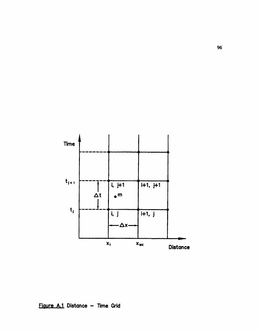
Distance

mure A.1 Distance - Time Grid

where, 8 is the weighting factor.

The subscripts I and j represent the position along the distance axis and the time

value, respectively, so that the velocity at any point and time is represented by

v,', for example. At time j, all values are known from the previous time step

calwlation, so that the unknowns, velocity and depth, occur at time j+1. The

governing continuity and momentum equations (Equations [3.3] and [3.23]) must

be satisfied at the point m. The finite difference operators, specified by

equations [All, [A.2], and [A3], were applied to these equations with the results

indicated below.

A2 Continuity Equation

The non-linear partial differential continuity equation used for this wwk was:

Application of the above finite difference scheme to equation [3.3], with

simplification, provided the following disaetized version of the continuity

equation:

where:

A3 Momentum Equation

The non-linear partial differential momentum equation used for this work was:

This equation included the multiplicative coefFicients applied for each of the

momentum equation terms and used to investigate the robustness of the solution

technique, as discussed in Section 3.3. Application of the above finite difference

scheme (Equations [A I], [A2], and (A.31) to equation [3.23], with simplification,

provided the following discretized version of the momentum equation:

where:

s j - 1 = n2 i-1 ,itl fi /vl 1 , [PI' (and simiuny n q+l s i . m a sj 1. and. 4"' +1 1-1

So = (' - '" ) , where z is the elevation hPrn e reference datum, Ax

and where the following are constants wing known (time j) values of the

varia bies:

C,, = (1 -e)[v/+, +v/]

C,, = (1 -O)[V!*, -v/]

114 Solution Procedure

There are (N-I ) points in space like m, shown in Figure A1 , in the distance-time

grid betwen time j and time j+l. The two finite difference equations (Equations

[A41 and [A5]) were written at each point, and the resulting (N-1) continuity

equations and (N-I ) momentum equations were represented by

F, (y,"f , v/" , yK , v / ! ) , and ~~(y! ' ' , v/*', yiy , ~i!;' ) , respectively. The hnro

additional equations required to make the set of 2N equations for the 2N

unknowns (y, and Vi) w e obtained from an upstream and a downstream

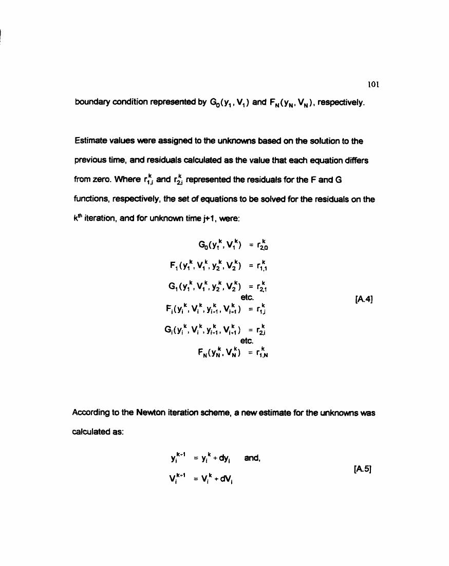
101

boundary condition represented by %(y, , V1 ) and FN ( y, , V, ) , respectively.

Estimate values were assigned to the unknowns based on the solution to the

previous time, and residuals calculated as the value that each equation differs

from zem. Where r:, and r& represented the residuals for the F and G

functions, respectively, the set of equations to be solved for the residuals on the

km iteration, and for unknown time j+i, were:

According to the Newton iteration scheme, a new estimate for the unknowns was

calculated as:

k ' = yi + dyi and,

v y = vik + mi

102

For each time step, the residuals were calculated and checked against the limit

If all the residuals are less than the limit, the solution ( y,, Vi) was accepted. If

any of the residuals was larger than the limit, the partial derivatives of the Fi and

G, equations were calculated and defined as a matrix [A]. The residuals

calculated w r e defined as matrix [B]. A sparse pentadiagonal matrix solution

technique was used to solve the matrix equation [AID<] = [B] for the solution

matrix D(1 which then represented the values of dyi and dVi to be used for the

next estimate of yi and V,. The matrix equation was defined as:

The new estimates were then calculated according to equation [A7], and the

iterative process is repeated until the values of the residuals was less than the

set limit, or a maximum number of iterations was exceeded.

APPENDR B. PROGRAM CODE

The following FORTRAN code w s used for the robustness model:

* Robustness model for thesis - June 1996 - C. Vrkljan * DOUBLE DOUBLE DOUBLE DOUBLE DOUBLE DOUBLE DOUBLE DOUBLE DOUBLE DOUBLE DOUBLE DOUBLE DOUBLE DOUBLE DOUBLE DOUBLE DOUBLE DOUBLE DOUBLE DOUBLE INTEGER OPEN (3

PRECISION QP, QI, SO, m, DELT, SIMTIM, RGO, REM PRECISION TIPE, LTOT, D E W , D E W , SUM, SIML, TXMCRK PRECISION TIM(111, QIN(10), PUPS (100). DELX (100) PRECISION 2 (1001, XST (loo), YANS (100, loo), VANS (100,100) PRECISION YNERT(lOO), YOLD ( l o o ) , VNEW(100) p VOLD(100) PRECISION DELXUN (100) , V 1100 1 , QQ (100) , XANS (100 ) PRECISION G,Q, PIO,B, YW,QIQ,DQW, CE, CW, MAT- (100 PRECISION AA1, PI, SF, E'YI, FPl,XLAST,UDELX, E'R, RE PRECISION AA, PP,YYr QNEIQ(10) , ~RXA(100, loo), QANS (100) PRECISION Y (100) ,E'Y (501, FP(501 ,A(100), P(100). DELTJ(100) PRECISION AOLD (100). POLD (100) ,SFOLD (LOO) , ~ ( 1 0 0 ) PRECISION PNEW(100). SE'NEW(100) ,VAI;UE,!CEA,Al,A2,A3,A4,~ PRECISION Cl(100). C2 (100). C3 (100) ,C4 (100) ,CS (100) PRECISION C6(100),C7(100),C8 (lOO),C9(1OO),ClO(lOO) PRECISION C11(100) ,C12 (100) ,Cl3 (100) ,Cl4 (100) ,CIS (100) PRECISION C16(100) ,RF(100) ,RG(100) ,FMPE'(200) ,MATRXX(100) PRECISION DIEY(100) ,DIEV(100) ,DIGY (LOO) ,DICiV(100) PRECISION FMTA(200 1, E'MTE (200) , FMTD (200) . E'MTC (200) PRECISION FWIN(10) ,TIMP(lO) ,PWJ(100) PRECISION TERMl, TERM3, INTIIA, INAl, INR2, INP3 NQr~,~,MpE,EOLD,UNUS,J,K,N,K~ll,COUNTrCRZT 1, PILE= ' INPUT2. DAT ' 1

OPEN (35, PILE= ' FLOPQIN2. DAT ' ) OPEN (21, FILE='UNST.OUT' 1 OPEN (27, FILE='TEMPLOT-TXT') OPEN ( 28, FILE= ' TERMS, TXT ' )

*

READ (31, * ) QI.QP,B,SO,MANN,LTOT READ ( 3 *) DELXWpDELX2,INTHA, I=, INA2,INA3,DELT,A4,W DELTJ (1) = DELT

* i n i t i a l i z e *

* upstream flow-time and variable weir height READ (35,*) NQ, SIMTIM DO 100 I = I, NQ

READ (35,') QIN(IJ, TIM(1) 100 CONTINUE

READ (as,*) NP DO 101 I - 1, Np

READ (35,*) PPQIN(I) , TIPP(I) 101 CONTINUE

rt number o f time calcs *** M = (SIMTIM * 6 0 . 0 ) / DELT + 1 f Q - time series *** DO 110 J = 1, MJ

TIME = DELT * (J - 1 . ) DO 112 I = 1, NQ

IF ( I .EQ- NQ THEN

END1 F TfMC?XK = TIM(It1) * 6 0 - 0 If ( TIME .LT. TIMCBK ) TE$EN

QUPS(J1 = QIN(1) GO TO 115

END1 F 112 CONTINUE 115 W S = 1

DO 113 1: = I, NP IF ( I .EQ- NP ) THEN

PWJ(J) = PWINCNP) GO TO 116

ENDIF TIMCHK = TIMP(I+l) * 6 0 - 0 IF ( T m .LT- TIMCHK ) THEN

PWJ(J) = PWIN(11 GO TO 116

ENDIF 113 CONTINUE 116 UNUS = 1 110 CONTmuE i

* i n i t i a l i z e for steady f l o w calcs ******************** * EJW = PWIN(1) SUM = 0-OD0 M = (LTOT - 20.) / DEU(2 t 21 WRITE (21,* 'M = ' , M DO 1 2 0 I = 1, M-1

IF ( I .LT- 21 1 THEN DELX(1) = D E W

ELSE DELX(I1 = DELIS2

ZNDX F SIML = SUM + DEIX(1) SUM = SIML

1 2 0 CONTINUE

e verify input IF ( SO -GT- 0.1 THEN

PRINT *, 'WXRNING Channel slope is lacge. S o = ' ,SO WRITE (21, * 1 WARNING Channel slope is large. '

ENDIF IF ( MANN .GT. I THEN

PRINT *, WARNING Mannings roughness i s large. n = *, MNW ENDIF

* boundary condition : sharp-crested weir * negligible viscous and surface tension effects

PRINT *, 'depth at w e i r YW = ', YW PRINT *, 'depth PW = ', PW

* ~r calculate Froude number

FR = ( Q**2 / (G * 8**2 * YW**3) )**0.5 IF ( FR -GT. 1-0 ) THEN

PRINT *, 'Steady f l o w is supercriticalt WRITE (21, * 1 ' Steady flow is supercritical * GO TO 9999

E N D 1 F IF ( FR -EQ. 1-0 ) THEN PRINT *, ' F l o w is criticalr WRITE (21, * I ' Flow is critical '

ENDIF IF ( FR .LT- 1-0 ) THEN

PRINT * PRINT *, 'Fr =*, PR PRINT *, 'Flow is subcritical at weirt PRINT * WRITE (21, *) ' F l o w is Subcritical at weirr

ENDIF *

Z(1) = O.ODO Y ( 1 ) = YW XST(1) = O.ODO Q Q W = Q YY = YW XLAST = 0-OD0 DO 140 I = 2, M

UDEWr = DELX(1-1) XST ( I ) = XLAST + UDELX QQ(1) = Q + (QP-QI) * XST(1) Z ( 1 ) = Z(I) + SO XST(1) A(1-1) = B * Y(1-I) P(1-11 = B + 2-ODOfY(I-1) AA A(1-1) PP = P(1-1) XtAST = XST(I)

$ + (MANN**2) *UDELX* (QQ (I) * * 2 ) $ * (4.ODO * (PP**(l.OD0/3,0DO)) $ / (3,ODO* (AA**(IO,OD0/3.ODO))) $ -5,ODO * (PP**(4.OD0/3.ODO)) * B $ / (3.ODO" (AA**(13-0D0/3.0DO))) ) Y(1) = Y(I-1) - FYI / ET1

*

FP (J) = (-1 - ODO) + B/ (2,0DO*G) $ * ( QQ(1-I)**2/A(I-T)**3 $ + 3.ODO*QQ(I) **2*A(I-1) / A(1) **4 $ - Z-ODO*QQ(T) **2 / A(1) **3 ) $ - (QP-Qf *UDELX*B/G * QQ (I ) /A(I ) **3 $ + MANN**Z*U'DELX*QQ (I) **2 $ * ( (4-ODO*P(I)/ (3.ODO*A(I )**lo) ) $ ** (1-0D0/3.ODO) - (S,ODO*P(I) **4 * B $ / (S.ODO*A(I) **l3) ) **(l.OD0/3,ODO) ) *

YY = Y ( 1 ) - FY(J) / FP(J) IF ( ABS ( YY - Y(1) ) .LT- 0.0005 1 GO TO 160 IF (YY -LT* OeODO) THEN PRINT *, 'Y less than zero i n steady calc at I = ', J WRITE (21,*) *Y less than zero in steady calc at 1 = *, J ENDIF FR = ( Q**2 / (G * B**2 * YY**3) )**0.5

IF (FR .GT. I.ODO) TIEN WRITE (21, *) 'Steady f l o w is supercritical at I = ', J PRINT *, 'Steady f l o w is supercritical at I = ',J GO TO 9999

ENDIF Y ( I ) = YY

150 CONTINUE: PRINT *, 'Steady f l o w calculations did not converge!'

GO TO 9999 160 UNUS = 1 140 CONTIMJE *

PRINT *, 'Steady F l o w calulations completed' PRINT *, ' '

* turn solu t ion around EOLD = 0 DO 200 I = M, I, -I

E = EOLD + I * XANS(E) =XST(I)

YANS ( E , I ) = Y(I) YNEW(E) =Y(I) YOLD(E1 = YNEW(E) VANS (E, 1) = V(1) VNEW(E) = V ( I ) VOLD(E) =VNEW(E)

* IF ( I -GT- 1 ) THEN t DELXUN(E1 = DELX(1-I) * ENDIF

EOLD = E 200 CONTINUE f set unsteady delta-x and distance DO 201 E = 1, M-21 DELXUN(E1 = DELX2

201 CONTINUE DO 202 E = M-20, M-1

D E W C E ) = DELXW 202 CONTINUE XANS(I) = 0-OD0 XANS ( 2 1 = DELX2 DO 203 E = 2, M XANS(E) = XANS(E-I) + DELXUN(E-1)

203 CONTINUE * * s e t elevation 2 Z(1) = S f M L * SO Z (M) = 0-OD0 DO 210 I = 2, M-l

Z(1) = Z(1-1) - SO DEUCUN(1-1) 210 CONTINUE 9r

VALUE = -001 WRITE ( 2 8 , * ) ' J K I tenal tena2 term3 tenn4'

* WRITE ( 2 8 , * ) ' J K I YANS(1) QANSII) TERMl FR RE' WRITE ( 2 8 , * ) ' WRITE ( 2 7 , * ) ' XANS(1)

$ THETA Al' WRITE ( 2 7 , * ) ' '

* e unsteady flow i teration ******************** * DO 500 J = 2 , MJ WRITE (21, * I ' s tart of j-loop J= ' , J

* DELTJ (J) = DELT DELTJ(3-1) = DELT THA = INTHA COUNT = 0 Al -- INAl A2 = 1-

PRINT *, 'J = ' r ‘7 QNEW(1) = QUPS(J) DO 310 I = I, M

AOLD(1) = B * YOLD(1) POLD(1) = B + 2.ODO * YOLD(1) SFOLD(1) = (VOLD(I)**2) * MANN**2

$ ( (POLD(1) /AOLD(I) ) ** (4.0D0/3,ODO) ) SFOLD(1) = ABS(VOLD(1)) * (VOLD(1)) * MANNe*2-OD0

$ * ( (POLD(I)/AOTS(I))**(4,OD0/3.ODO) ) 310 CONTINLJE

CRIT = 0 3 1s m s = 1 * * constants

DO 320 H = I, M-1 CI (HI = (-1- OD0 1 * (YOLD (H+l) + YOLD (H) ) C2 (HI = (1.ODO-TBA) /B * (AOLD (H+1) + AOLD (HI ) C3 (HI = (1. ODO-THAI WOLD (H+I) - V O W (HI ) C4(R) = DELTJ(J-I) /DELXUN(H) * C2 (HI * C3 (H) CS (R) = (1. ODO-THA) * (VOLD (H+I) + VOLD (HI ) C6 (HI = (1 .ODO-THAI * (YOLD (H+I) - YOLD (HI ) C7 (HI = DELTJ(J-l)/DEWZUN(H) * CS(H) * C6(H) C8 (HI = DELTJ(J-1) * (QP-QI) * (1,ODO-THA) *. 2- ODO/B c9 (HI = (-LODO/G) *DELXUN(H) /DELTJ(J-I)

* (VOLD(H+l)+VOLD(K) ) CIO (H) = (1 . ODO-THA) * (VOID (H+1) + VOID (H) ) ClI (H) = (1 . ODO-THA) * (VOLD (H+l) - VOLD (H) ) C12 (H) = ( (1.ODO-THAI **2) / G* ( (VOLD(H+l) **2)

- (VOLD(H)**2) 1 Cl3 (H) = 2.0DOe (1.ODO-THA) * (YOLD(Ei+l) - YOLD (H) ) CT4(H) = 2-ODO*(ZtH+l) - Z ( H ) ) C15 (8) = DELXUN(H)* (1.ODO-THAI (SE'OLD (H+l) +SFOLD (H) 1 C16 (H) = DELXUN(H) / G * (QP-QI) * (l.ODO-TB-1

* Newton Iterative Method ****************** *

* calculate residuals DO 340 H = 1, M-1

RG (H) = A ~ / G *DEWLUN (H) /DELTJ (J) * (VNEOQ (He) +VNEW (H) ) S + X * C ~ (HI + A ~ / G * (THA**2) * ( (VNEW (H+l) **2) $ - m J E W ( H ) * * 2 ) ) $ + AZ/G*THA*Cll (HI * (VNEW(H+l) + VNEW(H) )

RG(H) = RG(H) $ + A ~ / G * T ~ * c ~ O (HI * (VNEPQ (El+-I) - VNEW(H) )

+ A2*C12 (R) + Z.ODO*A3=THA* (YNEW(H+I) - m ( E ) + A3*C13(H) + A4*TBA*DELXUN(H) *(SFNEII(Htl) + SE'NEW(H) + A4*C14 (8) + AOeC15 (HI

+ -/G* (QP-QI) *TBA*DELXUN(B) * ( (+(H+I) / -(B+l) ) + (VNEsr(H) /ANEPT(Ii) ) + A5*Cl6 (g)

=(2*H+l) (-I.ODO)*RG(H)

CONTINUE

set boundary values HkT = YNEW (MI - PWJ (J) CE = -6020DO + -0750DO * HW/PWJ(J) C ' = 2 - ODO/3.ODO *CE * ( ( 2 . ODWG) **0. SODO) IF ( YNEW(M) -LT. PWJ(J) ) THEN QW = O.ODO GO TO 341

ENDIF QW = cw *B * (m**i.50~0)

UNUS = 1 RGO = QUPS(J) - VNEW(I)*ANEW(I) REM = VNEW(M)*ANEW(M) - QW MATRXB(1) = (-1-ODO)*RGO MATRXB (2*M) = (-1 - OD0 ) *RFM

check residuals 350 I = I, 2*M

calculate partials

WRITE (21,*) 'start partials K= ', K DO 360 H = 1, 2*M

DO 361 I = 1, 2*M MA!rRXA(H,I) = 0-OD0

361 CONTI'NUE 3 60 CONTINUE

DO 370 El = 1, M-1 DLGY (HI = (-2. ODO) *A3*THA

$ + 4.OD0/3- 0DO*A4*THAIrDELXUN (H) $ *SEN5W(Hl * (2.0DO/PNEW(H) -B/ANEW(H) ) $ - a* (QP-QI *T~*DELXUN (R) *B/G $ * ( VNEW(H)/(AEElf(H)**2) 1

MATRXA(2*H+lr 2*H-1) = DZGY (H) DIGY(H+l) = 2.ODO*A3*THA + 4.OD0/3.ODO*A4*THA*DELXUN(H)

*SPNEW(fE+I) * (2-000/PNEW(~+l) -B/ANEW(K+l) 1 - As* (QP-QI *TBA*DELXUN (H) *B/G

* ( VNEW(H+I) / (ANEW(H+l) **2) I MATRXA (2*H+1,2*R+l) = DIGY (H+I) DIGV (HI AI/G*DEIXUN (B) /DELTJ (3)

- 2.0DO*A2* (THA**2) / G * VNEW(H) - A2/G*TRA*ClO (HI + A2/GeTHA*CII (Ei) + 2.0DO*A4*THA*DEfXUN (HI *SFNEW (H) /VNEPQ (H) + M/G* (QP-QI) *THA*DElXUN (H) /ANEW(B)

MATRXAtZ*B+l, 2*H) = DIGV (H) DIGV (H+I 1 = Al/G*DELXUN (H) /DELTJ (J)

+ ~.ODO*AZ/G* (THA*'*Z) " VNEW(fl+l) + A~/G*THA~c~O (HI + A2/G*THA'tCIl (H)

DIGV(K+I) = DIGV(H+I) + 2,0DO*A4*TBA+DELXUN(H) *Sl?NEW(fl+l) /VNEW(H+l) + AS/G* (QP-QT) *TBA*DELXUN(H) /ANEOT(H+l)

MATRXA(Z*EI+l, ZtH+2) DIGV (H+l)

D I F Y (HI = 1.-2. *DELTJ(J) /DEDWN(H) * (TBA**2) *VNEW(H) $ + DELTJ (J) / D E I X J N (HI *THA*C3 (8) $ - DELTJ (J) /DELXUN(Ei) *THA*Cs (K)

MATRXA(Z*H, 2*H-1) = DIEY (H) D I F Y (H+1) = 1 - ODO+Z,ODO*DELTJ (J) /DELXUN (H)

$ * (THAe*2) *VNEOQ(Ii+l) $ + DELTJ (J) / D E W ( H ) *TEA*C3 (H) $ + DELTJ (J) /DELXUN (HI *TAtC5 ()I)

MATRXA(2*H, 2*H+1) = DIEY (H+l) DIEV (a) = (-1-ODO) *DELTJ(J) /DELXUN(H) * (THA**2) /B

$ * ( ANEW(H+I)+ANEW(H) ) $ - DELTJ (J) /DEWNN (H) *TE?A*C2 (H)

D I F V ( R ) = DIE'V(H) $ + DELTJ(J) /DELXUN(H) * (THA**2) ( YNEW (X+1) $ -YNEW (HI + DELTJ (J) /DELXUN (B) *THA*C6 (H)

MATRXA(2*Hf 2*H) = DIFV(H) DIFV(H+l) = DEZ;TJ(J) / D E U N N (H) * (TfIA**2) /B* (ANEW(H+l)

$ +-(HI 1 S + DELTJ (J) /DEIXJN (H) *TH?%*C2 (H)

D I F V ( H + l ) = DIW(H+l) $ + DELTJ(J) /DELXUN(H) * (TRA**2) * (YNEW(H+I) $ -YNEW (HI ) + DELTJ( J) /DEWCUN (H) *THA*C6 (H)

MATRXA(2*H, 2*H+2 1 = D I F V (H+l) 370 CONTINUE

WRITE (21,*) 'end DIGCFY calcs K = ',K,' J= ',J * t check depth is above w e i r crest

IF ( YNEW(M) .LT. PWJ(3) THEN DQW = 0,ODO GO TO 371

ENDIF DQW = CW*Be3 , OD0/2. ODO* ( (YNEPQ (MI -PWJ (J) ) **0,50DO)

371 MATRXA(Z*M, 2*M-I) VNEOP(M) *B - DQW MATRXA(Z*M,2*M) = B * YNEW(M) MATRXA(1,1) (-B) * VNEW(1) MATRXA(1,Z) = (4) * -(I)

* matrix solution for Y & V adjustments ***********we***** *

PENTA routine

WRITE (21,*) 'test new estimate J = t , J , l I = r , ~ , l K = I r ~

DO 404 I = 1, M Y ( I ) = YNEW(1) +- MATRXX(2*1-I) V ( I ) = VNEW(I) + M A T R X X ( ~ * T ) IF ( Y ( 1 ) .LT. 0 .005DO ) TREN

WRITE (21,*) ' y is < 5 m J = ' , J r l K = ',K,* I = ',I PRINT *, ' y is < 5mm J = ',J,' K r I = r f GO TO 491

ENDIF 4 0 4 CONTINUE

Go TO 495 4 9 1 CRIT = CRIT + 1

WRITE (21,*) ' Y t e s t ( 1 ) c 0.005 a t J = '.J,' K =',K WRITE (21,)) 'CRIT = ',CRXT

I F (CRIT .EQ. I) GOT0 701 IF (CRIT .EQ. 2) GO TO 702 IF (CRIT .EQ. 3 ) GO TO 703 I F (CRIT -EQ. 4 ) GO TO 7 0 4 IF (CRIT -EQ. 5 ) GO TO 7 0 5 IF (CRIT .EQ. 6) GO TO 7 0 6 IF (CRIT -GT. 6) G O T 0 495

7 0 1 DELTJ(J) = DELTJ(J) / 2.ODO D E L T J ( J - I ) DELTJ(J)

WRITE (21,') 'set delt = T , ~ ~ ~ ~ ~ ( ~ ) , l J = ',J,' K = t , ~

GO TO 315

WRITE (21,*) 'set tha = ',TBA,~ J = ',J,' K = 1 , ~

GO TO 315

WRITE (21,*) 'set tha = t,TRA,t J = ',Jtr K = ',K GO TO 315

WRITE (21,*) 'set Al A2 = ' ,R1, ' J = ',Jrl K = ',K GO TO 315

WRITE ( Z I P * ) *set Al A2 = ',~1,' J = ',J,' K I 1 , ~

W TO 315 706 Al. = 0.1DO

A2 = Al WRITE (21 , ' ) 'set Al A2 = ',=, J = ', J, ' K = ',K GO TO 315

* * Cr i t e r ion Check 49s UNUS = 1 * + make n e w estimate

WRITE (21,*) 'make new DO 450 I = I, M

YNEWI) = YNEW(1) +

WRITE (21,') ' y is zero inside new estimate loopt WRITE (21,') Iat J = ',J,' K = ',K,' I = ',I

ENDIF 450 CONTINUE * IF ( K -LT. 30 GO TO 330

498 PRINT *, ' no convergence at j = ',J PRINT *, * reached i t e r a t i o n #k zt , K WRITE (21,*) ' ' WRITE (21, *) ' no convergence at j = ,J WRITE (21,*) ' ' 499 m s = 1 *

* ****output for plotting * * p lo t at approximate end and mid-points I1=2

WRITE (27,931) * * ****check terms DO 399 H = 1, 5 11=2 IF (H -EQ. 2 ) Il=(M-20) /3 IF (H -EQ. 3 ) Il=(M-20) *2/3 IF (B -EQ- 4) 11=M-20 IF (H -EQ. 5 ) Il=M-l

TERM2 = A2/G* (THA**2.0D0) * ( (VNEW [Il+l) **2) $ - (VNEW(I1) * * 2 ) 1 + A2*C12 (11)

TERM2 = TERM2 $ + A2/G*TLIA*CI1(11) *(VNEW(Il+l) + VNEW(I1)) $ + AZ/G*THA*ClO (11) * ( ~ ( I l + l ) - VNEW(11) 1

TERM3 = 2.ODO*A3*THA* (YNEW(IlC1) -YNEW(Il) ) +A3*C13 (11) TERM4 = A4*THA*DELXUN(Il) (SFNEW(IL+I) +SE'NEW(Il) )

$ + A4*C14(11) + A4*C15 (11) FR=VNEW(Il) / ( ( G * YNEW(Il))**O-SDO ) RE = VNEW(I1) * YNEX(I1) / 0-0000169DO WRITE (28,932) J, K, 11, TERMI,TERM2,TERM3,TERM4

399 CONTINUE * 500 CONTINUE * j loop end ***'*********************** * WRITE (27,*) ' ' WRITE (27, * ) input hydrograph ' WRITE ( 2 7 , * ) ' time (s) Q (m3/s) PW' DO 801 3 = 2, M3

WRITE (27,905) DELTJ(J), QUPS(J-l)pPWJ(J) 801 CONTINUE * 901 FORMAT ( " rZ14-0,6E1204) 902 FORMAT ( " ,16.0rE12.4) 903 FORMAT (",14-0,2312.4) 904 FORMAT (",5312.4) 905 FORMAT (t',3E12-4) 906 FORMAT (",4312.4) 907 FORMAT (",14.0,4312.4) 908 FORMAT ( ' ' ,4313.6) 909 FORMAT (1',314-0,2E12-4) 912 FORMAT (",214.0) 911 FORMAT ( ' ' ,14.0r 4El5.4) 930 FORMAT (",I4-0,2E16.8) 931 FORMAT ( ' ',E12- 4,213.Of5E12. 4 ) 932 FORMAT ( ' ' * 313 - 0,4312 - 4) 9999 END * SUBROUTINE WEIR (Gf Q, PWr B, YW)

iterative solution for depth over recto S.C. weir

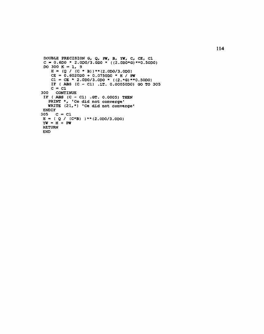
DOUBLE PRECISION G, Q, PW, B, YW, C, CE, CI C = O.6DO * 2,0D0/3 .OD0 * ( (2,0DO*G) **O.SODO) DO 300 K = 1, 9

H = ( Q / (C * B))**[2.OD0/3-ODO) CE = 0,602000 + 0.0750DO * H / PW Cl = CE * 2-OD0/3,ODO * ( ( 2 . * G ) **O.5ODO) IF ( ABS ( C - C1) -LT, 0.00050DO) GO TO 305 C = C1

300 CONTINOE IF ( ABS ( C - Cl) -GT. 0-0005) THEN

PRINT *, 'Ce did not converge1 WRITE (21,*) ICe did not converge1

ENDIF 305 C = C1 H = ( Q / (C*B) I * * (Z.ODO/3,ODO) Y W = H + P w RETURN END