A run-to-run framework for prandial insulin dosing ...jtc5/diabetes/run-to-run_real_life_uncertainty... · real-life uncertainty ... With the advent of home blood glucose monitoring

INTERNATIONAL JOURNAL OF ROBUST AND NONLINEAR CONTROLInt. J. Robust Nonlinear Control (in press)Published online in Wiley InterScience (www.interscience.wiley.com). DOI: 10.1002/rnc.1103

A run-to-run framework for prandial insulin dosing: handlingreal-life uncertainty

C. C. Palerm1,2,3, H. Zisser2, L. Jovanovic2,3 and F. J. Doyle III1,2,3,*,y

1Department of Chemical Engineering, University of California Santa Barbara, Santa Barbara, CA 93106-5080, U.S.A.2Sansum Diabetes Research Institute, 2219 Bath St., Santa Barbara, CA 93105, U.S.A.

3Biomolecular Science and Engineering Program, University of California Santa Barbara, Santa Barbara,CA 93106-9611, U.S.A.

SUMMARY

Individuals with type 1 diabetes require frequent adjustment of their insulin dose to maintain as near tonormal glycaemia as possible. This process is not only burdensome but also, for many, difficult to achieve.As a result, control algorithms to facilitate insulin dosage have been proposed, but have not beencompletely successful in normalizing glycaemia. Here we present a novel run-to-run control algorithm toadjust the meal-related insulin dose using only post-prandial blood glucose measurements. For each mealindependently, the insulin dose is adjusted based on the performance measure for the same meal theprevious day. A robustness analysis is performed which considers the sources of uncertainty typicallyencountered in clinical use. This shows that the system remains stable even with large uncertainty.Copyright # 2006 John Wiley & Sons, Ltd.

Received 8 November 2005; Accepted 1 August 2006

KEY WORDS: type 1 diabetes; run-to-run control; robustness; insulin dosing; biomedical control

1. INTRODUCTION

The Expert Committee on the Diagnosis and Classification of Diabetes Mellitus [1] definesdiabetes mellitus as a group of metabolic diseases which are characterized by hyperglycaemia(high levels of blood glucose). This hyperglycaemia results from defects in insulin secretion,insulin action, or both. Type 1 diabetes is caused by an absolute deficiency of insulin secretion,which is primarily due to b cell destruction. People with type 1 diabetes are prone to

*Correspondence to: F. J. Doyle III, Department of Chemical Engineering, University of California Santa Barbara,Santa Barbara, CA 93106-5080, U.S.A.yE-mail: [email protected]

Contract/grant sponsor: National Institutes of Health; contract/grant numbers: R01-DK068706, R01-DK068663

Copyright # 2006 John Wiley & Sons, Ltd.

ketoacidosis and fully depend on exogenous insulin. It is estimated that 17 million peopleworldwide had type 1 diabetes in 2000 [2, 3], with a clear rising trend in the worldwide incidenceof the disease of about 3% per year [4, 5].

The chronic hyperglycaemia in diabetes is associated with long-term complications due todamage, dysfunction and failure of various organs, especially the eyes, kidneys, nerves, heartand blood vessels. The main complications being heart disease, stroke, retinopathy,nephropathy and neuropathy. These can eventually lead to renal failure, blindness, amputationand other types of morbidity. Subjects with diabetes are at higher risk of cardiovascular disease,and face increased morbidity and mortality when critically ill.

The efficacy of intensive treatment in preventing diabetic complications has beenestablished by the Diabetes Control and Complications Trial (DCCT) [6] and the UnitedKingdom Prospective Diabetes Study (UKPDS) [7]. In both trials the treatment regimensthat reduced average glycosylated haemoglobin A1c (a clinical measure of glycaemiccontrol, which reflects average blood glucose levels over the preceding 2–3 months)to approximately 7% (normal range is 4–6%) were associated with fewer long-termmicrovascular complications. Recent evidence even suggests that these target levels might notbe low enough [8, 9].

Intensive treatment requires multiple (3 or more) daily injections of insulin or treatment withan insulin infusion pump. In any case, this tight control (i.e. as close to normal as possible)should be maintained for life in order to accrue the full benefits. Many factors influence theinsulin dose requirements over time, including weight, physical condition and stress levels. Dueto this, frequent blood glucose monitoring is required. Based on these measurements the insulindosage must be modified, dietary changes implemented (such as alteration in the timing,frequency and content of the meals), and activity and exercise patterns changed.

With the advent of home blood glucose monitoring technologies becoming available,physicians started to seek ways to use this information to fine-tune the therapeutic regimen.Among the first heuristic algorithms in the literature were those of Skyler et al. [10] andJovanovic and Peterson [11]. Both set heuristic rules based on practical experience; the maindifference between these two is that Skyler et al. [10] relies on pre-prandial blood glucosemeasurements exclusively, while Jovanovic and Peterson [11] uses pre- and post-prandialmeasurements to adjust the insulin dosing.

The algorithm proposed by Jovanovic and Peterson [11] was used as the basis to program apocket computer, which was tested in five type 1 diabetic subjects. They demonstrate thatcomputer-assisted insulin delivery decision making is feasible [12]. This computer program wasthen compared to the standard approach for new continuous subcutaneous insulin infusionpump users. Peterson et al. [13] found the approach to be feasible, although it did not fullynormalize blood glucose levels. Still, computer users achieved lower average blood glucose andA1c values over the course of the study.

Schiffrin et al. [14] programmed a portable computer to adjust dosing of short- andintermediate-acting insulin in a two-injection per day strategy, using pre-prandial blood glucosemeasurements. Even within the limitations of the therapy regimen used, they saw markedimprovements in glycaemic control when using the computer. Chiarelli et al. [15] compares thiscomputer method with a manual method; while they find no differences in glycaemic control,they did notice fewer instances of hypoglycaemia in the computer users. Peters et al. [16] adaptsthis algorithm and compares its effectiveness against manual adjustments, finding that metaboliccontrol and safety were comparable in both.

C. C. PALERM ET AL.

Copyright # 2006 John Wiley & Sons, Ltd. Int. J. Robust Nonlinear Control (in press)

DOI: 10.1002/rnc

Taking the heuristic algorithm of Skyler et al. [10] as their starting point, Beyer et al. [17]create their own algorithms; as the original, they use pre-prandial blood glucose measurements.In a clinical trial of 50 subjects they clearly show that the computer group did much better thanthe regular intensive treatment group [18].

In the work reviewed above, none of the computer algorithms make use of thenewer monomeric insulin formulations. Owens et al. [19] propose a run-to-run controlalgorithm to adjust the timing and dose of meal-related insulin boluses, taking advantageof these fast-acting insulin formulations. The basic assumption is that there is a sensoravailable from which frequent blood glucose measurements can be taken, and thusthe maximum and minimum blood glucose excursions in the prandial period can be determined.The feasibility of the algorithm was studied in a clinical setting, making some changes toallow for fingerstick blood glucose determinations at 60 and 90 min after the start of themeal in lieu of the maximum and minimum. Two-thirds of the subjects converged to, ormaintained, good glycaemic control, but the rest diverged in their responses due to variousfactors [20].

In this work, the algorithm is modified to overcome the difficulties encountered in clinicalpractice. The run-to-run formulation described here gives more flexibility to the subject, asblood glucose measurements are not required to be taken at specific times. In addition, formalrobustness is evaluated theoretically. In Section 2 the basis of the run-to-run algorithm ispresented, followed by the specific implementation for insulin dosing. Simulation results usingthis method are presented in Section 3, followed by a robustness analysis in Section 4 whichconsiders the expected sources of uncertainty.

2. RUN-TO-RUN ALGORITHM

The original formulation for the run-to-run control applied to insulin bolus dosing and timing isdescribed in Reference [19]. It is based on the application of a constraint control scheme in therun-to-run framework to optimize the operation of batch processes in the chemical industry[21, 22].

The general run-to-run control algorithm is as follows.

1. Parameterize the input profile for run k; ukðtÞ; asUðt; nkÞ: Also consider a sampled version,ck; of the output ykðtÞ; such that it has the same dimension as the controlled variablevector nk: Thus,

ck ¼ FðnkÞ ð1Þ

2. Choose an initial guess for nk (when k ¼ 1).3. Complete the run using the input ukðtÞ corresponding to nk: Determine ck from the

measurements ykðtÞ:4. Update the input parameters as

nkþ1 ¼ nk þ Kðcr � ckÞ ð2Þ

where K is an appropriate gain matrix and cr represents the reference valuesto be attained. Increment k for the next run, and repeat steps 3 and 4 untilconvergence.

RUN-TO-RUN FRAMEWORK FOR PRANDIAL INSULIN DOSING


DOI: 10.1002/rnc

In order to analyse the closed-loop system, a linearization of (1) is used:

ck ¼ Snk ð3Þ

S ¼@F

@nð4Þ

where S is the sensitivity matrix. Defining the error of the closed-loop system to be ek ¼ cr � ck;Equation (2) can be written as

nkþ1 ¼ nk þ Kek ð5Þ

Then at time kþ 1; and using (5) and (3), the error can be expressed as

ekþ1 ¼cr � ckþ1

¼cr � Snkþ1

¼cr � S nk þ Kekð Þ

¼cr � ck � SKek

¼ ðI � SKÞek ð6Þ

Thus, the stability and convergence of the algorithm depends on S and K :In the context of diabetes management, the natural day-to-day cycle is used as a ‘run’;

within this run, there are three separate meals (namely breakfast, lunch and dinner), forwhich an appropriate insulin bolus has to be determined. The objective is to minimizethe prandial glycaemic excursion without overdosing insulin. Thus, the manipulatedvariable, ukðtÞ; corresponds to the insulin profile, and the measurement profile, ykðtÞ;corresponds to glucose measurements. Time, t; is within a given day, while k denotes the day(run). Owens et al. [19] show, using an RGA analysis, that there is effectively no couplingbetween the meals; we also use this assumption, which we verify below, in the algorithmproposed in this paper.

There were two drawbacks to the original implementation when evaluated in a clinicalsetting. The first was the changing of the timing of the insulin bolus with respect to thestart of the meal. In several instances, this resulted in a bolus being administered in the middle ofa meal; at other times, the administration before the start of the meal was inconvenientto the subject, and was not adhered to. Furthermore, when using monomeric insulin, the timingof the bolus makes a negligible difference in the post-prandial profile when compared with theeffect of the dose. For these reasons it was decided to fix the timing to always coincide with thebeginning of the meal. The second drawback was the need for blood glucose determinations at60 and 90 min after the start of the meal; if the subject for some reason forgot to take either ofthem and was significantly off on the timing, then the algorithm was not able to correct for thefollowing day [20].

The main change in the algorithm is in the selection of the performance measure used. Tohave the flexibility of taking blood glucose measurements at different times, a fixed glucose levelcan no longer be used. Instead, an approximation of the slope of the glycaemic response is used.The only restrictions placed on the patient is that the first glucose measurement must be taken atleast 60 min after the start of the meal, and the second one be at least 30 min after the first, butnot more than 180 min after the start of the meal. These times are denoted, for each meal, as

C. C. PALERM ET AL.


DOI: 10.1002/rnc

TB1; TB2

; TL1; TL2

; TD1; TD2

: Then, the sampled output vector is

ck ¼

GðTB1Þ � GðTB2

Þ

GðTL1Þ � GðTL2

Þ

GðTD1Þ � GðTD2

Þ

26664

37775 ð7Þ

As the times can change from one meal to the next, and from run to run, a reference value isrequired that is normalized with respect to time. This reference is defined in terms of units ofglucose per minute for each meal, cr

0; and then scaled by the actual time between the twomeasurements. This is expressed as

cr ¼ cr08

TB2� TB1

TL2� TL1

TD2� TD1

266664

377775 ð8Þ

where 8 denotes the Hadamard (elementwise) product.The manipulated variable nk is simply the dose of insulin (per gram of carbohydrate

in the meal) corresponding to each meal of day k; nk ¼ ½QB QL QD�T: The controllergain, K ; is set according to the desired speed of response as well as the insulin sensitivity of thepatient.

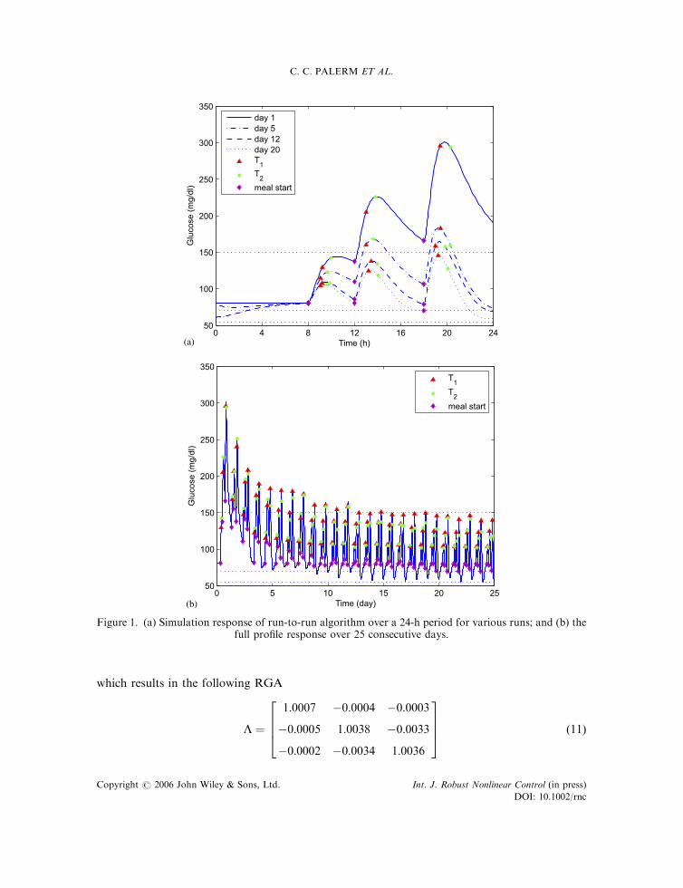
The rationale for this performance measure is explained by the blood glucose response seenfor different doses. For a bolus that is correctly dosed, the peak glucose excursion is expected tobe around 60 min; and to drop from that point on until it reaches the basal level. If the bolus isunder-dosed, this moves the peak into the future. Thus, if the bolus is under-dosed, thedifference in blood glucose levels between the first and second measurements will be negative, orpositive but very small. As the dose approaches the ideal level, this difference will increase. Thisis all illustrated in Figure 1(a).

Using this performance measure, the steady state gain and the relative gain array can becalculated. If all perturbations to calculate the response are done starting from steady state, thegain matrix is

KSS ¼

7:02 0 0

�0:95 6:55 0

�0:49 �1:15 5:57

266664

377775 ð9Þ

given that the upper-triangular is all zeros, the RGA is the identity matrix, showing no coupling.If for each perturbation the final conditions are used as the initial point for the following day,then the gain matrix is

KSS ¼

6:93 �0:02 �0:02

�0:98 6:42 �0:10

�0:50 �1:16 5:55

266664

377775 ð10Þ



DOI: 10.1002/rnc

which results in the following RGA

L ¼

1:0007 �0:0004 �0:0003

�0:0005 1:0038 �0:0033

�0:0002 �0:0034 1:0036

2664

3775 ð11Þ

0 4 8 12 16 20 2450

100

150

200

250

300

350

Time (h)

Glu

co

se

(m

g/d

l)

day 1

day 5

day 12

day 20

T1

T2

meal start

0 5 10 15 20 2550

100

150

200

250

300

350

Time (day)

Glu

co

se

(m

g/d

l)

T1

T2

meal start

(a)

(b)

Figure 1. (a) Simulation response of run-to-run algorithm over a 24-h period for various runs; and (b) thefull profile response over 25 consecutive days.

C. C. PALERM ET AL.


DOI: 10.1002/rnc

which although not exactly the identity matrix, it still shows there is no significant coupling.Given that the performance measure is a relative value it makes sense intuitively that this wouldbe the case, as any remaining effect of a previous insulin bolus will affect both glucosemeasurements by practically the same extent.

3. SIMULATION RESULTS

There are several published models of glucose and insulin dynamics in the literature. For thisparticular study the one published by Hovorka et al. [23] is used, replacing the subcutaneousinsulin infusion model with the one described in Reference [24]. The model captures not only thedynamics of glucose and insulin, but also the absorption of insulin from a subcutaneous delivery(as is the case with insulin infusion pumps), and the appearance of glucose in plasma from amixed meal.

For each day, the simulation has the meals at 8:00, 12:00 and 18:00 h; with a carbohydratecontent of 20, 40 and 70 g; respectively. For each day and meal, the time points at which bloodglucose measurements are taken are selected randomly (using a uniform distribution); the firstone can take place from 60 to 90 min after the start of the meal, the second one follows 30 to60 min later.

The reference drop in blood glucose (per minute), was selected for each meal separately,considering the typical amount of carbohydrate consumed in each meal as the main guideline. Inthis case, cr

0 ¼ ½0:058 0:104 0:30�T: The controller gain is set at K ¼ 0:001; and is scaled by 0.5, 2or 3 for subjects with higher or lower insulin sensitivities. The amount of the insulin bolus isrounded to the nearest 0.1 IU of insulin, which is the resolution of most commercially availableinfusion pumps.

The initial guess for the insulin requirement for each meal is set at an insulin to carbohydrateratio of 1:33 (a more typical value is around 1:10). Thus, the starting dose gives much less insulinthan is actually required for the first run (k ¼ 0). Figure 1(b) shows the simulation for 25 days,with Figure 1(a) highlighting a couple of days. The dotted lines show the desired bounds for theblood glucose excursions; note that we are more aggressive in keeping blood glucose below150 mg=dl than preventing it from going below 70 mg=dl:

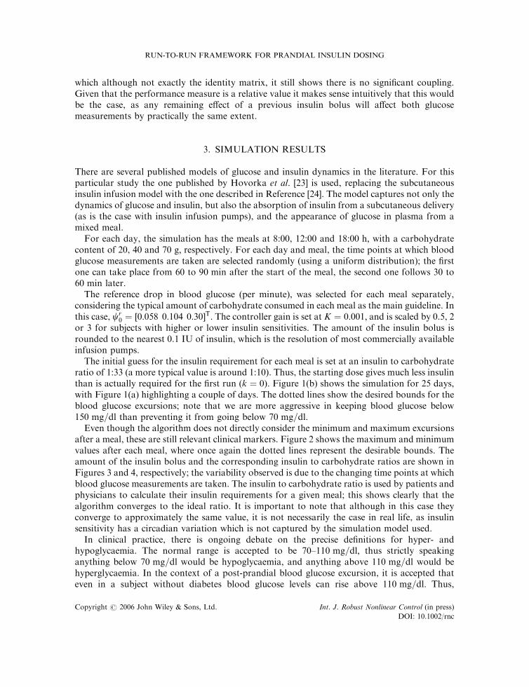
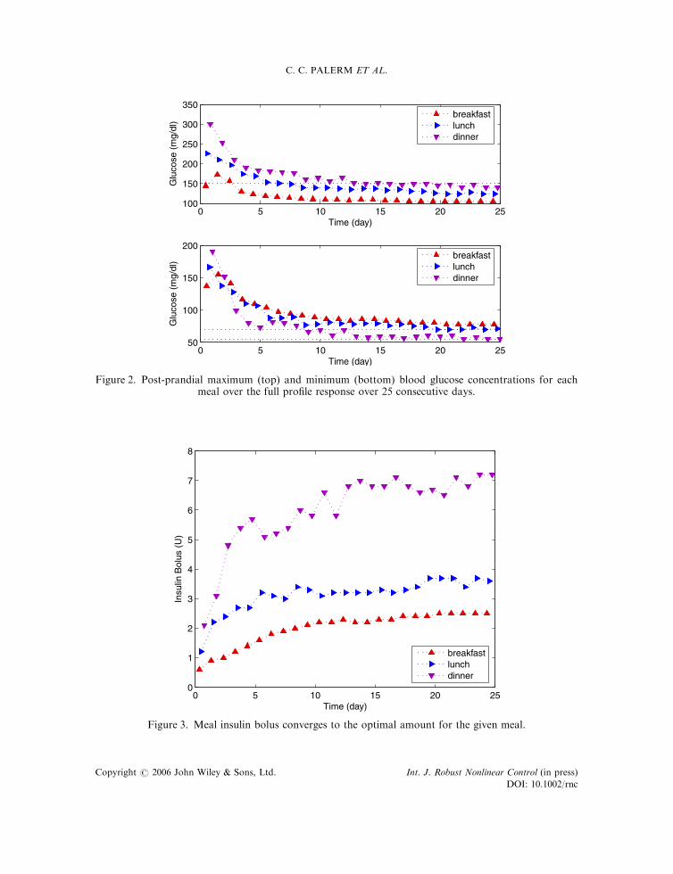
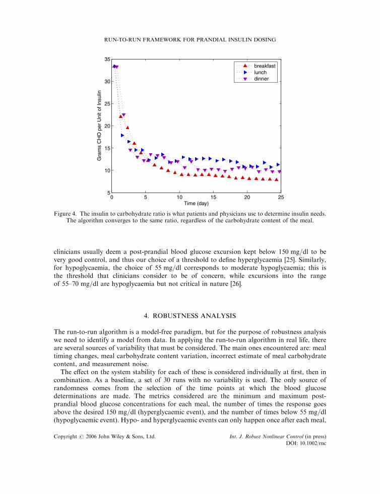
Even though the algorithm does not directly consider the minimum and maximum excursionsafter a meal, these are still relevant clinical markers. Figure 2 shows the maximum and minimumvalues after each meal, where once again the dotted lines represent the desirable bounds. Theamount of the insulin bolus and the corresponding insulin to carbohydrate ratios are shown inFigures 3 and 4, respectively; the variability observed is due to the changing time points at whichblood glucose measurements are taken. The insulin to carbohydrate ratio is used by patients andphysicians to calculate their insulin requirements for a given meal; this shows clearly that thealgorithm converges to the ideal ratio. It is important to note that although in this case theyconverge to approximately the same value, it is not necessarily the case in real life, as insulinsensitivity has a circadian variation which is not captured by the simulation model used.

In clinical practice, there is ongoing debate on the precise definitions for hyper- andhypoglycaemia. The normal range is accepted to be 70–110 mg=dl; thus strictly speakinganything below 70 mg=dl would be hypoglycaemia, and anything above 110 mg=dl would behyperglycaemia. In the context of a post-prandial blood glucose excursion, it is accepted thateven in a subject without diabetes blood glucose levels can rise above 110 mg=dl: Thus,



DOI: 10.1002/rnc

0 5 10 15 20 25100

150

200

250

300

350

Time (day)

Glu

cose

(m

g/dl

)

0 5 10 15 20 2550

100

150

200

Time (day)

Glu

cose

(m

g/dl

)

breakfastlunchdinner


Figure 2. Post-prandial maximum (top) and minimum (bottom) blood glucose concentrations for eachmeal over the full profile response over 25 consecutive days.

0 5 10 15 20 250

1

2

3

4

5

6

7

8

Time (day)

Insu

lin B

olus

(U

)


Figure 3. Meal insulin bolus converges to the optimal amount for the given meal.

C. C. PALERM ET AL.


DOI: 10.1002/rnc

clinicians usually deem a post-prandial blood glucose excursion kept below 150 mg=dl to bevery good control, and thus our choice of a threshold to define hyperglycaemia [25]. Similarly,for hypoglycaemia, the choice of 55 mg=dl corresponds to moderate hypoglycaemia; this isthe threshold that clinicians consider to be of concern, while excursions into the rangeof 55–70 mg=dl are hypoglycaemia but not critical in nature [26].

4. ROBUSTNESS ANALYSIS

The run-to-run algorithm is a model-free paradigm, but for the purpose of robustness analysiswe need to identify a model from data. In applying the run-to-run algorithm in real life, thereare several sources of variability that must be considered. The main ones encountered are: mealtiming changes, meal carbohydrate content variation, incorrect estimate of meal carbohydratecontent, and measurement noise.

The effect on the system stability for each of these is considered individually at first, then incombination. As a baseline, a set of 30 runs with no variability is used. The only source ofrandomness comes from the selection of the time points at which the blood glucosedeterminations are made. The metrics considered are the minimum and maximum post-prandial blood glucose concentrations for each meal, the number of times the response goesabove the desired 150 mg=dl (hyperglycaemic event), and the number of times below 55 mg=dl(hypoglycaemic event). Hypo- and hyperglycaemic events can only happen once after each meal,

0 5 10 15 20 255

10

15

20

25

30

35

Time (day)

Gra

ms

CH

O p

er U

nit o

f Ins

ulin


Figure 4. The insulin to carbohydrate ratio is what patients and physicians use to determine insulin needs.The algorithm converges to the same ratio, regardless of the carbohydrate content of the meal.



DOI: 10.1002/rnc

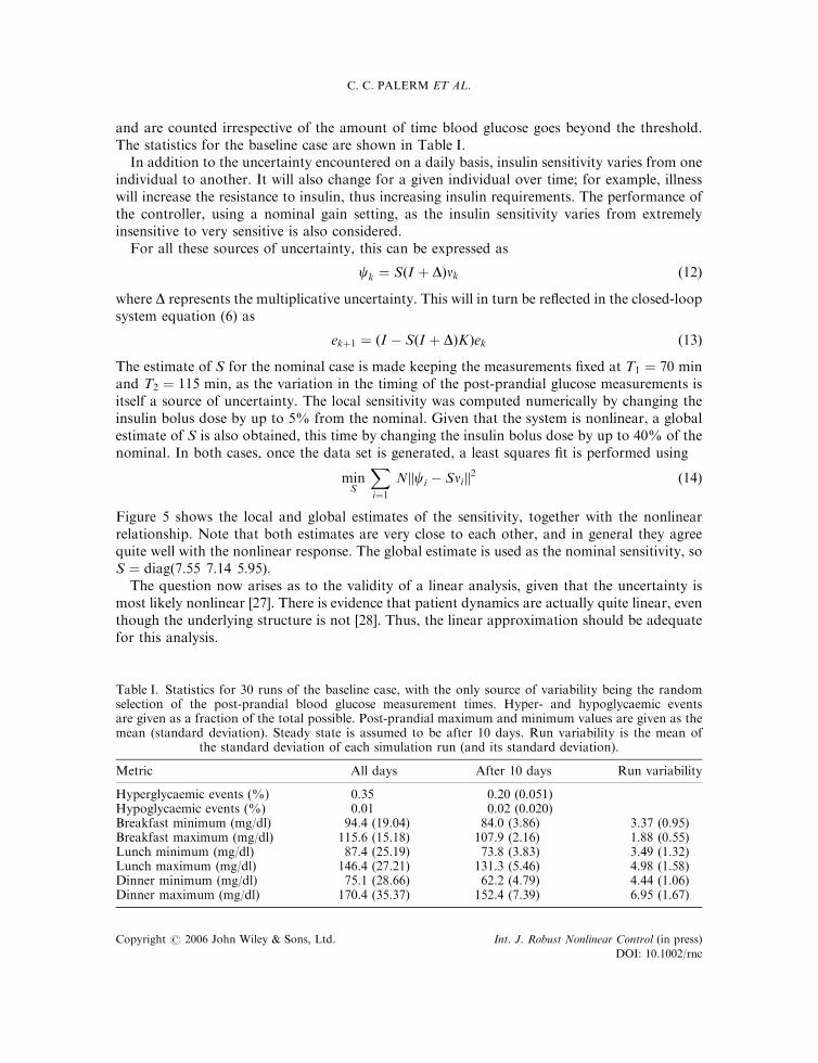
and are counted irrespective of the amount of time blood glucose goes beyond the threshold.The statistics for the baseline case are shown in Table I.

In addition to the uncertainty encountered on a daily basis, insulin sensitivity varies from oneindividual to another. It will also change for a given individual over time; for example, illnesswill increase the resistance to insulin, thus increasing insulin requirements. The performance ofthe controller, using a nominal gain setting, as the insulin sensitivity varies from extremelyinsensitive to very sensitive is also considered.

For all these sources of uncertainty, this can be expressed as

ck ¼ SðI þ DÞnk ð12Þ

where D represents the multiplicative uncertainty. This will in turn be reflected in the closed-loopsystem equation (6) as

ekþ1 ¼ ðI � SðI þ DÞKÞek ð13Þ

The estimate of S for the nominal case is made keeping the measurements fixed at T1 ¼ 70 minand T2 ¼ 115 min; as the variation in the timing of the post-prandial glucose measurements isitself a source of uncertainty. The local sensitivity was computed numerically by changing theinsulin bolus dose by up to 5% from the nominal. Given that the system is nonlinear, a globalestimate of S is also obtained, this time by changing the insulin bolus dose by up to 40% of thenominal. In both cases, once the data set is generated, a least squares fit is performed using

minS

Xi¼1

Njjci � Sni jj2 ð14Þ

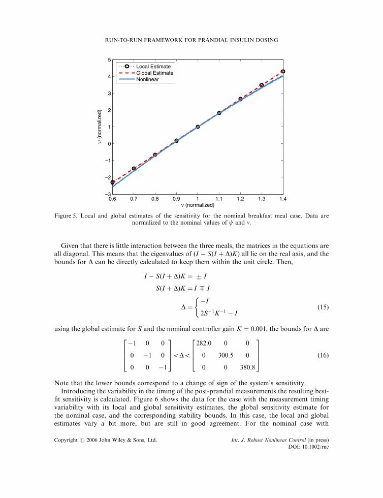
Figure 5 shows the local and global estimates of the sensitivity, together with the nonlinearrelationship. Note that both estimates are very close to each other, and in general they agreequite well with the nonlinear response. The global estimate is used as the nominal sensitivity, soS ¼ diagð7:55 7:14 5:95Þ:

The question now arises as to the validity of a linear analysis, given that the uncertainty ismost likely nonlinear [27]. There is evidence that patient dynamics are actually quite linear, eventhough the underlying structure is not [28]. Thus, the linear approximation should be adequatefor this analysis.

Table I. Statistics for 30 runs of the baseline case, with the only source of variability being the randomselection of the post-prandial blood glucose measurement times. Hyper- and hypoglycaemic eventsare given as a fraction of the total possible. Post-prandial maximum and minimum values are given as themean (standard deviation). Steady state is assumed to be after 10 days. Run variability is the mean of

the standard deviation of each simulation run (and its standard deviation).

Metric All days After 10 days Run variability

Hyperglycaemic events (%) 0.35 0.20 (0.051)Hypoglycaemic events (%) 0.01 0.02 (0.020)Breakfast minimum (mg/dl) 94.4 (19.04) 84.0 (3.86) 3.37 (0.95)Breakfast maximum (mg/dl) 115.6 (15.18) 107.9 (2.16) 1.88 (0.55)Lunch minimum (mg/dl) 87.4 (25.19) 73.8 (3.83) 3.49 (1.32)Lunch maximum (mg/dl) 146.4 (27.21) 131.3 (5.46) 4.98 (1.58)Dinner minimum (mg/dl) 75.1 (28.66) 62.2 (4.79) 4.44 (1.06)Dinner maximum (mg/dl) 170.4 (35.37) 152.4 (7.39) 6.95 (1.67)

C. C. PALERM ET AL.


DOI: 10.1002/rnc

Given that there is little interaction between the three meals, the matrices in the equations areall diagonal. This means that the eigenvalues of ðI � SðI þ DÞKÞ all lie on the real axis, and thebounds for D can be directly calculated to keep them within the unit circle. Then,

I � SðI þ DÞK ¼ � I

SðI þ DÞK ¼ I � I

D ¼�I

2S�1K�1 � I

(ð15Þ

using the global estimate for S and the nominal controller gain K ¼ 0:001; the bounds for D are

�1 0 0

0 �1 0

0 0 �1

2664

37755D5

282:0 0 0

0 300:5 0

0 0 380:8

2664

3775 ð16Þ

Note that the lower bounds correspond to a change of sign of the system’s sensitivity.Introducing the variability in the timing of the post-prandial measurements the resulting best-

fit sensitivity is calculated. Figure 6 shows the data for the case with the measurement timingvariability with its local and global sensitivity estimates, the global sensitivity estimate forthe nominal case, and the corresponding stability bounds. In this case, the local and globalestimates vary a bit more, but are still in good agreement. For the nominal case with

0.6 0.7 0.8 0.9 1 1.1 1.2 1.3 1.4

0

1

2

3

4

5

ν (normalized)

ψ (

norm

aliz

ed)

Local EstimateGlobal EstimateNonlinear

Figure 5. Local and global estimates of the sensitivity for the nominal breakfast meal case. Data arenormalized to the nominal values of c and n:



DOI: 10.1002/rnc

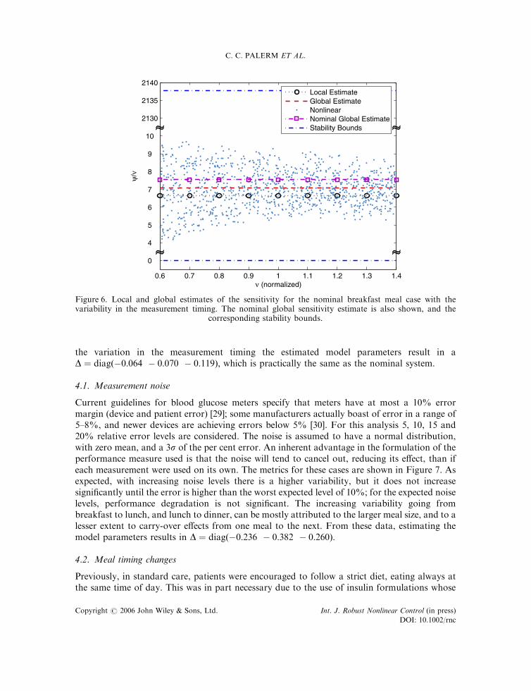
the variation in the measurement timing the estimated model parameters result in aD ¼ diagð�0:064 � 0:070 � 0:119Þ; which is practically the same as the nominal system.

4.1. Measurement noise

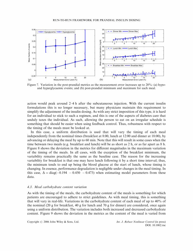
Current guidelines for blood glucose meters specify that meters have at most a 10% errormargin (device and patient error) [29]; some manufacturers actually boast of error in a range of5–8%, and newer devices are achieving errors below 5% [30]. For this analysis 5, 10, 15 and20% relative error levels are considered. The noise is assumed to have a normal distribution,with zero mean, and a 3s of the per cent error. An inherent advantage in the formulation of theperformance measure used is that the noise will tend to cancel out, reducing its effect, than ifeach measurement were used on its own. The metrics for these cases are shown in Figure 7. Asexpected, with increasing noise levels there is a higher variability, but it does not increasesignificantly until the error is higher than the worst expected level of 10%; for the expected noiselevels, performance degradation is not significant. The increasing variability going frombreakfast to lunch, and lunch to dinner, can be mostly attributed to the larger meal size, and to alesser extent to carry-over effects from one meal to the next. From these data, estimating themodel parameters results in D ¼ diagð�0:236 � 0:382 � 0:260Þ:

4.2. Meal timing changes

Previously, in standard care, patients were encouraged to follow a strict diet, eating always atthe same time of day. This was in part necessary due to the use of insulin formulations whose

0.6 0.7 0.8 0.9 1 1.1 1.2 1.3 1.4

0

4

5

6

7

8

9

10

2130

2135

2140

ν (normalized)

ψ/ν

~~ ~~

~~ ~~

Local EstimateGlobal EstimateNonlinearNominal Global EstimateStability Bounds

Figure 6. Local and global estimates of the sensitivity for the nominal breakfast meal case with thevariability in the measurement timing. The nominal global sensitivity estimate is also shown, and the

corresponding stability bounds.

C. C. PALERM ET AL.


DOI: 10.1002/rnc

action would peak around 2–4 h after the subcutaneous injection. With the current insulinformulations this is no longer necessary, but many physicians maintain this requirement tosimplify the adjustment of the insulin dosing. As with any strict imposition of this type, it is hardfor an individual to stick to such a regimen, and this is one of the aspects of diabetes care thatunduly taxes the individual. As such, allowing the person to eat on an irregular schedule issomething that should be easier when using feedback control. Thus, robustness with respect tothe timing of the meals must be looked at.

In this case, a uniform distribution is used that will vary the timing of each mealindependently from the nominal times (breakfast at 8:00, lunch at 12:00 and dinner at 18:00), byadvancing or delaying the meal by up to 60 min:Note that this will result in some cases when thetime between two meals (e.g. breakfast and lunch) will be as short as 2 h; or as far apart as 8 h:Figure 8 shows the deviation in the metrics for different magnitudes in the maximum variationof the timing of the meals. In all cases, with the exception of the breakfast minimum, thevariability remains practically the same as the baseline case. The reason for the increasingvariability for breakfast is that one may have lunch following it by a short time interval; thus,the minimum tends to end up being the blood glucose at the start of lunch, whose timing ischanging. In essence, performance degradation is negligible under changes in the meal timing. Inthis case, D ¼ diagð�0:194 � 0:450 � 0:473Þ when estimating model parameters from thesedata.

4.3. Meal carbohydrate content variation

As with the timing of the meals, the carbohydrate content of the meals is something for whichpatients are encouraged to adhere to strict guidelines. As with meal timing, this is somethingthat will vary in real-life. Variations in the carbohydrate content of each meal of up to 40% ofthe nominal (20 g for breakfast, 40 g for lunch and 70 g for dinner) are considered, once againusing a uniform distribution. The variation includes both increased and decreased carbohydratecontent. Figure 9 shows the deviation in the metrics as the content of the meal is varied from

0 5 10 15 20

0

0.05

0.1

0.15

0.2

0.25

0.3

0.35

Measurement Error Level (%)

Mea

n fr

actio

n of

eve

nts

Hypoglycemia Hyperglycemia

0 5 10 15 200

10

20

30

Measurement Error Level (%)

[ ] [ ] [ ] [ ] [ ]

0 5 10 15 200

10

20

30

[ ] [ ] [ ] [ ] [ ]

Mea

n st

anda

rd d

evia

tion

(mg/

dl)

0 5 10 15 200

10

20

30

[ ] [ ] [ ] [ ] [ ]

Dinner Min Dinner Max

Lunch Min Lunch Max

Breakfast Min Breakfast Max

(a) (b)

Figure 7. Variation in the post-prandial metrics as the measurement error increases up to 20%: (a) hypo-and hyperglycaemic events; and (b) post-prandial minimum and maximum for each meal.



DOI: 10.1002/rnc

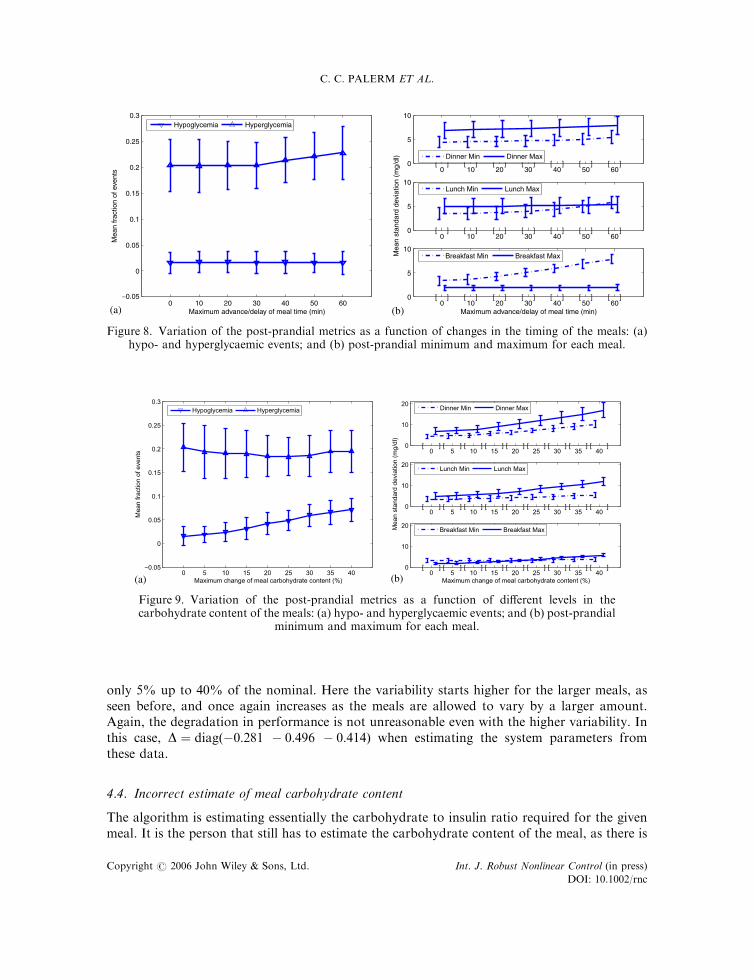
only 5% up to 40% of the nominal. Here the variability starts higher for the larger meals, asseen before, and once again increases as the meals are allowed to vary by a larger amount.Again, the degradation in performance is not unreasonable even with the higher variability. Inthis case, D ¼ diagð�0:281 � 0:496 � 0:414Þ when estimating the system parameters fromthese data.

4.4. Incorrect estimate of meal carbohydrate content

The algorithm is estimating essentially the carbohydrate to insulin ratio required for the givenmeal. It is the person that still has to estimate the carbohydrate content of the meal, as there is

0 10 20 30 40 50 60

0

0.05

−0.05

0.1

0.15

0.2

0.25

0.3

Maximum advance/delay of meal time (min)

Mea

n fr

actio

n of

eve

nts


0 10 20 30 40 50 600

5

10

Maximum advance/delay of meal time (min)

[ ] [ ] [ ] [ ] [ ] [ ] [ ]

0 10 20 30 40 50 600

5

10

[ ] [ ] [ ] [ ] [ ] [ ] [ ]

Mea

n st

anda

rd d

evia

tion

(mg/

dl)

0 10 20 30 40 50 600

5

10

[ ] [ ] [ ] [ ] [ ] [ ] [ ]Dinner Min Dinner Max

Lunch Min Lunch Max


(a) (b)

Figure 8. Variation of the post-prandial metrics as a function of changes in the timing of the meals: (a)hypo- and hyperglycaemic events; and (b) post-prandial minimum and maximum for each meal.

0 5 10 15 20 25 30 35 40

0

0.05

0.1

0.15

0.2

0.25

0.3

Maximum change of meal carbohydrate content (%)

Me

an

fra

ctio

n o

f e

ve

nts


0 5 10 15 20 25 30 35 400

10

20

Maximum change of meal carbohydrate content (%)

[ ] [ ] [ ] [ ] [ ] [ ] [ ] [ ] [ ]

0 5 10 15 20 25 30 35 400

10

20

[ ] [ ] [ ] [ ] [ ] [ ] [ ] [ ] [ ]

Me

an

sta

nd

ard

de

via

tio

n (

mg

/dl)

0 5 10 15 20 25 30 35 400

10

20

[ ] [ ] [ ] [ ] [ ] [ ] [ ] [ ] [ ]


Lunch Min Lunch Max


(a) (b)

Figure 9. Variation of the post-prandial metrics as a function of different levels in thecarbohydrate content of the meals: (a) hypo- and hyperglycaemic events; and (b) post-prandial

minimum and maximum for each meal.

C. C. PALERM ET AL.


DOI: 10.1002/rnc

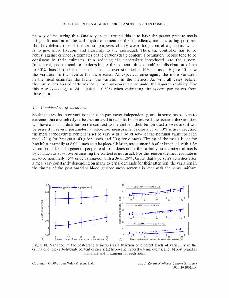
no way of measuring this. One way to get around this is to have the person prepare mealsusing information of the carbohydrate content of the ingredients, and measuring portions.But this defeats one of the central purposes of any closed-loop control algorithm, whichis to give more freedom and flexibility to the individual. Thus, the controller has to berobust against erroneous estimates of the carbohydrate content. Fortunately, people tend to beconsistent in their estimates, thus reducing the uncertainty introduced into the system.In general, people tend to underestimate the content, thus a uniform distribution of upto 40%, biased so that the most a meal is overestimated is 10%, is used. Figure 10 showthe variation in the metrics for these cases. As expected, once again, the more variationin the meal estimates the higher the variation in the metrics. As with all cases before,the controller’s loss of performance is not unreasonable even under the largest variability. Forthis case D ¼ diagð�0:184 � 0:415 � 0:395Þ when estimating the system parameters fromthese data.

4.5. Combined set of variations

So far the results show variations in each parameter independently, and in some cases taken toextremes that are unlikely to be encountered in real life. In a more realistic scenario the variationwill have a normal distribution (in contrast to the uniform distribution used above), and it willbe present in several parameters at once. For measurement noise a 3s of 10% is assumed, andthe meal carbohydrate content is set to vary with a 3s of 40% of the nominal value for eachmeal (20 g for breakfast, 40 g for lunch and 70 g for dinner). Timing of the meals is set forbreakfast normally at 8:00, lunch to take place 5 h later, and dinner 6 h after lunch; all with a 3svariation of 1:5 h: In general, people tend to underestimate the carbohydrate content of mealsby as much as 30%; overestimating the content is not usual. For this reason the meal estimate isset to be nominally 15% underestimated, with a 3s of 20%. Given that a person’s activities aftera meal vary constantly depending on many external demands for their attention, the variation inthe timing of the post-prandial blood glucose measurements is kept with the same uniform

0 10 20 30 40

0

0.05

0.1

0.15

0.2

0.25

0.3

Maximum change of meal carbohydrate content estimate (%)

Mea

n fr

actio

n of

eve

nts


0 10 20 30 400

10

20

Maximum change of meal carbohydrate content estimate (%)

[ ] [ ] [ ] [ ] [ ]

0 10 20 30 400

10

20

[ ] [ ] [ ] [ ] [ ]

Mea

n st

anda

rd d

evia

tion

(mg/

dl)

0 10 20 30 400

10

20

[ ] [ ] [ ] [ ] [ ]


Lunch Min Lunch Max


(a) (b)

Figure 10. Variation of the post-prandial metrics as a function of different levels of variability in theestimates of the carbohydrate content of meals: (a) hypo- and hyperglycaemic events; and (b) post-prandial

minimum and maximum for each meal.



DOI: 10.1002/rnc

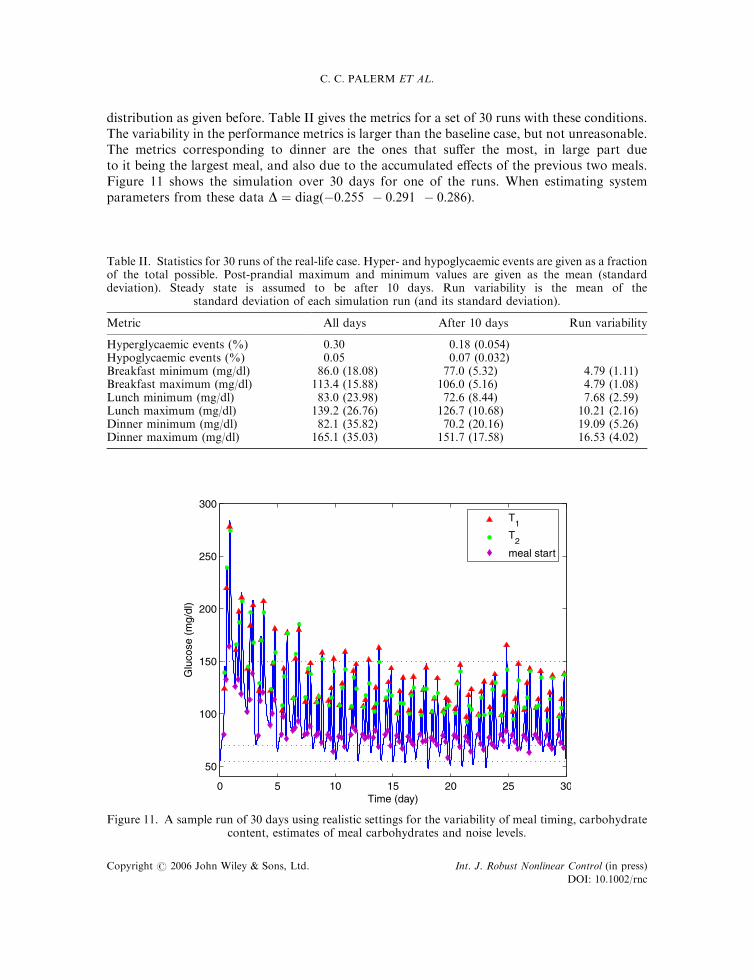
distribution as given before. Table II gives the metrics for a set of 30 runs with these conditions.The variability in the performance metrics is larger than the baseline case, but not unreasonable.The metrics corresponding to dinner are the ones that suffer the most, in large part dueto it being the largest meal, and also due to the accumulated effects of the previous two meals.Figure 11 shows the simulation over 30 days for one of the runs. When estimating systemparameters from these data D ¼ diagð�0:255 � 0:291 � 0:286Þ:

Table II. Statistics for 30 runs of the real-life case. Hyper- and hypoglycaemic events are given as a fractionof the total possible. Post-prandial maximum and minimum values are given as the mean (standarddeviation). Steady state is assumed to be after 10 days. Run variability is the mean of the

standard deviation of each simulation run (and its standard deviation).

Metric All days After 10 days Run variability

Hyperglycaemic events (%) 0.30 0.18 (0.054)Hypoglycaemic events (%) 0.05 0.07 (0.032)Breakfast minimum (mg/dl) 86.0 (18.08) 77.0 (5.32) 4.79 (1.11)Breakfast maximum (mg/dl) 113.4 (15.88) 106.0 (5.16) 4.79 (1.08)Lunch minimum (mg/dl) 83.0 (23.98) 72.6 (8.44) 7.68 (2.59)Lunch maximum (mg/dl) 139.2 (26.76) 126.7 (10.68) 10.21 (2.16)Dinner minimum (mg/dl) 82.1 (35.82) 70.2 (20.16) 19.09 (5.26)Dinner maximum (mg/dl) 165.1 (35.03) 151.7 (17.58) 16.53 (4.02)

0 5 10 15 20 25 30

50

100

150

200

250

300

Time (day)

Glu

cose

(m

g/dl

)

T1

T2

meal start

Figure 11. A sample run of 30 days using realistic settings for the variability of meal timing, carbohydratecontent, estimates of meal carbohydrates and noise levels.

C. C. PALERM ET AL.


DOI: 10.1002/rnc

4.6. Insulin sensitivity

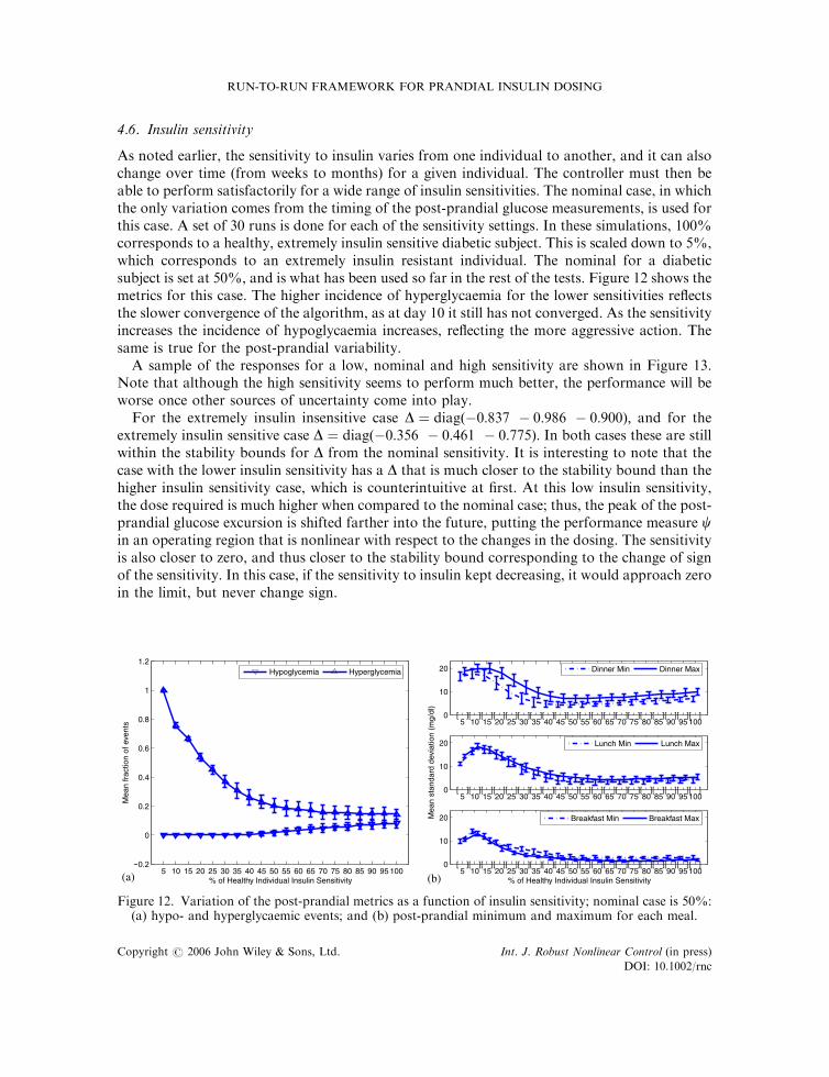
As noted earlier, the sensitivity to insulin varies from one individual to another, and it can alsochange over time (from weeks to months) for a given individual. The controller must then beable to perform satisfactorily for a wide range of insulin sensitivities. The nominal case, in whichthe only variation comes from the timing of the post-prandial glucose measurements, is used forthis case. A set of 30 runs is done for each of the sensitivity settings. In these simulations, 100%corresponds to a healthy, extremely insulin sensitive diabetic subject. This is scaled down to 5%,which corresponds to an extremely insulin resistant individual. The nominal for a diabeticsubject is set at 50%, and is what has been used so far in the rest of the tests. Figure 12 shows themetrics for this case. The higher incidence of hyperglycaemia for the lower sensitivities reflectsthe slower convergence of the algorithm, as at day 10 it still has not converged. As the sensitivityincreases the incidence of hypoglycaemia increases, reflecting the more aggressive action. Thesame is true for the post-prandial variability.

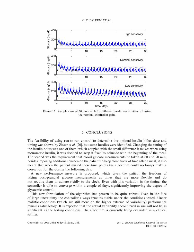
A sample of the responses for a low, nominal and high sensitivity are shown in Figure 13.Note that although the high sensitivity seems to perform much better, the performance will beworse once other sources of uncertainty come into play.

For the extremely insulin insensitive case D ¼ diagð�0:837 � 0:986 � 0:900Þ; and for theextremely insulin sensitive case D ¼ diagð�0:356 � 0:461 � 0:775Þ: In both cases these are stillwithin the stability bounds for D from the nominal sensitivity. It is interesting to note that thecase with the lower insulin sensitivity has a D that is much closer to the stability bound than thehigher insulin sensitivity case, which is counterintuitive at first. At this low insulin sensitivity,the dose required is much higher when compared to the nominal case; thus, the peak of the post-prandial glucose excursion is shifted farther into the future, putting the performance measure cin an operating region that is nonlinear with respect to the changes in the dosing. The sensitivityis also closer to zero, and thus closer to the stability bound corresponding to the change of signof the sensitivity. In this case, if the sensitivity to insulin kept decreasing, it would approach zeroin the limit, but never change sign.

5 10 15 20 25 30 35 40 45 50 55 60 65 70 75 80 85 90 95 100

0

0.2

0.4

0.6

0.8

1

1.2

% of Healthy Individual Insulin Sensitivity

Mea

n fr

actio

n of

eve

nts


5 10 15 20 25 30 35 40 45 50 55 60 65 70 75 80 85 90 95 1000

10

20

% of Healthy Individual Insulin Sensitivity

[ ][ ][ ][ ][ ][ ][ ][ ][ ][ ][ ][ ][ ][ ][ ][ ][ ][ ][ ][ ]

5 10 15 20 25 30 35 40 45 50 55 60 65 70 75 80 85 90 95 1000

10

20

[ ][ ][ ][ ][ ][ ][ ][ ][ ][ ][ ][ ][ ][ ][ ][ ][ ][ ][ ][ ]

Mea

n st

anda

rd d

evia

tion

(mg/

dl)

5 10 15 20 25 30 35 40 45 50 55 60 65 70 75 80 85 90 95 1000

10

20

[ ][ ][ ][ ][ ][ ][ ][ ][ ][ ][ ][ ][ ][ ][ ][ ][ ][ ][ ][ ]


Lunch Min Lunch Max


(a) (b)

Figure 12. Variation of the post-prandial metrics as a function of insulin sensitivity; nominal case is 50%:(a) hypo- and hyperglycaemic events; and (b) post-prandial minimum and maximum for each meal.



DOI: 10.1002/rnc

5. CONCLUSIONS

The feasibility of using run-to-run control to determine the optimal insulin bolus dose andtiming was shown by Zisser et al. [20], but some hurdles were identified. Changing the timing ofthe insulin bolus was one of them, which coupled with the small difference it makes when usingmonomeric insulin, it was decided to keep it fixed to coincide with the beginning of the meal.The second was the requirement that blood glucose measurements be taken at 60 and 90 min;besides imposing additional burden on the patient to keep close track of time after a meal, it alsomeant that when the patient missed these time points the algorithm could no longer make acorrection for the dosing the following day.

A new performance measure is proposed, which gives the patient the freedom oftaking post-prandial glucose measurements at times that are more flexible and donot require them to adhere rigidly to the clock. Even with this variation in the timing, thecontroller is able to converge within a couple of days, significantly improving the degree ofglycaemic control.

This new formulation of the algorithm has proven to be quite robust. Even in the faceof large uncertainty the controller always remains stable under the conditions tested. Underrealistic conditions (which are still more on the higher extreme of variability) performanceremains satisfactory. It is expected that the actual variability encountered in use will not be assignificant as the testing conditions. The algorithm is currently being evaluated in a clinicalsetting.

0 5 10 15 20 25 300

200

400

Glu

cose

(m

g/dl

)

High sensitivity

0 5 10 15 20 25 300

200

400

Glu

cose

(m

g/dl

)

Nominal sensitivity

0 5 10 15 20 25 300

200

400

Time (day)

Glu

cose

(m

g/dl

)

Low sensitivity

Figure 13. Sample runs of 30 days each for different insulin sensitivities, all usingthe nominal controller gain.

C. C. PALERM ET AL.


DOI: 10.1002/rnc

REFERENCES

1. Expert Committee on the Diagnosis and Classification of Diabetes Mellitus. Report of the expert committee on thediagnosis and classification of diabetes mellitus. Diabetes Care 2003; 26(s1):s5–s20.

2. Wild S, Roglic G, Green A, Sicree R, King H. Global prevalence of diabetes: estimates for the year 2000 andprojections for 2030. Diabetes Care 2004; 27(5):1047–1053.

3. Eiselein L, Schwartz HJ, Rutledge JC. The challenge of type 1 diabetes mellitus. ILAR Journal 2004; 45(3):231–236.

4. Gale EAM. Spring harvest? Reflections on the rise of type 1 diabetes. Diabetologia 2005; 48(12):2445–2450.doi:10.1007/s00125-005-0028-z.

5. Daneman D. Type 1 diabetes. Lancet 2006; 367(9513):847–858. doi:10.1016/S0140-6736(06)68341-4.6. Diabetes Control and Complications Trials Research Group. The effect of intensive treatment of diabetes on the

development and progression of long-term complications in insulin-dependent diabetes mellitus. New EnglandJournal of Medicine 1993; 329:977–986.

7. UK Prospective Diabetes Study Group. Intensive blood-glucose control with sulphonylureas or insulin comparedwith conventional treatment and risk of complications in patients with type 2 diabetes (UKPDS 33). Lancet 1998;352:837–853.

8. Khaw K, Wareham N, Luben R, Bingham S, Oakes S, Welch A, Day N. Glycated haemoglobin, diabetes, andmortality in men in Norfolk cohort of European Prospective Investigation of Cancer and Nutrition (EPIC-Norfolk).British Medical Journal 2001; 322(7277):15–18.

9. Muntner P, Wildman RP, Reynolds K, Desalvo KB, Chen J, Fonseca V. Relationship between HbA1c level andperipheral arterial disease. Diabetes Care 2005; 28(8):1981–1987.

10. Skyler JS, Skyler DL, Seigler DE, O’Sullivan MJ. Algorithms for adjustment of insulin dosage by patients whomonitor blood glucose. Diabetes Care 1981; 4(2):311–318.

11. Jovanovic L, Peterson CM. Home blood glucose monitoring. Comprehensive Therapy 1982; 8(1):10–20.12. Chanoch LH, Jovanovic L, Peterson CM. The evaluation of a pocket computer as an aid to insulin dose

determination by patients. Diabetes Care 1985; 8(2):172–176.13. Peterson CM, Jovanovic L, Chanoch LH. Randomized trial of computer-assisted insulin delivery in patients with

type I diabetes beginning pump therapy. American Journal of Medicine 1986; 81(1):69–72. doi:10.1016/0002-9343(86)90184-1.

14. Schiffrin A, Mihic M, Leibel BS, Albisser AM. Computer-assisted insulin dosage adjustment. Diabetes Care 1985;8(6):545–552.

15. Chiarelli F, Tumini S, Morgese G, Albisser AM. Controlled study in diabetic children comparing insulin-dosageadjustment by manual and computer algorithms. Diabetes Care 1990; 13(10):1080–1084.

16. Peters A, Rubsamen M, Jacob U, Look D, Scriba PC. Clinical evaluation of decision support system for insulin-dose adjustment in IDDM. Diabetes Care 1991; 14(10):875–880.

17. Beyer J, Schrezenmeir J, Schulz G, Strack T, Kustner E, Schulz G. The influence of different generations ofcomputer algorithms on diabetes control. Computer Methods and Programs in Biomedicine 1990; 32(3–4):225–232.doi:10.1016/0169-2607(90)90104-H.

18. Schrezenmeir J, Dirting K, Papazov P. Controlled multicenter study on the effect of computer assistance in intensiveinsulin therapy of type 1 diabetics. Computer Methods and Programs in Biomedicine 2002; 69(2):97–114. doi:10.1016/S0169-2607(02)00034-2.

19. Owens CL, Zisser H, Jovanovic L, Srinivasan B, Bonvin D, Doyle III FJ. Run-to-run control of blood glucoseconcentrations for people with type 1 diabetes mellitus. IEEE Transactions on Biomedical Engineering 2006;53(6):996–1005. doi:10.1109/TBME.2006.872818.

20. Zisser H, Jovanovic L, Doyle III F, Ospina P, Owens C. Run-to-run control of meal-related insulin dosing. DiabetesTechnology and Therapeutics 2005; 7(1):48–57. doi:10.1089/dia.2005.7.48.

21. Srinivasan B, Bonvin D, Visser E, Palanki S. Dynamic optimization of batch processes: II. Role of measurements inhandling uncertainty. Computers and Chemical Engineering 2003; 27(1):27–44. doi:10.1016/S0098-1354(02)00117-5.

22. Srinivasan B, Palanki S, Bonvin D. Dynamic optimization of batch processes: I. Characterization of the nominalsolution. Computers and Chemical Engineering 2003; 27(1):1–26. doi:10.1016/S0098-1354(02)00116-3.

23. Hovorka R, Canonico V, Chassin LJ, Haueter U, Massi-Benedetti M, Federici MO, Pieber TR, Schaller HC,Schaupp L, Vering T, Wilinska ME. Nonlinear model predictive control of glucose concentration in subjects withtype 1 diabetes. Physiological Measurement 2004; 25(4):905–920. doi:10.1088/0967-3334/25/4/010.

24. Wilinska ME, Chassin LJ, Schaller HC, Schaupp L, Pieber TR, Hovorka R. Insulin kinetics in type-1 diabetes:continuous and bolus delivery of rapid acting insulin. IEEE Transactions on Biomedical Engineering 2005; 52(1):3–12. doi:10.1109/TBME.2004.839639.

25. Gerich JE. The importance of tight glycemic control. American Journal of Medicine 2005; 118(S1):7–11. doi:10.1016/j.amjmed.2005.07.051.

26. Bolli GB. Treatment and prevention of hypoglycemia and its unawareness in type 1 diabetes mellitus. Reviews inEndocrine and Metabolic Disorders 2003; 4:335–341.



DOI: 10.1002/rnc

27. Doyle III FJ, Packard AK, Morari M. Robust controller design for a nonlinear CSTR. Chemical EngineeringScience 1989; 44(9):1929–1947. doi:10.1016/0009-2509(89)85133-4.

28. Parker RS, Doyle III FJ, Peppas NA. A model-based algorithm for blood glucose control in type I diabetic patients.IEEE Transactions on Biomedical Engineering 1999; 46(2):148–157. doi:10.1109/10.740877.

29. American Diabetes Association. Self-monitoring of blood glucose consensus statement. Diabetes Care 1996;19(S1):S62–S66.

30. Cohen M, Boyle E, Delaney C, Shaw J. A comparison of blood glucose meters in Australia. Diabetes Research andClinical Practice 2006; 71(2):113–118. doi:10.1016/j.diabres.2005.05.013.

C. C. PALERM ET AL.


DOI: 10.1002/rnc

Documents

A run-to-run framework for prandial insulin dosing ...jtc5/diabetes/run-to-run_real_life_uncertainty... · real-life uncertainty ... With the advent of home blood glucose monitoring