A Search-Based Theory

of the On-the-Run Phenomenon

Dimitri Vayanos and Pierre-Olivier Weill∗

May 30, 2007

ABSTRACT

We propose a model in which assets with identical cash flows can trade at different prices.

Infinitely-lived agents can establish long positions in a search spot market, or short positions by

first borrowing an asset in a search repo market. We show that short-sellers can endogenously

concentrate in one asset because of search externalities and the constraint that they must deliver

the asset they borrowed. That asset enjoys greater liquidity, measured by search times, and a

higher lending fee (“specialness”). Liquidity and specialness translate into price premia that

are consistent with no-arbitrage. We derive closed-form solutions for small frictions, and can

generate price differentials in line with observed on-the-run premia.

∗Vayanos is from the London School of Economics, CEPR and NBER, email d.vayanos@lse.ac.uk, and Weillis from the University of California, Los Angeles, email poweill@econ.ucla.edu. We thank an anonymous ref-eree, Tobias Adrian, Yakov Amihud, Hal Cole, Darrell Duffie, Bernard Dumas, Humberto Ennis, Mike Fleming,Nicolae Garleanu, Ed Green, Joel Hasbrouck, Terry Hendershott, Jeremy Graveline, Narayana Kocherlakota, AnnaPavlova, Lasse Pedersen, Matt Richardson, Bill Silber, Rob Stambaugh, Stijn Van Nieuwerburgh, Neil Wallace,Robert Whitelaw, Randy Wright, seminar participants at the Federal Reserve Bank of Minneapolis, Federal ReserveBank of Richmond, LSE, McGill, New Orleans, NY Fed, NYU, Oxford, UCLA Anderson, UCLA Economics, USC,Penn State, and participants at the American Finance Association 2005, Caesarea Center Annual Conference 2005,Federal Reserve Bank of Cleveland Summer Workshops in Money, Banking and Payments 2005, NBER Asset Pricing2005, and Society for Economic Dynamics 2005 conferences for helpful comments. We are especially grateful to MarkFisher, Kenneth Garbade, Tain Hsia-Schneider, and Frank Keane for explaining to us many aspects of Treasurymarkets.

In fixed-income markets some bonds trade at lower yields than others with almost identical

cash flows. In the US, for example, just-issued (“on-the-run”) Treasury bonds trade at lower yields

than previously issued (“off-the-run”) bonds maturing on nearby dates. Warga (1992) reports

that an on-the-run portfolio returns on average 55bps below an off-the-run portfolio with matched

duration. Similar phenomena exist in other countries. In Japan, for example, one “benchmark”

government bond trades at a yield of 60bps below other bonds with comparable characteristics.1

How can the yields of bonds with almost identical cash flows differ by more than 50bps?

Financial economists have suggested two apparently distinct hypotheses. First, on-the-run bonds

are more valuable because they are significantly more liquid than their off-the-run counterparts.

Second, on-the-run bonds constitute better collateral for borrowing money in the repo market.

Namely, loans collateralized by on-the-run bonds offer lower interest rates than their off-the-run

counterparts, a phenomenon referred to as “specialness.”2 These hypotheses, however, can provide

only a partial explanation of the on-the-run phenomenon: one must still explain why assets with

almost identical cash flows can differ in liquidity and specialness.

In this paper we propose a theory of the on-the-run phenomenon. We argue that liquidity and

specialness are not independent explanations of this phenomenon, but can be explained simultane-

ously by short-selling activity. We determine liquidity and specialness endogenously, explain why

they can differ across otherwise identical assets, and study their effect on prices. A calibration of

our model for plausible parameter values can generate effects of the observed magnitude.

We consider an infinite-horizon steady-state economy with two assets paying identical cash

flows. There is a continuum of agents experiencing transitory needs to hold long or short positions.

An agent needing to be long buys an asset, and sells it later when the need disappears. Conversely,

an agent needing to be short borrows an asset, sells it, and when the need disappears buys the asset

back and delivers it to the lender. Trade involves two markets: a spot market to buy and sell, and a

repo market where short-sellers can borrow assets. We assume that both markets operate through

search, and model them as in the standard framework (e.g., Diamond (1982)) where agents are

matched randomly over time in pairs and bargain over the terms of trade. This captures the over-

the-counter structure of government-bond markets: transactions between dealers and customers

are negotiated bilaterally over the phone, and dealers often negotiate bilaterally in the inter-dealer

market.3 Of course, the search framework is a stylized representation of government-bond markets–

but so is the Walrasian auction which assumes multilateral trading. As long as search times are

short, as is the case in our calibration, it is not obvious which model describes the markets better.

1

Our model has an asymmetric equilibrium in which assets trade at different prices despite the

identical cash flows. The intuition is as follows. Suppose that all short-sellers prefer to borrow

a specific asset. Because they initially sell and eventually buy the asset back, they increase the

asset’s trading volume in the spot market. This increases the asset’s liquidity by reducing search

frictions: with more volume, buyers and sellers become easier to locate. What makes short-sellers’

concentration self-fulfilling is the constraint that they must deliver the same asset they borrowed.

This constraint implies that a short-seller finds it optimal to borrow the asset that is easier to locate,

which is precisely the asset that other short-sellers are borrowing.4 The asset in which short-sellers

concentrate trades at a premium for two reasons. Since it has a larger pool of buyers, it is easier to

sell, and thus carries a liquidity premium. It also carries a specialness premium because its owners

can lend it to short-sellers for a fee, thus deriving an additional cash flow from holding the asset.

Our mechanism relies critically on short-sellers: we show that in their absence, assets trade

at the same price. One could conjecture that even without short-sellers, asymmetric liquidity can

arise in a self-fulfilling manner: one asset is harder to sell because its lack of liquidity drives buyers

away. What rules out such asymmetries is that the difficulty to sell hurts sellers more than buyers

because for buyers it becomes relevant only later in time when they turn into sellers. Thus, sellers

of a less liquid asset are willing to lower the price enough to compensate buyers. But then buyers

buy both assets, implying that both are equally easy to sell and trade at the same price.

Short-sellers can introduce asymmetries because, unlike longs, they are constrained to buy

a specific asset - the one they borrowed. The mere presence of short-sellers, however, does not

guarantee asymmetries because they could borrow both assets equally. Asymmetries are possible

because of the assumption of spot-market search. Indeed, because search generates a positive

relationship between trading volume and liquidity, it implies that short-sellers have a preference for

an asset that other short-sellers are borrowing. To emphasize the critical role of search, we show

that if the spot market is Walrasian, then assets trade at the same price.

While the combination of short-sellers and spot-market search generates asymmetric liquidity,

repo-market search ensures that the asymmetry can translate to a quantitatively significant price

difference. Indeed, search precludes Bertrand competition between lenders in the repo market, and

generates a positive lending fee. A positive fee gives rise to the specialness premium, which adds

to the liquidity premium. Furthermore, the shorting costs implicit in the fee prevent arbitrageurs

from eliminating the price difference between the two assets.

A calibration of our model can generate price effects of the observed magnitude even for very

2

short search times. We show that the liquidity premium is small, and the effects are mostly

generated by the specialness premium. Of course, this does not mean that liquidity does not matter;

it rather means that liquidity can have large effects because it induces short-seller concentration

and creates specialness.

Summarizing, our main contribution is to explain why assets with almost identical payoffs, such

as on- and off-the-run bonds, can trade at significantly different prices. Our model also provides a

framework for understanding other puzzling aspects of the on-the-run phenomenon. One apparent

puzzle is that off-the-run bonds are viewed by traders as “scarce” and hard to locate, while at

the same time being cheaper than on-the-run bonds. In our model, off-the-run bonds are indeed

scarce from the viewpoint of short-sellers searching to buy and deliver them. Because, however,

scarcity drives short-sellers away from these bonds, it makes them less liquid and less attractive to

marginal buyers who are the agents seeking to establish long positions. Our theory also has the

counter-intuitive implication that the trading activity of short-sellers can raise, rather than lower,

an asset’s price. This is because short-sellers increase both the asset’s liquidity and specialness.

While our theory can explain price differences between on- and off-the-run bonds, it does not

explain why short-sellers are more likely to concentrate in on-the-run bonds.5 We show, however,

that if assets differ enough in their supplies (i.e., issue sizes), the equilibrium becomes unique with

short-sellers concentrating in the largest-supply asset. This is consistent with the commonly held

view that off-the-run bonds are in smaller effective supply (because, e.g., they become “locked away”

in the portfolios of buy-and-hold investors). Of course, our theory cannot address the decrease in

effective supply because it assumes a steady state.

This paper is closely related to Duffie’s (1996) theory of repo specialness. In Duffie, short-

sellers need to borrow an asset and sell it in a market with exogenous transaction costs. Assets

differ in transaction costs, and those with low costs are on special because they are in high demand

by short-sellers. The main difference with Duffie is that instead of explaining specialness taking

liquidity (transaction costs) as exogenous, we explain why both liquidity and specialness can differ

for otherwise identical assets. Krishnamurthy (2002) proposes a model building on Duffie (1996)

that links the specialness premium to an exogenous liquidity premium. This link is also present in

our model where the liquidity premium is endogenous.6

Duffie, Garleanu and Pedersen introduce search and matching in models of dynamic asset

market equilibrium.7 In Duffie, Garleanu, and Pedersen (2007) investors seek to establish long

positions, and in Duffie, Garleanu, and Pedersen (2005) trade is intermediated through dealers.

3

Duffie, Garleanu, and Pedersen (2002) model search in the repo market and show that it generates

a positive lending fee. Our focus differs in that we seek to explain price differences among otherwise

identical assets. This leads us to consider a multi-asset model while they assume only one asset,

and allow for search in both the spot and the repo market.

Vayanos and Wang (2007) and Weill (2007) develop multi-asset models with search, in which

assets with identical payoffs can trade at different prices. They assume no short-sellers, however, and

the price differences are driven by the constraint that longs must choose which asset to buy before

starting the search process. This constraint is somewhat implausible in the context of the Treasury

market since, for example, longs have the flexibility of buying any asset when they contact a dealer.

In the present paper, by contrast, price differences are driven by the more standard constraint that

short-sellers must deliver the same asset they borrowed. Furthermore, the presence of short-sellers

allows us to explore the interplay between liquidity and specialness, and generate much larger price

effects.

This paper is related to the monetary-search literature building on Kiyotaki and Wright (1989)

and Trejos and Wright (1995). Aiyagari, Wallace, and Wright (1996) provide an example of an

economy in which fiat monies (intrinsically worthless and unbacked pieces of paper) endogenously

differ in their price and liquidity. Wallace (2000) analyzes the relative liquidity of currency and

dividend-paying assets in a model based on asset indivisibility. Our relative contribution is to

compare dividend-paying assets as opposed to currency, and introduce short sales.

This paper is also related to the literature on equilibrium asset pricing with transaction costs.

(See, for example, Amihud and Mendelson (1986), Constantinides (1986), Aiyagari and Gertler

(1991), Heaton and Lucas (1996), Vayanos (1998), Vayanos and Vila (1999), Huang (2003), and

Lo, Mamaysky, and Wang (2004).) We add to that literature by endogenizing transaction costs.

Pagano (1989) generates asymmetric liquidity because traders can concentrate in one of multi-

ple markets.8 Our work differs because we consider concentration across assets rather than market

venues for the same asset. Boudoukh and Whitelaw (1993) show that asymmetric liquidity can

arise when a monopolistic bond issuer uses liquidity as a price-discrimination tool.

The rest of this paper is organized as follows. Section I presents the model. Section II shows

that the model is based on a minimum set of assumptions: when any assumption is relaxed, the Law

of One Price holds. Section III derives the main results, Section IV draws empirical implications,

Section V calibrates the model and Section VI concludes. An Appendix gathers some of the main

4

proofs, and the full set of proofs is in an online Appendix available from the Journal’s and the

authors’ websites.

I. Model

Time is continuous and goes from zero to infinity. There are two assets i ∈ {1, 2} that pay an

identical dividend flow δ and are in identical supply S. Agents are infinitely lived and form a

continuum with infinite mass. They can hold long or short positions in either asset. For simplicity,

however, we allow for only three types of portfolios: long one share (of either asset), short one

share, or no position.

Agents derive a utility flow from holding a position. The utility flow is zero for an agent holding

no position. An agent holding q ∈ {−1, 1} shares of either asset derives utility flow q(δ + xt) − y,

where y > 0 and {xt}t≥0 is a stochastic process taking the values x > 0, 0, and −x < 0. We refer to

agents with xt = x as high-valuation, xt = 0 as average-valuation, and xt = −x as low-valuation.

Agents’ lifetime utility is the present value (PV) of expected utility flows, net of payments for asset

transactions, and discounted at a rate r > 0.

Our utility specification can be interpreted in terms of risk aversion. If the parameter δ is

an expected rather than actual dividend flow, qδ represents a position’s expected cash flow. This

cash flow needs to be adjusted for risk. The parameter y represents a cost of risk bearing, which

is positive for both long and short positions. The parameters x and x represent hedging benefits.

For example, low-valuation agents could be hedging the risk of a long position held in a different

but correlated market. A short position would give these hedgers an extra utility x, while a long

position would give them a disutility −x.9 In online Appendix E we derive our utility specification

from first principles.10 We assume that agents have CARA preferences over a single consumption

good, and can invest in a riskless asset with return r and in two identical risky assets with expected

dividend flow δ. Moreover, agents receive a random endowment whose correlation with the dividend

flow can be positive (low-valuation), zero (average-valuation), or negative (high-valuation). These

assumptions give rise to our reduced-form specification, with the parameters y, x, x being functions

of the agents’ risk-aversion, the variance of the dividend flow, and the endowment correlation. We

leave the CARA specification to the Appendix because the reduced form conveys the main intuitions

without burdening the derivations.

At each point in time, there is a flow F of average-valuation agents who switch to high valuation,

5

and a flow F who switch to low valuation. Conversely, high-valuation agents revert to average

valuation with Poisson intensity κ, and low-valuation agents do the same with Poisson intensity κ.

Thus, the steady-state measures of high- and low-valuation agents are F/κ and F/κ, respectively.

Given that the measure of average-valuation agents is infinite, an individual agent’s switching

intensity from average to high or low valuation is zero.

For simplicity, we impose the following parameter restrictions.

Assumption 1. x + x > 2y > x.

Assumption 2. Fκ > 2S + F

κ .

Assumption 1 ensures that low-valuation agents are willing to short-sell in equilibrium, while

average-valuation agents are not. Indeed, consider a low-valuation agent who establishes a short

position with a high-valuation agent as the long counterpart. The flow surplus of the transaction

is the sum of the high-valuation agent’s utility flow from the long position plus the low-valuation

agent’s utility flow from the short position:

[δ + x − y] + [−(δ − x) − y] = x + x − 2y.

Assumption 1 ensures that this is positive because the combined hedging benefits x + x exceed

the total cost 2y of risk bearing. On the other hand, the flow surplus when the short-seller is an

average-valuation agent is [δ + x − y] + [−δ − y] = x − 2y < 0.

Assumption 2 ensures that high-valuation agents are the marginal asset holders. Indeed, the

aggregate asset supply is the sum of the supply 2S from the issuers plus the supply from the short-

sellers. Since low-valuation agents are the only short-sellers and short one share, the latter supply

is equal to their measure F/κ. The aggregate supply is thus smaller than the measure F/κ of

high-valuation agents, meaning that these agents are marginal.

In what follows, we focus on steady-state equilibria. Assumptions 1 and 2 ensure that in

such equilibria high-valuation agents seek to establish long positions, low-valuation agents seek to

establish short positions, and average-valuation agents stay out of the market.

II. Market Settings Consistent with the Law of One Price

In our main model of Section III there are two markets, both operating through search: a spot

market to buy and sell assets, and a repo market where short-sellers can borrow assets. In this

6

section we take a step back and argue that the combination of short-sellers and a search spot market

are necessary for explaining the on-the-run phenomenon. Namely, we consider benchmark settings

where either short-sales are not allowed or the spot market is Walrasian. We show that in these

settings the Law of One Price holds, i.e., assets 1 and 2 trade at the same price.

A. No Short-Sales

We start with the case where short-sales are not allowed. The repo market is then shut, and agents

trade only in the spot market. Not surprisingly, the Law of One Price holds when the spot market

is Walrasian.

Proposition 1 (No Short-Sales, Walrasian Spot Market). Suppose that short-sales are not allowed.

In a Walrasian equilibrium both assets trade at the same price

p =δ + x − y

r.

Moreover, high-valuation agents buy one share or stay out of the market, and low- and average-

valuation agents stay out of the market.

The intuition why both assets trade at the same price is straightforward: if one were cheaper,

it would be the only one demanded by agents. The common price of the assets is determined by the

marginal holders. From Assumption 2, these are the high-valuation agents, and the price is equal

to the PV of their utility flow δ + x − y from holding one share. Under this price, high-valuation

agents are indifferent between buying and staying out of the market, while other agents prefer to

stay out of the market.

We next assume that the spot market operates through search. As in the standard search

framework, buyers and sellers are matched randomly over time in pairs. The buyers are high-

valuation agents, and the sellers are average-valuation agents who bought when they were high-

valuation. We denote by μb the measure of buyers and by μsi the measure of sellers of asset i. We

assume that an agent establishes contact with others at Poisson arrival times with fixed intensity,

and that conditional on establishing a contact all agents are equally likely to be contacted. Thus, an

agent meets members of a given group with Poisson intensity proportional to that group’s measure.

For example, a buyer meets sellers of asset i with Poisson intensity λμsi, where λ is a parameter

measuring the efficiency of search. The Law of Large Numbers (see Duffie and Sun (2007)) implies

that meetings between buyers and sellers of asset i occur at a deterministic rate λμbμsi. When

7

a buyer meets a seller of asset i, they bargain over the price pi. We assume that bargaining is

efficient, in that trade occurs whenever the buyer’s reservation utility exceeds the seller’s. If trade

occurs, the price is set so that the buyer receives a fraction φ ∈ [0, 1] of the surplus. Proposition 2

shows that trade always occurs in equilibrium.

Figure 1 describes the types of agents in the market and the transitions between types. A

high-valuation agent is initially a buyer b, seeking a seller of either asset. If he reverts to average

valuation before meeting a seller, he exits the market. Otherwise, if he meets a seller of asset i,

he bargains over the price pi, buys the asset, and becomes a non-searcher ni. When he reverts to

average valuation, he becomes a seller si, seeking a buyer. Upon meeting a buyer, he bargains over

the price, sells the asset, and exits the market.

INSERT FIGURE 1 SOMEWHERE HERE

Proposition 2 (No Short-Sales, Search Spot Market). Suppose that short-sales are not allowed.

In a search equilibrium all buyer-seller meetings result in a trade, and both assets trade at the same

price.

Proposition 2 shows that the Law of One Price holds even in the presence of search frictions.

In particular, there do not exist asymmetric equilibria in which assets differ in liquidity. One could

conjecture, for example, an equilibrium in which buyers refuse to trade when they meet sellers of

asset 2, preferring to wait for sellers of asset 1. This behavior could be based on a self-fulfilling

expectation of low liquidity: a buyer fears that asset 2 will be difficult to sell because he expects

that other buyers will also refuse to buy. What rules out such equilibria is that the difficulty to sell

hurts sellers even more than buyers because for buyers it becomes relevant only later in time when

they turn into sellers. As a consequence, sellers of asset 2 are willing to lower the price enough to

compensate buyers for any difficulties they will encounter when selling the asset. But then both

assets have the same buyer pool, consisting of high-valuation agents. Therefore, they are equally

easy to sell, and trade at the same price.

Proposition 2 implies that search frictions alone are not enough to generate price differences

among otherwise identical assets. One must also explain why assets’ buyer pools can be differ-

ent. Vayanos and Wang (2007) and Weill (2007) derive price differences in settings where buyers

must choose which asset to buy before starting the search process.11 This constraint, however, is

somewhat implausible in the context of the Treasury market. Suppose, for example, that a buyer

contacts a dealer for an on-the-run bond. If the dealer happens to have an attractively priced

8

off-the-run bond in inventory, nothing prevents the buyer from switching to that bond. The con-

straint becomes much more plausible if buyers are not agents seeking to initiate long positions (as

in Vayanos and Wang (2007) and Weill (2007)), but seeking to cover previously established short

positions. Considering short-sellers and the related issue of repo specialness is a central and novel

element of our theory.

Our main model of Section III adds short-sellers to the model of spot-market search presented

in this section. Before moving to the main model, we show in Section II.B that search in the spot

market is essential for our theory. Namely, we return to the case of a Walrasian spot market, and

show that the Law of One Price holds in the presence of short-sellers, both when the repo market

is Walrasian and when it operates through search.

B. Short-Sales – Walrasian Spot Market

To motivate our modelling of the repo market, we recall the mechanics of repo transactions. In

a repo transaction a lender turns his asset to a borrower in exchange for cash. At maturity the

borrower must return an asset from the same issue, and the lender returns the cash together with

some previously-agreed interest-rate payment, called the repo rate. Hence, a repo transaction is

effectively a loan of cash collateralized by the asset. Treasury securities differ in their repo rates.

Most of them share the same rate, called the general collateral rate, which is the highest quoted

repo rate and is close to the Fed Funds Rate. The specialness of an asset is defined as the difference

between the general collateral rate and its repo rate. In our model, instead of assuming that the

lender pays a low repo rate to the borrower, we assume that the borrower pays a positive flow fee

w to the lender. Hence, the implied repo rate is the difference r − w/p between the risk-free rate

and the lending fee per dollar, and the specialness is simply w/p.

When the spot and the repo market are both Walrasian, the Law of One Price holds in both

markets: the assets trade at the same price and carry the same lending fee. Furthermore, the fee is

zero. Indeed, with a positive fee, agents would prefer to lend their assets in the repo market rather

than holding them. This would be inconsistent with equilibrium since assets are in positive supply.

Proposition 3 (Short-Sales, Walrasian Spot and Repo Markets). Suppose that short-sales are

allowed. In a Walrasian equilibrium both assets trade at the same price

p =δ + x − y

r

9

and the lending fee w is zero. Moreover, high-valuation agents buy one share or stay out of the

market, low-valuation agents short one share, and average-valuation agents stay out of the market.

We next assume that the repo market operates through search, with lenders and borrowers

matched randomly over time in pairs. The lenders are high-valuation agents owning an asset,

and the borrowers are low-valuation agents seeking to initiate a short-sale. We denote by μbo the

measure of borrowers and by μ�i the measure of lenders of asset i. We assume the same matching

technology as in Section II.A: meetings between borrowers and lenders of asset i occur at the

deterministic rate νμboμ�i, where ν is a parameter measuring the efficiency of repo-market search.

When a borrower meets a lender, they bargain over the lending fee. We assume that bargaining is

efficient, in that the repo transaction occurs whenever there is a positive surplus. If the transaction

occurs, the lending fee is set so that the lender receives a fraction θ ∈ [0, 1] of the surplus.

Proposition 4 (Short-Sales, Walrasian Spot Market, Search Repo market). Suppose that short-

sales are allowed, the spot market is Walrasian, and the repo market operates through search. In

equilibrium both assets trade at the same price and carry the same positive lending fee.

Proposition 4 implies that search frictions in the repo market alone cannot generate departures

from the Law of One Price: the assets trade at the same price and carry the same lending fee.

The only effect of repo-market frictions is that the fee is positive. The mechanism is the same as

in Duffie, Garleanu, and Pedersen (2002): search precludes Bertrand competition between lenders

because borrowers can only meet one lender at a time.

To explain why the Law of One Price holds, consider a possible asymmetric equilibrium where

short-sellers refuse to borrow asset 2, preferring to wait for a lender of asset 1. Such behavior

could be based on the expectation that asset 2 might be harder to deliver when unwinding the repo

contract. But with a Walrasian spot market, both assets can be costlessly bought and delivered.

Therefore, short-sellers are willing to borrow both. Note that the same conclusion would hold if

there are transaction costs in the spot market, provided that these are equal across assets.

While search frictions in the repo market alone cannot explain the on-the-run puzzle, they can

be part of the explanation. Indeed, suppose that for some (yet unexplained) reason, short-sellers

prefer to borrow a specific asset, e.g., asset 1. Then, the lenders of asset 1 can negotiate a positive

lending fee, while there is no fee for asset 2. Since the lending fee constitutes an additional cash flow

derived from an asset, it raises the price of asset 1 above that of asset 2, resulting in a departure

from the Law of One Price.

10

Why might short-sellers prefer to borrow a specific asset? A natural reason is that the asset

is easier to deliver because of lower transaction costs in the spot market. This is very plausible

in the context of Treasuries: locating a large quantity of a specific off-the-run issue can be harder

than for on-the-run issues. One must explain, however, why transaction costs can differ across two

otherwise identical assets. As we argue in the next section, a natural explanation, and one which

is central to our theory, is based on search frictions in the spot market.12

III. Departing from the Law of One Price

Our theory of the on-the-run phenomenon is based on short-sellers and search frictions in the spot

and the repo market. The basic mechanism is as follows. Suppose that all short-sellers prefer to

borrow a specific asset. Because they initially sell and eventually buy the asset back, they increase

the asset’s trading volume in the spot market. This increases the asset’s liquidity by reducing

search frictions: with more volume, buyers and sellers become easier to locate. The increase in

liquidity is, in turn, what makes the asset attractive to short-sellers because they can unwind their

positions more easily. The asset in which short-sellers concentrate trades at a premium for two

reasons. Since it has a larger pool of buyers, it is easier to sell, and thus carries a liquidity premium.

It also carries a specialness premium because its owners can lend it to short-sellers for a fee.

The interaction between short-sellers and spot-market search is at the heart of our theory.

Search can generate differences in spot-market liquidity among otherwise identical assets, but only

if some investors trade one asset more than the other. As shown in Proposition 2, such asymmetric

trading is hard to rationalize with longs: since they have the flexibility to buy either asset, they

constitute a common buyer pool for both assets, and trade them equally. Short-sellers, by contrast,

are constrained to buy the same asset they borrowed, and thus can generate asymmetric trading if

they have a preference for a specific asset. This preference can arise if one asset is easier to deliver

than the other. As shown in Proposition 4, such differences across assets are hard to rationalize

without differences in spot-market liquidity, which is precisely what search can generate.

While the combination of short-sellers and spot-market search generates asymmetric liquidity,

repo-market search ensures that the asymmetry can translate to a quantitatively significant price

difference. Indeed, with a Walrasian repo market, both assets would have a lending fee of zero.

Therefore, there would be no specialness premium–which according to our calibration is significantly

larger than the liquidity premium. Moreover, a zero lending fee would imply no shorting costs.

Thus, arbitrageurs could profit from (and eventually eliminate) the liquidity premium by selling

11

the more liquid asset and buying the less liquid one. In most of our analysis we do not consider

arbitrage strategies because we restrict agents to hold either long or short positions. In Section

III.D, however, we allow for such strategies and show that they can be unprofitable in the presence

of repo-market frictions.

The model of this section adds short-sellers and a search repo market to the model of spot-

market search presented in Section II.A. Sections III.A and III.B describe the model, Section III.C

derives the equilibria, and Section III.D considers the possibility of arbitrage.

A. Agent Types and Transitions

This section describes the types of agents and the transitions between types. The possible types of

a high-valuation agent are in Table I. Recall that in the model of spot-market search of Section II.A

the agent can be a buyer b, non-searcher ni, or seller si. In the presence of short-sellers, the agent

can also be a lender �i, having bought asset i and seeking to lend it in the repo market. Furthermore,

a high-valuation non-searcher is an agent who has bought and lent asset i. Depending on the type

of his repo counterparty (described in the paragraph below), a high-valuation non-searcher can be

of three types denoted by (nsi, nni, nbi). The upper bar refers to the agent being high-valuation

and the lower bar refers to the repo counterparty who is low-valuation.

INSERT TABLE I SOMEWHERE HERE

The possible types of a low-valuation agent are in Table II. A low-valuation agent is initially

a borrower bo, seeking to borrow an asset in the repo market. If she enters in a repo contract with

a lender of asset i, she becomes a seller si, seeking a buyer. Upon selling the asset she becomes a

non-searcher ni, and upon switching to average valuation she becomes a buyer bi seeking to buy

the asset back and deliver it to her lender.

INSERT TABLE II SOMEWHERE HERE

We denote by T the set of agent types and by τ a generic type. Because the set of types is large,

the description of all possible transitions is somewhat tedious. While this description is necessary

for understanding the workings and solution of the model, readers wishing to get to our results on

equilibrium prices can skim over the rest of this section and proceed to Section III.B.

12

We describe the transitions between types using Figures 2 and 3. Figure 2 describes transitions

outside a repo contract, and Figure 3 transitions within a repo contract. The top part of Figure

2 concerns a high-valuation agent and is analogous to Figure 1. The agent is initially a buyer b,

seeking a seller of either asset in the spot market. If he reverts to average valuation before meeting

a seller, he exits the market. Otherwise, if he meets a seller of asset i ∈ {1, 2}, he bargains over

the price pi and buys the asset. He then becomes a lender �i of asset i in the repo market, seeking

a borrower. If he reverts to average valuation before meeting a borrower, he exits the repo market

and becomes a seller si of asset i in the spot market. Upon meeting a buyer, he bargains over the

price pi, sells the asset, and exits the market. If instead the lender �i meets a borrower and there

are gains from trade, he bargains over the lending fee wi and enters in a repo contract (where he

can be type nsi, nni, or nbi).

INSERT FIGURE 2 SOMEWHERE HERE

The bottom part of Figure 2 concerns a low-valuation agent who is initially a borrower bo,

seeking a lender in the repo market. If she reverts to average valuation before meeting a lender,

she exits the market. Otherwise, if she meets a lender of asset i and there are gains from trade, she

bargains over the lending fee wi and enters in a repo contract (where she can be type si, ni, or bi).

Consider next the transitions within a repo contract, described in Figure 3. A repo contract

can be terminated by either the borrower or the lender, but in different ways. The borrower (lower

dashed box) can terminate by delivering the same asset she borrowed, while the lender (upper

dashed box) can terminate by asking for instant delivery. Terminations are described by the arrows

leaving the dashed boxes, with solid arrows corresponding to borrower-driven terminations, and

dotted arrows to lender-driven ones.

INSERT FIGURE 3 SOMEWHERE HERE

A borrower terminates the contract when she is a buyer bi and meets a seller. She can also

terminate when she reverts to average valuation before selling the asset, i.e., while being a seller

si. In both cases, she delivers the asset and exits the market, while the lender returns to the pool

�i of lenders.

A lender terminates the contract when he reverts to average valuation.13 If the borrower has

the asset in hand because she is of type si, she delivers it instantly. The lender then becomes a

13

seller si, while the borrower returns to the pool bo of borrowers. If the borrower does not have the

asset because she sold it and is of type ni or bi, instant delivery is impossible because of search. In

that event, we assume that the lender seizes some cash collateral previously posted by the borrower

and exits the market.14 The borrower returns to the pool bo of borrowers if she still wishes to hold

a short position (type ni), and exits the market otherwise (type bi).

We denote by μbi the measure of buyers of asset i (types b and bi), by μsi the measure of sellers

of asset i (types si and si), and by μτ the measure of agents of type τ ∈ T. The measures {μτ}τ∈T

are determined by two sets of conditions: market-clearing and inflow-outflow. Market-clearing

requires that all assets are held by some agents, and that there is an equal measure of high- and

low-valuation agents involved in repo contracts. Inflow-outflow conditions require that the inflow

into a type is equal to the outflow, where inflows and outflows are determined by the transitions

described in Figures 2 and 3. In Appendix B we derive the market-clearing and inflow-outflow

conditions, and show that the resulting system determines uniquely the measures of all types.

B. Bargaining and Prices

Prices are the outcome of pairwise bargaining between buyers and sellers, and lending fees are

the outcome of bargaining between borrowers and lenders. Bargaining in the repo market is as in

Section II.B: a repo transaction occurs whenever there is a positive surplus, and the lender receives

a fraction θ ∈ [0, 1] of the surplus. Bargaining in the spot market is more complicated than in

Section II.A because for each asset i there are two buyer types, b and bi, and two seller types, si

and si. We denote by Δτ the reservation value of type τ , defined as the difference in utility between

owning and not owning the asset. Since type b receives a hedging benefit from holding the asset

while type si does not, reservation values satisfy Δb > Δsi. They also satisfy Δbi > Δsi since type

si receives a hedging benefit from holding a short position while type bi does not. For simplicity,

we also assume that

Δbi > Δb > Δsi > Δsi, (1)

i.e., short-sellers are the infra-marginal traders, both as sellers and as buyers. Eq. (1) is satisfied

under appropriate restrictions on exogenous parameters, as we show in Section III.C.15 We assume

that all buyer-seller meetings result in the same price pi. The price must lie between the valuation

of the marginal buyer and the marginal seller, i.e.,

pi = φΔsi + (1 − φ)Δb, (2)

14

for some φ ∈ [0, 1]. The parameter φ measures the buyers’ bargaining power, and we treat it as

exogenous.16

To determine the prices and lending fees, we need to compute agents’ reservation values. These

can be derived from the utilities associated to each type. The utilities satisfy the usual flow-value

equations: denoting by Vτ the utility of being type τ , the flow value rVτ is equal to the flow benefits

accruing to τ plus the utility derived from the probability of transitions to other types. In Appendix

C we derive the flow-value equations and solve for the prices and lending fees.

C. Equilibrium

An equilibrium is characterized by types’ measures {μτ}τ∈T, types’ utilities {Vτ}τ∈T, prices and

lending fees {pi, wi}i=1,2, and short-selling decisions {νi}i=1,2 where νi ≡ ν if low-valuation agents

borrow asset i and νi ≡ 0 otherwise. These variables solve a system of equations: market-clearing

and inflow-outflow equations (B3)-(B11) for the measures, flow-value equations (C1)-(C10) for the

utilities, equations (C11) and (C12) for the prices and lending fees, and equation

νi = ν ⇔ Σi ≥ 0, (3)

for the short-selling decisions, where Σi is the surplus associated to a repo transaction. Eq. (3)

states that a borrower and a lender agree to a repo transaction for asset i only if the transaction

involves positive surplus. A solution to the system of equations is an equilibrium if it satisfies

two additional requirements. First, the conjectured trading strategies are optimal, i.e., high- and

low-valuation agents follow the strategies implicit in Figures 2 and 3, and average-valuation agents

hold no position. Second, the buyers’ and sellers’ reservation values are ordered as in (1).

Computing an equilibrium can, in general, be done only numerically. Fortunately, however,

closed-form solutions can be derived when search frictions are small, i.e., λ and ν are large.17 In

the remainder of this section we focus on this case, emphasizing the intuitions gained by the closed-

form solutions. We complement our asymptotic analysis with a numerical calibration in Section V.

Given that assets are symmetric, a natural equilibrium is one in which low-valuation agents borrow

both assets. Proposition 5 shows that a symmetric equilibrium exists.

Proposition 5. Suppose that φ, θ �= 1 and

x − 2y +κ

r + κ + gs(x − 2y) > 0, (4)

15

where gs is defined by (B14). Then, for large λ and ν, there exists a symmetric equilibrium in

which low-valuation agents borrow both assets. Prices, lending fees, and population measures are

identical across assets.

We derive closed-form solutions for prices and lending fees in Proposition 6, but first we intro-

duce some notation. We denote by mb the measure of buyers of asset i in the limit when search

frictions go to zero. (For simplicity, we suppress the asset subscript in the symmetric equilibrium.)

Assumption 2 implies that buyers are the “long” side of the spot market because the asset demand

generated by high-valuation agents exceeds the asset supply generated by issuers and short-sellers.

Therefore, the measure of buyers converges to a non-zero limit when search frictions vanish, i.e.,

mb > 0. The same is true for the measure of lenders, which converges the asset supply S, the

Walrasian limit. The rates at which buyers and lenders can contact sellers and borrowers converge

to finite limits: if the limits were infinite, the measures of buyers and lenders would converge to

zero. Denoting the limit rates by gs and gbo, the measures of sellers and borrowers are asymp-

totically equal to gs/λ and gbo/ν, respectively, and converge to zero when search frictions vanish.

Closed-form solutions for (mb, gs, gbo) are in Appendix B (Eqs. (B13)-(B15)) and they imply in-

tuitive comparative statics. For example, the measure mb of buyers is increasing in the inflow F

of high-valuation agents (longs) and decreasing in the inflow F of low-valuation agents (shorts).

Conversely, the measure gs/λ of sellers is decreasing in F and increasing in F , and the measure

gbo/ν of borrowers is increasing in F .

Proposition 6. In the symmetric equilibrium of Proposition 5, both assets i ∈ {1, 2} have the same

price which is asymptotically equal to

p =δ + x − y

r︸ ︷︷ ︸Walrasian price

− κ

λmb

x

r︸ ︷︷ ︸Liquidity discount

− φ(r + κ + 2gs)λ(1 − φ)mb

x

r︸ ︷︷ ︸Bargaining discount

+gbo

r + κ + κ gs

r+κ+κ+gs+ gbo

w

r︸ ︷︷ ︸Specialness premium

, (5)

and the same lending fee which is asymptotically equal to

w = θ

(r + κ + κ

gs

r + κ + κ + gs+ gbo

)Σ, (6)

where

Σ =x − 2y + κ

r+κ+gs(x − 2y)

2ν(1 − θ)S. (7)

16

The price is the sum of four terms. The first is the limit when search frictions go to zero, and

coincides with the Walrasian price of Propositions 1 and 3. The remaining terms are adjustments to

the Walrasian price due to search frictions. The second term is a liquidity discount arising because

high-valuation buyers expect to incur a search cost when seeking to unwind their long positions.

This cost reduces their valuation and lowers the price. The liquidity discount decreases in the

measure mb of buyers because this reduces the time to sell the asset, and increases in the rate κ of

reversion to average valuation because this reduces the investment horizon. Interpreting the search

cost as a transaction cost, the liquidity discount is in the spirit of Amihud and Mendelson (1986).18

The third term is a discount arising because search precludes Bertrand competition between

buyers, thus allowing them to extract surplus from sellers. This “bargaining” discount decreases

in the measure mb of buyers because with more buyers the bargaining position of each individual

buyer worsens. Conversely, the bargaining discount increases in the rate gs at which buyers can

contact sellers.

The last term is a specialness premium, arising because high-valuation agents can earn a fee by

lending the asset in the repo market. As in Proposition 4, lenders do not compete the fee down to

zero because the search friction enables them to extract some of the borrowers’ short-selling surplus

Σ. The fee is an additional cash flow derived from the asset and raises its price. Both the lending

fee and the specialness premium increase in the rate gbo at which lenders can contact borrowers

because with more borrowers, lenders are in a better bargaining position.

The short-selling surplus Σ increases in the hedging benefit x of the low-valuation agents. It

also increases in the contact rate gs of sellers: the easier sellers are to contact, the more attractive

a short-sale becomes to a low-valuation agent because it is easier to buy the asset back.

Propositions 7 and 8 establish our main result: the basic mechanism explained at the beginning

of Section III creates asymmetric equilibria in which short-selling activity is concentrated in one

asset that trades at a higher price.

Proposition 7. Suppose that φ �= 1, θ �= 0, 1, and (4) holds. Then, for large λ and ν, there exists

an asymmetric equilibrium in which short-selling is concentrated in asset 1.

To present the solutions for prices and lending fees, we introduce notation analogous to that

in the symmetric equilibrium. We denote by mbi the limit measure of buyers of asset i, by gsi the

limit contact rate of sellers of asset i, and by gbo the limit contact rate of borrowers. Closed-form

solutions for these variables are in Appendix B (Eqs. (B16)-(B20)), and they satisfy mb1 > mb2

17

and gs1 > gs2, i.e., asset 1 has more buyers and sellers than asset 2.

Proposition 8. In the asymmetric equilibrium of Proposition 7, asset prices are asymptotically

equal to

p1 =δ + x − y

r︸ ︷︷ ︸Walrasian price

− κ

λmb1

x

r︸ ︷︷ ︸Liquidity discount

− φ

λ(1 − φ)

[r + κ + gs1

mb1+

gs2

mb2

]x

r︸ ︷︷ ︸Bargaining discount

+gbo

r + κ + κ gs1

r+κ+κ+gs1+ gbo

w1

r︸ ︷︷ ︸Specialness premium

(8)

and

p2 =δ + x − y

r︸ ︷︷ ︸Walrasian price

− κ

λmb2

x

r︸ ︷︷ ︸Liquidity discount

− φ

λ(1 − φ)

[r + κ + gs2

mb2+

gs1

mb1

]x

r︸ ︷︷ ︸Bargaining discount

. (9)

The lending fee for asset 1 is asymptotically equal to

w1 = θ

(r + κ + κ

gs1

r + κ + κ + gs1+ gbo

)Σ1, (10)

where

Σ1 =x − 2y + κ

r+κ+gs1(x − 2y)

ν(1 − θ)S. (11)

An immediate consequence of Proposition 8 is that the price of asset 1 exceeds that of asset

2. This is because of three effects working in the same direction. First, the liquidity discount

is smaller for asset 1 because this asset has a larger buyer pool, i.e., mb1 > mb2. Second, the

bargaining discount is smaller for asset 1 because the larger buyer pool implies more outside options

for sellers.19 Finally, asset 1 carries a specialness premium because unlike asset 2 it can be lent to

short-sellers.

The results of Propositions 7 and 8 can shed light on several puzzling aspects of the on-the-run

phenomenon. At a basic level, they can explain why assets with almost identical payoffs, such

as on- and off-the-run bonds, can trade at different prices. Our results can also rationalize the

apparent paradox that off-the-run bonds are generally viewed as “scarce” and hard to locate, while

at the same time being cheaper than on-the-run bonds. We show that off-the-run bonds are indeed

scarce from the viewpoint of short-sellers seeking to buy and deliver them. Because, however,

scarcity drives short-sellers away from these bonds, it makes them less liquid and less attractive to

marginal buyers who are the agents seeking to establish long positions. Finally, our results have

18

the surprising implication that the trading activity of short-sellers can raise, rather than lower, an

asset’s price. This is because short-sellers increase both the asset’s liquidity and specialness.

We next compare the symmetric and asymmetric equilibria.

Proposition 9. In the asymmetric equilibrium of Proposition 7:

(i) There are more buyers and sellers of asset 1 than in the symmetric equilibrium.

(ii) There are fewer buyers and sellers of asset 2 than in the symmetric equilibrium.

(iii) The lending fee of asset 1 is higher than in the symmetric equilibrium.

(iv) The prices of the two assets straddle the symmetric-equilibrium price when φ = 0. For other

values of φ (e.g., 1/2), both prices can exceed the symmetric-equilibrium price.

Since in the asymmetric equilibrium short-selling is concentrated in asset 1, there are more

sellers of this asset than in the symmetric equilibrium. There are also more buyers because of the

short-sellers who need to buy the asset back. Conversely, asset 2 attracts fewer buyers and sellers

than in the symmetric equilibrium.

The lending fee of asset 1 is higher than in the symmetric equilibrium because of two effects.

First, because there are more buyers and sellers of asset 1, a short-sale is easier to execute, and

the short-selling surplus is higher. Moreover, lenders of asset 1 are in better position to bargain for

this surplus because they do not have to compete with lenders of asset 2.

To explain the price results, we recall that prices differ from the Walrasian benchmark be-

cause of a liquidity discount, a bargaining discount, and a specialness premium. In the asymmetric

equilibrium, asset 1’s liquidity discount is smaller than in the symmetric equilibrium because there

are more buyers. Moreover, asset 1’s specialness premium is higher because of the higher lend-

ing fee. Conversely, asset 2’s liquidity discount is higher than in the symmetric equilibrium, and

its specialness premium is zero. Therefore, absent the bargaining discount, i.e., when the buyers’

bargaining power φ is zero, asset 1 trades at a higher price and asset 2 at a lower price relative

to the symmetric equilibrium. Quite surprisingly, however, both assets can trade at a higher price

because of the bargaining discount. To explain the intuition, we recall that short-sellers exit the

seller pool faster when the asset they have borrowed has a larger buyer pool. This occurs in the

asymmetric equilibrium because asset 1 has more buyers than either asset in the symmetric equi-

librium. Therefore, there are fewer short-sellers in the asymmetric equilibrium, and the aggregate

19

seller pool can be smaller. This can worsen the buyers’ bargaining position and raise the prices of

both assets.

D. Arbitrage

Since asset prices differ in the asymmetric equilibrium, a natural question is whether there exists a

profitable arbitrage. Our analysis so far does not address this question because agents are restricted

to hold either long or short positions. In this section we introduce an additional agent group, the

“arbitrageurs,” who in addition to portfolios allowed to other agents, can hold an arbitrage portfolio

that is one share long and one short. We assume that arbitrageurs have average valuation and never

switch to high or low. Consistent with the risk-aversion interpretation of utility flows, we set the

flow from an arbitrage portfolio to zero. Finally, we assume that arbitrageurs are in infinite measure

so that they can hold an unlimited collective position. Proposition 10 shows that the asymmetric

equilibrium can be robust to the presence of arbitrageurs.

Proposition 10. Consider the asymmetric equilibrium of Proposition 7. If ν/λ ∈ (n1, n2) for two

positive constants n1, n2, then arbitrageurs find it optimal to stay out of the market.

To explain why arbitrage can be unprofitable, suppose that an arbitrageur attempts to profit

from the price differential by buying asset 2 and shorting asset 1. This strategy is unprofitable if

p1 − p2 <w1

r, (12)

i.e., the price differential does not exceed the PV of asset 1’s lending fee.20 The price differential

depends on the lending fee through the specialness premium. Therefore, to check whether (12)

holds, we need to substitute the equilibrium values of p1 and p2 from Proposition 8:

(φr + κ)λ(1 − φ)

[1

mb2− 1

mb1

]x

r+

gbo

r + κ + κ gs1

r+κ+κ+gs1+ gbo

w1

r<

w1

r.

The first term on the left-hand side reflects asset 1’s lower liquidity and bargaining discounts relative

to asset 2, and we refer to it as asset 1’s liquidity premium. By buying asset 2 and shorting asset

1, an arbitrageur capitalizes on this premium. The arbitrageur also capitalizes on the specialness

premium, which is the second term on the left-hand side. Crucially, however, the specialness

premium is only a fraction of the cost w1/r of the arbitrage because lenders cannot ensure that

their asset is on loan continuously.21 Thus, (12) is satisfied when the lending fee is large enough.22

20

Consider next the opposite strategy of buying asset 1 and shorting asset 2. In the proof of

Proposition 10 we show that this strategy is unprofitable if

gbo

r + κ gs1

r+κ+gs1+ gbo

w1

r≤ p1 − p2. (13)

The left-hand side is the arbitrageur’s fee income from lending asset 1 in the repo market. This

exceeds the specialness premium (included in p1 − p2) because the arbitrageur can hold asset 1

forever, thus being a better lender than a sequence of high-valuation agents. Because, however,

the arbitrageur loses on the liquidity premium (the remaining part of p1 − p2), (13) is satisfied

when the lending fee is not to large. In the proof of Proposition 10 we show that (12) and (13)

are jointly satisfied when the ratio ν/λ of relative frictions in the spot and the repo market lies in

some interval (n1, n2). This interval can be quite large as evidenced by the calibration exercise in

Section V.23

E. Equilibrium Selection

Our model has two identical asymmetric equilibria: one in which short-sellers concentrate in asset 1

and one in which they concentrate in asset 2. The mere existence of multiple equilibria is reminiscent

of Boudoukh and Whitelaw (1991) and Boudoukh and Whitelaw (1993) who document that in the

Japanese government-bond market, liquidity concentrates in an arbitrary “benchmark” bond. In

the US Treasury market, however, multiple equilibria do not explain why short-sellers concentrate

systematically in the on- rather than the off-the-run bond. In this section we explore this issue by

considering the case where asset supplies differ. Without loss of generality, we take asset 1 to be

in larger supply, i.e., S1 > S2.

Proposition 11. As λ and ν become large:

(i) An equilibrium where short-selling is concentrated in asset 1 exists for all values of S1 − S2.

(ii) An equilibrium where short-selling is concentrated in asset 2 exists for a set of values of S1−S2

that converges to [0, S] with S > 0.

(iii) An equilibrium where low-valuation agents short-sell both assets exists for a set of values of

S1 − S2 that converges to {0}.

21

Proposition 11 shows that asset supply is a natural device in selecting among equilibria. For

small search frictions, the symmetric equilibrium ceases to exist as long as asset supplies differ.

Moreover, if the difference exceeds S, the equilibrium in which short-sellers concentrate in asset 2

ceases to exist as well. The only remaining equilibrium is that short-sellers concentrate in asset 1.

Intuitively, short-sellers prefer the asset with the larger seller pool because they can buy it back

more easily. Since asset 1 is in larger supply, it has more owners who eventually turn into sellers.

If the supply difference S1 − S2 is large enough, this effect makes the seller pool of asset 1 larger

than the seller pool of asset 2, even if all short-sellers were to concentrate in asset 2. Therefore, if

S1 −S2 is large enough, the equilibrium in which short-sellers concentrate in asset 2 does not exist.

Proposition 11 is a first step towards reconciling our theory based on multiple equilibria with

the empirical fact that liquidity in the US Treasury market concentrates systematically in just-

issued bonds. Indeed, a commonly-held view is that a bond’s effective supply decreases over time

as the bond becomes “locked away” in the portfolios of buy-and-hold investors (see Amihud and

Mendelson (1991)). Our theory cannot explain the decrease in effective supply since there are no

auction-cycle dynamics. Proposition 11 suggests, however, that if off-the-run bonds are indeed in

smaller effective supply, they are less likely to attract short-sellers and for that reason less liquid.

IV. Empirical Implications

In this section we explore the comparative statics of our model and draw empirical implications.

We examine how liquidity, specialness, and the price premium depend on the extent of short-selling

activity and on assets’ supplies (i.e., issue sizes). We measure asset i’s specialness by the ratio

wi/pi of the lending fee to the price, the price premium by p1 − p2, and the short-selling activity

by the flow F of short-sellers entering the market. Liquidity can be measured by search times, but

these can differ for buyers and sellers. To condense search times into an one-dimensional measure,

we multiply the expected search time for buying asset i with that for selling the asset, and take

the inverse. This measure has the advantage of being equal, up to the multiplicative constant λ,

to asset i’s trading volume, i.e., the flow of matches λμbiμsi between buyers and sellers.24

Proposition 12. Consider the asymmetric equilibrium in which short-selling is concentrated in

asset 1, and suppose that λ and ν are large.

(i) If the flow F of short-sellers increases, then asset 1’s liquidity increases, asset 2’s liquidity

stays constant, asset 1’s specialness increases, and the price premium increases.

22

(ii) If the supply S1 of asset 1 decreases, holding asset 2’s supply S2 constant, then asset 1’s

liquidity decreases, asset 2’s liquidity stays constant, asset 1’s specialness can increase or

decrease, and the price premium can increase or decrease.

Result (i) is one of our theory’s main implications: short-selling activity drives both the supe-

rior liquidity of on-the-run bonds and their specialness. By concentrating in asset 1, short-sellers

increase that asset’s trading volume and liquidity. They also generate specialness because they de-

mand asset 1 in the repo market. Liquidity and specialness raise asset 1’s price above that of asset

2. These results are consistent with empirical studies. Jordan and Jordan (1997) provide a case

study where short-seller demand for a particular Treasury note generated a large price premium.

Krishnamurthy (2002) measures short-seller demand by the issuance of corporate and agency bonds,

arguing that dealers short Treasuries to hedge their inventories. He finds that issuance is positively

related to the on-the-run premium. Graveline and McBrady (2007) emphasize the role of short-

seller demand using a conceptual framework very similar to ours. They construct several measures

of demand, attempting to get both at the hedging and the speculative component. They find that

short-seller demand is the strongest determinant of specialness once variation related to the auction

cycle is taken out. Moulton (2004) also finds evidence linking short-selling demand to specialness.

In linking the liquidity of the spot market to short-selling activity, we are also linking it to

the liquidity of the repo market. Indeed, the asset in which short-sellers concentrate has high

trading volume both in the spot and in the repo market. The empirical evidence supports such

a link. For example, Barclay, Hendershott, and Kotz (2006) show that when on-the-run bonds

become off-the-run, it is not only volume in the spot market that drops, but also volume in the

repo market.25

Result (ii) shows that a decrease in asset 1’s supply decreases liquidity, but can increase or

decrease specialness. Specialness can increase because of a scarcity effect in the repo market: since

there are fewer lenders of asset 1, they can extract a higher fee from short-sellers. There is, however,

an offsetting scarcity effect in the spot market: because there are fewer sellers of asset 1, the asset

is harder to deliver. This reduces short-sellers’ willingness to borrow the asset, and can reduce the

lending fee that lenders are able to extract. Furthermore, if supply drops below a threshold, an

equilibrium with short-seller concentration in asset 1 is not possible, as shown in Proposition 11.

Short-sellers migrate to asset 2, and asset 1’s specialness drops discontinuously.

Result (ii) can help interpret the variation of liquidity and specialness over the auction cycle.

Graveline and McBrady (2007) document that specialness increases while a bond is on-the-run,

23

but drops discontinuously with the issuance of the new bond. At the same time, Fleming (2002)

documents that liquidity decreases steadily with time from issuance. Suppose for reasons outside

our model, that a bond’s effective supply decreases over time as the bond becomes “locked away”

in the portfolios of buy-and-hold investors. Then the bond’s liquidity decreases, but specialness can

increase as the bond becomes scarcer in the repo market. Eventually, however, specialness drops

because short-sellers migrate to the new bond, which is easier to buy in the spot market.26

More broadly, Result (ii) can reconcile our model with the empirical fact that liquidity and

specialness do not always move in the same direction. For example, a sudden decrease in a bond’s

effective supply (such as a short squeeze) can lead to a jump up in specialness but a drop in liquidity.

Of course, our model cannot fully address such phenomena because it is stationary. A comprehen-

sive time-series analysis would require modelling auction-cycle dynamics and/or stochastic shocks.

V. Calibration

In this section we perform a calibration exercise, and show that our model can generate significant

price effects even for short search times. We also use the calibrated model to quantify the rela-

tive contribution of liquidity and specialness in the on-the-run spread. Our model involves fifteen

exogenous parameters listed in Table III. We argue that a number of these parameters can be cali-

brated using Treasury-market data such as spot and repo trading activity and returns on Treasury

securities. Other parameters, however, are harder to calibrate, and we comment on our choices

and their impact on the calibration results. We also point out that parameters are constrained not

only by the calibration targets, but also by several model-implied restrictions such as Assumptions

1 and 2.

For the calibration we extend the model to more than two assets. This provides a more

accurate description of the US Treasury market, where there is one on-the-run and multiple off-

the-run securities for each maturity range. With multiple assets there is again an equilibrium in

which short-sellers concentrate in one asset, e.g., asset 1. To compute this equilibrium for the

purpose of calibration, we do not rely on the asymptotic closed-form solutions of Section III.C.

Instead, we use a numerical algorithm that solves the exact system of equations and checks that

arbitrage is unprofitable.

INSERT TABLE III SOMEWHERE HERE

24

We set the number of assets to I = 20, consistent with the fact that on-the-run bonds account

for about 5% of the Treasury market capitalization (Dupont and Sack (1999)). We assume that

all assets are in identical supply S. We normalize the total supply IS to one, without loss of

generality: (B1)-(B5) and (B8)-(B12) show that if (S, F , F , 1/λ, 1/ν) are scaled by the same factor,

the meeting intensities of each investor type stay the same.

As in the case of two assets, we assume that demand exceeds supply, generalizing Assumption

2 to F/κ > IS + F/κ. We select (F , F ) to make this an approximate equality; otherwise for small

frictions, search times for sellers would be much shorter than for buyers. We use the second degree

of freedom in (F , F ) to match the level of short-selling activity. Namely, in our calibration the

amount of ongoing repo agreements for asset 1 is about seven times the asset’s issue size (Table

IV), which is within reasonable range.27

The expected investment horizons 1/κ and 1/κ are chosen to match turnover. Sundaresan

(2002) and Strebulaev (2007) report that on-the-run bonds trade about ten times more than their

off-the-run counterparts. Since the entire stock of Treasury securities turns over in less than three

weeks (Dupont and Sack (1999)), on-the-run bonds turn over in about two-thirds of a day, and off-

the-run bonds in about 125 days.28 In our model the turnover of off-the-run bonds is generated by

high-valuation investors. We let 1/κ = 0.5 years, i.e., 125 trading days, implying a turnover time of

about the same (Table IV). The turnover of on-the-run bonds is generated mainly by short-sellers.

We let 1/κ = 0.025 years, i.e., about six trading days. Such a short horizon could be reasonable

for dealers in corporate bonds or mortgage-backed securities who have transitory needs to hedge

inventory. For our chosen value of κ, asset 1 turns over in 0.88 days, and its volume relative to

the aggregate of the other assets is 7.5 (Table IV).29 This is lower than the actual value of ten,

but one could argue that short-selling is not the only factor driving the large relative volume of

on-the-run bonds. Furthermore, raising the relative volume by increasing κ would strengthen our

results because the lending fee would increase.

INSERT TABLE IV SOMEWHERE HERE

The contact-intensity parameters λ and ν are chosen based on agents’ search times. Possible

proxies for the latter are the time it takes investors to find a dealer with a good quote, or the time

it takes dealers to rebalance their inventory in the inter-dealer market. While these proxies are

difficult to measure (and to map in our model which does not include dealers), intuition suggests

that search times should be short, in the order of a few hours or minutes. The search times implied

25

by our chosen values for λ and ν are reported in Table IV. Assuming ten trading hours per day,30

it takes 12 minutes to sell the “on-the-run” asset 1 and 2.7 hours to buy it. Each “off-the-run”

asset i ∈ {2, .., I} can be sold in 2.7 hours and bought in 2.31 days. While the time to buy might

seem long, all off-the-run issues in our model are perfect substitutes for their buyers, who are the

high-valuation agents. Therefore, a buyer’s effective search time does not exceed 2.31/(I−1) = 0.12

days. Finally, it takes 42 minutes to borrow asset 1 in the repo market and 8.7 hours to lend it. The

time to lend the on-the-run asset might seem long but could be interpreted as an average across

asset owners, some of whom do not engage in asset lending in practice. Our calibration results

are sensitive to the choice of ν: a smaller value of ν implies longer search times for borrowers, less

competition between lenders, and a larger lending fee and specialness premium.31

The bargaining-power parameters φ and θ are set to 0.5 so that all agents are symmetric. The

riskless rate r is set to 4%, consistent with Ibbotson (2004)’s average T-bill rate of 3.8% during

the period 1926-2002. Given that prices and lending fees are linear in (δ, x, x, y), we set δ = 1 and

report relative prices (e.g., δ/p, w/p). We select x and y based on assets’ risk premia, measured

by the difference δ/pi − r between expected returns and the riskless rate. For x = 0.4 and y = 0.5,

risk premia are about 2% (Table V), consistent with Ibbotson (2004)’s average excess return of

long-term bonds over bills of 1.9% per year during the period 1926-2002.32

The remaining parameter is x, the hedging benefit of low-valuation agents. Our calibration

results are sensitive to this parameter: a larger value of x raises the utility that low-valuation

agents derive from a short position, and this raises the lending fee and the specialness premium.

Our model implies several restrictions on x. For example, short-sales can involve a positive surplus

only if x > 2y−x = 0.8 (Assumption 1). Moreover, short-sellers are the infra-marginal traders (Eq.

(1)) if x ≥ 1.03. On the other hand, under the CARA-based foundation of our model, x must not

exceed 4y−x = 1.6 (Assumption 3, online Appendix E); otherwise low-valuation agents would prefer

to short more than one share. When x takes the largest value in the interval [1.03, 1.6], our model

generates empirically plausible price effects (Table V). The difference in expected returns between

the two assets is 50bps, consistent with Warga (1992) who reports that on-the-run portfolios return

55bps below matched off-the-run portfolios.33 The specialness is 35bps, consistent with Duffie

(1996) who reports a specialness difference of 40bps between on- and off-the-run bonds.34

INSERT TABLE V SOMEWHERE HERE

Given the lack of direct evidence on x, it is difficult to ascertain whether a value close to 1.6 is

26

more plausible than a smaller value, so the success of our calibration exercise should be qualified.

We should emphasize, however, that matching the empirical data is not an obvious result: values

of x matching the data must also satisfy the restrictions mentioned in the previous paragraph and

be such that arbitrage is unprofitable. An additional advantage of our calibration exercise is that

we can examine the implications of the parameter choices matching the data for other quantities of

interest. For example, we can evaluate the relative contribution of liquidity and specialness in the

spread of Table V. Generalizing the decomposition in Section III.C, we find that the specialness

premium accounts for 99% of the spread while the liquidity premium for only 1%. Of course, this

does not mean that liquidity does not matter; it rather means that liquidity can have large effects

because it induces short-seller concentration and creates specialness.

VI. Conclusion

This paper proposes a search-based theory of the on-the-run phenomenon. We argue that liquid-

ity and specialness are not independent explanations of this phenomenon, but can be explained

simultaneously by short-selling activity. Short-sellers in our model can endogenously concentrate

in one of two identical assets because of search externalities and the constraint that they must

deliver the asset they borrowed. That asset enjoys greater liquidity, measured by search times,

and a higher lending fee (“specialness”). Moreover, liquidity and specialness translate into price

premia which are consistent with no-arbitrage. We derive closed-form solutions in the realistic case

of small frictions, and show that a calibration can generate effects of the observed magnitude.

While our analysis is motivated from the government-bond market, some lessons are more

general. Perhaps the main lesson concerns the law of one price–a fundamental tenet of Finance.

We show that this law can be violated in a significant manner in a model where all agents are

rational but the trading mechanism is not Walrasian. Our search-based trading mechanism is of

course an idealization, but it captures the bilateral nature of trading in over-the-counter markets.

Furthermore, the search times that are needed to generate significant price differentials are small,

in the order of a few hours. For such times, it is unclear whether the search framework is a

worse description of over-the-counter markets than a Walrasian auction, which assumes multilateral

trading.

27

Appendix

A. Proofs of Propositions 1-4

Proof of Proposition 1: At time t, an agent with valuation xt chooses an asset i and a position

q in the asset to solve

maxi∈{1,2}

maxq∈{0,1}

[q(δ + xt) − |q| y − qrpi] , (A1)

i.e., maximize the flow utility minus the time value of the position’s cost. In equilibrium, assets

trade at the same price because otherwise no agent would demand a long position in the more

expensive asset. Denoting by p the common price, no agent would demand a long position in any

asset if rp > (δ + x− y). Conversely, if rp < (δ + x− y), then high-valuation agents would demand

long positions, which generates excess demand from Assumption 2. Therefore, rp = (δ + x − y).

Under this price, high-valuation agents are indifferent between a long and no position, and all other

agents hold no position.

Proof of Proposition 2: In equilibrium, either high-valuation agents accept to buy asset i, or

they refuse to do so and the asset is owned only by average-valuation agents. To nest the two

cases, we define the variable λi by λi ≡ λ if high-valuation agents accept to buy asset i and λi ≡ 0

otherwise. The utilities Vb, Vni, and Vsi of being type b, ni, and si, respectively, are determined by

the flow-value equations

rVb = −κVb +2∑

i=1

λiμsi

(Vni − pi − Vb

), (A2)

rVni = δ + x − y + κ (Vsi − Vni) , (A3)

rVsi = δ − y + λiμb (pi − Vsi) . (A4)

For example, (A2) equates the flow value rVb of being type b to the flow benefits accruing to b and

the utility derived from the possibility of b transiting to other types. The flow benefits are zero

because b does not own an asset. The transitions are (i) revert to average valuation at rate κ and

exit the market (utility zero and net utility −Vb), and (ii) meet a seller of asset i ∈ {1, 2} at rate

λiμsi, buy at price pi, and become a non-searcher ni (utility Vni and net utility Vni − pi − Vb).

The price of asset i is such that the buyer receives a fraction φ of the surplus Σi. The buyer’s

net utility from the transaction is Vni − pi − Vb and the seller’s is pi − Vsi. Therefore, the price

28

satisfies

Vni − pi − Vb = φΣi = φ(Vni − Vb − Vsi) ⇒ pi = φVsi + (1 − φ)(Vni − Vb

). (A5)

Equilibrium imposes that

λi = λ ⇔ Σi ≥ 0, (A6)

i.e., high-valuation agents accept to buy asset i if this transaction generates a positive surplus Σi.

Subtracting (A2) and (A4) from (A3), and replacing pi by (A5), we find

(r + κ)Σi = x − φ2∑

j=1

λjμsjΣj − (1 − φ)λiμbΣi. (A7)

If λ1 = λ2 = 0, (A7) implies that Σi = x/(r + κ) > 0, a contradiction. If λ1 = λ and λ2 = 0,

(A7) implies that Σ2 > Σ1 > 0, again a contradiction. Therefore, the only possibility is that

λ1 = λ2 = λ, i.e., high-valuation agents accept to buy both assets. For λ1 = λ2 = λ, the variables

(Vni, Vni, pi, Σi) are independent of i, and thus the Law of One Price holds.

Proof of Proposition 3: The lending fee is zero by the argument preceding the proposition’s

statement. Agents’ optimization problem is (A1) with the only difference that q ∈ {−1, 0, 1}. Same

arguments as in Proposition 1 imply that assets trade at the same price p, such that rp ≤ (δ+x−y).

If rp < (δ +x−y), then high-valuation agents would demand long positions, and average-valuation

agents would not demand short positions from Assumption 1. This implies excess demand from

Assumption 2, and thus rp = (δ + x − y). Under this price, high-valuation agents are indifferent

between a long and no position. Moreover, Assumption 1 implies that low-valuation agents hold

short positions and average-valuation agents hold no position.

Proof of Proposition 4: If in equilibrium low-valuation agents refuse to borrow asset i, the

asset carries no lending fee, and its owners are high-valuation agents who sell when they switch

to average valuation. If instead low-valuation agents accept to borrow asset i, some owners can

be average-valuation. Indeed, because the asset carries a positive lending fee, its owners might

prefer not to terminate a repo contract when they switch to average valuation, but wait until the

borrower wishes to terminate. To nest the two cases, we define the variable νi by νi ≡ ν if low-

valuation agents accept to borrow asset i and νi ≡ 0 otherwise. We denote by V�i the utility of a

high-valuation agent seeking to lend asset i, Vni the utility of a high-valuation agent who is in a

repo contract lending asset i, Vni the utility of an average-valuation agent who is in the same repo

29

contract and waits for the borrower to terminate, Vbo the utility of a low-valuation agent seeking to

borrow an asset, and Vni the utility of a low-valuation agent who is in a repo contract borrowing

asset i. These utilities satisfy the flow-value equations

rV�i = δ + x − y + κ(pi − V�i

)+ νiμbo

(Vni − V�i

), (A8)

rVni = δ − y + wi + κ (pi − Vni) , (A9)

rVbo = −κVbo +2∑

i=1

νiμ�i

(Vni + pi − Vbo

). (A10)

The remaining two equations depend on whether an owner terminates a repo contract immediately

upon switching to average valuation, or whether he waits for the borrower to terminate. The

condition for immediate termination is pi ≥ Vni, and the equations in that case are

rVni = δ + x − y + wi + κ (pi − Vni) + κ(V�i − Vni

), (A11)

rVni = −δ + x − y − wi + κ(Vbo − pi − Vni

)+ κ

(−pi − Vni

). (A12)

Eq. (A9) implies that pi ≥ Vni is equivalent to δ− y +wi − rpi ≤ 0. The latter condition is satisfied

for small search frictions since wi ≈ 0 and rpi ≈ δ+x−y. For brevity, we focus on the case pi ≥ Vni

from now on, and treat the general case in online Appendix A.

To determine the price pi, note that if pi > V�i, then high-valuation agents would not demand

long positions, and neither would other agents with lower valuations. Conversely, if pi < V�i, then

high-valuation agents would demand long positions. Since the measure of short-sellers does not

exceed that of low-valuation agents (and is, in fact, strictly smaller because of the search friction),

Assumption 2 implies excess demand for asset i. Therefore, pi = V�i. The lending fee wi is such

that the lender receives a fraction θ ∈ [0, 1] of the surplus Σi in a repo transaction. Since a repo

transaction turns the lender �i into type ni, the lender’s surplus is Vni−V�i. The borrower’s surplus

is pi +Vni−Vbo because the borrower bo sells the asset and becomes type ni. Therefore, the lending

fee is implicitly defined by

Vni − V�i = θΣi = θ(Vni − V�i + pi + Vni − Vbo). (A13)

Finally, equilibrium imposes (3), i.e., low-valuation agents accept to borrow asset i if this transaction

generates a positive surplus Σi.

Since pi = V�i, the surplus is Σi = Vni + Vni − Vbo. Subtracting (A10) from the sum of (A11)

30

and (A12), and noting that (A13) implies pi + Vni − Vbo = (1 − θ)Σi, we find:

(r + κ + κ)Σi = x + x − 2y − (1 − θ)2∑

j=1

νjμ�jΣj . (A14)

Eq. (A14) implies Σ1 = Σ2 ≡ Σ and thus ν1 = ν2. If ν1 = ν2 = 0, then Σ = (x+x−2y)/(r+κ+κ),

which is positive by Assumption 1, a contradiction. Therefore, ν1 = ν2 = ν, i.e., low-valuation

agents accept to borrow both assets. For ν1 = ν2 = ν, the variables (V�i, Vni, Vni, pi, wi) are

independent of i, and thus the Law of One Price holds.

B. Population Measures

The measures μbi and μsi of buyers and sellers of asset i are

μbi = μb + μbi (B1)

μsi = μsi + μsi. (B2)

Since assets are held by either lenders or sellers, market clearing implies that

μ�i + μsi = S. (B3)

Moreover, since there is equal measure of high- and low-valuation agents involved in repo contracts,

μni ≡ μnsi + μnni + μnbi = μsi + μni + μbi (B4)

To write the inflow-outflow equations, we condense types (nsi, nni, nbi) into a type ni, and denote

that type’s measure by μni as in (B4) above. We also denote by fi the inflow from type ni to type

31

�i. The inflow-outflow equations are

Buyers b F = κμb +2∑

i=1

λμsiμb (B5)

Lenders �i λμbμsi + fi = κμ�i + νiμboμ�i (B6)

Non-searchers ni νiμboμ�i = fi + κμni (B7)

Sellers si κμ�i + κμsi = λμbiμsi (B8)

Borrowers bo F +2∑

i=1

κ(μsi + μni) = κμbo +2∑

i=1

νiμboμ�i (B9)

Sellers si νiμboμ�i = κμsi + κμsi + λμbiμsi (B10)

Non-searchers ni λμbiμsi = κμni + κμni (B11)

Buyers bi κμni = κμbi + λμbiμsi, (B12)

For example, (B5) equates the inflow into type b, which is F because of the new entrants, to the

outflow, which is the sum of (i) κμb because some buyers revert to average valuation and exit the

market, and (ii)∑2

i=1 λμsiμb because some buyers meet with sellers.

We determine population measures by the system of (B1)-(B5) and (B8)-(B12). The total

number of equations is 18 (because some are for each asset), and the 18 unknowns are the measures

of the 14 types b, bo, {�i, ni, si, si, ni, bi}i∈{1,2} and {μbi, μsi}i∈{1,2}. A solution to the system

satisfies (B6) and (B7), which is why we do not include them into the system. Indeed, adding

(B10)-(B12), and using (B4), we find

νiμboμ�i = κμsi + κμni + λμbiμsi.

Therefore, (B7) holds with fi = κμsi +λμbiμsi. For this value of fi, (B6) becomes λμbiμsi +κμsi =

κμ�i + νiμboμ�i, and is redundant because it can be derived by adding (B8) and (B10).

In online Appendix B we show that the system of (B1)-(B5) and (B8)-(B12) has a unique

solution both in the symmetric case (ν1 = ν2 = 1) and in the asymmetric case (ν1 = 1, ν2 = 0).

We also compute the solution for small search frictions. In the symmetric case the limit contact

32

rates of borrowers and sellers are

gbo ≡ (κ + κ)F2κS

(B13)

gs ≡κS + κ+κ

2κ F

mb(B14)

and the limit measure mb of buyers is the unique positive solution of

1 =F

κmb + 2κS + κ+κκ F

+F

2κmb + 2κS + κ+κκ F

. (B15)

In the asymmetric case the limit contact rates of borrowers and sellers are

gbo ≡ (κ + κ)FκS

(B16)

gs1 ≡κS + κ+κ

κ F

mb1(B17)

gs2 ≡ κS

mb

(B18)

and the limit measures of buyers are

mb1 ≡ F

κ− 2S − F

κ(B19)

mb2 ≡ F − κS

κ + gs1. (B20)

33

C. Utilities and Prices

The flow-value equations are

rVb = −κVb +2∑

i=1

λμsi(V�i − pi − Vb) (C1)

rV�i = δ + x − y + κ(Vsi − V�i) + νiμbo(Vnsi − V�i) (C2)

rVnsi = δ + x − y + wi + κ(Vsi − Vnsi) + κ(V�i − Vnsi) + λμbi(Vnni − Vnsi) (C3)

rVnni = δ + x − y + wi + κ(Ci − Vnni) + κ(Vnbi − Vnni) (C4)

rVnbi = δ + x − y + wi + κ(Ci − Vnbi) + λμsi(V�i − Vnbi) (C5)

rVsi = δ − y + λμbi(pi − Vsi) (C6)

rVbo = −κVbo +2∑

i=1

νiμ�i(Vsi − Vbo) (C7)

rVsi = −wi + κ(Vbo − Vsi) − κVsi + λμbi(Vni + pi − Vsi) (C8)

rVni = −δ + x − y − wi + κ(Vbo − Ci − Vni) + κ(Vbi − Vni) (C9)

rVbi = −δ − y − wi + κ(−Ci − Vbi) + λμsi(−pi − Vbi), (C10)

where Ci denotes the cash collateral seized by the lender when the borrower cannot deliver instantly.

The lending fee wi is such that the lender receives a fraction θ ∈ [0, 1] of the surplus Σi in a

repo transaction. Since a repo transaction turns the lender �i into type nsi, the lender’s surplus

is Vnsi − V�i. The borrower’s surplus is Vsi − Vbo because the borrower bo becomes a seller si.

Therefore, the lending fee is implicitly defined by

Vnsi − V�i = θΣi = θ(Vnsi − V�i + Vsi − Vbo). (C11)

The price is determined by (2). The reservation value of type b is Δb = V�i − Vb because after

buying the asset, b becomes a lender �i. The reservation value of type si is Δsi = Vsi because after

selling the asset, si exits the market with utility zero. Substituting in (2), we find

pi = φVsi + (1 − φ)(V�i − Vb

). (C12)

To show existence of symmetric and asymmetric equilibria, we proceed as follows. Given short-

selling decisions {νi}i=1,2, online Appendix B determines uniquely types’ measures {μτ}τ∈T. Given

34

short-selling decisions and types’ measures, online Appendix C shows that the linear system of (C1)-

(C12) determines uniquely the lending fees {wi}i=1,2, prices {pi}i=1,2, and short-selling surpluses

{Σi}i=1,2. What is left to show is that agents’ trading strategies (i.e., buying, selling, borrowing,

and lending decisions) are optimal, and that buyers’ and sellers’ reservation values are ordered as

in (1). Proofs for these results, as well as for the remaining propositions, are in online Appendix

D.

35

References

Admati, Anat R., and Paul Pfleiderer, 1988, A theory of intraday patterns: Volume and price

variability, Review of Financial Studies 1, 3–40.

Aiyagari, Rao, and Mark Gertler, 1991, Asset returns with transaction costs and uninsurable

individual risks: A stage III exercise, Journal of Monetary Economics 27, 309–331.

Aiyagari, Rao S., Neil Wallace, and Randall Wright, 1996, Coexistence of money and interest-

bearing securities, Journal of Monetary Economics 37, 397–419.

Amihud, Yakov, and Haim Mendelson, 1986, Asset pricing and the bid-ask spread, Journal of

Financial Economics 17, 223–249.

, 1991, Liquidity, maturity, and the yield on U.S. treasury securities, Journal of Finance

46, 479–486.

Barclay, Michael J., Terrence Hendershott, and Kenneth Kotz, 2006, Automation versus interme-

diation: Evidence from treasuries going off the run, Journal of Finance 61, 2395–2414.

Boudoukh, Jacob, and Robert F. Whitelaw, 1991, The benchmark effect in the Japanese government

bond market, Journal of Fixed Income 2, 52–59.

, 1993, Liquidity as a choice variable: A lesson from the Japanese government bond market,

Review of Financial Studies 6, 265–292.

Buraschi, Andrea, and David Menini, 2002, Liquidity risk and specialness, Journal of Financial

Economics 64, 243–284.

Burdett, Kenneth, and Maureen O’Hara, 1987, Building blocks: An introduction to block trading,

Journal of Banking and Finance 11, 193–212.

Chowdhry, Bhagwan, and Vikram Nanda, 1991, Multimarket trading and market liquidity, Review

of Financial Studies 4, 483–511.

Constantinides, George M., 1986, Capital market equilibrium with transaction costs, Journal of

Political Economy 94, 842–862.

Cornell, Bradford, and Alan C. Shapiro, 1989, The misspricing of U.S. treasury bonds: a case

study, Review of Financial Studies 2, 297–310.

Diamond, Peter A., 1982, Aggregate demand management in search equilibrium, Journal of Political

Economy 90, 881–894.

36

Duffie, Darrell, 1996, Special repo rates, Journal of Finance 51, 493–526.

, Nicolae Garleanu, and Lasse H. Pedersen, 2002, Securities lending, shorting, and pricing,

Journal of Financial Economics 66, 307–339.

, 2005, Over-the-counter markets, Econometrica 73, 1815–1847.

, 2007, Valuation in over-the-counter markets, Review of Financial Studies, Forthcoming.

Duffie, Darrell, and Yeneng Sun, 2007, Existence of independent random matching, Annals of

Applied Probability 17, 386–419.

Dupont, Dominique, and Brian Sack, 1999, The treasury securities market: Overview and recent

developments, Federal Reserve Bulletin December, 785–806.

Economides, Nicholas, and Aloysius Siow, 1988, The division of markets is limited by the extent of

liquidity, American Economic Review 78, 108–121.

Ellison, Glenn, and Drew Fudenberg, 2003, Knife edge of plateau: When do markets tip?, Quaterly

Journal of Economics 118, 1249–1278.

Fleming, Michael J., 1997, The round-the-clock market for U.S. treasury securities, Federal Reserve

Bank of New York Economic Policy Review July, 9–32.

, 2002, Are larger treasury issues more liquid? Evidence from bill reopenings, Journal of

Money, Credit, and Banking 3, 707–35.

, 2003, Measuring treasury market liquidity, Federal Reserve Bank of New York Economic

Policy Review September, 83–108.

Goldreich, David, Bernd Hanke, and Purnendu Nath, 2005, The price of future liquidity: Time-

varying liquidity in the U.S. treasury market, Review of Finance 9, 1–32.

Graveline, Jeremy J., and Matthey R. McBrady, 2007, Who makes the on-the-run treasuries spe-

cial?, Working Paper, Carlson School of Management, University of Minnesota.

Heaton, John, and Deborah J. Lucas, 1996, Evaluating the effects of incomplete markets on risk

sharing and asset pricing, Journal of Political Economy 104, 443–487.

Huang, Ming, 2003, Liquidity shocks and equilibrium liquidity premia, Journal of Economic Theory

109, 104–129.

37

Ibbotson, 2004, Stock, Bonds, Bills, and Inflation Statistical Yearbook (Ibbotson Associates:

Chicago).

Jordan, Bradford D., and Susan D. Jordan, 1997, Special repo rates: An empirical analysis, Journal

of Finance 52, 2051–2072.

Keim, Donald B., and Ananth Madhavan, 1996, The upstairs market for large-block transactions:

Analysis and measurement of price effects, Review of Financial Studies 9, 1–36.

Kiyotaki, Nobuhiro, and Randall Wright, 1989, On money as a medium of exchange, Journal of

Political Economy 97, 927–954.

Krishnamurthy, Arvind, 2002, The bond/old-bond spread, Journal of Financial Economics 66,

463–506.

Lo, Andrew W., Harry Mamaysky, and Jiang Wang, 2004, Asset prices and trading volume under

fixed transactions costs, Journal of Political Economy 112, 1054–1090.

Mason, R., 1987, The 10-year bond markets, Credit Suisse First Boston, CSFB Research.

Moulton, Pamela C., 2004, Relative repo specialness in U.S. treasuries, Journal of Fixed Income

14, 40–49.

Pagano, Marco, 1989, Endogenous market thinness and stock price volatility, Review of Economic

Studies 56, 269–287.

Strebulaev, Ilya, 2007, Liquidity and asset pricing: Evidence from the U.S. treasury securities

market, Working Paper, Graduate School of Business, Stanford University.

Sundaresan, Suresh, 2002, Fixed Income Markets and Their Derivatives (South-Western Publishing

Company).

Trejos, Alberto, and Randall Wright, 1995, Search, bargaining, money, and prices, Journal of

Political Economy 103, 118–141.

Vayanos, Dimitri, 1998, Transaction costs and asset prices: A dynamic equilibrium model, Review

of Financial Studies 11, 1–58.

, and Jean-Luc Vila, 1999, Equilibrium interest rate and liquidity premium with transaction

costs, Economic Theory 13, 509–539.

Vayanos, Dimitri, and Tan Wang, 2007, Search and endogenous concentration of liquidity in asset

markets, Journal of Economic Theory, Forthcoming.

38

Wallace, Neil, 2000, A model of the liquidity yield structure based on asset indivisibility, Journal

of Monetary Economics 45, 55–68.

Warga, Arthur, 1992, Bond returns, liquidity, and missing data, Journal of Financial and Quanti-

tative Analysis 27, 605–617.

Weill, Pierre-Olivier, 2007, Liquidity premia in dynamic bargaining markets, Working Paper, De-

partment of Economics, UCLA.

39

Table I: Types of High-Valuation Agent

Type Notation Definition

Buyer b Fresh entrant; seeks to buy an assetLender �i Has bought asset i; seeks to lend itSeller si Has bought asset i; seeks to sell itNon-searcher; repo counterparty si nsi Has lent asset i to agent of type siNon-searcher; repo counterparty ni nni Has lent asset i to agent of type niNon-searcher; repo counterparty bi nbi Has lent asset i to agent of type bi

40

Table II: Types of Low-Valuation Agent

Type Notation Definition

Borrower bo Fresh entrant; seeks to borrow an assetSeller si Has borrowed asset i; seeks to sell itNon-searcher ni Has sold asset iBuyer bi Has sold asset i; seeks to buy it back and deliver to lender

41

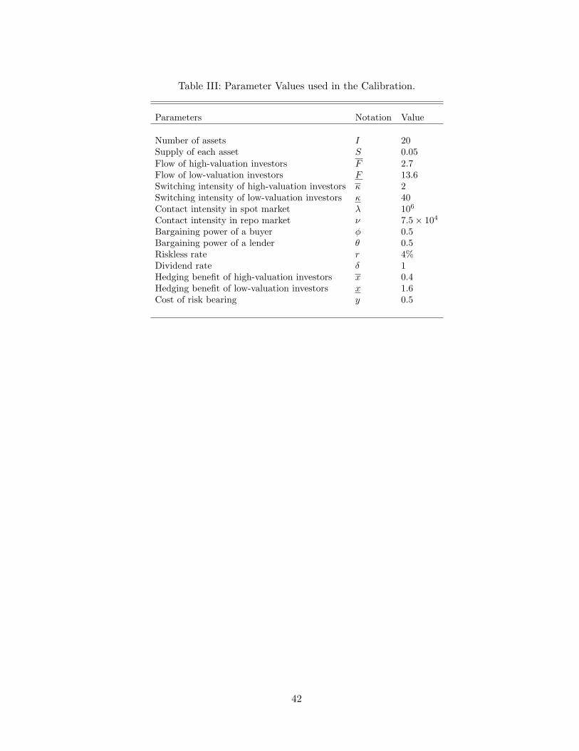
Table III: Parameter Values used in the Calibration.

Parameters Notation Value

Number of assets I 20Supply of each asset S 0.05Flow of high-valuation investors F 2.7Flow of low-valuation investors F 13.6Switching intensity of high-valuation investors κ 2Switching intensity of low-valuation investors κ 40Contact intensity in spot market λ 106

Contact intensity in repo market ν 7.5 × 104

Bargaining power of a buyer φ 0.5Bargaining power of a lender θ 0.5Riskless rate r 4%Dividend rate δ 1Hedging benefit of high-valuation investors x 0.4Hedging benefit of low-valuation investors x 1.6Cost of risk bearing y 0.5

42

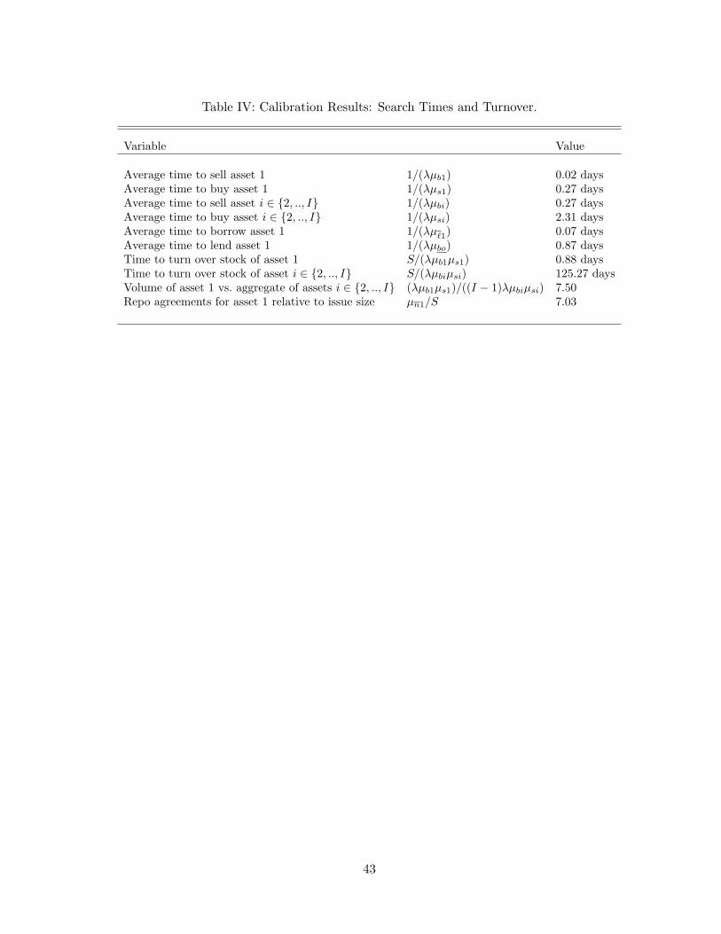
Table IV: Calibration Results: Search Times and Turnover.

Variable Value

Average time to sell asset 1 1/(λμb1) 0.02 daysAverage time to buy asset 1 1/(λμs1) 0.27 daysAverage time to sell asset i ∈ {2, .., I} 1/(λμbi) 0.27 daysAverage time to buy asset i ∈ {2, .., I} 1/(λμsi) 2.31 daysAverage time to borrow asset 1 1/(λμ�1) 0.07 daysAverage time to lend asset 1 1/(λμbo) 0.87 daysTime to turn over stock of asset 1 S/(λμb1μs1) 0.88 daysTime to turn over stock of asset i ∈ {2, .., I} S/(λμbiμsi) 125.27 daysVolume of asset 1 vs. aggregate of assets i ∈ {2, .., I} (λμb1μs1)/((I − 1)λμbiμsi) 7.50Repo agreements for asset 1 relative to issue size μn1/S 7.03

43

Table V: Calibration Results: Prices and Lending Fees.

Variable Value

Expected return of asset 1 δ/p1 5.94%Expected return of asset i ∈ {2, .., I} δ/pi 6.44%Spread δ/pi − δ/p1 50bpsSpecialness w1/p1 35bps

44

Buyer bNon-searcher

niSeller si

Figure 1: Life-cycle. No Short-Sales, Search Spot Market.

45

Buyer b Lender �iRepo

nsi, nni, nbiSeller si

Borrowerbo

Repo

si, ni, bi

Figure 2: Life-cycles. Figure 3 magnifies the two repo boxes.

46

High-valuation High-valuation High-valuation

nsi nni nbi

Seller si Non-searcher

ni

Buyer bi

Figure 3: The states of a lender and a borrower within a repo contract.

47

Notes

1For US evidence, see also Amihud and Mendelson (1991), Krishnamurthy (2002), Goldreich,

Hanke, and Nath (2005), and Strebulaev (2007). For Japan, see Mason (1987), Boudoukh and

Whitelaw (1991), and Boudoukh and Whitelaw (1993).

2On liquidity, Sundaresan (2002) reports that trading volume of on-the-run bonds is about ten

times larger than that of off-the-run, and Fleming (2002) reports that bid-ask spreads of off-the-run

bills are about five times larger than when the bills are on-the-run. Specialness is measured by

comparing a bond’s repo rate, which is the interest rate on a loan collateralized by the bond, to

the general collateral rate, which is the highest quoted repo rate. Duffie (1996) reports an average

specialness of 66bps for on-the-run bonds and 26bps for their off-the-run counterparts.

3In the US, inter-dealer trading is conducted through brokers. Some brokers operate automated

trading systems, structured as electronic limit-order books. Other brokers, however, operate voice-

based systems in which orders are negotiated over the phone. Barclay, Hendershott, and Kotz

(2006) report that automated systems account for about 85% of trading volume for on-the-run

bonds, but the situation is reversed for off-the-run bonds. To explain this phenomenon, they

propose a search-based model.

4The delivery constraint is standard in repo markets: lenders insist on receiving back the same

asset they lent because of considerations of book-keeping, capital-gains taxes, etc. The prevalence

of the delivery constraint is illustrated by the incidence of short-squeezes, whereby short-sellers have

difficulty delivering the asset they borrowed and the asset’s specialness in the repo market increases

dramatically. For a description of short-squeezes see, for example, Dupont and Sack (1999).

5Our multiple-equilibria view seems to fit the Japanese government-bond market: Boudoukh

and Whitelaw (1991) and Boudoukh and Whitelaw (1993) show that the benchmark bond in which

liquidity concentrates can be arbitrary.

6Empirical studies by Cornell and Shapiro (1989), Jordan and Jordan (1997), Buraschi and

Menini (2002), Krishnamurthy (2002), Graveline and McBrady (2007), and Moulton (2004) show

that on-the-run bond prices contain specialness premia consistent with Duffie (1996) and our model.

We return to these studies in Section IV.

7See also Burdett and O’Hara (1987) and Keim and Madhavan (1996) for search-theoretic models

48

of block trading in the upstairs market.

8See also Ellison and Fudenberg (2003) for a general analysis of the coexistence of markets,

and Economides and Siow (1988) for a spatial model of market formation. See also Admati and

Pfleiderer (1988) and Chowdhry and Nanda (1991) for models where trading is concentrated in a

specific time or location because of asymmetric information.

9Hedgers in the Treasury market can be, for example, dealers in corporate bonds or mortgage-

backed securities, who need to hedge the interest-rate risk of their inventories. For a discussion of

hedging in the Treasury market, see Dupont and Sack (1999).

10See Duffie, Garleanu, and Pedersen (2007) for a similar derivation.

11The price differences in these papers compensate buyers for the difficulty in locating an asset.

Suppose, for example, that asset 2 is harder to locate than asset 1. Then, no buyer will search for

asset 2 if its price is greater or equal than asset 1’s. If, however, searching for asset 2 does not

preclude a simultaneous search for asset 1, price differences disappear (as shown in Proposition 2).

12Our analysis assumes that the only delivery method is to buy the asset in the spot market. An

alternative method is through the repo market: short-sellers could borrow the asset from a new

lender and deliver it to the original one. (This method is relevant only when short-sellers wish to

maintain the short position and it is the lender who needs to sell.) One could argue that the ease

of delivering an asset has to do with the repo market, and not with transaction costs in the spot

market. In our model, however, both assets are equally easy to locate in the repo market because

they are in equal supply and thus have the same measure of lenders. Moreover, in practice, while it

might be easier to locate an on- rather than an off-the-run bond in the repo market, such differences

are perceived to be of secondary importance relative to the corresponding differences in the spot

market.

13In this section we take the lender’s strategy as given. We show that the trading strategies of

all agents are optimal in Section III.C, where we establish existence of equilibrium.

14This assumption is for simplicity. An alternative assumption is that the borrower can search

for the asset under a late-delivery penalty, but this would not change the basic intuitions.

In Appendix C we show that because collateral acts as a transfer, its specific value does not

affect any equilibrium variable except the price of the repo contract: high-valuation agents accept

to lend their asset for a lower fee if they can seize more collateral. To downplay this effect, we

49

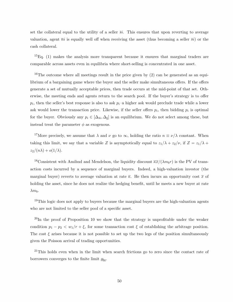
set the collateral equal to the utility of a seller si. This ensures that upon reverting to average

valuation, agent ni is equally well off when receiving the asset (thus becoming a seller si) or the

cash collateral.

15Eq. (1) makes the analysis more transparent because it ensures that marginal traders are

comparable across assets even in equilibria where short-selling is concentrated in one asset.

16The outcome where all meetings result in the price given by (2) can be generated as an equi-

librium of a bargaining game where the buyer and the seller make simultaneous offers. If the offers

generate a set of mutually acceptable prices, then trade occurs at the mid-point of that set. Oth-

erwise, the meeting ends and agents return to the search pool. If the buyer’s strategy is to offer

pi, then the seller’s best response is also to ask pi–a higher ask would preclude trade while a lower

ask would lower the transaction price. Likewise, if the seller offers pi, then bidding pi is optimal

for the buyer. Obviously any pi ∈ [Δsi, Δb] is an equilibrium. We do not select among these, but

instead treat the parameter φ as exogenous.

17More precisely, we assume that λ and ν go to ∞, holding the ratio n ≡ ν/λ constant. When

taking this limit, we say that a variable Z is asymptotically equal to z1/λ + z2/ν, if Z = z1/λ +

z2/(nλ) + o(1/λ).

18Consistent with Amihud and Mendelson, the liquidity discount κx/(λmbr) is the PV of trans-

action costs incurred by a sequence of marginal buyers. Indeed, a high-valuation investor (the

marginal buyer) reverts to average valuation at rate κ. He then incurs an opportunity cost x of

holding the asset, since he does not realize the hedging benefit, until he meets a new buyer at rate

λmb.

19This logic does not apply to buyers because the marginal buyers are the high-valuation agents

who are not limited to the seller pool of a specific asset.

20In the proof of Proposition 10 we show that the strategy is unprofitable under the weaker

condition p1 − p2 < w1/r + ξ, for some transaction cost ξ of establishing the arbitrage position.

The cost ξ arises because it is not possible to set up the two legs of the position simultaneously

given the Poisson arrival of trading opportunities.

21This holds even when in the limit when search frictions go to zero since the contact rate of

borrowers converges to the finite limit gbo.

50

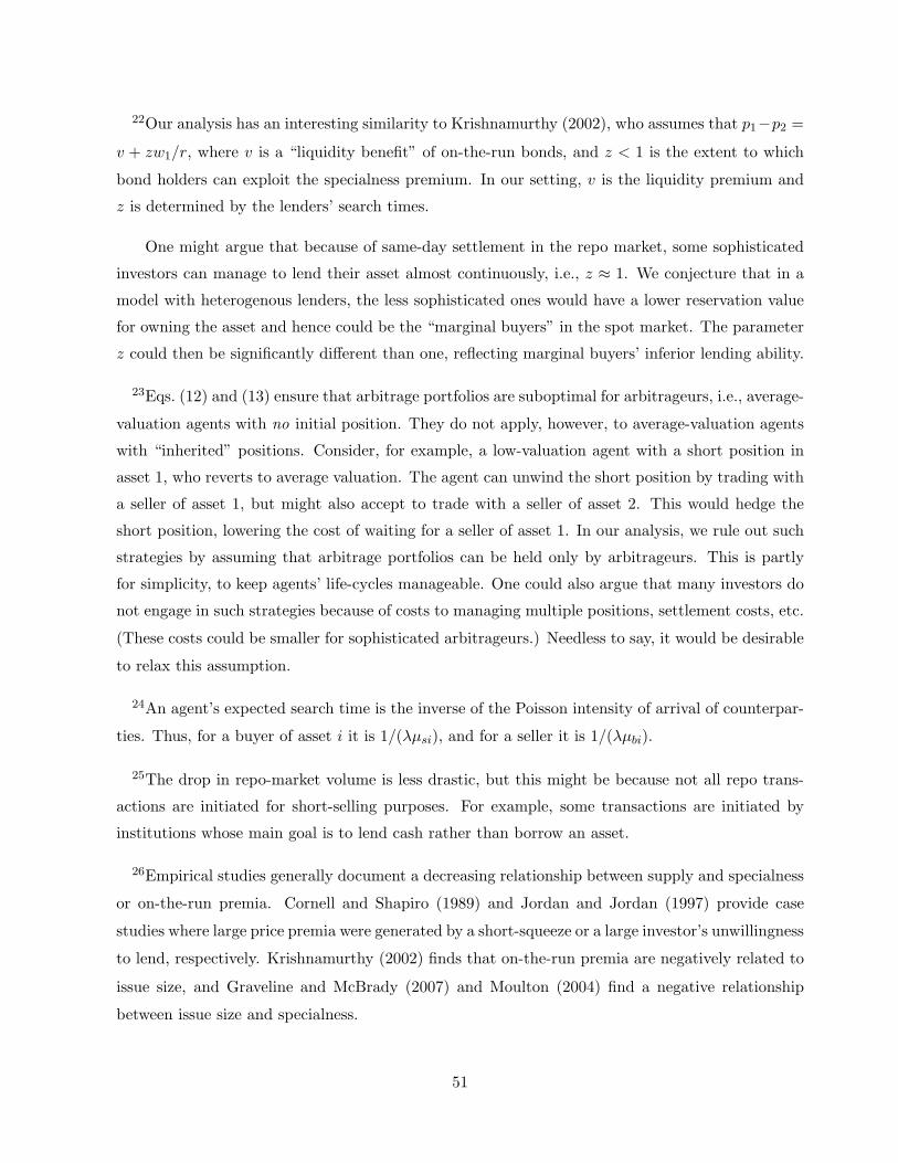
22Our analysis has an interesting similarity to Krishnamurthy (2002), who assumes that p1−p2 =

v + zw1/r, where v is a “liquidity benefit” of on-the-run bonds, and z < 1 is the extent to which

bond holders can exploit the specialness premium. In our setting, v is the liquidity premium and

z is determined by the lenders’ search times.

One might argue that because of same-day settlement in the repo market, some sophisticated

investors can manage to lend their asset almost continuously, i.e., z ≈ 1. We conjecture that in a

model with heterogenous lenders, the less sophisticated ones would have a lower reservation value

for owning the asset and hence could be the “marginal buyers” in the spot market. The parameter

z could then be significantly different than one, reflecting marginal buyers’ inferior lending ability.

23Eqs. (12) and (13) ensure that arbitrage portfolios are suboptimal for arbitrageurs, i.e., average-

valuation agents with no initial position. They do not apply, however, to average-valuation agents

with “inherited” positions. Consider, for example, a low-valuation agent with a short position in

asset 1, who reverts to average valuation. The agent can unwind the short position by trading with

a seller of asset 1, but might also accept to trade with a seller of asset 2. This would hedge the

short position, lowering the cost of waiting for a seller of asset 1. In our analysis, we rule out such

strategies by assuming that arbitrage portfolios can be held only by arbitrageurs. This is partly

for simplicity, to keep agents’ life-cycles manageable. One could also argue that many investors do

not engage in such strategies because of costs to managing multiple positions, settlement costs, etc.

(These costs could be smaller for sophisticated arbitrageurs.) Needless to say, it would be desirable

to relax this assumption.

24An agent’s expected search time is the inverse of the Poisson intensity of arrival of counterpar-

ties. Thus, for a buyer of asset i it is 1/(λμsi), and for a seller it is 1/(λμbi).

25The drop in repo-market volume is less drastic, but this might be because not all repo trans-

actions are initiated for short-selling purposes. For example, some transactions are initiated by

institutions whose main goal is to lend cash rather than borrow an asset.

26Empirical studies generally document a decreasing relationship between supply and specialness

or on-the-run premia. Cornell and Shapiro (1989) and Jordan and Jordan (1997) provide case

studies where large price premia were generated by a short-squeeze or a large investor’s unwillingness

to lend, respectively. Krishnamurthy (2002) finds that on-the-run premia are negatively related to

issue size, and Graveline and McBrady (2007) and Moulton (2004) find a negative relationship

between issue size and specialness.

51

27For example, on February 2, 2005, primary dealers reported asset loans of about $2 trillion

(New York Fed website, www.ny.frb.org/markets/gsds/search.cfm). Since the Treasury market

is worth about $4 trillion, of which 5% are on-the-run bonds, the amount of repo agreements exceeds

the market value of on-the-run bonds by about 2/(4 × 5%) = 10. We select a number below ten

to account for repo activity in off-the-run bonds. A higher number would strengthen our results

because the lending fee would increase.

28Suppose, for example, that the average Treasury security turns over in twelve trading days.

Since on-the-run bonds account for about 5% of market capitalization and 10/11 of trading volume,

they turn over in 5% × 12/(10/11) = 0.66 days, while off-the-run bonds turn over in 95% ×12/(1/11) = 125.4 days.

29The six-day expected horizon of short-sellers is approximately equal to the turnover time of

the asset supply that they generate (F/κ). This supply is about seven times the issue size S, and

turns over seven times more slowly.

30US Treasury securities are traded round the clock in New York, London, and Tokyo. However,

Fleming (1997) reports that 94% of the trading takes place in New York from 7:30am to 5:30pm.

31The search times in Table IV appear especially short if we consider the implied transaction

costs. For example, the cost incurred by a high-valuation buyer is not to receive the hedging benefit

x while searching. With a search time of 0.12 days, i.e., 0.12/250 of a year, the search cost is a

fraction x × (0.12/250)/(1/6.44%) = 1.2 × 10−5 of the price, i.e., 0.12 cents per $100 transaction

value. Likewise, the search cost of a low-valuation agent seeking to borrow asset 1 in the repo market

is not to receive the hedging benefit x. This cost is a fraction x×(0.07/250)/(1/6.44%) = 2.9×10−5

of the price, i.e., 0.29 cents per $100 transaction value. Such costs are smaller than the average

bid-ask spread in the Treasury market, which is 1.1 cent (Dupont and Sack (1999)).

32Matching the risk premium of long-term bonds is only one condition, while there are two

parameters (x, y). The second degree of freedom in these parameters appears to have a small effect

on the calibration results.

33Some studies find smaller effects. For example, Fleming (2003) reports that on-the-run bonds

yield 5.6bps below off-the-run bonds, and Goldreich, Hanke, and Nath (2005) report 1.5bps. These

papers, however, focus on bonds with a long time to maturity, for which the three-month conve-

nience yield of being on-the-run has only a small effect on the yield to maturity. Warga (1992)

52

compares the returns of on- and off-the-run bond portfolios rather than their yields to maturity.

This isolates the on-the-run convenience yield in exactly the same way as in this paper. Amihud

and Mendelson (1991) compare yields to maturity, but can isolate the convenience yield because

they focus on securities with very short times to maturity. They find that Treasury bills maturing

in less than six months yield 38bps below comparable Treasury notes.

34The expected return spread δ/pi − δ/p1 in Table V is greater than the lending fee w1/p1. This

suggests an arbitrage strategy of shorting $1 of asset 1, paying the lending fee, and buying $1 of asset

2. The payoff of this strategy is risky, however, because the assets are held in different quantities.

Adjusting for risk amounts to calculating the marginal utility flow (δ − y)/pi − (δ − y)/p1 −w1/p1

that an arbitrageur would derive, which turns out to be negative.

53