A search for factors causing training costs to rise by

Calhoun: The NPS Institutional Archive

Theses and Dissertations Thesis Collection

1986-09

A search for factors causing training costs to rise by

examining the U.S. Navy's AT, AW, and AX ratings

during their first enlistment period

Aiu, Eugene K.

Monterey, California: U.S. Naval Postgraduate School

http://hdl.handle.net/10945/22088

[OOL

NAVAL POSTGRADUATE SCHOOL

Monterey, California

THESISA SEARCH FOR FACTORS CAUSING TRAINING COSTS TO RISE

BY EXAMINING THE U.S. NAVY'S AT, AW, AND AX

RATINGS DURING THEIR FIRST ENLISTMENT PERIOD

by

Eugene Kapua Aiu

September 1986

Thesis Advisor: Dan C. Boger

Approved for public release; distribution is unlimited

T230025

security Classification Of Thi$ page

REPORT DOCUMENTATION PAGE

la REPORT SECURITY CLASSIFICATION

UNCLASSIFIEDlb. RESTRICTIVE MARKINGS

2a SECURITY CLASSIFICATION AUTHORITY

2b DECLASSIFICATION /DOWNGRADING SCHEDULE

3 DISTRIBUTION /AVAILABILITY OF REPORT

Approved for public release; distributionis unlimited.

4 PERFORMING ORGANIZATION REPORT NUMBER(S)

6a. NAME OF PERFORMING ORGANIZATION

Naval Postgraduate School

6b OFFICE SYMBOL(If applicable)

Code 55

5 MONITORING ORGANIZATION REPORT NUMBER(S)

7a NAME OF MONITORING ORGANIZATION

Naval Postgraduate School

6c ADDRESS (City. State, and ZIP Code)

Monterey, California 93943-5000

7b. ADDRESS {City. State, and ZIP Code)

Monterey, California 93943-5000

8a NAME OF FUNDING / SPONSORINGORGANIZATION

8b OFFICE SYMBOL(If applicable)

9 PROCUREMENT INSTRUMENT IDENTIFICATION NUMBER

8c ADDRESS (City. State, and ZIP Code) 10 SOURCE OF FUNDING NUMBERS

PROGRAMELEMENT NO

PROJECTNO

TAS<NO

WORK UNITACCESSION NO

n TITLE (Include Security Classification)

A SEARCH FOR FACTORS CAUSING TRAINING COSTS TO RISE BY EXAMINING THE U.S. NAVY'S AT, AW,

AND AX RATINGS DURING THEIR FIRST ENLISTMENT PERIOD

12 PERSONAL AUTHOR(S)Aiu, Eugene K.

'3a TYPE OF REPORTMaster ' s Thesis

13b TIME COVEREDFROM TO

14 DATE OF REPORT (Year, Month, Day)

1986 September15 PAGE COUNT

120

6 SUPPLEMENTARY NOTATION

COSATI CODES

;Eld GROUP SUB-GROUP

18 SUBJECT TERMS (Continue on reverse if necessary and identify by block number)

Manpower Study, AT, AW, AX, Length of Basic Training,

Amount of Specialized Training, Attrition

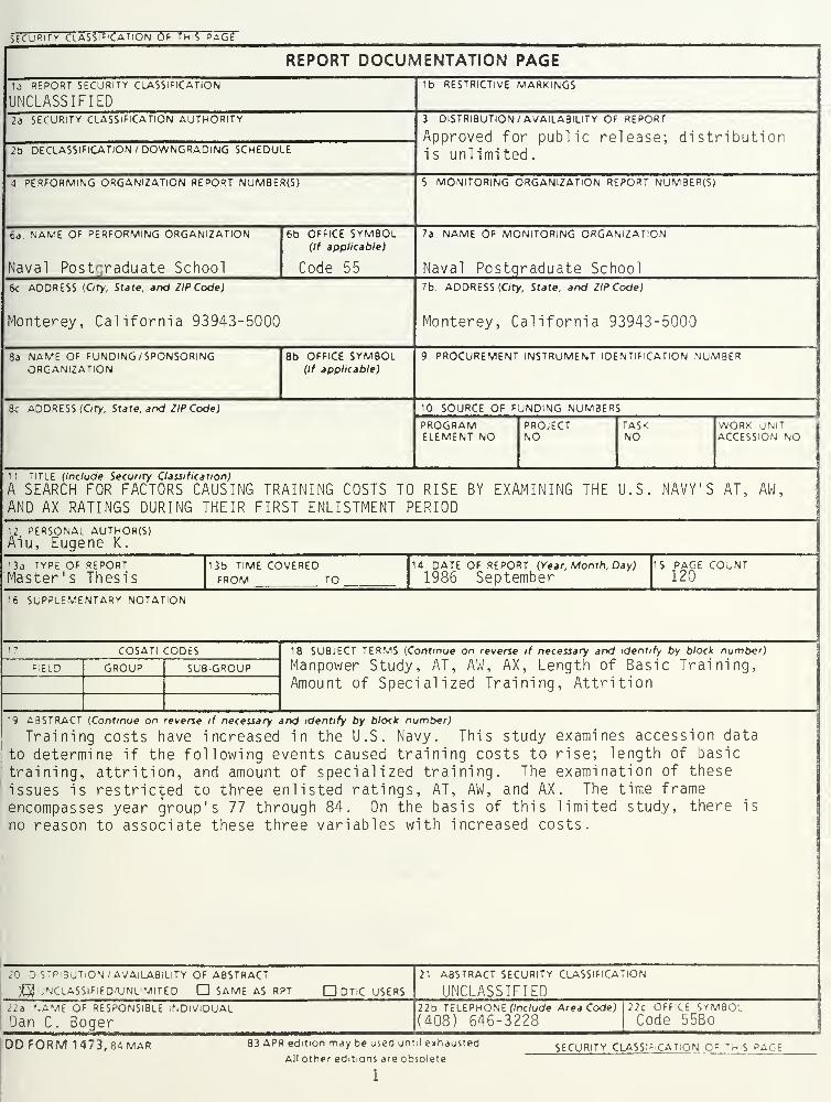
'9 ABSTRACT (Continue on reverse if necessary and identify by block number)

Training costs have increased in the U.S. Navy. This study examines accession data

to determine if the following events caused training costs to rise; length of basic

training, attrition, and amount of specialized training. The examination of these

issues is restricted to three enlisted ratings, AT, AW, and AX. The time frame

encompasses year group's 77 through 84. On the basis of this limited study, there is

no reason to associate these three variables with increased costs.

20 D S~P'3UTiON/ AVAILABILITY OF ABSTRACT

£)? ,'NCLASSlFiED/UNL'MITED SAME AS RPT DdTiC USERS

21 ABSTRACT SECURITY CLASSIFICATION

UNCLASSIFIED22a NAME OF RESPONSIBLE INDIVIDUAL

Dan C. Soger22b TELEPHONE (Include Area Code)

(408) 646-322822c OFFICE SYMBOLCode 55Bo

DDFORM 1473, 84 mar 83 APR edition may be used until exhausted

All other edition? are obsoleteSECURITY CLASSIFICATION OF this PAGE

Approved for public release; distribution is unlimited.

A search for factors causing training costs to rise

by examining the U.S. Navy's AT, AW, and AX ratings

during their first enlistment period.

by

Eugene Kapua AiuLieutenant, United States NavyB.S., Marquette University, 1979

Submitted in partial fulfillment of the

requirements for the degree of

MASTER OF SCIENCE IN OPERATIONS RESEARCH

from the

NAVAL POSTGRADUATE SCHOOLSeptember 1986

ABSTRACT

Training costs have increased in the U.S. Navy. This study examines accession

data to determine if the following events caused training costs to rise; length of basic

training, attrition, and amount of specialized training. The examination of these issues

is restricted to three enlisted ratings, AT, AW, and AX. The time frame encompasses

year group's 77 through 84. On the basis of this limited study, there is no reason to

associate these three variables with increased costs.

TABLE OF CONTENTS

I. INTRODUCTION 9

A. PROBLEM STATEMENT 9

B. OBJECTIVES 10

II. HISTORY AND BACKGROUND 11

A. DATA BASE DESCRIPTION 11

B. EXPECTED TRAINING PATH 12

C. LIMITATIONS 13

D. SCOPE 13

1

.

Length of Basic Training 13

2. Attrition 16

3. Amount of specialized training 16

III. METHODOLOGY AND ANALYSIS 19

A. BASIC TRAINING 19

1. Time to get rated: Is there a trend? 19

2. Has the time to get rated increased or decreased through1983? 21

B. ATTRITION 28

1. Percent Losses: Is it rising? 28

2. Attrition rates: Is it rising? 41

C. SPECIALIZED TRAINING 57

1. Average number of NEC's per individual: Has it

increased? 61

2. Average number of NEC's per year group: Has it

increased? 62

IV. MAIN RESULTS AND CONCLUSIONS 79

A. SUMMARY 79

B. RECOMMENDATIONS 83

APPENDIX A: MODEL ASSUMPTIONS 84

1. REGRESSION 85

a. The relationship is linear 85

b. The errors are independent and have constant variance 85

c. The error terms are normal 86

2. ANALYSIS OF VARIANCE 86

a. The populations are normally distributed 86

b. The population variances are equal 87

c. The error terms are independent 89

d. The error terms have constant variance 89

e. The error terms are normally distributed 90

APPENDIX B: DATA BASE 104

APPENDIX C: PROGRAM LISTING 108

APPENDIX D: DATA VECTORS Ill

LIST OF REFERENCES 117

BIBLIOGRAPHY 118

INITIAL DISTRIBUTION LIST 119

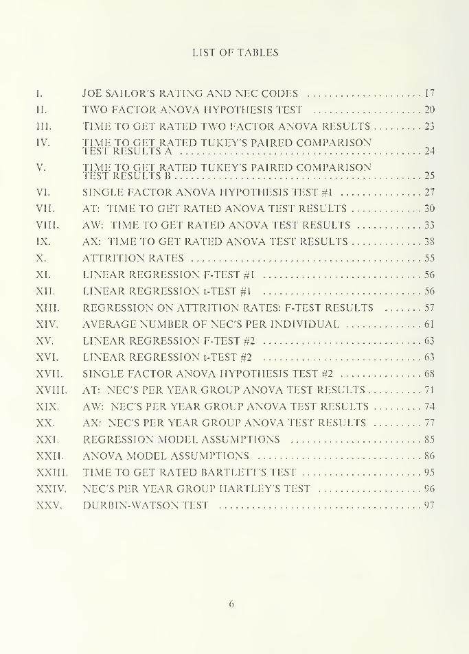
LIST OF TABLES

I. JOE SAILOR'S RATING AND NEC CODES 17

II. TWO FACTOR ANOVA HYPOTHESIS TEST 20

III. TIME TO GET RATED TWO FACTOR ANOVA RESULTS 23

IV. TIME TO GET RATED TUKEY'S PAIRED COMPARISONTEST RESULTS A 24

V. TIME TO GET RATED TUKEY'S PAIRED COMPARISONTEST RESULTS B 25

VI. SINGLE FACTOR ANOVA HYPOTHESIS TEST #1 27

VII. AT: TIME TO GET RATED ANOVA TEST RESULTS 30

VIII. AW: TIME TO GET RATED ANOVA TEST RESULTS 33

IX. AX: TIME TO GET RATED ANOVA TEST RESULTS 38

X. ATTRITION RATES 55

XL LINEAR REGRESSION F-TEST #1 56

XII. LINEAR REGRESSION t-TEST #1 56

XIII. REGRESSION ON ATTRITION RATES: F-TEST RESULTS 57

XIV. AVERAGE NUMBER OF NEC'S PER INDIVIDUAL 61

XV. LINEAR REGRESSION F-TEST #2 63

XVI. LINEAR REGRESSION t-TEST #2 63

XVII. SINGLE FACTOR ANOVA HYPOTHESIS TEST #2 68

XVIII. AT: NEC'S PER YEAR GROUP ANOVA TEST RESULTS 71

XIX. AW: NEC'S PER YEAR GROUP ANOVA TEST RESULTS 74

XX. AX: NEC'S PER YEAR GROUP ANOVA TEST RESULTS 77

XXI. REGRESSION MODEL ASSUMPTIONS 85

XXII. ANOVA MODEL ASSUMPTIONS 86

XXIII. TIME TO GET RATED BARTLETT'S TEST 95

XXIV. NEC'S PER YEAR GROUP HARTLEY'S TEST 96

XXV. DURBIN-WATSON TEST 97

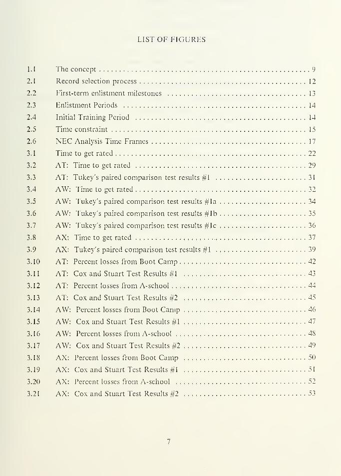
LIST OF FIGURES

1.1 The concept 9

2.1 Record selection process 12

2.2 First-term enlistment milestones 13

2.3 Enlistment Periods 14

2.4 Initial Training Period 14

2.5 Time constraint 15

2.6 NEC Analysis Time Frames 17

3.

1

Time to get rated 22

3.2 AT: Time to get rated 29

3.3 AT: Tukey's paired comparison test results #1 31

3.4 AW: Time to get rated 32

3.5 AW: Tukey's paired comparison test results #la 34

3.6 AW: Tukey's paired comparison test results #lb 35

3.7 AW: Tukey's paired comparison test results #lc 36

3.8 AX: Time to get rated 37

3.9 AX: Tukey's paired comparison test results #1 39

3.10 AT: Percent losses from Boot Camp 42

3.11 AT: Cox and Stuart Test Results #1 43

3.12 AT: Percent losses from A-school 44

3.13 AT: Cox and Stuart Test Results #2 45

3.14 AW: Percent losses from Boot Camp 46

3.15 AW: Cox and Stuart Test Results #1 47

3.16 AW: Percent losses from A-school 48

3.17 AW: Cox and Stuart Test Results #2 49

3.18 AX: Percent losses from Boot Camp 50

3.19 AX: Cox and Stuart Test Results #1 51

3.20 AX: Percent losses from A-school 52

3.21 AX: Cox and Stuart Test Results #2 53

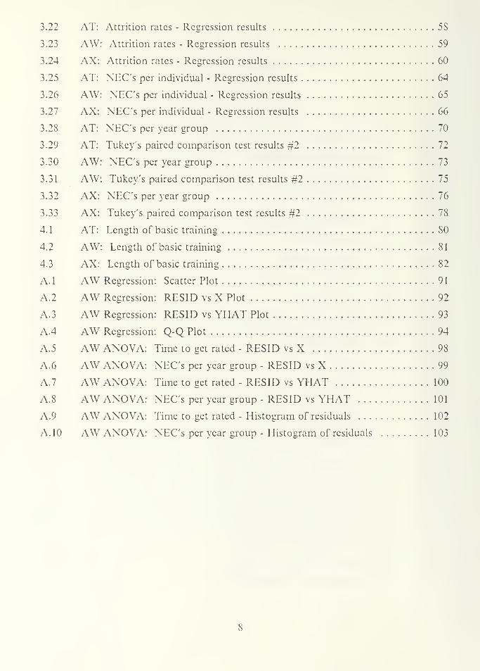
3.22

3.23

3.24

3.25

3.26

3.27

3.28

3.29

3.30

3.31

3.32

3.33

4.1

4.2

4.3

A.l

A.

2

A. 3

A.4

A.5

A.6

A.7

A. 8

A.9

A. 10

AT: Attrition rates - Regression results 58

AW: Attrition rates - Regression results 59

AX: Attrition rates - Regression results 60

AT: NEC's per individual - Regression results 64

AW: NEC's per individual - Regression results 65

AX: NEC's per individual - Regression results 66

AT: NEC's per year group 70

AT: Tukey's paired comparison test results #2 72

AW: NEC's per year group 73

AW: Tukey's paired comparison test results #2 75

AX: NEC's per year group 76

AX: Tukey's paired comparison test results #2 78

AT: Length of basic training SO

AW: Length of basic training 81

AX: Length of basic training 82

AW Regression: Scatter Plot 91

AW Regression: RESID vs X Plot 92

AW Regression: RESID vs YHAT Plot 93

AW Regression: Q-Q Plot 94

AW ANOVAAW ANOVAAW ANOVAAW ANOVAAW ANOVAAW ANOVA

Time to get rated - RESID vs X 98

NEC's per year group - RESID vs X 99

Time to get rated - RESID vs YHAT 100

NEC's per year group - RESID vs YHAT 101

Time to get rated - Histogram of residuals 102

NEC's per year group - Histogram of residuals 103

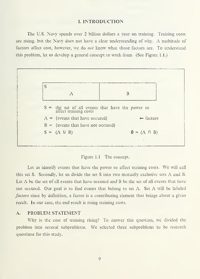
I. INTRODUCTION

The U.S. Navy spends over 2 billion dollars a year on training. Training costs

are rising, but the Navy does not have a clear understanding of why. A multitude of

factors affect cost, however, we do not know what those factors are. To understand

this problem, let us develop a general concept to work from. (See Figure 1.1.)

S

A B

S = the set of all events that have the power toaffect training costs

A = {events that have occured} «- factors

B = {events that have not occured}

S = (A U B) = (A n B)

Figure 1.1 The concept.

Let us identify events that have the power to affect training costs. We will call

this set S. Secondly, let us divide the set S into two mutually exclusive sets A and B.

Let A be the set of all events that have occured and B be the set of all events that have

not occured. Our goal is to find events that belong to set A. Set A will be labeled

factors since by definition, a factor is a contributing clement that brings about a given

result. In our case, the end result is rising training costs.

A. PROBLEM STATEMENT

Why is the cost of training rising? To answer this question, we divided the

problem into several subproblems. We selected three subproblems to be research

questions for this study.

• Has the length of basic training increased*.

• Has attrition increased.

• Has the amount of specialized training increased!

Our goal is to identify events that affect training costs. Imbedded within our

problem statment are three events. These events are:

A. The length of basic training has increased.

B. Attrition has increased.

C. The amount of specialized training has increased.

Can we classify any of these events as factors! Or stated differently, "Have any of

these events occured?" If event A, B, or C occured, then at least one reason will exist

to explain the rise in training cost.

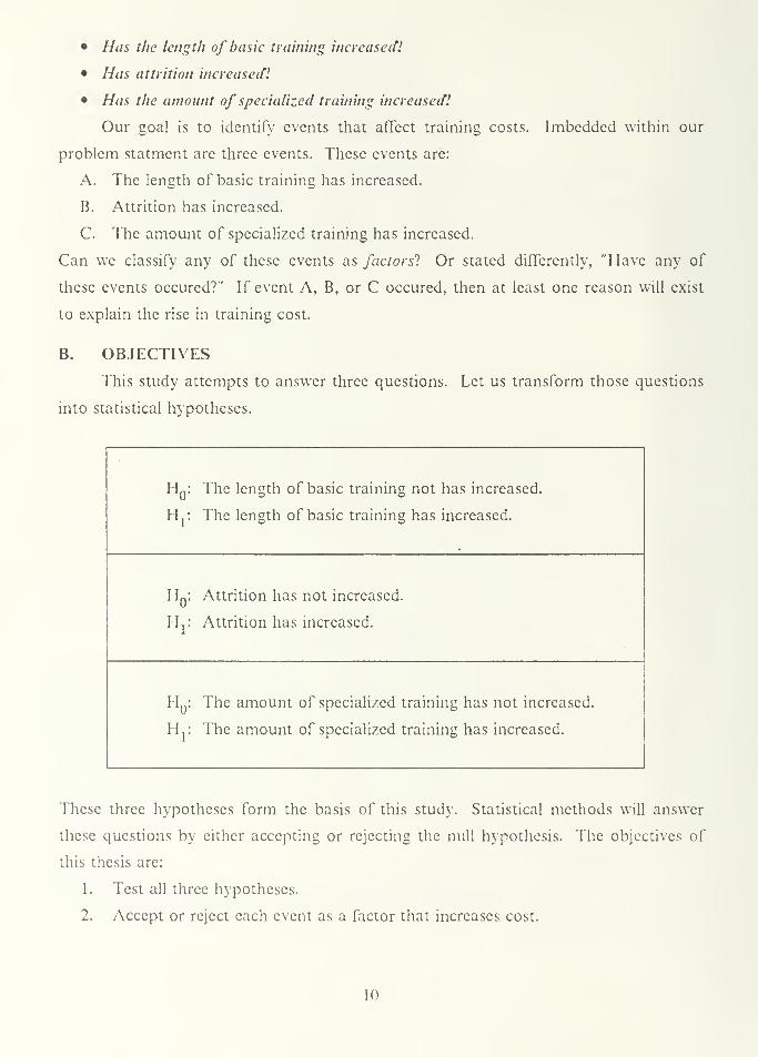
B. OBJECTIVES

This study attempts to answer three questions. Let us transform those questions

into statistical hypotheses.

HQ

: The length of basic training not has increased.

H,: The length of basic training has increased.

FL: Attrition has not increased.

H,: Attrition has increased.

H : The amount of specialized training has not increased.

Hji The amount of specialized training has increased.

These three hypotheses form the basis of this study. Statistical methods will answer

these questions by either accepting or rejecting the null hypothesis. The objectives of

this thesis are:

1. Test all three hypotheses.

2. Accept or reject each event as a factor that increases cost.

10

II. HISTORY AND BACKGROUND

The Chief of Naval Operartions (CNO) expected training costs to fall when

retention increased in the early 19S0's. However, a decrease did not occur. The Center

for Naval Analyses (CNA) was tasked to examine the relationships between training

costs and retention. CNA formulated some general reasons why training costs might

change. They set out to confirm those reasons by using information stored in their

historical data files. From those data files, they provided a small data base for this

study.

A. DATA BASE DESCRIPTION

The Navy has 101 enlisted rating codes. CNA's data set contains information on

every enlisted rating. The data base used for this study contains information on only

three enlisted ratings. These ratings are:

AT = Aviation Technician

AW = Aviation Anti-Submarine Warfare Operator

AX = Aviation Anti-Submarine Warfare Technician

We selected these ratings for the following reasons. This author, in conjuction with

CNA, expressed an interest to examine the aviation community. Next, we decided to

observe two closely related technical ratings from a squadron's maintenance

department, so we selected the AT's and AX's. Lastly, we wanted to observe a rating

from the squadron's operations department, so we selected the AW's.

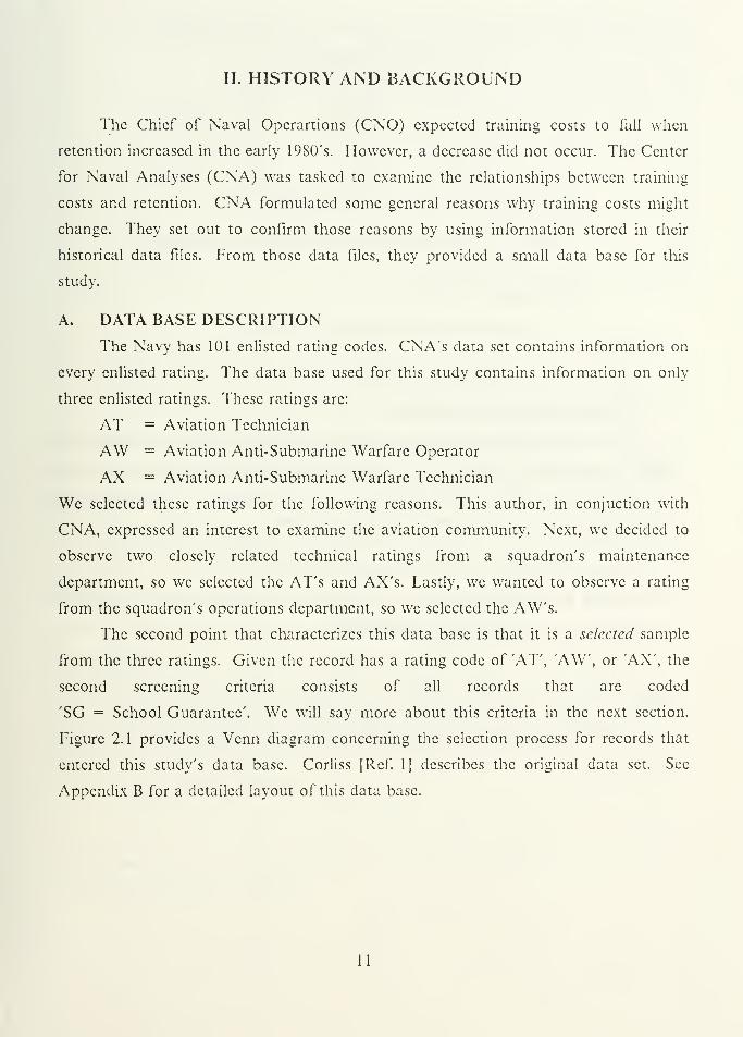
The second point that characterizes this data base is that it is a selected sample

from the three ratings. Given the record has a rating code of 'AT', AW', or 'AX', the

second screening criteria consists of all records that are coded

'SG = School Guarantee'. We will say more about this criteria in the next section.

Figure 2.1 provides a Venn diagram concerning the selection process for records that

entered this study's data base. Corliss [Ref. 1] describes the original data set. See

Appendix B for a detailed layout of this data base.

11

CNA's Data Set

CDA = (AT U AW U AX)

Data Base = (A n B)

B == (SG)

Figure 2.1 Record selection process.

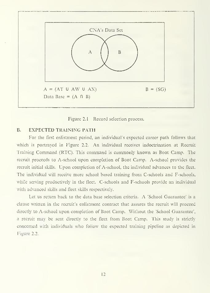
B. EXPECTED TRAINING PATH

For the first enlistment period, an individual's expected career path follows that

which is portrayed in Figure 2.2. An individual receives indoctrination at Recruit

Training Command (RTC). This command is commonly known as Boot Camp. The

recruit proceeds to A-school upon completion of Boot Camp. A-school provides the

recruit initial skills. Upon completion of A-school, the individual advances to the fleet.

The individual will receive more school based training from C-schools and F-schools,

while serving productively in the fleet. C-schools and F-schools provide an individual

with advanced skills and fleet skills respectively.

Let us return back to the data base selection criteria. A 'School Guarantee' is a

clause written in the recruit's enlistment contract that assures the recruit will proceed

directly to A-school upon completion of Boot Camp. Without the 'School Guarantee',

a recruit may be sent directly to the fleet from Boot Camp. This study is strictly

concerned with individuals who follow the expected training pipeline as depicted in

Figure 2.2.

12

EXPECTED CAREER PATH

Boot Camp A-School * Fleet *

i

i

Training Period Productive Period

* While serving in the fleet, a person will receive training fromC-Schools and E-Schools.

Figure 2.2 First-term enlistment milestones.

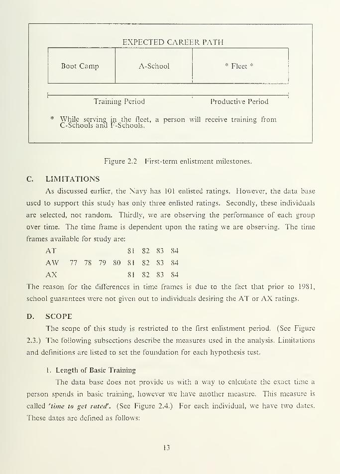
C. LIMITATIONS

As discussed earlier, the Navy has 101 enlisted ratings. However, the data base

used to support this study has only three enlisted ratings. Secondly, these individuals

are selected, not random. Thirdly, we are observing the performance oC each group

over time. The time frame is dependent upon the rating we are observing. The time

frames available for study are:

AT 81 82 83 84

AW 77 78 79 80 81 82 83 84

AX 81 82 S3 84

The reason for the differences in time frames is due to the fact that prior to 1981,

school guarantees were not given out to individuals desiring the AT or AX ratings.

D. SCOPE

The scope of this study is restricted to the first enlistment period. (See Figure

2.3.) The following subsections describe the measures used in the analysis. Limitations

and definitions are listed to set the foundation for each hypothesis test.

1. Length of Basic Training

The data base does not provide us with a way to calculate the exact time a

person spends in basic training, however we have another measure. This measure is

called 'time to get rated'. (See Figure 2.4.) For each individual, we have two dates.

These dates are defined as follows:

13

ENLISTMENT PERIODS

1st 2nd

3rd

1 1 1

1

PEBD EAOS EAOS- EAOS-

PEBD = PAY ENTRY BASE DATE

EAOS = END OF ACTIVE OBLIGATED SERVICE

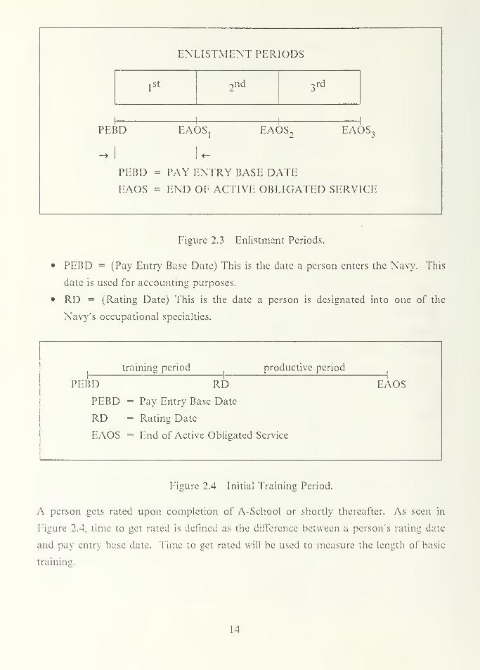
Figure 2.3 Enlistment Periods.

• PEBD = (Pay Entry Base Date) This is the date a person enters the Navy. This

date is used for accounting purposes.

• RD = (Rating Date) This is the date a person is designated into one of the

Navy's occupational specialties.

training period productive period

PEBD RD

PEBD = Pay Entry Base Date

RD = Rating Date

EAOS = End of Active Obligated Service

EAOS

Figure 2.4 Initial Training Period.

A person gets rated upon completion of A-School or shortly thereafter. As seen in

Figure 2.4, time to get rated is defined as the difference between a person's rating date

and pay entry base date. Time to get rated will be used to measure the length of basic

training.

14

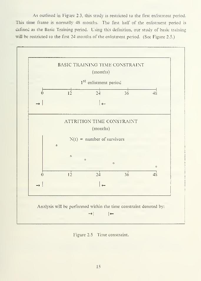
As outlined in Figure 2.3, this study is restricted to the first enlistment period.

This time frame is normally 48 months. The first half of the enlistment period is

defined as the Basic Training period. Using this definition, our study of basic training

will be restricted to the first 24 months of the enlistment period. (See Figure 2.5.)

BASIC TRAINING TIME CONSTRAINT

(months)

c

1st

enlistment period

i i i

1

1 ! 1

> 12 24 36 4S

—

»

1«-

ATTRITION TIME CONSTRAINT

(months)

N(t) = number of survivors

*J.

*

(

#

) 12 24 36 48

—1«—

Analysis will be performed within the time constraint denoted by:

Figure 2.5 Time constraint.

15

2. Attrition

Percent losses and attrition rates are the measures used to compare year

groups. Given a year group, percent loss is defined as the number of individuals that

leave the Navy divided by the number of individuals that enlisted in the Navy.

Attrition rate is defined as the number of individuals that leave the Navy per month.

We restrict our analysis to the first 24 months per year group. Our goal is to measure

attrition in the training environment and not in the operational environment. (See

Figure 2.5.)

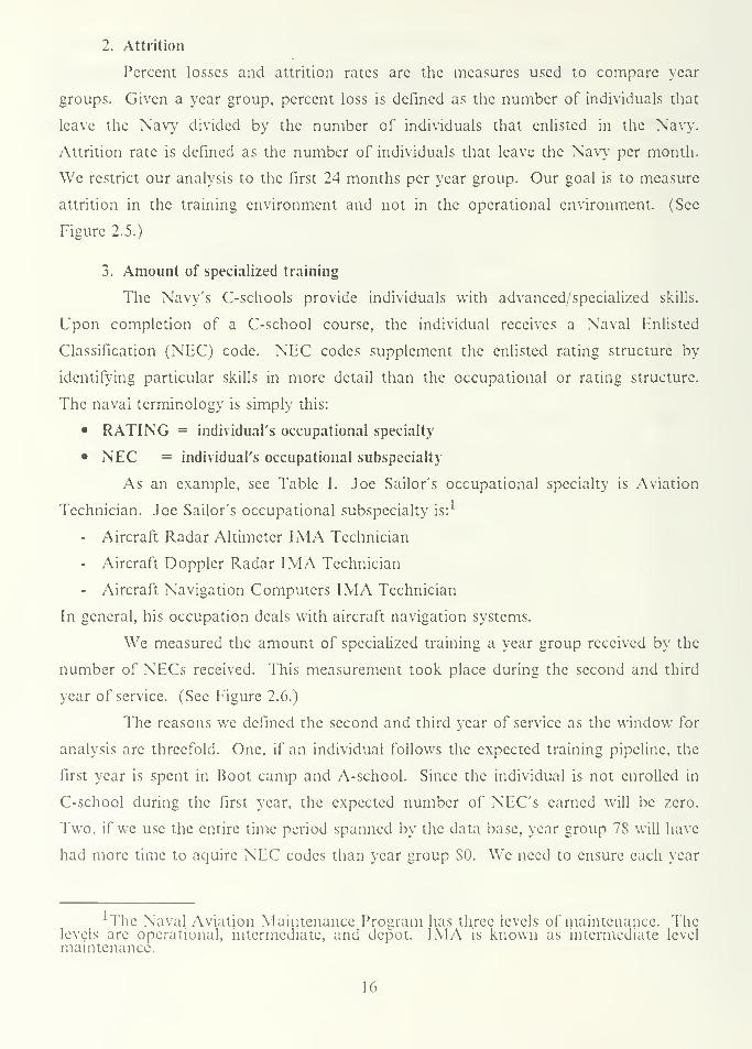
3. Amount of specialized training

The Navy's C-schools provide individuals with advanced/specialized skills.

Upon completion of a C-school course, the individual receives a Naval Enlisted

Classification (NEC) code. NEC codes supplement the enlisted rating structure by

identifying particular skills in more detail than the occupational or rating structure.

The navai terminology is simply this:

• RATING = individual's occupational specialty

• NEC = individual's occupational subspecialty

As an example, see Table I. Joe Sailor's occupational specialty is Aviation

Technician. Joe Sailor's occupational subspecialty is:1

- Aircraft Radar Altimeter IMA Technician

- Aircraft Doppler Radar IMA Technician

- Aircraft Navigation Computers IMA Technician

In general, his occupation deals with aircraft navigation systems.

We measured the amount of specialized training a year group received by the

number of NECs received. This measurement took place during the second and third

year of service. (See Figure 2.6.)

The reasons we defined the second and third year of service as the window for

analysis are threefold. One, if an individual follows the expected training pipeline, the

first year is spent in Boot camp and A-school. Since the individual is not enrolled in

C-school during the first year, the expected number of NEC's earned will be zero.

Two, if we use the entire time period spanned by the data base, year group 7S will have

had more time to aquire NEC codes than year group SO. We need to ensure each year

The Naval Aviation Maintenance Program has three levels of maintenance. Thelevels are operational, intermediate, and depot. IMA is known as intermediate levelmaintenance.

16

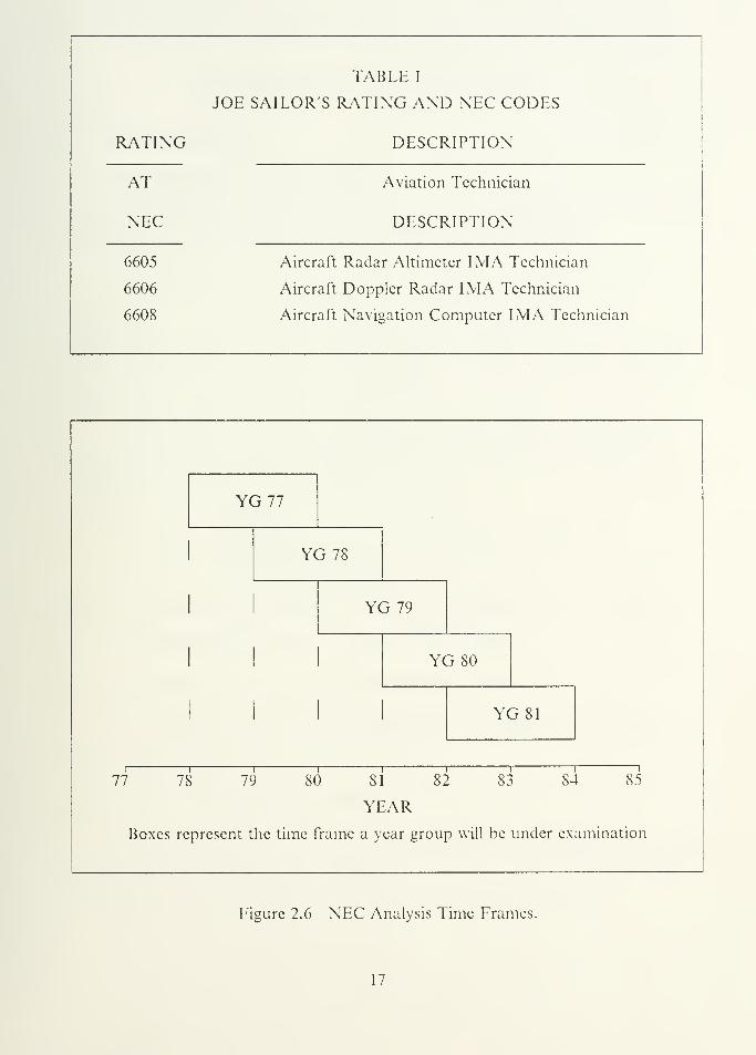
TABLE I

JOE SAILOR'S RATING AND NEC CODES

RATING DESCRIPTION

AT Aviation Technician

NEC DESCRIPTION

6605 Aircraft Radar Altimeter IMA Technician

6606 Aircraft Doppler Radar IMA Technician

6608 Aircraft Navigation Computer IMA Technician

YG77

YG 78

YG 79

11

YG 80

1 1 1 YG 81

11~ 78 79 80 SI 82 83 S4 ~~85

YEAR

Boxes represent the time frame a year group will be under examination

Figure 2.6 NEC Analysis Time Frames.

17

group has exactly the same time length and the same time period in their respective

careers to accumulate NEC codes. Three, we stated earlier that our analysis will be

restricted to the first enlistment period.

18

III. METHODOLOGY AND ANALYSIS

A. BASIC TRAINING

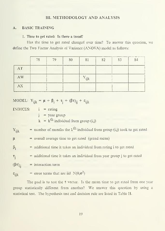
1. Time to get rated: Is there a trend?

Has the time to get rated changed over time? To answer this question, we

define the Two Factor Analysis of Variance (ANOVA) model as follows:

78 79 80 81 82 83 84

AT

AW Yijk

AX

MODEL : Yijk

= p. + Pj + tj + (Px)^ + cijk

INDICES: i = rating

j = year group

k = k individual from group (i,j)

= number of months the k individual from group (i,j) took to get rated

= overall average time to get rated (grand mean)

= additional time it takes an individual from rating i to get rated

= additional time it takes an individual from year group j to get rated

= interaction term

= error terms that arc iid N(0,ff )

Yijk

Pi

(Pt)'J

C:ijk

The goal is to test the t vector. Is the mean time to get rated from one year

group statistically dilferent from another? We answer this question by using a

statistical test. The hypothesis test and decision rule arc listed in Table II.

19

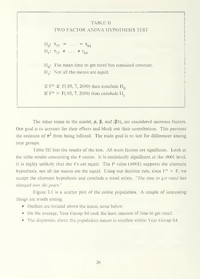
TABLE II

TWO FACTOR ANOVA HYPOTHESIS TEST

H : T77

= T84

H r T77

* . .•

* T84

H : The mean time to get rated has remained constant.

Ht

: Not all th c means are equal.

IFF :; < F(.95, 7, 2690) then conclude HQ

If F •: > F(.95, 7, 2690) then conclude H,

The other terms in the model, \i, p, and (Pi), are considered nuisance factors.

Our goal is to account for their effects and block out their contribution. This prevents

the estimate of <7" from being inflated. The main goal is to test for differences among

year groups.

Table III lists the results of the test. All main factors are significant. Look at

the table results concerning the t vector. It is statistically significant at the .0001 level.

It is highly unlikely that the %'s arc equal. The P value (.0001) supports the alternate

hypothesis, not all the means are the equal. Using our decision rule, since F* > F, we

accept the alternate hypothesis and conclude a trend exists. "The time to get rated has

changed over the years."

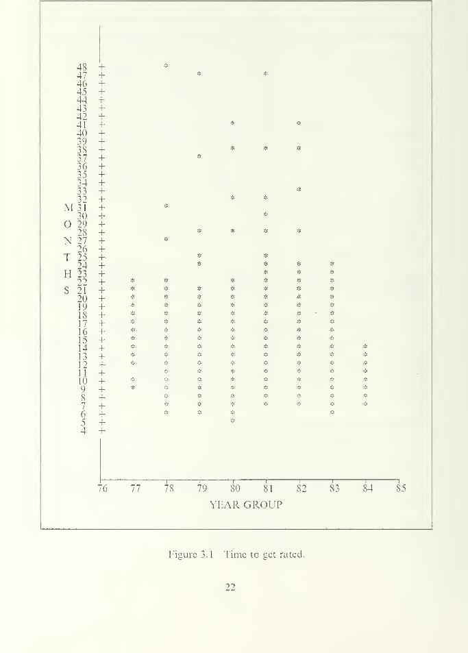
Figure 3.1 is a scatter plot of the entire population. A couple of interesting

things arc worth noting.

• Outliers are located above the mean, none below.

» On the average, Year Group 84 took the least amount of time to get rated.

• The dispersion about the population means is smallest within Year Group 84.

20

Notice the presence of outliers on the high side but none on the low side. As

expected, there is some minimum time required to get rated but no upper bound. We

will truncate all values of Y greater than 24 months in the ensuing analysis. The

reasons are threefold. One, as stated in the original set of objectives, the focus on

Basic Training will be restricted to the first two years of service. Two, a set of unusual

circumstances caused these individuals to take a substantial amount of time to get

rated. They have detoured from the expected training pipeline and we are not

interested in these individuals. Three, truncating the outliers will stabilize the variance

for future ANOVA tests. Only 25 data points will be lost. This amounts to .009 or

.9% of the observations. Censoring these data points should not affect future tests.

Now, let us look at 1984. Tables IV and V display Tukey's pairwise

comparisons for all year groups. All pairwise comparisons with year group S4 are

statistically significant. Since the average time to get rated by Year Group 84 is least

among all other year groups, we will delete that group from the ensuing analysis. No

further analysis need be done to that year group.

In summary, this first test establishes a trend. The time to get rated has

changed over the years. Secondly, the time to get rated has decreased from 19S3 to

1984. Let us investigate what happened prior to 1984.

2. Has the time to get rated increased or decreased through 1983?

The first test revealed the presence of a trend. The test also pointed out that

the time to get rated decreased from 1983 to 1984 for all groups. To see what

happened prior to 1984, we will test each group separately. We will follow the

methodology used in Neter, Wasserman, and Kutner [Ref. 2: Sec. 17.2]. The objectives

are:

8 Estimate the mean time to get rated for each year group.

• Test the means for statistical difference.

• Rank the means using a paired comparison test.

Our analytical tool to test the means for statistical differences is the Single F'actor

ANOVA Model. The Kruskal-Wallis (KW) nonparamctric test for equal means will be

used as a backup test. Then, given the means arc different, Tukey's paired comparison

test will be used to examine the nature of the differences. Based on the paired

comparison test results, we will rank the means.

21

48 +47 _j_

46 +45 +44 +43 +42 +41 +40 +39 +38 +37 +36 +35 +34 +33 +32 +

M 31 +30 -j-

29 +28 +

N 27 +26 +

T 25 +24 +

H 23 +22 +

S 21 +20 +19 +18 +17 +16 +15 +14 +13 +12 +11 +10 +9 +8 +7 +6 +5 +4 +

76 77 ^8 19 SO sT ~82 83~-i 1

84 S5

YEAR GROUP

Figure 3.1 Time to get rated.

22

TABLE III

TIME TO GET RATEDTWO FACTOR AXOVA RESULTS

CLASS LEVELS VALUES

P 3 AT AW AXT 8 77 78 79 80 81 82 83 84

s df SS MS F* PR>F*

Model 15 7310.0331 487.3355 34.51 0.0001

Error 2690 37984.2551 14.1205

Total 2705 45294.2882

S df SS MS p* PR>F*

P 2 247.7304 123.8652 8.77 0.0002

T 7 2844.0842 406.2977 28.77 0.0001

Pr 6 160.8890 26.8148 1.90 0.0774

R2 C.V. VMSE my

0.1614 23.1616 3.7577 16.2239

F(.95,7,l!690) = 2.01

23

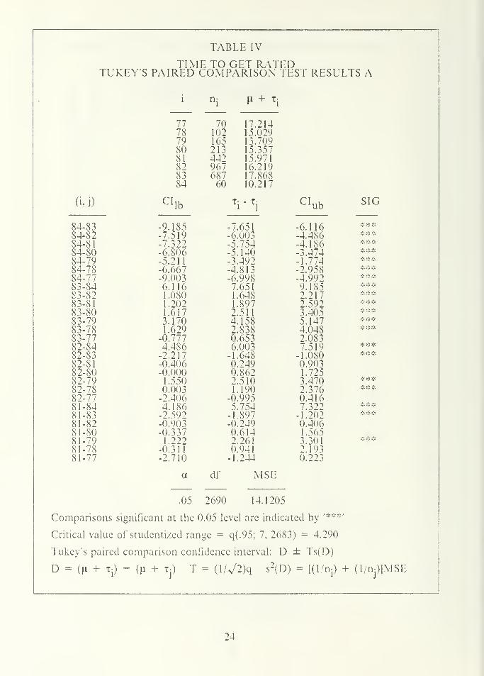
TABLE IV

TIME TO GET RATED i

TUKEY'S PAIRED COMPARISON TEST RESULTS A

• i

77

nj |i + x{

70 17.21478 102 15.02979 165 13.70980 213 15.35781 442 15.97182 967 16.21983 687 17.86884 60 10.217

G,j) CIlb

T- - T-1 J

CI ub SIG

84-83 -9.185 -7.651 -6.11684-82 -7.519 -6.003 -4.4S6

.». .'. .•-

84-81 -7.322 -5.754 -4.1S684-80 -6.806 -5.140 -3.474 -I"

•'.'• f,'

84-79 -5.211 -3.492 -1.77484-78 -6.667 -4.813 -2.958

y. >'. -•-

84-77 -9.003 -6.998 -4.992 •I' -!* *I*

83-84 6.116 7.651 9.185»•* .*j j«;

83-82 1.0S0 1.64S 2.217:.: :.: *

83-81 1.202 1.897 2.592:;-. .-;- :;-.

83-80 1.617 2.511 3.405 .;-. >:-. *

83-79 3.170 4.158 5.147 $ :-.: :•:

83-78 1.629 2.838 4.048 * .-;: *

83-77 -0.777 0.653 2.08382-84 4.4S6 6.003 7.519

.*. J. 4.

S2-83 -2.217 -1.648 -1.080^. ... .v

82-81 -0.406 0.249 0.90382-80 -0.000 0.862 1.72582-79 1.550 2.510 3.470 # :;-. *

82-78 0.003 1.190 2.37682-77 -2.406 -0.995 0.41681-S4 4.186 5.754 7.322

.'. -J. ;.'.

81-S3 -2.592 -1.897 -1.20281-82 -0.903 -0.249 0.40681-80 -0.337 0.614 1.56581-79 1.222 2.261 3.301

•!- :!» *.'

81-78 -0.311 0.941 2.19381-77 -2.710

a

.05

-1.244

df MSE

0.223

2690 14.1205

Comparisons signifiesint at the 0.05 level are indicated by '***'

Critical value of stuck:ntized range = q(.95; 7, 2683 ) = 4.290

Tukey's paircd comptirison con fidence interval: D ± Ts(D)

D = (ji + tj )- (|l + tj) T = (1/V2)q s

2(D) = Kl/n,) + (l/n|)]MSE

24

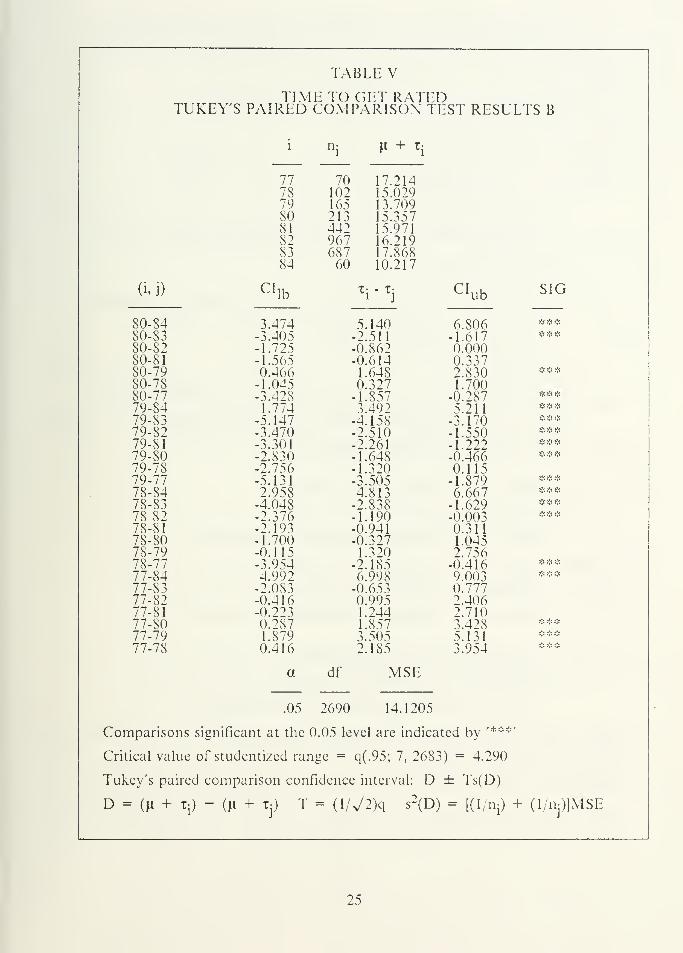
TABLE V

TIME TO GET RATEDTUKEY'S PAIRED COMPARISON TEST RESULTS B

i

77

nj n + tj

70 17.21478 102 15.02979 165 13.70980 213 15.35781 442 15.97182 967 16.21983 687 17.86884 60 10.217

(i,j) CIlb

T- - T-1 J

5.140

CI ub SIG

80-84 3.474 6.806 ***80-83 -3.405 -2.511 -1.617 ***80-82 -1.725 -0.862 0.00080-81 -1.565 -0.614 0.33780-79 0.466 1.648 2.830 ***80-7S -1.045 0.327 1.700SO-77 -3.428 -1.857 -0.287 ***79-84 1.774 3.492 5.211 ***79-83 -5.147 -4.158 -3.170 ***79-82 -3.470 -2.510 -1.550 ***79-81 -3.301 -2.261 -1.222 ***79-80 -2.830 -1.648 -0.466 ***79-78 -2.756 -1.320 0.11579-77 -5.131 -3.505 -1.879 ***78-84 2.958 4.813 6.667 ***78-83 -4.048 -2.838 -1.629 ***78 82 -2.376 -1.190 -0.003 ***78-81 -2.193 -0.941 0.31178-80 -1.700 -0.327 1.04578-79 -0.115 1.320 2.75678-77 -3.954 -2.185 -0.416 ***77-84 4.992 6.99S 9.003 ***77-83 -2.083 -0.653 0.77777-82 -0.4 1

6

0.995 2.40677-81 -0.223 1.244 2.71077-80 0.287 1.857 3.428 ***77-79 1.879 3.505 5.131 ***77-78 0.416

a

.05

2.185

df MSE

3.954 ***

2690 14.1205

Comparisons s ignific ant at the 0.05 level are indical:ed by

Critical value c f studentized range = q(.95; 7, 2683 )= 4.290

Tukcy's paired comp arison con fidence interval: D ± Ts(D)

D - (|l + T-) " (|l + Tj) T = (l/72)q s2(D) = [(1/nj) + (1/dj)]MSE

25

77 78 79 80 SI 82 83

AW Y"

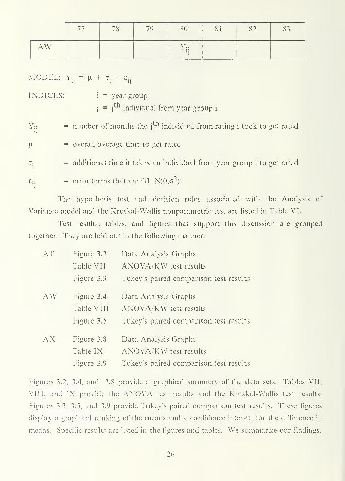
MODEL: Yij H + Tj

'ij

INDICES: i = year group

:th

Yii

j=

j individual from year group i

= number of months the j individual from rating i took to get rated

= overall average time to get rated

= additional time it takes an individual from year group i to get rated

= error terms that are iid N(0,cr2)

The hypothesis test and decision rules associated with the Analysis of

Variance model and the Kruskal-Wallis nonparametric test are listed in Table VI.

Test results, tables, and figures that support this discussion are grouped

together. They are laid out in the following manner.

AT Figure 3.2 Data Analysis Graphs

Table VII ANOVA/KW test results

Figure 3.3 Tukey's paired comparison test results

AW Figure 3.4 Data Analysis Graphs

Table VIII ANOVA/KW test results


AX Figure 3.8 Data Analysis Graphs

Table IX ANOVA/KW test results


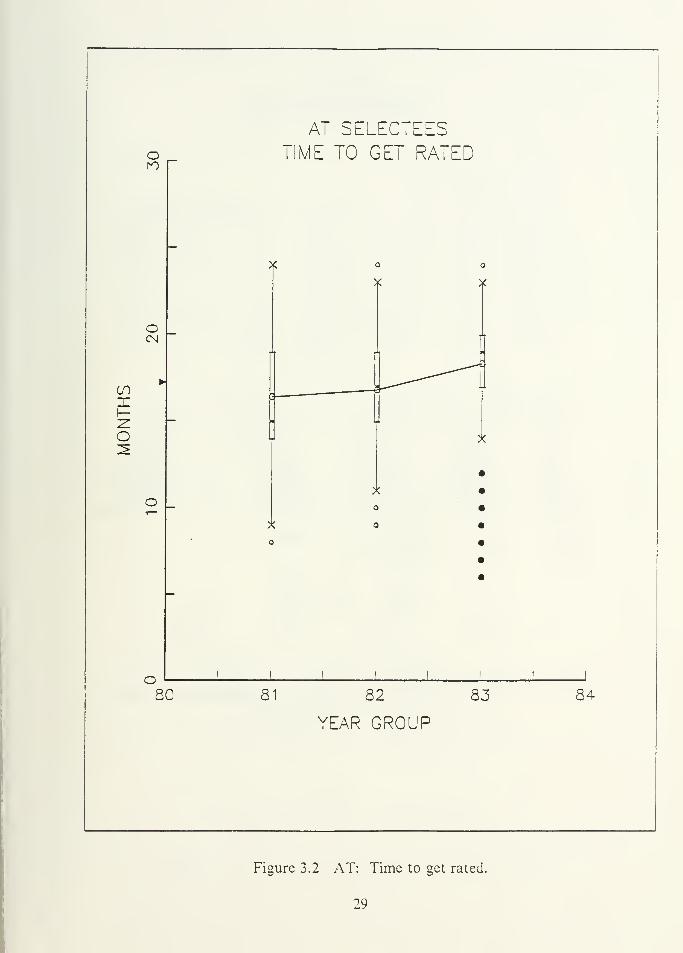
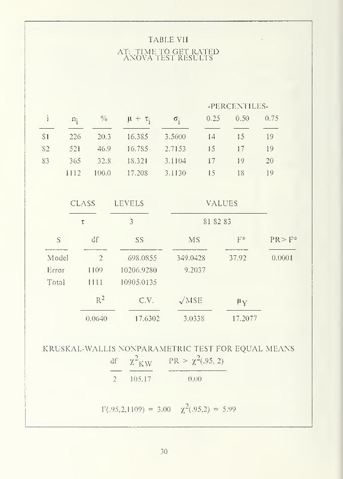
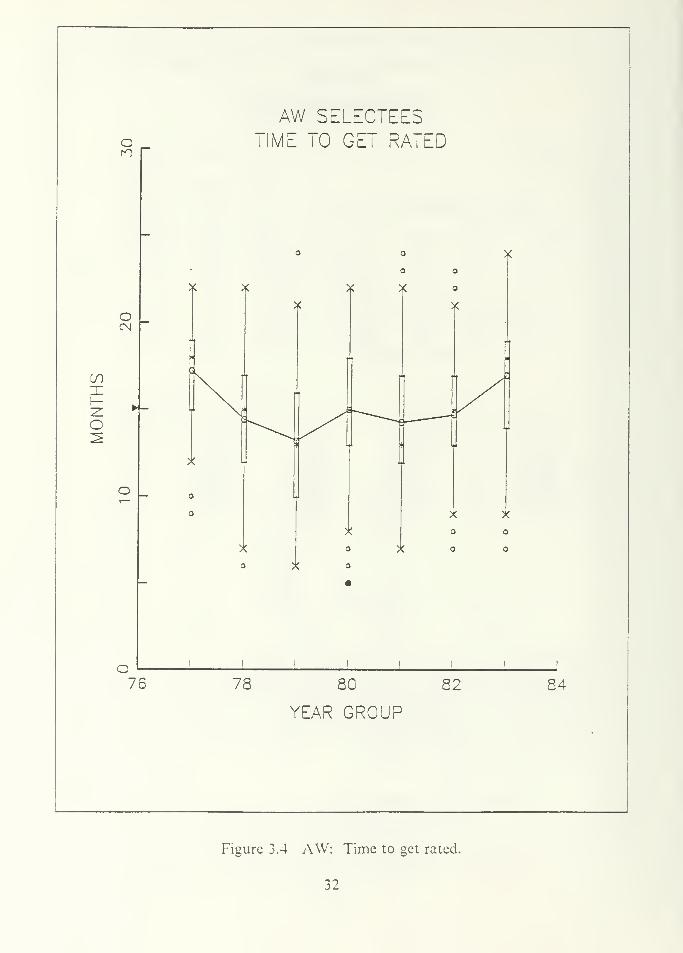
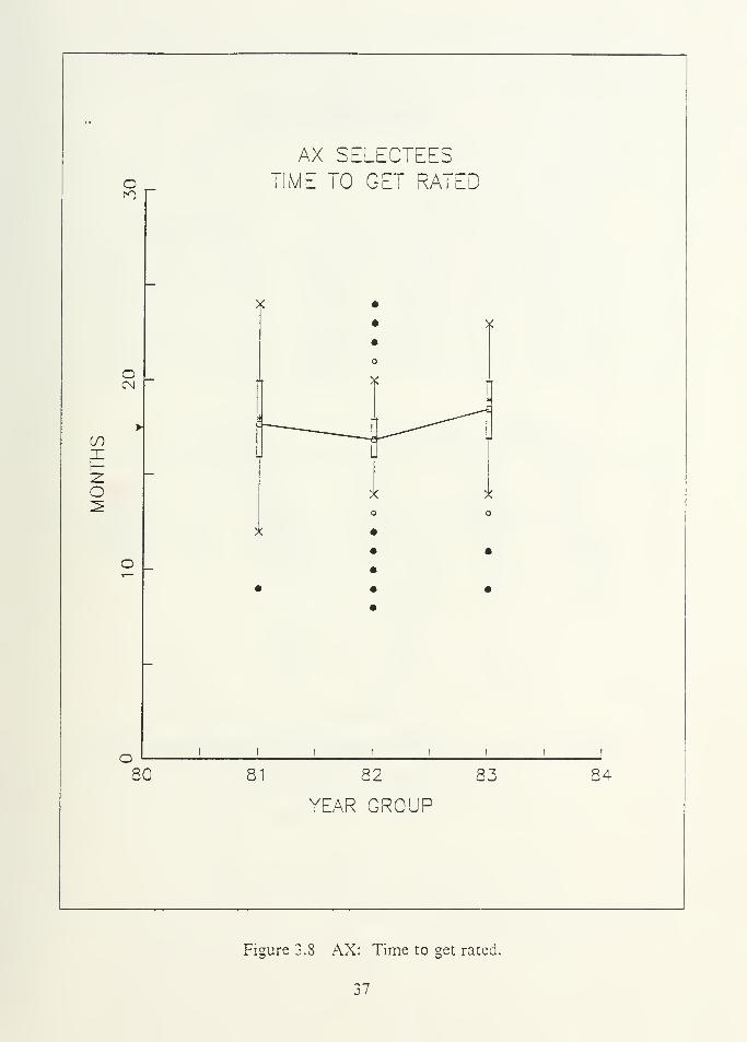
Figures 3.2, 3.4, and 3.S provide a graphical summary of the data sets. Tables VII,

VIII, and IX provide the ANOVA test results and the Kruskal-Wallis test results.

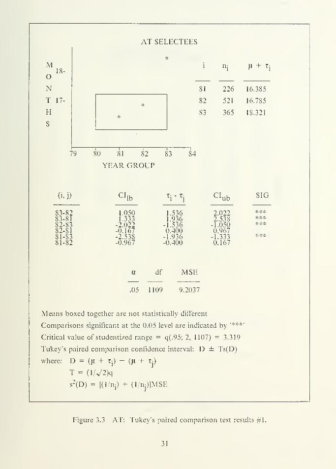
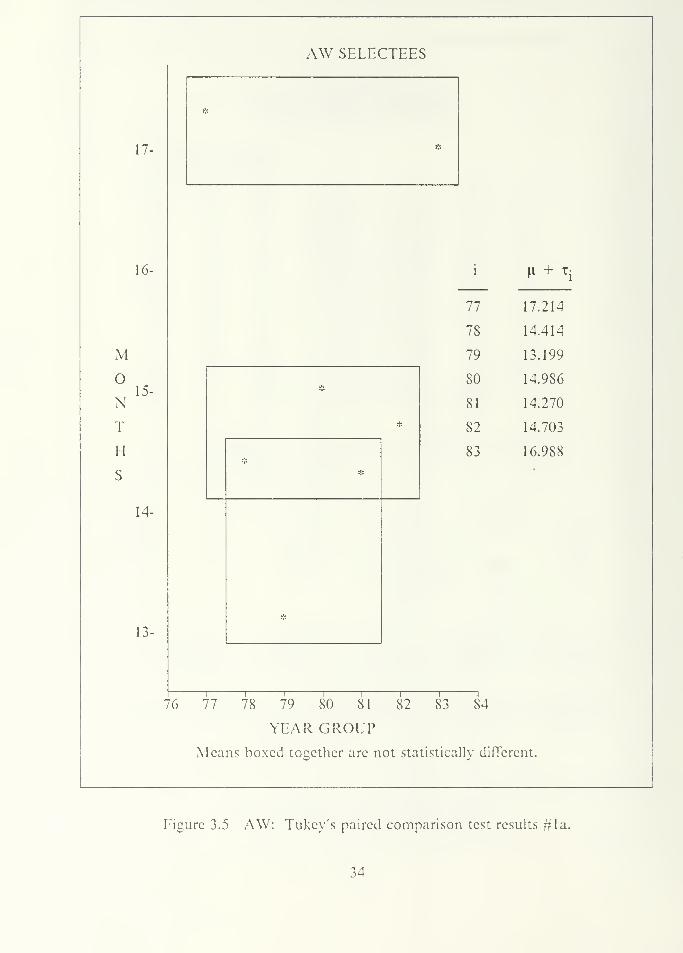
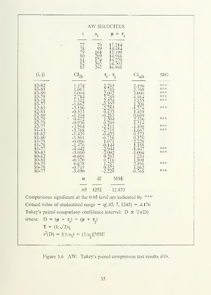
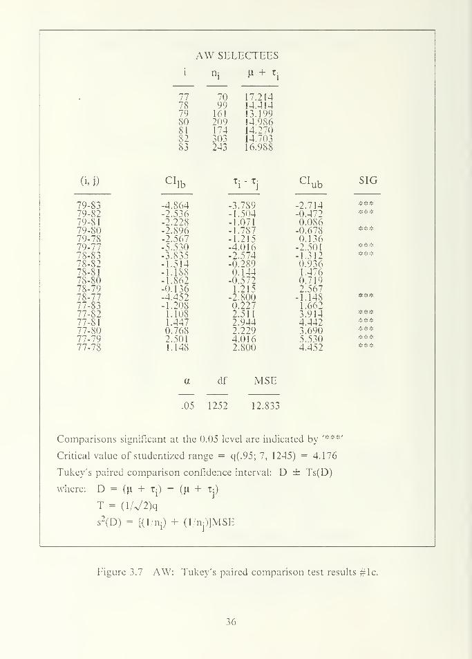
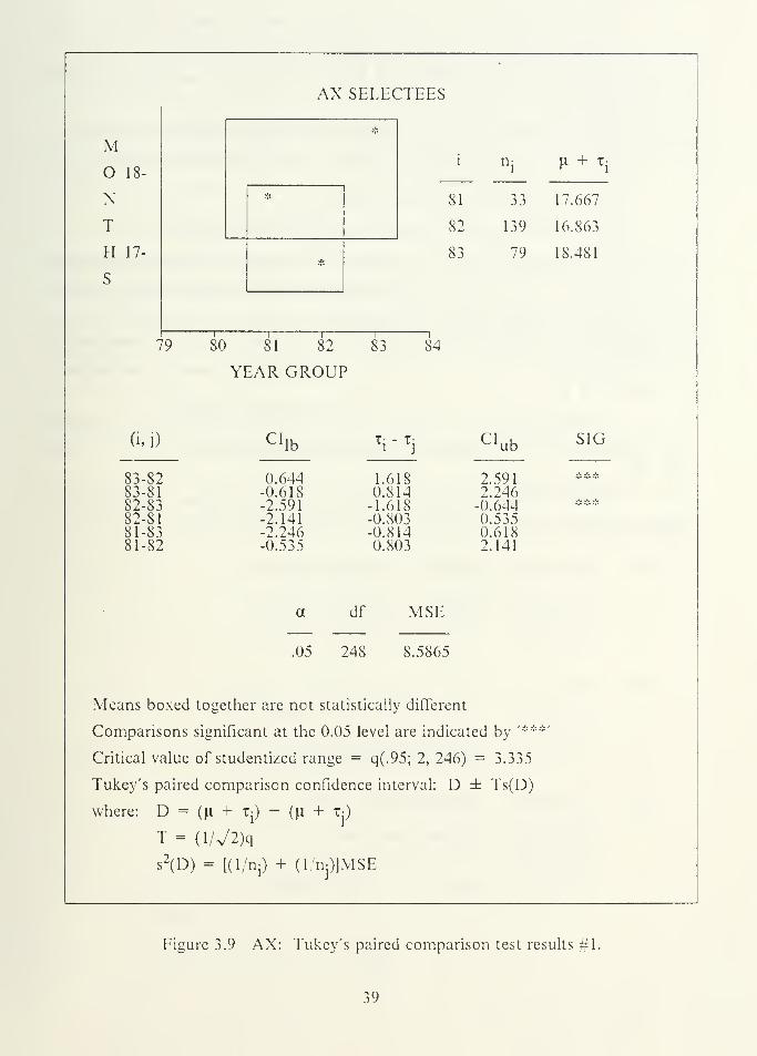
Figures 3.3, 3.5, and 3.9 provide Tukey's paired comparison test results. These figures

display a graphical ranking of the means and a confidence interval for the difference in

means. Specific results arc listed in the figures and tables. We summarize our findings.

26

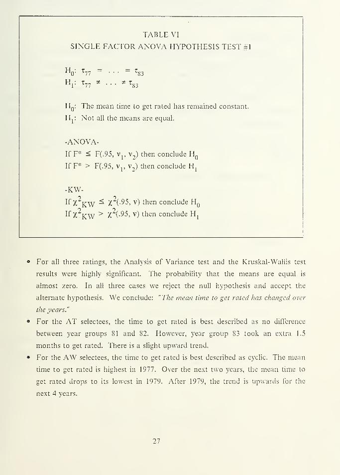
TABLE VI

SINGLE FACTOR ANOVA HYPOTHESIS TEST #1

HQ

: T77 *

• 'T83

Hr T77

X•

• • * T83

HQ

: The mean time to get rated has remained constant.

H r Not all the means are equal.

-ANOVA-

If F :* < F(.95, vp v

2)then conclude H

o

IfF : :: > F(.95, Vj, v2)

then conclude H,

-KW-

If X2KW ^ X

2(-95, v) then conclude H

Q

IfX2KW > X


l

For all three ratings, the Analysis of Variance test and the Kruskal-Wallis test

results were highly significant. The probability that the means are equal is

almost zero. In all three cases we reject the null hypothesis and accept the

alternate hypothesis. We conclude: "The mean time to get rated has changed over

the years."

For the AT selectees, the time to get rated is best described as no dilTcrcnce

between year groups 81 and 82. However, year group 83 took an extra 1.5

months to get rated. There is a slight upward trend.

For the AW selectees, the time to get rated is best described as cyclic. The mean

time to get rated is highest in 1977. Over the next two years, the mean time to

get rated drops to its lowest in 1979. After 1979, the trend is upwards for the

next 4 years.

27

• For the AX selectees, the trend is U shaped. The mean time to get rated drops

in 1982 and rises in 1983.

B. ATTRITION

Has attrition increased over the years? If the answer is yes, then attrition is a

factor causing training costs to rise. A simple relationship exists between attrition and

training costs. If the attrition rate is high, then the Navy must train more people to

fulfill quotas. Increasing the number of people to be trained raises the training cost.

Two methods are used to answer the question. The first method uses the actual

percent losses. The annual percent losses are inputs into the Cox and Stuart

nonparamctric test. The test determines whether an increasing trend exists. The

second method uses a regression approach. Attrition rates are estimated using a

nonlinear regression model. These rates serve as inputs into a simple linear regression

model.

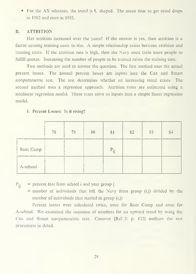
1. Percent Losses: Is it rising?

78 79 80 81 82 83 S4

Boot Camp pij

A-school

P-j = percent loss from school i and year groupj

= number of individuals that left the Navy from group (i,j) divided by the

number of individuals that started in group (i,j)

Percent losses were calculated twice, once for Boot Camp and once for

A-school. We examined the sequence of numbers for an upward trend by using the

Cox and Stuart nonparamctric test. Conover [Ref. 3: p. 133] outlines the test

procedures in detail.

28

AT SELECTEESo TIME TO GET RATED

X o <>

X X

OCN

i ÂX

o- I

X

o)

c

c «

1 4

> C 4

Q

4

i

! I !I

I 1 1

80 81 82 8.3 84

YEAR GROUP

Figure 3.2 AT: Time to get rated.

29

tl:

TABLE VII

AT: TIME TO GET RATEDANOVA TEST RESULTS

% H + Tj

-PERCENTILES-

0.25 0.50 0.75

81 82 83

81 226 20.3 16.385 3.5600 14 15 19

S2 521 46.9 16.785 2.7153 15 17 19

S3 365 32.8 18.321 3.1104 17 19 20

1112 100.0 17.208 3.1130 15 18 19

CLASS LEVELS VALUES

df SS

0.0640 17.6302

MS

Model 2 698.0855 349.0428

Error 1109 10206.9280 9.2037

Total 1111 10905.0135

R2 c.v. Vmse

3.0338

37.92

My

17.2077

PR>F

0.0001

KRUSKAL-WALLIS NONPARAMETRIC TEST FOR EQUAL MEANSdf 3C

2KW PR > X

2<- 95

'2 >

105.17 0.00

F(.95,2,1109) = 3.00 x (-95,2) = 5.99

30

AT SELECTEES

M18-

O

NT 17-

«•-

i

81

82

ni

226

521

]l + Tj

16.385

16.785-!-

H 83 365 18.321

S

-'9 80 81 82 S3 84

YEAR GROUP

(i,j) CIlb

1.536[.9361.536).4001.936).400

CI ub SIG

83-8283-8182-8382-8181-8381-82

1.0501.333

-2.022-0.167 (

-2.538-0.967 -(

2.0222.538-1.0500.967-1.3330.167

J, A ,*.

a df

.05 1109

MSE

J9.203'

Means boxed together are not statistically different

Comparisons significant at the 0.05 level are ind icated by '*** '

Critical value of studentized range = q(.95; 2, 1107 )= 3.319

Tukey's paired comparison confidence interval: D ± Ts(D)

where: D =(11 + X

{) -

(J! + T-)

T = (1/V2)q

s2(D )

- [(l/nj) + (l/n-)]MSE

Figure 3.3 AT: Tukey's paired comparison test results #1.

AW SELECTEESo TIME TO GET RATED

o o ;c

O O

Nc ; c C X o

OCM

>c

•

\C

—

£o

>

1

""*

^^^

o — -

> C )t

>* o e

>* o >lC o c

o 1C o

Q

- m

1 I 1 1 1 1 1!

76 78 80 82 84

YEAR GROUP

Figure 3.4 AW: Time to get rated.

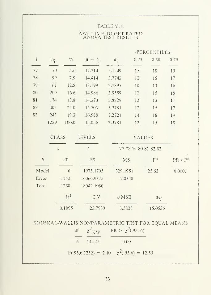
TABLE VIII

AW: TIME TO GET RATEDANOVA TEST RESULTS

-PERCENTILES-

i

77

ni

% H + Tj ai

0.25

15

0.50

18

0.75

1970 5.6 17.214 3.1249

78 99 7.9 14.414 3.7743 12 15 17

79 161 12.8 13.199 3.7895 10 13 16

80 209 16.6 14.986 3.9559 13 15 18

81 174 13.8 14.270 3.8829 12 13 17

82 303 24.0 14.703 3.2781 13 15 17

83 243 19.3 16.9SS 3.2721 14 18 19

1259 100.0 15.056 3.3781 12 15 18

CLASS LEVELS VALUES

T 7 77 78 79 80 81 82 83

S df SS MS F* PR>F*

Mode I 6 1975.1705 329.1951 25.65 0.0001

Error 1252 16066.9375 12.8330

Total 1258 18042.1080

R2 C.V. Vmse >lY

0.1095 23.7939 3.5823 15.0556

KRUSKAL-WALLIS NONPARAMETRIC TEST FOR EQUAL MEANSd

i

f X KW PR > x2(-?5, 6)

5 144.43 0.00

F(.95,6,1252) = 2. 10 X2(-95,6) = 12.59

33

AW SELECTEES

17-

16-

MO

NT

H

S

15-

14-

13-

r':

•fc

*

*

fi + tj

77 17.214

78 14.414

79 13.199

80 14.9S6

81 14.270

S2 14.703

83 16.988

76 ~T1 78 79 80 I\ 82 83 84

YEAR GROUPMeans boxed together arc not statistically different.

Figure 3.5 AW: Tukey's paired comparison test results #la.

34

AW SELECTEES

i

77

ni >

l + Ti

70 17.21478 99 14.41479 161 13.19980 209 14.98681 174 14.27082 303 14.70383 243 16.988

(i,j) CIlb

x- - X-i

J

2.285

CI ub SIG

83-82 1.374 3.196 ***83-81 1.667 2.718 3.768 ***83-80 1.004 2.002 3.000 ***83-79 2.714 3.789 4.864 ***83-78 1.312 2.574 3.835 ***83-77 -1.662 -0.227 1.20882-83 -3.196 -2.285 -1.374 ***82-81 -0.573 0.433 1.43982-80 -1.234 -0.283 0.66982-79 • 0.472 1.504 2.536 ***82-78 -0.936 0.289 1.51482-77 -3.914 -2.511 -1.108 ***81-83 -3.768 -2.718 -1.667 ***81-82 -1.439 -0.433 0.57381-80 -1.801 -0.716 0.37081-79 -0.0S6 1.071 2.22881-78 -1.476 -0.144 1.18881-77 -4.442 -2.944 -1.447 ***80-83 -3.000 -2.002 -1.004 ***80-82 -0.669 0.283 1.23480-81 -0.370 0.716 1.80180-79 0.678 1.787 2.896 ***80-78 -0.719 0.572 1.86280-77 -3.690 -2.229 -0.768 ***

a

.05

df MSE

1252 12.833

Comparisons significant at the 0.05 level are indica ted by

Critical value of studentized range = q(.95; 7, 1245) = 4.176

Tukey's paired comparison confidence interval: D ± Ts(D)

where: D =(H + tj) - (|i + Tj)

T = (1/V2)q

s2(D) == [(l/ni) + (1, n:)]MSE

Figure 3.6 AW: Tukey's paired comparison test results # lb.

35

AW SELECTEES

i

77

nj |i- + tj

70 17.21478 99 14.41479 161 13.19980 209 14.98681 174 14.27082 303 14.70383 243 16.9S8

(i,j) CIlb

T- - T-1 J

-3.7S9

CI ub SIG

79-83 -4.864 -2.714 ***79-82 -2.536 -1.504 -0.472 :::::: *

79-81 -2.228 -1.071 0.08679-80 -2.896 -1.787 -0.678 ***79-78 -2.567 -1.215 0.13679-77 -5.530 -4.016 -2.501 *»*78-83 -3.835 -2.574 -1.312 ***78-82 -1.514 -0.289 0.9367S-81 -1.188 0.144 1.47678-80 -1.862 -0.572 0.71978-79 -0.136 1.215 2.56778-77 -4.452 -2.800 -1.148 ***77-83 -1.208 0.227 1.66277-82 1.108 2.511 3.914 ***77-81 1.447 2.944 4.442 ***77-80 0.768 2 9 29 3.690 ***77-79 2.501 4i016 5.530 ***77-78 1.148

a

.05

2.800

df MSE

4.452 ***

1252 12.833

Comparisons significant at the 0.05 level are indica ted bv '***'

Critical value of studentized range = q(.95; 7, 1245) = 4.176

Tukey's paircd compai"ison confidence interval: D ± Ts(D)

where: D =(H +

î )" (|i + T

PT = (1/V2)q

s2(D) --

l(i;ni)+ (1, n:)]MSE

Figure 3.7 AW: Tukey's paired comparison test results #lc.

36

AX SELECT EESo TIME T( GET RATEDro

o

inxi—~ZL

O

80

xo

81 82

YEAR GROUP

83 84

Figure 3.8 AX: Time to get rated.

37

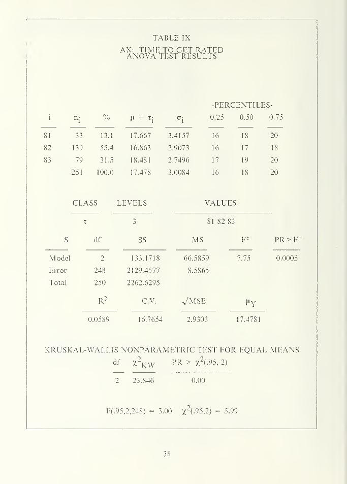
TABLE IX

AX: TIME TO GET RATEDANOVA TEST RESULTS

-PERCENTILES-

i ni

33

% H + x{

ffi

0.25

16

0.50

18

0.75

81 13.1 17.667 3.4157 20

82 139 55.4 16.863 2.9073 16 17 18

83 79 31.5 18.481 2.7496 17 19 20

251 100.0 17.478 3.0084 16 IS 20

CLASS LEVELS VALUES

3 81 82 83

elf SS MS F* PR>F

Model 9 133.1718 66.5859

Error 248 2129.4577 8.5865

Total 250 2262.6295

R2 C.V. VMSE

7.75 0.0005

my

0.0589 16.7654 2.9303 17.47S1

KRUSKAL-WALLIS NONPARAMETRIC TEST FOR EQUAL MEANSdf X

2KW PR > X

2(-95, 2)

23.846 0.00

F(. 95,2,248) = 3.00 -/2(.95,2) = 5.99

38

M

AX SELECTEES

*

O 18-

N

i

81

ni

33

|1 + Tj

* 17.667

T

H 17-

82 139

79

16.863

1S.4S1* 83

S

;'9 SO 81 82 83 84

YEAR GROUP

(i,j) CIlb

T- - T-i

3

1.6180.814-1.618-0.803-0.8140.803

CI ub SIG

83-8283-8182-8382-8181-8381-82

0.644-0.618-2.591-2.141-2.246-0.535

2.5912.246-0.6440.5350.6182.141

***

a df

.05 24S

MSE

8.5865

Means boxed together are not statistically different

Comparisons significant at the 0.05 level are indicated by '*** '

Critical value of studcntizcd range = q(.95; 2, 246) = 3.335

Tukey's paire d comparison confidence interval: D ± Ts(D)

where: D = (|l + tj) - (|i + tj)

T = (l/v/2)q

s2(D) = = [(1/nj) + (l/nj)]MSE

Figure 3.9 AX: Tukey's paired comparison test results #{.

39

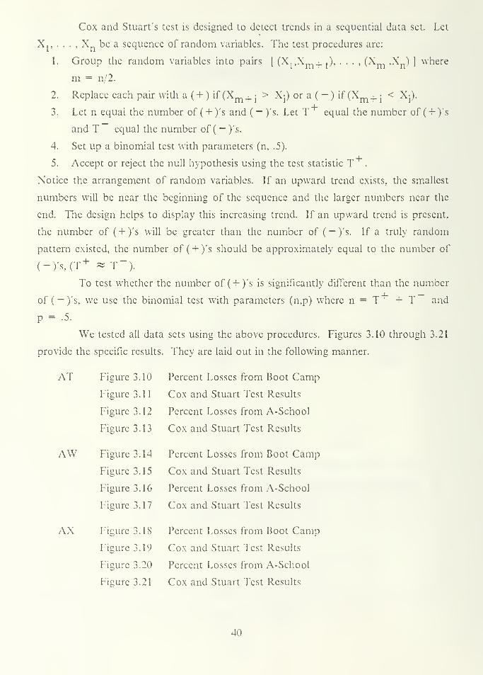
Cox and Stuart's test is designed to detect trends in a sequential data set. Let

Xj, . . . , Xn be a sequence of random variables. The test procedures arc:

1. Group the random variables into pairs [ (X,,Xm+ .), . . .,(Xm ,Xn) ] where

m = n/2.

2. Replace each pair with a ( + ) if (X +- > X-) or a ( -) if (Xm+i < Xj).

3. Let n equal the number of ( + )'s and (— )'s. Let T equal the number of ( + )'s

and T equal the number of (— )'s.

4. Set up a binomial test with parameters (n, .5).

5. Accept or reject the null hypothesis using the test statistic T .

Notice the arrangement of random variables. If an upward trend exists, the smallest

numbers will be near the beginning of the sequence and the larger numbers near the

end. The design helps to display this increasing trend. If an upward trend is present.

the number of ( + )'s will be greater than the number of (— )'s. If a truly random

pattern existed, the number of ( + )'s should be approximately equal to the number of

(-)'s,(T+ * T").

To test whether the number of ( + )'s is significantly different than the number

of ( — )'s, we use the binomial test with parameters (n,p) where n = T + T and

p = .5.

We tested all data sets using the above procedures. Figures 3.10 through 3.21

provide the specific results. They are laid out in the following manner.

AT Figure 3.10 Percent Losses from Boot Camp

Figure 3.11 Cox and Stuart Test Results

Figure 3.12 Percent Losses from A-School


AW Figure 3.14 Percent Losses from Boot Camp




AX Figure 3.18 Percent Losses from Boot Camp




40

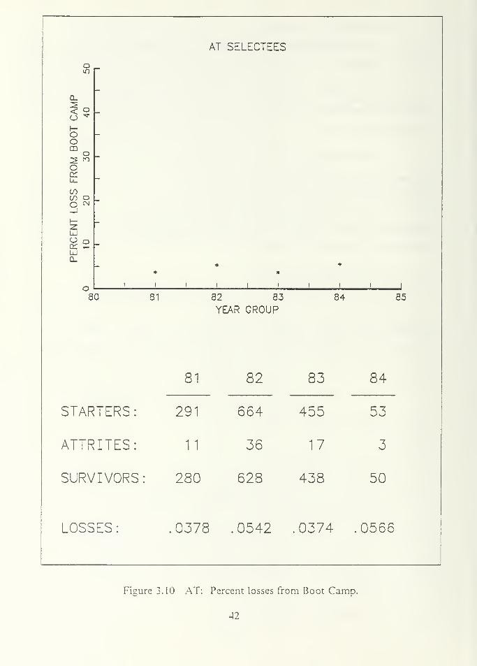
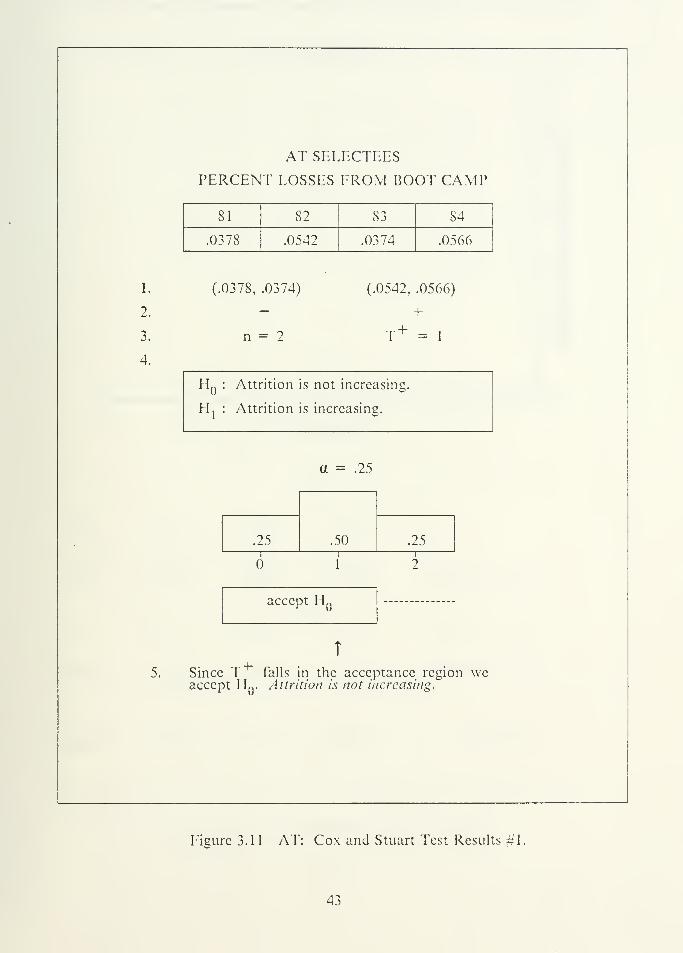
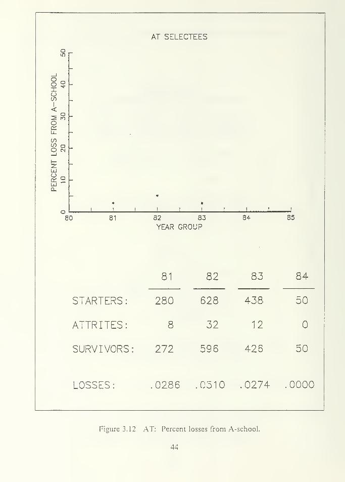
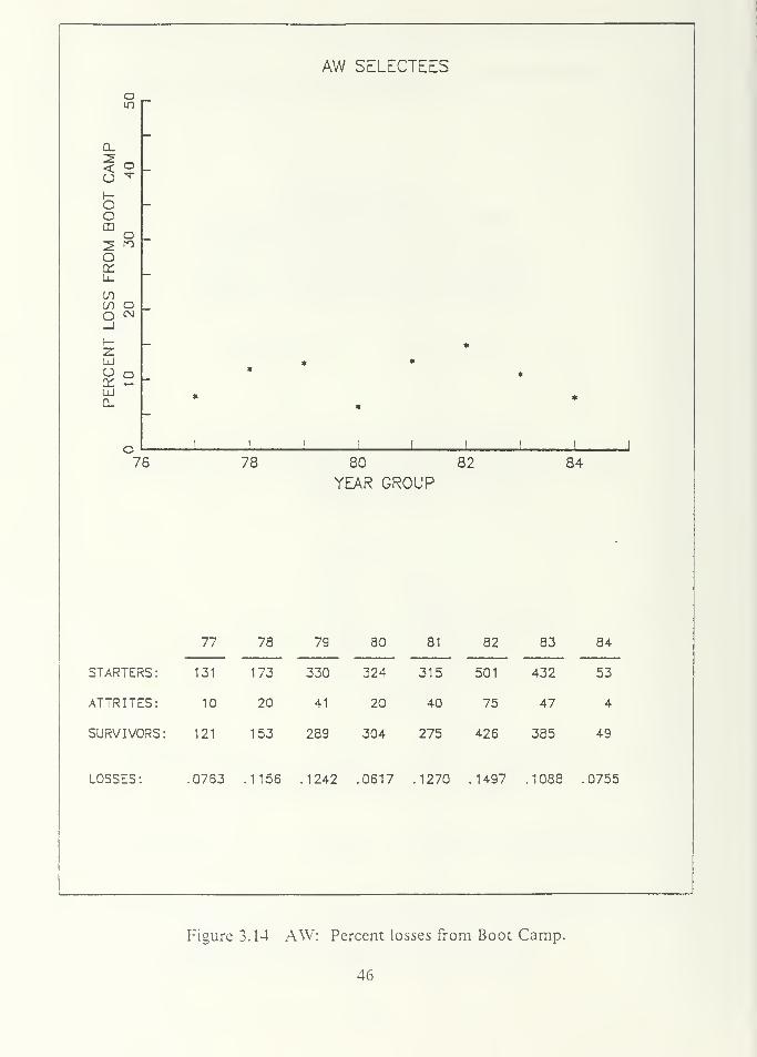
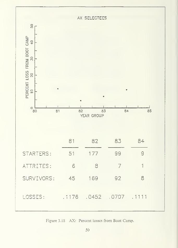
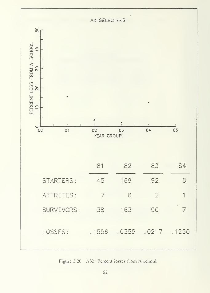
Figures 3.10, 3.14, and 3. IS graphically display the percent losses from Boot Camp.

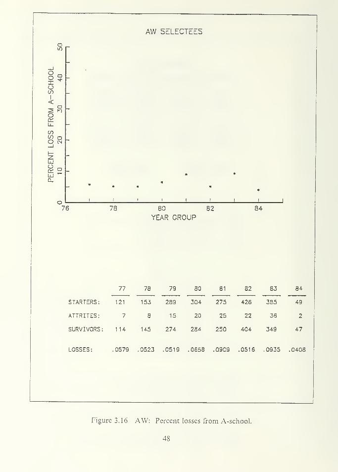
Similarly, Figures 3.12, 3.16, and 3.20 graphically display the percent losses from

A-school. Figures 3.11, 3.15, and 3.19 provide the Cox and Stuart test results for data

sets pertaining to Boot Camp. Similarly Figures 3.13, 3.17, and 3.21 provide the Cox

and Stuart test results for attrition losses in A-school. In all cases, we accepted the

null hypothesis; Attrition is not increasing.

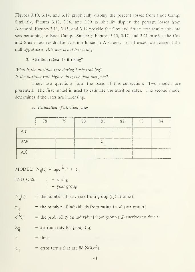
2. Attrition rates: Is it rising?

What is the attrition rate during basic training!

Is the attrition rate higher this year than last year?

These two questions form the basis of this subsection. Two models are

presented. The first model is used to estimate the attrition rates. The second model

determines if the rates arc increasing.

a. Estimation of attrition rates

78 79 80 81 82 83 S4

AT

AW hAX

MODEL: N»(t) = n-e'îj1 + E-

INDICES:

Nij(t)

ehf

H

j= year group

= the number of survivors from group (i,j) at time t

= the number of individuals from rating i and year groupj

= the probability an individual from group (i,j) survives to time t

= attrition rate for group (i,j)

= time

= error terms that arc iid N(0,(T )

41

AT SELECTEES

o

FROM

BOOT

30

COin N -

PERCENT

)

10

* *

i i i i

*

1 1

80 81 82 83

YEAR GROUP84 85

STARTERS:

81 82 83 84

291 664 455 53

ATTRITES: 11 36 17 3

SURVIVORS: 280 628 438 50

LOSSES: .0378 .0542 .0374 .0566

Figure 3.10 AT: Percent losses from Boot Camp.

42

AT SELECTEES

PERCENT LOSSES FROM BOOT CAMP

81 82 83 84

.0378 .0542 .0374 .0566

1.

2.

3.

4.

(.0378, .0374)

n = 2

(.0542, .0566)

+

T + = 1

HQ

: Attrition is not increasing.

H, : Attrition is increasing.

a = .25

T

.+

.50.25 .25i

1

i

2

,. WQ

Since T falls in the acceptance region weaccept IL. Attrition is not increasing.

Figure 3.1 1 AT: Cox and Stuart Test Results #1.

43

AT SELECTEES

o

-SCHOOL

40 -

FROM

A-

30 -

COCO oO CN_l

PERCENT

10 -

*

*

I I !

*

i i i i ii

i

80 81 82 83

YEAR GROUP84 85

STARTERS:

81 82 83 84

280 628 438 50

ATTRITES: 8 32 12

SURVIVORS: 272 596 426 50

LOSSES: .0286 .0510 .0274 .0000

Figure 3.12 AT: Percent losses from A-school.

44

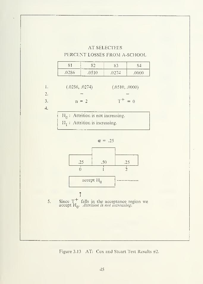
AT SELECTEES

PERCENT LOSSES FROM A-SCHOOL

81 82 83 84

.0286 .0510 .0274 .0000

1.

2.

3.

4.

(.0286, .0274) (.0510, .0000)

T ' =

EL : Attrition is not increasing.

II j : Attrition is increasing.

a = .25

.25 .50 .25

accept Hq

T

-r+Since T falls in the acceptance region weaccept EL. Attrition is not increasing.

Figure 3.13 AT: Cox and Stuart Test Results #2.

45

78 80 82

YEAR GROUP84

77 78 79 80 81 82 83 84

STARTERS

:

131 173 330 324 315 501 432 53

ATTRITES: 10 20 41 20 40 75 47 4

SURVIVORS: 121 153 289 304 275 426 385 49

LOSSES: ,0763 .1156 .1242 .0617 .1270 .1497 .1088 .0755

Figure 3.14 AW: Percent losses from Boot Camp.

46

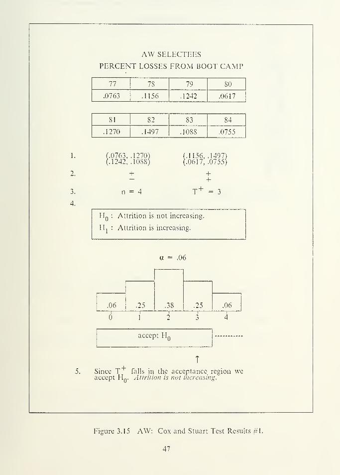
AW SELECTEES


77 7S 79 80

.0763 .1156 .1242 .0617

81 82 83 84

.1270 .1497 .1088 .0755

1.

2.

3.

4.

(.0763, .1270(.1242, .1088

1 !

+

n = 4

1156, .1497)0617, .0755)

++

T + = 3

HQ


PL : Attrition is increasing.

a = .06

.38.25 .25.06 .06

.+

accept PL

T

Since T falls in the acceptance region weaccept PL. Attrition is not increasing.

Picure 3.15 AW: Cox and Stuart Test Results #1.

47

80 82

YEAR GROUP

77 78 79 80 81 82 83 84

STARTERS: 121 153 289 304 275 426 385 49

ATTRITES: 7 a 15 20 25 22 36 2

SURVIVORS: 114- 145 274 28* 250 404 349 47

LOSSES: ,0579 .0523 .0519 .0658 .0909 .0516 .0935 .0408

Figure 3.16 AW: Percent losses from A-school.

48

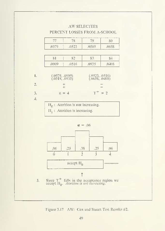
AW SELECTEES

PERCENT LOSSES FROM A-SCHOOL

77 78 79 80

.0579 .0523 .0519 .065S

SI 82 S3 84

.0909 .0516 .0935 .0408

1.

2.

3.

4.

.0579, .0909)

.0519, .0935)

n = 4

.0523, .0516)

.0658, .0408)

r + = 2

HQ


ITj : Attrition is increasing.

a = .06

.38i

.25i

.25i

.06i

.061—^—

I

.+

accept I

L

T

Since T falls in the acceptance region weaccept IL. Auriiion is not increasing."

Figure 3.17 AW; Cox and Stuart Test Results #2.

49

AX SELECTEES

o

Q_

FROM

BOOT

30 -

COCO oo w

PERCENT

)

10

*

I !

*

*III! i i

i j

80 81 82 83

YEAR GROUP84 85

STARTERS:

81 82 83 84

51 177 99 9

ATTRITES: 6 8 7 1

SURVIVORS: 45 169 92 8

LOSSES: .1176 .0452 .0707 .1111

Figure 3.18 AX: Percent losses from Boot Camp.

50

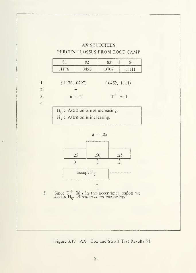
AX SELECTEES


SI 82 S3 84

.1176 .0452 .0707 .1111

(.1176, .0707)

n = ?

(.0452, .1111)

+

HQ


Hj : Attrition is increasing.

a = .25

.50i

.25i

.25i

accept LL

T

.+Since T falls in the acceptance region weaccept I L. Attrition is not increasing.

Figure 3.19 AX: Cox and Stuart Test Results #1.

51

AX SELECTEES

o

-SCHOOL

40

PROM

A-

30

COCO oO CN_1

-

PERCENT

)

10

•

-

i

i

i«III!

«

i

80 81 82 83

YEAR GROUP84 85

STARTERS:

81 82 83 84

45 169 92 8

ATTRITES: 7 6 2 1

SURVIVORS: 38 163 90 7

LOSSES: .1556 .0355 .0217 .1250

Figure 3.20 AX: Percent losses from A-school.

52

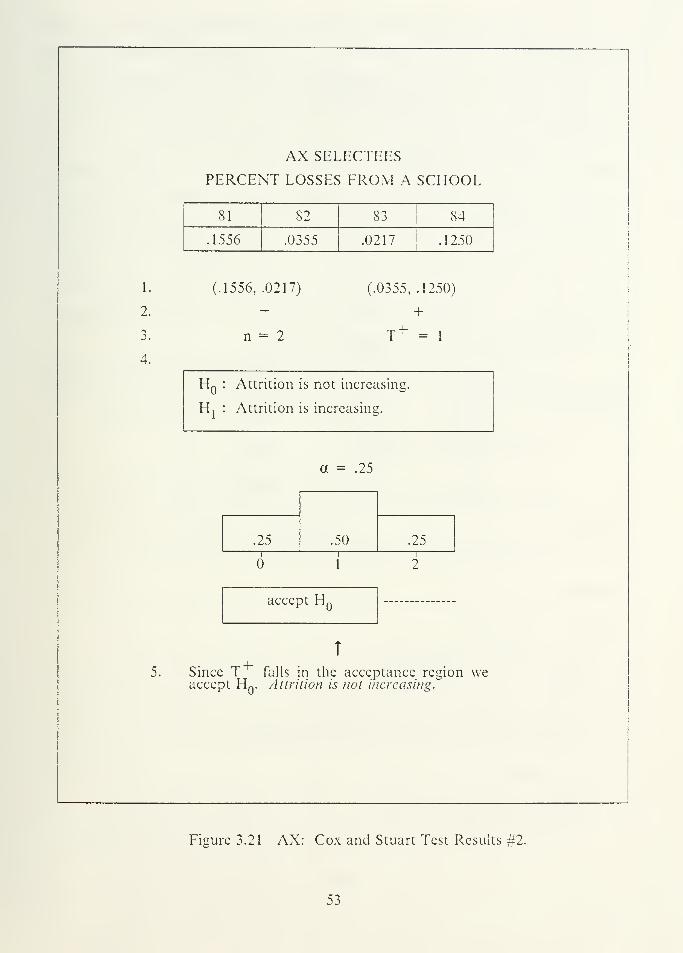
AX SELECTEES

PERCENT LOSSES FROM A SCHOOL

81 S2 83 84

.1556 .0355 .0217 .1250

1.

2.

3.

4.

(.1556, .0217)

n = 2

(.0355, .1250)

+

T + =l

HQ


Hj : Attrition is increasing.

.25

a = .25

.50 .25

5.

accept LL

T

.+Since T falls in the acceptance region weaccept H

Q. Attrition is not increasing.

Figure 3.21 AX: Cox and Stuart Test Results #2.

53

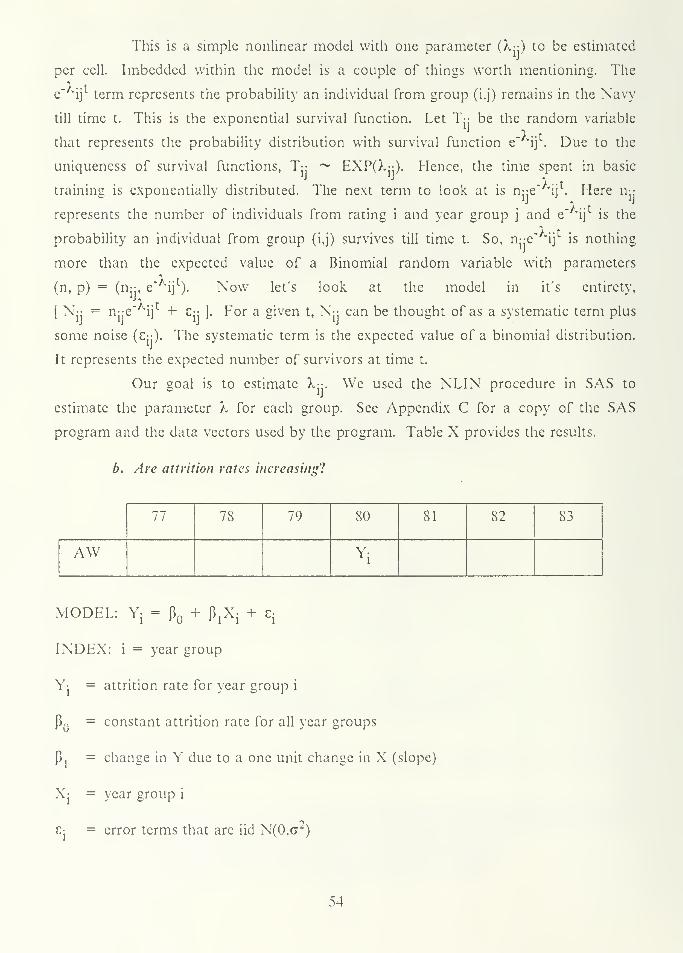
This is a simple nonlinear model with one parameter (k--) to be estimated

per cell. Imbedded within the model is a couple of things worth mentioning. The

e ij term represents the probability an individual from group (i.j) remains in the Navy

till time t. This is the exponential survival function. Let T-: be the random variable

that represents the probability distribution with survival function e ij . Due to the

uniqueness of survival functions, T- ~ EXP(X-:). Hence, the time spent in basic

training is exponentially distributed. The next term to look, at is n--e" ijr

. Mere n-:

represents the number of individuals from rating i and year group j and c ij1

is the

probability an individual from group (i,j) survives till time t. So, n-e ij is nothing

more than the expected value of a Binomial random variable with parameters

(n, p) = (n-:, e ij1). Now let's look at the model in it's entirety,

[ N- = n-e ij + c- ]. For a given t, N- can be thought of as a systematic term plus

some noise (£-). The systematic term is the expected value of a binomial distribution.

It represents the expected number of survivors at time t.

Our goal is to estimate X--. We used the NLIN procedure in SAS to

estimate the parameter X for each group. See Appendix C for a copy of the SAS

program and the data vectors used by the program. Table X provides the results.

b. Are attrition rates increasing!

77 78 79 80 81 82 83

AW Yi

MODEL: Yj = p + p1

Xi

+ z[

INDEX: i = year group

Y: = attrition rate for year group i

{L = constant attrition rate for all year groups

p, = change in Y due to a one unit change in X (slope)

X: = year group i

C: = error terms that arc iid N(0,(72)

54

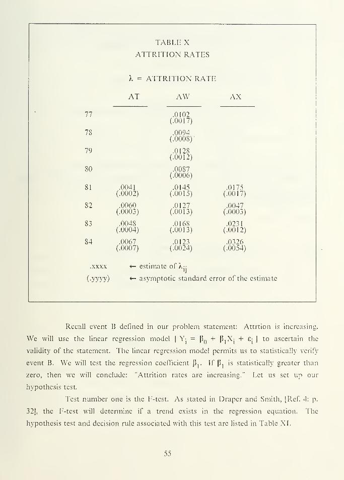
TABLE X

ATTRITION RATES

X = ATTRITION RATE

77

AT AW AX

.0102(.0017)

78 .0094(.0008)'

79 .0128(.0012)

80 .0087(.0006)

81 .0041(.0002)

.0145(.0015)

.0175(.0017)

82 .0060(.0003)

.0127(.0013)

.0047(.0003)

83 .0048(.0004)

.0168(.0013)

.023

1

(.0012)

84 .0067(.0007)

.0123(.0024)

.0326(.0054)

.xxxx «- estimate of X-

(•yyyy) «- asymptotic standard error of the estimate

Recall event B defined in our problem statement: Attrtion is increasing.

We will use the linear regression model [ Y- = p + (LjXj + c- ] to ascertain the

validity of the statement. The linear regression model permits us to statistically verify

event B. We will test the regression coefficient pj. If pj is statistically greater than

zero, then we will conclude: 'Attrition rates are increasing." Let us set up our

hypothesis test.

Test number one is the F-tcst. As stated in Draper and Smith, [Ref. 4: p.

32J, the F-tcst will determine if a trend exists in the regression equation. The

hypothesis test and decision rule associated with this test are listed in Table XL

55

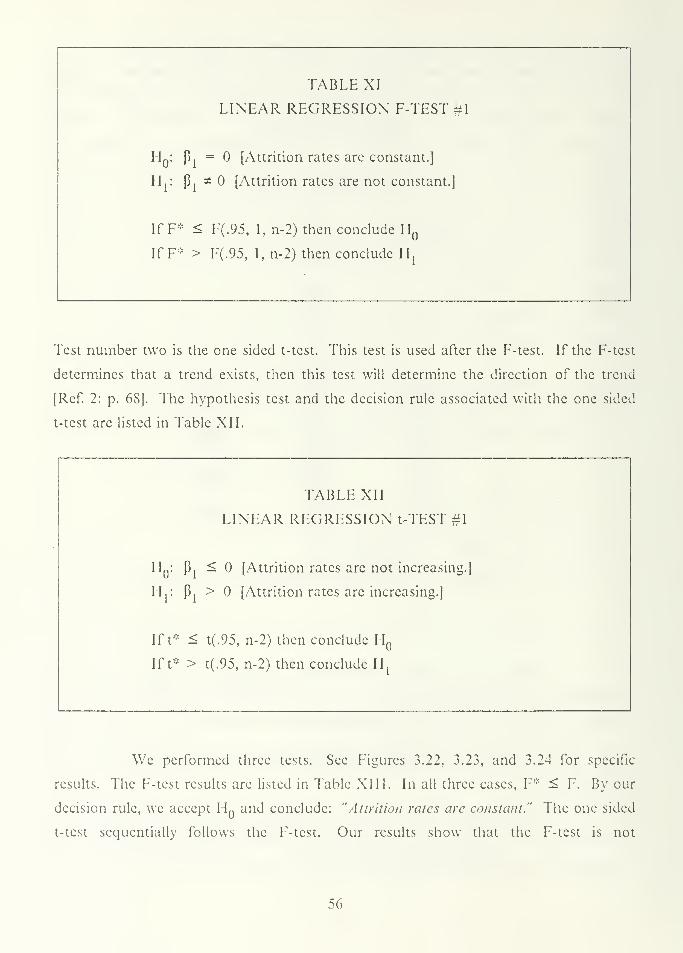
TABLE XI

LINEAR REGRESSION F-TEST #1

l\Q

: P1

= [Attrition rates are constant.]

H,: p1* [Attrition rates are not constant.]

If F* < F(.95, 1, n-2) then conclude HQ

If F* > F(.95, I, n-2) then conclude H{

Test number two is the one sided t-test. This test is used after the F-test. If the F-test

determines that a trend exists, then this test will determine the direction of the trend

[Ref. 2: p. 68]. The hypothesis test and the decision rule associated with the one sided

t-test are listed in Table XII.

TABLE XII

LINEAR REGRESSION t-TEST#1

H„: Pi< [Attrition rates are not increasing.]

H,: P. > [Attrition rates are increasing.]

ir t-: < t(.95 n-2) then conclude H

iff > t(.95, n-2) then conclude H,

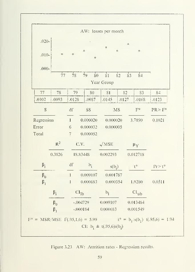
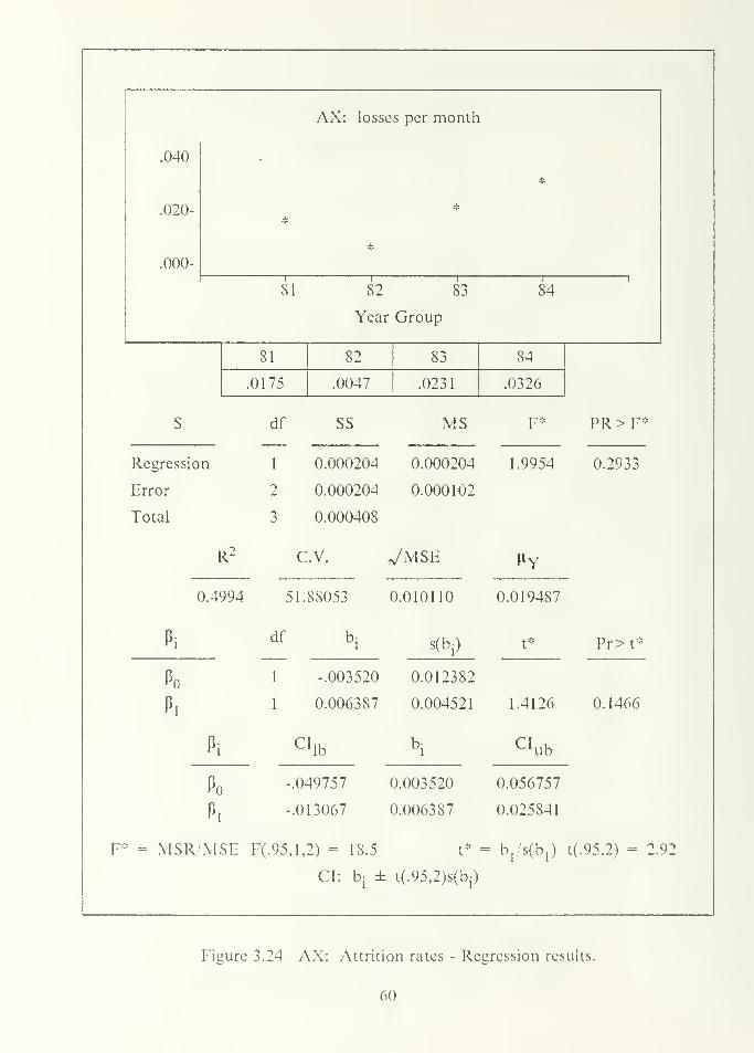
We performed three tests. See Figures 3.22, 3.23, and 3.24 for specific

results. The F-test results are listed in Table XI II. In all three cases, F* ^ F. By our

decision rule, we accept I-L and conclude: "Attrition rates are constant." The one sided

t-test sequentially follows the F-tcst. Our results show that the F-test is not

56

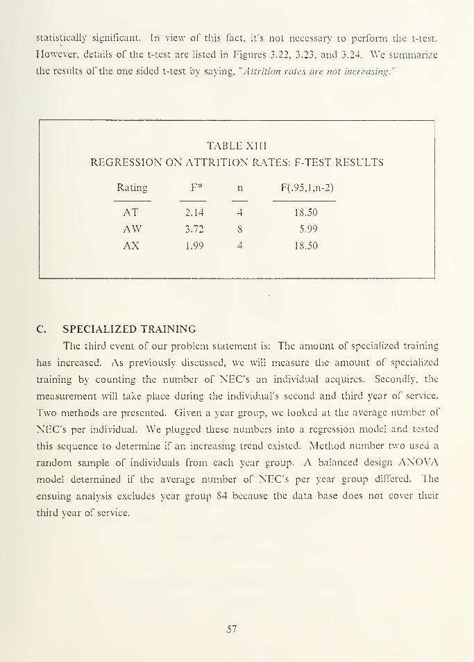
statistically significant. In view of this fact, it's not necessary to perform the t-test.

However, details of the t-test are listed in figures 3.22, 3.23, and 3.24. We summarize

the results of the one sided t-test by saying, "Attrition rates are not increasing."

TABLE XIII

REGRESSION ON ATTRITION RATES: F-TEST RESULTS

Rating F* n F(.95,l,n-2)

AT

AWAX

2.14 4 18.50

3.72 8 5.99

1.99 4 18.50

C. SPECIALIZED TRAINING

The third event of our problem statement is: The amount of specialized training

has increased. As previously discussed, we will measure the amount of specialized

training by counting the number of NEC's an individual acquires. Secondly, the

measurement will take place during the individual's second and third year of service.

Two methods are presented. Given a year group, we looked at the average number of

NEC's per individual. We plugged these numbers into a regression model and tested

this sequence to determine if an increasing trend existed. Method number two used a

random sample of individuals from each year group. A balanced design ANOVAmodel determined if the average number of NEC's per year group differed. The

ensuing analysis excludes year group 84 because the data base does not cover their

third year of service.

57

AT: losses per month

.008-

sfc

**

.004-y<

.000-

81 82 83 84i

Year Group

81 82 S3 S4

.0041 .0060 .0048 .0067

s df

1

ss MS F* PR>F*

Regression 0.000002 0.000002 2.1440 0.2807

Error 2 0.000002 0.000001

Total 3 0.000004

(

R2 C.V. VMSE nY

3.5174 18.92083 (3.001022 0.005401

Pidf

1

b! s(bi)

0.001252

t* Pr>t*

r>o0.003728

Pi 1 0.000669 0.000457 1.4640 0.1403

Pi CIlb

b!

CI ub

Po 0.000072 <3.003728 0.007384

Pi -.000665 (3.000457 0.002003

F* = MSR, MSE F(.95,l,2) = 18.5

CI: bj ±

t*

t(.95,2)s(bi)

- bj/sC^) t(.95,2) = 2.92

Figure 3.22 AT: Attrition rates - Regression results.

58

.020-

.010-

.000-

AW: losses per month

*

*

*

77 78 79 80 81 82 83 84

Year Group

77 78 79 SO 81 82 83 84

.0102 .0093 .0128 .00S7 .0145 .0127 .0168 .0123

df SS MS F* PR>F*

Regression 1 0.000020 0.000020 3.7190

Error 6 0.000032 0.000005

Total 7 0.000052

R2 c.v. Vmse >lY

0.3826 18.83448 0.002293 0.012718

Pi df

1

bi s(bi)

0.001787

t*

Po 0.009107

Pi 1 0.000683 0.000354 1.92S0

PiCI

lbb

!

CI ub

Po -.004729 0.009107 0.0134S4

Pi -.000184 0.0006S3 0.001549

0.1021

Pr>t*

0.0511

F* = MSR/MSE F(.95,l,6) = 5.99 t;:: = b,/s(b

1) t(.95,6) = 1.94

CI: bL

± t(.95,6)s(b1)

Figure 3.23 AW: Attrition rates - Regression results.

59

AX: losses per month L

.040

*

.020-*

*

gb

.000-

81 82 83I I

84

Year Group

81 82 83 84

.0175 .0047 .0231 .0326

df SS MS F*

Regression

Error

Total

R/

1 0.000204

2 0.000204

3 0.000408

c.v.

0.000204

0.000102

1.9954

0.4994 51.88053

VMSE

0.010110

HY

0.019487

Pi

Po

Pi

df

1

1

i s(bj)

-.003520

0.006387

0.012382

0.004521 1.4126

Pi CIlb

b: CI ub

Po

Pi

-.049757

-.013067

0.003520

0.006387

0.056757

0.025841

PR>F*

Pr>t*

0.1466

F* = MSR/MSE F(.95,l,2) = 18.5 t* = bjsibj t(.95,2) = 2.92

CI: bj ± t(.95,2)s(bi)

Ficure 3.24 AX: Attrition rates - Resression results.

60

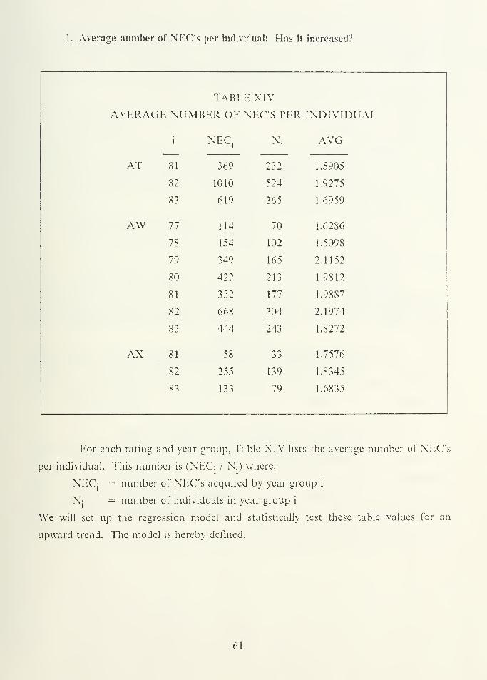
1. Average number of NEC's per individual: Has it increased?

TABLE XIV

AVERAGE NUMBER OF NEC'S PER INDIVIDUAL

AT

i

81

NECj Ni

AVG

369 232 1.5905

82 1010 524 1.9275

83 619 365 1.6959

AW 77 114 70 1.6286

78 154 102 1.5098

79 349 165 2.1152

80 422 213 1.9812

81 352 177 1.9887

82 668 304 2.1974

83 444 243 1.8272

AX 81 58 33 1.7576

82 255 139 1.8345

83 133 79 1.6835

For each rating and year group, Table XIV lists the average number of NEC's

per individual. This number is (NECj / N-) where:

NEC: = number of NEC's acquired by year group i

N: = number of individuals in year group i

We will set up the regression model and statistically test these table values for an

upward trend. The model is hereby defined.

61

77 78 79 80 81 82 S3

AW1

^

MODEL: Yj = pQ+ 0^ + £;

INDEX: i = year group

Y: = average number of NEC's per individual from year group i

P = constant number of NEC's per individual

p\ = change in Y per unit change in X (slope)

Xj = year group i

£• = error terms that are iid N(0, g )

The same methodology presented in the previous section will be used. The

F-test will determine if a trend exists and the one sided t-test will ascertain the direction

of the trend. The hypothesis tests and decision rules are presented in Tables XV and

XVI.

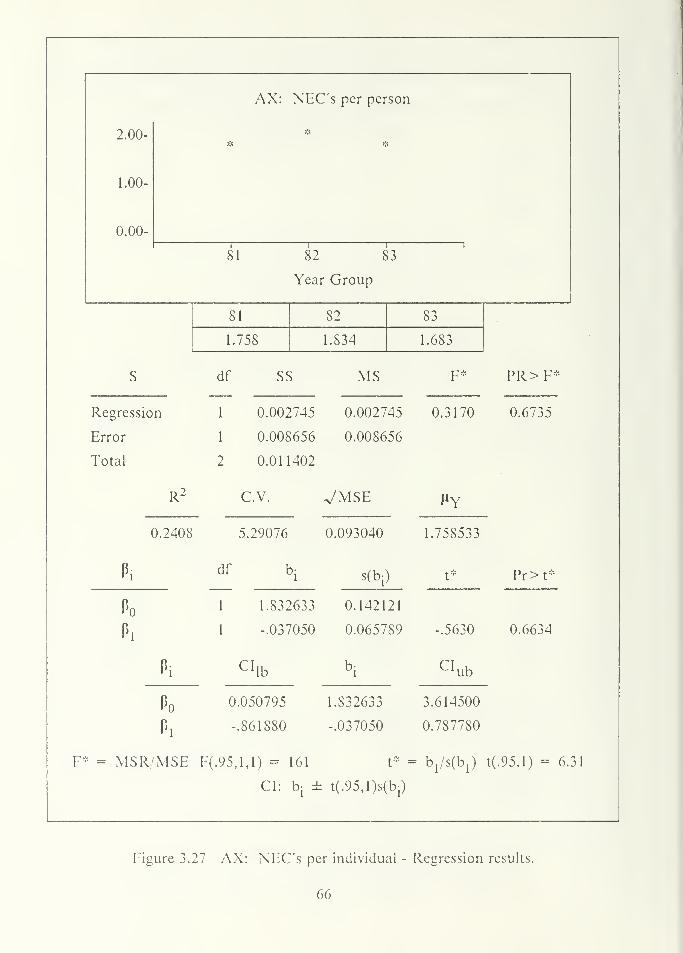
See Figures 3.25, 3.26, and 3.27. The test results clearly show that a trend is

absent. The F-test forces us to accept the null hypothesis in all three cases. Likewise,

the t-test directs us to accept the null hypothesis. We conclude this subsection by

saying: "The average number of NEC's per individual is not increasing."

2. Average number of NEC's per year group: Has it increased?

The first method for determining the amount of specialized training condensed

our data base into a few observations. We all know that a small sample size does not

provide a powerful statistical result. The second method uses the single factor

ANOVA model. We wanted to increase the number of observations in the test and use

a balanced design. We took a random sample of 30 data points from each year group

and tested the sample means for statistical differences. We present the model.

62

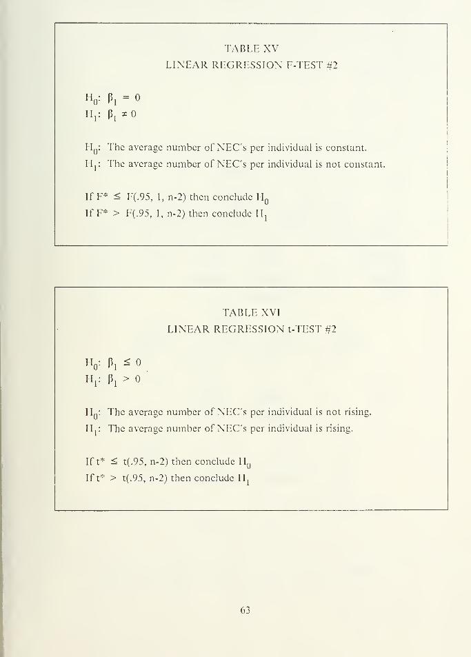
TABLE XV

LINEAR REGRESSION F-TEST #2

H : IV=

H r Pi *o

H : The average number of NEC's per individual is constant.

H r The average number of NEC's per individual is not constant.

IfF * < F(.95, 1 n-2) then conclude LL

If F * > F(.95, 1, n-2) then conclude H1

TABLE XVI

LINEAR REGRESSION t-TEST #2

H : P, <

FL: P, >

LL: The average number of NEC's per individual is not rising.

FL: The average number of NEC's per individual is rising.

If t* < t(.95, n-2) then conclude II

If t* > t(.95, n-2) then conclude ITj

63

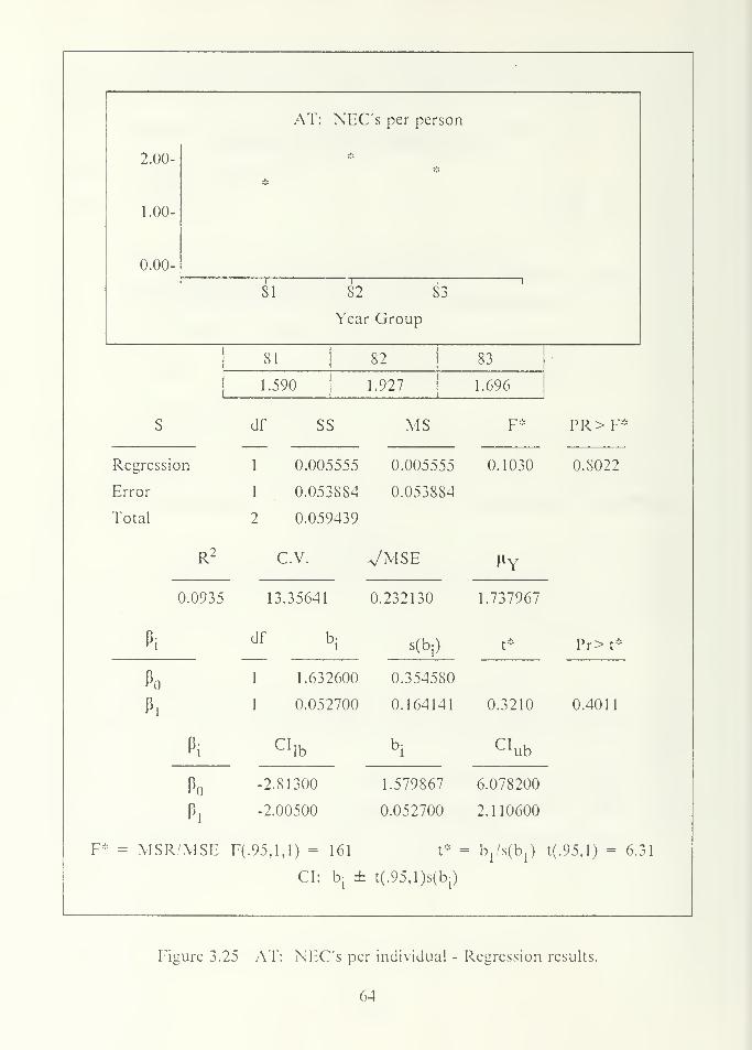
AT: NEC!'s per person

2.00- *y-

1.00-

0.00-

81 82 S3i

Yeai Group

81 82 83

1.590 1.927 1.696

s df SS MS F* PR>F*

Regrcssion 1 0.005555 0.005555 0.1030 0.8022

Error 1 0.053884 0.053SS4

Total 2 0.059439

(

R2 c.v. Vmse my

).0935 13.35641 0.232130 1.737967

Pi df bjs(bi)

0.354580

t* Pr>t*

Po 1 1.632600

Pi 1 0.052700 0.164141 0.3210 0.4011

h CIlb

bi

7

CI ub

Po -2.81300 1.57986 6.078200

Pi -2.00500 0.052700 2.110600

F* = MSR/MSE F(.95,l,l) = 161

CI: bj ±

t* _

t(.95,l)s(bi)

ty.sibj) t(.95.1) = 6.31

Figure 3.25 AT: NEC's per individual - Regression results.

64

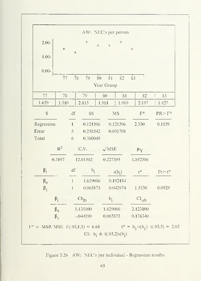
AW: NEC's per person

2.00- # A

*

1.00-

*

0.00-

77 78 79 80 81 82i i

S3

Year Group

77 78 79 so 81 82 83

1.629 1.510 2.115 1.981 1.989 2.197 1.S27

S df

1

SS MS F* PR>F*

Regression 0.121506 0.121506 2.350 0.1859

Error 5 0.258542 0.051708

Total 6 0.380048

R2 C.V. VMSE My

(3.3197 12.01502 0.227395 1.892586

Pidf

1

b! (bj)

721S4

t* Pr>t*

Pn 1.629086 0.1

pj 1 0.065875 0.042974 1.5330 0.0929

PiCI

lbb

i

CI ub

P 1.135100 1.629086 2.123100

p2

-.044590 0.065875 0.176340

F* = MSR/MSE F(.95,l,5) = 6.61 t* = b1/s(b

1) t(.95,5) = 2.02

CI: bj ± t(.95,2)s(bi)

Figure 3.26 AW: NEC's per individual - Regression results.

65

AX: NEC's per person

2.00-* *

1.00-

0.00-

81 82 83i

Year Group

81 82 83

1.758 1.834 1.683

s df SS MS F* PR>F*

Regression 1 0.002745 0.002745 0.3170 0.6735

Error 1 0.008656 0.008656

Total 2 0.011402

(

R2 c.v. Vmse my

3.2408 5.29076 0.093040 1.758533

p. df bjs(bj)

0.142121

t* Pr>t*

Po 1 1.832633

Pi 1 -.037050 0.065789 -.5630 0.6634

Pi CIlb

bi

CIub

h 0.050795 1.832633 3.614500

Pi -.861S80 -.037050 0.787780

F* = MSR, MSE F(.95,l,l) = 161

CI: b| ±

t* =

1095,1)8(1*,)

bj/sCbj) t(.95.1) = 6.31

Figure 3.27 AX: NEC's per individual - Regression results.

66

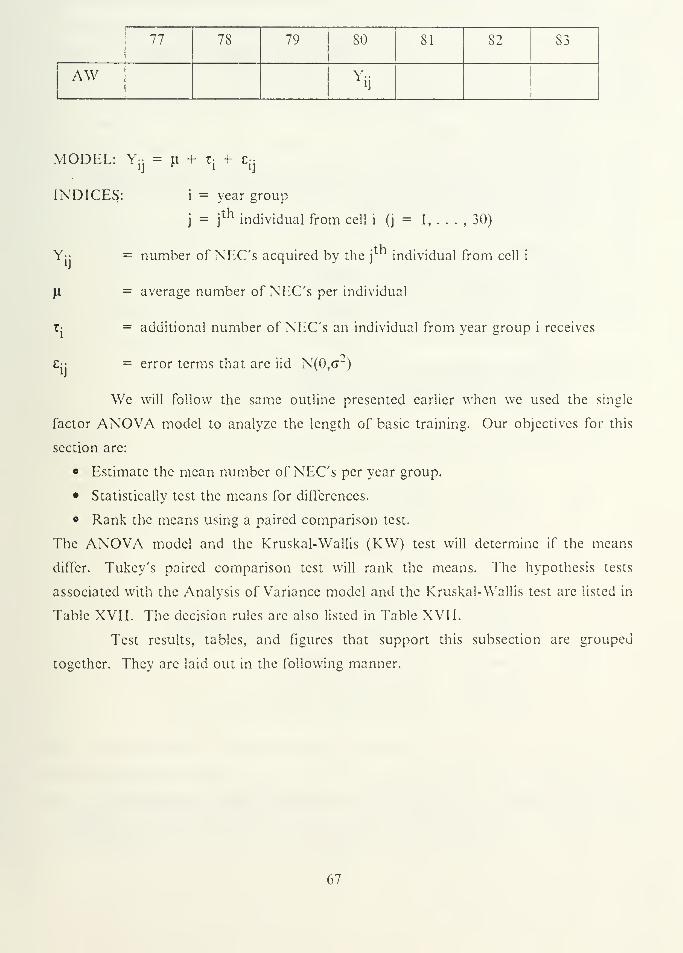
77 78 79 80 81 82 S3

AW Yii

MODEL: Y:ij

INDICES:

H + Z[+ €

i = year group

T;

j=

j individual from cell i (j= 1, . . . , 30)

= number of NEC's acquired by the j individual from cell i

= average number of NEC's per individual

= additional number of NEC's an individual from year group i receives

= error terms that are iid N(0,<T")

We will follow the same outline presented earlier when we used the single

factor ANOVA model to analyze the length of basic training. Our objectives for this

section are:

• Estimate the mean number of NEC's per year group.

• Statistically test the means for differences.

• Rank the means using a paired comparison test.

The ANOVA model and the Kruskal-Wallis (KW) test will determine if the means

differ. Tukey's paired comparison test will rank the means. The hypothesis tests

associated with the Analysis of Variance model and the Kruskal-Wallis test arc listed in

Table XVII. The decision rules are also listed in Table XVII.

Test results, tables, and figures that support this subsection are grouped

together. They are laid out in the following manner.

67

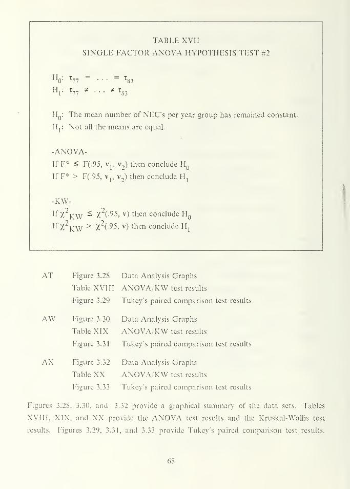
TABLE XVII

SINGLE FACTOR ANOVA HYPOTHESIS TEST #2

H : hi= T

83

Hr T77

* . .•

^ TS3

H : The mean number of NEC's per year group has remained constant.

«r Not all the means are equal.

-ANOVA-

If P < F(.95, Vj, v ) then conclude HQ

If P ' > F(.95, Vp v2) then conclude H,

-KW r

ur'KW < r(.95, V) then conclude HQ

\rr>

'KW > r'(.95, v) then conclude H,

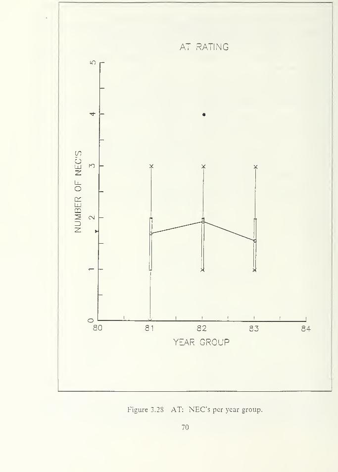
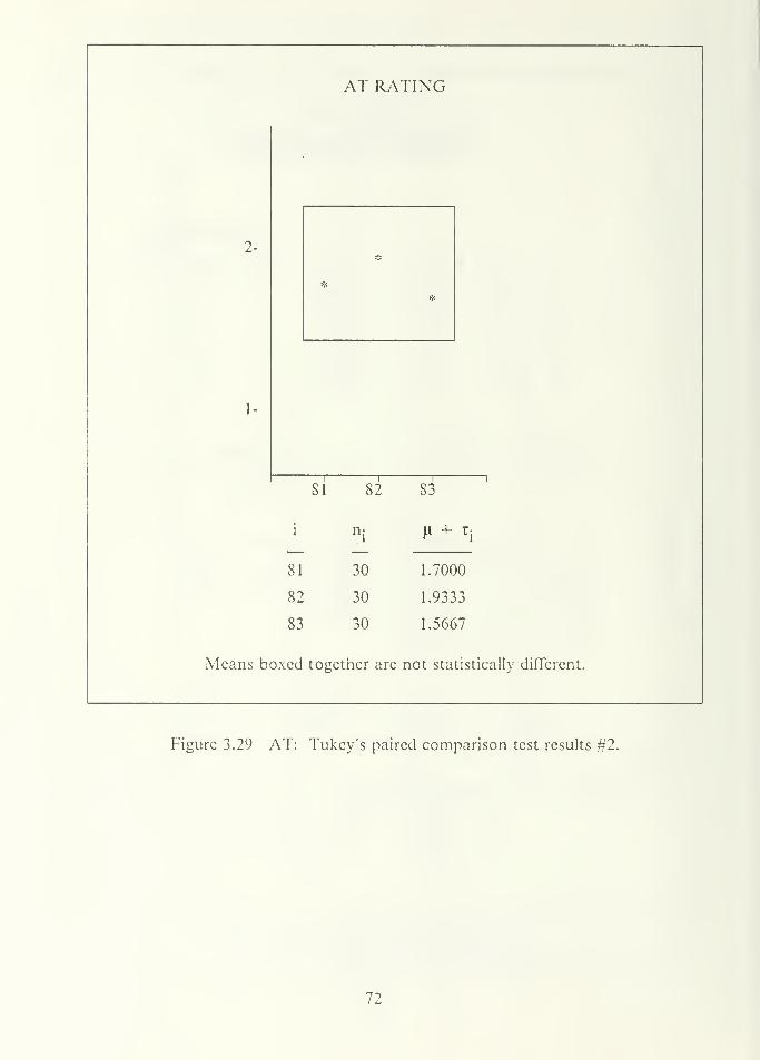
AT Figure 3.28 Data Analysis Graphs

Table XVIII ANOVA/KW test results


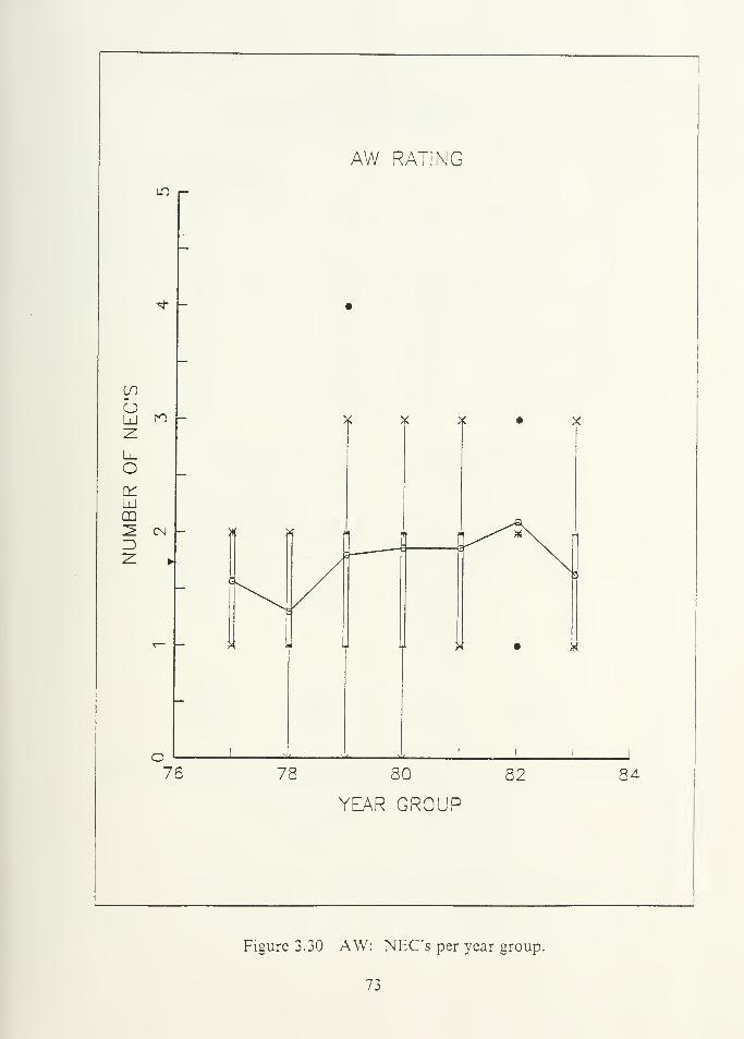
AW

AX

Figure 3.30

Table XIX

Figure 3.31

Figure 3.32

Table XX

Figure 3.33

Data Analysis Graphs

ANOVA, KW test results

Tukey's paired comparison test results

Data Analysis Graphs

ANOVA/KW test results

Tukey's paired comparison test results

Figures 3.28, 3.30, and 3.32 provide a graphical summary of the data sets. Tables

XVIII, XIX, and XX provide the ANOVA test results and the Kruskal-Wallis test

results. Figures 3.29, 3.31, and 3.33 provide Tukey's paired comparison test results.

68

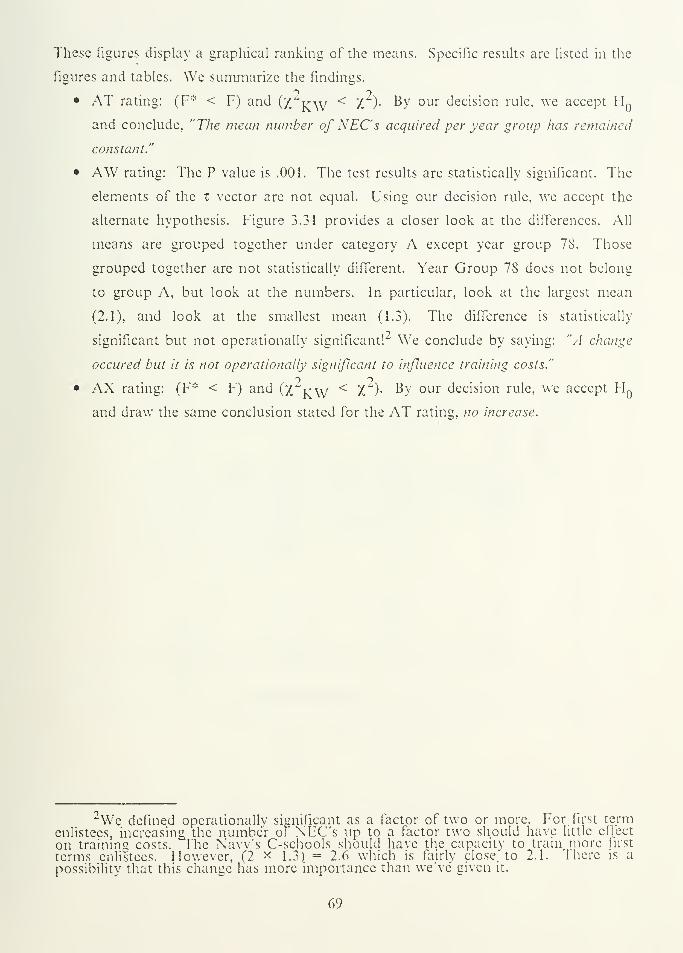
These figures display a graphical ranking of the means. Specific results arc listed in the

figures and tables. We summarize the findings.

• AT rating: (F* < F) and (X KW < a )• ^ our decision rule, we accept H

and conclude, "The mean number of NEC's acquired per year group has remained

constant."

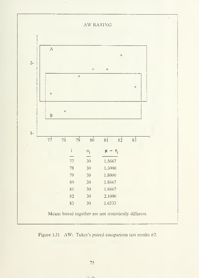
• AW rating: The P value is .001. The test results are statistically significant. The

elements of the z vector are not equal. Using our decision rule, we accept the

alternate hypothesis. Figure 3.31 provides a closer look at the differences. All

means are grouped together under category A except year group 78. Those

grouped together are not statistically different. Year Group 78 does not belong

to group A, but look at the numbers. In particular, look at the largest mean

(2.1), and look at the smallest mean (1.3). The difference is statistically

significant but not operationally significant!*" We conclude by saying: "A change

occured but it is not operationally significant to influence training costs."

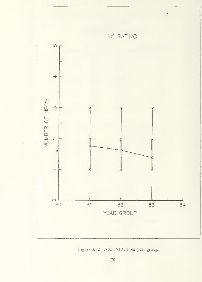
• AX rating: (F* < F) and (X KW < X ) By our decision rule, we accept H

and draw the same conclusion stated for the AT rating, no increase.

"We defined operationally significant as a factor of two or more. For. first termenlistees, increasing the number of NFC's up to a factor two should have little effect

on training costs. HThe Navy's C-schools should have the capacity to train, more first

terms enlistees. Flowever, (2 x 1.3) = 2.6 which is fairly close" to 2.1. I here is a

possibility that this change has more importance than we've given it.

69

LO

AT RATING

Id ro

O

LUCD

=3

80

M

81 82 83

YEAR GROUP

84

Figure 3.28 AT: NEC's per year group.

70

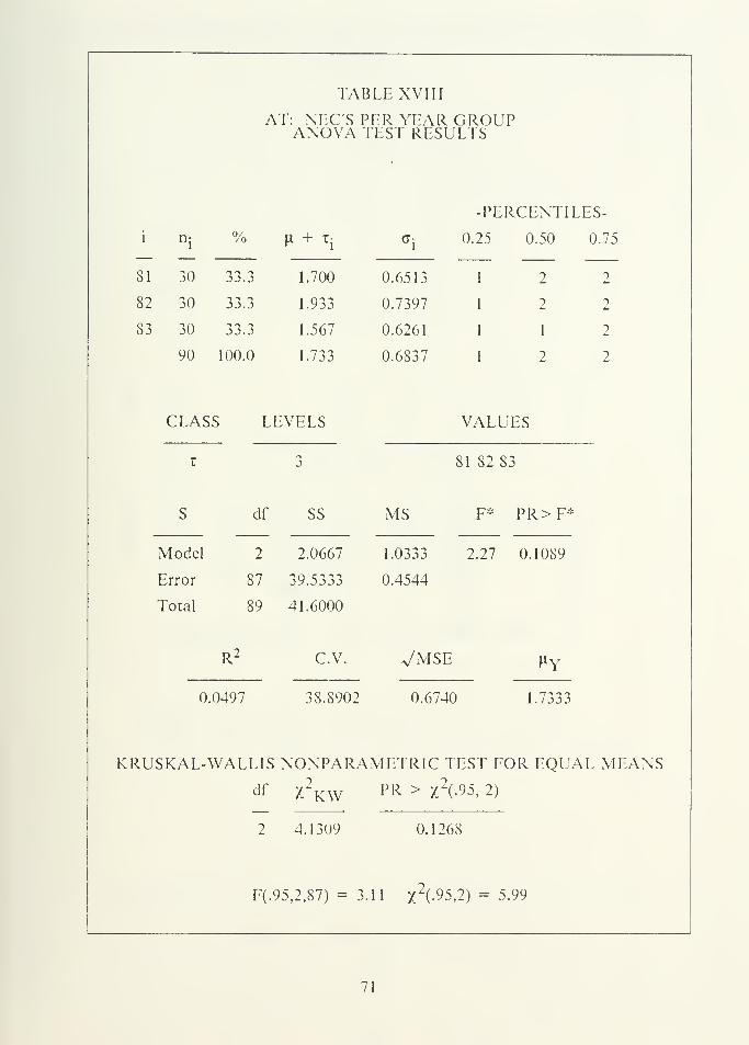
TABLE XVIII

AT: NEC'S PER YEAR GROUPANOVA TEST RESULTS

-PERCENTILES-

i nj % ]X + Ti

ffi

0.25 0.50 0.75

81 30 33.3 1.700 0.6513 1 2 2

82 30 33.3 1.933 0.7397 1 2 2

83 30 33.3 1.567 0.6261 1 1 2

90 100.0 1.733 0.6837 1 2 2

CLASS LEVELS VALUES

T 3 81 82 83

s df

2

SS MS F* PR>F*

Model 2.0667 1.0333 2.27 0.1089

Error 87 39.5333 0.4544

Total 89 41.6000

R2 c.v. Vmse HY

0.0497 38.8902 0.674C 1.7333

KRUSKAL-WALLIS NONPARAMETRIC TEST FOR EQUAL MEANSdf

2

2X KW PR > x

2(.95, 2)

4.1309 0.1268

F(- 95,2,87) = 3.11 x2(-95, 2) = 5.99

71

AT RATING

2-

1-

81 82 83

H + X:

81 30 1.7000

82 30 1.9333

83 30 1.5667

Means boxed together are not statistically different.

Figure 3.29 AT: Tukey's paired comparison test results #2.

LO t-

AW RATING

if)

Ld PO

O

1_U

2 c^

76

* H

¥ X x • x

M

78 SO

YEAR GROUP

82 84

Figure 3.30 AW: NEC's per year group.

73

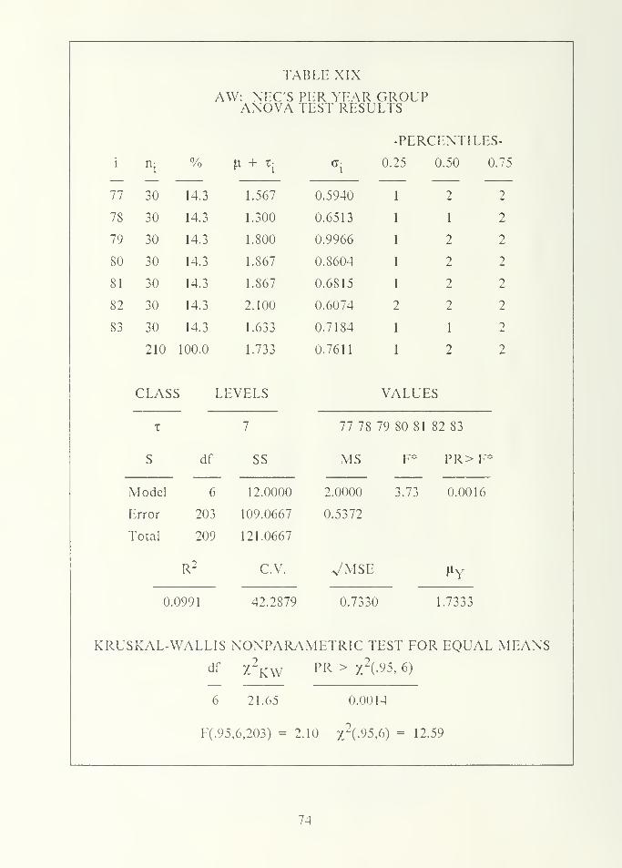
TABLE XIX

AW: NEC'S PER YEAR GROUPANOVA TEST RESULTS

-PERCENTILES-

i

77 30

%

14.3

\l + Tj (71

0.25 0.50 0.75

2 21.567 0.5940 1

78 30 14.3 1.300 0.6513 1 1 2

79 30 14.3 1.800 0.9966 1 2 2

80 30 14.3 1.867 0.8604 1 2 2

81 30 14.3 1.S67 0.6815 1 2 2

82 30 14.3 2.100 0.6074 2 2 2

83 30 14.3 1.633 0.7184 1 1 2

210 100.0 1.733 0.7611 1 2 2

CLASS LEVELS VALUES

t 7 77 78 79 SO 81 82 83

S df

6

SS MS F* PR>F*

Model 12.0000 2.0000 3.73 0.0016

Error 203 109.0667 0.5372

Total 209 121.0667

R2 c.v. VMSE HY

0.0991 42.2S79 0.7330 1.7333

KRUSKAL-WALLIS NONPARAMETRIC TEST FOR EQUAL MEANS

df

6

Y 2/ KW PR > x2(-95, 6)

21.65 0.0014

F(.95,6,203) = 2 10 r(.95,6) = 12. 59

74

2-

1-

AW RATING

A*

y-

*

B

?'.

i

77 78 79 80 81 82

i nj p + xl

i

83

Means

11 30 1.5667

78 30 1.3000

79 30 1.8000

SO 30 1.8667

81 30 1.S667

82 30 2.1000

83 30 1.6333

boxed together are not statistically different

Figure 3.31 AW: Tukcy's paired comparison test results #2.

75

•

AX RATING

lO

-* -

mLJ Ô

-z,

_ >i > (

^c

o

NUMBER 2 mm a •

Q

-

i |

:

i

'!

80 8 1 82

YEAR GROUP

8 3 84

Figure 3.32 AX: NEC's per year group.

76

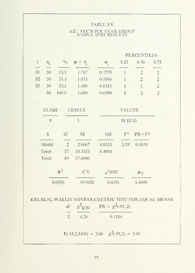
TABLE XXAX: NEC'S PER YEAR GROUP

ANOVA TEST RESULTS

-PERCENTILES-

i nj % H -I- tj Cj 0.25 0.50 0.75

81 30 33.3 1.767 0.7279 1 2 2

82 30 33.3 1.833 0.5560 1 2 2

83 30 33.3 1.400 0.6215 1 1 2

90 100.0 1.600 0.6500 1 2 2

CLASS LEVELS VALUES

T 3 81 82 83

s df

2

SS MS F* PR> F*

Model 2.0667 1.0333 2.53 0.0855

Error 87 35.5333 0.40S4

Total 89 37.6000

R2 c.v. VMSE HY

0.0550 39.9428 0.6391 1.6000

KRUSKAL-WALLIS NONPARAMETRIC TEST FOR EQUAL MEANSdf

2

V 2% KW PR > x

2(-95, 2)

4.26 0.1186

F(.95 ,2,H09) = 3.00 X2(.95,2) = 5.99

77

AX RATING

2-*

*

*

1-

81 82 83

i ni

H + x{

81 30 1.7667

82 30 1.6333

83 30 1.4000

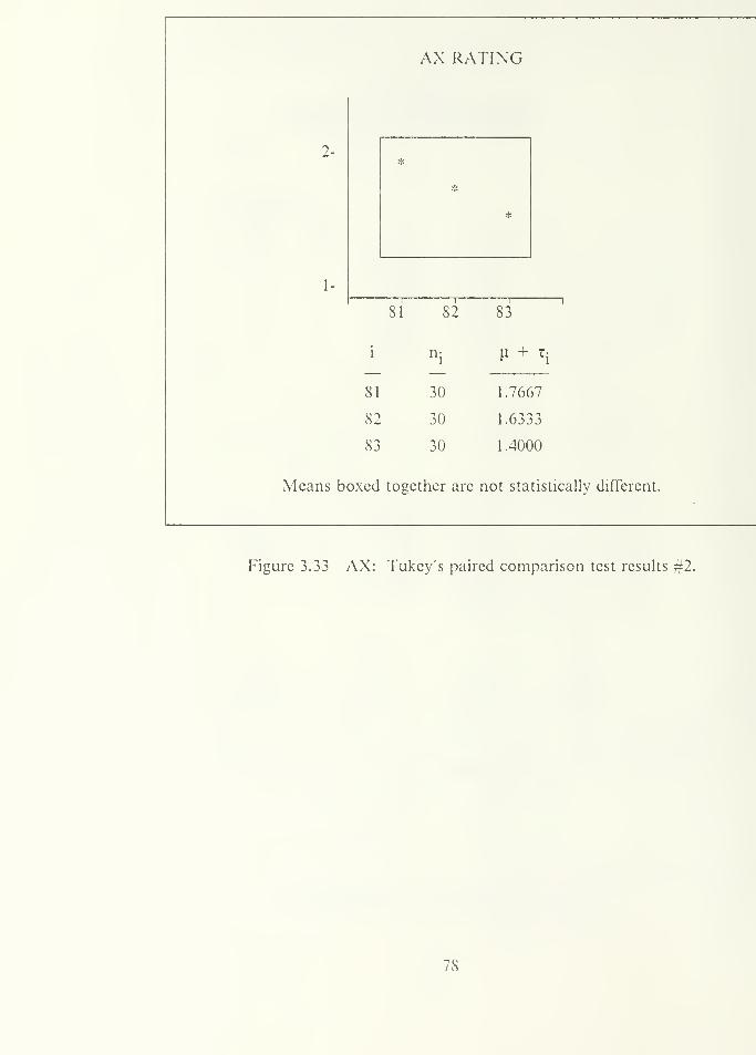
Means boxed tog ether are not statistically different.

Figure 3.33 AX: Tukey's paired comparison test results #2.

78

IV. MAIN RESULTS AND CONCLUSIONS

We started off with the following question, "What are the factors causing training

costs to rise?" To understand the problem, we formulated several reasons why we

think training costs are rising. Those reasons are:

• The length of basic training has increased.

• Attrition has increased.

• The amount of specialized training has increased.

We set out to verify those reasons using some historical data compiled by CNA.

The scope of this study is limited. The results are valid within the following

confines.

• Inferences are made with respect to these enlisted ratings, AT, AW, and AX.

• The expected career path is Boot Camp -» A-School -» Fleet. Inferences are

further restricted to those individuals that followed the expected career path.

• The overall time frame is restricted to the first enlistment period.

• The first 24 months is the time constraint for two areas of study, Basic Training

and Attrition.

• The second and third years of service is the time constraint for the last area of

study, Specialized Training.

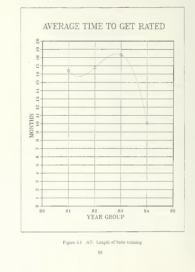
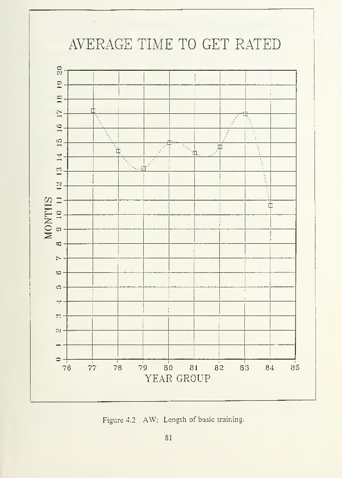
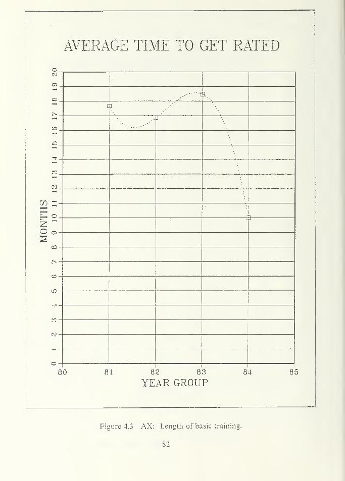
A. SUMMARY1. (Length of Basic Training — not a factor) The length of basic training has

cycled up and down. It has fluctuated over the years but there is no evidence

to suggest a steady increase over the years. Figures 4.1, 4.2, and 4.3 provide

graphical summaries. In all three cases, the final trend is encouraging, the

length of basic training has decreased.

2. (Attrition — not a factor) Losses in Basic Training are roughly constant from

year to year. Attrition has not increased.

3. (Amount of specialized training — not a factor) Specialized training has

remained constant. The amount has not increased.

79

o

AVERAGE TIME TO GET RATED

MONTHS

)

6

7

8

9

10

11

12

13

14

15

16

17

18

19

2

i

i

i

i

i

i

i

i

i

i

i

i

i

i

p i.

c — *

c ]

UJ

^

CO

tv

°i

80 81 82 83 84 8

YEAR GROUP5

Figure 4.1 AT: Length of basic training.

80


CM

oa-1

CO»H

i> [ ]

—

H

."' L J

COy—1

m t • -

c ]

J •,

: i. ..•

rH

CO ''•••E]'

1—

1

CO J»H

r/^ ^C]

2UU

CO

HJ

"T

CO

i-H —

o -1

76 77 78 79 80 81 82 83 84 85

YEAR GROUP

Figure 4.2 AW: Length of basic training.

81

o


MONTHS

[

56

7

8

9

10

11

12

13

14

15

16

17

18

19

2

i

i

i

i

i

i

i

i

i

i

i

i

i

i

i

...-—

E

1.

c 3

.1 J

riL{

"^T

tT J

uv

°i i 1

80 81 82 83 84 8

YEAR GROUP5

Figure 4.3 AX: Length of basic training.

82

B. RECOMMENDATIONSThis study looked at a small piece of the problem. The final result is that we

were unable to identify any factors causing training costs to rise. However, here is a

list of general questions that may be of interest for further research.

1. Has the length of basic training increased for enlisted ratings other than AT,

AW, and AX?

2. Has the amount of specialized training increased after the first enlistment

period?

3. Is the selection process effective?3

4. Has the Training Command's support costs increased?

5. Are training costs rising due to increased or improved training resources?

This list is by no means exhaustive. It is a few questions that we can ask. but were

unable to answer in this study.

The selection process is primarily based upon test scores and education level. If

the selection process is effective, then people screened for a particular rating will

complete that training prosram. The attrition rate will be low and survivability high.However, if we do not screen people properlv, the number of people that complete theprogram will be much less than optimal. Attrition will be high. The cilcct is highertraining costs. An elfectivc selection process produces savings.

83

APPENDIX A

MODEL ASSUMPTIONS

Throughout this study, we used two models extensively, the REGRESSION

model and the ANOVA model. Both models helped us to conceptualize the problem

and analyze the observations. The purpose of both models is to describe the events of

the past. These models are also used to predict and control events, but we're not

interested in using it for those matters.

In this appendix, we will briefly assess the aptness of the model. Is the model

appropriate for the data set at hand? This is an important question. It should be

answered whenever models are used. The importance of aptness is best described by

logic's implication statement, if P then Q, (P -» Q). If the model is appropriate, then

the ensuing analysis presented by the model is correct. Good analysis is conditioned

on the fact that the analyst use the appropriate models. The appropriateness of a

model is dependent upon adherence to the assumptions imbedded within the model.

We emphasized the importance of examining the aptness of a model, but how do

we confirm that a model is appropriate? Residual analysis is the tool for this task. It

is highly effective for spotting major departures from the assumed model. Our goal is

to verify the model assumptions by using residual analysis. In the statistical world, this

verification follows the mentality used in the U.S. court system, where we assume the

defendant to be innocent and prove beyond reason of doubt that the person is guilty.

In our profession, we assume the model assumptions arc correct and prove otherwise.

The major purpose of residual analysis is to detect serious departures from the

conditions assumed by the model.

Strict adherence to every assumption is not possible with this data set. A few

departures exist however, the departures are not substantial. Our first discussion

centers around the regression model. The second part deals with the ANOVA model.

Assumptions arc listed for each model. This is followed by a short summary discussing

the verification procedures and any effects caused by a departure from the model.

Figures and tables pertain to the AW rating. Similar results were obtained for the AT

and AX ratings.

S4

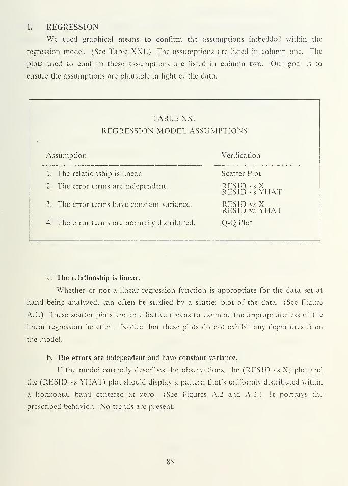
1. REGRESSION

We used graphical means to confirm the assumptions imbedded within the

regression model. (See Table XXI.) The assumptions are listed in column one. The

plots used to confirm these assumptions are listed in column two. Our goal is to

ensure the assumptions are plausible in light of the data.

Assumption

TABLE XXI

REGRESSION MODEL ASSUMPTIONS

Verification

1. The relationship is linear.

2. The error terms are independent.

3. The error terms have constant variance.

4. The error terms are normally distributed.

Scatter Plot

RES ID vs XRESID vs YMATRES ID vs XRESID vs YHAT

Q-Q Plot

a. The relationship is linear.

Whether or not a linear regression function is appropriate for the data set at

hand being analyzed, can often be studied by a scatter plot of the data. (See Figure

A.l.) These scatter plots are an effective means to examine the appropriateness of the

linear regression function. Notice that these plots do not exhibit any departures from

the model.

b. The errors are independent and have constant variance.

If the model correctly describes the observations, the (RESID vs X) plot and

the (RESID vs YHAT) plot should display a pattern that's uniformly distributed within

a horizontal band centered at zero. (See Figures A. 2 and A. 3.) It portrays the

prescribed behavior. No trends are present.

85

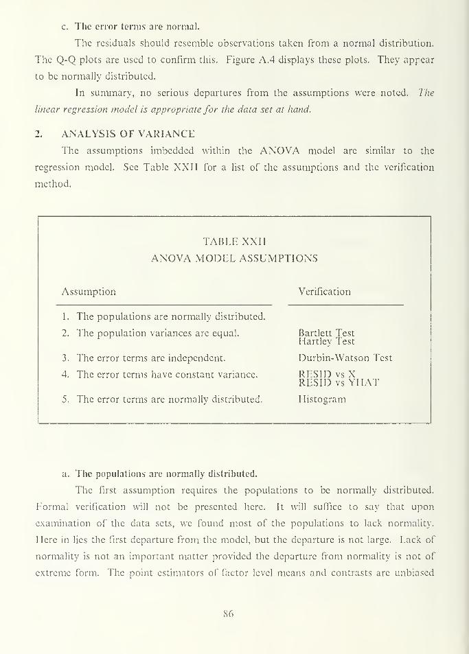
c. The error terms are normal.

The residuals should resemble observations taken from a normal distribution.

The Q-Q plots are used to confirm this. Figure A.4 displays these plots. They appear

to be normally distributed.

In summary, no serious departures from the assumptions were noted. The

linear regression model is appropriate for the data set at hand.

2. ANALYSIS OF VARIANCE

The assumptions imbedded within the ANOVA model are similar to the

regression model. See Table XXII for a list of the assumptions and the verification

method.

TABLE XXII

ANOVA MODEL ASSUMPTIONS

A.ssumption Verification

1. The populations are normally distributed.

2. The population variances arc equal. Bartlett TestHartley Test

3. The error terms are independent. Durbin-Watson Test

4. The error terms have constant variance. RESID vs XRES ID vs YHAT

5. The error terms are normally distributed. Histogram

a. The populations are normally distributed.

The first assumption requires the populations to be normally distributed.

Formal verification will not be presented here. It will suffice to say that upon

examination of the data sets, we found most of the populations to lack normality.

Here in lies the first departure from the model, but the departure is not large. Lack of

normality is not an important matter provided the departure from normality is not of

extreme form. The point estimators of factor level means and contrasts arc unbiased

86

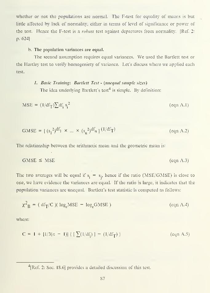
whether or not the populations are normal. The F-test for equality of means is but

little affected by lack of normality, either in terms of level of significance or power of"

the test. Hence the F-test is a robust test against departures from normality. [Ref. 2:

p. 624]

b. The population variances are equal.

The second assumption requires equal variances. We used the Bartlett test or

the Hartley test to verify homogeniety of variance. Let's discuss where we applied each

test.

/. Basic Training: Bartlett Test - {unequal sample sizes)

The idea underlying Bartlett's test4

is simple. By definition:

MSE = (l/dfT)£df Sj2 (cqn A.l)

GMSE = [(Sj2)^ x ... x (s

n2)dfn ]

O/dfj) (eqnA.2)

The relationship between the arithmetic mean and the geometric mean is:

GMSE < MSE (eqn A. 3)

The two averages will be equal if s;

= s- hence if the ratio (MSE/GMSE) is close to

one, we have evidence the variances are equal. If the ratio is large, it indicates that the

population variances are unequal. Bartlett's test statistic is computed as follows:

X2B- ( dfT/C )( log

eMSE - log

eGMSE ) (cqn A.4)

where:

C = 1 + [l/3(n -1)] { [

V(i/d f.) ]- (l/dfT) } (cqn A.5)

[Ref. 2: Sec. 18.6] provides a detailed discussion of this test.

87

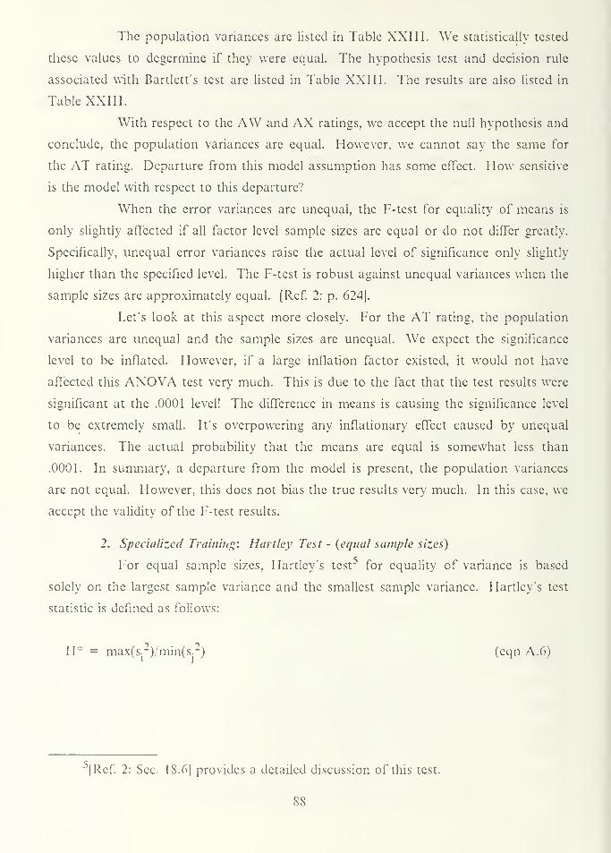
The population variances are listed in Table XXIII. We statistically tested

these values to dcgcrminc if they were equal. The hypothesis test and decision rule

associated with Bartlett's test arc listed in Table XXIII. The results are also listed in

Table XXIII.

With respect to the AW and AX ratings, we accept the null hypothesis and

conclude, the population variances are equal. However, we cannot say the same for

the AT rating. Departure from this model assumption has some effect. How sensitive

is the model with respect to this departure?

When the error variances are unequal, the F-test for equality of means is

only slightly affected if all factor level sample sizes are equal or do not differ greatly.

Specifically, unequal error variances raise the actual level of significance only slightly

higher than the specified level. The F-test is robust against unequal variances when the

sample sizes are approximately equal. [Ref. 2: p. 624].

Let's look at this aspect more closely. For the AT rating, the population

variances are unequal and the sample sizes are unequal. We expect the significance

level to be inflated. However, if a large inflation factor existed, it would not have

affected this ANOVA test very much. This is due to the fact that the test results were

significant at the .0001 level! The difference in means is causing the significance level

to be extremely small. It's overpowering any inflationary effect caused by unequal

variances. The actual probability that the means are equal is somewhat less than

.0001. In summary, a departure from the model is present, the population variances

are not equal. However, this does not bias the true results very much. In this case, we

accept the validity of the F-test results.

2. Specialized Training: Hartley Test - (equal sample sizes)

For equal sample sizes, Hartley's test for equality of variance is based

solely on the largest sample variance and the smallest sample variance. Hartley's test

statistic is defined as follows:

II* = max(s. 2)/min(s.

2) (eqn A. 6)

[Ref. 2: Sec. 18.6] provides a detailed discussion of this test.

8S

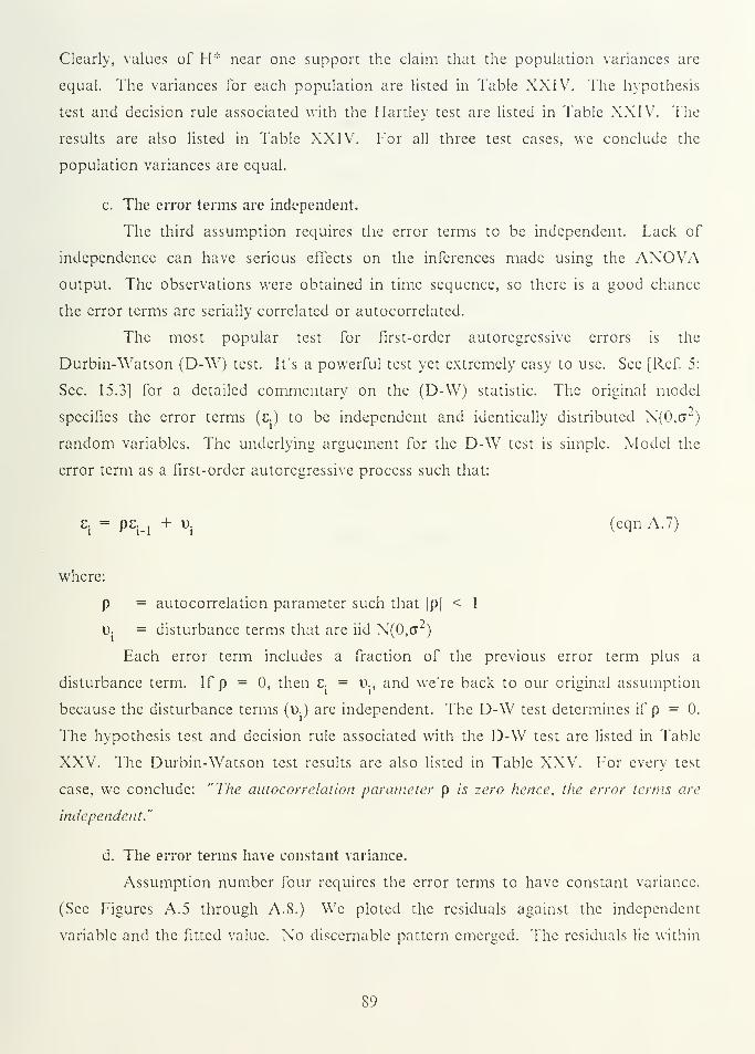
Clearly, values of H* near one support the claim that the population variances are

equal. The variances for each population are listed in Table XXIV. The hypothesis

test and decision rule associated with the Hartley test are listed in Table XXIV. The

results are also listed in Table XXIV. For all three test cases, we conclude the

population variances are equal.

c. The error terms are independent.

The third assumption requires the error terms to be independent. Lack of

independence can have serious effects on the inferences made using the AXOVAoutput. The observations were obtained in time sequence, so there is a good chance

the error terms are serially correlated or autocorrelated.

The most popular test for first-order autoregressive errors is the

Durbin-Watson (D-W) test. It's a powerful test yet extremely easy to use. See [Ref. 5:

Sec. 15.3] for a detailed commentary on the (D-W) statistic. The original model

specifies the error terms (£.) to be independent and identically distributed N(0,ff )

random variables. The underlying arguement for the D-W test is simple. Model the

error term as a first-order autoregressive process such that:

£j = p£M 4- u. (eqn A. 7)

where:

p = autocorrelation parameter such that |p| < 1

l). = disturbance terms that are iid N(0,<T2)

Each error term includes a fraction of the previous error term plus a

disturbance term. If p = 0, then E. = u., and we're back to our original assumption

because the disturbance terms (o.) are independent. The D-W test determines if p = 0.

The hypothesis test and decision rule associated with the D-W test are listed in Table

XXV. The Durbin-Watson test results arc also listed in Table XXV. For every test

case, we conclude: "The autocorrelation parameter p is zero hence, the error terms are

independent."

d. The error terms have constant variance.

Assumption number four requires the error terms to have constant variance.

(See Figures A. 5 through A. 8.) We plotcd the residuals against the independent

variable and the fitted value. No discernable pattern emerged. The residuals lie within

89

a horizontal band centered at zero. Notice how the variance stays constant through

changes on the X-axis. This behavior is the expected behavior given the assumption is

correct. These plots give us no reason to reject the fourth assumption.

e. The error terms are normally distributed.

The last assumption requires the error terms to be normally distributed. We

plotted the residuals in the form of a histogram. (See Figures A. 9 and A. 10.) Both

plots resemble a normal distribution with mean zero. These plots verify the last

assumption.

In summary, the assumptions are reasonable. We have no reason to reject

them as incorrect. There is a few minor departures from the model, but due to the

robustness of the F-test, these departures did not affect the final results. We conclude:

The ANOVA model is appropriate for the data set at hand.

90

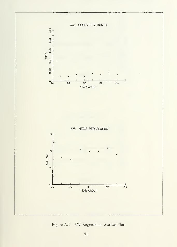
AW: LOSSES PER MONTHo

d

IBa

76 78 80 82 84

YEAR GROUP

AW: NEC'S PER PERSON

u

£

J [ I 1' '

76 78 80 82 84-

YEAR GROUP

Figure A. 1 AW Regression: Scatter Plot.

91

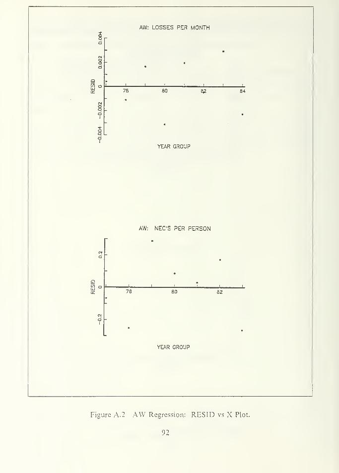
8d

AW: LOSSES PER MONTH

•

ood

••

QCO oLJa:

|i

78 80 8,2 84

sd

I

-

*

•

ood

•

YEAR GROUP


-•

d•

•

o00 !

•

78 80 82P

dI

••

YEAR GROUP

Figure A.2 AW Regression: RES ID vs X Plot.

92

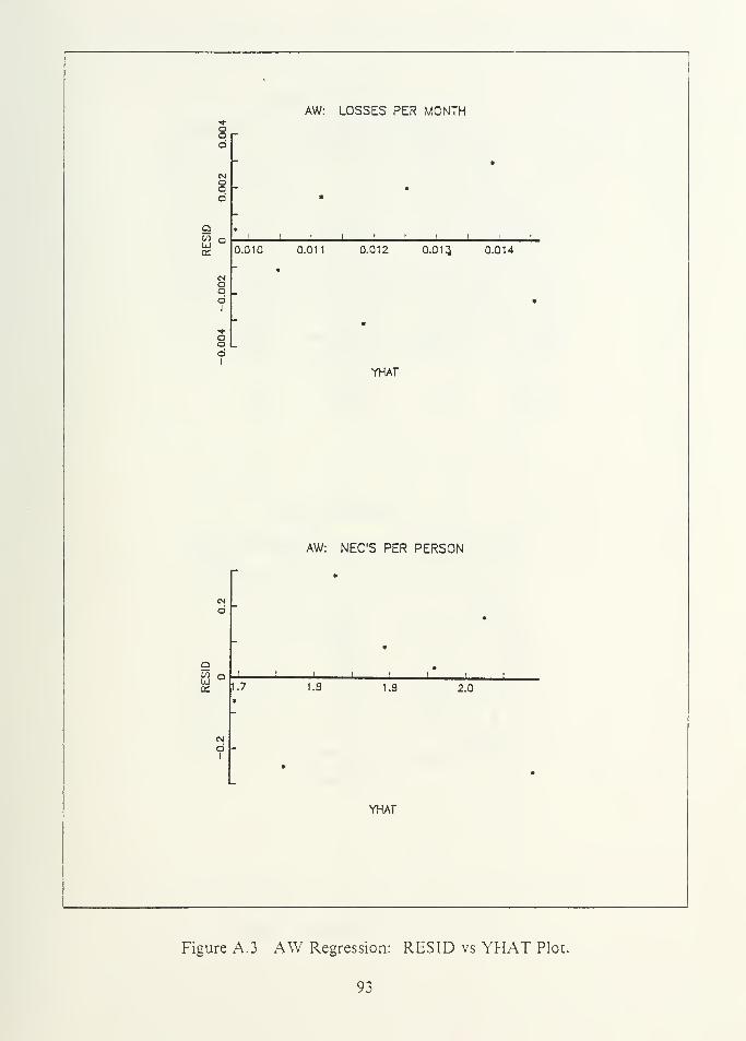
aod

AW: LOSSES PER MONTH

-•

ooa

- •*

au

•

l

i i i ii i i

I

0.010 0.011 0.012 0.013 0.014

oaa

l

«

*

aad

•

YHAT


•

d•

•

aCO oUJ

_l 1

*

1.7

•

1.8 1.9 2.0

dI

•*

YHAT

Figure A.3 AW Regression: RESID vs YHAT Plot.

93

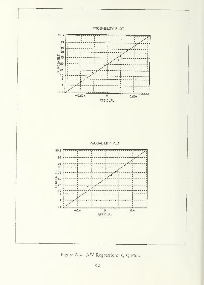
PROBABILITY PLOT

99.9

99

95

90ui=_75i—

5 5

cc

Ql

10

5

1

0.1

99.9

99

95

90UJ=.75i—

5so

UJ25

10

5

1

0.1

11

1 i jiii y'iii y^f \

L- I -! J-^-J1 i i i i/^

I -- L L L-Â J

I L L |_ _U2_._,J '

• I •I I

yS'iii y\r r

r -I—-rî ,'

î i i / *

i

i i i y>

j. r..™kf.„.

1_, j

[

"j" ;p^-i-~—

!

-i i

'

|L

~:z_j i"—

"i i i

S* I I I

J^-J- 1•- -"- -i -

-0.004

-0.4

RESIDUAL

PROBABILITY PLOT

0.004

u. i i i i i -ji I I i I I yS\I I I I I I y I

I I I I I I s I

» — — — — — — -i — — — — — — —i — — __*___ — — — - h- — — — — — — t-y- — - — — ti i i i i jr i

i i i i i >î i

I ______ -I ______ _l_ ______________ l_ _ _ -X- _-______!I I I I I >V^ I____________________ __ h.______ (

.—<£____ ^______ ti i i i jr i itiit >» ' ' '_________________________— -jS-*-r------r-- _— — — ti i i i ^^ I I i

i i i i >^ I I i

*______ _i — ___(-_— _- 4^» _- ———>-___-_ — »__ — — — _ +i i i >î i I i

I I I y* I I I I

1 J I__V1 I __l I 11 I • \/ I I I I

I I sT I I I I

I ______ -I — _ -X^- U---___U — __ — — -k — _ — —__4I I y4 I I I I I____________ ._,___ __t- ____,._- —_--,.-----_ -

I lyS I I I I I

I J^ I I I I I

1 _ - _ _ —_fj !_____ _.-__-_-_. —-_- —------ XP y I I I I I I

I / I I I I I I

I >/^ I I I I I I^'

I

*

0.4

RESIDUAL

Figure A.4 AW Regression: Q-Q Plot.

94

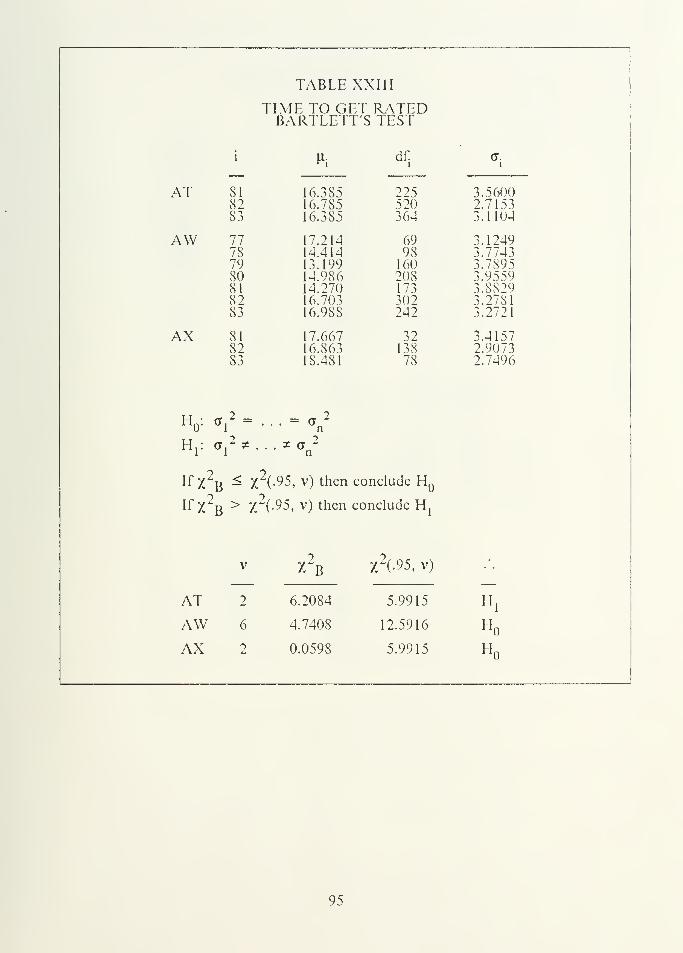
TABLE XXIII

TIME TO GET RATEDBARTLETT'S TEST

AT 818283

AW 77787980818283

AX 818283

H n : a.2 = . . .

= a :

1 n

H.: a,2 * . . . * <7

2

1 1 n

If x2g ^ X


Q

If X r > Z (-95, v) then conclude Hj

îdf.

i l

16.385 225 3.560016.785 520 2.715316.385 364 3.1104

17.214 69 3.124914.414 98 3.774313.199 160 3.789514.986 208 3.955914.270 173 3.882916.703 302 3.278116.988 242 3.2721

17.667 32 3.415716.S63 138 2.90731S.481 78 2.7496

V

2

X b X2(.95, v) •'•

AT 6.2084 5.9915 "i

AW 6 4.7408 12.5916 «oAX 2 0.0598 5.9915 H

o

95

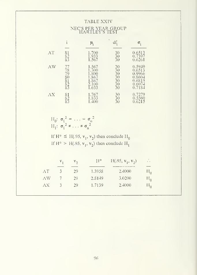
TABLE XXIV

NEC'S PER YEAR GROUPHARTLEY'S TEST

AT

AW

AX

H : ffj

H r a,

i * (If.i

30

a.i

81 1.700 0.651382 1.933 30 0.739783 1.567 30 0.6261

77 1.567 30 0.594078 1.300 30 0.651379 1.800 30 0.996680 1.867 30 0.860481 1.867 30 0.681582 2.100 30 0.607483 1.633 30 0.71S4

81 1.767 30 0.727982 1.833 30 0.556083 1.400 30 0.6215

2 _ 2. .

= <7"

n

2 *.n

If H* < H(.95, Vj, v2) then conclude H

Q

If H* > H(.95, Vj, v2) then conclude Hj

vl

3

v2

29

II* H(.95, v p v2 )

AT 1.3958 2.4000 I!

AW 7 29 2.8149 3.0200 «o

AX 3 29 1.7139 2.4000 H

96

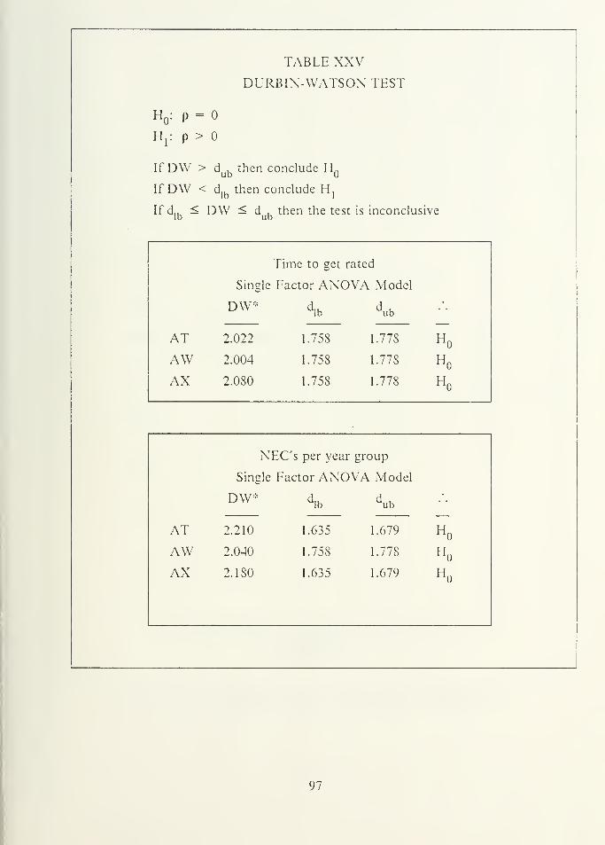
TABLE XXVDURBIN-WATSON TEST

H : p =

H,: p>0

IfDW > d , then conclude H nub

IfDW < d,bthen conclude Hj

If d. ^ DW — d . then the test is inconclusive

Time to get rated

Single Factor ANOVA Model

AT

DW* dlb ub

Ho

2.022 1.758 1.778

AW 2.004 1.758 1.778 Ho

AX 2.0S0 1.758 1.778 Ho

NEC's per year group


DW* d.lb ub

AT 2.210 1.635 1.679 H

AW 2.040 1.758 1.778 Ho

AX 2.180 1.635 1.679 Ho

97

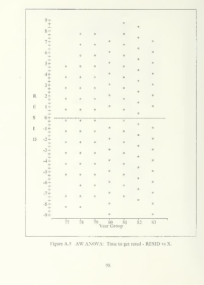
9 +4- *

4- *

8 +4-

*v * *

4-<•

74- * >'?

4- * J; *

+ *

6 + A *

4- * * #

4- *

5 + * *fc

+ & * *

4- *

4 + * *

4- * * * *

4-J;

34-J- *

4- * •jt* * *

4- *

R 2 + -'• *

4- * £ # *

4- &

E 1 + & .-:-.

4- * # J; *

4- *

S +_i_ *

4-/-

I -i + * :'i

+ * -i* ft *

+ *

D -24- * r'c

+ •h & * *

+ i*i

-3 + * *

4- & i' a *

4- *

-4 + * ?':

4-.-:-. 7''. * *

4- *

-5 + ;•- #

4- * * & •*

4- *

-6 + j»; *

4- * * *

4- *

-74- * ?*:

4-*» * * *

4- y*

-84- * *

4- * *

4-

-9 + * •

1 i

77 78 79 801

811

821 1

83Year G roup

Figure A. 5 AW ANOVA: Time to ect rated - RES ID vs X.

98

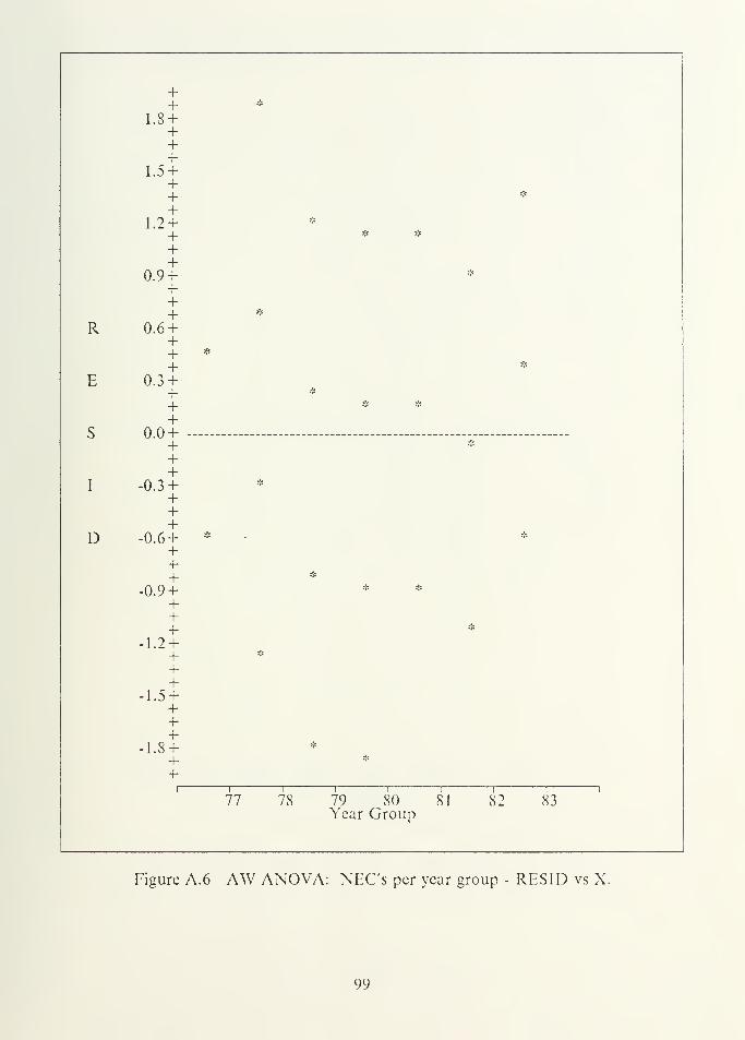
Figure A. 6 AW ANOVA: NEC's per year group - RESID vs X.

99

++

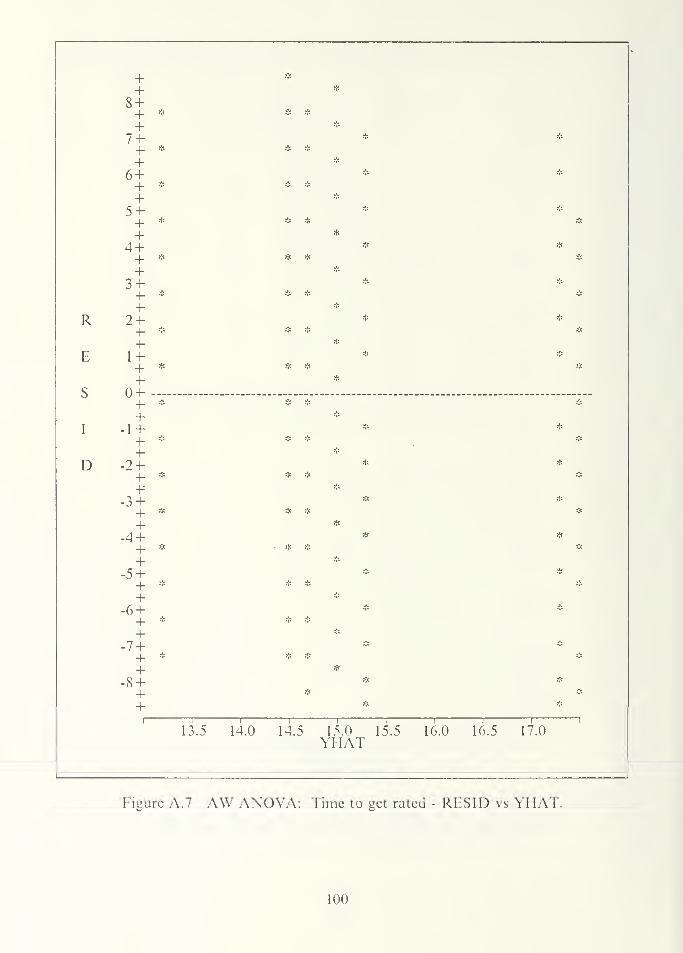
8 +++

7 +++

6 +++

5 +++

4 +++

3 +++

R 2 +

+S +

++

I -1 +++

D -2 ++ *

+-3 ++ *

+-4 ++ *

+-5 ++ *

+-6 ++ *

+-7 ++ *

+-8 +++

*+ *

+1 +

*

*

*

*

*

*

**

13.5 14.0 14.5 15.0 15.5 16.0 16.5 17.0YIIAT

~i

Figure A.7 AW ANOVA: Time to get rated - RES ID vs YHAT.

100

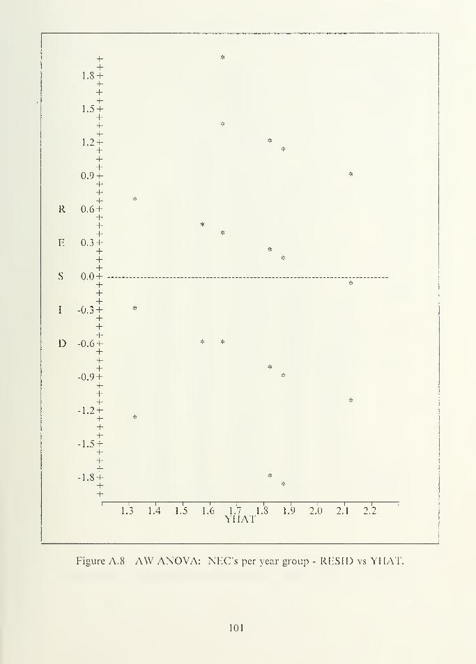
+1.8 +

+++

1.5 ++++

1.2 ++++

0.9 ++++

R 0.6 ++++

E 0.3 ++++

S 0.0 ++++

I -0.3 ++++

D -0.6 ++++

-0.9 +-f

++

-1.2 ++++

-1.5 +++-i-

-1.8 ++

*

*

i i i i i i i i i i i

1.3 1.4 1.5 1.6 1.7 1.8 1.9 2.0 2.1 2.2YIIAT

Figure A.8 AW ANOVA: NEC's per year group - RESID vs YIIAT.

101

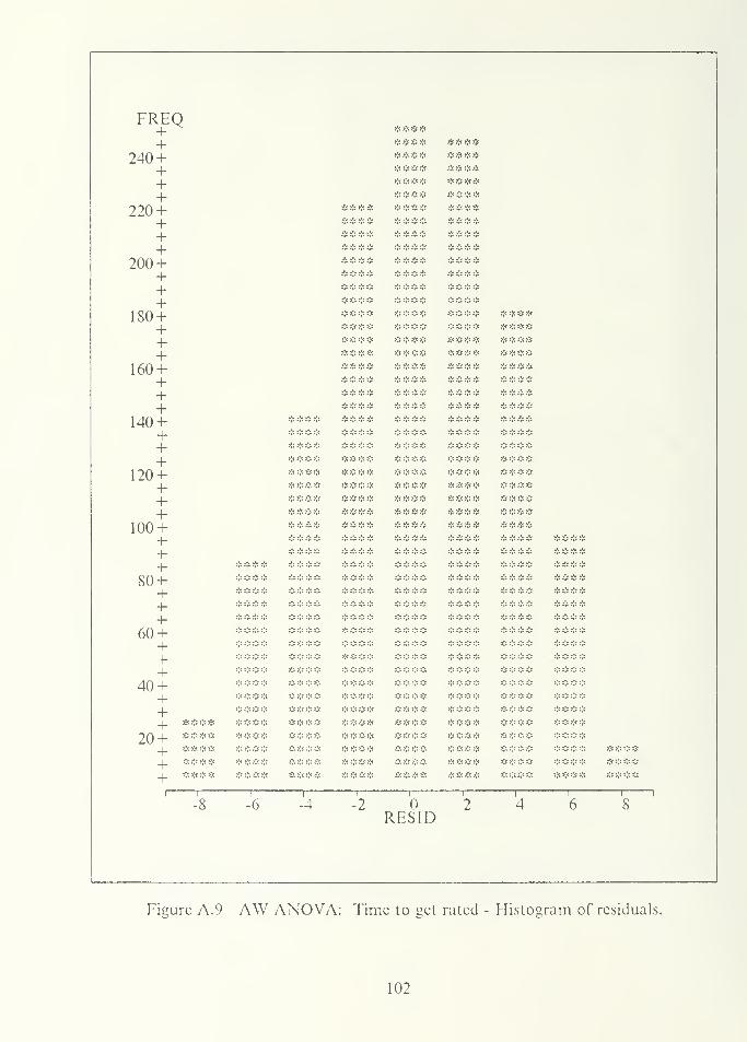
FREQ++

240 ++++

220 ++++

200 ++++

180 ++++

160 ++++

140 ++++

120 +++

100 ++++

80 ++++

60 ++

+40 ++++ •

20+ *

+ *

+ *

+ ::

i r

A .•- J- *>•. .'. .'. .'.

*r» -•, %•• «b

* * * * * * * * -:-. * -:-• ** * * * j, a *•„ j.

* * * : **** ?.-. ••:-. ••:= *

j- .•- .; .:

* * * * * * * * *****#$* ***** * * * **** >», .'. •£• J,

*#** :)- * $ * **** -it .-:-. ;;= .-:-

* # $ * **** ***>s * * # *$ * :•-•

.-I:

»•. .*, >'. „'. j. j» gtm ~f. ?;:

^-. :•: ;;:

* .-•: * * J- .», .*, -*. * .-;: :: .-•; :•: .-:: ;': .;:

* * * * * * ** * ::= •: *

**** * s * * A »•- .'. .A.

* * * * **** * •-:; * *

* * : * :;: * * :|: * ::•. ;|: *:.: .-;•. * .;:

.•„ .'. -J. .•» * * * * * * * *./. J- »*. -J. tfe o- „•. ..», *'. .'- *, J. * * * * * :.: * *

**** * .-•-. .-;-. * J. .•. .•. „•..-•.: * * .-;:

* * * * ;:=*:;: ::

: :.: * * * * * -•;•. * * *

*#*# * :I: :.

-

:

*

:;: :;: :\: :\: ***** ;:• * * *l( .b J« J- # * •!: -I:

J. *«, J. J. * * * ] :; * : :•.: 4> >•> ^« »•* ****J. ,•- ,'- J. * * * *

,'. .•- -». J- **** **** **** **** ***** .-:= * # * * * =:-. * * * * * ::-. .;-. .-:-. .-;: :;: :;: * ::; * •: :;

* :): .-•-. :". : * * :. :•: :•-. .-•-. .-): * * :-. .-;: * * :': * * * * * :;::;:::::::

« :.: « « * * :•: * * .-•: ;•-.

*

* :•: :;:

*

J, J. .** J. * ::- ^: *: :; * : : : * * * .;: ::: * **** * * * *

::-. « * :. -: * * * •-:•• .-:-• * * :;; * * * * * * * a. .•, .-. .- * * * *

***« **** .». .. .'. ^'. ****•^ ::-. .-:-. .•:--

... , ... ...

.', J- ^. -•*

* * *

*

* * * * * * * * * $ •:: * * ^ * ** .-:- * * * * * * :[: :;: :-. * * :\: :\: :\: * * * * * -:- * *j. .: .: .:

**** :--•::•: ****- -•-

... ... ... ... ^ ..- ..

-8 -6 -4 -2

RliSID

Figure A. 9 AW ANOVA: Time to get rated - Histogram of residuals.

102

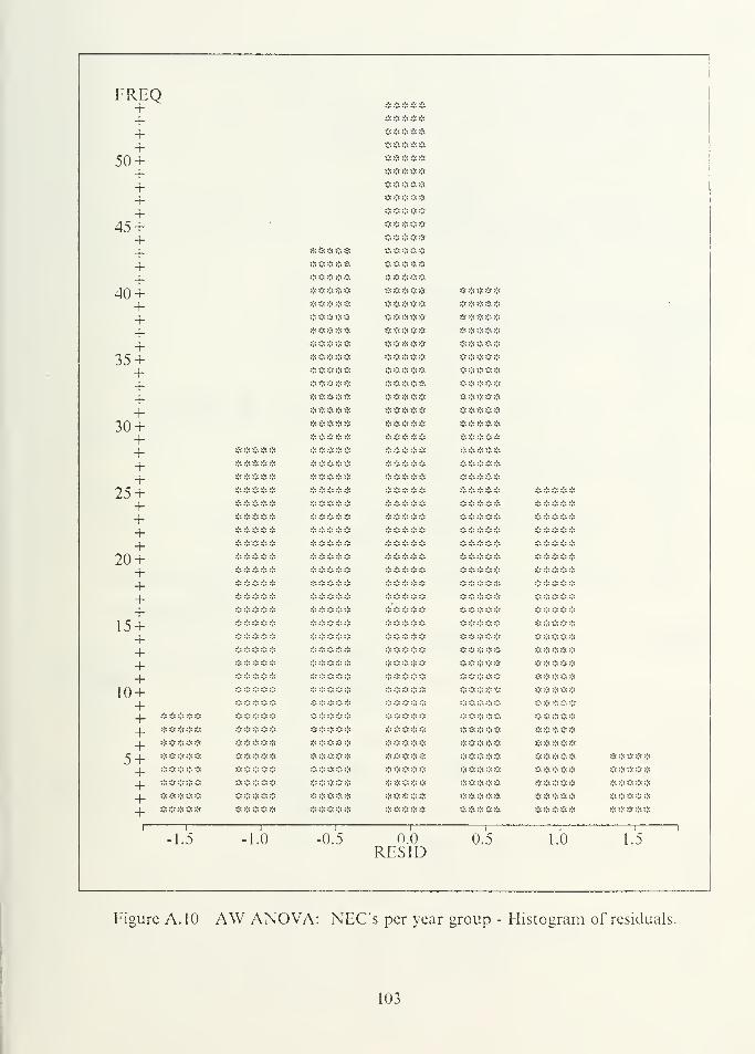
FREQ

+++

50 +++++

45 +++++

40 +++++

35 +++++

30 +++++

25 +++++

20 +++++

15 +++++

10 +++ *****+ *****

5+ *****+ *****+ *****+ *****

~r

* * * * * * : *

, *•- j.

... .'. ,•- .; .-

t-

1.5 -1.0 -0.5 0.0 0.5 1.0 1.5

RESID

Figure A. 10 AW ANOVA: NEC's per year group - Histogram of residuals.

103

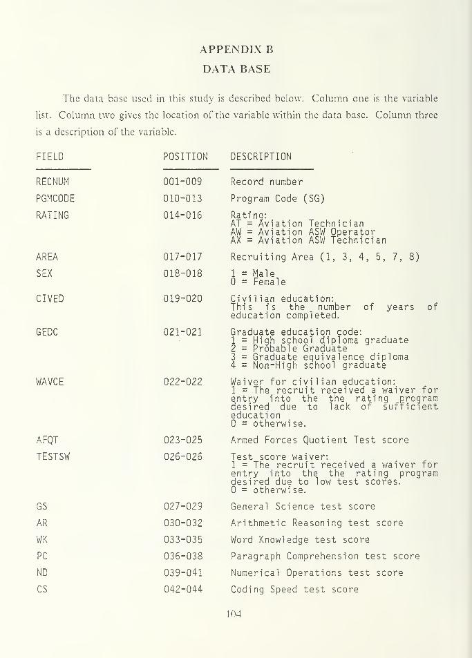
APPENDIX B

DATA BASE

The data base used in this study is described below. Column one is the variable

list. Column two gives the location of the variable within the data base. Column three

is a description of the variable.

FIELD POSITION DESCRIPTION

RECNUM 001-009 Record number

PGMCODE 010-013 Program Code (SG)

RATING 014-016 Rating:AT = Aviation TechnicianAW = Aviation ASW OperatorAX = Aviation ASW Technician

AREA 017-017 Recruiting Area (1, 3, 4, 5, 7, 8)

SEX 018-018 1 = Male= Female

CIVED 019-020 Civilian education:This is the number of years ofeducation completed.

GEDC 021-021 Graduate education code:1 = High school diploma graduate2 = Probable Graduate3 = Graduate equivalence diploma4 = Non-High school graduate

WAVCE 022-022 Waiver for civilian education:1 = The recruit received a waiver forentry into the the rating programdesired due to lack of sufficienteducation

= otherwise.

AFQT 023-025 Armed Forces Quotient Test score

TESTSW 026-026 Test score waiver:1 = The recruit received a waiver forentry into the the rating programdesired due to low test scores.

= otherwi se.

GS 027-029 General Science test score

AR 030-032 Arithmetic Reasoning test score

WK 033-035 Word Knowledge test score

PC 036-038 Paragraph Comprehension test score

ND 039-041 Numerical Operations test score

CS 042-044 Coding Speed test score

104

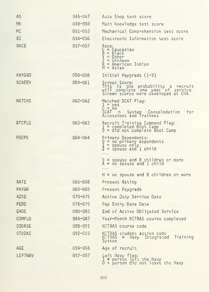
AS

MK

MC

EI

RACE

PAYGRD

SCREEN

MATCHS

RTCFLG

PDEPS

RATE

PAYGR

ADSD

PEBD

EAOS

COMPLD

COURSE

STUDAC

AGE

LEFTNAV

045-047 Auto Shop test score

048-050 Math Knowledge test score

051-053 Mechanical Comprehension test score

054-056 Electronic Information test score

057-057 Race:C = CaucasianB = BlackX = OtherZ = UnknownR = American IndianM = Asian

058-058 Initial Paygrade (1-9)

059-061 Screen Score:This is the probability a recruitwill complete one year of service.Screen scores were developed at CNA.

062-062 Matched SCAT Flag:1 = yes

= noSCAT = System Consolodation forAccessions and Trainees

063-063 Recruit Training Command Flag:1 = completed Boot Camp= did not complete Boot Camp

064-064 Primary Dependents:= no primary dependents

1 = spouse only2 = spouse and 1 chi Id

9 = spouse and 8 children or moreA = no spouse and 1 child

H = no spouse and 8 children or more

065-068 Present Rating

069-069 Present Paygrade

070-075 Active Duty Service Date

076-079 Pay Entry Base Date

080-083 End of Active Obligated Service

084-087 Year-Month NITRAS course completed

088-091 NITRAS course code

092-093 NITRAS student action codeNITRAS = Navy Integrated TrainingSystem

094-096 Age of recruit

097-097 Left Navy flag:1 = person left the Navy

= person did not leave the Navy

105

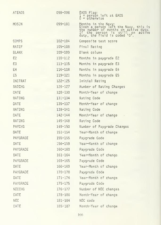
ATEAOS 098-098 EAOS Flag:1 = person left at EAOS

= otherwise

MOSIN 099-101 Months in the Navy:Given a person left the Navy, this isthe number of months on active duty.If the person is still on activeduty, the field is coded '0

.

COMPS 102-104 Composite test score

RATEF 105-108 Final Rating

BLANK 109-109 Blank column

E2 110-112 Months in paygrade E2




INITRAT 122-125 Initial Rating

RATCHG 126-127 Number of Rating Changes

DATE 128-130 Month-Year of change

RATING 131-134 Rating Code





PAYCHG 149-150 Number of Paygrade Changes

DATE 151-154 Year-Month of change

PAYGRADE 155-155 Paygrade Code









NECCHG 176-177 Number of NEC changes


NEC 181-184 NEC code


106

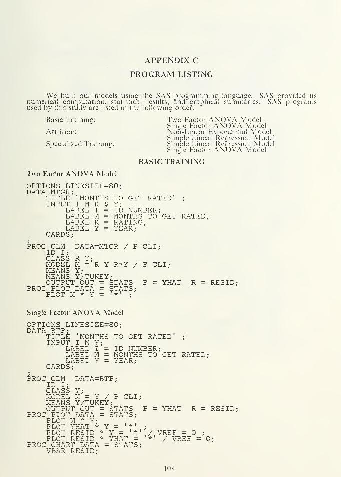
APPENDIX C

PROGRAM LISTING

We built our models using the SAS programming language. SAS r

numerical computation, statistical results, and graphical summaries. SA;used by this study are listed in the following order.

>rovided us! programs

Basic Training:

Attrition:

Specialized Training:

Two Factor ANOVA Model

Two Factor ANOVA ModelSingle Factor AXOVA ModelNon- Linear Exponential ModelSimple Linear Regression ModelSimple Linear Regression ModelSingle Factor ANOVA Model

BASIC TRAINING

OPTIONS LINESIZE=80;DATA MTGR;

TITLE 'MONTHS TO GET RATED'INPUT I M R $

LABEL I

LABEL MLABEL RLABEL Y

CARDS;

Y;ID NUMBER;MONTHS TO GET RATED;RATING;YEAR;

PROC GLM DATA=MTGR / P CLI;ID I;CLASS R Y*MODEL M ='R Y R*Y / P CLI;MEANS Y;MEANS Y/TUKEY;OUTPUT OUT = STATS P = YHAT R = RESID;

PROC PLOT DATA = STATS;PLOT M * Y = '

*' ;


OPTIONS LINESIZE=80;DATA BTP;

TITLE 'MONTHS TO GET RATED" ;

INPUT I M Y;LABEL I = ID NUMBER;LABEL M = MONTHS TO GET RATED;LABEL Y = YEAR;

CARDS;

PROC GLM DATA=BTP;ID I;CLASS Y;MODEL M = Y / P CLI;MEANS Y/TUKEY;OUTPUT OUT = STATS P = YHAT R = RESID;

PROC PLOT DATA = STATS;PLOT M * Y;PLOT YHAT * Y = ' *

' ;

PLOT RESID * Y = '*' / VREE = ;

PLOT RESID * YHAT = '*' / VREF = 0;PROC CHART DATA = STATS;

VBAR RESID;

108

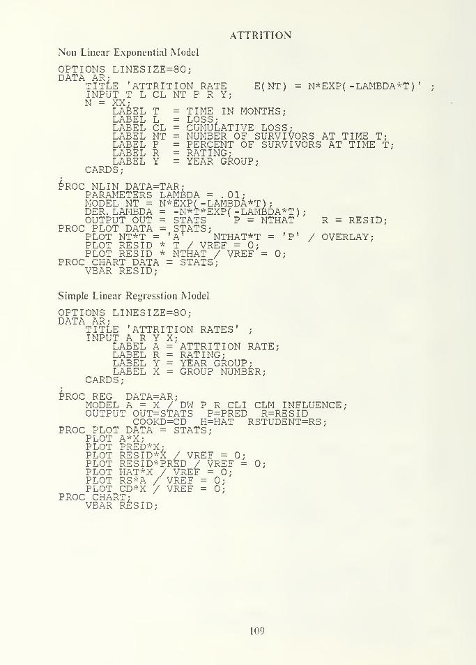
ATTRITION

Non Linear Exponential Model

OPTIONS LINESIZE=80;DATA AR

•

TITLE 'ATTRITION RATE E(NT) = N*EXP ( -LAMBDA* T)INPUT T L CL NT P R Y;N = XX;

LABEL T = TIME IN MONTHS;LABEL L = LOSS;LABEL CL = CUMULATIVE LOSS;LABEL NT = NUMBER OF SURVIVORS AT TIME T;LABEL P = PERCENT OF SURVIVORS AT TIME T;LABEL R = RATING;LABEL Y = YEAR GROUP;

CARDS;

PROC NLIN DATA=TAR;PARAMETERS LAMBDA = .01;MODEL NT = N*EXP( -LAMBDA*T)

;

DER. LAMBDA = -N*T*EXP( -LAMBDA*T )

;

OUTPUT OUT = STATS P = NTHAT R = RES ID;PROC PLOT DATA = STATS;

PLOT NT*T = 'A' NTHAT*T = 'P' / OVERLAY;PLOT RES ID * T / VREF = 0;PLOT RES ID * NTHAT / VREF = 0;

PROC CHART DATA = STATS;VBAR RES ID;

Simple Linear Regression Model

OPTIONS LINESIZE=80;DATA AR

•

TITLE 'ATTRITION RATES' ;

INPUT A R Y X;LABEL A = ATTRITION RATE;LABEL R = RATING;LABEL Y = YEAR GROUP;LABEL X = GROUP NUMBER;

CARDS;

PROC REG DATA=AR;MODEL A=X/DWPRCLI CLM INFLUENCE;OUTPUT OUT=STATS P=PRED R=RESID

COOKD=CD H=HAT RSTUDENT=RS;PROC PLOT DATA = STATS;

PLOT A*X;PLOT PRED*X;PLOT RESID*X / VREF = 0;PLOT RESID*PRED / VREF = 0;PLOT HAT*X / VREF = 0;PLOT RS*A / VREF = 0;PLOT CD*X / VREF = ;

PROC CHART;VBAR RES ID;

109

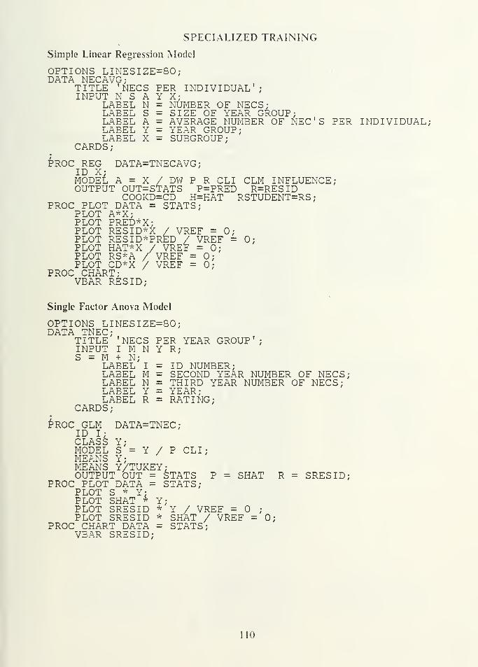
SPECIALIZED TRAINING

Simple Linear Regression Model

OPTIONS LINESIZE=80;DATA NECAVG;

TITLE 'NECS PER INDIVIDUAL';INPUT N S A Y X;

LABEL N = NUMBER OF NECS;LABEL S = SIZE OF YEAR GROUP;LABEL A = AVERAGE NUMBER OF NEC'S PER INDIVIDUAL;LABEL Y = YEAR GROUP;LABEL X = SUBGROUP;

CARDS;

PROC REG DATA=TNECAVG;ID X;MODEL A = X / DW P R CLI CLM INFLUENCE;OUTPUT OUT=STATS P=PRED R=RESID

COOKD=CD H=HAT RSTUDENT=RS;PROC PLOT DATA = STATS;

PLOT A*X;PLOT PRED*X;PLOT RESID*X / VREF = 0;PLOT RESID*PRED / VREF = 0;PLOT HAT*X / VREF = 0;PLOT RS*A / VREF = 0;PLOT CD*X / VREF = 0;

PROC CHART;VBAR RES ID;

Single Factor Anova Model

OPTIONS LINESIZE=80;DATA TNEC;

TITLE 'NECS PER YEAR GROUP';INPUT I M N Y R;S = M + N;

LABEL I = ID NUMBER;LABEL M = SECOND YEAR NUMBER OF NECS;LABEL N = THIRD YEAR NUMBER OF NECS;LABEL Y = YEAR;LABEL R = RATING;

CARDS;

PROC GLM DATA=TNEC;ID I;CLASS Y;MODEL S = Y / P CLI;MEANS Y;MEANS Y/TUKEY;OUTPUT OUT = STATS P = SHAT R = SRESID;

PROC PLOT DATA = STATS;PLOT S * Y;PLOT SHAT * Y;PLOT SRESID * Y / VREF = ;

PLOT SRESID * SHAT / VREF = 0;PROC CHART DATA = STATS;

VBAR SRESID;

110

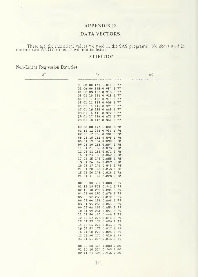
APPENDIX D

DATA VECTORS

These are the numerical values we used in the SAS programs. Numbers used inthe first two ANOVA models will not be listed.

ATTRITION

Non-Linear Regression Data Set

AT AW AX

00 00 00 131 1 .000 2 7701 06 06 125 ,954 2 7702 02 08 123 0.,938 2 7703 02 10 121 ,923 2 7704 01 11 120 ,916 Z 7705 01 12 119 ,908 2 7706 02 14 117 .893 2 7707 01 15 116 ,835 2 7708 01 16 115 ,877 2 7719 01 17 114 0.870 2 7720 01 18 113 0.862 2 77

00 00 00 173 1 ,000 2 7801 12 12 161 .930 2 7802 05 17 156 .901 2 7805 01 18 155 .895 2 7806 01 19 154 .890 2 7809 01 20 153 ,884 2 7811 01 21 152 .878 2 7812 01 22 151 .872 2 7816 01 23 150 .867 2 7817 02 25 148 .855 2 7818 01 26 147 .849 2 7820 01 27 146 .843 Z 7821 01 28 145 .838 2 7823 02 30 143 .826 z 7824 01 31 142 .820 2 78

00 00 00 330 1 .000 2 7901 19 19 311 .942 2 7902 19 38 292 .834 2 7904 02 40 290 .878 2 7905 02 42 288 .872 2 7906 02 44 286 .866 2 7903 01 45 285 .863 2 7909 03 48 282 .854 2 7910 01 49 281 .851 2 7911 01 50 280 .848 2 7912 02 52 278 .842 2 7913 01 53 277 .83 9 2 7914 02 55 275 .833 2 7915 02 57 273 .827 2 7916 01 58 272 .824 2 7922 02 60 270 .818 2 7923 01 61 269 .315 Z 79

00 00 00 324 1.000 2 8001 10 10 314 0.969 2 8002 11 21 303 0.935 2 80

111

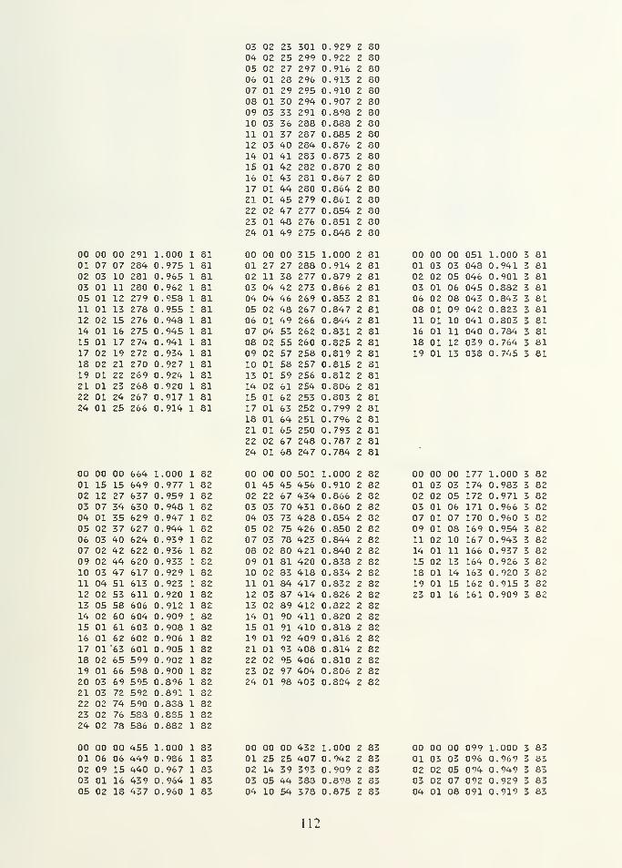
03 02 23 301 0.929 Z 8004 02 25 299 0.922 z 8005 02 27 297 0.916 2 8006 01 28 296 0.913 2 8007 01 29 295 0.910 2 8003 01 30 294 0.907 2 8009 03 33 291 0.898 2 8010 03 36 288 0.888 2 8011 01 37 287 0.885 2 8012 03 40 284 0.876 2 8014 01 41 283 0.873 2 8015 01 42 282 0.870 2 8016 01 43 231 0.867 2 8017 01 44 280 0.864 2 8021 01 45 279 0.861 2 8022 02 47 277 0.854 2 8023 01 48 276 0.851 2 8024 01 49 275 0.848 2 80

00 00 00 291 1..000 1 81 00 00 00 315 1.000 2 81 00 00 00 051 1 ,000 3 8101 07 07 284 0,.975 1 81 01 27 27 288 0.914 2 81 01 03 03 048 ,941 3 8102 03 10 281 0,.965 1 81 02 11 38 277 0.879 2 81 02 02 05 046 ,901 3 8103 01 11 280 ,962 1 81 03 04 42 273 0.866 2 81 03 01 06 045 ,882 3 8105 01 12 279 .953 1 81 04 04 46 269 0.853 2 81 06 02 08 043 ,843 3 8111 01 13 278 .955 1 81 05 02 48 267 0.847 2 81 08 01 09 042 ,823 3 8112 02 15 276 0.,943 1 81 06 01 49 266 0.844 2 81 11 01 10 041 ,803 3 8114 01 16 275 0.,945 1 81 07 04 53 262 0.831 2 81 16 01 11 040 ,784 Z 8115 01 17 274 ,941 1 81 08 02 55 260 0.825 2 81 18 01 12 039 0, , 7o4 Z 8117 02 19 272 0.,934 1 81 09 02 57 258 0.819 2 81 19 01 13 038 ,745 Z 8118 02 21 270 .927 1 81 10 01 58 257 0.815 2 8119 01 22 269 0,,924 1 81 13 01 59 256 0.812 2 8121 01 23 268 ,920 1 81 14 02 61 254 0.806 2 8122 01 24 267 0,,917 1 81 15 01 62 253 0.803 2 8124 01 25 266 0.,914 1 81 17

18212224

0101010201

6364656768

252251250248247

0.7990.7960.7930.7870.784

2

2

2

2

2

8181818181

00 00 00 664 1.,000 1 82 00 00 00 501 1.000 2 82 00 00 00 177 1 ,000 Z 8201 15 15 649 ,977 1 82 01 45 45 456 0.910 2 82 01 03 03 174 .983 z 8202 12 27 637 0.,959 1 82 02 22 67 434 0.866 2 82 02 02 05 172 ,971 3 8203 07 34 630 ,948 1 82 03 03 70 431 0.860 2 82 03 01 06 171 ,966 3 3204 01 35 629 ,947 1 82 04 03 73 428 0.854 2 82 07 01 07 170 ,960 Z 8205 02 37 627 ,944 1 82 05 02 75 426 0.850 2 82 09 01 08 169 ,954 Z 8206 03 40 624 ,939 1 82 07 03 78 423 0.844 2 82 11 02 10 167 ,943 Z 8207 02 42 622 ,936 1 82 08 02 80 421 0.840 2 82 14 01 11 166 .937 Z 8209 02 44 620 ,933 1 82 09 01 81 420 0.838 2 82 15 02 13 164 ,926 3 8210 03 47 617 ,929 1 82 10 02 33 418 0.834 2 82 18 01 14 163 .920 3 8211 04 51 613 ,923 1 82 11 01 84 417 0.832 2 82 19 01 15 162 .915 3 8212 02 53 611 ,920 1 82 12 03 87 414 0.826 2 82 23 01 16 161 ,909 3 8213 05 58 606 ,912 1 82 13 02 89 412 0.322 2 8214 02 60 604 ,909 1 82 14 01 90 411 0.820 2 8215 01 61 603 ,903 1 82 15 01 91 410 0.818 2 8216 01 62 602 ,906 1 82 19 01 92 409 0.816 2 8217 01 '63 601 ,905 1 82 21 01 93 408 0.814 2 8218 02 65 599 .902 1 82 22 02 95 406 0.810 2 8219 01 66 598 .900 1 82 23 02 97 404 0.806 2 8220 03 69 595 0..896 1 82 24 01 98 403 0.804 2 8221 03 72 592 .891 1 8222 02 74 590 ,838 1 8223 02 76 583 .885 1 8224 02 78 586 .882 1 82

00 00 00 455 1.000 1 8301 06 06 449 0.986 1 8302 09 15 440 0.967 1 8303 01 16 439 0.964 1 8305 02 18 437 0.960 1 83

00 00 00 432 1.000 2 8301 25 25 407 0.942 2 8302 14 39 393 0.909 2 8303 05 44 388 0.898 2 8304 10 54 378 0.875 2 83

00 00 00 099 1,

01 03 03 096 0,

02 02 05 09403 02 07 09204 01 08 091

000 3 83969 3 83949 3 83929 3 83919 3 83

112

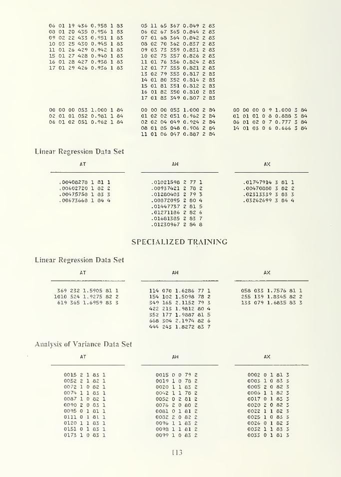
06 01 19 436 0,.958 1 83 05 11 65 367 ,849 2 8308 01 20 435 0.,956 1 83 06 02 67 365 ,844 2 8309 02 22 433 0. 951 1 83 07 01 68 364 ,842 2 8310 03 25 430 0.,945 1 83 08 02 70 362 ,837 2 8311 01 26 429 0.,942 1 83 09 03 73 359 ,831 2 8315 01 27 428 0.,940 1 83 10 02 75 357 ,826 2 8316 01 28 427 0.,938 1 83 11 01 76 356 .824 2 8317 01 29 426 0.,936 1 83 12

13141516

17

010201010101

777980818283

355353352351350349

.821

.817

.814

.812

.810

.807

2 832 832 832 832 832 83

00 00 00 053 1.000 1 8402 01 01 052 0.981 1 8406 01 02 051 0.962 1 84

00 00 00 053 1.000 2 8401 02 02 051 0.962 2 8402 02 04 049 0.924 2 8408 01 05 048 0.906 2 8411 01 06 047 0.887 2 84

00 00 00 9 1.000 3 8401 01 01 8 0.888 3 8406 01 02 7 0.777 3 8414 01 03 6 0.666 3 84

Linear Regression Data Set

AT AW

.00408278 1 81 1 .01021598 2 77 1

.00602720 1 82 2 .00937421 2 78 2

.00475758 1 83 3 .01280403 2 79 3

.00673668 1 84 4 .00872095 2 80 4.01447737 2 81 5.01271186 2 82 6

.01681385 2 83 7

.01230967 2 84 8

AX

.01747914 3 81 1

.00470880 3 82 2

.02313339 3 83 3

.03262699 3 84 4

SPECIALIZED TRAINING

Linear Regression Data Set

AT

369 232 1.5905 81 1

1010 524 1.9275 82 2

619 365 1.6959 83 3

AW

114 070 1 ,6286 77 1

154 102 1 ,5098 78 2

349 165 2 ,1152 79 3

422 213 1.,9812 80 4352 177 1,,9887 81 5668 304 2 ,1974 82 6

444 243 1 ,8272 83 7

AX

058 033 1.7576 81 1

255 139 1.8345 82 2

133 079 1.6835 83 3

Analysis of Variance Data Set

AT AW AX

0015 2 1 83 1 0015 79 2 0002 1 81 3

0052 2 1 82 1 0019 1 78 2 0003 1 83 3

0072 1 82 1 0020 1 1 83 2 0005 2 82 3

0074 1 1 83 1 0042 1 1 78 2 0006 1 l 82 3

0087 1 82 1 0052 2 81 2 0017 l 83 3

0090 2 83 1 0076 2 80 2 0020 2 82 3

0095 1 81 1 0081 1 81 2 0022 1 1 82 3

0111 1 81 1 0032 2 82 2 0025 1 83 3

0120 1 1 83 1 0096 1 1 83 2 0026 1 82 3

0151 1 83 1 0098 1 1 81 2 0032 1 1 83 3

0173 1 83 1 0099 1 83 2 0033 1 81 3

113

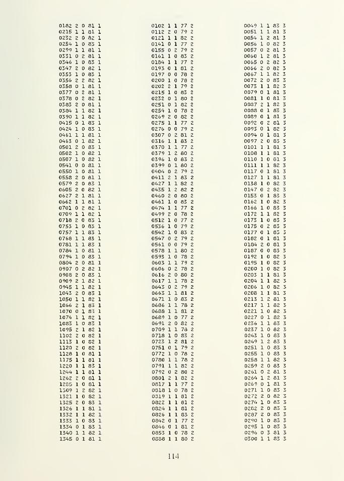
0182 2 81 1

0215 1 1 81 1

0232 2 82 1

0254 1 83 1

0299 1 1 81 1

0331 2 81 1

0346 1 83 1

0347 2 82 1

0353 1 83 1

0356 2 2 82 1

0358 1 81 1

0377 2 81 1

0378 2 82 1

0383 2 81 1

0384 1 1 82 1

0390 1 1 82 1

0415 1 83 1

0424 1 83 1

0461 1 1 81 1

0463 1 82 1

0501 2 83 1

0502 1 32 1

0507 1 82 1

0541 81 1

0550 1 81 1

0558 2 81 1

0579 2 83 1

0605 2 82 1

0627 2 1 81 1

0662 1 1 81 1

0701 2 82 1

0709 1 1 82 1

0718 2 83 1

0753 1 83 1

0757 1 1 83 1

0768 1 1 83 1

0781 1 1 83 1

0784 1 81 1

0794 1 83 1

0804 2 81 1

0907 2 82 1

0903 2 83 1

0909 2 1 82 1

0945 1 1 82 1

1043 2 83 1

1050 1 1 82 1

1066 2 1 83 1

1070 1 83 1

1074 1 1 82 1

1083 1 83 1

1095 2 1 82 1

1102 2 82 1

1113 1 82 1

1120 2 82 1

1128 1 81 1

1175 1 1 81 1

1220 1 1 83 1

1244 1 1 81 1

1262 2 81 1

1285 1 81 1

1309 1 2 82 1

1321 1 82 1

1325 2 83 1

1326 1 1 81 1

1332 1 1 82 1

1333 1 83 1

1334 1 83 1

1340 1 1 82 1

1345 1 81 1

0102 1 1 77 2

0112 2 79 2

0121 1 1 82 2

0141 1 77 2

0155 2 79 2

0161 1 83 2

0184 1 1 77 2

0193 1 81 2

0197 78 2

0200 1 78 2

0202 2 1 79 2

0215 1 83 2

0232 1 80 2

0251 1 82 2

0254 1 78 2

0269 2 82 2

0275 1 1 77 2

0276 79 2

0307 2 81 2

0316 1 1 83 2

0370 1 1 77 2

0379 1 2 80 2

0396 1 83 2

0399 1 80 2

0404 2 79 2

0411 2 1 83 2

0427 1 1 82 2

0435 1 2 82 2

0460 2 80 2

0461 1 83 2

0474 1 1 77 2

0499 2 78 2

0512 1 77 2

0536 1 79 2

0542 1 83 2

0547 2 79 2

0561 79 2

0578 1 1 80 2

0593 1 78 2

0603 1 1 79 2

0606 2 78 2

0616 2 80 2

0617 1 1 78 2

0643 2 79 2

0663 1 1 81 2

0671 1 83 2

0686 1 1 78 2

0688 1 1 81 2

0689 1 77 2

0691 2 82 2

0709 1 1 78 2

0718 1 83 2

0723 1 2 81 2

0751 1 79 2

0772 1 78 2

0780 1 1 78 2

0791 1 1 82 2

0792 2 80 2

0801 2 1 82 2

0817 1 1 77 2

0818 1 78 2

0319 1 1 81 2

0822 1 1 81 2

0824 1 1 81 2

0826 1 1 83 2

0842 1 77 2

0846 1 81 2

0853 1 78 2

0888 1 1 80 2

004900510054005600570060006500660067007200730079008100370083008900920093009400970101010801100111011701270138014701530162016601720173017501770182018401870192019502000203020402060208021302170221022702360237024302490251025502580259026102640269027102720274028202870290029502960300

114

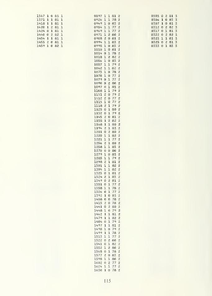
1367 1 83 1

1371 1 1 81 1

1418 1 1 81 1

1420 1 z 81 1

1424 1 81 1

1440 z 82 1

1454 1 1 81 1

1455 2 81 1

1459 1 82 1

0897 1 1 81 2

0926 1 1 78 2

0949 1 83 2

0954 1 1 77 2

0969 1 1 77 2

0971 1 2 80 2

0988 2 81 2

0994 1 1 83 2

0993 1 83 2

1010 1 81 2

1014 1 78 2

1018 1 2 82 2

1056 1 83 2

1057 1 1 79 2

1062 1 1 82 2

1073 1 78 2

1078 1 77 2

1079 1 77 2

1090 2 80 2

1097 1 83 2

1108 1 1 79 2

1111 2 79 2

1112 2 77 2

1113 1 77 2

1118 2 1 79 2

1125 1 80 2

1132 1 79 2

1145 2 81 2

1155 1 2 82 2

1168 1 1 80 2

1194 2 1 83 2

1201 2 80 2

1220 1 1 82 2

1221 1 1 77 2

1256 2 1 80 2

1258 1 1 83 2

1270 80 2

1279 1 83 2

1285 1 1 79 2

1298 2 1 81 2

1301 1 1 82 2

1304 1 1 82 2

1323 1 81 2

1324 2 1 83 2

1349 2 81 2

1351 1 77 2

1358 1 1 78 2

1386 1 77 2

1392 1 83 2

1408 78 2

1415 2 78 2

1441 2 80 2

1448 1 79 2

1462 1 1 81 2

1479 1 1 82 2

1484 1 79 2

1497 1 1 81 2

1498 1 79 2

1499 1 1 78 2

1513 1 1 77 Z

1522 2 80 2

1541 1 82 2

1552 1 2 80 2

1568 1 78 2

1577 2 83 2

1598 1 1 80 2

1602 2 77 2

1624 1 1 77 2

1630 1 78 2

0303 2 81 3

0306 1 83 3

0307 1 81 3

0312 2 82 3

0317 1 81 3

0322 2 82 3

0323 1 1 81 3

0325 2 81 3

0333 1 83 3

115

1641 1 80 2

1642 1 1 79 2

1652 2 80 2

1666 1 77 2

1673 1 1 82 2

1693 1 83 2

1711 1 2 80 2

1721 1 81 2

1729 1 80 2

1730 1 81 2

1736 1 1 81 2

1749 1 80 2

1757 1 1 82 2

1761 1 1 77 2

1763 1 81 2

1766 1 78 2

1777 1 2 79 2

1782 1 2 82 2

1786 2 77 2

1783 2 83 2

1804 2 82 2

1821 1 1 83 2

1827 1 1 77 2

1831 1 1 82 2

1860 1 2 81 2

1874 2 81 2

1879 1 78 2

1884 2 82 2

1895 1 2 81 2

1908 1 1 77 2

1928 1 78 2

1945 2 1 79 2

1970 1 2 79 2

1974 2 80 2

1975 1 77 2

1978 2 82 2

1986 1 77 2

1989 1 79 2

1992 1 77 2

2008 1 2 82 2

2018 1 2 82 2

2047 1 80 2

2053 1 1 79 2

2125 2 82 2

2163 1 82 2

2164 1 2 81 2

2179 2 83 2

2181 1 78 2

2184 80 2

2188 1 2 83 2

220001 79 2

2204 78 2

2206 3 80 2

2209 2 83 2

2215 1 81 2

2217 1 82 2

2231 1 1 82 2

2241 2 73 2

2255 2 1 80 2

2260 2 1 79 2

116

LIST OF REFERENCES

1. Corliss, George R., CNA Research Memorandum 86-3 "Non Prior ServiceAccession Daia Set," Alexandria, Virginia, Center for Xaval Analyses, 19S6.

2. Neter, John, Wasserman, William, and Kutner, Michael H., Applied LinearStatistical Models, Richard D. Irwin, Inc., 19S5.

3. Conover, W.J., Practical Nonparametric Statistics, John Wiley and Sons, Inc.,1980.

4. Draper, N.R. and Smith, H., Applied Regression Analysis, John Wiley andSons, Inc., 19S1.

5. Judge, Georse G., Hill, R. Carter, Griffiths, William E., Liitkepohl, Helmut,,and Lee, Tsoung-Chao, Introduction to the Theory and Practice ofEconometrics, JohifWilev and Sons, Inc., 1982

117

BIBLIOGRAPHY

Barr, Donald R. and Zehna, Peter W., Probability. Modeling Uncertainty,Addison-Wesley Publishing Company, 1983.

Box, George E.P.. Hunter, William G., and Hunter, J. Stuart, Statistics forExperimenters, John Wiley and Sons, Inc., 1978.

Chambers, John M.. Cleveland, William S., Kleiner, Beat, and Tukey, Paul A.,Graphical Methods for Data Analysis, Wadsworth International Group, Belmont,California, 1983

Gilman, Leonard and Rose. Allen J., APL An Interactive Approach, Third Edition,John Wiley and Sons, Inc., 1984.

Kreitzbers. Charles B. and Shneiderman, Ben, Fortran Programming, Second Edition,Harcourt "Brace Jovanovich, Inc., 1982.

Mosteller. Frederick and Tukey, John W., Data Analysis and Regression,Addison-Wesley Publishing Company, 1977.

Questor, Aline O. and Corliss. Georee R., CNA Research Memorandum S6-84 "Thehaw Enlisted Classification (NEC's): A History"', Alexandria, Virginia, Center for NavalAnalyses, 1986.

Questor, Aline O., Byrnes, Patricia E., Corliss, Georce R., Dorsey, Cheryl A., Hill,

John L., and Schoeck, Susan \1. CNA Research Memorandum' 86-90 /SpecializedTraining for Enlisted Navy Personnel: A Historical Account", Alexandria, Virginia,Center Tor Naval Analyses, 1986.

Ramsey % James B. and Musgrave, Gerald L., APL STAT, Lifetime LearningPublications, 1981.

SAS Institute Inc., SAS User's Guide Basics, Version 5 Edition, Cary, North Carolina,1985.

SAS Institute Inc., SAS User's Guide Statistics, Version 5 Edition, Cary, NorthCarolina, 1985.

118

INITIAL DISTRIBUTION LIST

No. Copies

1. Defense Technical Information Center 2Cameron StationAlexandria, Virginina 22304-6145

2. Librarv. Code 0142 2Naval "Postgraduate SchoolMonterey, California 93943-5000

3. Professor Dan C. Boger, Code 55Bo 1

Naval Postgraduate SchoolMonterey, California 93943-5000

4. Professor Robert R. Read, Code 55Re 1

Naval Postgraduate SchoolMonterey, California 93943-5000

5. Center for Naval Analyses 24401 Ford AvenuePost Office Box 16268Alexandria, Virginia 22302-0268

6. Lieutenant Kappv Aiu 24855-C Nonou RoadKapaa, Kauai, Hawaii 96746

119

«TITLE NUMBER .CUSTOMER NUMBER

Library, Naval Postgraduate SchLIBRARY _.

Binding in

Everything

:CONTENTS

! INDEX

' Bind without Index

;ISSUE CONTENTS

jDiscard

jBind in Place

1 Gather at Front

Advertisements

Front Covers

iBack Covers

1

1st only

Accents

Imprints

F B NP

IN OUT

EUGENE KAPUA AIU

Thesis A3306

Special Instructions

RosweLLbOOl<blNt)lNQLIBRARY DIVISION

Buck Color 2614 NORTH 29th AVENUEPHOENIX. ARIZONA 85009PHONE (602) 272-9338Print Color

Trim Height

Ht Inches

Over Thick

For Title

Extra Lines'-

Extra Coll

Hand Sew

Slit ACTUAL TRIM DATE

Rules

1st Slot No

Vol Slot No SPINE JOB

Year Slot No

Call # Slot

Imp Slot No BOARD DIM LOT

Type Face

Price

Mending CLOTH DIM ROUTE

Map Pockets

2 Vols in 1

CLOTH BIN SEQ NO

DUDLEY K

NAVA.I: :F00L nM

MO5°°

AiuA search for factors

causing training costs

to rise by examining the

U.S. Navy's AT, AW, and

AX ratings during their

first enlistment period.

Thesis

A3 30 6

c.l

21950C

AiuA search for factors

causing training costs

to rise by examining the

U.S. Navy's AT, AW, and

AX ratings during their

first enlistment period.

Documents

A search for factors causing training costs to rise by