A Sectoral Analysis of the 1929 Stock Market Crash

Claremont CollegesScholarship @ Claremont

CMC Senior Theses CMC Student Scholarship

2017

A Sectoral Analysis of the 1929 Stock Market CrashPaul Edward Reynolds IIIClaremont McKenna College

This Open Access Senior Thesis is brought to you by Scholarship@Claremont. It has been accepted for inclusion in this collection by an authorizedadministrator. For more information, please contact [email protected].

Recommended CitationReynolds, Paul Edward III, "A Sectoral Analysis of the 1929 Stock Market Crash" (2017). CMC Senior Theses. 1487.http://scholarship.claremont.edu/cmc_theses/1487

http://scholarship.claremont.edu

http://scholarship.claremont.edu/cmc_theses

http://scholarship.claremont.edu/cmc_student

mailto:[email protected]

Claremont McKenna College

A Sectoral Analysis of the 1929 Stock Market Crash

SUBMITTED TO

MARC WEIDENMIER

BY

PAUL EDWARD REYNOLDS III

FOR

SENIOR THESIS

FALL 2016

DECEMBER 5, 2016

Table of Contents

Introduction……………………………………………………………………………………………1

Literature Review…………………………………………………………………………………...3

Data…………………………………………………………………………………………………….….8

Empirical Strategy……….............................................................................10

Result……………………………………………………………………………………………………11

Conclusion…………………………………………………………………………………………….29

Works Cited…………………………………………………………………………………………..31

Abstract

The stock market crash of 1929 stands today as the largest decline in market

value in the history of the United States. Consequently, the event destroyed the

wealth of thousands of American families and institutions. On October 28th and

29th, the United States stock market fell 11.3 percent and 12.4 percent

respectively, marking the beginning of a down market that lasted over three years,

the time period known today as the Great Depression. This paper empirically

analyzes the effects felt by each individual industry sector in the crash of 1929,

identifying gross and abnormal returns over three major days in the crash. I then

compare my findings to previous literature and economic theories, analyzing

which sector returns were expected and which were abnormal.

1

1.) Introduction

The stock market crash of 1929 stands alone as the largest fall of market

value in United States history. Marking the beginning of the Great Depression, the

U.S. plunged into a state of panic from its previous period of rapid growth and

positivity during the “Roaring Twenties” (Pettinger, 2007). Known as “Black

Monday” and “Black Tuesday”, the market fell 11.2 percent and 11.9 percent

respectively. From its peak in mid-September of 1929 to halfway through 1932,

the market lost over 85 percent of its value.

While there have been studies that have explored the reasons for the 1929

stock market crash (see for example, Galbraith 1954 and Bierman 1998), to the

best of my knowledge, no empirical research on sector performance during the

1929 crash has been conducted. This is probably due to the lack of daily stock

data for 1929. With daily data now available on 17 sectors daily dating back to

1926 (French, 2016), I can analyze the effects of the Great Crash of 1929 on

different sectors of the stock market.

I use data on the daily stock returns for each sector leading up to and

following the crash in October of 1929. I focus on three specific days, October

28th, 29th, and 30th of 1929, because each of these days had a market swing of over

10 percent. Unlike earlier literature that provides a general summary of the effects

felt by various industrial sectors, I employ standard event study techniques in

finance to measure gross and abnormal returns for all 17 sectors.

My study yields the gross and abnormal returns for each separate industry

sector. For the 3-day cumulative gross returns from October 28th to October 30th,

1929, the sectors least affected were Construction (negative 7.99 percent),

2

Transportation (negative 8.06 percent), and Consumer Goods (negative 8.09

percent). Sectors impacted the most were Chemicals (negative 20.30 percent),

Finance (negative 18.94 percent), and Machines (negative 16.69 percent). These

returns are compared to the overall market which fell 12.45 percent. For the 3-day

cumulative abnormal returns, the top performers were Cars (positive 5.03

percent), Construction (positive 4.88 percent), and Consumer Goods (positive

2.69 percent). The worst performers were Chemicals (negative 5.85 percent),

Retail (negative 5.43 percent), and Mines (negative 5.22 percent). My findings

allow me to use empirical analysis to compare individual industry sector

performance across 17 sectors, using the results to explain variations in

performance versus previous economic literature and arguments.

3

2. Literature Review

There are many theories surrounding the causes for the Stock Market

Crash of 1929. Galbraith (1954) argues that one major reason for the

occurrence of the crash was the incredible speculation on the New York Stock

Exchange. He states that as the boom began in the early years of the 1920’s,

individuals as well as institutional investors began to greatly increase their

trading activity. This increase in activity caused a rise in stock values across

the board, building up to a culture of Americans buying large volumes of

stocks not for their returns, but rather for quick resale at inflated prices

(Galbriath, 1954). To make the situation worse, the speculative trading was

largely done on credit, creating a massive underlying bubble that was waiting

to pop. Thus, when the stock market began to turn grim in the fall of 1929,

stockbrokers were required to issue margin calls, which caused panic selling

that resulted in the tumbling of the stock market. While Galbraith (1954) does

no empirical analysis on different sectors of the market during 1929, he does

speak to the effect it had on the purchasing power of individuals of the time.

He states that the crash resulted in consumers cutting purchases, manufacturers

cutting back production, and employers choosing to lay-off workers. The

financial sector was brought down with their issues of credit, and that resulted

in the bankruptcy of many banks. The economy was left in a state where

money was tight and purchasing power was low.

White (1989) revisits the United States stock market crash of 1929 by

compiling numerous sources focused on the catalysts of the crash. He suggests

that speculation was indeed a factor because of America’s use of credit and

investment trusts, contributing to higher trading activity and high valuations of

4

stocks. He attributes market fundamentals as the initial cause of the bubble, but

goes on to argue that they were never strong enough to sustain the rapid growth

in valuations of stocks. He cites the work of Sirkin (1975), that stated that high

stock prices and high price-to-earnings ratios were a consequence of expected

rapid growth of earnings. In particular, White (1989) shows this by creating a

graph of stock prices vs. dividends for all the major companies in the Dow-

Jones Index from 1926 – 1929. Leading up to 1928, there was a minimal gap

between the two, but from 1928 – 1929, the gap increased massively. The start

of this increase was attributed by White (1989) to when the market was

becoming over-valued. He explains how the increase in stock prices vs. the

hesitancy of managers to increase dividends meant that the managers knew that

their revenue growth was not sustainable, showing that they did not share the

same enthusiasm as the general public. He also shares that previous economists

have argued that the crash began in the public utilities sector, which was

extremely popular at the time and had experienced massive growth leading up

to October, but he says that there is not enough evidence for proof of this

theory.

Bierman (1998) explores the reasons for the “Great Crash” in an attempt

to give the reader a better understanding of the events that unfolded during the

last days of October, 1929. He highlights that speculation was the common

belief for the explanation of the crash during that time period, (see for example,

Keynes 1930 and Hoover 1950), but he did not agree with this explanation. He

states that one major reason to reject the belief of speculation is to study the

reactions of leading economists of the time. Specifically, he shows that both

Irving Fisher and John Maynard Keynes, considered leading economists of the

1920’s, were bullish before and after the crash in October, 1929. Neither

profited from their views, and lost heavily over the crashing market. Therefore,

5

the belief is that it was not just “fools” and speculators that drove stock prices

up, but rather economic indicators that supported their growth.

Bierman (1998) also touches on the growth and expansion of investment

trusts as a reason for the crash. He takes an article from The Economist in 1929

that reported that $1 billion of investment trusts were sold in the first 8 months

of 1929, compared to the entire year of 1928’s total of $400 million,

illustrating their increasing popularity. These trusts acted similar to the mutual

funds of today, where small investors were able to pool their money in order to

achieve greater diversification. The problem with these trusts was that they

were highly levered, and were particularly vulnerable to stock price declines.

At the time, these trusts were considered reliable because of their experienced

management and ability to diversify portfolios, but a diversification of stocks

during that time period could not stand the burden of large universal price

declines. Bierman (1998) goes on to explain how certain information would be

extremely helpful in order to better explain the effects caused by investment

trusts. He states that information such as the percentage of the portfolio that

were public utilities, the extent of their diversification, the percentage of

portfolios that were NYSE firms, and the amount of debt and preferred stock

leverage used would be extremely insightful.

To the best of my knowledge, however, there are no papers specifically

examining the sectoral effects in 1929. Despite this, one can gain some insight

on the sectoral effects from the aforementioned discussed thus far. Bierman

(1998) states that during the time leading up to October, 1929, stock prices did

not rise across all industries. He explains that stock prices rose most in

industries where economic fundamentals illustrated a reason for public

optimism. These sectors included airplanes, agriculture, chemicals, department

stores, steel, utilities, telephones/telegraph, electrical equipment, oil, paper, and

6

radio. Richardson (2013) also concluded that automobiles, telephones, and

other new technologies were experiencing rapid growth leading up to the crash.

Due to their success and expansion during the 1920’s, Bierman (1998) comes

to the conclusion that these were reasonable choices for further sectoral

growth. In his writing, he focuses specifically on public utilities, citing

Wigmore (1985) who concluded that at the time of the crash the sector was

trading at three times its book value, an indication he argued hinted at a bubble.

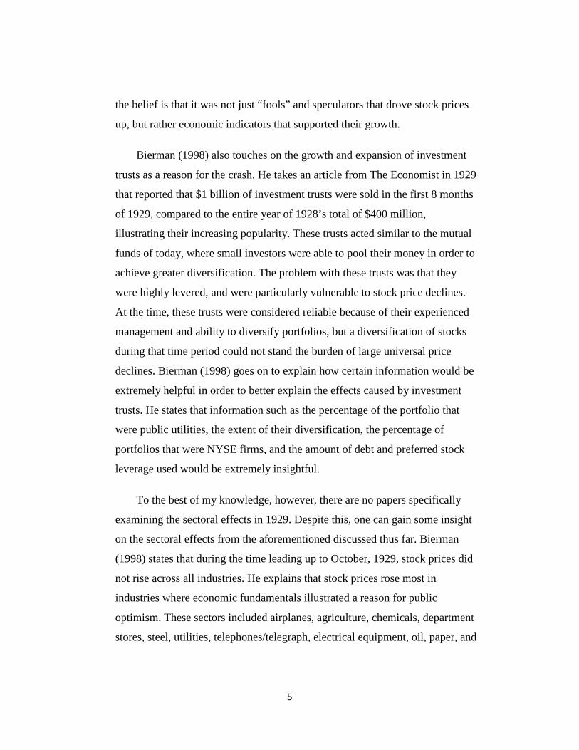
I attached below a graph of individual sector value in the nine months

leading up to the crash. I created this graph using the daily returns given by

Kenneth French’s 17 Industry Portfolio sample for each industry sector starting

in January of 1929. The purpose of this graph is to illustrate the sectors that

were experiencing high growth leading up to the crash. The graph illustrates

how sectors such as Utilities, Machines, and Chemicals were experiencing very

high growth in the months leading up to the crash, while industries such as

Cars and Cloths were experiencing significant losses.

7

Figure 1.

Data taken from Kenneth French’s 17 Industry Portfolio’s (French, 2016)

The goal of this paper is to research the returns of each sector during this stock

market crash, and provide an explanation for abnormal returns across the market.

While economists focused mainly on the Public Utility and Financial sectors

during the crash, this paper will expand the research to 17 sectors during the 1929

stock crash, explicitly examining the returns of each individual one.

0

20

40

60

80

100

120

140

160

180

200

Jan Feb Mar April May Jun July Aug Sep

Sector ValueJanuary 1929 - September 1929

Food Mines Oil Cloths Durables ChemicalsConsumer Construction Steel Fabric Products Machines CarsTransportation Utilities Retail Finance Other Market

8

3.) Data

I use data from Kenneth French’s 17 Industry Portfolios sample (French,

2016). The data set is ideal for my purposes because it tracks the daily returns of

17 sectors from 1926 through 2015 in the United States. I argue that the 17

industry sectors accurately divide and capture the entire U.S. financial market

during this time period. The industry sectors variables include; Food, Mines

(Mining and Minerals), Oil (Oil and Petroleum products), Clothes (Textiles,

Apparel & Footwear), Durables (Consumer Durables), Chemicals (Chemicals),

Consumer (Drugs, Soap, Perfumes, Tobacco), Construction (Construction and

Construction Materials), Steel (Steel Works etc.), Fabricated Products, Machinery

(Machinery and Business Equipment), Cars (Automobiles), Transportation,

Utilities, Retail (Retail Stores), Finance (Banks, Insurance Companies, and Other

Financials), and Other. I created 3 dummy variables to account for the two days

where the market experiences extreme losses, October 28th and 29th, as well as the

following day of October 30th, where the market experienced a massive recovery

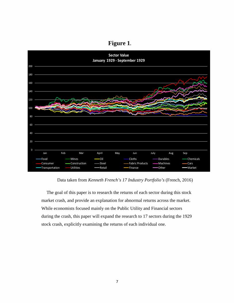
gain. Attached below are the summary statistics I gathered from French’s data set

of the three major days of extreme market returns versus the 17 industry sectors as

a whole. Table 1 illustrates how there was a wide range of returns posted across

all the industry sectors.

9

Table 1. Sample Statistics: Industry Sectors vs. Market Returns


Date28-Oct-29 29-Oct-29 30-Oct-29

Market Return (0.1127) (0.1199) 0.1218

Sector Return Mean (0.1112) (0.1162) 0.1113

Standard Error 0.0095 0.0108 0.0108

Median Return (0.1073) (0.1207) 0.1204

Standard Deviation 0.0392 0.0445 0.0445

Sample Variance 0.1533 0.1978 0.1983

Range 0.1491 0.1842 0.1796

Minimum (0.1729) (0.1917) 0.0272

Maximum (0.0238) (0.0075) 0.2068

10

4.) Empirical Strategy

To formally test the effects of the crash on each industry sector, I examine each

sector individually and compare it to the market in terms of its gross returns and

impact of the three major days of the market crash. Thus, the return for each

industry sector is estimated from a linear regression of the following form

(1) 𝑆𝑆𝑖𝑖 = α + β𝑚𝑚𝑚𝑚𝑚𝑚 + β𝑑𝑑1 + β𝑑𝑑2 + β𝑑𝑑3 + ℇ𝑖𝑖

where Si is the return for the specific industry sector, mkt is the market return, d1

is a dummy variable accounting for October 28th, 1929, d2 is a dummy variable

accounting for October 29th, 1929, and d3 is a dummy variable accounting for

October 30th, 1929.

11

5.) Results

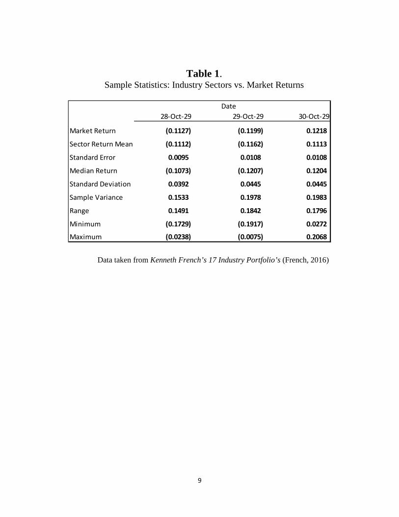
The following pages explore my results for each individual industry sector’s

performance versus the market. Table 2 below describes the results found through

each regression of the respective industry sector. This table also illustrates the

impact of each date I analyzed using dummy variables and the coefficients they

produced. The coefficients of the three specific days explains the abnormal

returns for that industry sector on that specific day. The table is sorted by the 3-

day abnormal return for each sector, starting from the worst overall abnormal

return. The 3-day abnormal return was calculated using the sum of the three

coefficients from the three days that I am studying. As the economists I

referenced suggested, the utilities industry sector had been experiencing extreme

growth leading up the crash, but what is interesting is that the abnormal returns

for that sector for each individual day were not too extreme. Utilities largest

abnormal return was just over 3 percent, on October 29th, suggesting that overall

the sector’s performance was mostly in-line with market expectations. The same

can be said for the Oil and Steel sectors, where their abnormal returns were

comparatively minimal. On the other hand, a few of the industries experienced

massive abnormal returns during these three days. Construction for example took

a huge hit on the first day, October 28th, posting an abnormal negative return of

over 6.3 percent. The next day, it posted an even bigger abnormal return of over

10 percent, except this time it was in the positive direction. On October 29th, the

Mining sector took the largest hit, posting a negative abnormal return of over 8

percent. For the last day, the two sectors that posted the biggest abnormal returns

were the Durables and Cars sectors. Durables posted a negative abnormal return

of over 7.3 percent on October 30th, which is not surprising given the nature of

durable goods in a tight market. What is surprising is the abnormal positive return

12

of the Cars sector of over 7 percent, since the automobile industry is composed of

high ticket items. The abnormal returns of each date and sector can be found

below.

Table 2. Linear Regression Output


Mkt Beta Standard Deviation Oct 28 (Coef.) Oct 29 (Coef.) Oct 30 (Coef.) 3-Day Ab Return α

Industry Sector

Chemicals 1.1449 0.0666 (0.0142) (0.0548) 0.0106 (0.0583) 0.0003

Retail 0.8830 0.0343 (0.0008) (0.0098) (0.0437) (0.0543) (0.0010)

Mines 0.3950 0.0822 0.0211 (0.0847) 0.0114 (0.0522) (0.0004)

Cloths 0.5384 0.0627 0.0058 (0.0057) (0.0368) (0.0367) (0.0015)

Machines 1.1123 0.0481 (0.0248) 0.0064 (0.0139) (0.0323) 0.0004

Fabrics 1.0844 0.0884 (0.0022) (0.0146) (0.0102) (0.0270) 0.0003

Finance 1.2574 0.0773 (0.0141) (0.0232) 0.0136 (0.0238) (0.0011)

Other 1.0031 0.0508 (0.0213) 0.0067 (0.0026) (0.0172) 0.0008

Durables 1.3244 0.1595 0.0420 0.0264 (0.0731) (0.0047) (0.0000)

Transportation 0.6798 0.0368 0.0051 0.0119 (0.0202) (0.0033) 0.0005

Steel 0.9805 0.0625 0.0113 0.0179 (0.0212) 0.0081 0.0002

Food 0.8969 0.05241 (0.0035) (0.0134) 0.0288 0.0119 0.0003

Oil 0.9576 0.0991 0.0218 0.0131 (0.0158) 0.0191 0.0008

Utilities 1.3258 0.0612 (0.0030) 0.0337 (0.0114) 0.0193 (0.0001)

Consumer 0.9206 0.2072 0.0129 0.0313 (0.0173) 0.0269 0.0009

Construction 0.9704 0.07978 (0.0634) 0.1090 0.0027 0.0483 (0.0001)

Cars 1.1418 0.103 0.0115 (0.0313) 0.0702 0.0503 (0.0024)

13

Table 3 focuses on the gross returns of each industry sector versus the market.

The first three columns are the returns for each individual day of the crash. The

fourth column describes the 3-day gross return of each industry sector for the

period of October 28th through the 30th. The table is sorted by sector performance

based on its 3-day gross return, starting with the worst individual industry

performance which was Chemicals.

The performance of the Chemicals sector is interesting because of the lack of

attention it was given by previous literature. Posting an overall 3-day negative

gross return of more than 20 percent, the sector took the largest dip out of all of

the 17, but the reaction of this sector is expected in a downturn of an economy.

The second worst performing industry sector was Finance. I expected this because

of previous literature and because a large negative reaction to the Finance sector

is common in financial crisis’s. Other sectors that fell in-line with my

expectations were the Consumer Goods and Oil sectors. Since these industries are

composed of goods that are necessities, their solid performance compared to the

market was not unexpected. Two industries predicted to feel large negative effects

were the Utilities and Durables sectors. Surprisingly, even though both sectors

lost roughly 15 percent of their value over the 3-day period, their returns were not

comparatively abnormal and very in-line with market expectations. The focus of

Bierman (1998) and White (1989) on the Utilities sector made me anticipate a

greater negative return by the industry. The most surprising performance was the

Construction sector. Construction performed the best compared to the other 16

sectors, posting a 3-day negative gross return of only 8 percent. Perhaps this can

be explained by the industry sector’s performance leading up to the crash. Shown

in Figure 1, Construction performed well below the market in the months leading

up to the crash. Therefore, there is a possibility that the market had already

adjusted for a decline in the Construction sector and as a result, the crash’s impact

was minimal. Even though the returns were middle of the road, the Cars sector

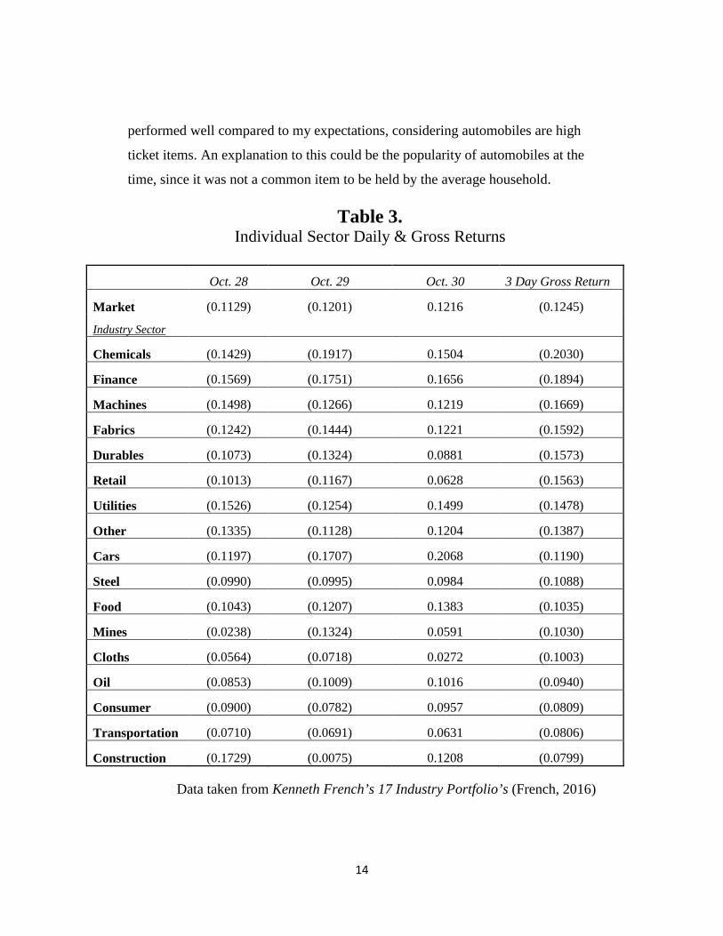
14

performed well compared to my expectations, considering automobiles are high

ticket items. An explanation to this could be the popularity of automobiles at the

time, since it was not a common item to be held by the average household.

Table 3. Individual Sector Daily & Gross Returns

Oct. 28 Oct. 29 Oct. 30 3 Day Gross Return

Market (0.1129) (0.1201) 0.1216 (0.1245)

Industry Sector

Chemicals (0.1429) (0.1917) 0.1504 (0.2030)

Finance (0.1569) (0.1751) 0.1656 (0.1894)

Machines (0.1498) (0.1266) 0.1219 (0.1669)

Fabrics (0.1242) (0.1444) 0.1221 (0.1592)

Durables (0.1073) (0.1324) 0.0881 (0.1573)

Retail (0.1013) (0.1167) 0.0628 (0.1563)

Utilities (0.1526) (0.1254) 0.1499 (0.1478)

Other (0.1335) (0.1128) 0.1204 (0.1387)

Cars (0.1197) (0.1707) 0.2068 (0.1190)

Steel (0.0990) (0.0995) 0.0984 (0.1088)

Food (0.1043) (0.1207) 0.1383 (0.1035)

Mines (0.0238) (0.1324) 0.0591 (0.1030)

Cloths (0.0564) (0.0718) 0.0272 (0.1003)

Oil (0.0853) (0.1009) 0.1016 (0.0940)

Consumer (0.0900) (0.0782) 0.0957 (0.0809)

Transportation (0.0710) (0.0691) 0.0631 (0.0806)

Construction (0.1729) (0.0075) 0.1208 (0.0799)


15

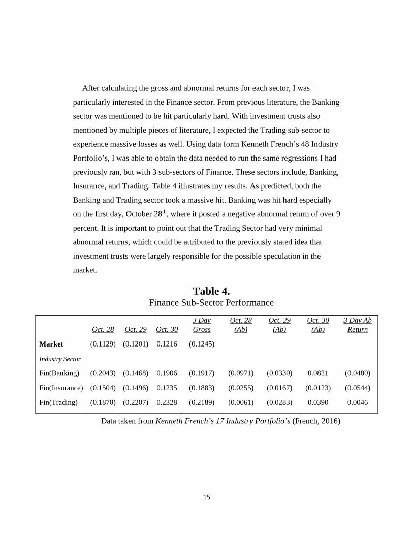
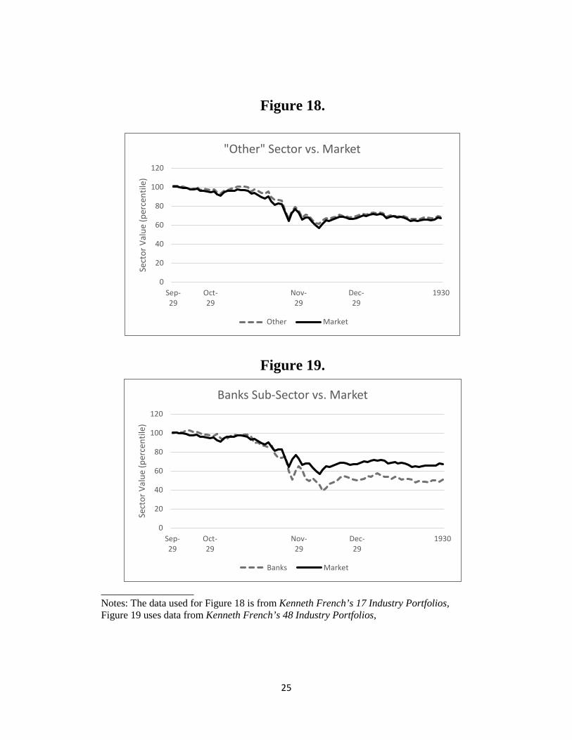
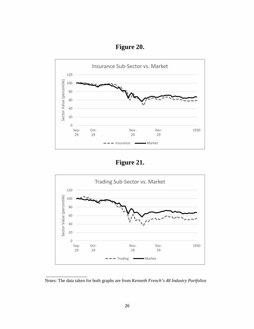
After calculating the gross and abnormal returns for each sector, I was

particularly interested in the Finance sector. From previous literature, the Banking

sector was mentioned to be hit particularly hard. With investment trusts also

mentioned by multiple pieces of literature, I expected the Trading sub-sector to

experience massive losses as well. Using data form Kenneth French’s 48 Industry

Portfolio’s, I was able to obtain the data needed to run the same regressions I had

previously ran, but with 3 sub-sectors of Finance. These sectors include, Banking,

Insurance, and Trading. Table 4 illustrates my results. As predicted, both the

Banking and Trading sector took a massive hit. Banking was hit hard especially

on the first day, October 28th, where it posted a negative abnormal return of over 9

percent. It is important to point out that the Trading Sector had very minimal

abnormal returns, which could be attributed to the previously stated idea that

investment trusts were largely responsible for the possible speculation in the

market.

Table 4. Finance Sub-Sector Performance


Oct. 28 Oct. 29 Oct. 30 3 Day Gross

Oct. 28 (Ab)

Oct. 29 (Ab)

Oct. 30 (Ab)

3 Day Ab Return

Market (0.1129) (0.1201) 0.1216 (0.1245)

Industry Sector

Fin(Banking) (0.2043) (0.1468) 0.1906 (0.1917) (0.0971) (0.0330) 0.0821 (0.0480)

Fin(Insurance) (0.1504) (0.1496) 0.1235 (0.1883) (0.0255) (0.0167) (0.0123) (0.0544)

Fin(Trading) (0.1870) (0.2207) 0.2328 (0.2189) (0.0061) (0.0283) 0.0390 0.0046

16

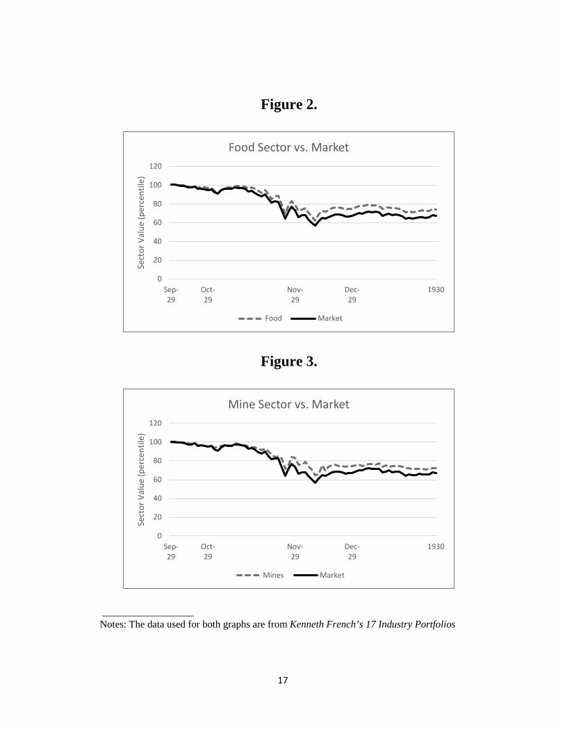
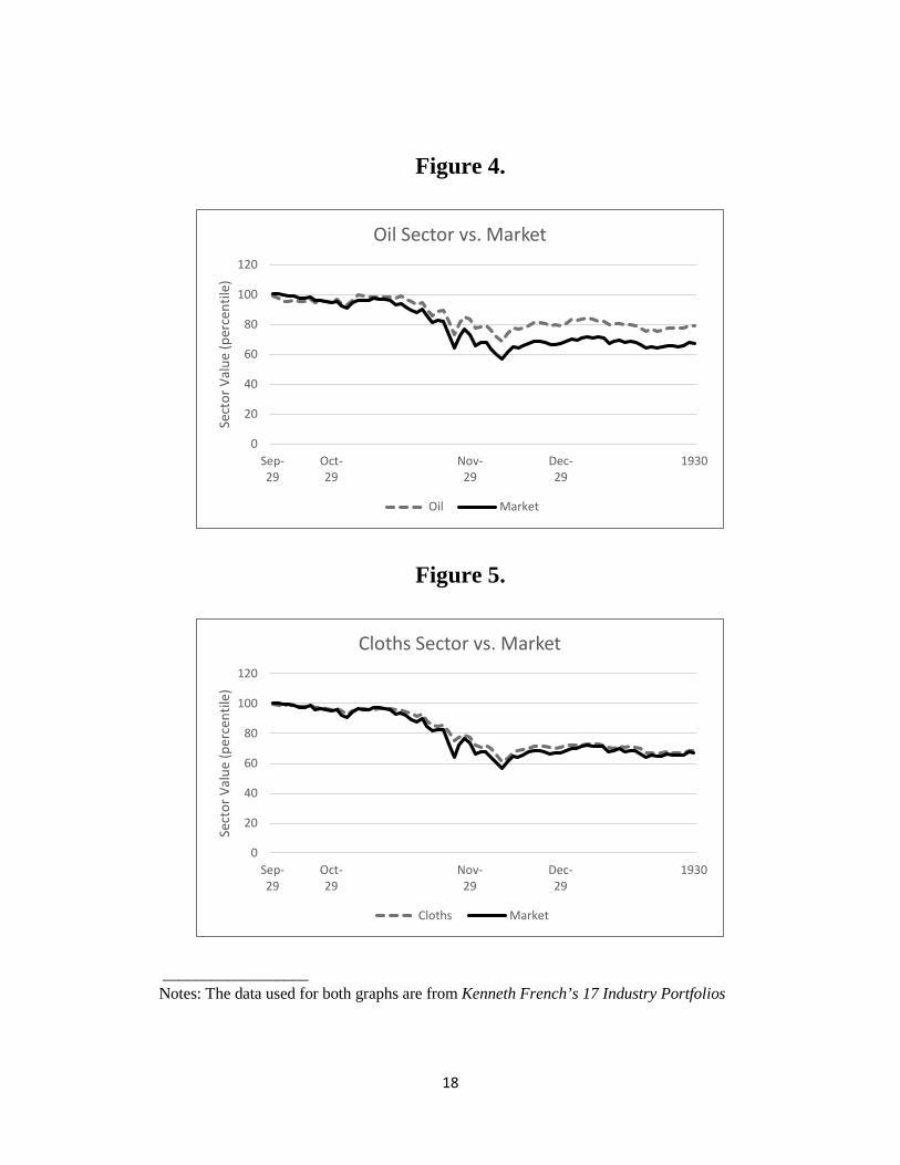
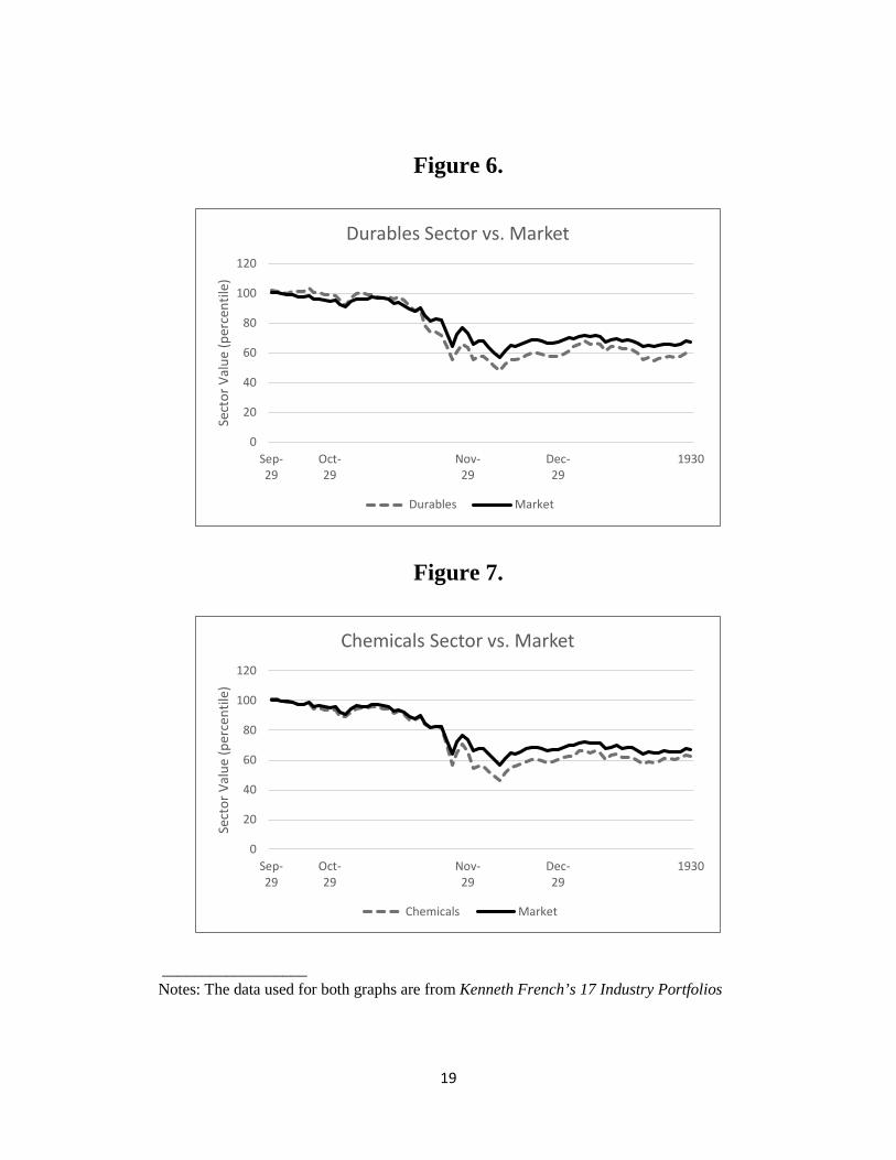
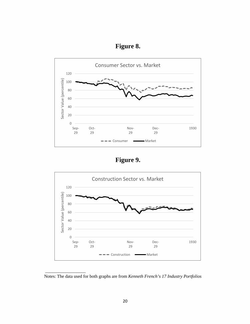
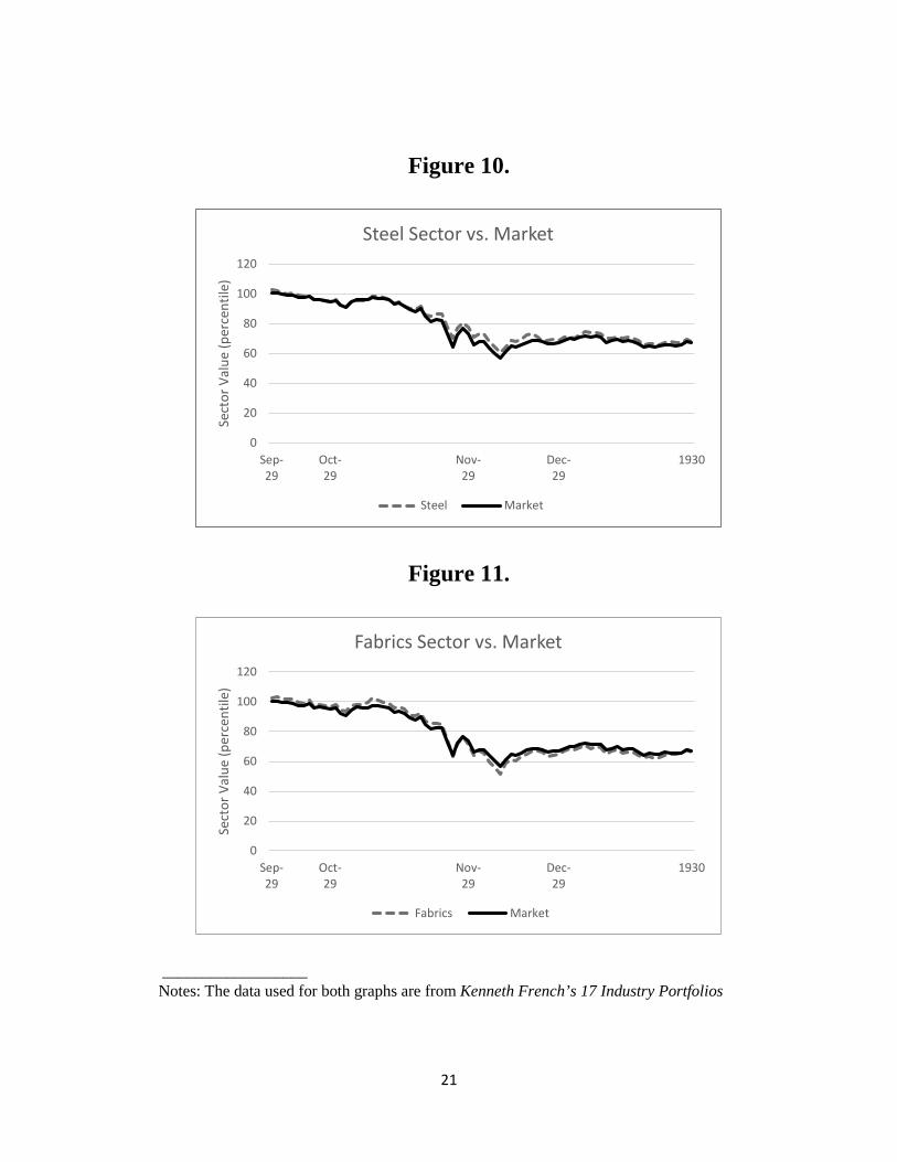
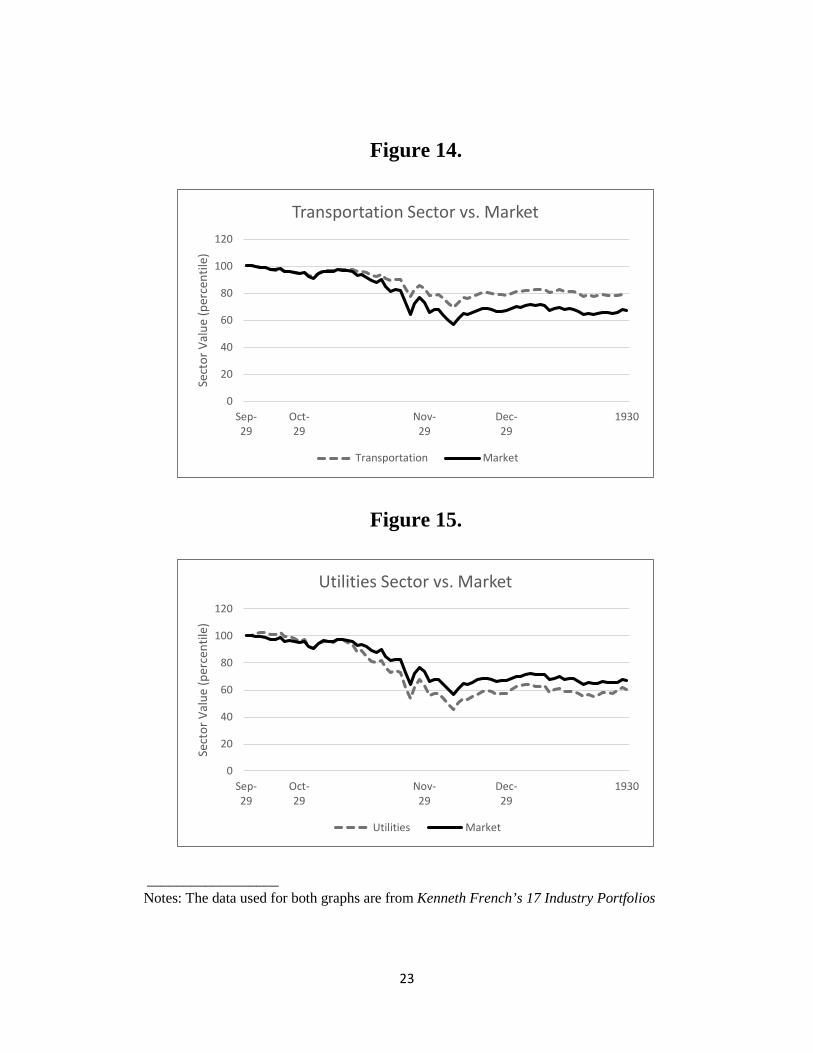
I then created a graph for each industry sector versus the market in terms of

overall gross returns. Each graph starts at the peak of the market, which is in the

middle of September, 1929. The graphs continue until the end of 1929, capturing

the 3 major days of discussion and providing the 1929 year-ending value of each

industry sector. The purpose of these graphs are to compare sector performance

for the 3 days in focus versus the last 2 months of 1929. Particularly interesting is

the year ending performance of the Construction sector versus the Consumer

Goods sector. While both sectors performed relatively well during the 3 major

days of market swings, their year-end performances were drastically different.

Construction performance mimicked the overall market, but Consumer Goods

greatly outperformed. This can probably be explained by the nature of Consumer

Goods being a necessity good that will always have demand from the market. The

Machine sector on the other hand was the 3rd worst performing sector in the crash,

but recovered back towards the average market return by the end of 1929. All

sector comparisons are shown below.

17

Figure 2.

Figure 3.

__________________

Notes: The data used for both graphs are from Kenneth French’s 17 Industry Portfolios

0

20

40

60

80

100

120

Sep-29

Oct-29

Nov-29

Dec-29

1930

Sect

or V

alue

(per

cent

ile)

Food Sector vs. Market

Food Market

0

20

40

60

80

100

120

Sep-29

Oct-29

Nov-29

Dec-29

1930

Sect

or V

alue

(per

cent

ile)

Mine Sector vs. Market

Mines Market

18

Figure 4.

Figure 5.

__________________


0

20

40

60

80

100

120

Sep-29

Oct-29

Nov-29

Dec-29

1930

Sect

or V

alue

(per

cent

ile)

Oil Sector vs. Market

Oil Market

0

20

40

60

80

100

120

Sep-29

Oct-29

Nov-29

Dec-29

1930

Sect

or V

alue

(per

cent

ile)

Cloths Sector vs. Market

Cloths Market

19

Figure 6.

Figure 7.

__________________


0

20

40

60

80

100

120

Sep-29

Oct-29

Nov-29

Dec-29

1930

Sect

or V

alue

(per

cent

ile)

Durables Sector vs. Market

Durables Market

0

20

40

60

80

100

120

Sep-29

Oct-29

Nov-29

Dec-29

1930

Sect

or V

alue

(per

cent

ile)

Chemicals Sector vs. Market

Chemicals Market

20

Figure 8.

Figure 9.

__________________


0

20

40

60

80

100

120

Sep-29

Oct-29

Nov-29

Dec-29

1930

Sect

or V

alue

(per

cent

ile)

Consumer Sector vs. Market

Consumer Market

0

20

40

60

80

100

120

Sep-29

Oct-29

Nov-29

Dec-29

1930

Sect

or V

alue

(per

cent

ile)

Construction Sector vs. Market

Construction Market

21

Figure 10.

Figure 11.

__________________


0

20

40

60

80

100

120

Sep-29

Oct-29

Nov-29

Dec-29

1930

Sect

or V

alue

(per

cent

ile)

Steel Sector vs. Market

Steel Market

0

20

40

60

80

100

120

Sep-29

Oct-29

Nov-29

Dec-29

1930

Sect

or V

alue

(per

cent

ile)

Fabrics Sector vs. Market

Fabrics Market

22

Figure 12.

Figure 13.

__________________


0

20

40

60

80

100

120

Sep-29

Oct-29

Nov-29

Dec-29

1930

Sect

or V

alue

(per

cent

ile)

Machinery Sector vs. Market

Machines Market

0

20

40

60

80

100

120

Sep-29

Oct-29

Nov-29

Dec-29

1930

Sect

or V

alue

(per

cent

ile)

Cars Sector vs. Market

Cars Market

23

Figure 14.

Figure 15.

__________________


0

20

40

60

80

100

120

Sep-29

Oct-29

Nov-29

Dec-29

1930

Sect

or V

alue

(per

cent

ile)

Transportation Sector vs. Market

Transportation Market

0

20

40

60

80

100

120

Sep-29

Oct-29

Nov-29

Dec-29

1930

Sect

or V

alue

(per

cent

ile)

Utilities Sector vs. Market

Utilities Market

24

Figure 16.

Figure 17.

__________________


0

20

40

60

80

100

120

Sep-29

Oct-29

Nov-29

Dec-29

1930

Sect

or V

alue

(per

cent

ile)

Retail Sector vs. Market

Retail Market

0

20

40

60

80

100

120

Sep-29

Oct-29

Nov-29

Dec-29

1930

Sect

or V

alue

(per

cent

ile)

Finance Sector vs. Market

Finance Market

25

Figure 18.

Figure 19.

__________________ Notes: The data used for Figure 18 is from Kenneth French’s 17 Industry Portfolios, Figure 19 uses data from Kenneth French’s 48 Industry Portfolios,

0

20

40

60

80

100

120

Sep-29

Oct-29

Nov-29

Dec-29

1930

Sect

or V

alue

(per

cent

ile)

"Other" Sector vs. Market

Other Market

0

20

40

60

80

100

120

Sep-29

Oct-29

Nov-29

Dec-29

1930

Sect

or V

alue

(per

cent

ile)

Banks Sub-Sector vs. Market

Banks Market

26

Figure 20.

Figure 21.

__________________

Notes: The data taken for both graphs are from Kenneth French’s 48 Industry Portfolios

0

20

40

60

80

100

120

Sep-29

Oct-29

Nov-29

Dec-29

1930

Sect

or V

alue

(per

cent

ile)

Insurance Sub-Sector vs. Market

Insurance Market

0

20

40

60

80

100

120

Sep-29

Oct-29

Nov-29

Dec-29

1930

Sect

or V

alue

(per

cent

ile)

Trading Sub-Sector vs. Market

Trading Market

27

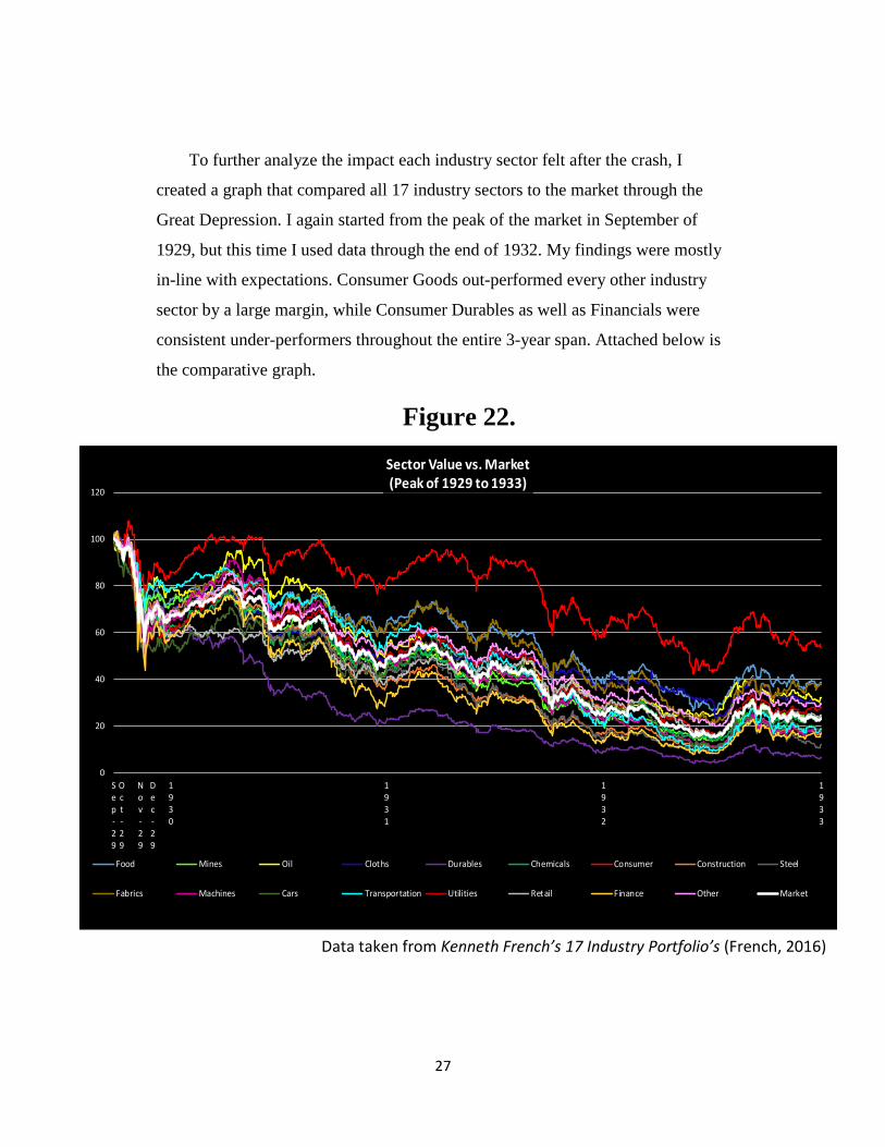
To further analyze the impact each industry sector felt after the crash, I

created a graph that compared all 17 industry sectors to the market through the

Great Depression. I again started from the peak of the market in September of

1929, but this time I used data through the end of 1932. My findings were mostly

in-line with expectations. Consumer Goods out-performed every other industry

sector by a large margin, while Consumer Durables as well as Financials were

consistent under-performers throughout the entire 3-year span. Attached below is

the comparative graph.

Figure 22.

0

20

40

60

80

100

120

Sep-29

Oct-29

Nov-29

Dec-29

1930

1931

1932

1933

Sector Value vs. Market (Peak of 1929 to 1933)

Food Mines Oil Cloths Durables Chemicals Consumer Construction Steel

Fabrics Machines Cars Transportation Utilities Retail Finance Other Market


28

6.) Conclusion

The era of growth and prosperity of the 1920’s ended with the unparalleled

market downfall in the stock market crash of 1929 (Richardson, 2013). With data

previously unavailable, sectoral effects during the crash can now be described

empirically. I formally analyze the effects of the United States Stock Market

Crash on October 28th, 29th, and 30th, 1929, on 17 industry sectors across the

entire market. The market lost over 12.45 percent of its value on those three days,

motivating my research to discover which industry sectors were affected the most.

Using Kenneth French’s 17 Industry’s Portfolio data, I examine daily returns from

the U.S. stock market from 1929 through 1933, allowing me to observe the

sectoral effects from not only the crash, but also the time period of the Great

Depression. I argue that certain industry sectors such as finance, utilities, and

consumer durables would take major hits to their sector value, this is in line with

the work of Galbraith (1954) and Bierman (1998). On the other hand, I argue

industry sectors that encompassed necessities would perform well through the

crash, such as consumer goods and transportation, which is consistent with the

hypothesis of citizen’s loss of purchasing powering in the work of Galbraith

(1954).

In general, my findings are consistent with my arguments above. The main

exception is the Construction sector, which performed abnormally well

throughout the crash. I conclude that the reason for this abnormality was the

sector’s decline in value during the earlier months of 1929, therefore the market’s

correction during the crash had an impact that was not as severe as it was on the

other industry sectors.

29

To further my research, I analyzed 3 specific industry sub-sectors of Finance

industry sector; Banking, Insurance, and Trading. My findings illustrated that the

Banking and Trading sectors took abnormally large hits during the crash, which

was in-line with the research of Bierman (1998). I graphed individual sector

returns versus the market through the end of 1929, as well as all 17 industry

sectors together versus the market through the end of 1932, with the intent to

discover if sector performance during the crash was an indication of future

performance through the Great Depression. My findings proved that industry

sectors generally reverted back to what economic literature would consider as the

typical recession response for that industry.

For future research, the correlation between stock returns by sector to future

industry productions could be examined. Schwert (1990) stated that there is a

strong positive relation between real stock returns and future production rates. By

matching the returns of the sectors I analyzed to industrial data, a study could be

done to see if Schwert’s (1990) theory holds true in the months following the

market crash of 1929, specifically through the Great Depression. Overall, my

findings now allow industry sector returns during the 1929 United States Stock

Market Crash to be empirically described. To the best of my knowledge, no

empirical study has been done to the extent to which I have gone.

30

Works Cited

Bierman, Harold, Jr. The Causes of the 1929 Stock Market Crash. Westport, CT,

Greenwood Press, 1998.

Bierman, Harold, Jr. “The Reasons Stock Crashed in 1929.” Journal of

Investing (1999): 11-18

Bierman, Harold. “The 1929 Stock Market Crash”. EH.Net Encyclopedia, edited

by Robert Whaples. March 26, 2008.

Colombo, Jesse. "Historic Stock Market Crashes, Bubbles & Financial Crises."

The Bubble Bubble. N.p., n.d. Web. 02 Dec. 2016.

Fisher, Irving. The Stock Market Crash and After. New York: Macmillan, 1930.

Galbraith, John Kenneth. The Great Crash of 1929. New York: Houghton Mifflin,

1954.

Hoover, Herbert. The Memoirs of Herbert Hoover. New York, Macmillan, 1952.

Hughes, Patrick. ""The Crash and Early Depression"" "The Crash and Early

Depression"N.p., 1999. Web. 02 Dec. 2016.

French, Kenneth R. "17 Industry Portfolios." Data Library Industry Portfolios. Kenneth

French, 2016. Web.

French, Kenneth R. "48 Industry Portfolios." Data Library Industry Portfolios. Kenneth

French, 2016. Web.

31

Klingaman, William K. 1929: The Year of the Great Crash. New York: Harper &

Row, 1989. Print.

Malkiel, Burton G., A Random Walk Down Wall Street. New York, Norton, 1975

and 1996.

Moggridge, Donald. The Collected Writings of John Maynard Keynes, Volume

XX. New York: Macmillan, 1981.

New York Stock Exchange, Year Book, 1930 – 1931, New York, 1931.

Pettinger, Tejvan. "US Economy of the 1920s." Economics Essays. N.p., 07 May

2007. Web. 02 Dec. 2016.

Richardson, Gary, Alejandro Komai, Michael Gou, and Daniel Park. "Stock

Market Crash of 1929 - A Detailed Essay on an Important Event in the

History of the Federal Reserve." Federal Reserve History. N.p., n.d. Web.

02 Dec. 2016.

Schwert, G. William. "Stock Returns and Real Activity: A Century of Evidence."

The Journal of Finance 45.4 (1990): n. pag. Web.

Senate Committee on Banking and Currency. Stock Exchange Practices.

Washington, 1928.

Sirkin, Gerald, “The Stock Market of 1929 Revisited: A Note,” Business History

Review, Summer 1975, 44, 223-31.

32

Wigmore, Barrie A., The Crash and Its Aftermath. Westport; Greenwood Press,

1985.

White, Eugene N. "The Stock Market Boom and Crash of 1929 Revisited."

Journal of Economic Perspectives 4.2 (1990): 67-83. Web.

Documents

A Sectoral Analysis of the 1929 Stock Market Crash