M. A. FayazbakhshLaboratory for Alternative Energy Conversion,

School of Mechatronic Systems Engineering,

Simon Fraser University,

250-13450 102 Avenue,

Surrey, BC V3T 0A3, Canada

F. BagheriLaboratory for Alternative Energy Conversion,

School of Mechatronic Systems Engineering,

Simon Fraser University,

250-13450 102 Avenue,

Surrey, BC V3T 0A3, Canada

M. Bahrami1Laboratory for Alternative Energy Conversion,

School of Mechatronic Systems Engineering,

Simon Fraser University,

250-13450 102 Avenue,

Surrey, BC V3T 0A3, Canada

e-mail: mbahrami@sfu.ca

A Self-Adjusting Methodfor Real-Time Calculationof Thermal Loads inHVAC-R ApplicationsA significant step in the design of heating, ventilating, air conditioning, and refrigeration(HVAC-R) systems is to calculate room thermal loads. The heating/cooling loads encoun-tered by the room often vary dynamically while the common practice in HVAC-R engi-neering is to calculate the loads for peak conditions and then select the refrigerationsystem accordingly. In this study, a self-adjusting method is proposed for real-time calcu-lation of thermal loads. The method is based on the heat balance method (HBM) and adata-driven approach is followed. Live temperature measurements and a gradientdescent optimization technique are incorporated in the model to adjust the calculationsfor higher accuracy. Using experimental results, it is shown that the proposed methodcan estimate the thermal loads with higher accuracy compared to using sheer physicalproperties of the room in the heat balance calculations, as is often done in design proc-esses. Using the adjusted real-time load estimations in new and existing applications, thesystem performance can be optimized to provide thermal comfort while consuming lessoverall energy. [DOI: 10.1115/1.4031018]

Keywords: HVAC-R, thermal loads, real-time calculation, self-adjusting method, heatbalance method

1 Introduction

A significant portion of the worldwide energy is consumed byHVAC-R systems. The energy consumption by HVAC-R systemsis 50% of the total energy usage in buildings and 20% of the totalnational energy usage in European and American countries [1].HVAC-R energy consumption can exceed 50% of the total energyusage of a building in tropical climates [2]. Furthermore, refriger-ation systems also consume a substantial amount of energy.Supermarket refrigeration systems, as an example, can account forup to 80% of the total energy consumption in the supermarket [3].

Vehicle fuel consumption is also significantly affected by airconditioning. The HVAC-R energy usage in a typical vehicleoutweighs the energy loss to rolling resistance, aerodynamic drag,and driveline losses. HVAC-R systems can reduce the fuel econ-omy of midsized vehicles by more than 20% while increasingNOx and CO emissions by approximately 80% and 70%, respec-tively [4]. Moreover, HVAC-R is a critical system for hybridelectric vehicles and electric vehicles, as it is the second mostenergy consuming system after the electric motor [5]. The energyrequired to provide cabin cooling for thermal comfort can reducethe range of plug-in electric vehicles by up to 50% depending onoutside weather conditions [4]. Less energy consumption bymobile HVAC-R systems directly results in higher mileage andbetter overall efficiency on the road.

Proper design and efficient operation of any HVAC-R systemrequire: (i) accurate calculation of thermal loads and (ii) appropri-ate design and selection of the HVAC-R system. The commonpractice among HVAC-R engineers is to begin by estimating theroom thermal loads. This step consists of a careful study of the

room characteristics such as wall properties, fenestration, open-ings, and air distribution. The room usage pattern, occupancylevel, geographical location, and ambient weather conditions areother necessary data that need to be thoroughly investigatedbefore a decision is made on the design cooling/heating load. AnHVAC-R system that can handle the calculated load is thenselected. As such, much detailed information is required in orderto properly calculate the thermal loads and select the system.Innovative methods that can accurately calculate instantaneousthermal loads without requiring a hefty amount of details can bepromising in the design of new HVAC-R systems.

On–off and modulation controllers are widely used in HVAC-Rsystems, which use the room temperature as the controlled vari-able [6]. However, such controllers mostly act upon the currenttemperature value and are not aware of the actual thermal loadand its variation pattern over the duty cycle. It is shown that intel-ligent control of the HVAC-R operation based on thermal loadprediction can help maintain air quality while minimizing energyconsumption [7,8]. By predicting the thermal loads in real-time,controllers are enabled to not only provide thermal comfort in thecurrent condition but also adjust the system operation to cope withupcoming conditions in an efficient manner. Having real-timeestimation of thermal loads can result in improved energy effi-ciency, as the HVAC-R system is enabled to adapt to variousdemand situations. Arguello-Serrano and Velez-Reyes [9] statedthat availability of thermal load estimations efficiently allows theHVAC-R controller to provide comfort regardless of the thermalloads. Afram and Janabi-Sharifi [10] showed that improved loadestimations can lead to the design and testing of more advancedcontrollers. Zhu et al. [11] studied an optimal control strategy forminimizing the energy consumption using variable refrigerantflow and variable air volume air conditioning systems. Qureshiand Tassou [12] reviewed various methods of capacity controlin refrigeration systems and stated that using variable-speedcompressors can be the most energy-efficient method for capacity

1Corresponding author.Contributed by the Heat Transfer Division of ASME for publication in the

JOURNAL OF THERMAL SCIENCE AND ENGINEERING APPLICATIONS. Manuscript receivedMarch 20, 2015; final manuscript received June 8, 2015; published online July 28,2015. Assoc. Editor: Zahid Ayub.

Journal of Thermal Science and Engineering Applications DECEMBER 2015, Vol. 7 / 041012-1Copyright VC 2015 by ASME

Downloaded From: http://thermalscienceapplication.asmedigitalcollection.asme.org/ on 01/09/2018 Terms of Use: http://www.asme.org/about-asme/terms-of-use

control. Therefore, the ability to accurately predict thermal loadsin real-time can improve the feedback information for the controlof HVAC-R systems, which in turn results in significant reductionof total energy consumption and greenhouse gas emissions.

The literature is rich with various approaches proposed forcalculation of thermal loads. The American Society of Heating,Refrigerating, and Air Conditioning Engineers (ASHRAE)recognize some of them including the HBM [13]. HBM is astraightforward and rigorous method that involves calculating asurface-by-surface heat balance of the surrounding walls of theroom through consideration of conductive, convective, and radia-tive heat transfer mechanisms. After calculation of heat flowsacross all walls and openings, the heat balance equation is solvedfor the room air to complete the solution procedure. The methodhas been extensively used in residential, nonresidential, andmobile applications [14–17].

HBM is known as a “forward” or “law-driven” approach, i.e.,it estimates the loads based on rigorous details of the room.Feedback data from the system are seldom incorporated in theformulations of this method. In contrast to HBM, “inverse” or“data-driven” methods study existing HVAC-R systems and allowthe thermal performance of the system to be inferred frommeasured temperature values. Such approaches mathematicallyevaluate the loads through learning and testing rather than analyz-ing the heat transfer equations. Li et al. [18] presented four model-ing techniques for hourly prediction of thermal loads. Themethods included back propagation neural network, radial basisfunction neural network, general regression neural network, andsupport vector machine. The mathematical models they used cor-related the cooling load with parameters such as the ambientweather, but the heat transfer equations were not explicitly used.Kashiwagi and Tobi [19] also proposed a neural network algo-rithm for prediction of thermal loads. Ben-Nakhi and Mahmoud[20] used general regression neural networks and concluded that aproperly designed neural network is a powerful tool for optimiz-ing thermal energy storage in buildings based only on externaltemperature records. They claimed that their set of algorithmscould learn over time and improve the prediction ability. Sousaet al. [21] developed a fuzzy controller to be incorporated as a pre-dictor in a nonlinear model-based predictive controller. Yao et al.[22] used a case study to show that a combined forecasting modelbased on a combination of neural networks and a few othermethods can be promising for predicting a building’s hourly loadfor the future hours. Solmaz et al. [23] used the same concept ofneural networks to predict the hourly cooling load for vehicle cab-ins. Fayazbakhsh et al. [24] proposed a simple method that canestimate the total heat gain and thermal inertia of the room usingan inverse calculation method and real-time temperaturemeasurements.

Although producing acceptable results, methods that are purelybased on artificial intelligence are inherently unaware of the heattransfer mechanisms. Thus, they might prove unreliable in new

scenarios and conditions for which they are not trained. A numberof recent studies aim at combining artificial intelligence algo-rithms with conventional load calculation methods to improvethem. For instance, Wang and Xu [25,26] used genetic algorithmto estimate thermal parameters of a building thermal networkmodel using the operation data collected from site monitoring.They combined a resistance–capacitance (RC) model of the build-ing envelope with a data-driven approach where their RC modelparameters were corrected via real-time measurements. Theresults of conventional load calculation methods can be improvedby incorporating new mathematical algorithms that act on simplereal-time measurements.

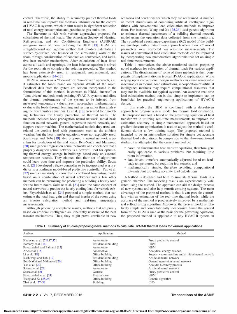
Table 1 summarizes the above-mentioned studies proposingnovel methods for calculation of thermal loads for various appli-cations. The disadvantage of some of these methods is their com-plexity of implementation in typical HVAC-R applications. Whilerelying upon conventional design methods can cause remarkableinaccuracies in thermal load estimations, incorporation of artificialintelligence methods may require computational resources thatmay not be available for typical systems. An accurate real-timeload calculation method that is also simple to implement can bebeneficial for practical engineering applications of HVAC-Rdesign.

In this study, the HBM is combined with a data-drivenapproach to propose a new model for thermal load estimation.The proposed method is based on the governing equations of heattransfer while utilizing real-time measurements to improve theestimation accuracy. A simple mathematical approach based ongradient descent optimization is used to adjust the method’s coef-ficients during a few training steps. The proposed method isintended to be an intermediate solution for simple yet accuratethermal load calculations. In comparison to the above-mentionedstudies, it is attempted that the current method be:

• based on fundamental heat transfer equations, therefore gen-erally applicable to various problems, but requiring littleroom information,

• data-driven, therefore automatically adjusted based on feed-back temperatures, but requiring few sensors, and

• mathematically simple, therefore avoiding computationalintensity, but providing accurate load calculations.

A testbed is designed and built to simulate thermal loads in ageneric chamber. The modeling results are experimentally vali-dated using the testbed. The approach can aid the design processof new systems and also help retrofit existing systems. The mainadvantage of the proposed method is that it can provide control-lers with an estimation of the real-time thermal loads, while theaccuracy of the method is progressively improved by a mathemat-ical self-adjusting algorithm. Moreover, the present model is rela-tively simple and computationally inexpensive. Since the generalform of the HBM is used as the basis for the governing equations,the proposed method is applicable to any HVAC-R system in

Table 1 Summary of studies proposing novel methods to calculate HVAC-R thermal loads for various applications

Authors Application Method

Khayyam et al. [7,8,17,37] Automotive Fuzzy predictive controlBarnaby et al. [14] Residential building HBMFayazbakhsh and Bahrami [15] Automotive HBMArici et al. [16] Automotive Analytical energy balanceLi et al. [18] Office building Support vector machine and artificial neural networkKashiwagi and Tobi [19] Residential building Artificial neural networkBen-Nakhi and Mahmoud [20] Office building General regression neural networkYao et al. [22] Office building Analytic hierarchy processSolmaz et al. [23] Automotive Artificial neural networkSousa et al. [21] Generic Fuzzy predictive controlFayazbakhsh et al. [24] Freezer room HBMWang and Xu [25,26] Office building Genetic algorithmZhai et al. [27–32] Building CFD

041012-2 / Vol. 7, DECEMBER 2015 Transactions of the ASME

Downloaded From: http://thermalscienceapplication.asmedigitalcollection.asme.org/ on 01/09/2018 Terms of Use: http://www.asme.org/about-asme/terms-of-use

general. As such, the same concept can be used for residentialbuildings, office buildings, freezer rooms, and vehicle air condi-tioning systems.

2 Model Development

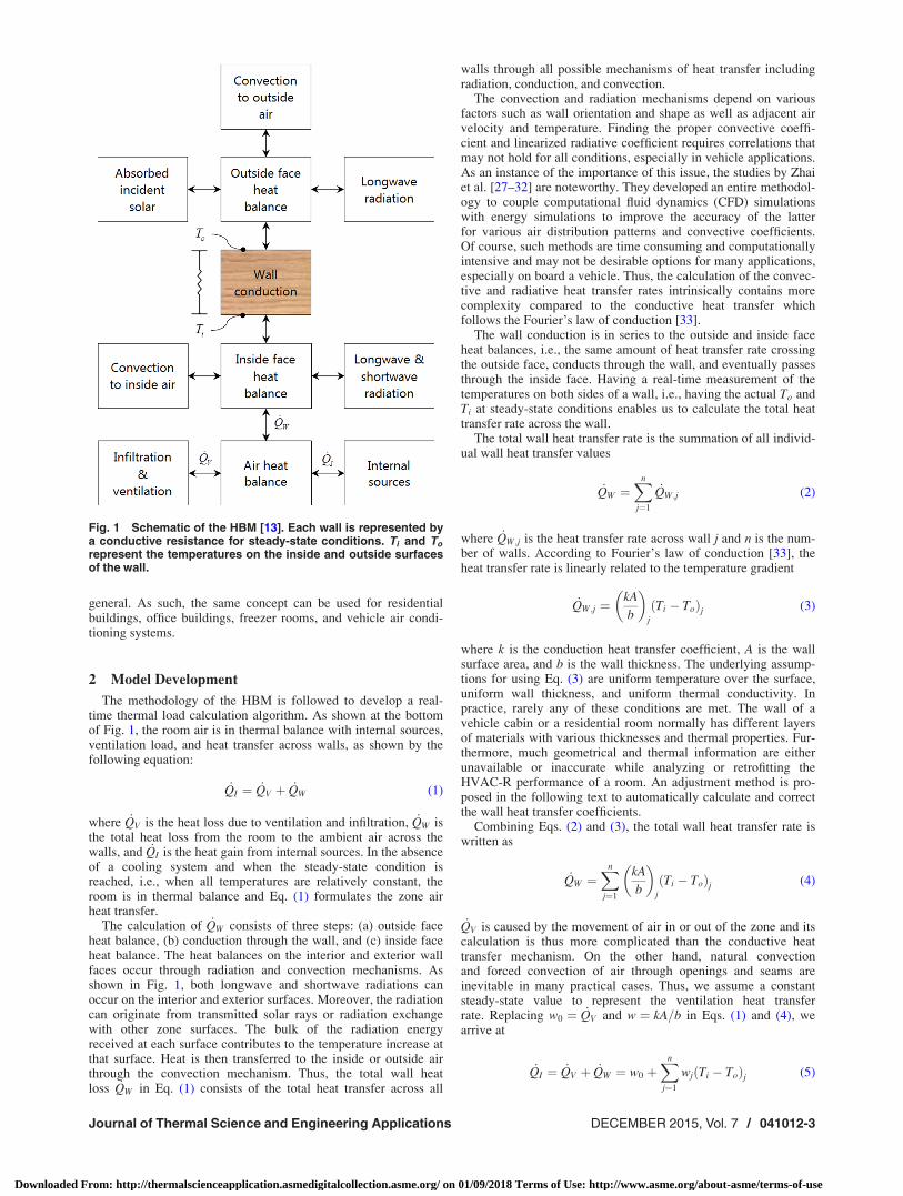
The methodology of the HBM is followed to develop a real-time thermal load calculation algorithm. As shown at the bottomof Fig. 1, the room air is in thermal balance with internal sources,ventilation load, and heat transfer across walls, as shown by thefollowing equation:

_QI ¼ _QV þ _QW (1)

where _QV is the heat loss due to ventilation and infiltration, _QW isthe total heat loss from the room to the ambient air across thewalls, and _QI is the heat gain from internal sources. In the absenceof a cooling system and when the steady-state condition isreached, i.e., when all temperatures are relatively constant, theroom is in thermal balance and Eq. (1) formulates the zone airheat transfer.

The calculation of _QW consists of three steps: (a) outside faceheat balance, (b) conduction through the wall, and (c) inside faceheat balance. The heat balances on the interior and exterior wallfaces occur through radiation and convection mechanisms. Asshown in Fig. 1, both longwave and shortwave radiations canoccur on the interior and exterior surfaces. Moreover, the radiationcan originate from transmitted solar rays or radiation exchangewith other zone surfaces. The bulk of the radiation energyreceived at each surface contributes to the temperature increase atthat surface. Heat is then transferred to the inside or outside airthrough the convection mechanism. Thus, the total wall heatloss _QW in Eq. (1) consists of the total heat transfer across all

walls through all possible mechanisms of heat transfer includingradiation, conduction, and convection.

The convection and radiation mechanisms depend on variousfactors such as wall orientation and shape as well as adjacent airvelocity and temperature. Finding the proper convective coeffi-cient and linearized radiative coefficient requires correlations thatmay not hold for all conditions, especially in vehicle applications.As an instance of the importance of this issue, the studies by Zhaiet al. [27–32] are noteworthy. They developed an entire methodol-ogy to couple computational fluid dynamics (CFD) simulationswith energy simulations to improve the accuracy of the latterfor various air distribution patterns and convective coefficients.Of course, such methods are time consuming and computationallyintensive and may not be desirable options for many applications,especially on board a vehicle. Thus, the calculation of the convec-tive and radiative heat transfer rates intrinsically contains morecomplexity compared to the conductive heat transfer whichfollows the Fourier’s law of conduction [33].

The wall conduction is in series to the outside and inside faceheat balances, i.e., the same amount of heat transfer rate crossingthe outside face, conducts through the wall, and eventually passesthrough the inside face. Having a real-time measurement of thetemperatures on both sides of a wall, i.e., having the actual To andTi at steady-state conditions enables us to calculate the total heattransfer rate across the wall.

The total wall heat transfer rate is the summation of all individ-ual wall heat transfer values

_QW ¼Xn

j¼1

_QW;j (2)

where _QW;j is the heat transfer rate across wall j and n is the num-ber of walls. According to Fourier’s law of conduction [33], theheat transfer rate is linearly related to the temperature gradient

_QW;j ¼kA

b

� �j

Ti � Toð Þj (3)

where k is the conduction heat transfer coefficient, A is the wallsurface area, and b is the wall thickness. The underlying assump-tions for using Eq. (3) are uniform temperature over the surface,uniform wall thickness, and uniform thermal conductivity. Inpractice, rarely any of these conditions are met. The wall of avehicle cabin or a residential room normally has different layersof materials with various thicknesses and thermal properties. Fur-thermore, much geometrical and thermal information are eitherunavailable or inaccurate while analyzing or retrofitting theHVAC-R performance of a room. An adjustment method is pro-posed in the following text to automatically calculate and correctthe wall heat transfer coefficients.

Combining Eqs. (2) and (3), the total wall heat transfer rate iswritten as

_QW ¼Xn

j¼1

kA

b

� �j

Ti � Toð Þj (4)

_QV is caused by the movement of air in or out of the zone and itscalculation is thus more complicated than the conductive heattransfer mechanism. On the other hand, natural convectionand forced convection of air through openings and seams areinevitable in many practical cases. Thus, we assume a constantsteady-state value to represent the ventilation heat transferrate. Replacing w0 ¼ _QV and w ¼ kA=b in Eqs. (1) and (4), wearrive at

_QI ¼ _QV þ _QW ¼ w0 þXn

j¼1

wj Ti � Toð Þj (5)

Fig. 1 Schematic of the HBM [13]. Each wall is represented bya conductive resistance for steady-state conditions. Ti and To

represent the temperatures on the inside and outside surfacesof the wall.

Journal of Thermal Science and Engineering Applications DECEMBER 2015, Vol. 7 / 041012-3

Downloaded From: http://thermalscienceapplication.asmedigitalcollection.asme.org/ on 01/09/2018 Terms of Use: http://www.asme.org/about-asme/terms-of-use

where w0 – wn are called the weight factors. As previouslymentioned, there are always uncertainties and inaccuraciesassociated with the calculation of the weight factors. Nevertheless,considering Eq. (1) for steady-state conditions, if _QI and the tem-peratures Ti and To are known for a few cases, a gradient descentoptimization technique can be utilized to adjust the weight factorsprogressively and use the adjusted weights for future load calcula-tions. This approach leads to a self-adjusting algorithm for thereal-time calculation of the wall heat transfer rates.

Equation (5) is a linear function in which w0 is called the “biasweight” and w1 – wn are called the “input weights” [22,34–36]. Inorder to establish a simple formula for updating the weight fac-tors, a “transfer function” f can be applied to the right-hand sideof Eq. (5) to arrive at the following:

O ¼ f w0 þXn

j¼1

wj Ti � Toð Þj

!(6)

where O is the calculated output and f is the sigmoidfunction [36]

f xð Þ ¼ 1

1þ exp �xð Þ (7)

Finally, in order to adjust the weight factors w0 – wn, a trainingprocess is required where _QI is known alongside the measuredtemperatures Ti and To for a few cases. The correction procedureis implemented according to [34]

wmþ1j ¼ wm

j þ g D� Oð Þm Ti � Toð Þmj (8)

where g is the learning rate. D ¼ f _QI

� �is the desired output found

from the known _QI values of the training phase and m denotes thestep number of the training algorithm. The set of weight factorsfound by the training algorithm is eventually inserted in Eq. (5) toarrive at the real-time thermal load for future cases where thedirect heat gain from internal sources is unknown. Note that theoriginal equation of heat balance in Eq. (1) is written for steady-state conditions. As such, the training scheme of Eq. (8) is mostreliably applicable to temperature measurements at steady-stateconditions. In practice, once the steady-state condition is reached,the temperatures are sensed at every time step, say every second,and the training procedure is performed using those readings.However, although the mentioned steps occur in time, they aremerely regarded as iteration steps for Eq. (8). Therefore, the over-all algorithm must not be mistaken for a transient formulation.

In summary, the objective function of the discussed optimiza-tion algorithm is F ¼ D� Oj j, which is the difference betweenthe real internal heat gain and the calculated internal heat gain.Although the weight factors may mathematically converge tonegative values, it is necessary that they retain their physicalmeaning, i.e., the wall thermal conductance values, which arealways positive. Thus, it is deemed to minimize the objectivefunction F subject to the constraints w0;w1;…;wn > 0. A signifi-cant advantage of the proposed technique is that considerably lit-tle information need to be known about the room in order tocalculate the thermal loads. The weight factors which are updatedin the training procedure can be initiated from any arbitrary valuesuch as zero.

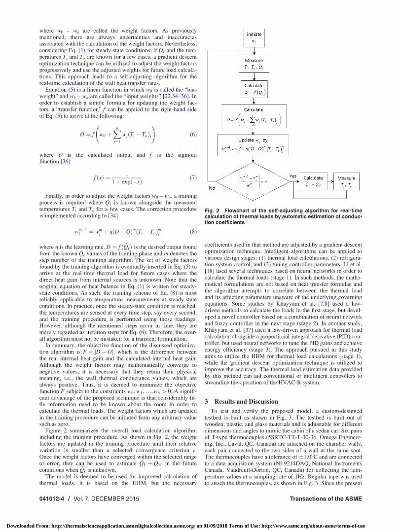
Figure 2 summarizes the overall load calculation algorithmincluding the training procedure. As shown in Fig. 2, the weightfactors are updated in the training procedure until their relativevariation is smaller than a selected convergence criterion e.Once the weight factors have converged within the selected rangeof error, they can be used to estimate _QV þ _QW in the futureconditions when _QI is unknown.

The model is deemed to be used for improved calculation ofthermal loads. It is based on the HBM, but the necessary

coefficients used in that method are adjusted by a gradient descentoptimization technique. Intelligent algorithms can be applied tovarious design stages: (1) thermal load calculations, (2) refrigera-tion system control, and (3) tuning controller parameters. Li et al.[18] used several techniques based on neural networks in order tocalculate the thermal loads (stage 1). In such methods, the mathe-matical formulations are not based on heat transfer formulae andthe algorithm attempts to correlate between the thermal loadand its affecting parameters unaware of the underlying governingequations. Some studies by Khayyam et al. [7,8] used a law-driven methods to calculate the loads in the first stage, but devel-oped a novel controller based on a combination of neural networkand fuzzy controller in the next stage (stage 2). In another study,Khayyam et al. [37] used a law-driven approach for thermal loadcalculation alongside a proportional-integral-derivative (PID) con-troller, but used neural networks to tune the PID gains and achieveenergy efficiency (stage 3). The approach pursued in this studyaims to utilize the HBM for thermal load calculations (stage 1),while the gradient descent optimization technique is utilized toimprove the accuracy. The thermal load estimation data providedby this method can aid conventional or intelligent controllers tostreamline the operation of the HVAC-R system.

3 Results and Discussion

To test and verify the proposed model, a custom-designedtestbed is built as shown in Fig. 3. The testbed is built out ofwooden, plastic, and glass materials and is adjustable for differentdimensions and angles to mimic the cabin of a sedan car. Six pairsof T-type thermocouples (5SRTC-TT-T-30-36, Omega Engineer-ing, Inc., Laval, QC, Canada) are attached on the chamber walls,each pair connected to the two sides of a wall at the same spot.The thermocouples have a tolerance of 61:0�C and are connectedto a data acquisition system (NI 9214DAQ, National InstrumentsCanada, Vaudreuil-Dorion, QC, Canada) for collecting the tem-perature values at a sampling rate of 1Hz. Regular tape was usedto attach the thermocouples, as shown in Fig. 3. Since the present

Fig. 2 Flowchart of the self-adjusting algorithm for real-timecalculation of thermal loads by automatic estimation of conduc-tion coefficients

041012-4 / Vol. 7, DECEMBER 2015 Transactions of the ASME

Downloaded From: http://thermalscienceapplication.asmedigitalcollection.asme.org/ on 01/09/2018 Terms of Use: http://www.asme.org/about-asme/terms-of-use

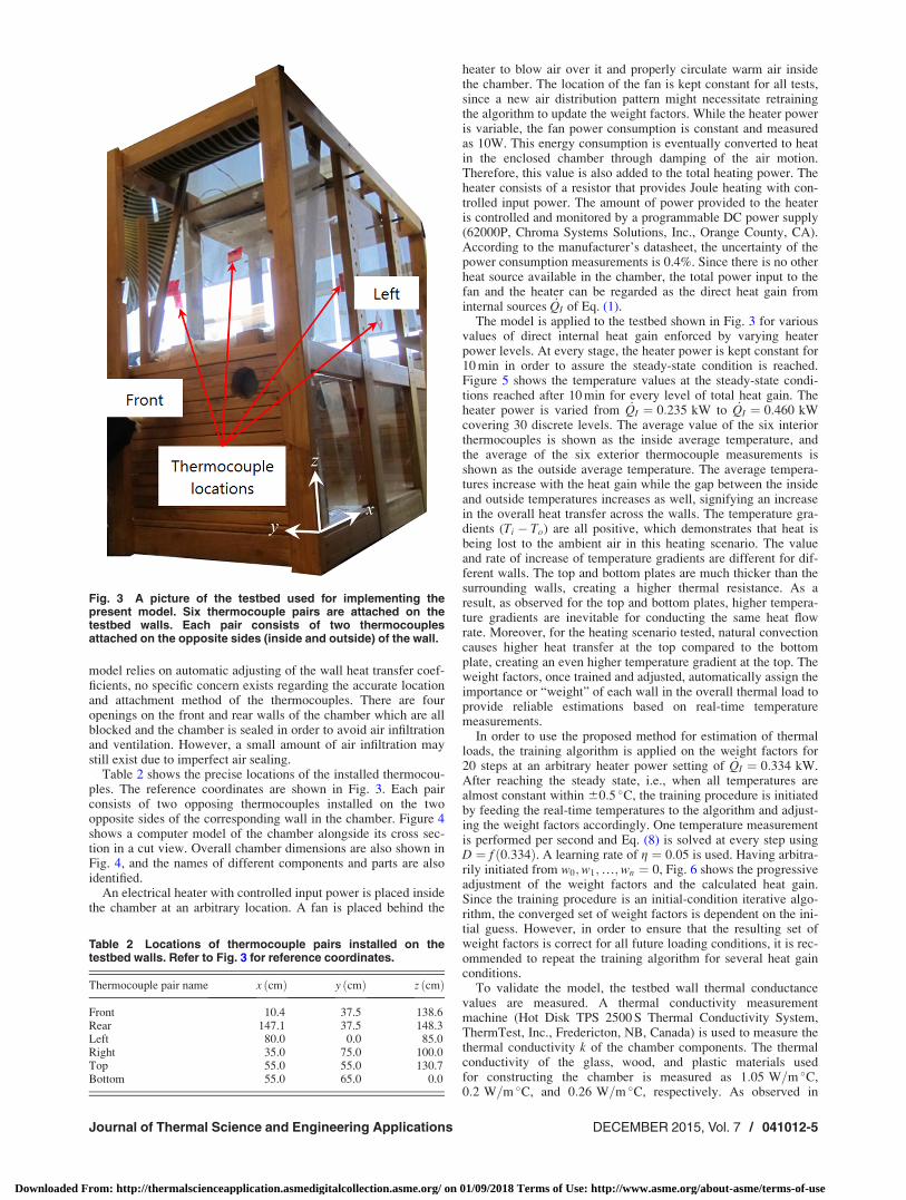
model relies on automatic adjusting of the wall heat transfer coef-ficients, no specific concern exists regarding the accurate locationand attachment method of the thermocouples. There are fouropenings on the front and rear walls of the chamber which are allblocked and the chamber is sealed in order to avoid air infiltrationand ventilation. However, a small amount of air infiltration maystill exist due to imperfect air sealing.

Table 2 shows the precise locations of the installed thermocou-ples. The reference coordinates are shown in Fig. 3. Each pairconsists of two opposing thermocouples installed on the twoopposite sides of the corresponding wall in the chamber. Figure 4shows a computer model of the chamber alongside its cross sec-tion in a cut view. Overall chamber dimensions are also shown inFig. 4, and the names of different components and parts are alsoidentified.

An electrical heater with controlled input power is placed insidethe chamber at an arbitrary location. A fan is placed behind the

heater to blow air over it and properly circulate warm air insidethe chamber. The location of the fan is kept constant for all tests,since a new air distribution pattern might necessitate retrainingthe algorithm to update the weight factors. While the heater poweris variable, the fan power consumption is constant and measuredas 10W. This energy consumption is eventually converted to heatin the enclosed chamber through damping of the air motion.Therefore, this value is also added to the total heating power. Theheater consists of a resistor that provides Joule heating with con-trolled input power. The amount of power provided to the heateris controlled and monitored by a programmable DC power supply(62000P, Chroma Systems Solutions, Inc., Orange County, CA).According to the manufacturer’s datasheet, the uncertainty of thepower consumption measurements is 0.4%. Since there is no otherheat source available in the chamber, the total power input to thefan and the heater can be regarded as the direct heat gain frominternal sources _QI of Eq. (1).

The model is applied to the testbed shown in Fig. 3 for variousvalues of direct internal heat gain enforced by varying heaterpower levels. At every stage, the heater power is kept constant for10 min in order to assure the steady-state condition is reached.Figure 5 shows the temperature values at the steady-state condi-tions reached after 10 min for every level of total heat gain. Theheater power is varied from _QI ¼ 0:235 kW to _QI ¼ 0:460 kWcovering 30 discrete levels. The average value of the six interiorthermocouples is shown as the inside average temperature, andthe average of the six exterior thermocouple measurements isshown as the outside average temperature. The average tempera-tures increase with the heat gain while the gap between the insideand outside temperatures increases as well, signifying an increasein the overall heat transfer across the walls. The temperature gra-dients (Ti � To) are all positive, which demonstrates that heat isbeing lost to the ambient air in this heating scenario. The valueand rate of increase of temperature gradients are different for dif-ferent walls. The top and bottom plates are much thicker than thesurrounding walls, creating a higher thermal resistance. As aresult, as observed for the top and bottom plates, higher tempera-ture gradients are inevitable for conducting the same heat flowrate. Moreover, for the heating scenario tested, natural convectioncauses higher heat transfer at the top compared to the bottomplate, creating an even higher temperature gradient at the top. Theweight factors, once trained and adjusted, automatically assign theimportance or “weight” of each wall in the overall thermal load toprovide reliable estimations based on real-time temperaturemeasurements.

In order to use the proposed method for estimation of thermalloads, the training algorithm is applied on the weight factors for20 steps at an arbitrary heater power setting of _QI ¼ 0:334 kW.After reaching the steady state, i.e., when all temperatures arealmost constant within 60:5 �C, the training procedure is initiatedby feeding the real-time temperatures to the algorithm and adjust-ing the weight factors accordingly. One temperature measurementis performed per second and Eq. (8) is solved at every step usingD ¼ f 0:334ð Þ. A learning rate of g ¼ 0:05 is used. Having arbitra-rily initiated from w0;w1;…;wn ¼ 0, Fig. 6 shows the progressiveadjustment of the weight factors and the calculated heat gain.Since the training procedure is an initial-condition iterative algo-rithm, the converged set of weight factors is dependent on the ini-tial guess. However, in order to ensure that the resulting set ofweight factors is correct for all future loading conditions, it is rec-ommended to repeat the training algorithm for several heat gainconditions.

To validate the model, the testbed wall thermal conductancevalues are measured. A thermal conductivity measurementmachine (Hot Disk TPS 2500 S Thermal Conductivity System,ThermTest, Inc., Fredericton, NB, Canada) is used to measure thethermal conductivity k of the chamber components. The thermalconductivity of the glass, wood, and plastic materials usedfor constructing the chamber is measured as 1:05 W=m �C,0:2 W=m �C, and 0:26 W=m �C, respectively. As observed in

Fig. 3 A picture of the testbed used for implementing thepresent model. Six thermocouple pairs are attached on thetestbed walls. Each pair consists of two thermocouplesattached on the opposite sides (inside and outside) of the wall.

Table 2 Locations of thermocouple pairs installed on thetestbed walls. Refer to Fig. 3 for reference coordinates.

Thermocouple pair name x cmð Þ y cmð Þ z cmð Þ

Front 10.4 37.5 138.6Rear 147.1 37.5 148.3Left 80.0 0.0 85.0Right 35.0 75.0 100.0Top 55.0 55.0 130.7Bottom 55.0 65.0 0.0

Journal of Thermal Science and Engineering Applications DECEMBER 2015, Vol. 7 / 041012-5

Downloaded From: http://thermalscienceapplication.asmedigitalcollection.asme.org/ on 01/09/2018 Terms of Use: http://www.asme.org/about-asme/terms-of-use

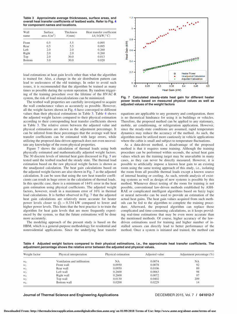
Fig. 3, the chamber walls do not consist of uniform materials.Furthermore, the wall shapes are not necessarily flat and theirthicknesses are nonuniform. Table 3 shows an approximate aver-age of the thicknesses, surface areas, and overall heat transfercoefficients of the testbed walls.

In common engineering practice, the designer would investigatethe room and find the conductance values shown in Table 3 to beused in the HBM and Eq. (4). If the conductance values foundfrom the careful measurement of thickness, area, and conductivityare precise, they will satisfy the heat balance equation and accu-rate load calculations will follow. However, accurate materialdata are seldom available to be used in precise estimations of con-ductance values. Furthermore, wall materials and insulations areoften subject to degradation, which changes their conductivityvalue. Moreover, the averaging and approximation of the proper-ties by the engineer are prone to inaccuracies that can result inthermal load miscalculations. The current method provides ameans to overcome these issues by utilizing actual system data forcalculation adjustment. The proposed method can thus be

specifically promising for retrofitting existing systems and design-ing new ones.

Table 4 shows the adjusted weight factors after 20 correctionsteps shown in Fig. 6. Note that all the weight factors are initiatedfrom zero, which means that the method can perform well almostunsupervised. As observed in Fig. 6, the calculated power is con-verged to the exact heater power in seven steps, i.e., after only 7 sof training. It shows that a controller designed based on the pro-posed algorithm can adjust to the room conditions within secondsof the training procedure initiation.

Since the gradient descent optimization technique inherentlyfinds the local minima of the objective function [38], the adjustedweight factors depend on their initial values and can converge to acombination of w0 – w6 that may not necessarily correspond tothe global minimum of the objective function. As such, a disad-vantage of the proposed method is that the weight factors mayconverge to wrong values and the training algorithm can gettrapped in local minima. Bad convergence may result in incorrect

Fig. 4 Computer model of the testbed showing its overall dimensions and components: (a)full chamber model and (b) cut view showing the chamber’s cross section

Fig. 5 Average inside and outside temperatures (left axis) andtemperature difference between inside and outside wall surfa-ces (Ti � To) (right axis) for various levels of controlled internalheat gain in the testbed

Fig. 6 Progressive training of weight factors and calculatedheat gain for an arbitrary heat gain of _QI 5 0:334 kW. The weightfactors are adjusted based on real-time temperature measure-ments and the known heat gain.

041012-6 / Vol. 7, DECEMBER 2015 Transactions of the ASME

Downloaded From: http://thermalscienceapplication.asmedigitalcollection.asme.org/ on 01/09/2018 Terms of Use: http://www.asme.org/about-asme/terms-of-use

load estimations at heat gain levels other than what the algorithmis trained for. Also, a change in the air distribution pattern canlead to uselessness of the old trainings. In order to avoid suchissues, it is recommended that the algorithm be trained as manytimes as possible during the system operation. By random trigger-ing of the training procedure over the lifetime of the HVAC-Rsystem, the risk of load miscalculations can be minimized.

The testbed wall properties are carefully investigated to acquirethe wall conductance values as accurately as possible. However,all the weight factors shown in Fig. 6 have converged to differentvalues than their physical estimations in Table 3. Table 4 showsthe adjusted weight factors compared to their physical estimationaccording to their corresponding heat transfer coefficients shownin Table 3. The relative errors between the adjusted value andphysical estimations are shown as the adjustment percentage. Itcan be inferred from these percentages that the average wall heattransfer coefficients can be estimated with large errors, whileutilizing the proposed data-driven approach does not even necessi-tate any knowledge of the room physical properties.

Figure 7 shows the calculation of thermal loads using bothphysically estimated and mathematically adjusted weight factors.The 30 discrete levels of internal heat gain discussed in Fig. 5 aretested until the testbed reached the steady state. The thermal loadestimation based on the raw physical weight factors is shown asthe unadjusted calculation. The heat gain calculations based onthe adjusted weight factors are also shown in Fig. 7 as the adjustedcalculation. It can be seen that using the raw heat transfer coeffi-cients can result in huge errors in the calculation of thermal loads.In this specific case, there is a minimum of 144% error in the heatgain estimation using physical coefficients. The adjusted weightfactors, however, result in a maximum error of 16% in thermalload calculations. It is further observed in Fig. 7 that the adjustedheat gain calculations are relatively more accurate for heaterpower levels closer to _QI ¼ 0:334 kW compared to lower andhigher power levels. This hints that the best practice is to train thealgorithm for heat gain levels that are more frequently experi-enced by the system, so that the future estimations will be donemore accurately.

The modeling approach of the present study is based on theHBM, which is a general-purpose methodology for residential andnonresidential applications. Since the underlying heat transfer

equations are applicable to any geometry and configuration, thereis no theoretical hindrance for using it in buildings or vehicles.Therefore, the proposed method can be applied to any stationary,mobile, air conditioning, or refrigeration application. However,since the steady-state conditions are assumed, rapid temperaturedynamics may reduce the accuracy of the method. As such, thealgorithm must be utilized more cautiously in vehicle applicationswhere the cabin is small and subject to temperature fluctuations.

As a data-driven method, a disadvantage of the proposedmethod is that it requires some training. Although the trainingprocedure can be performed within seconds, the actual heat gainvalues which are the training target may be unavailable in manycases, as they can never be directly measured. However, it ispossible to artificially impose a known heat gain to an existingroom using the same testing approach of this study, i.e., isolatingthe room from all possible thermal loads except a known sourceof internal heating or cooling. As such, retrofit analysis of exist-ing systems as well as design of new systems is possible by thismethod. Whenever direct testing of the room for training is notpossible, conventional law-driven methods established by ASH-RAE or complicated intelligent algorithms based on fuzzy logicor neural networks can be used to provide an estimation of theactual heat gains. The heat gain values acquired from such meth-ods can be fed to the algorithm to complete the training proce-dure. Afterward, the proposed algorithm can replace thosecomplicated and time-consuming calculations, as it keeps provid-ing real-time estimations that may be even more accurate thanthe mentioned methods. Of course, higher accuracy of the law-driven estimations used for training and higher number of in-stalled sensors can directly lead to better performance of themethod. Once a system is initiated and trained, the method can

Table 3 Approximate average thicknesses, surface areas, andoverall heat transfer coefficients of testbed walls. Refer to Fig. 4for component names and locations.

Wallname

Surfacearea A m2ð Þ

Thicknessb mmð Þ

Heat transfer coefficientkA=b kW=�Cð Þ

Front 0.5 5.5 0.095Rear 0.5 5.5 0.095Left 2.0 2.0 0.260Right 2.0 2.0 0.260Top 2.0 30.0 0.013Bottom 3.0 30.0 0.020

Table 4 Adjusted weight factors compared to their physical estimations, i.e., the approximate heat transfer coefficients. Theadjustment percentage shows the relative error between the adjusted and physical values.

Weight factor Physical interpretation Physical estimation Adjusted value Adjustment percentage (%)

w0 Ventilation and infiltration NA 0.0074 NAw1 Front wall 0.0950 0.0078 92w2 Rear wall 0.0950 0.0106 89w3 Left wall 0.2600 0.0063 98w4 Right wall 0.2600 0.0072 97w5 Top wall 0.0130 0.0402 209w6 Bottom wall 0.0200 0.0229 14

Fig. 7 Calculated steady-state heat gain for different heaterpower levels based on measured physical values as well asadjusted values of the weight factors

Journal of Thermal Science and Engineering Applications DECEMBER 2015, Vol. 7 / 041012-7

Downloaded From: http://thermalscienceapplication.asmedigitalcollection.asme.org/ on 01/09/2018 Terms of Use: http://www.asme.org/about-asme/terms-of-use

be further used for prediction of loads in future cases experi-enced by the room.

4 Conclusions

A self-adjusting method is proposed to calculate instantaneousthermal loads using real-time temperature measurements. TheHBM is incorporated in an automatic correction algorithm, wherethe gradient descent optimization technique is used for adjustingthe heat transfer coefficients. The proposed method is verifiedby experimental results and it is shown by a case study that theself-adjusting algorithm can estimate the loads with a maximumerror of 16% while using the unadjusted physical properties of thewalls can lead to a minimum error of 144% in load calculations.

Since the present methodology is based on fundamental heattransfer equations, it can theoretically be used in various applica-tions of stationary, mobile, air conditioning, or refrigeration sys-tems. However, it must be used more cautiously in applicationswhere temperatures are transient and fluctuating. A disadvantageof the proposed method is that it requires some training that maynot be readily possible in some applications. To circumvent thisissue, other approaches of law-driven load calculation can be uti-lized as an interim training step. The proposed method can beimplemented in existing as well as new HVAC-R systems to aidtheir design process and retrofit analysis.

Acknowledgment

This work was supported by Automotive Partnership Canada(APC), Grant No. NSERC APCPJ/429698-11. The authors wouldlike to thank the kind support of the Cool-It Group, 100-663Sumas Way, Abbotsford, BC, Canada. The authors wish toacknowledge David Sticha for his efforts in building the testbed.

Nomenclature

A ¼ surface area (m2)b ¼ thickness (m)D ¼ desired outputf ¼ sigmoid functionF ¼ objective functionk ¼ thermal conductivity (W/m �C)O ¼ calculated output_Q ¼ heat transfer rate (W)T ¼ temperature (�C)w ¼ weight factor

Greek Symbols

e ¼ convergence criteriong ¼ learning rate

Subscripts and Superscripts

i ¼ insideI ¼ internal sourcesj ¼ wall number

m ¼ step numbern ¼ number of wallso ¼ outsideV ¼ ventilation and infiltrationW ¼ walls

References[1] P�erez-Lombard, L., Ortiz, J., and Pout, C., 2008, “A Review on Buildings

Energy Consumption Information,” Energy Build., 40(3), pp. 394–398.[2] Chua, K. J., Chou, S. K., Yang, W. M., and Yan, J., 2013, “Achieving Better

Energy-Efficient Air Conditioning—A Review of Technologies and Strategies,”Appl. Energy, 104, pp. 87–104.

[3] Hovgaard, T., Larsen, L., Skovrup, M., and Jørgensen, J., 2011, “PowerConsumption in Refrigeration Systems—Modeling for Optimization,” 4th

International Symposium on Advanced Control of Industrial Processes, Hang-zhou, May 23–26, pp. 234–239.

[4] Farrington, R., and Rugh, J., 2000, “Impact of Vehicle Air-Conditioning onFuel Economy, Tailpipe Emissions, and Electric Vehicle Range,” Earth Tech-nologies Forum, National Renewable Energy Laboratory, Golden, CO, ReportNo. NREL/CP-540-28960.

[5] Farrington, R., Cuddy, M., Keyser, M., and Rugh, J., 1999, “Opportunities toReduce Air-Conditioning Loads Through Lower Cabin Soak Temperatures,”16th International Electric Vehicle Symposium, Beijing, Oct. 12–16, ReportNo. NREL/CP-540-26615.

[6] Haines, R., and Hittle, D., 2006, Control Systems for Heating, Ventilating, andAir Conditioning, 6th ed., Springer, New York.

[7] Khayyam, H., Nahavandi, S., Hu, E., Kouzani, A., Chonka, A., Abawajy, J.,Marano, V., and Davis, S., 2011, “Intelligent Energy Management Control ofVehicle Air Conditioning Via Look-Ahead System,” Appl. Therm. Eng.,31(16), pp. 3147–3160.

[8] Khayyam, H., 2013, “Adaptive Intelligent Control of Vehicle Air ConditioningSystem,” Appl. Therm. Eng., 51(1–2), pp. 1154–1161.

[9] Arguello-Serrano, B., and Velez-Reyes, M., 1999, “Nonlinear Control of aHeating, Ventilating, and Air Conditioning System With Thermal LoadEstimation,” IEEE Trans. Control Syst. Technol., 7(1), pp. 56–63.

[10] Afram, A., and Janabi-Sharifi, F., 2015, “Gray-Box Modeling and Validation ofResidential HVAC System for Control System Design,” Appl. Energy, 137,pp. 134–150.

[11] Zhu, Y., Jin, X., Fang, X., and Du, Z., 2014, “Optimal Control of Combined AirConditioning System With Variable Refrigerant Flow and Variable Air Volumefor Energy Saving,” Int. J. Refrig., 42, pp. 14–25.

[12] Qureshi, T., and Tassou, S., 1996, “Variable-Speed Capacity Control in Refrig-eration Systems,” Appl. Therm. Eng., 16(2), pp. 103–113.

[13] ASHRAE, 1988, Handbook of Fundamentals, SI ed., American Society ofHeating, Refrigerating and Air-Conditioning, Atlanta, GA.

[14] Barnaby, C. S., Spitler, J. D., and Xiao, D., 2005, “The Residential HeatBalance Method for Heating and Cooling Load Calculations,” ASHRAE Trans.,111(1), pp. 308–319.

[15] Fayazbakhsh, M. A., and Bahrami, M., 2013, “Comprehensive Modeling ofVehicle Air Conditioning Loads Using Heat Balance Method,” SAE TechnicalPaper No. 2013-01-1507.

[16] Arici, O., Yang, S., Huang, D., and Oker, E., 1999, “Computer Model for Auto-mobile Climate Control System Simulation and Application,” Int. J. Appl.Thermodyn., 2(2), pp. 59–68.

[17] Khayyam, H., Kouzani, A. Z., and Hu, E. J., 2009, “Reducing Energy Con-sumption of Vehicle Air Conditioning System by an Energy ManagementSystem,” IEEE Intelligent Vehicles Symposium, Xi’an, China, June 3–5,pp. 752–757.

[18] Li, Q., Meng, Q., Cai, J., Yoshino, H., and Mochida, A., 2009, “PredictingHourly Cooling Load in the Building: A Comparison of Support VectorMachine and Different Artificial Neural Networks,” Energy Convers. Manage.,50(1), pp. 90–96.

[19] Kashiwagi, N., and Tobi, T., 1993, “Heating and Cooling LoadPrediction Using a Neural Network System,” International Joint Conferenceon Neural Networks, IJCNN’93, Nagoya, Japan, Oct. 25–29, Vol. 1,pp. 939–942.

[20] Ben-Nakhi, A. E., and Mahmoud, M. A., 2004, “Cooling Load Prediction forBuildings Using General Regression Neural Networks,” Energy Convers. Man-age., 45(13–14), pp. 2127–2141.

[21] Sousa, J. M., Babu�ska, R., and Verbruggen, H. B., 1997, “Fuzzy PredictiveControl Applied to an Air-Conditioning System,” Control Eng. Pract., 5(10),pp. 1395–1406.

[22] Yao, Y., Lian, Z., Liu, S., and Hou, Z., 2004, “Hourly Cooling Load Predictionby a Combined Forecasting Model Based on Analytic Hierarchy Process,” Int.J. Therm. Sci., 43(11), pp. 1107–1118.

[23] Solmaz, O., Ozgoren, M., and Aksoy, M. H., 2014, “Hourly Cooling Load Pre-diction of a Vehicle in the Southern Region of Turkey by Artificial NeuralNetwork,” Energy Convers. Manage., 82, pp. 177–187.

[24] Fayazbakhsh, M. A., Bagheri, F., and Bahrami, M., 2015, “An Inverse Methodfor Calculation of Thermal Inertia and Heat Gain in Air Conditioning andRefrigeration Systems,” Appl. Energy, 138, pp. 496–504.

[25] Wang, S., and Xu, X., 2006, “Parameter Estimation of Internal Thermal Massof Building Dynamic Models Using Genetic Algorithm,” Energy Convers.Manage., 47(13–14), pp. 1927–1941.

[26] Wang, S., and Xu, X., 2006, “Simplified Building Model for Transient ThermalPerformance Estimation Using GA-Based Parameter Identification,” Int. J.Therm. Sci., 45(4), pp. 419–432.

[27] Zhai, Z., Chen, Q., Haves, P., and Klems, J. H., 2002, “On Approaches to Cou-ple Energy Simulation and Computational Fluid Dynamics Programs,” Build.Environ., 37(8–9), pp. 857–864.

[28] Zhai, Z., and Chen, Q., 2003, “Impact of Determination of Convective HeatTransfer on the Coupled Energy and CFD Simulation for Buildings,” 8th Inter-national IBPSA Conference: Building Simulation, Eindhoven, TheNetherlands, Aug. 11–14, pp. 1467–1474.

[29] Zhai, Z., Chen, Q., Klems, J. H., and Haves, P., 2001, “Strategies forCoupling Energy Simulation and Computational Fluid Dynamics Programs,”7th International IBPSA Conference, Rio de Janeiro, Aug. 13–15,pp. 59–66.

[30] Zhai, Z., and Chen, Q., 2003, “Solution Characters of Iterative CouplingBetween Energy Simulation and CFD Programs,” Energy Build., 35(5),pp. 493–505.

041012-8 / Vol. 7, DECEMBER 2015 Transactions of the ASME

Downloaded From: http://thermalscienceapplication.asmedigitalcollection.asme.org/ on 01/09/2018 Terms of Use: http://www.asme.org/about-asme/terms-of-use

[31] Zhai, Z., and Yan Chen, Q., 2004, “Numerical Determination and Treatment ofConvective Heat Transfer Coefficient in the Coupled Building Energy and CFDSimulation,” Build. Environ., 39(8), pp. 1001–1009.

[32] Zhai, Z. J., and Chen, Q. Y., 2005, “Performance of Coupled Building Energyand CFD Simulations,” Energy Build., 37(4), pp. 333–344.

[33] Incropera, F. P., Lavine, A. S., and DeWitt, D. P., 2011, Fundamentals of Heatand Mass Transfer, Wiley, New York.

[34] Lippmann, R. P., 1988, “An Introduction to Computing With Neural Nets,”ACM SIGARCH Comput. Archit. News, 16(1), pp. 7–25.

[35] Liang, J., and Du, R., 2005, “Thermal Comfort Control Based on NeuralNetwork for HVAC Application,” IEEE Conference on Control Applications,CCA 2005, Toronto, ON, Aug. 28–31, pp. 819–824.

[36] Mehrotra, K., Mohan, C., and Ranka, S., 1997, Elements of Artificial NeuralNetworks, MIT Press, Cambridge, MA.

[37] Khayyam, H., Kouzani, A. Z., Hu, E. J., and Nahavandi, S., 2011, “CoordinatedEnergy Management of Vehicle Air Conditioning System,” Appl. Therm. Eng.,31(5), pp. 750–764.

[38] Arora, J., 2004, Introduction to Optimum Design, 2nd ed., McGraw-Hill, New York.

Journal of Thermal Science and Engineering Applications DECEMBER 2015, Vol. 7 / 041012-9

Downloaded From: http://thermalscienceapplication.asmedigitalcollection.asme.org/ on 01/09/2018 Terms of Use: http://www.asme.org/about-asme/terms-of-use