A shape-based approach to the segmentation of medical ...ssg.mit.edu/group/alumni/atsai/Papers/TMI03.pdf · A Shape-Based Approach to the Segmentation of Medical Imagery Using

IEEE TRANSACTIONS ON MEDICAL IMAGING, VOL. 22, NO. 2, FEBRUARY 2003 137

A Shape-Based Approach to the Segmentation ofMedical Imagery Using Level Sets

Andy Tsai*, Anthony Yezzi, Jr., William Wells, Clare Tempany, Dewey Tucker, Ayres Fan, W. Eric Grimson,and Alan Willsky

Abstract—We propose a shape-based approach to curve evo-lution for the segmentation of medical images containing knownobject types. In particular, motivated by the work of Leventon,Grimson, and Faugeras [15], we derive a parametric model foran implicit representation of the segmenting curve by applyingprincipal component analysis to a collection of signed distancerepresentations of the training data. The parameters of thisrepresentation are then manipulated to minimize an objectivefunction for segmentation. The resulting algorithm is able tohandle multidimensional data, can deal with topological changesof the curve, is robust to noise and initial contour placements, andis computationally efficient. At the same time, it avoids the need forpoint correspondences during the training phase of the algorithm.We demonstrate this technique by applying it to two medicalapplications; two-dimensional segmentation of cardiac magneticresonance imaging (MRI) and three-dimensional segmentation ofprostate MRI.

Index Terms—Active contours, binary image alignment, cardiacMRI segmentation, curve evolution, deformable model, distancetransforms, eigenshapes, implicit shape representation, medicalimage segmentation, parametric shape model, principal compo-nent analysis, prostate segmentation, shape prior, statistical shapemodel.

I. INTRODUCTION

M EDICAL image segmentation algorithms often face dif-ficult challenges such as poor image contrast, noise, and

missing or diffuse boundaries. For example, tissue boundariesin medical images may be smeared (due to patient movements),

Manuscript received September 19, 2001; revised October 11, 2002. Thiswork was supported in part by the Office of Naval Research (ONR) under GrantN00014-00-1-0089, in part by the Air Force Office of Scientific Research(AFOSR) under Grant F49620-98-1-0349, in part by the National ScienceFoundation (NSF) under an ERC Grant through Johns Hopkins Agreement8810274, in part by the National Institutes of Health (NIH) under Grant1P41RR13218 and NIH R01 Grant AG 19513-01. The Associate Editorresponsible for coordinating the review of this paper and recommending itspublication was J. Duncan.Asterisk indicates corresponding author.

*A. Tsai is with the Massachusetts Institute of Technology, Laboratory forInformation and Decision Systems, Department of Electrical Engineering,Room 35-427, 127 Massachusetts Ave., Cambridge, MA 02139 USA (e-mail:[email protected]).

A. Yezzi, Jr. is with the School of Electrical and Computer Engineering;Georgia Institute of Technology, Atlanta, GA 30332 USA.

W. Wells is with Brigham and Women’s Hospital/ Harvard Medical School,Boston, MA 02115 USA, and the Artificial Intelligence Laboratory, Massachu-setts Institute of Technology, Cambridge, MA 02139 USA.

C. Tempany is with Brigham and Women’s Hospital/Harvard MedicalSchool, Boston, MA 02115 USA.

D. Tucker, A. Fan and A. Willsky are with the Laboratory for Informationand Decision Systems; Massachusetts Institute of Technology, Cambridge, MA02139 USA.

W. E. Grimson is with the Artificial Intelligence Laboratory; MassachusettsInstitute of Technology, Cambridge, MA 02139 USA.

Digital Object Identifier 10.1109/TMI.2002.808355

missing (due to low SNR of the acquisition apparatus), ornonexistence (when blended with similar surrounding tissues).Under such conditions, without a prior model to constrainthe segmentation, most algorithms (including intensity- andcurve-based techniques) fail-mostly due to the under-deter-mined nature of the segmentation process. Similar problemsarise in other imaging applications as well and they also hinderthe segmentation of the image. These image segmentationproblems demand the incorporation of as much prior informa-tion as possible to help the segmentation algorithms extract thetissue of interest. We propose such an algorithm in this paper.In particular, we derive a model-based, implicit parametricrepresentation of the segmenting curve and calculate the pa-rameters of this representation via gradient descent to minimizean energy functional for medical image segmentation.1

A. Relationship to Prior Work

Our work shares common aspects with a number of model-based image segmentation algorithms in the literature. Chenet al. [6] employed an “average shape” to serve as the shapeprior term in their geometric active contour model. Cooteset al.[10] developed a parametric point distribution model for de-scribing the segmenting curve by using linear combinations ofthe eigenvectors that reflect variations from the mean shape.The shape and pose parameters of this point distribution modelare determined to match the points to strong image gradients.Pentland and Sclaroff [21] later described a variant of this ap-proach. Staib and Duncan [23] introduced a parametric pointmodel based on an elliptic Fourier decomposition of the land-mark points. The parameters of their curve are calculated tooptimize the match between the segmenting curve and the gra-dient of the image. Chakrabortyet al.[4] extended this approachto a hybrid segmentation model that incorporates both gradientand region-homogeneity information. More recently, Wang andStaib [30] developed a statistical point model for the segmentingcurve by applying principal component analysis (PCA) to thecovariance matrices that capture the statistical variations of thelandmark points. They formulated their edge-detection and cor-respondence-determination problem in a maximuma posterioriBayesian framework. Image gradient is used within that frame-work to calculate the pose and shape parameters that describestheir segmenting curve. Leventonet al. [15] proposed a less re-strictive model-based segmenter. They incorporated shape in-formation as a prior model to restrict the flow of the geodesicactive contour [3], [32]. Their prior parametric shape model is

1A preliminary conference paper based on this work can be found in [26].

0278-0062/03$17.00 © 2003 IEEE

138 IEEE TRANSACTIONS ON MEDICAL IMAGING, VOL. 22, NO. 2, FEBRUARY 2003

derived by performing PCA on a collection of signed distancemaps of the training shape. The segmenting curve then evolvesaccording to two competing forces: 1) the gradient force of theimage, and 2) the force exerted by the estimated shape wherethe parameters of the shape are calculated based on the imagegradients and the current position of the curve.

Our work is also closely related to region-based active con-tour models [5], [20], [22], [34]. In general, these region-basedmodels enjoy a number of attractive properties over gradient-based techniques for segmentation, including greater robustnessto noise (by avoiding derivatives of the image intensity) and ini-tial contour placement (by being less local than most edge-basedapproaches).

B. Contributions of Our Work

In our algorithm, we adopt the implicit representation of thesegmenting curve proposed in [15] and calculate the parametersof this implicit model to minimize the region-based energy func-tionals proposed in [5] and [34] for image segmentation. Theresulting algorithm is found to be computationally efficient androbust to noise (since the evolving curve has limited degrees offreedom), has an extended capture range (because the segmenta-tion functional is region-based instead of edge-based), and doesnot require point correspondences (due to an Eulerian represen-tation of the curve). Though in this paper, we only show the de-velopment of our technique for two-dimensional (2-D) data, thisalgorithm can easily be generalized to handle multidimensionaldata. We demonstrate a three–dimensional (3-D) application ofour technique in Section VI. Also, in this paper, we focus onusing the region-based models presented in [5] and [34] . How-ever, it is important to point out that other region-based modelsare equally applicable in this framework.

The rest of the paper is organized as follows. Section II de-scribes a gradient-based approach to align all the training shapesin the database to eliminate variations in pose. Based on thisaligned training set, we show in Section III the development ofan implicit parametric representation of the segmenting curve.Section IV describes the use of this implicit curve representa-tion in various region-based models for image segmentation.Section V provides a brief overview to illustrate how the var-ious components mentioned above fit within the scope of ouralgorithmic framework. In Section VI, we show the applicationof this technique to two medical applications; the segmentationof the left ventricle from 2-D cardiac MRI and prostate glandsegmentation from 3-D pelvic MRI. We conclude in Section VIIwith a summary and some possible future research directions ofthis work.

II. SHAPE ALIGNMENT

We begin our shape modeling process with the alignment oftraining shapes.2 There have been a number of works dealingwith the alignment of images [6], [8], [11], [17], [28], [29].For our application, we are interested in aligning binary imagessince that is how we encode the training shapes. This greatly

2Our method can take advantage of any alignment technique. We need toemploy an alignment technique as a preprocessing step to allow us to captureshape variations in our database without interference from pose variations.

simplifies the alignment task, which we approach from a varia-tional perspective.

A. Alignment Model

Let the training set consist of a set of binary images, each with values of one inside and zero out-

side the object. The goal is to calculate the set of pose param-eters used to jointly align the binary im-ages, and hence remove any variations in shape due to pose dif-ferences. We focus on using similarity transformations to alignthese binary images to each other. That is, in two dimensions,

with , , , and corresponding to, -trans-lation, scale, and rotation, respectively. The transformed imageof , based on the pose parameter, is denoted by , and is de-fined as

where

(1)

The transformation matrix is the product of three matrices:a translation matrix , a scaling matrix , and anin-plane rotation matrix . This transformation matrixmaps the coordinates into coordinates .

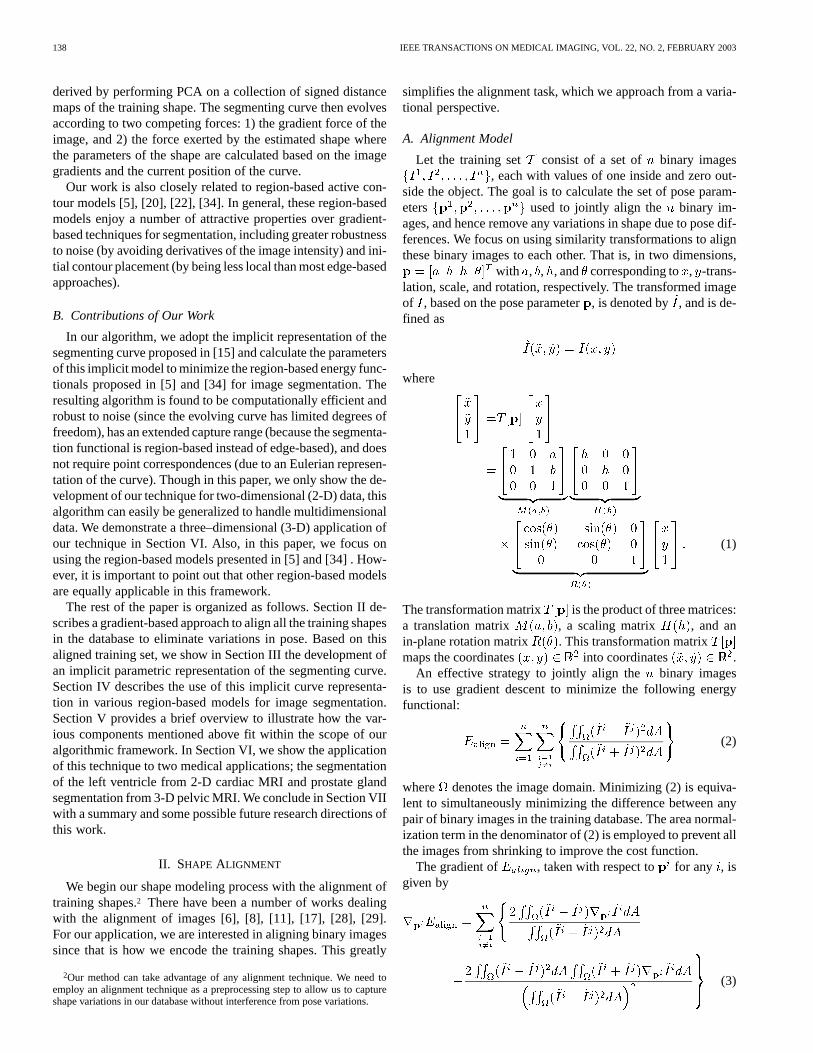
An effective strategy to jointly align the binary imagesis to use gradient descent to minimize the following energyfunctional:

(2)

where denotes the image domain. Minimizing (2) is equiva-lent to simultaneously minimizing the difference between anypair of binary images in the training database. The area normal-ization term in the denominator of (2) is employed to prevent allthe images from shrinking to improve the cost function.

The gradient of , taken with respect to for any , isgiven by

(3)

TSAI et al.: A SHAPE-BASED APPROACH TO THE SEGMENTATION OF MEDICAL IMAGERY USING LEVEL SETS 139

Fig. 1. Training data: 12 2-D binary shape models of the fighter jet.

Fig. 2. Alignment results of the above 12 2-D shape models of the fighter jet.

where is the gradient of the transformed imagetakenwith respect to the pose parameter. Using the chain rule, theth component of is given by

where

(4a)

(4b)

(4c)

(4d)

The matrix derivatives in (4) are taken componentwise. Sincethe solution of this alignment problem is under-determined, weregularize the problem by keeping the initial pose of one ofthe shapes fixed and calculating the pose parameters for the re-maining shapes using the above approach. The initial poses ofthe training shapes in are employed as the starting point forthe alignment process and gradient descent is performed untilconvergence.

To illustrate this alignment process, a training set, consistingof 12 binary representations of fighter jets, is shown in Fig. 1. Inthis example, the pose parameter of the fighter jet at the far leftside of the figure is chosen to be fixed, i.e., .The aligned version of this data set is shown in Fig. 2. Notethat all the aligned fighter jets share roughly the same center,are pointing in the same direction, and are approximately equalin size. One way to judge the effectiveness of this alignmentprocess is to assess the amount of overlap between the shapeswithin the database before and after the alignment process. Theprealignment overlap image, shown in Fig. 3(a), is generatedby stacking together all the binary fighter jets within the data-base prior to alignment (i.e., the fighter jets shown in Fig. 1),and adding them together in a pixelwise fashion. The postalign-ment overlap image, shown in Fig. 3(b), is generated in a sim-ilar fashion except that the binary fighter jets used to calculatethe overlap image have already been aligned. Specifically, thefighter jets used in this case are the ones shown in Fig. 2. Bycomparing the two overlap images, there is a dramatic increase

(a) (b)

Fig. 3. Comparison of the amount of shape overlap in the “fighter” database(a) before alignment and (b) after alignment.

in the amount of overlap between the shapes after the alignmentprocess suggesting that this method is an effective alignmenttechnique.

B. Multiresolution Alignment

The nature of the gradient descent approach we just describedallows for only infinitesimal updates of the pose parameters,thus giving rise to slow convergence properties and increasedsensitivity to local minima. These unattractive features are es-pecially evident when trying to align large and complicated ob-jects. One standard extension to enhance alignment algorithmsis to utilize a multiresolution approach. The basic idea behindthis approach is to employ a coarsened representation of thetraining set to obtain a good initial estimate of the pose param-eters. We then progressively refine these pose estimates as theresolution of the objects is increased.

Specifically, given a set of training objects, we repeatedlysubsample all the objects within the training set by a factor oftwo in each axis direction to obtain a collection of training setswith varying resolutions. Initial alignment is performed on thecoarsest resolution set of objects to obtain a good initial esti-mate of the pose parameters. Operating at such a coarse scale,we reduce the number of updates required for alignment (sincethe domain of the image is reduced) and the sensitivity of thealgorithm to local minima (by allowing the parameter searchto be less local). More importantly though, the computationalburden of alignment at each gradient step is substantially re-duced, mostly due to the decreased computational cost associ-ated with calculating (3) on a coarser grid. The pose parametersestimated on this coarsened set of training objects are appropri-ately scaled to serve as the starting pose estimates for the next


Fig. 4. Training data: 12 2-D binary shape models of the number four with size of 200� 200 pixels.

Fig. 5. Lowest resolution representation of the above training data with size of 50� 50 pixels.

Fig. 6. Alignment results of the above 50� 50 shape models of the number four.

Fig. 7. Coarse-to-fine multiresolution refinement results of the 200� 200 shape models of the number four.

higher resolution set of objects.3 By providing a good startingestimate of the pose parameters at this new scale, only a smallnumber of updates are required for convergence. This processof using the pose estimate at one resolution as the starting posefor the next finer resolution is repeated until the finest resolu-tion set of objects is reached. To illustrate this multiresolutionapproach, we show in Fig. 4 a set of 12 binary representationsof the number four. The fours are difficult objects to align dueto the complicated structure of these objects. Fig. 5 shows thissame data set with each shape down sampled by a factor of fourin each direction. Initially, we align the fours in this reducedimage domain. The results of this alignment are shown in Fig. 6.Next, we appropriately scale the pose parameters to serve as thestarting pose for the next higher resolution. We continue thisprocess until the finest resolution training set is reached. Thefinal alignment results are shown in Fig. 7. Fig. 8 shows theprealignment and postalignment overlap images of the numberfour to visually demonstrate the effectiveness of this alignmentprocess.

III. I MPLICIT PARAMETRIC SHAPE MODEL

As mentioned earlier, a popular and natural approach to rep-resent shapes is via point models where a set of marker points isused to describe the boundaries of the shape. This approach suf-fers from problems such as numerical instability, inability to ac-curately capture high curvature locations, difficulty in handlingtopological changes, and the need for point correspondences.To overcome these problem, we utilize an Eulerian approach toshape representation based on the level set methods of Osherand Sethian [19].

3Only the translational components of the pose are scaled up. The scaling androtational components of the pose remain fixed.

(a) (b)

Fig. 8. Comparison of the amount of shape overlap in the “four” database(a) before alignment and (b) after alignment.

A. Shape Parameters

Following the lead of [15] and [19], we choose the signeddistance function4 as our representation for shape. In particular,the boundaries of each of thealigned shapes in the database5

are embedded as the zero level set ofseparate signed distancefunctions with negative distances assignedto the inside and positive distances assigned to the outside ofthe object. Using the technique developed in [15], we compute

, the mean level set function of the shape database, as the av-erage of these signed distance functions, . Toextract the shape variabilities, is subtracted from each of the

signed distance functions to createmean-offset functions. These mean-offset functions are then used

to capture the variabilities of the training shapes.

4The signed distance(p) from an arbitrary pointp to a known surfaceZis the distance betweenp and the closest pointz in Z , multiplied by 1 or�1,depending on which side of the surfacep lies in [1].

5The shapes in the database are aligned by employing the method presentedin Section II.


Fig. 9. Three-dimensional visualization of the fighter jet shape variability. (a) The mean level set function��. (b) Three-dimensional illustration of+1� � .(c) Level set of+1� variation of the first principal mode. (d) Three-dimensional illustration of�1� � . (e) Level set of�1� variation of the first principal mode.

Specifically, we form column vectors, , consisting ofsamples of each (using identical sample locations for eachfunction). The most natural sampling strategy is to utilize the

rectangular grid of the training images to generatelexicographically ordered samples (where the

columns of the image grid are sequentially stacked on top of oneother to form one large column). Next, define the shape-vari-ability matrix as

An eigenvalue decomposition is employed to factoras

(5)

where is an matrix whose columns represent theorthogonal modes of variation in the shape andis an

diagonal matrix whose diagonal elements representthe corresponding nonzero eigenvalues. Theelements ofthe th column of , denoted by , are arranged back intothe structure of the rectangular image grid (byundoing the earlier lexicographical concatenation of the gridcolumns) to yield , the th principal mode or eigenshape.Based on this approach, a maximum ofdifferent eigenshapes

are generated.Note that in most cases, the dimension of the matrix

is large so the calculation of the eigen-

vectors and eigenvalues of this matrix is computationallyexpensive. In practice, the eigenvectors and eigenvalues of

can be efficiently computed from a much smallermatrix given by

It is straightforward to show that if is an eigenvector ofwith corresponding eigenvalue, then is an eigenvector of

with eigenvalue (see [14] for a proof).Let , which is selected prior to segmentation, be the

number of modes to consider. Choosing the appropriatein ourmodel is difficult and beyond the scope of this paper. Suffice it tosay that should be chosen large enough to be able to capturethe prominent shape variations present in the training set, butnot too large that the model begins to capture intricate detailsparticular to a certain training shape.6 In all of our examples, wechose empirically. We now introduce a new level set function

(6)

6One way to choose the value ofk is by examining the eigenvalues of the cor-responding eigenvectors. In some sense, the size of each eigenvalue indicates theamount of influence or importance its corresponding eigenvector has in deter-mining the shape. Perhapes by looking at a historgram of the eigenvalues, onecan determine the threshold for determining the value ofk. However, this ap-proach would be difficult to implement as the threshold value fork varies foreach application. In any case, there is no universalk that can be set.


where are the weights for the eigen-shapes with the variances of these weightsgiven by the eigenvalues calculated earlier. We propose to usethis newly constructed level set functionas our implicit rep-resentation of shape. Specifically, the zero level set ofde-scribes the shape with the shape’s variability directly linked tothe variability of the level set function. Therefore, by varying

, we vary which indirectly varies the shape. Note that theshape variability we allow in this representation is restricted tothe variability given by the eigenshapes.

Fig. 9 provides some intuition as to how the level set repre-sentation of (6) captures shape variability. The set of 12 fighterjets shown in Fig. 2 is used as the shape training set to obtain

and . Fig. 9(a) showsthe mean level set function with the red curve outlining thezero level set of . Fig. 9(b) shows the function withthe magenta curve outlining the zero crossings of this function.Notice that most of the spatial variations associated with thisfunction lie in the area corresponding to the wings of the fighterjet. Specifically, a large rising “hump” can be seen in those areas.When this function is added to, a new level set representa-tion of the fighter jet is obtained. This new level set function isshown in Fig. 9(c) with the blue curve outlining the zero levelset. As expected, adding to causes the wing size toshrink, thus yielding a new fighter jet with a much smaller wingspan. In Fig. 9(d), we show the function with the ma-genta curve outlining the zero crossings of this function. This issimply the negative of Fig. 9(b) and hence adding this functionto causes the wing span of the fighter jet to increase. Thisresulting level set function is illustrated in Fig. 9(e) with theblue curve outlining the zero level set. To further illustrate theparametric shape encoding scheme of (6), we show in Fig. 10the mean shape of the fighter jet as well as its shape varia-tions based on varying its first three principal modes by .As another demonstration, we employ the set of training shapesshown in Fig. 7 to obtain an implicit parametric representationof the number four. Fig. 11 shows the mean shape of the numberfour as well as its shape variations based on varying its first threeprincipal modes by . Notice that by varying the first twoprincipal modes, the shape of the number four changes topologygoing from two curves to one curve. This is an additional advan-tage of using the Eulerian framework for shape representationas it can handle topological changes in a seamless fashion. Thisability is of value for biomedical applications. One such applica-tion is the tracking of changes in multiple sclerosis lesions overtime (as they shrink, migrate, split, disappear, etc.). Another isin the segmentation of the pancreas which often presents as onesolid organ. But at times, the pancreas does not fuse in uteroand hence presents as two separate lobes which may requiresegmentation algorithms that can deal with topology changes.Another application might be in segmenting skin lesions. Someskin pathologies can present both as one confluent lesion or asan island of lesions.

B. Pose Parameters

At this point, our implicit representation of shape cannot ac-commodate shape variabilities due to differences in pose. Tohave the flexibility of handling pose variations,is added asanother parameter to the level set function of (6). With this new

addition, the implicit description of shape is given by the zerolevel set of the following function:

(7)

where

with defined earlier in (1). The addition of to our para-metric shape model enables us to accomodate a larger class ofobjects. In particular, the model can now handle object shapesthat may differ from each other in terms of scale, orientation,or center location. In Section IV, we describe howand areoptimized, via coordinate descent, for image segmentation.

IV. REGION-BASED MODELS FORSEGMENTATION

In region-based segmentation models [5], [20], [22], [34],the evolution of the segmenting curve depends upon the pixelintensities within entire regions. That is, region-based modelsregard an image as the composition of a finite number of re-gions and rely on regional statistics for segmentation. The sta-tistics of entire regions (such as sample mean and variance) areused to direct the movement of the curve toward the bound-aries of the image. This is in sharp contrast to edge-based seg-mentation models [2], [3], [9], [12], [13], [16], [24], [25], [32]where the evolution of the curve depends strictly on nearbypixel intensities (i.e., gradient information). As a result, region-based models are more global than edge-based models. Fur-thermore, because of the global nature of region-based models,these models do not require the use of inflationary terms com-monly employed by edge-based techniques to drive the curve to-ward image boundaries. Region-based models are also more ro-bust to noise since they do not employ gradient operators, whichare inherently sensitive to noise, to explicitly detect the loca-tion of edges. In this section, we present three recently devel-oped region-based models for segmentation and describe howthese models fit within the scope of our shape-based curve evo-lution framework. Specifically, in this section, we present theChan-Vese model, the binary mean model, and the binary vari-ance model for image segmentation. However, instead of de-riving the evolution equation for the curves used to segment theimage (which is the original design of these models), we derivegradient descent equations used to optimize the shape and poseparameters that indirectly describe the segmenting curve.

A. Description of the Models

We begin with a simple synthetic example to present howregion-based segmentation models are incorporated intoour model-based algorithm. Assume that the domain of theobserved image is formed by two regions distinguishableby some region statistic (e.g., sample mean or variance). Wewould like to segment this image via the curve, which in ourframework, is represented by the zero level set of, i.e.,


Moreover, as a result of this implicit parametric representationof , the regions inside and outside the curve, denoted, respec-tively, by and , are given by

In our algorithmic framework, we calculate the parameters ofto vary and hence segment the image. These param-

eters, and , are obtained by minimizing region-based energyfunctionals that are constructed using various image statistics.Some useful image statistics, written in terms of , are

area in

area in

sum intensity in

sum intensity in

sum of squared intensity in

sum of squared intensity in

average intensity in

average intensity in

sample variance in

sample variance in

where the Heaviside function is given by

ifif .

Chan and Vese in [5], and Yezziet al. in [34] proposed pure re-gion-based models to segmentusing these region statistics.Below, we provide descriptions of their models, describe therole of and in these models, and detail the optimization ofthese models with respect to and (instead of ) for imagesegmentation. As detailed in Section III, by calculating the pa-rameters and that optimize the segmentation energy func-tionals, we have implicitly determined the segmenting curve.Thus, our segmentation approach can be considered as a param-eter optimization technique.

1) The Chan-Vese Model:Chan and Vese in [5] proposedthe following energy functional for segmenting:

which is equivalent, (up to a term which does not depend uponthe evolving curve), to the energy functional below

(8)

The Chan-Vese energy functional can be viewed as a piece-wise constant generalization of the Mumford-Shah functional[18]. Gradient descent is employed to search for the parame-ters and that minimize to implicitly determine the seg-

menting curve. The gradients of , taken with respect toand , are given by

(9a)

(9b)

2) The Binary Mean Model:A different strategy was pro-posed by Yezziet al. in [34] to segment . They propose toevolve so as to maximize the distance betweenand . Anatural cost functional they employed is to minimize the fol-lowing:

(10)

The authors in [34] called this thebinary model(since it isinitially designed to segment images consisting of two distinctbut constant intensity regions). Once again, gradient descent isemployed to calculate the parametersand that minimize

to implicitly determine the segmenting curve. The gra-dients of , taken with respect to and , are given by

(11a)

(11b)

3) The Binary Variance Model:So far, we have focused onusing the mean as the image statistic in differentiating the tworegions in . Other image statistics can also be used in a re-gion-based segmentation model. For example, Yezziet al. in[34] proposed a segmentation model based on image variances.Consider the following energy functional for segmentation:

(12)

The design of this model is to partition an image into two re-gions, one of low variance and one of high variance, by max-imally separating the sample variances inside and outside thecurve. The gradients of , taken with respect to and

, are given by

(13a)

(13b)

where


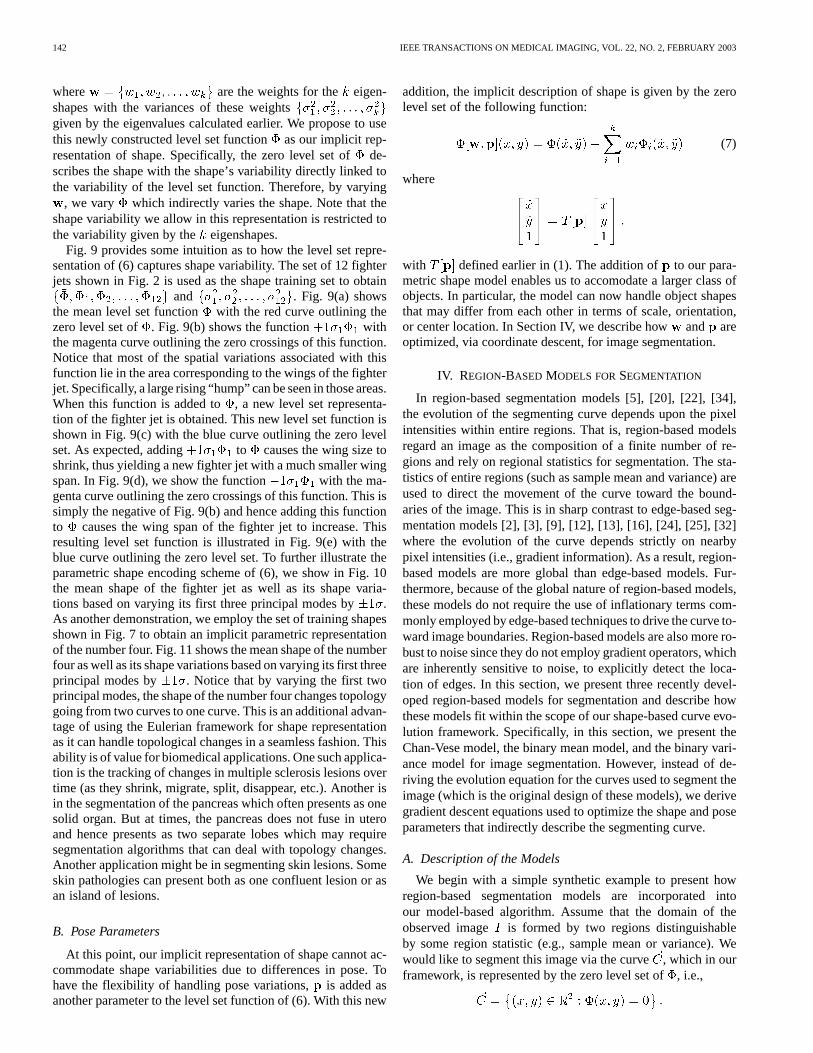
B. Gradients of Region Statistics

As shown in (9), (11), and (13), to update the shape and poseparameters via gradient descent, the gradients of region statis-tics , , , , , and , taken with respect to and

, are required. Defining the one-dimensional Dirac measureconcentrated at zero by

we can now express theth component of each of the gradientterms in (9), (11), and (13) as line integrals along

where

with previously defined in (4).

C. Parameter Optimization Via Gradient Descent

The gradients of the various energy functionals taken withrespect to and are given by (9), (11), and (13). For concise-ness of notation, denote and as the gradients of anyof the above energy functionals taken with respect toand ,respectively. With this introduction, the update equations for theshape and pose parameters in our gradient descent approach aregiven by

where and are positive step-size paramters, and anddenote the values of and at the th iteration, respec-

tively. The updated shape and pose parameters are then usedto implicitly determine the updated location of the segmentingcurve.

It is important to note that no special numerics were requiredin our proposed technique as it does not involve any partial dif-ferential equations. This results in fast and simple implementa-tion of our methodology. In fact, this is one of the main departurebetween our model and the earlier one put forth by Leventonet al. [15]

D. Extension to Three Dimensions

The generalization of this algorithm to three dimensions isstraightforward. The pose parameter is expanded to consist of

seven terms: , , and translation; pitch; yaw; roll; and mag-nification. The shape alignment strategy is to jointly align the

binary volumetric data via gradient descent. Signed distancefunction is similarily employed to represent the 3-D shapes. Inparticular, the bounding surfaces of each shape is embedded asthe zero level set of a signed distance function with negativedistances assigned to the inside and positive distances assignedto the outside of the 3-D object. The 3-D shape parameters arederived in a similar fashion as the 2-D shape parameters. How-ever, these 3-D shape parameters implicitly describe a 3-D seg-menting surface rather than a 2-D segmenting curve. The regionstatistics used in the region-based models for segmentation arenow calculated over an entire volume rather than over an entireregion.

E. Illustration of the Models Using Synthetic Data

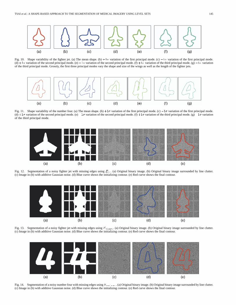
Figs. 12–14 show the use of , , and forsegmentation. We show in Fig. 12(a) a fighter jet (that is not partof the fighter jet database of Fig. 1). Fig. 12(b) shows the samefighter jet surrounded by horizontal and vertical line clutter. Thepresence of these lines creates missing edges in the fighter jetwhich can cause problems in conventional segmentation algo-rithms that do not rely on prior shape information. Fig. 12(c)shows this line-cluttered fighter jet image contaminated by ad-ditive Gaussian noise. The goal is to segment the fighter jet fromthis noisy test image. Knowinga priori that the object in theimage is a fighter jet, we employ the database shown in Fig. 2 toderive an implicit parametric curve model for the fighter jet [inthe form of (7)]. In this example, we use . The zero levelset of is employed as the starting curve which is illustrated inFig. 12(d). The parameters of the segmenting curve,and ,are calculated to minimize . Fig. 12(e) shows the final shapeand position of the segmenting curve. Notice that we are able tosuccessfully find the boundaries of the fighter jet without beingdistracted by the line clutter. In Fig. 13, we show a slight variantof the experiment just described. Specifically, a new fighter jet(which is also not part of the database of Fig. 1) is employedas the object in the test image, and is employed as thesegmentation functional. Using the sameas before, we are able to successfully segment this new object.

Fig. 14 shows a different experiment. The object in this ex-periment is the number four which is shown in Fig. 14(a). Ver-tical and horizontal lines are again added to this image to createmissing edges in the object. The resulting line-cluttered image isshown in Fig. 14(b). This binary mask is used to create the vari-ance image shown in Fig. 14(c) which consists of two regions,each of identical means but of different variances. The goal is tosegment the object from this noisy test image. Knowinga priorithat the object in the image is a handwritten four, we employ thedatabase of fours, shown in Fig. 7, to obtain the mean shape andthe eigenshapes for our implicit representation of the object. Asbefore, we use . The zero level set of is employed as thestarting curves as illustrated in Fig. 14(d). Notice in this figurethat two curves are used to describe the starting shape. Becausethe image statistic that characterizes the two regions in this testimage is variance, the parameters of the segmenting curve,and , are calculated to minimize . Fig. 14(e) shows thesuccessful segmentation of the number four image. Notice thatwithout any additional effort, the two starting curves merged toform one single segmenting curve at the end.


Fig. 10. Shape variability of the fighter jet. (a) The mean shape. (b)+1� variation of the first principal mode. (c)�1� variation of the first principal mode.(d)+1� variation of the second principal mode. (e)�1� variation of the second principal mode. (f)+1� variation of the third principal mode. (g)�1� variationof the third principal mode. Grossly, the first three principal modes vary the shape and size of the wings as well as the length of the fighter jets.

Fig. 11. Shape variability of the number four. (a) The mean shape. (b)+1� variation of the first principal mode. (c)�1� variation of the first principal mode.(d)+1� variation of the second principal mode. (e)�1� variation of the second principal mode. (f)+1� variation of the third principal mode. (g)�1� variationof the third principal mode.

Fig. 12. Segmentation of a noisy fighter jet with missing edges usingE . (a) Original binary image. (b) Original binary image surrounded by line clutter.(c) Image in (b) with additive Gaussian noise. (d) Blue curve shows the initializing contour. (e) Red curve shows the final contour.

Fig. 13. Segmentation of a noisy fighter jet with missing edges usingE . (a) Original binary image. (b) Original binary image surrounded by line clutter.(c) Image in (b) with additive Gaussian noise. (d) Blue curve shows the initializing contour. (e) Red curve shows the final contour.

Fig. 14. Segmentation of a noisy number four with missing edges usingE . (a) Original binary image. (b) Original binary image surrounded by line clutter.(c) Image in (b) with additive Gaussian noise. (d) Blue curve shows the initializing contour. (e) Red curve shows the final contour.


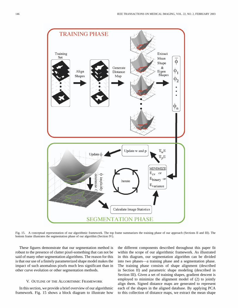
Fig. 15. A conceptual representation of our algorithmic framework. The top frame summarizes the training phase of our approach (Sections II and III).Thebottom frame illustrates the segmentation phase of our algorithm (Section IV).

These figures demonstrate that our segmentation method isrobust to the presence of clutter pixel-something that can not besaid of many other segmentation algorithms. The reason for thisis that our use of a finitely parameterized shape model makes theimpact of such anomalous pixels much less significant than inother curve evolution or other segmentation methods.

V. OUTLINE OF THE ALGORITHMIC FRAMEWORK

In this section, we provide a brief overview of our algorithmicframework. Fig. 15 shows a block diagram to illustrate how

the different components described throughout this paper fitwithin the scope of our algorithmic framework. As illustratedin this diagram, our segmentation algorithm can be dividedinto two phases—a training phase and a segmentation phase.The training phase consists of shape alignment (describedin Section II) and parametric shape modeling (described inSection III). Given a set of training shapes, gradient descent isemployed to minimize the alignment model of (2) to jointlyalign them. Signed distance maps are generated to representeach of the shapes in the aligned database. By applying PCAto this collection of distance maps, we extract the mean shape


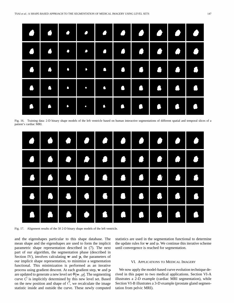
Fig. 16. Training data: 2-D binary shape models of the left ventricle based on human interactive segmentations of different spatial and temporal slices of apatient’s cardiac MRI.

Fig. 17. Alignment results of the 50 2-D binary shape models of the left ventricle.

and the eigenshapes particular to this shape database. Themean shape and the eigenshapes are used to form the implicitparametric shape representation described in (7). The nextpart of our algorithm, the segmentation phase (described inSection IV), involves calculating and , the parameters ofour implicit shape representation, to minimize a segmentationfunctional. This minimization is performed as an iterativeprocess using gradient descent. At each gradient step,andare updated to generate a new level set . The segmentingcurve is implicitly determined by this new level set. Basedon the new position and shape of, we recalculate the imagestatistic inside and outside the curve. These newly computed

statistics are used in the segmentation functional to determinethe update rules for and . We continue this iterative schemeuntil convergence is reached for segmentation.

VI. A PPLICATIONS TOMEDICAL IMAGERY

We now apply the model-based curve evolution technique de-rived in this paper to two medical applications. Section VI-Aillustrates a 2-D example (cardiac MRI segmentation), whileSection VI-B illustrates a 3-D example (prostate gland segmen-tation from pelvic MRI).


(a) (b)

Fig. 18. Comparison of the amount of shape overlap in the cardiac database(a) before alignment and (b) after alignment.

A. A 2-D Example: Left Ventricle Segmentation of CardiacMRI

Cardiac MRI is an important clinical tool used to providefour–dimensional (4-D) (temporal as well as spatial) informa-tion about the heart. Typically, one study generates 80–120 2-Dimages of a patient’s heart. In a variety of clinical scenarios(such as assessing cardiac function and diagnosing cardiac dis-eases), it is important to extract the boundaries of the left ven-tricle from this data set. For example, the segmentation of theleft ventricle is a prerequisite in calculating important physio-logical parameters such as ejection fraction and stroke volume.Manual tracing of the left ventricle from such a large data set isboth tedious and time-consuming. A robust automated segmen-tation algorithm of the left ventricle would be preferred.

Conventional automated segmentation techniques usuallyencounter difficulties in segmenting the left ventricle because1) the intensity contrast between the ventricle and the myo-cardium is low (due to the smearing of the blood pool in theventricle into the myocardium), and 2) the boundaries of theleft ventricle are missing at certain locations due to the presenceof protruding papillary muscles which have the same intensityprofile as the myocardium.

In the experiment to illustrate our technique, we equally di-vided the 100 2-D images from a single patient’s cardiac MRIinto two sets: a training set and a test set. Fifty 4-D interactivesegmentations of the left ventricle from the training set form the2-D shape database shown in Fig. 16. This particular databaseis employed to allow our model to capture both the spatial andthe temporal variations of the left ventricle. Fig. 17 shows thealigned version of this database. Fig. 18 compares the overlapimages of the left ventricle database before and after alignment.Using the aligned database, we derived the mean level set andthe eigenshapes to form the implicit shape model of the left ven-tricle using . Fig. 19 shows the mean shape of the leftventricle as well as its shape variations by varying the first threeeigenshapes by . The parameters of this implicit parametricrepresentation are calculated to minimize using statisticscalculated in the entire region both inside and outside the curve.Fig. 20 shows the segmentation result of the testing set by our al-gorithm (red curves). These results are comparable with the onesgiven by a 4-D interactive cardiac MRI segmenter [33] (greencurves) which utilizes a 4-D conformal surface shrinking tech-nqiue based upon the models outlined in [32].

B. A 3-D Example: Prostate Segmentation of Pelvic MRITaken With Endorectal Coil

Pelvic MRI, when taken in conjunction with an endorectalcoil (ERC) (a receive-only surface coil placed within therectum) using T1 and T2 weighting, provides high-resolutionimages of the prostate with smaller field of view and thinnerslice thickness than previously attainable. Because of thehigh-quality anatomical images obtainable by this technique,it may become the imaging modality of choice in the futurefor detection and staging of prostate cancer [7], [31]. Forassignment of appropriate radiation therapy after cancerdetection, the segmentation of the prostate gland from thesepelvic MRI images is required. Manual outlining of sequentialcross-sectional slices of the prostate images is currently used toidentify the prostate gland and its substructures, but this processis difficult, time-consuming, and tedious. The idea of beingable to automatically segment the prostate is very attractive.

Automatic segmentation of the prostate is difficult becausethe prostate is a small glandular structure buried deep withinthe pelvic region and surrounded by a variety of different tis-sues which show up as varying intensity levels on the MRI.This segmentation problem is further complicated by an arti-fact called the near-field effect which is caused by the use ofthe ERC. The near-field effect causes an intensity artifact to ap-pear in the tissues surrounding the ERC. This can be seen as awhite circular halo surrounding the rectum in each image sliceof Figs. 27 and 30. The intensity artifact can bleach out the bor-ders of the prostate near the rectum, making the prostate seg-mentation problem even more difficult.

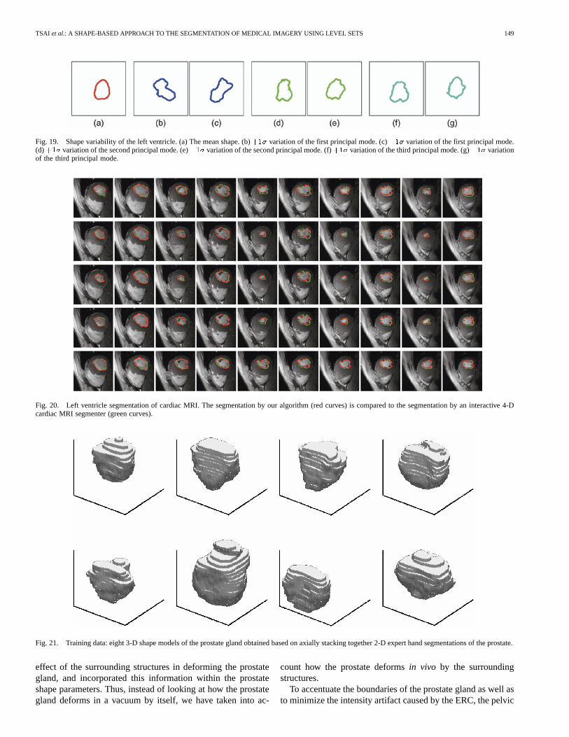
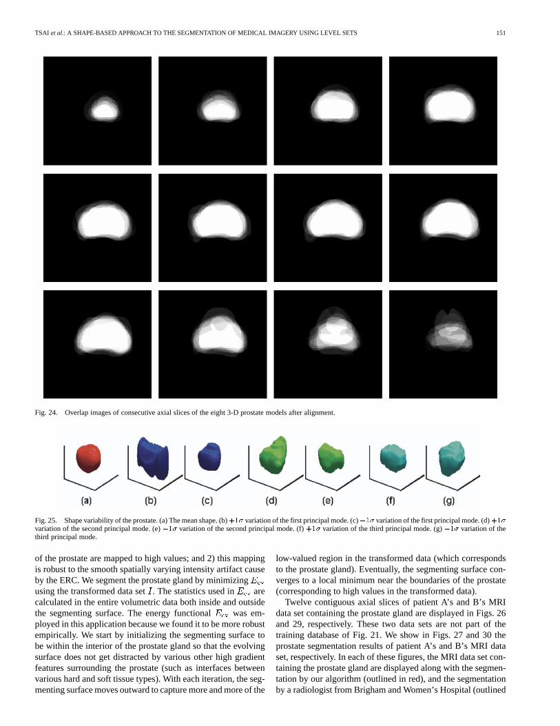
We employ a 3-D version of our shape-based curve evolutiontechnique to segment the prostate gland. By utilizing a surface(instead of a curve), the segmentation algorithm is able to utilizethe full 3-D spatial information to extract the boundaries of theprostate gland. Fig. 21 shows the prostate training data we usewhich consists of eight 3-D binary shape models of the prostategland-obtained by stacking together 2-D expert hand segmen-tations of eight patients’ pelvic MRIs taken with an ERC. Thealignment results of these 3-D models are shown in Fig. 21. Toevaluate the alignment process, Fig. 23 shows 12 consecutiveaxial slice overlap images of the eight 3-D prostate gland modelsprior to alignment. And Fig. 24 shows the same 12 overlap im-ages after alignment for comparison. Prior to shape training,these 3-D shape models are smoothed to remove the “step-like”artifact along the axial direction of the prostate. Based on these3-D models, we derived the mean level set and the eigenshapesto form the implicit shape model of the prostate gland using

. Fig. 25 shows the mean shape of the prostate gland aswell as its shape variations based on varying the first three eigen-shapes by .

In this particular application, it is important to realize thatdespite the fact that the prostate gland is mostly deformed byits neighboring structures, the prostate shape parameters arestill very important in describing its shape. In our method, bycapturing how its surrounding structures deform the prostategland, we obtain shape parameters that can effectively describethe deformations of the prostate gland. Specifically, we lookedat a population of patients and learned the total net resultant


Fig. 19. Shape variability of the left ventricle. (a) The mean shape. (b)+1� variation of the first principal mode. (c)�1� variation of the first principal mode.(d)+1� variation of the second principal mode. (e)�1� variation of the second principal mode. (f)+1� variation of the third principal mode. (g)�1� variationof the third principal mode.

Fig. 20. Left ventricle segmentation of cardiac MRI. The segmentation by our algorithm (red curves) is compared to the segmentation by an interactive4-Dcardiac MRI segmenter (green curves).

Fig. 21. Training data: eight 3-D shape models of the prostate gland obtained based on axially stacking together 2-D expert hand segmentations of the prostate.

effect of the surrounding structures in deforming the prostategland, and incorporated this information within the prostateshape parameters. Thus, instead of looking at how the prostategland deforms in a vacuum by itself, we have taken into ac-

count how the prostate deformsin vivo by the surroundingstructures.

To accentuate the boundaries of the prostate gland as well asto minimize the intensity artifact caused by the ERC, the pelvic


Fig. 22. Alignment results of the eight 3-D shape models of the prostate gland.

Fig. 23. Overlap images of consecutive axial slices of the eight 3-D prostate models prior to alignment.

MRI data set is transformed to a bimodal data setbyapplying the following map:

where here denotes a 3-D gradient operator. This mappingwas employed because: 1) the interior of the prostate is homo-geneous in intensity, so with this mapping, the interior regionsof the prostate are mapped to low values while the boundaries


Fig. 24. Overlap images of consecutive axial slices of the eight 3-D prostate models after alignment.

Fig. 25. Shape variability of the prostate. (a) The mean shape. (b)+1� variation of the first principal mode. (c)�1� variation of the first principal mode. (d)+1�variation of the second principal mode. (e)�1� variation of the second principal mode. (f)+1� variation of the third principal mode. (g)�1� variation of thethird principal mode.

of the prostate are mapped to high values; and 2) this mappingis robust to the smooth spatially varying intensity artifact causeby the ERC. We segment the prostate gland by minimizingusing the transformed data set. The statistics used in arecalculated in the entire volumetric data both inside and outsidethe segmenting surface. The energy functional was em-ployed in this application because we found it to be more robustempirically. We start by initializing the segmenting surface tobe within the interior of the prostate gland so that the evolvingsurface does not get distracted by various other high gradientfeatures surrounding the prostate (such as interfaces betweenvarious hard and soft tissue types). With each iteration, the seg-menting surface moves outward to capture more and more of the

low-valued region in the transformed data (which correspondsto the prostate gland). Eventually, the segmenting surface con-verges to a local minimum near the boundaries of the prostate(corresponding to high values in the transformed data).

Twelve contiguous axial slices of patient A’s and B’s MRIdata set containing the prostate gland are displayed in Figs. 26and 29, respectively. These two data sets are not part of thetraining database of Fig. 21. We show in Figs. 27 and 30 theprostate segmentation results of patient A’s and B’s MRI dataset, respectively. In each of these figures, the MRI data set con-taining the prostate gland are displayed along with the segmen-tation by our algorithm (outlined in red), and the segmentationby a radiologist from Brigham and Women’s Hospital (outlined


Fig. 26. Prostate images of patient A. These images represent consecutive axial slices of the prostate. Segmenting curves were not superimposed on the imagesfor better visualization of the prostate organ.

Fig. 27. Prostate segmentation of patient A. The segmentation by the radiologist (green curves) is compared to the segmentation by our algorithm (redcurves).

in green). Another radiologist, also from Brigham and Women’sHospital, rated the first radiologist’s segmentation of data set Ato be slightly better than our algorithm’s, and rated our algo-rithm’s segmentation of data set B to be slightly better than theradiologist’s. For visual comparison, Figs. 28 and 31 show the3-D models of the prostate gland generated by our algorithmand by stacking together 2-D expert hand segmentations. No-tice that by employing a surface to capture the prostate gland,our 3-D model does not display any of the “step-like” artifactsthat mar the radiologist’s 3-D rendition of the prostate gland. Inaddition, working in 3-D space allows our algorithm to utilizethe full 3-D structural information of the prostate for segmen-tation (instead of just the information from neighboring sliceswhich are typically used by the radiologists).

VII. CONCLUSION AND FUTURE RESEARCHDIRECTIONS

We have outlined a statistically robust and computationallyefficient model-based segmentation algorithm using an implicitrepresentation of the segmenting curve. Because this implicitrepresentation is set in an Eulerian framework, it does not re-quire point correspondences during the training phase of the al-gorithm and can be used to handle topological changes of the

(a) (b)

Fig. 28. Three-dimensional models of patient A’s prostate gland. (a) Based onour segmentation algorithm. (b) Based on the radiologist’s segmentation.

segmenting curve in a seamless fashion. This algorithmic frame-work is capable of segmenting images contaminated by heavynoise and delineate structures complicated by missing or diffuseedges. In addition, this framework is flexible, both in terms ofits ability to model and segment complicated shapes (as longas the shape variations are consistent with the training data), aswell as its ability to accommodate the segmentation of multidi-mensional data sets. Furthermore, by employing a region-basedsegmentation functional, our algorithm is more global, exhibits


Fig. 29. Prostate images of patient B. These images represent consecutive axial slices of the prostate. Segmenting curves were not superimposed on the imagesfor better visualization of the prostate organ.

Fig. 30. Prostate segmentation of patient B. The segmentation by the radiologist (green curves) is compared to the segmentation by our algorithm (redcurves).

(a) (b)

Fig. 31. Three–dimensional models of patient B’s prostate gland. (a) Basedon our segmentation algorithm. (b) Based on the radiologist’s segmentation.

increased robustness to noise, displays extensive capture range,and is less sensitive to initial contour placements compared withother model-based segmentation algorithms.

The performance of our model-based curve evolution tech-nique depends largely upon how well the chosen set of statisticsis able to distinguish the various regions within a given image.In this paper, we detailed the use of means and variances asthe discriminating statistics. However, this approach may be ap-plied to any computed statistics. We are interested in extending

our method by constructing different segmentation functionalsbased on first (and maybe higher) order statistics such as skew-ness, kurtosis, and entropy.

In this paper, we discussed the use of signed distance func-tions as a way to represent shapes. However, because distancefunctions are not closed under linear operations, the level setrepresentation of our segmenting curve, based on the PCA ap-proach described in Section III, is not a distance function. Thisgives rise to an inconsistent framework for shape modeling. Thisintellectual issue remains an important and challenging problem(indeed one on which we are now working ourselves), but themethod developed in this paper stands on its performance inpractice.

ACKNOWLEDGMENT

The authors would like to thank the anonymous reviewers fortheir valuable comments and thoughtful suggestions.

REFERENCES

[1] G. Borgefors, “Distance transformations in digital images,”CVGIP:Image Understanding, vol. 34, pp. 344–371, 1986.

[2] V. Caselles, F. Catte, T. Coll, and F. Dibos, “A geometric model foractive contours in image processing,”Numerische Mathematik, vol. 66,pp. 1–31, 1993.


[3] V. Caselles, R. Kimmel, and G. Sapiro, “Geodesic snakes,”Int. J.Comput. Vis., 1998.

[4] A. Chakraborty, L. Staib, and J. Duncan, “An integrated approach toboundary finding in medical images,” inProc. IEEE Workshop Biomed-ical Image Analysis, 1994, pp. 13–22.

[5] T. Chan and L. Vese, “Active contours without edges,”IEEE Trans.Image Processing, vol. 10, pp. 266–277, Feb. 2001.

[6] Y. Chen, S. Thiruenkadam, H. Tagare, F. Huang, D. Wilson, and E.Geiser, “On the incorporation of shape priors into geometric active con-tours,” in Proc. IEEE Workshop Variational and Level Set Methods,2001, pp. 145–152.

[7] D. Cheng and C. Tempany, “MR imaging of the prostate and bladder,”Seminars Ultrasound, CT, MRI, vol. 19, no. 1, pp. 67–89, 1998.

[8] G. Christensenet al., “Consistent linear-elastic transformation for imagematching,” inLecture Notes in Computer Science, A. Kubaet al., Eds.,1999, vol. 1613, Information Processing in Medical Imaging (Proc. 16thInt. Conf.), pp. 224–237.

[9] L. Cohen, “On active contour models and ballooms,”CVGIP: ImageUnderstanding, vol. 53, pp. 211–218, 1991.

[10] T. Cootes, C. Taylor, D. Cooper, and J. Graham, “Active shape models-their training and application,”Comput. Vis. Image Understanding, vol.61, pp. 38–59, 1995.

[11] B. Frey and N. Jojic, “Estimating mixture models of images andinferring spatial transformations using the EM algorithm,” inProc.IEEE Conf. Computer Vision and Pattern Recognition, vol. 1, 1999, pp.416–422.

[12] M. Kass, A. Witkin, and D. Terzopoulos, “Snakes: Active contourmodels,”Int. J. Comput. Vis., vol. 1, pp. 321–331, 1987.

[13] S. Kichenassamy, A. Kumar, P. Olver, A. Tannenbaum, and A. Yezzi,“Conformal curvature flows: From phase transitions to active vision,”Arch. Rational Mech. Anal., vol. 134, pp. 275–301, 1996.

[14] M. Leveton, “Statistical models in medical image analysis,” Ph.D. dis-sertation, Massachusetts Inst. Technol, Dept. Elect. Eng., 2000.

[15] M. Leventon, E. Grimson, and O. Faugeras, “Statistical shape influencein geodesic active contours,” inProc. IEEE Conf. Computer Vision andPattern Recognition, vol. 1, 2000, pp. 316–323.

[16] R. Malladi, J. Sethian, and B. Vemuri, “Shape modeling with front prop-agation: A level set approach,”IEEE Trans. Pattern Anal. Machine In-tell., vol. 17, pp. 158–175, Feb. 1995.

[17] E. Miller, N. Matsakis, and P. Viola, “Learning from one examplethrough shared densities on transforms,” inProc. IEEE Conf. ComputerVision and Pattern Recognition, vol. 1, 2000, pp. 464–471.

[18] D. Mumford and J. Shah, “Optimal approximations by piecewisesmooth functions and associated variational problems,”Comm. PureAppl. Math., vol. 42, pp. 577–685, 1989.

[19] S. Osher and J. Sethian, “Fronts propagation with curvature dependentspeed: Algorithms based on Hamilton-Jacobi formulations,”J. Comput.Phys., vol. 79, pp. 12–49, 1988.

[20] N. Paragios and R. Deriche, “Geodesic Active Regions for Texture Seg-mentation,” INRIA, Sophia Antipolis, France, Res. Rep. 3440, 1998.

[21] A. Pentland and S. Sclaroff, “Closed-form solutions for physically basedshape modeling and recognition,”IEEE Trans. Pattern Anal. MachineIntell., vol. 13, pp. 715–729, July 1991.

[22] R. Ronfard, “Region-based strategies for active contour models,”Int. J.Comput. Vis., vol. 13, pp. 229–251, 1994.

[23] L. Staib and J. Duncan, “Boundary finding with parametrically de-formable contour models,”IEEE Trans. Pattern Anal. Machine Intell.,vol. 14, pp. 1061–1075, Nov. 1992.

[24] H. Tek and B. Kimia, “Image segmentation by reaction diffusion bub-bles,” inProc. Int. Conf. Computer Vision, 1995, pp. 156–162.

[25] D. Terzopoulos and A. Witkin, “Constraints on deformable models: Re-covering shape and nonrigid motion,”Artif. Intell., vol. 36, pp. 91–123,1988.

[26] A. Tsai, A. Yezzi, W. Wells, C. Tempany, D. Tucker, A. Fan, E. Grimson,and A. Willsky, “Model-based curve evolution technique for image seg-mentation,” inIEEE Conf. Computer Vision and Pattern Recognition,vol. 1, 2001, pp. 463–468.

[27] A. Tsai, A. Yezzi, and A. Willsky, “A curve evolution approach tosmoothing and segmentation using the mumford-shah functional,” inIEEE Conf. Computer Vision and Pattern Recognition, vol. 1, 2000, pp.1119–1124.

[28] T. Vetter, M. Jones, and T. Poggio, “A bootstrapping algorithm forlearning linear models of object classes,” inIEEE Conf. ComputerVision and Pattern Recognition, vol. 1, 1997, pp. 40–46.

[29] P. Viola and W. Wells, “Mutual information: An approach for the regis-tration of object models and images,”Int. J. Comput. Vis., 1997.

[30] Y. Wang and L. Staib, “Boundary finding with correspondence usingstatistical shape models,” inIEEE Conf. Computer Vision and PatternRecognition, 1998, pp. 338–345.

[31] T. Wong, G. Silverman, J. Fielding, C. Tempany, K. Hynynen, and F.Jolesz, “Open-configuration MR imaging, intervention, and surgery ofthe urinary tract,”Urologic Clin. No. Amer., vol. 25, pp. 113–122, 1998.

[32] A. Yezzi, S. Kichenassamy, A. Kumar, P. Olver, and A. Tannenbaum,“A geometric snake model for segmentation of medical imagery,”IEEETrans. Med. Imag., vol. 16, pp. 199–209, Apr. 1997.

[33] A. Yezzi and A. Tannenbaum, “4D active surfaces for cardiac seg-mentation,” Med. Image Computing Comput. Assist. Intervention, pp.667–673, 2002, submitted for publication.

[34] A. Yezzi, A. Tsai, and A. Willsky, “A statistical approach to snakes forbimodal and trimodal imagery,” inProc. Int. Conf. Computer Vision, vol.2, 1999, pp. 898–903.

Documents

A shape-based approach to the segmentation of medical ...ssg.mit.edu/group/alumni/atsai/Papers/TMI03.pdf · A Shape-Based Approach to the Segmentation of Medical Imagery Using