A short introduction to light and electron microscopy · 2. Light microscopy As mentioned above, light microscopes use light to illuminate an object and to generate an image of it

Microscopy Toolbox 2017

Center for Microscopy and Image Analysis

A short introduction to

light and electron microscopy


2 Center for Microscopy and Image Analysis

1. General Introduction

Microscopy enables a “direct” imaging of organisms, tissues, cells, organelles, molecular assemblies and even individual proteins. Analytical techniques as used in molecular biology provide a data set which represents cellu-lar processes in an abstract way. Therefore, microscopy was and still is an important, complementary technique to visualize the macro and/or microscopic structure and to assign structure to function and vice versa.

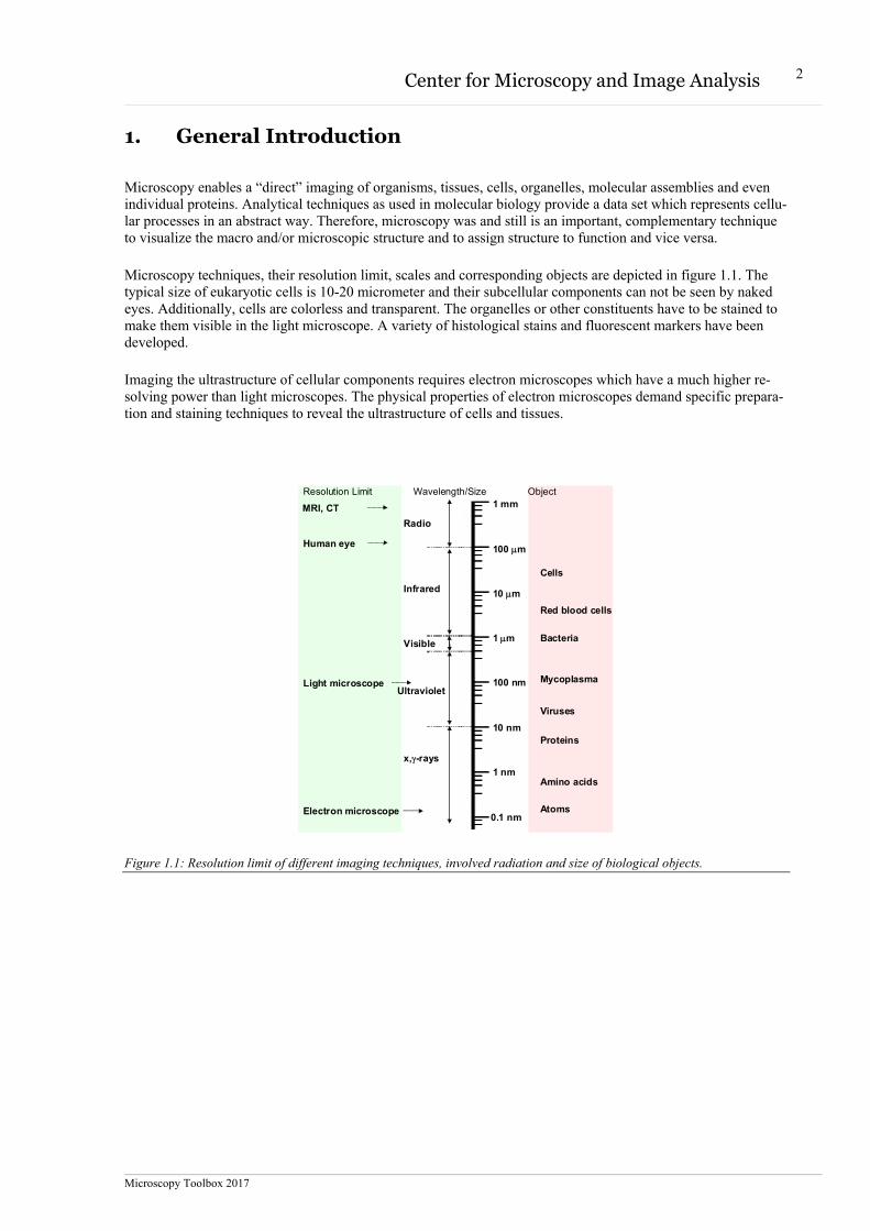
Microscopy techniques, their resolution limit, scales and corresponding objects are depicted in figure 1.1. The typical size of eukaryotic cells is 10-20 micrometer and their subcellular components can not be seen by naked eyes. Additionally, cells are colorless and transparent. The organelles or other constituents have to be stained to make them visible in the light microscope. A variety of histological stains and fluorescent markers have been developed.

Imaging the ultrastructure of cellular components requires electron microscopes which have a much higher re-solving power than light microscopes. The physical properties of electron microscopes demand specific prepara-tion and staining techniques to reveal the ultrastructure of cells and tissues.

Figure 1.1: Resolution limit of different imaging techniques, involved radiation and size of biological objects.

Atoms

1 mm

100 m

10 m

1 m

100 nm

10 nm

1 nm

0.1 nm

Cells

Red blood cells

Bacteria

Mycoplasma

Viruses

Proteins

Amino acids

Radio

Infrared

Visible

Ultraviolet

x,-rays

Human eye

Electron microscope

Light microscope

Resolution Limit Wavelength/Size Object

MRI, CT



2. Light microscopy

As mentioned above, light microscopes use light to illuminate an object and to generate an image of it via objec-tives. This has not been changed since a few hundred years. However, advances in science and technology have profoundly changed light microscopy over the past ten to twenty years. Below is a summary of the bare essen-tials in theory of light microscopy which is intended to allow a better understanding of the demonstrations in the course ‘Microscopy Toolbox’ and as a basic knowledge to stimulate further efforts in understanding micro-scopes. Understanding microscopy and the use of the instrumentation in microscopy is one step towards success-ful research using microscopic techniques.

How is an image formed in a microscope

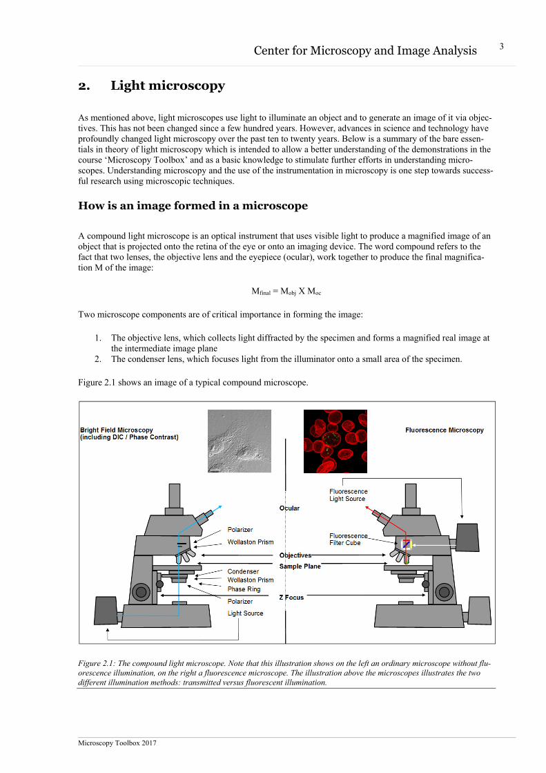
A compound light microscope is an optical instrument that uses visible light to produce a magnified image of an object that is projected onto the retina of the eye or onto an imaging device. The word compound refers to the fact that two lenses, the objective lens and the eyepiece (ocular), work together to produce the final magnifica-tion M of the image:

Mfinal = Mobj X Moc

Two microscope components are of critical importance in forming the image:

1. The objective lens, which collects light diffracted by the specimen and forms a magnified real image at the intermediate image plane

2. The condenser lens, which focuses light from the illuminator onto a small area of the specimen.

Figure 2.1 shows an image of a typical compound microscope.

Figure 2.1: The compound light microscope. Note that this illustration shows on the left an ordinary microscope without flu-orescence illumination, on the right a fluorescence microscope. The illustration above the microscopes illustrates the two different illumination methods: transmitted versus fluorescent illumination.



Figure 2.1 shows an upright microscope design. Inverted microscopes are rapidly gaining in popularity because it is possible to examine living cells in culture dishes filled with medium using standard objectives and avoid the use of sealed flow chambers, which can be awkward. There is also a better access to the stage.

Light as a probe of matter

It is useful to think of light as a probe that can be used to determine the structure of objects viewed under the mi-croscope. Generally, the probes must have size dimensions that are similar to or smaller than the structures being examined (note: compare the probe size and resolution of electron microscopes). As an approximation, the reso-lution limit of the light microscope with an oil immersion objective is about one-half of the wavelength of the light employed.

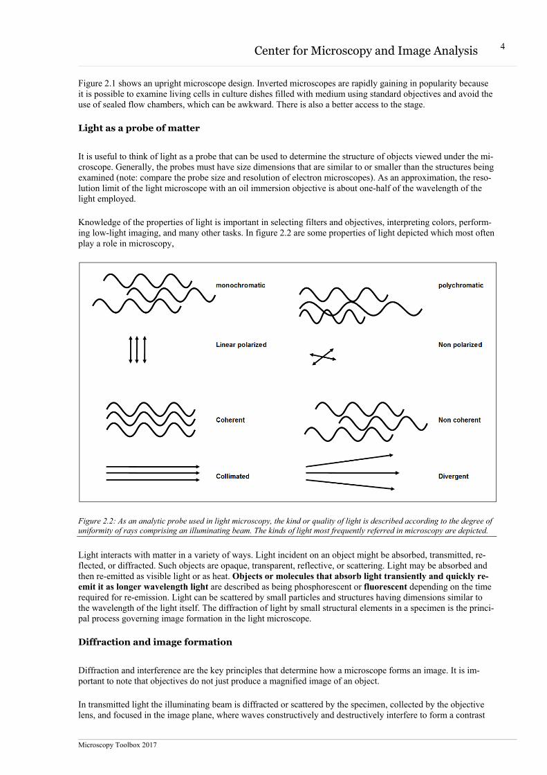
Knowledge of the properties of light is important in selecting filters and objectives, interpreting colors, perform-ing low-light imaging, and many other tasks. In figure 2.2 are some properties of light depicted which most often play a role in microscopy,

Figure 2.2: As an analytic probe used in light microscopy, the kind or quality of light is described according to the degree of uniformity of rays comprising an illuminating beam. The kinds of light most frequently referred in microscopy are depicted.

Light interacts with matter in a variety of ways. Light incident on an object might be absorbed, transmitted, re-flected, or diffracted. Such objects are opaque, transparent, reflective, or scattering. Light may be absorbed and then re-emitted as visible light or as heat. Objects or molecules that absorb light transiently and quickly re-emit it as longer wavelength light are described as being phosphorescent or fluorescent depending on the time required for re-emission. Light can be scattered by small particles and structures having dimensions similar to the wavelength of the light itself. The diffraction of light by small structural elements in a specimen is the princi-pal process governing image formation in the light microscope.

Diffraction and image formation

Diffraction and interference are the key principles that determine how a microscope forms an image. It is im-portant to note that objectives do not just produce a magnified image of an object.

In transmitted light the illuminating beam is diffracted or scattered by the specimen, collected by the objective lens, and focused in the image plane, where waves constructively and destructively interfere to form a contrast



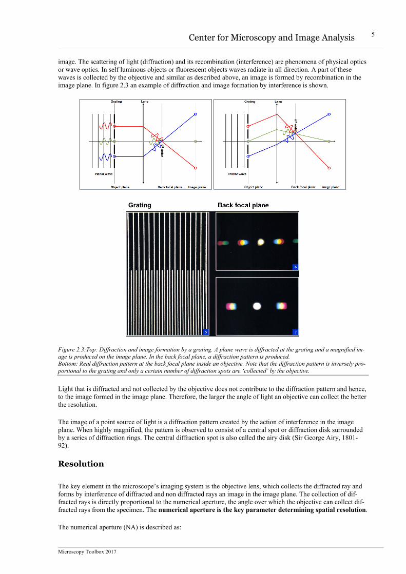
image. The scattering of light (diffraction) and its recombination (interference) are phenomena of physical optics or wave optics. In self luminous objects or fluorescent objects waves radiate in all direction. A part of these waves is collected by the objective and similar as described above, an image is formed by recombination in the image plane. In figure 2.3 an example of diffraction and image formation by interference is shown.

Figure 2.3:Top: Diffraction and image formation by a grating. A plane wave is diffracted at the grating and a magnified im-age is produced on the image plane. In the back focal plane, a diffraction pattern is produced. Bottom: Real diffraction pattern at the back focal plane inside an objective. Note that the diffraction pattern is inversely pro-portional to the grating and only a certain number of diffraction spots are ‘collected’ by the objective.

Light that is diffracted and not collected by the objective does not contribute to the diffraction pattern and hence, to the image formed in the image plane. Therefore, the larger the angle of light an objective can collect the better the resolution.

The image of a point source of light is a diffraction pattern created by the action of interference in the image plane. When highly magnified, the pattern is observed to consist of a central spot or diffraction disk surrounded by a series of diffraction rings. The central diffraction spot is also called the airy disk (Sir George Airy, 1801-92).

Resolution

The key element in the microscope’s imaging system is the objective lens, which collects the diffracted ray and forms by interference of diffracted and non diffracted rays an image in the image plane. The collection of dif-fracted rays is directly proportional to the numerical aperture, the angle over which the objective can collect dif-fracted rays from the specimen. The numerical aperture is the key parameter determining spatial resolution.

The numerical aperture (NA) is described as:

Back focal plane

Grating



NA = n sinα

α is the half angle of the cone of specimen light accepted by the objective lens and n is the refractive index of the medium between the lens and the specimen. For dry lenses used in air, n = 1; for oil immersion objectives, n = 1.515.

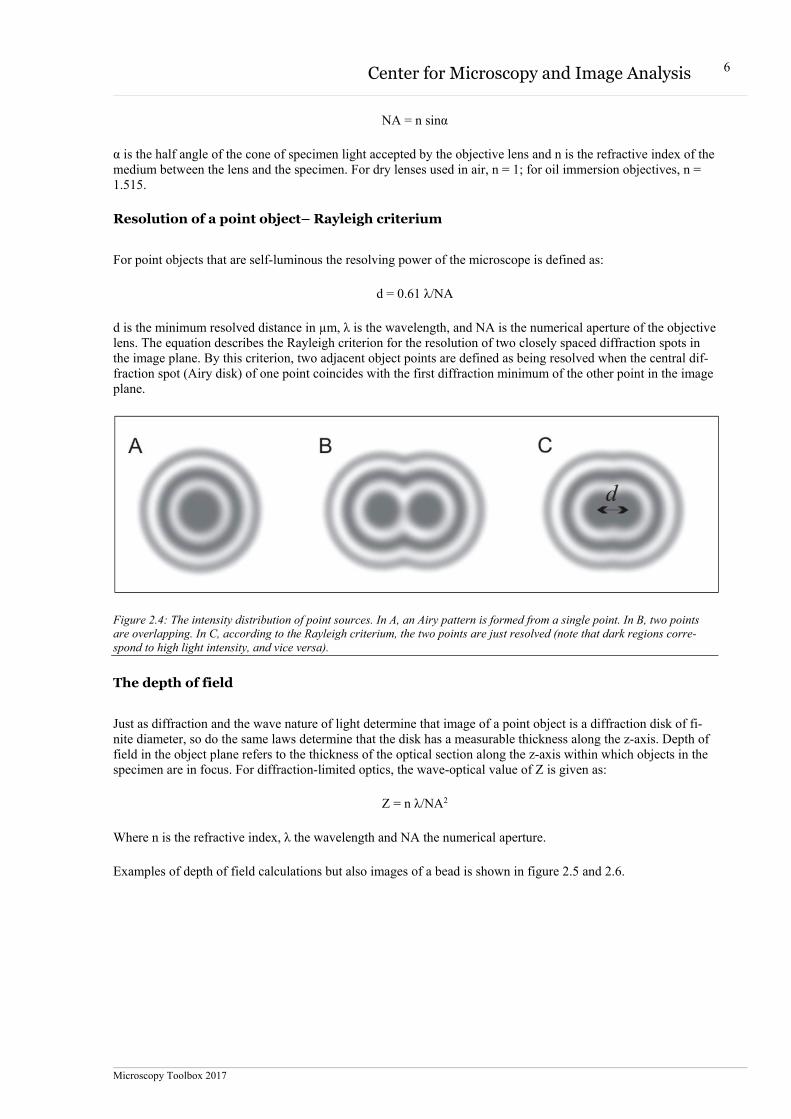
Resolution of a point object– Rayleigh criterium

For point objects that are self-luminous the resolving power of the microscope is defined as:

d = 0.61 λ/NA

d is the minimum resolved distance in µm, λ is the wavelength, and NA is the numerical aperture of the objective lens. The equation describes the Rayleigh criterion for the resolution of two closely spaced diffraction spots in the image plane. By this criterion, two adjacent object points are defined as being resolved when the central dif-fraction spot (Airy disk) of one point coincides with the first diffraction minimum of the other point in the image plane.

Figure 2.4: The intensity distribution of point sources. In A, an Airy pattern is formed from a single point. In B, two points are overlapping. In C, according to the Rayleigh criterium, the two points are just resolved (note that dark regions corre-spond to high light intensity, and vice versa).

The depth of field

Just as diffraction and the wave nature of light determine that image of a point object is a diffraction disk of fi-nite diameter, so do the same laws determine that the disk has a measurable thickness along the z-axis. Depth of field in the object plane refers to the thickness of the optical section along the z-axis within which objects in the specimen are in focus. For diffraction-limited optics, the wave-optical value of Z is given as:

Z = n λ/NA2

Where n is the refractive index, λ the wavelength and NA the numerical aperture.

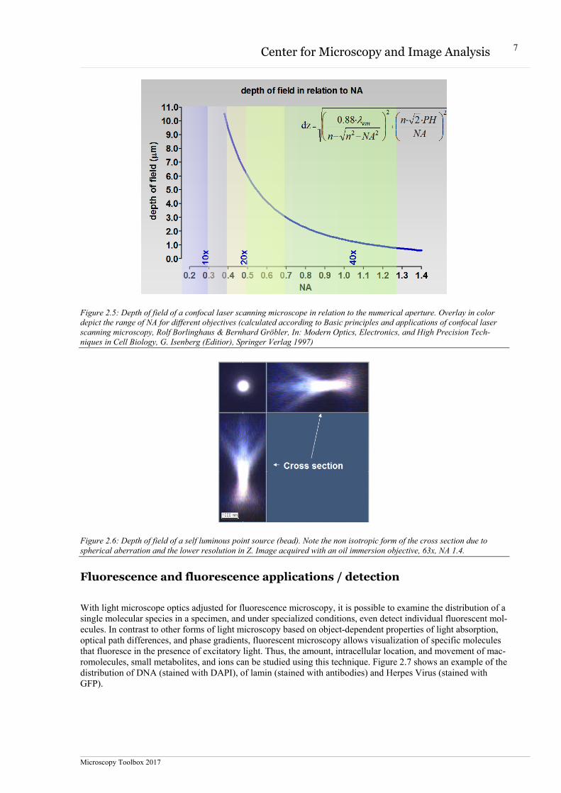
Examples of depth of field calculations but also images of a bead is shown in figure 2.5 and 2.6.



Figure 2.5: Depth of field of a confocal laser scanning microscope in relation to the numerical aperture. Overlay in color depict the range of NA for different objectives (calculated according to Basic principles and applications of confocal laser scanning microscopy, Rolf Borlinghaus & Bernhard Gröbler, In: Modern Optics, Electronics, and High Precision Tech-niques in Cell Biology, G. Isenberg (Editior), Springer Verlag 1997)

Figure 2.6: Depth of field of a self luminous point source (bead). Note the non isotropic form of the cross section due to spherical aberration and the lower resolution in Z. Image acquired with an oil immersion objective, 63x, NA 1.4.

Fluorescence and fluorescence applications / detection

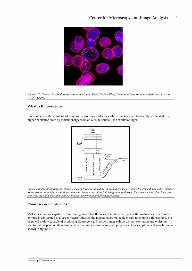
With light microscope optics adjusted for fluorescence microscopy, it is possible to examine the distribution of a single molecular species in a specimen, and under specialized conditions, even detect individual fluorescent mol-ecules. In contrast to other forms of light microscopy based on object-dependent properties of light absorption, optical path differences, and phase gradients, fluorescent microscopy allows visualization of specific molecules that fluoresce in the presence of excitatory light. Thus, the amount, intracellular location, and movement of mac-romolecules, small metabolites, and ions can be studied using this technique. Figure 2.7 shows an example of the distribution of DNA (stained with DAPI), of lamin (stained with antibodies) and Herpes Virus (stained with GFP).



Figure 2.7: Herpes virus in fluorescently stained cells: DNA (DAPI – Blue), lamin (antibody staining – Red), Herpes virus (GFP – Green)

What is fluorescence

Fluorescence is the emission of photons by atoms or molecules whose electrons are transiently stimulated to a higher excitation state by radiant energy from an outside source – the excitation light.

Figure 2.8: Jablonski diagram showing energy levels occupied by an excited electron within a fluorescent molecule. Collapse to the ground state after excitation can occur through any of the following three pathways: fluorescence emission, intersys-tem crossing and generation triplets, internal conversion and phosphorescence.

Fluorescence molecules

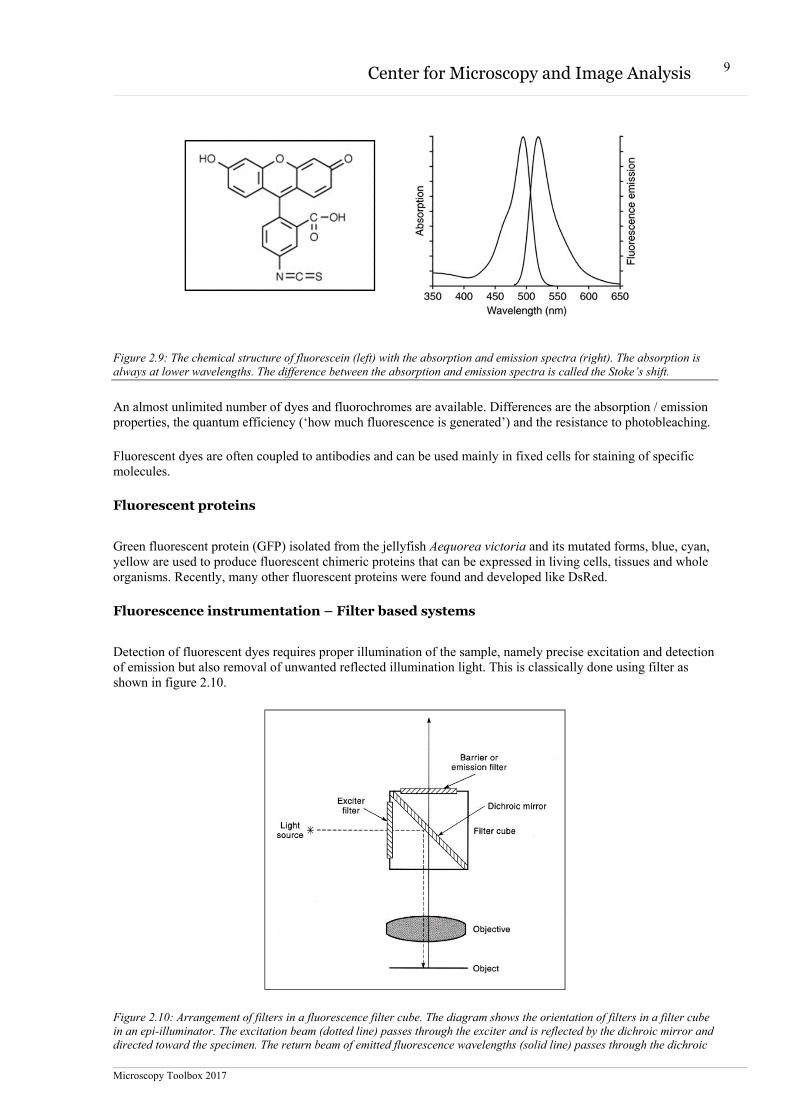
Molecules that are capable of fluorescing are called fluorescent molecules, dyes or fluorochromes. If a fluoro-chrome is conjugated to a larger macromolecule, the tagged macromolecule is said to contain a fluorophore, the chemical moiety capable of producing fluorescence. Fluorochromes exhibit distinct excitation and emission spectra that depend on their atomic structure and electron resonance properties. An example of a fluorochrome is shown in figure 2.9.



Figure 2.9: The chemical structure of fluorescein (left) with the absorption and emission spectra (right). The absorption is always at lower wavelengths. The difference between the absorption and emission spectra is called the Stoke’s shift.

An almost unlimited number of dyes and fluorochromes are available. Differences are the absorption / emission properties, the quantum efficiency (‘how much fluorescence is generated’) and the resistance to photobleaching.

Fluorescent dyes are often coupled to antibodies and can be used mainly in fixed cells for staining of specific molecules.

Fluorescent proteins

Green fluorescent protein (GFP) isolated from the jellyfish Aequorea victoria and its mutated forms, blue, cyan, yellow are used to produce fluorescent chimeric proteins that can be expressed in living cells, tissues and whole organisms. Recently, many other fluorescent proteins were found and developed like DsRed.

Fluorescence instrumentation – Filter based systems

Detection of fluorescent dyes requires proper illumination of the sample, namely precise excitation and detection of emission but also removal of unwanted reflected illumination light. This is classically done using filter as shown in figure 2.10.

Figure 2.10: Arrangement of filters in a fluorescence filter cube. The diagram shows the orientation of filters in a filter cube in an epi-illuminator. The excitation beam (dotted line) passes through the exciter and is reflected by the dichroic mirror and directed toward the specimen. The return beam of emitted fluorescence wavelengths (solid line) passes through the dichroic



mirror and the emission filter. Excitation wavelengths reflected at the specimen are reflected by the dichroic mirror back towards the light source. Excitation wavelengths that manage to pass through the dichroic mirror are blocked by the barrier (emission filter).

Instrumentation

Widefield microscopy

In wide field microscopy the whole sample is illuminated with light. Different modes of illumination can be em-ployed. In transmission microscopy white light is transmitted through stained histological samples. Unstained samples can be analyzed using optical contrast methods (phase contrast, differential interference contrast). Using epiillumination with appropriate filters (see figure 2.10) fluorescent dyes can be excited. Using fluorescent imag-ing in combination with antibody labelling, fluorescent protein expression systems or various dyes, the localiza-tion of numerous molecules as well as physiological processes like Ca2+ concentration, can be measured in high resolution. Wide field microscopy is especially well suited to image living specimens under physiological condi-tions due to a relatively low phototoxicity. Acquisition of images can be in as fast as 25 – 50 frames per second, but also low light imaging is possible with integration times of minutes to detect the faintest signals.

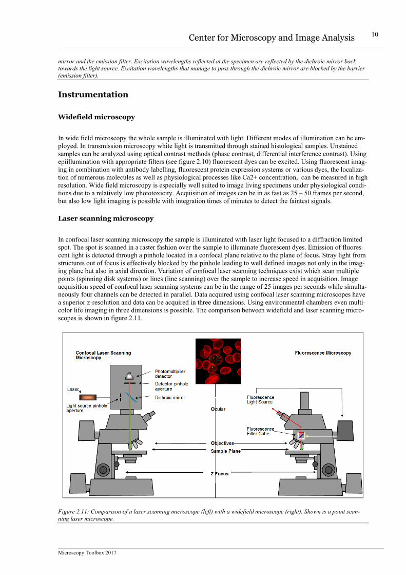
Laser scanning microscopy

In confocal laser scanning microscopy the sample is illuminated with laser light focused to a diffraction limited spot. The spot is scanned in a raster fashion over the sample to illuminate fluorescent dyes. Emission of fluores-cent light is detected through a pinhole located in a confocal plane relative to the plane of focus. Stray light from structures out of focus is effectively blocked by the pinhole leading to well defined images not only in the imag-ing plane but also in axial direction. Variation of confocal laser scanning techniques exist which scan multiple points (spinning disk systems) or lines (line scanning) over the sample to increase speed in acquisition. Image acquisition speed of confocal laser scanning systems can be in the range of 25 images per seconds while simulta-neously four channels can be detected in parallel. Data acquired using confocal laser scanning microscopes have a superior z-resolution and data can be acquired in three dimensions. Using environmental chambers even multi-color life imaging in three dimensions is possible. The comparison between widefield and laser scanning micro-scopes is shown in figure 2.11.

Figure 2.11: Comparison of a laser scanning microscope (left) with a widefield microscope (right). Shown is a point scan-ning laser microscope.



Detection systems

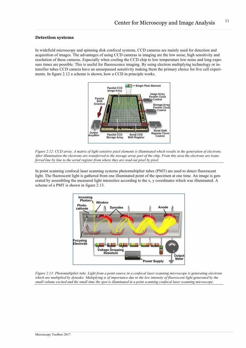
In widefield microscopy and spinning disk confocal systems, CCD cameras are mainly used for detection and acquisition of images. The advantages of using CCD cameras in imaging are the low noise, high sensitivity and resolution of these cameras. Especially when cooling the CCD chip to low temperature low noise and long expo-sure times are possible. This is useful for fluorescence imaging. By using electron multiplying technology or in-tensifier tubes CCD camera have an unsurpassed sensitivity making them the primary choice for live cell experi-ments. In figure 2.12 a scheme is shown, how a CCD in principle works.

Figure 2.12: CCD array. A matrix of light sensitive pixel elements is illuminated which results in the generation of electrons. After illumination the electrons are transferred to the storage array part of the chip. From this area the electrons are trans-ferred line by line to the serial register from where they are read out pixel by pixel.

In point scanning confocal laser scanning systems photomultiplier tubes (PMT) are used to detect fluorescent light. The fluorescent light is gathered from one illuminated point of the specimen at one time. An image is gen-erated by assembling the measured light intensities according to the x, y coordinates which was illuminated. A scheme of a PMT is shown in figure 2.13.

Figure 2.13: Photomultiplier tube. Light from a point source in a confocal laser scanning microscope is generating electrons which are multiplied by dynodes. Multiplying is of importance due to the low intensity of fluorescent light generated by the small volume excited and the small time the spot is illuminated in a point scanning confocal laser scanning microscope.



Special light microscopy applications

Fluorescence after photobleaching

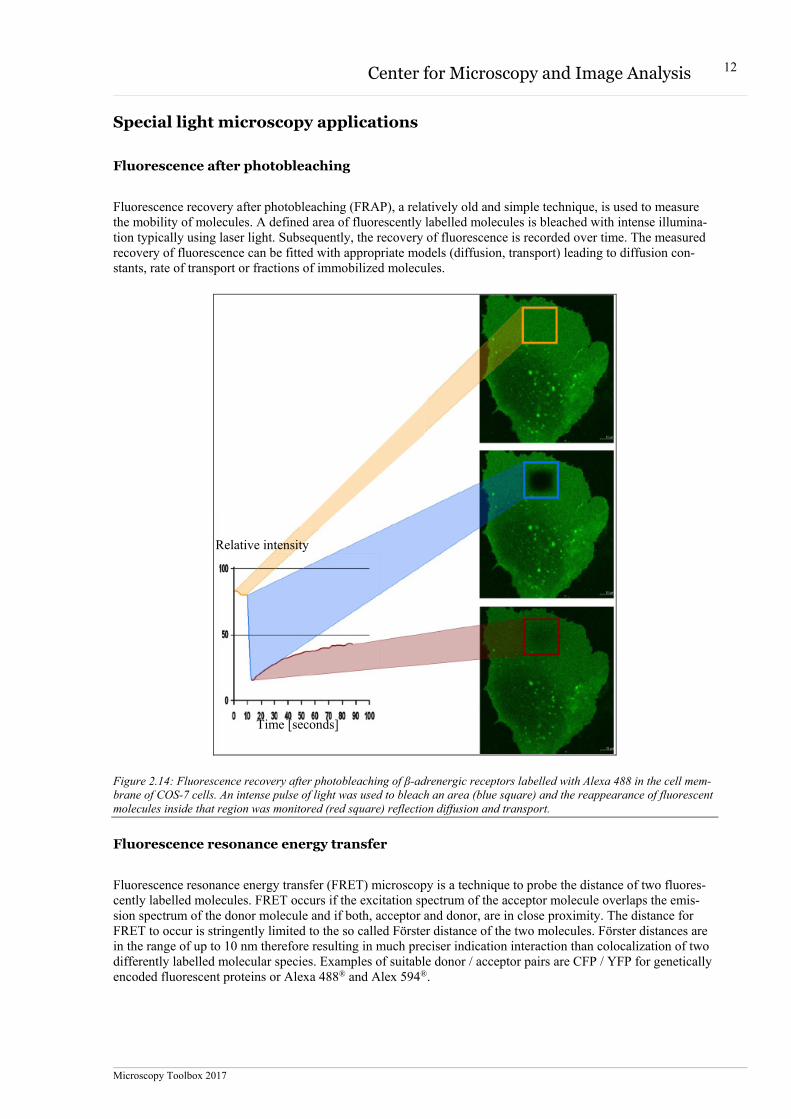
Fluorescence recovery after photobleaching (FRAP), a relatively old and simple technique, is used to measure the mobility of molecules. A defined area of fluorescently labelled molecules is bleached with intense illumina-tion typically using laser light. Subsequently, the recovery of fluorescence is recorded over time. The measured recovery of fluorescence can be fitted with appropriate models (diffusion, transport) leading to diffusion con-stants, rate of transport or fractions of immobilized molecules.

Figure 2.14: Fluorescence recovery after photobleaching of β-adrenergic receptors labelled with Alexa 488 in the cell mem-brane of COS-7 cells. An intense pulse of light was used to bleach an area (blue square) and the reappearance of fluorescent molecules inside that region was monitored (red square) reflection diffusion and transport.

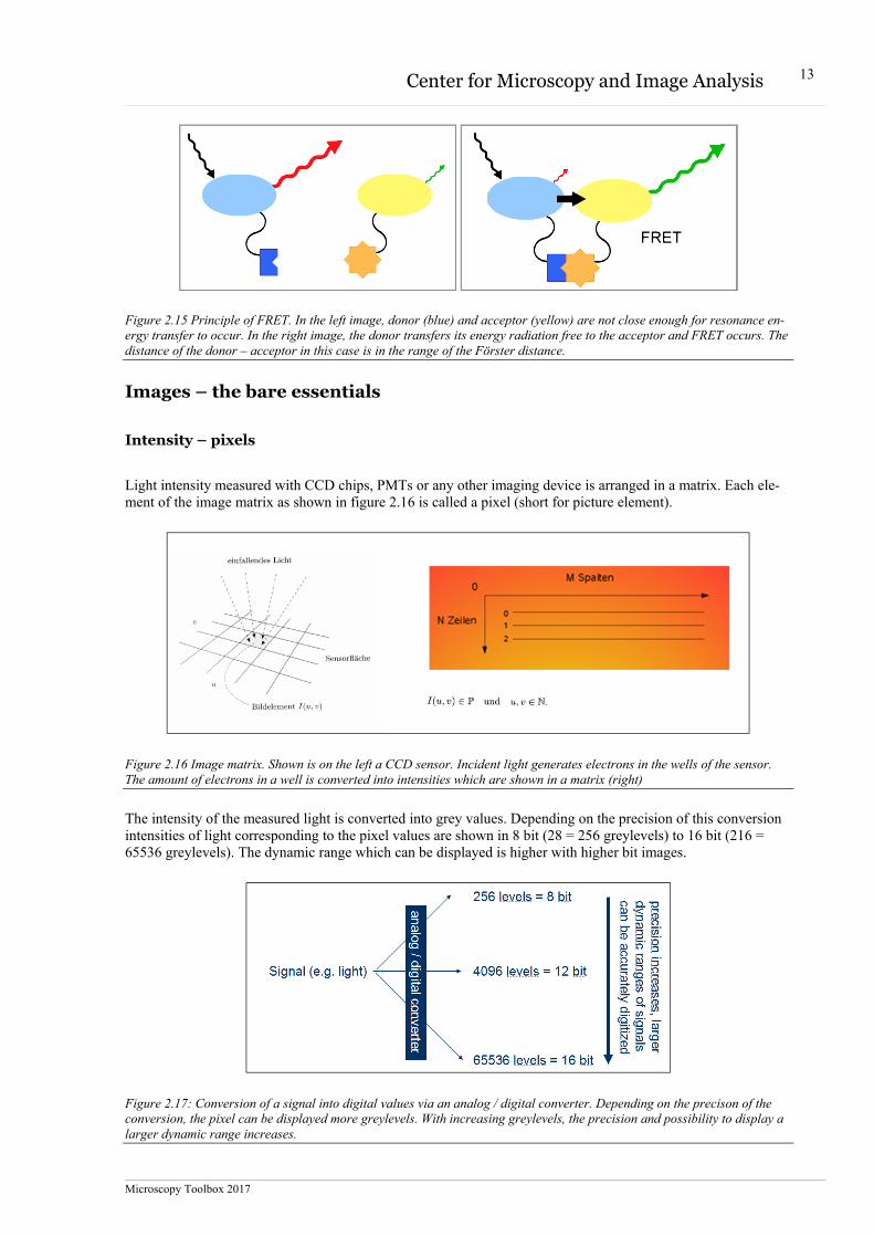
Fluorescence resonance energy transfer

Fluorescence resonance energy transfer (FRET) microscopy is a technique to probe the distance of two fluores-cently labelled molecules. FRET occurs if the excitation spectrum of the acceptor molecule overlaps the emis-sion spectrum of the donor molecule and if both, acceptor and donor, are in close proximity. The distance for FRET to occur is stringently limited to the so called Förster distance of the two molecules. Förster distances are in the range of up to 10 nm therefore resulting in much preciser indication interaction than colocalization of two differently labelled molecular species. Examples of suitable donor / acceptor pairs are CFP / YFP for genetically encoded fluorescent proteins or Alexa 488® and Alex 594®.

Relative intensity

Time [seconds]



Figure 2.15 Principle of FRET. In the left image, donor (blue) and acceptor (yellow) are not close enough for resonance en-ergy transfer to occur. In the right image, the donor transfers its energy radiation free to the acceptor and FRET occurs. The distance of the donor – acceptor in this case is in the range of the Förster distance.

Images – the bare essentials

Intensity – pixels

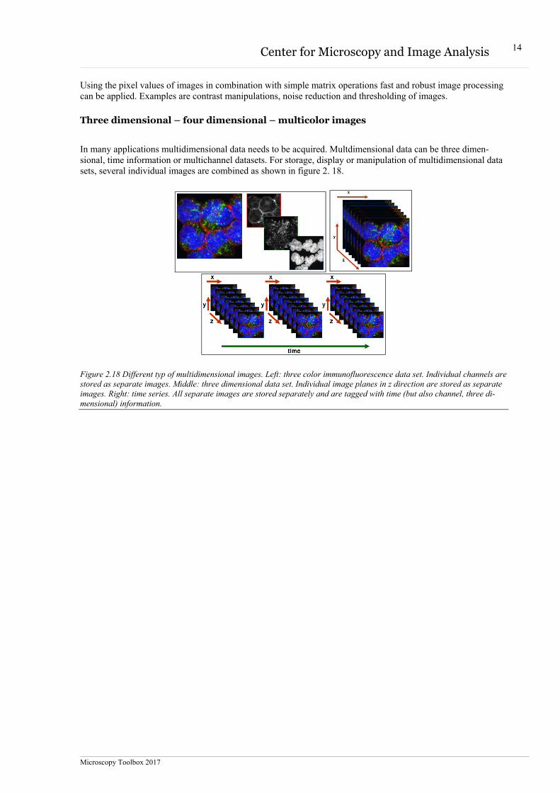
Light intensity measured with CCD chips, PMTs or any other imaging device is arranged in a matrix. Each ele-ment of the image matrix as shown in figure 2.16 is called a pixel (short for picture element).

Figure 2.16 Image matrix. Shown is on the left a CCD sensor. Incident light generates electrons in the wells of the sensor. The amount of electrons in a well is converted into intensities which are shown in a matrix (right)

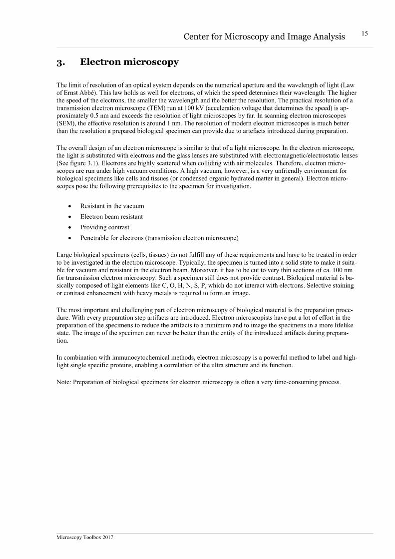
The intensity of the measured light is converted into grey values. Depending on the precision of this conversion intensities of light corresponding to the pixel values are shown in 8 bit (28 = 256 greylevels) to 16 bit (216 = 65536 greylevels). The dynamic range which can be displayed is higher with higher bit images.

Figure 2.17: Conversion of a signal into digital values via an analog / digital converter. Depending on the precison of the conversion, the pixel can be displayed more greylevels. With increasing greylevels, the precision and possibility to display a larger dynamic range increases.



Using the pixel values of images in combination with simple matrix operations fast and robust image processing can be applied. Examples are contrast manipulations, noise reduction and thresholding of images.

Three dimensional – four dimensional – multicolor images

In many applications multidimensional data needs to be acquired. Multdimensional data can be three dimen-sional, time information or multichannel datasets. For storage, display or manipulation of multidimensional data sets, several individual images are combined as shown in figure 2. 18.

Figure 2.18 Different typ of multidimensional images. Left: three color immunofluorescence data set. Individual channels are stored as separate images. Middle: three dimensional data set. Individual image planes in z direction are stored as separate images. Right: time series. All separate images are stored separately and are tagged with time (but also channel, three di-mensional) information.



3. Electron microscopy

The limit of resolution of an optical system depends on the numerical aperture and the wavelength of light (Law of Ernst Abbé). This law holds as well for electrons, of which the speed determines their wavelength: The higher the speed of the electrons, the smaller the wavelength and the better the resolution. The practical resolution of a transmission electron microscope (TEM) run at 100 kV (acceleration voltage that determines the speed) is ap-proximately 0.5 nm and exceeds the resolution of light microscopes by far. In scanning electron microscopes (SEM), the effective resolution is around 1 nm. The resolution of modern electron microscopes is much better than the resolution a prepared biological specimen can provide due to artefacts introduced during preparation.

The overall design of an electron microscope is similar to that of a light microscope. In the electron microscope, the light is substituted with electrons and the glass lenses are substituted with electromagnetic/electrostatic lenses (See figure 3.1). Electrons are highly scattered when colliding with air molecules. Therefore, electron micro-scopes are run under high vacuum conditions. A high vacuum, however, is a very unfriendly environment for biological specimens like cells and tissues (or condensed organic hydrated matter in general). Electron micro-scopes pose the following prerequisites to the specimen for investigation.

Resistant in the vacuum

Electron beam resistant

Providing contrast

Penetrable for electrons (transmission electron microscope)

Large biological specimens (cells, tissues) do not fulfill any of these requirements and have to be treated in order to be investigated in the electron microscope. Typically, the specimen is turned into a solid state to make it suita-ble for vacuum and resistant in the electron beam. Moreover, it has to be cut to very thin sections of ca. 100 nm for transmission electron microscopy. Such a specimen still does not provide contrast. Biological material is ba-sically composed of light elements like C, O, H, N, S, P, which do not interact with electrons. Selective staining or contrast enhancement with heavy metals is required to form an image.

The most important and challenging part of electron microscopy of biological material is the preparation proce-dure. With every preparation step artifacts are introduced. Electron microscopists have put a lot of effort in the preparation of the specimens to reduce the artifacts to a minimum and to image the specimens in a more lifelike state. The image of the specimen can never be better than the entity of the introduced artifacts during prepara-tion.

In combination with immunocytochemical methods, electron microscopy is a powerful method to label and high-light single specific proteins, enabling a correlation of the ultra structure and its function.

Note: Preparation of biological specimens for electron microscopy is often a very time-consuming process.



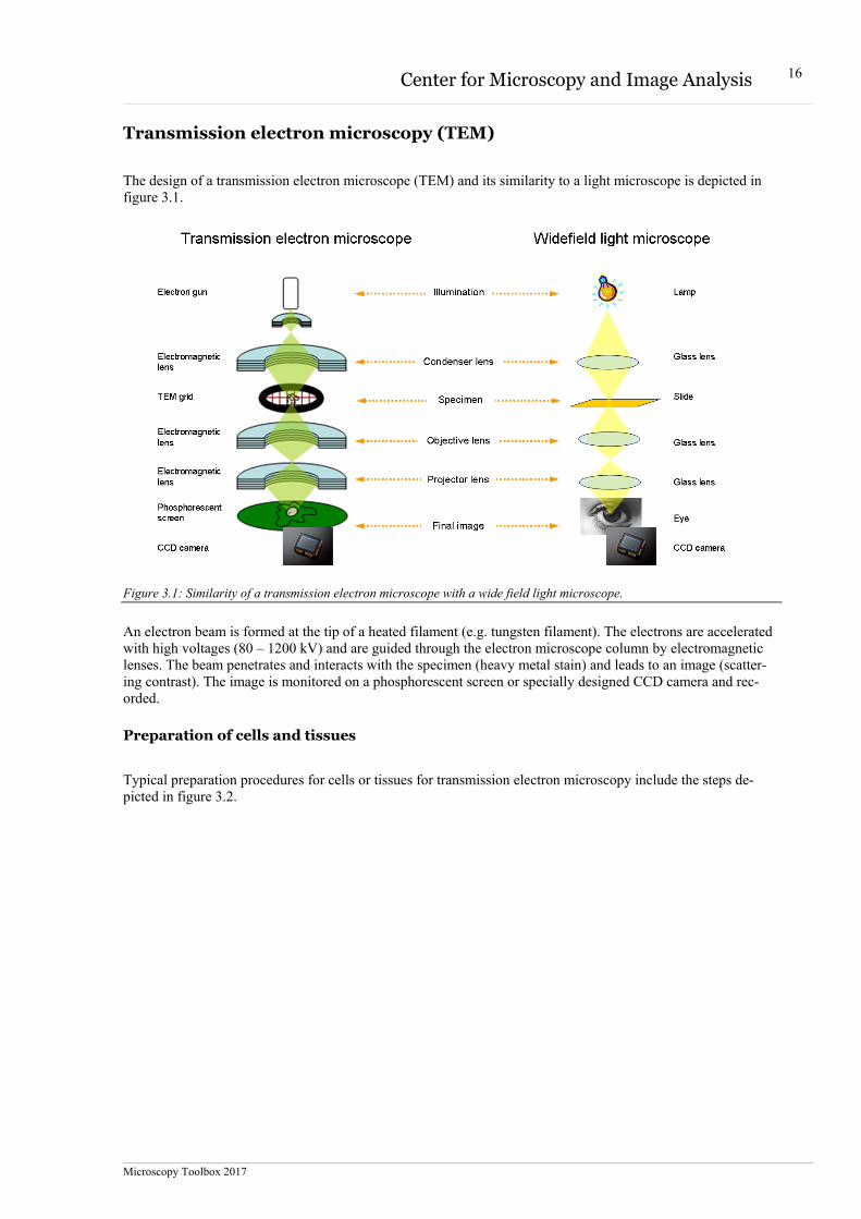
Transmission electron microscopy (TEM)

The design of a transmission electron microscope (TEM) and its similarity to a light microscope is depicted in figure 3.1.

Figure 3.1: Similarity of a transmission electron microscope with a wide field light microscope.

An electron beam is formed at the tip of a heated filament (e.g. tungsten filament). The electrons are accelerated with high voltages (80 – 1200 kV) and are guided through the electron microscope column by electromagnetic lenses. The beam penetrates and interacts with the specimen (heavy metal stain) and leads to an image (scatter-ing contrast). The image is monitored on a phosphorescent screen or specially designed CCD camera and rec-orded.

Preparation of cells and tissues

Typical preparation procedures for cells or tissues for transmission electron microscopy include the steps de-picted in figure 3.2.



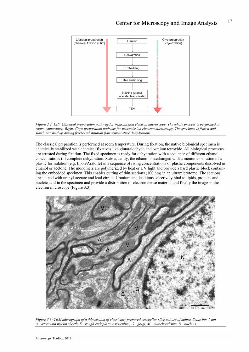
Figure 3.2: Left: Classical preparation pathway for transmission electron microscopy. The whole process is performed at room temperature. Right: Cryo-preparation pathway for transmission electron microscopy. The specimen is frozen and slowly warmed up during freeze-substitution (low temperature dehydration).

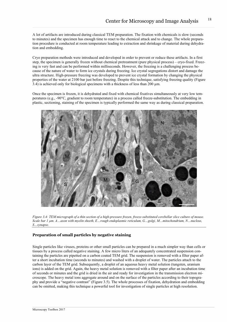
The classical preparation is performed at room temperature. During fixation, the native biological specimen is chemically stabilized with chemical fixatives like glutaraldehyde and osmium tetroxide. All biological processes are arrested during fixation. The fixed specimen is ready for dehydration with a sequence of different ethanol concentrations till complete dehydration. Subsequently, the ethanol is exchanged with a monomer solution of a plastic formulation (e.g. Epon/Araldite) in a sequence of rising concentrations of plastic components dissolved in ethanol or acetone. The monomers are polymerized by heat or UV light and provide a hard plastic block contain-ing the embedded specimen. This enables cutting of thin sections (100 nm) in an ultramicrotome. The sections are stained with uranyl-acetate and lead citrate. Uranium and lead ions selectively bind to lipids, proteins and nucleic acid in the specimen and provide a distribution of electron dense material and finally the image in the electron microscope (Figure 3.3).

Figure 3.3: TEM micrograph of a thin section of classically prepared cerebellar slice culture of mouse. Scale bar 1 µm. A…axon with myelin sheeth, E…rough endoplasmic reticulum, G…golgi, M…mitochondrium, N…nucleus.

Embedding

Fixation

Dehydration

Staining (uranyl-acetate, lead-citrate)

Thin sectioning

TEM

Classical preparation(chemical fixation at RT)

Cryo-preparation(cryo-fixation)

N

G E

A

M

M

M

A

A



A lot of artifacts are introduced during classical TEM preparation. The fixation with chemicals is slow (seconds to minutes) and the specimen has enough time to react to the chemical attack and to change. The whole prepara-tion procedure is conducted at room temperature leading to extraction and shrinkage of material during dehydra-tion and embedding.

Cryo preparation methods were introduced and developed in order to prevent or reduce these artifacts. In a first step, the specimen is generally frozen without chemical pretreatment (pure physical process) – cryo-fixed. Freez-ing is very fast and can be performed within milliseconds. However, the freezing is a challenging process be-cause of the nature of water to form ice crystals during freezing. Ice crystal segregations distort and damage the ultra structure. High-pressure freezing was developed to prevent ice crystal formation by changing the physical properties of the water at 2100 bar just before freezing. Despite this technique, satisfying freezing quality (Figure 3.4) is achieved only for biological specimens with a thickness of less than 200 µm.

Once the specimen is frozen, it is dehydrated and fixed with chemical fixatives simultaneously at very low tem-peratures (e.g., -90°C, gradient to room temperature) in a process called freeze-substitution. The embedding in plastic, sectioning, staining of the specimen is typically performed the same way as during classical preparation.

Figure 3.4: TEM micrograph of a thin section of a high-pressure frozen, freeze-substituted cerebellar slice culture of mouse. Scale bar 1 µm. A…axon with myelin sheeth, E…rough endoplasmic reticulum, G…golgi, M…mitochondrium, N…nucleus, S…synapse.

Preparation of small particles by negative staining

Single particles like viruses, proteins or other small particles can be prepared in a much simpler way than cells or tissues by a process called negative staining. A few micro liters of an adequately concentrated suspension con-taining the particles are pipetted on a carbon coated TEM grid. The suspension is removed with a filter paper af-ter a short incubation time (seconds to minutes) and washed with a droplet of water. The particles attach to the carbon layer of the TEM grid. Subsequently, a droplet of an aqueous heavy metal solution (tungsten, uranium ions) is added on the grid. Again, the heavy metal solution is removed with a filter paper after an incubation time of seconds or minutes and the grid is dried in the air and ready for investigation in the transmission electron mi-croscope. The heavy metal ions aggregate around and on the surface of the particles according to their topogra-phy and provide a “negative contrast” (Figure 3.5). The whole processes of fixation, dehydration and embedding can be omitted, making this technique a powerful tool for investigation of single particles at high resolution.

N

M

M M G G

A

S

E

M



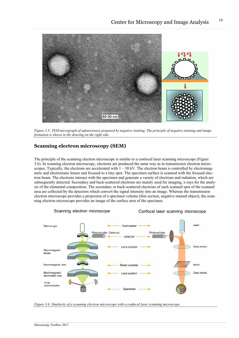
Figure 3.5: TEM micrograph of adenoviruses prepared by negative staining. The principle of negative staining and image formation is shown in the drawing on the right side.

Scanning electron microscopy (SEM)

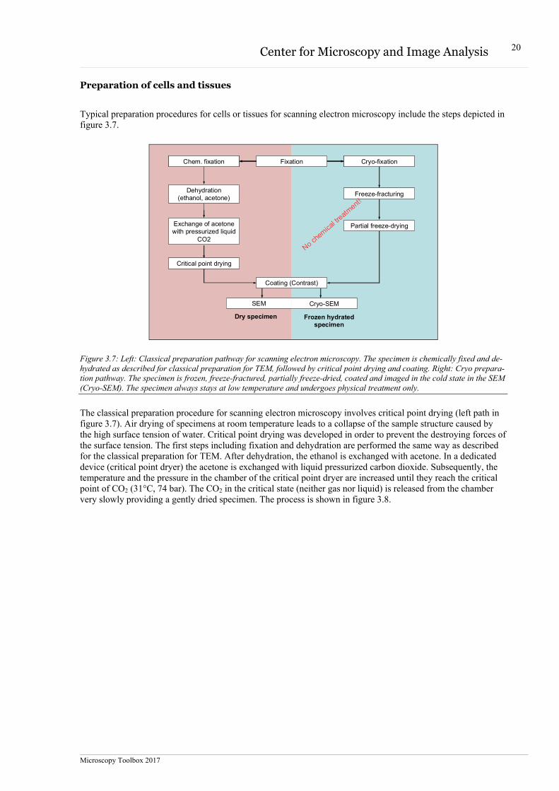
The principle of the scanning electron microscope is similar to a confocal laser scanning microscope (Figure 3.6). In scanning electron microscopy, electrons are produced the same way as in transmission electron micro-scopes. Typically, the electrons are accelerated with 1 – 30 kV. The electron beam is controlled by electromag-netic and electrostatic lenses and focused to a tiny spot. The specimen surface is scanned with the focused elec-tron beam. The electrons interact with the specimen and generate a variety of electrons and radiation, which are subsequently detected. Secondary and back-scattered electrons are mainly used for imaging, x-rays for the analy-sis of the elemental composition. The secondary or back-scattered electrons of each scanned spot of the scanned area are collected by the detectors which convert the signal intensity into an image. Whereas the transmission electron microscope provides a projection of a specimen volume (thin section, negative stained object), the scan-ning electron microscope provides an image of the surface area of the specimen.

Figure 3.6: Similarity of a scanning electron microscope with a confocal laser scanning microscope.



Preparation of cells and tissues

Typical preparation procedures for cells or tissues for scanning electron microscopy include the steps depicted in figure 3.7.

Figure 3.7: Left: Classical preparation pathway for scanning electron microscopy. The specimen is chemically fixed and de-hydrated as described for classical preparation for TEM, followed by critical point drying and coating. Right: Cryo prepara-tion pathway. The specimen is frozen, freeze-fractured, partially freeze-dried, coated and imaged in the cold state in the SEM (Cryo-SEM). The specimen always stays at low temperature and undergoes physical treatment only.

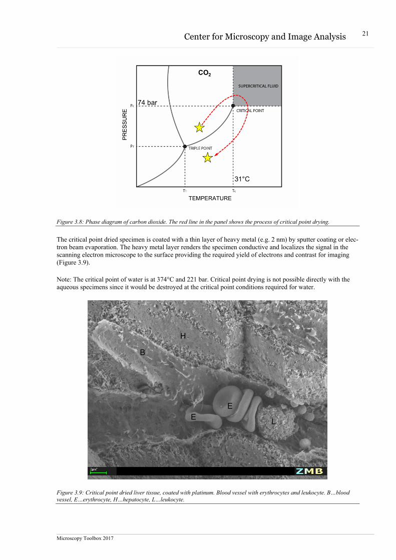
The classical preparation procedure for scanning electron microscopy involves critical point drying (left path in figure 3.7). Air drying of specimens at room temperature leads to a collapse of the sample structure caused by the high surface tension of water. Critical point drying was developed in order to prevent the destroying forces of the surface tension. The first steps including fixation and dehydration are performed the same way as described for the classical preparation for TEM. After dehydration, the ethanol is exchanged with acetone. In a dedicated device (critical point dryer) the acetone is exchanged with liquid pressurized carbon dioxide. Subsequently, the temperature and the pressure in the chamber of the critical point dryer are increased until they reach the critical point of CO2 (31°C, 74 bar). The CO2 in the critical state (neither gas nor liquid) is released from the chamber very slowly providing a gently dried specimen. The process is shown in figure 3.8.

Fixation

Exchange of acetone with pressurized liquid

CO2

Dehydration(ethanol, acetone)

Critical point drying

Chem. fixationChem. fixation Cryo-fixationCryo-fixation

Coating (Contrast)

SEM

Dry specimen

Partial freeze-drying

Freeze-fracturing

Frozen hydrated specimen

Cryo-SEM

No che

mical tr

eatment!



Figure 3.8: Phase diagram of carbon dioxide. The red line in the panel shows the process of critical point drying.

The critical point dried specimen is coated with a thin layer of heavy metal (e.g. 2 nm) by sputter coating or elec-tron beam evaporation. The heavy metal layer renders the specimen conductive and localizes the signal in the scanning electron microscope to the surface providing the required yield of electrons and contrast for imaging (Figure 3.9).

Note: The critical point of water is at 374°C and 221 bar. Critical point drying is not possible directly with the aqueous specimens since it would be destroyed at the critical point conditions required for water.

Figure 3.9: Critical point dried liver tissue, coated with platinum. Blood vessel with erythrocytes and leukocyte. B…blood vessel, E…erythrocyte, H…hepatocyte, L…leukocyte.

H

B

E E

L



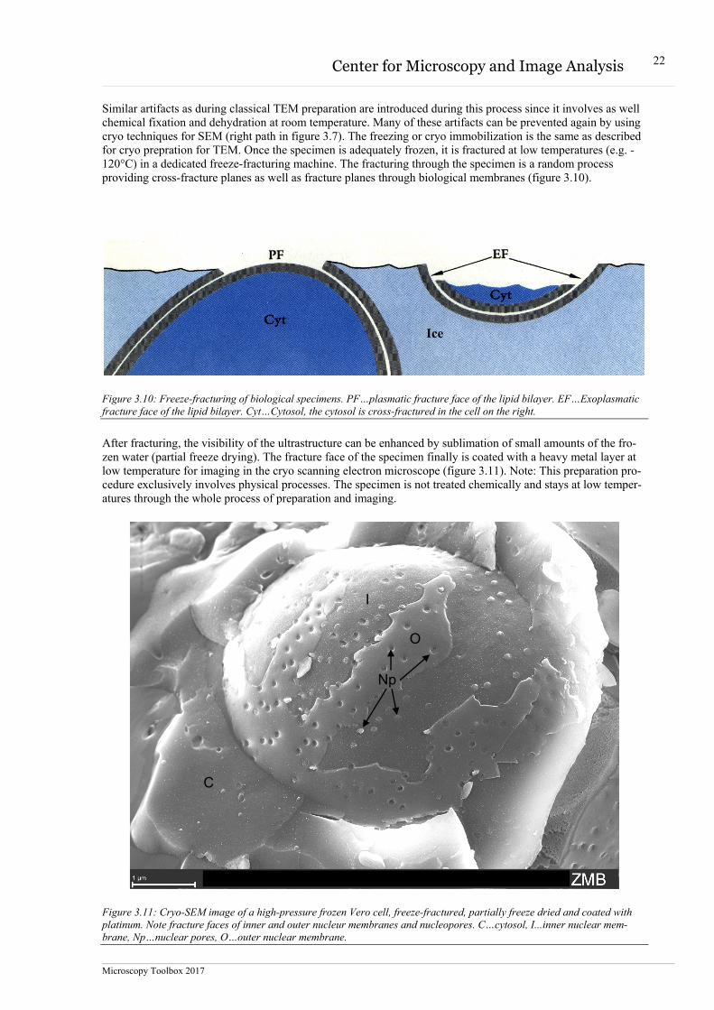
Similar artifacts as during classical TEM preparation are introduced during this process since it involves as well chemical fixation and dehydration at room temperature. Many of these artifacts can be prevented again by using cryo techniques for SEM (right path in figure 3.7). The freezing or cryo immobilization is the same as described for cryo prepration for TEM. Once the specimen is adequately frozen, it is fractured at low temperatures (e.g. -120°C) in a dedicated freeze-fracturing machine. The fracturing through the specimen is a random process providing cross-fracture planes as well as fracture planes through biological membranes (figure 3.10).

Figure 3.10: Freeze-fracturing of biological specimens. PF…plasmatic fracture face of the lipid bilayer. EF…Exoplasmatic fracture face of the lipid bilayer. Cyt…Cytosol, the cytosol is cross-fractured in the cell on the right.

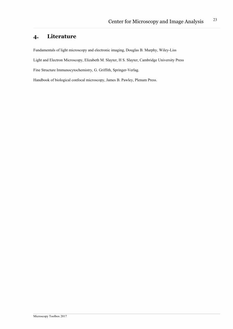
After fracturing, the visibility of the ultrastructure can be enhanced by sublimation of small amounts of the fro-zen water (partial freeze drying). The fracture face of the specimen finally is coated with a heavy metal layer at low temperature for imaging in the cryo scanning electron microscope (figure 3.11). Note: This preparation pro-cedure exclusively involves physical processes. The specimen is not treated chemically and stays at low temper-atures through the whole process of preparation and imaging.

Figure 3.11: Cryo-SEM image of a high-pressure frozen Vero cell, freeze-fractured, partially freeze dried and coated with platinum. Note fracture faces of inner and outer nucleur membranes and nucleopores. C…cytosol, I...inner nuclear mem-brane, Np…nuclear pores, O…outer nuclear membrane.

Ice

I

O

Np

C



4. Literature

Fundamentals of light microscopy and electronic imaging, Douglas B. Murphy, Wiley-Liss

Light and Electron Microscopy, Elizabeth M. Slayter, H S. Slayter, Cambridge University Press

Fine Structure Immunocytochemistry, G. Griffith, Springer-Verlag.

Handbook of biological confocal microscopy, James B. Pawley, Plenum Press.

Documents

A short introduction to light and electron microscopy · 2. Light microscopy As mentioned above, light microscopes use light to illuminate an object and to generate an image of it