Notes on Mathcad

A Short Reference Guide

Hints, Tips and Tricks

Mathcad 2001 Professional

Max R. Knittel

Department of Physics/Astronomy Western Washington University

January 17, 2003

2 Notes on Mathcad

Table of Contents ACKNOWLEDGEMENTS ......................................................................................................................... 4

THE OFFICIAL MATHCAD USER’S GUIDE AND MATHCAD REFERENCE MANUAL ............ 4

NOTATION .................................................................................................................................................. 5

WHAT IS MATHCAD?............................................................................................................................... 5

SAVING ........................................................................................................................................................ 5

THE MATHCAD WORKSPACE .............................................................................................................. 5

ENTERING EQUATIONS IN A MATH REGION .................................................................................. 7

DEFINITIONS AND VARIABLES .................................................................................................................... 7 RANGE VARIABLES..................................................................................................................................... 9 FUNCTIONS ............................................................................................................................................... 11 USE OF ARRAY INDICES ............................................................................................................................ 12 ORDER OF EVALUATION ........................................................................................................................... 15

ENTERING DATA .................................................................................................................................... 16

INPUT LIST................................................................................................................................................ 16 INPUT TABLES........................................................................................................................................... 16

TABLE FORMATTING............................................................................................................................ 18

ENTERING TEXT..................................................................................................................................... 20

UNITS AND DIMENSIONS ..................................................................................................................... 22

PLOTTING................................................................................................................................................. 24

PLOTTING A FUNCTION ............................................................................................................................. 24 PLOTTING TABLES OF DATA ..................................................................................................................... 25 FORMATTING PLOTS ................................................................................................................................. 26

REGRESSION (FITTING A FUNCTION TO DATA) .......................................................................... 27

SYMBOLIC EVALUATION .................................................................................................................... 31

PRINTING.................................................................................................................................................. 33

Notes on Mathcad 3

Acknowledgements Much of the material compiled into this set of notes has come from handouts and lab procedures developed by Drs. Richard Vawter and Rob Quigley. They have made major contributions toward the understanding and use of Mathcad in Physics labs.

The Official Mathcad User’s Guide When logged into a Physics workstation, you can refer to the official Mathcad documentation by selecting Mathcad 2001 User’s Guide from the Physics Applications folder.

4 Notes on Mathcad

Notation Whenever you are to type something, the keystrokes will be displayed in bold courier font. You will be asked to:

You type: v.initial:a^2[space]+b^2 Mathcad shows on the screen: vinitial := a2 + b2

What is Mathcad? Mathcad is a calculation, graphing and presentation computer application. Mathcad displays equations as you are used to seeing them in text books and lets you insert graphs and text as you build your document. It is a powerful tool for writing laboratory reports, letting you write introductions, conclusions, and enter (or import) experimental data, analyze the data, and then graph your results and fit theoretical functions to the experimental points. You can also solve just about any mathematical problem, symbolically or numerically.

Saving You may think it odd to discuss saving your Mathcad worksheet in one of the first sections of this reference guide, but Mathcad is not a forgiving application. Mathcad will not let you undo a number of operations, as you may be used to in other applications. For example, if you accidentally delete the wrong region, you cannot get it back! So make sure you save early and often so you don’t have to manually redo much work if you perform some operation you wish you hadn’t. Additionally, Mathcad crashes on occasion (actually, quite often for a program as mature as Mathcad). Before performing any radical operation such as moving a lot of regions or printing, save your work. It doesn’t hurt to even have two copies of your work: one in your U:\ home directory and one on a floppy diskette or Zip disk.

The Mathcad Workspace When you start Mathcad, you’ll see a window with some familiar toolbars. The top line of the window is the familiar Windows File Edit … menu headings. The next line is the Standard toolbar with icons for File, Print, Print Preview, Cut and Paste, etc. The third line is the Formatting toolbar for font type, size and attributes. A floating Math toolbar accompanies the Mathcad window. Clicking on an icon in the Math toolbar opens other toolbars:

• Calculator—Common arithmetic operators

Notes on Mathcad 5

• Graph—Various two- and three-dimensional plot types and graph tools.

• Matrix—Matrix and vector operators

• Evaluation—Equal signs for evaluation and definition

• Calculus—Derivatives, integrals, limits, and iterated sums and products

• Boolean—Comparative and logical operators for Boolean expression

• Programming—Programming constructs

• Greek—Greek letters

• Symbolic—Symbolic keywords

Mathcad lets you enter equations and text anywhere on the page. Each equation, piece of text, or other element is a region. Mathcad creates an invisible rectangle to hold each region. A Mathcad worksheet is a collection of these regions. To start a new region, click anywhere in a blank area of a page. You will see a small crosshair cursor at this point; anything you now type appears at the crosshair. If you want to create a math region at this point, just start typing. If you want to create a text region at this point, first select Insert/Text Region from the top of the Mathcad workspace, and then start typing. To select a single text region, simply click anywhere in it. Mathcad shows a rectangle around the region. To select multiple regions, click and hold at one corner and drag the selection box to the other corner until all desired regions are displayed inside dashed rectangles. You can also use the standard windows techniques of holding down the <Ctrl> key while clicking to add regions one-at-a-time to the selected regions or holding down the <Shift> and clicking on the first and last regions to select all regions in between. After selecting a region, you can drag, delete, cut, copy or paste as with most Windows applications. You can even copy and paste math and plot regions from Mathcad into Microsoft Word.

6 Notes on Mathcad

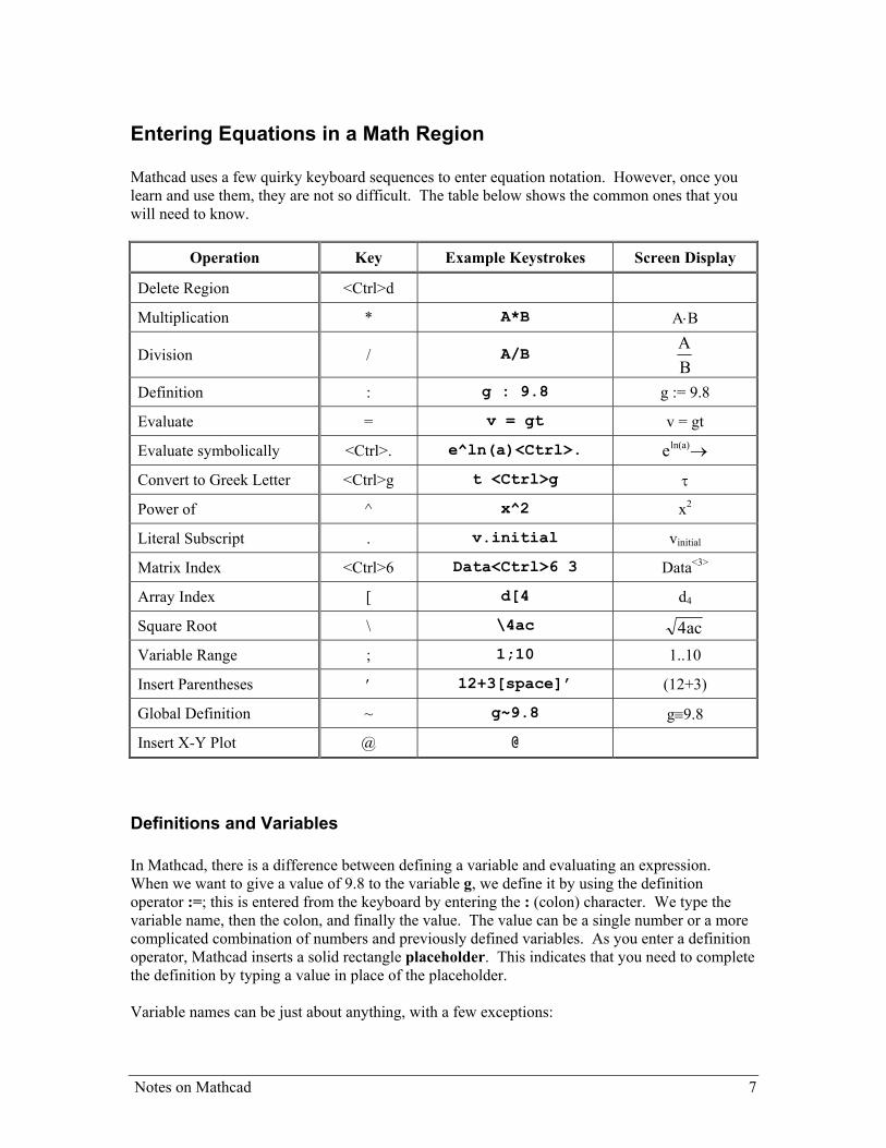
Entering Equations in a Math Region Mathcad uses a few quirky keyboard sequences to enter equation notation. However, once you learn and use them, they are not so difficult. The table below shows the common ones that you will need to know.

Operation Key Example Keystrokes Screen Display

Delete Region <Ctrl>d

Multiplication * A*B A⋅B

Division / A/B AB

Definition : g : 9.8 g := 9.8

Evaluate = v = gt v = gt

Evaluate symbolically <Ctrl>. e^ln(a)<Ctrl>. eln(a)→

Convert to Greek Letter <Ctrl>g t <Ctrl>g τ

Power of ^ x^2 x2

Literal Subscript . v.initial vinitial

Matrix Index <Ctrl>6 Data<Ctrl>6 3 Data<3>

Array Index [ d[4 d4

Square Root \ \4ac 4ac

Variable Range ; 1;10 1..10

Insert Parentheses ′ 12+3[space]’ (12+3)

Global Definition ~ g~9.8 g≡9.8

Insert X-Y Plot @ @

Definitions and Variables In Mathcad, there is a difference between defining a variable and evaluating an expression. When we want to give a value of 9.8 to the variable g, we define it by using the definition operator :=; this is entered from the keyboard by entering the : (colon) character. We type the variable name, then the colon, and finally the value. The value can be a single number or a more complicated combination of numbers and previously defined variables. As you enter a definition operator, Mathcad inserts a solid rectangle placeholder. This indicates that you need to complete the definition by typing a value in place of the placeholder. Variable names can be just about anything, with a few exceptions:

Notes on Mathcad 7

• Names cannot start with a digit (0 – 9). • Names can contain uppercase and lowercase letters, digits, Greek letters, literal

subscripts that are entered starting with a . (period). • An uppercase character is interpreted as a different character from its lowercase

counterpart; e.g., DIAM is a different variable name than diam or diaM. Greek letters can be selected from the Greek toolbar or by typing the the normal keyboard equivalent of the Greek letter and then immediately typing <Ctrl>g. For example, typing t <Ctrl>g yields τ, p<Ctrl>g yields π. Names with literal subscripts (“literal” meaning that Mathcad is to take the subscript just as the characters appear) are different than a name with an array index subscript. The literal subscript is merely an extension of the variable name, while an array index indicates which one of an array is to be used. The array index subscript is entered by typing the variable name, then the character [ (left square bracket), and finally the array index—which could be a number or another variable name (x1, vj).

• Mathcad has a number of built in functions, constants and units such as sin, g, π, e,

etc. You can redefine these if you wish. To evaluate an expression, you enter the “=” character. For example, if you have defined g to be 9.8, t to be 10, and d to be 1/2gt2, then to evaluate the distance d you would type: g:9.8 Define the variable g t:10 Define the variable t d:1/2[space]*g*t^2 Define the variable d d= Evaluate d The value for d is evaluated and displayed automatically after you type the “=” sign. In the definition above for d, the keyboard strokes indicates that a [space] should be typed after “1/2”. This is to move the insertion point from the denominator of the fraction back up to the main line of the expression. The use of the spacebar in a math region is to cycle through what portion of the math region is currently selected. When entering characters into a math region, two editing lines replace the crosshair cursor to show you where the insertion point will be. The vertical editing line shows where the next character you type will appear, while the horizontal editing line indicates at what level the next character will appear. Pressing the spacebar when in a math region cycles the insertion point around to the various possible levels in the region. For another example, you may want to set the first 0th element of a velocity table equal to the initial velocity vinitial. v.initial:9.8 Define the variable vinitial using a literal subscript

8 Notes on Mathcad

v[0:v.initial Define the 0th element of the v array using an array index to be vinitial using a literal subscript

If you want to insert parentheses to set the precedence of operations, make sure that the two editing lines encompass the part of the expression you want to enclose in parentheses and then press the “’” (single quote) key or select Parentheses from the Calculator toolbar. For example, in the definition above for d, pressing the spacebar will in turn select the whole expression, the numerator of the fraction, the denominator of the fraction, and then the whole ½. This enables you to select what portion of the expression to edit. Using the mouse to move the editing lines to the superscript 2 will then let you use the spacebar to cycle through selecting the various points of that part of the expression. The use of the mouse and the spacebar lets you place the editing lines at exactly the point you want to edit.

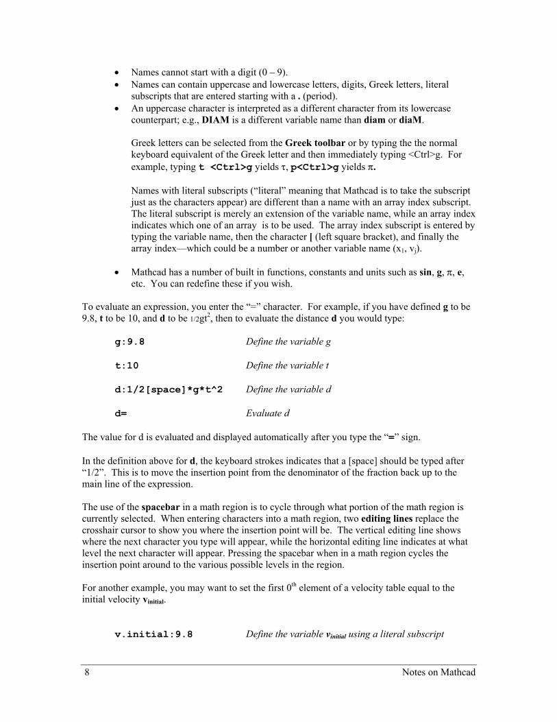
Range Variables To compute equations for a range of values, you first create a range variable. A range variable is defined in the normal way any variable is defined: you type the name and a : (colon). In the placeholder rectangle, instead of entering a single value, you enter the first value, a comma, the second value, a ; (semi-colon)—which shows in the worksheet as two dots—and then the last value. You may be more familiar with entering ranges with first value, last value and interval, but Mathcad calculates the interval from the difference between the first and second values. If the interval value is to be 1, then you can omit the second value and merely type the first value, semicolon, and last value. Once you define a range variable, it takes on its complete range of values every time you use it. If you use a range variable in an equation, Mathcad evaluates that equation for each value of the range variable. For example, to create a range variable t that takes on the values from 1 to 21 with an interval of 2, you would type: t:1,3;21 and Mathcad would display: t := 1, 3 .. 21 To see these values, you want to create an output table. If you type t= Mathcad creates a single column output table directly below. By default, the maximum length of the table is 16 rows; if your range variable takes on more than 16 values, click on the output table; it will turn into a scrolling table, and you can use the scroll bar to move down through the rest of the values. You can use a range variable to create a series of values at which to evaluate an indexed variable. For example, if you type f[t:10*t then you can display a vector of all the answers by typing f[t= .

Notes on Mathcad 9

t 1 3, 21..:=

ft 10 t⋅:=

ft

1030

50

70

90

110

130

150

170

190

210

=t13

5

7

9

11

13

15

17

19

21

=

f3 30=

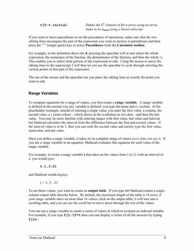
Mathcad will calculate a value for f for each value of t. You can display the fourth element by typing f[3= . Note that using a range variable as an array index only works if all values of the range variable are integers; e.g., you can’t generate the 3.5 element of an array. If you are going to turn in a printed copy of your Mathcad worksheet, you should consider expanding the length of the displayed table so that all of your values will print. If the table will be far too long, you can show it in pieces by typing f[t= several times across the page and setting the scroll bars for the tables to successively lower positions.

ft

0

01

2

3

4

5

1030

50

70

90

110

= ft

0

67

8

9

10

130150

170

190

210

=

Note that to turn on table row and column numbering, right click on it and choose Properties. Place a check mark in the box for Show column/row labels.

10 Notes on Mathcad

Functions Mathcad has an extensive built-in function set. You can define additional functions in the same way you define a variable, except that the function name contains an argument list. The argument list are the variables enclosed in parentheses on the left side of the equals sign. For example, to define the function dist(x,y), where (x,y) is the argument list, you would: Type: dist(x,y):\x^2[space]+y^2

Display: dist(x, y) := x2 + y2

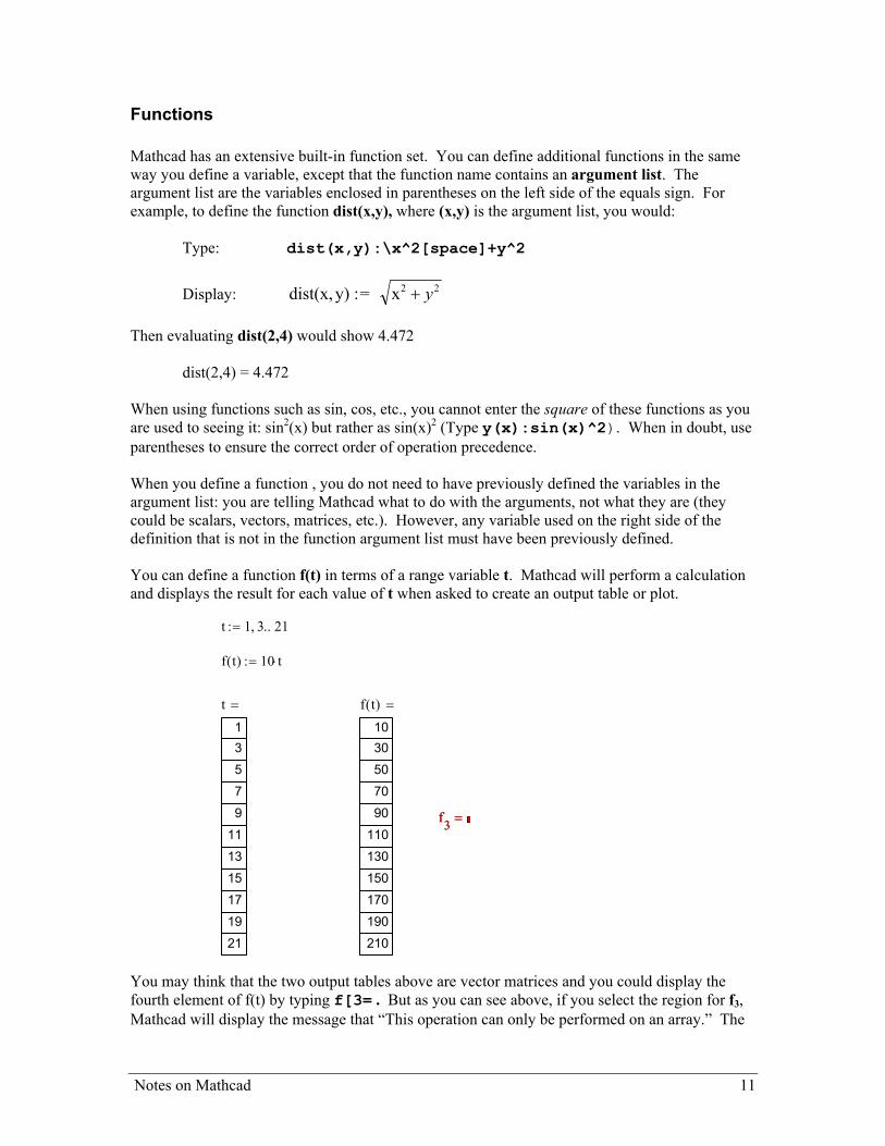
Then evaluating dist(2,4) would show 4.472 dist(2,4) = 4.472 When using functions such as sin, cos, etc., you cannot enter the square of these functions as you are used to seeing it: sin2(x) but rather as sin(x)2 (Type y(x):sin(x)^2). When in doubt, use parentheses to ensure the correct order of operation precedence. When you define a function , you do not need to have previously defined the variables in the argument list: you are telling Mathcad what to do with the arguments, not what they are (they could be scalars, vectors, matrices, etc.). However, any variable used on the right side of the definition that is not in the function argument list must have been previously defined. You can define a function f(t) in terms of a range variable t. Mathcad will perform a calculation and displays the result for each value of t when asked to create an output table or plot.

t 1 3, 21..:=

f t( ) 10 t⋅:=

t13

5

7

9

11

13

15

17

19

21

= f t( )1030

50

70

90

110

130

150

170

190

210

=

f3 =f3 =

You may think that the two output tables above are vector matrices and you could display the fourth element of f(t) by typing f[3= . But as you can see above, if you select the region for f3, Mathcad will display the message that “This operation can only be performed on an array.” The

Notes on Mathcad 11

output table of a function is just a display and the individual elements cannot be addressed and used elsewhere. You could evaluate f(3) and get 30. For the same reason, you cannot omit a range variable from the function argument list, even though it may seem you have already defined the values of t before you defined the function f.

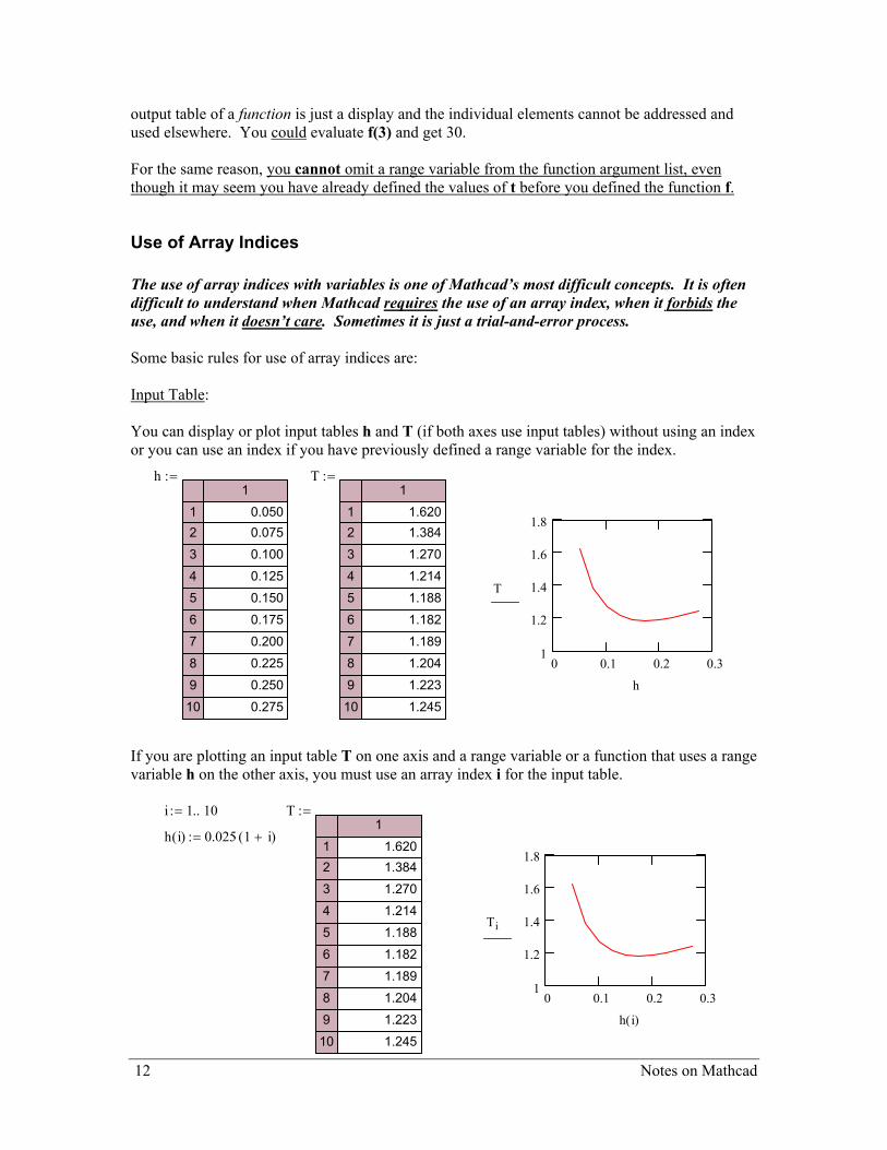
Use of Array Indices The use of array indices with variables is one of Mathcad’s most difficult concepts. It is often difficult to understand when Mathcad requires the use of an array index, when it forbids the use, and when it doesn’t care. Sometimes it is just a trial-and-error process. Some basic rules for use of array indices are: Input Table: You can display or plot input tables h and T (if both axes use input tables) without using an index or you can use an index if you have previously defined a range variable for the index.

h1

12

3

4

5

6

7

8

9

10

0.0500.075

0.100

0.125

0.150

0.175

0.200

0.225

0.250

0.275

:= T1

12

3

4

5

6

7

8

9

10

1.6201.384

1.270

1.214

1.188

1.182

1.189

1.204

1.223

1.245

:=

0 0.1 0.2 0.31

1.2

1.4

1.6

1.8

T

h

If you are plotting an input table T on one axis and a range variable or a function that uses a range variable h on the other axis, you must use an array index i for the input table.

i 1 10..:= T1

12

3

4

5

6

7

8

9

10

1.6201.384

1.270

1.214

1.188

1.182

1.189

1.204

1.223

1.245

:=

h i( ) 0.025 1 i+( )⋅:=

0 0.1 0.2 0.31

1.2

1.4

1.6

1.8

Ti

h i( )

12 Notes on Mathcad

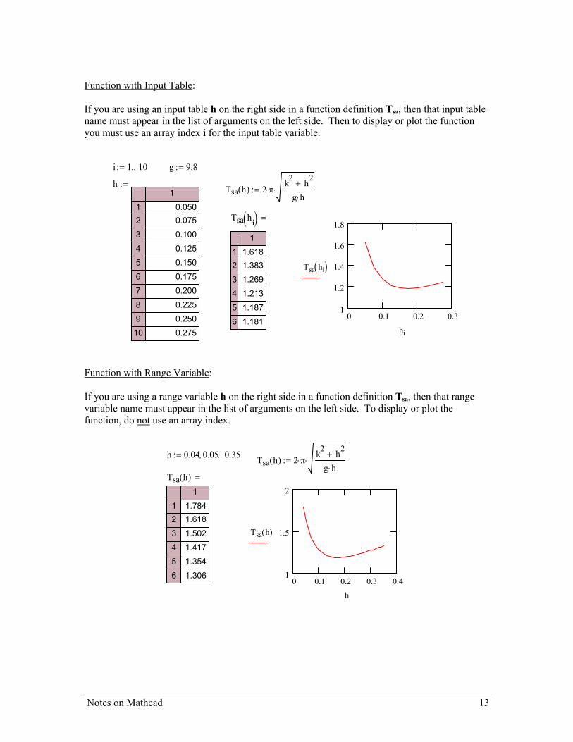
Function with Input Table: If you are using an input table h on the right side in a function definition Tsa, then that input table name must appear in the list of arguments on the left side. Then to display or plot the function you must use an array index i for the input table variable.

i 1 10..:= g 9.8:=

h1

12

3

4

5

6

7

8

9

10

0.0500.075

0.100

0.125

0.150

0.175

0.200

0.225

0.250

0.275

:= Tsa h( ) 2 π⋅k2 h2

+

g h⋅⋅:=

0 0.1 0.2 0.31

1.2

1.4

1.6

1.8

Tsa hi( )

hi

Tsa hi( )1

12

3

4

5

6

1.6181.383

1.269

1.213

1.187

1.181

=

Function with Range Variable: If you are using a range variable h on the right side in a function definition Tsa, then that range variable name must appear in the list of arguments on the left side. To display or plot the function, do not use an array index.

h 0.04 0.05, 0.35..:= Tsa h( ) 2 π⋅k2 h2

+

g h⋅⋅:=

Tsa h( )1

12

3

4

5

6

1.7841.618

1.502

1.417

1.354

1.306

=

0 0.1 0.2 0.3 0.41

1.5

2

Tsa h( )

h

Notes on Mathcad 13

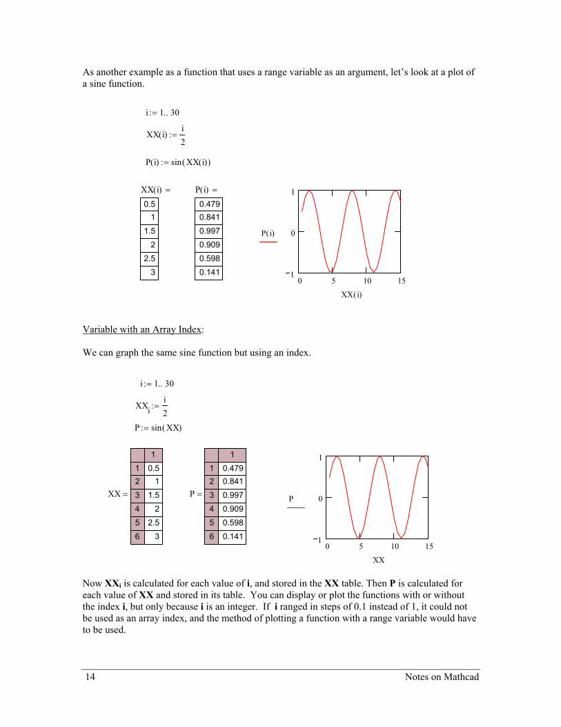
As another example as a function that uses a range variable as an argument, let’s look at a plot of a sine function.

i 1 30..:=

XX i( )i2

:=

P i( ) sin XX i( )( ):=

0 5 10 151

0

1

P i( )

XX i( )

XX i( )0.5

1

1.5

2

2.5

3

= P i( )0.4790.841

0.997

0.909

0.598

0.141

=

Variable with an Array Index: We can graph the same sine function but using an index.

i 1 30..:=

XXii2

:=

P sin XX( ):=

0 5 10 151

0

1

P

XX

XX

1

12

3

4

5

6

0.51

1.5

2

2.5

3

= P

1

12

3

4

5

6

0.4790.841

0.997

0.909

0.598

0.141

=

Now XXi is calculated for each value of i, and stored in the XX table. Then P is calculated for each value of XX and stored in its table. You can display or plot the functions with or without the index i, but only because i is an integer. If i ranged in steps of 0.1 instead of 1, it could not be used as an array index, and the method of plotting a function with a range variable would have to be used.

14 Notes on Mathcad

Order of Evaluation In the above examples, the order and location of the various math regions is very important. Mathcad updates the results of all math regions as soon as you make a change and click outside of the current math region. Mathcad starts at the top left of the document and goes from left to right and top to bottom. Therefore, you must make all of your definitions above or to the left of when they are used. If you try to use a variable before it is defined, it will be highlighted in red; selecting that math region will pop up an error message. Particularly in plotting, what may look like Mathcad telling you there is a serious error is nothing more than the plot is actually above where your X- or Y-axis data is evaluated. You can redefine a variable as often as you like in a worksheet, so be aware that the same name may not have the same value everywhere. It is possible to define a variable whose value is defined even above its location in the worksheet. This is called a global definition. It is done by typing the “~” (tilde) instead of the “:” (colon) in the definition. In the worksheet, it appears as the standard three-bar math definition symbol ≡. If J is globally defined to be 7 (J ≡ 7) at the end of a worksheet, J will be 7 anywhere in the worksheet. Sometimes in editing a Mathcad document, you need to insert space in the middle in order to enter additional definition or text. Use the mouse to position the crosshair cursor at the point you want to insert space and press the <Enter> key as many times as needed.

Notes on Mathcad 15

Entering Data There are a number of ways to enter data into Mathcad. For example, you can type in a list and Mathcad will build a table, you can insert an input table and Mathcad creates a table that looks like a spreadsheet, or you can import data files saved from other applications.

Input List To enter lists of numbers—such as experimental data for analysis or plotting—you can create a table. First define a range variable as an array index. Type: j:1;21 Next define your data variable such as dj and start entering your data values separated by commas. Type: d[j:2.3,5.6,7.9,12.4 Mathcad displays: d j

2.35.67.912.4

:= As soon as you type the first comma, Mathcad changes the expression into a table, adding a new row each time you press the comma. You can go back and insert rows by clicking at the end of a number in the table, hitting the comma key and then typing the next value in the new row. The display of this type of table stays just as you type in the numbers.

Input Tables Alternatively, you can create an Input Table by placing the cursor where you want the table to start and selecting Insert/Component/Input Table. Type a variable name in the placeholder at the top and use the handles on the table to enlarge or shrink it in rows and columns to fit the size of the data you want to enter. Values not entered into the input table are assumed to be zero by Mathcad. You can change the display of an input table by right clicking on a table entry and selecting Properties. You can set the Displayed precision, whether or not to Show trailing zeros, and whether or not to Show column/row labels. Although the global table properties set through Format/Result/Number Format effects output tables, input tables are not effected and must be set individually. Mathcad always starts matrices, vectors and tables with the 0th element unless you have globally defined the variable ORIGIN (in capital letters) to be something else. For example, at the top of a

16 Notes on Mathcad

worksheet you many want to enter ORGIN ≡ 1 so that all tables will start with the first row as row 1. Because an input table can be changed to any size (the initial size is 2×2), you can accidentally cause Mathcad to believe you have data in a column when you really do not. Often an input table is created to be nothing more than a single-column list of numbers for time or distance or angle. If you accidentally get even one value entered in the second column, Mathcad immediately fills the rest of the column with 0’s. Now Mathcad thinks your input table is two dimensional, requiring that any operation performed with it have two indices: Xi,j. If you have created this problem, to get rid of the second column, select any element of the second column, right click on it and select Delete Cells and then Entire Column. This really just clears all of the entries for that column, allowing you to work with your data as a single column vector with one array index. If you intend to use an input table as just a single column vector, before entering any data into the table, you should shrink the width down to one column and stretch the length out to the number of your data values.

Notes on Mathcad 17

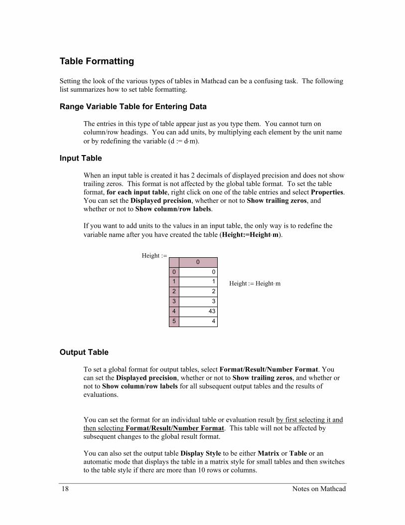
Table Formatting Setting the look of the various types of tables in Mathcad can be a confusing task. The following list summarizes how to set table formatting. Range Variable Table for Entering Data

The entries in this type of table appear just as you type them. You cannot turn on column/row headings. You can add units, by multiplying each element by the unit name or by redefining the variable (d := d⋅m).

Input Table

When an input table is created it has 2 decimals of displayed precision and does not show trailing zeros. This format is not affected by the global table format. To set the table format, for each input table, right click on one of the table entries and select Properties. You can set the Displayed precision, whether or not to Show trailing zeros, and whether or not to Show column/row labels. If you want to add units to the values in an input table, the only way is to redefine the variable name after you have created the table (Height:=Height⋅m).

Height0

01

2

3

4

5

01

2

3

43

4

:=

Height Height m⋅:=

Output Table

To set a global format for output tables, select Format/Result/Number Format. You can set the Displayed precision, whether or not to Show trailing zeros, and whether or not to Show column/row labels for all subsequent output tables and the results of evaluations. You can set the format for an individual table or evaluation result by first selecting it and then selecting Format/Result/Number Format. This table will not be affected by subsequent changes to the global result format. You can also set the output table Display Style to be either Matrix or Table or an automatic mode that displays the table in a matrix style for small tables and then switches to the table style if there are more than 10 rows or columns.

18 Notes on Mathcad

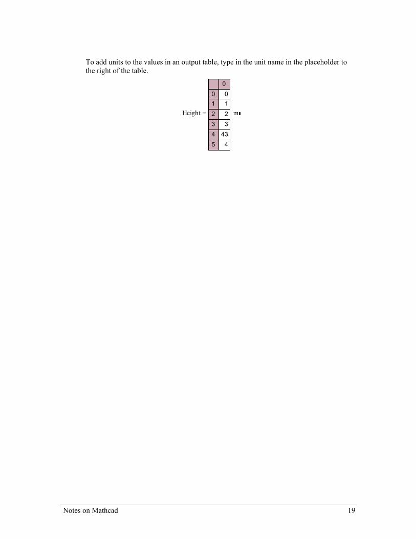
To add units to the values in an output table, type in the unit name in the placeholder to the right of the table.

Height

0

01

2

3

4

5

01

2

3

43

4

m=

Notes on Mathcad 19

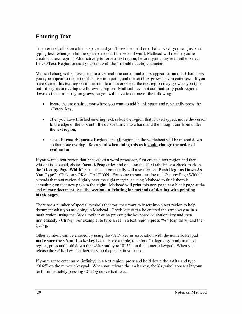
Entering Text To enter text, click on a blank space, and you’ll see the small crosshair. Next, you can just start typing text; when you hit the spacebar to start the second word, Mathcad will decide you’re creating a text region. Alternatively to force a text region, before typing any text, either select Insert/Text Region or start your text with the “ (double quote) character. Mathcad changes the crosshair into a vertical line cursor and a box appears around it. Characters you type appear to the left of this insertion point, and the text box grows as you enter text. If you have started this text region in the middle of a worksheet, the text region may grow as you type until it begins to overlap the following region. Mathcad does not automatically push regions down as the current region grows, so you will have to do one of the following:

• locate the crosshair cursor where you want to add blank space and repeatedly press the

<Enter> key,

• after you have finished entering text, select the region that is overlapped, move the cursor to the edge of the box until the cursor turns into a hand and then drag it our from under the text region,

• select Format/Separate Regions and all regions in the worksheet will be moved down so that none overlap. Be careful when doing this as it could change the order of evaluation.

If you want a text region that behaves as a word processor, first create a text region and then, while it is selected, chose Format/Properties and click on the Text tab. Enter a check mark in the “Occupy Page Width” box—this automatically will also turn on “Push Regions Down As You Type”. Click on <OK>. CAUTION: For some reason, turning on “Occupy Page Width” extends that text region slightly over the right margin, causing Mathcad to think there is something on that new page to the right. Mathcad will print this new page as a blank page at the end of your document. See the section on Printing for methods of dealing with printing blank pages. There are a number of special symbols that you may want to insert into a text region to help document what you are doing in Mathcad. Greek letters can be entered the same way as in a math region: using the Greek toolbar or by pressing the keyboard equivalent key and then immediately <Ctrl>g. For example, to type an Ω in a text region, press “W” (capital w) and then Çtrl>g. Other symbols can be entered by using the <Alt> key in association with the numeric keypad—make sure the <Num Lock> key is on. For example, to enter a ° (degree symbol) in a text region, press and hold down the <Alt> and type “0176” on the numeric keypad. When you release the <Alt> key, the degree symbol appears in your text. If you want to enter an ∞ (infinity) in a text region, press and hold down the <Alt> and type “0165” on the numeric keypad. When you release the <Alt> key, the ¥ symbol appears in your text. Immediately pressing <Ctrl>g converts it to ∞.

20 Notes on Mathcad

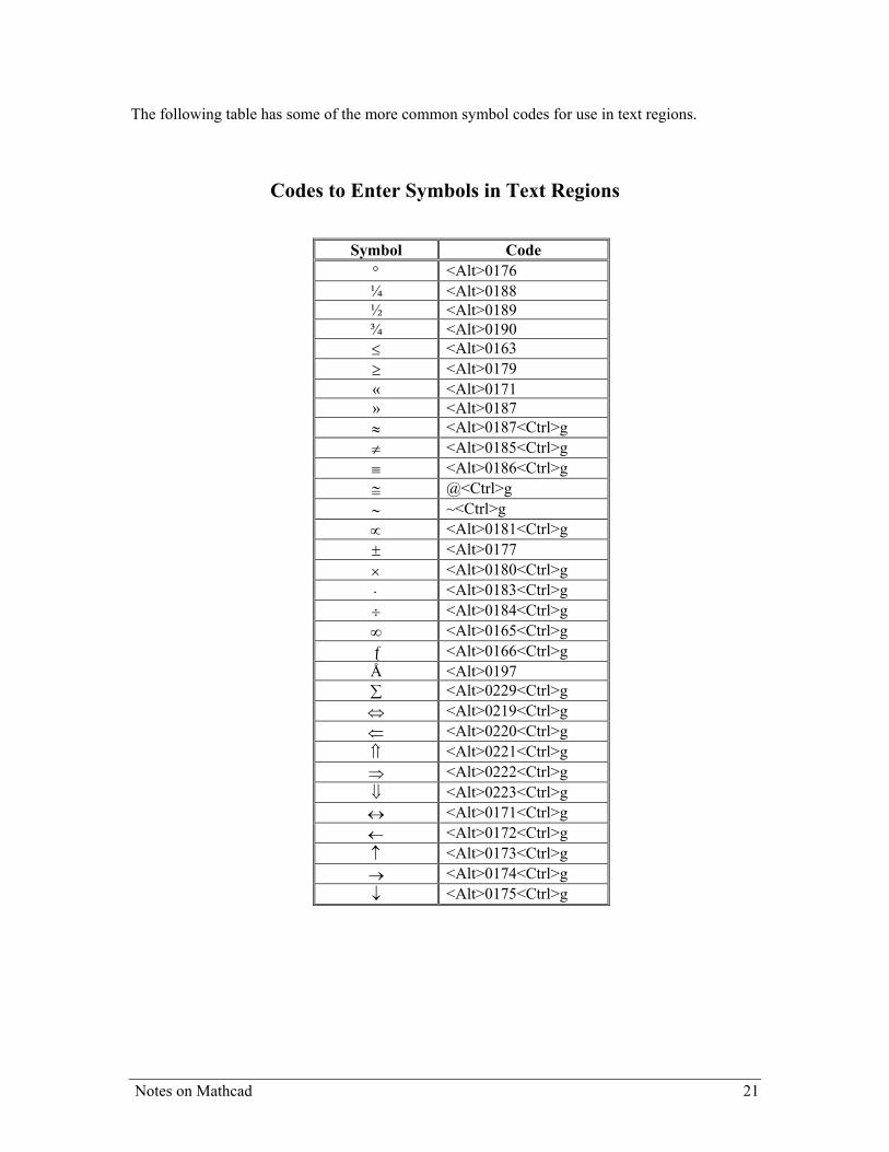
The following table has some of the more common symbol codes for use in text regions.

Codes to Enter Symbols in Text Regions

Symbol Code ° <Alt>0176 ¼ <Alt>0188 ½ <Alt>0189 ¾ <Alt>0190 ≤ <Alt>0163 ≥ <Alt>0179 « <Alt>0171 » <Alt>0187 ≈ <Alt>0187<Ctrl>g ≠ <Alt>0185<Ctrl>g ≡ <Alt>0186<Ctrl>g ≅ @<Ctrl>g ∼ ~<Ctrl>g ∝ <Alt>0181<Ctrl>g ± <Alt>0177 × <Alt>0180<Ctrl>g ⋅ <Alt>0183<Ctrl>g ÷ <Alt>0184<Ctrl>g ∞ <Alt>0165<Ctrl>g ƒ <Alt>0166<Ctrl>g Å <Alt>0197 ∑ <Alt>0229<Ctrl>g ⇔ <Alt>0219<Ctrl>g ⇐ <Alt>0220<Ctrl>g ⇑ <Alt>0221<Ctrl>g ⇒ <Alt>0222<Ctrl>g ⇓ <Alt>0223<Ctrl>g ↔ <Alt>0171<Ctrl>g ← <Alt>0172<Ctrl>g ↑ <Alt>0173<Ctrl>g → <Alt>0174<Ctrl>g ↓ <Alt>0175<Ctrl>g

Notes on Mathcad 21

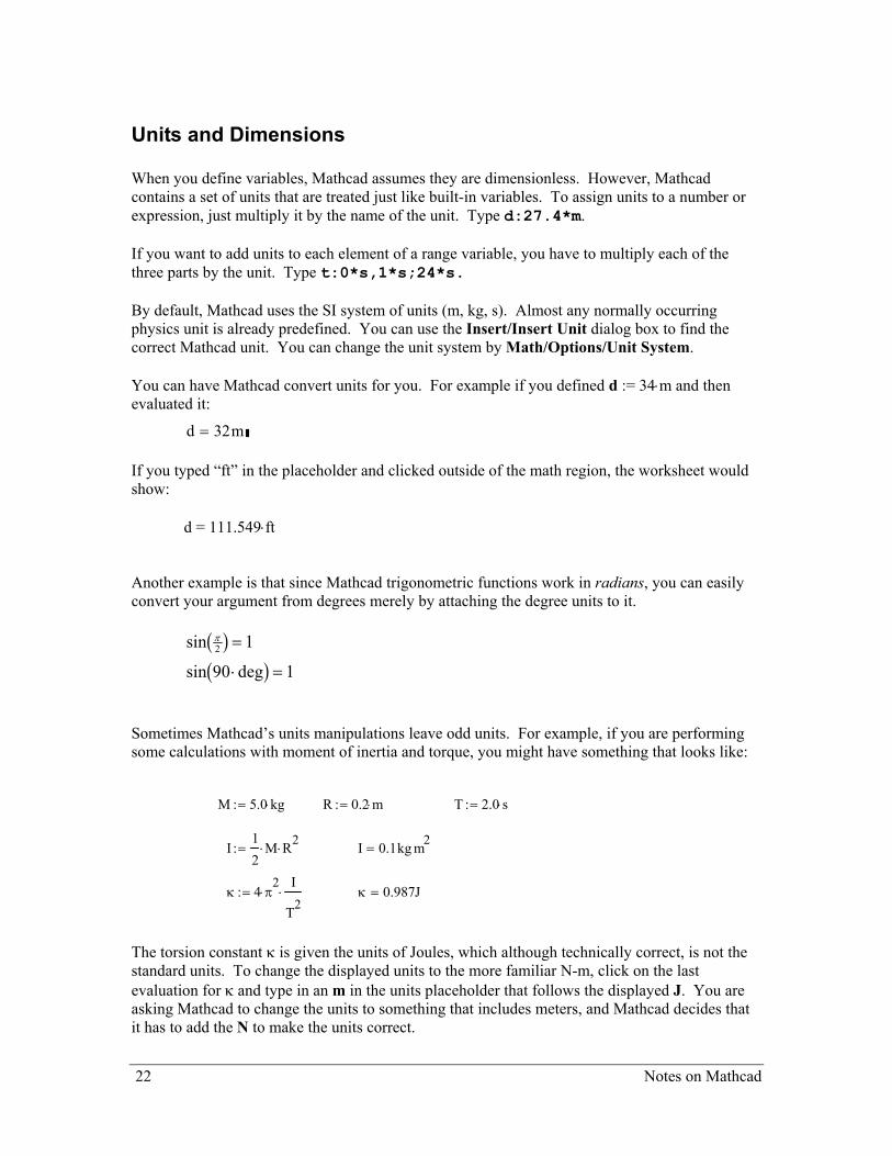
Units and Dimensions When you define variables, Mathcad assumes they are dimensionless. However, Mathcad contains a set of units that are treated just like built-in variables. To assign units to a number or expression, just multiply it by the name of the unit. Type d:27.4*m. If you want to add units to each element of a range variable, you have to multiply each of the three parts by the unit. Type t:0*s,1*s;24*s. By default, Mathcad uses the SI system of units (m, kg, s). Almost any normally occurring physics unit is already predefined. You can use the Insert/Insert Unit dialog box to find the correct Mathcad unit. You can change the unit system by Math/Options/Unit System. You can have Mathcad convert units for you. For example if you defined d := 34⋅m and then evaluated it:

d 32m= If you typed “ft” in the placeholder and clicked outside of the math region, the worksheet would show: d = 111.549⋅ft Another example is that since Mathcad trigonometric functions work in radians, you can easily convert your argument from degrees merely by attaching the degree units to it.

sin

sin deg

π2 1

90 1b gb g

=

⋅ =

Sometimes Mathcad’s units manipulations leave odd units. For example, if you are performing some calculations with moment of inertia and torque, you might have something that looks like:

M 5.0 kg⋅:= R 0.2 m⋅:= T 2.0 s⋅:=

I12

M⋅ R2⋅:= I 0.1kg m2

=

κ 4 π2

⋅I

T2⋅:= κ 0.987J=

The torsion constant κ is given the units of Joules, which although technically correct, is not the standard units. To change the displayed units to the more familiar N-m, click on the last evaluation for κ and type in an m in the units placeholder that follows the displayed J. You are asking Mathcad to change the units to something that includes meters, and Mathcad decides that it has to add the N to make the units correct.

22 Notes on Mathcad

Clicking on the evaluation looks like:

κ 0.987J= and then typing in the m at the placeholder and clicking outside the region yields:

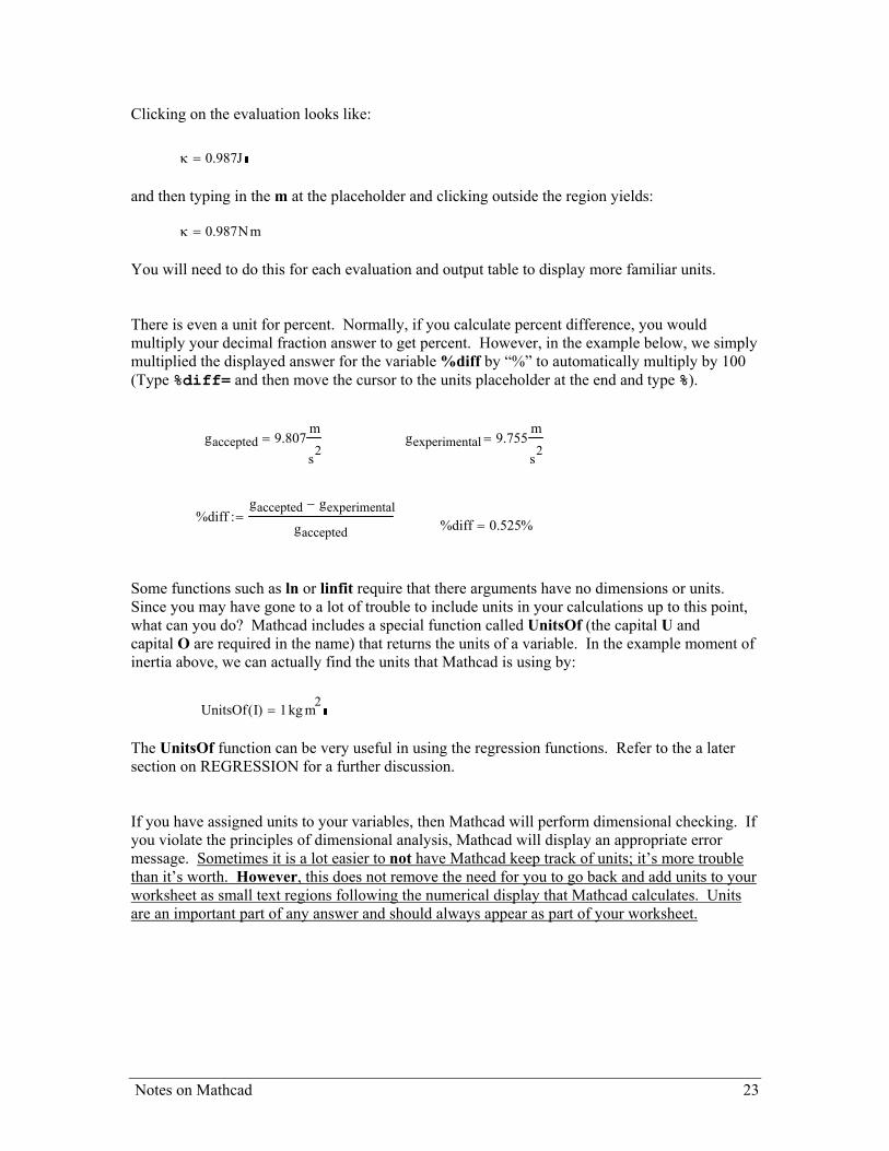
κ 0.987Nm= You will need to do this for each evaluation and output table to display more familiar units. There is even a unit for percent. Normally, if you calculate percent difference, you would multiply your decimal fraction answer to get percent. However, in the example below, we simply multiplied the displayed answer for the variable %diff by “%” to automatically multiply by 100 (Type %diff= and then move the cursor to the units placeholder at the end and type %).

gaccepted 9.807m

s2= gexperimental 9.755

m

s2=

%diffgaccepted gexperimental−

gaccepted:= %diff 0.525%=

Some functions such as ln or linfit require that there arguments have no dimensions or units. Since you may have gone to a lot of trouble to include units in your calculations up to this point, what can you do? Mathcad includes a special function called UnitsOf (the capital U and capital O are required in the name) that returns the units of a variable. In the example moment of inertia above, we can actually find the units that Mathcad is using by:

UnitsOf I( ) 1kg m2=

The UnitsOf function can be very useful in using the regression functions. Refer to the a later section on REGRESSION for a further discussion. If you have assigned units to your variables, then Mathcad will perform dimensional checking. If you violate the principles of dimensional analysis, Mathcad will display an appropriate error message. Sometimes it is a lot easier to not have Mathcad keep track of units; it’s more trouble than it’s worth. However, this does not remove the need for you to go back and add units to your worksheet as small text regions following the numerical display that Mathcad calculates. Units are an important part of any answer and should always appear as part of your worksheet.

Notes on Mathcad 23

Plotting To visually represent an expression or input data, Mathcad has a number of 2D and 3D plotting capabilities. Initially, the most important type for us is the 2D X-Y plot. You can start a plot by placing the crosshair where you want the plot, selecting Insert/Graph/X-Y Plot, selecting X-Y Plot from the Graph toolbar or by pressing the “@” key. Now fill in the X-axis and Y-axis placeholders with the names of the appropriate variables and click outside the plot region. To change scales, ticks, colors, etc., right click on the plot and select Format.

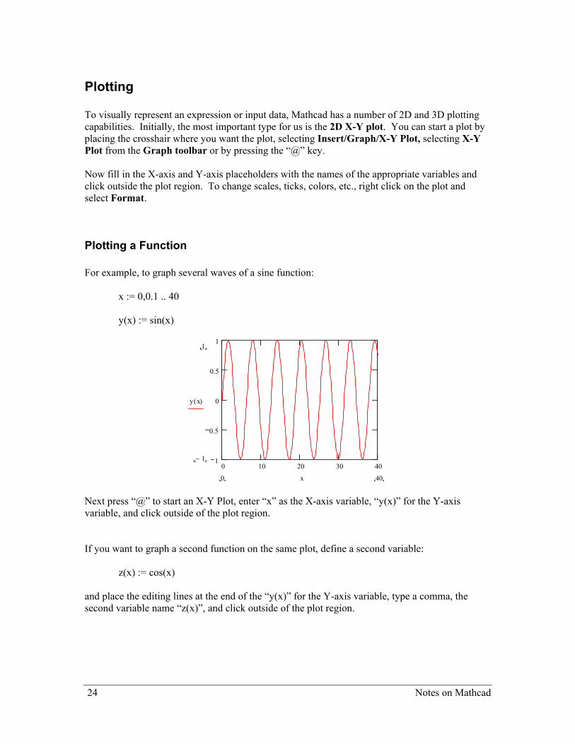
Plotting a Function For example, to graph several waves of a sine function: x := 0,0.1 .. 40 y(x) := sin(x)

0 10 20 30 41

0.5

0

0.5

11

1−

y x( )

400 x

0

Next press “@” to start an X-Y Plot, enter “x” as the X-axis variable, “y(x)” for the Y-axis variable, and click outside of the plot region. If you want to graph a second function on the same plot, define a second variable: z(x) := cos(x) and place the editing lines at the end of the “y(x)” for the Y-axis variable, type a comma, the second variable name “z(x)”, and click outside of the plot region.

24 Notes on Mathcad

0 10 20 30 41

0.5

0

0.5

11

1−

y x( )

z x( )

400 x

0

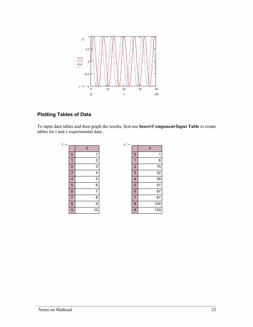
Plotting Tables of Data To input data tables and then graph the results, first use Insert/Component/Input Table to create tables for t and v experimental data.

t0

01

2

3

4

5

6

7

8

9

12

3

4

5

6

7

8

9

10

:= v0

01

2

3

4

5

6

7

8

9

16

15

22

39

51

67

81

104

133

:=

Notes on Mathcad 25

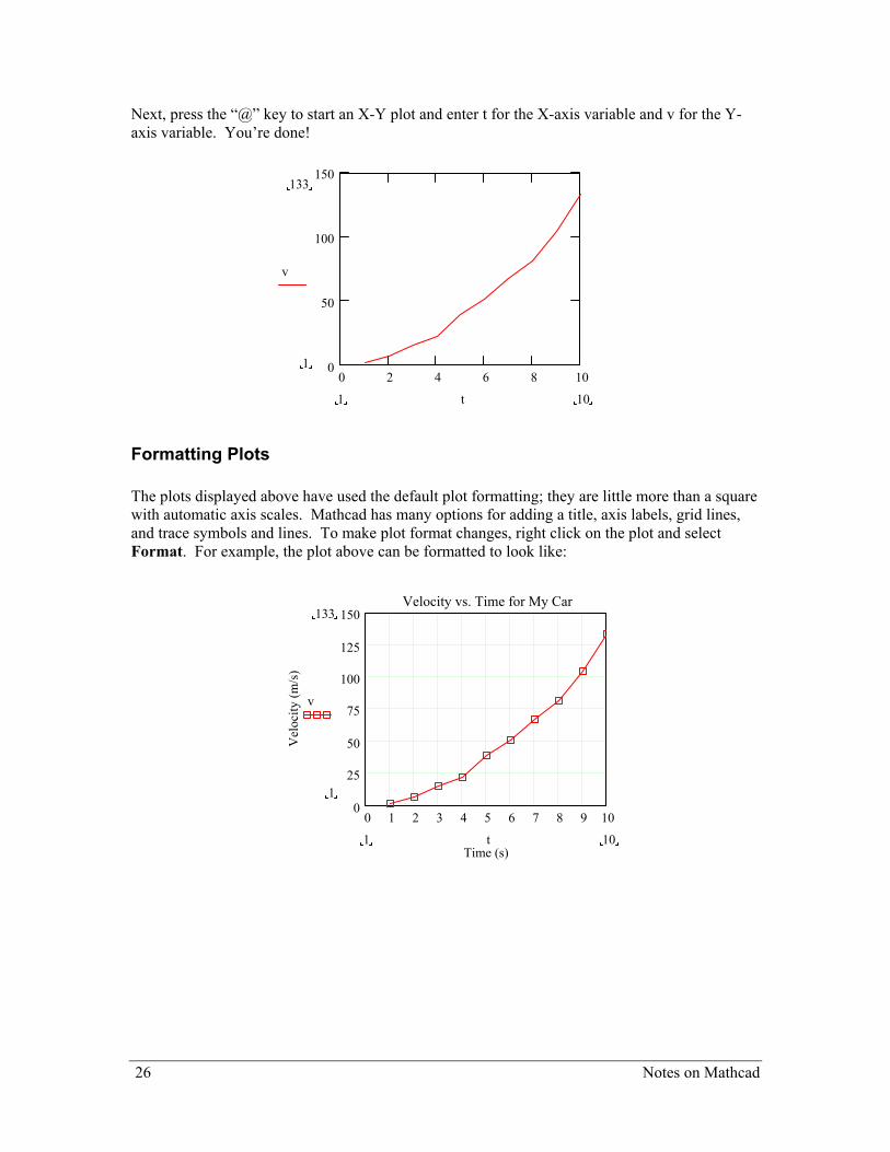
Next, press the “@” key to start an X-Y plot and enter t for the X-axis variable and v for the Y-axis variable. You’re done!

0 2 4 6 8 100

50

100

150133

1

v

101 t

Formatting Plots The plots displayed above have used the default plot formatting; they are little more than a square with automatic axis scales. Mathcad has many options for adding a title, axis labels, grid lines, and trace symbols and lines. To make plot format changes, right click on the plot and select Format. For example, the plot above can be formatted to look like:

0 1 2 3 4 5 6 7 8 9 100

25

50

75

100

125

150Velocity vs. Time for My Car

Time (s)

Vel

ocity

(m/s

)

133

1

v

101 t

26 Notes on Mathcad

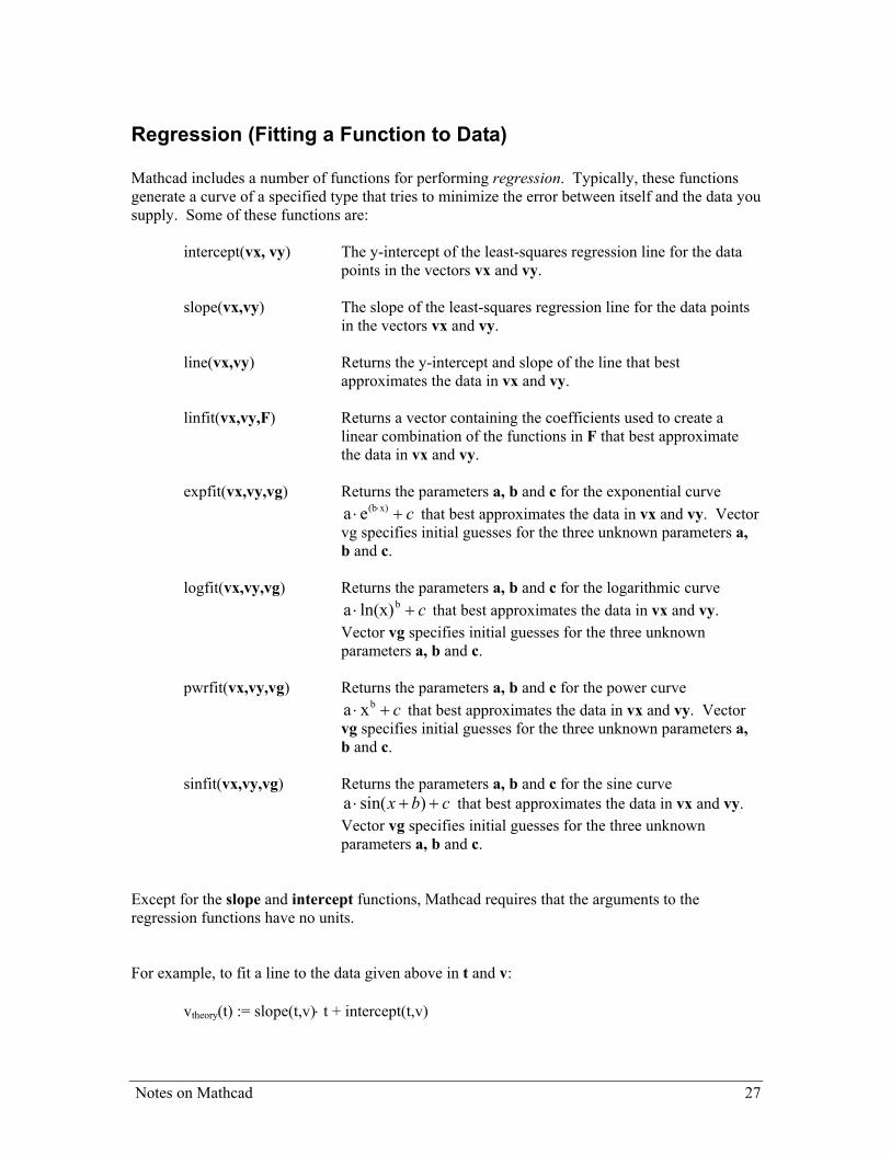
Regression (Fitting a Function to Data) Mathcad includes a number of functions for performing regression. Typically, these functions generate a curve of a specified type that tries to minimize the error between itself and the data you supply. Some of these functions are:

intercept(vx, vy) The y-intercept of the least-squares regression line for the data points in the vectors vx and vy.

slope(vx,vy) The slope of the least-squares regression line for the data points in the vectors vx and vy.

line(vx,vy) Returns the y-intercept and slope of the line that best approximates the data in vx and vy.

linfit(vx,vy,F) Returns a vector containing the coefficients used to create a linear combination of the functions in F that best approximate the data in vx and vy.

expfit(vx,vy,vg) Returns the parameters a, b and c for the exponential curve a e(b x)⋅ +⋅ c that best approximates the data in vx and vy. Vector vg specifies initial guesses for the three unknown parameters a, b and c.

logfit(vx,vy,vg) Returns the parameters a, b and c for the logarithmic curve that best approximates the data in vx and vy.

Vector vg specifies initial guesses for the three unknown parameters a, b and c.

a ln(x)b⋅ c+

pwrfit(vx,vy,vg) Returns the parameters a, b and c for the power curve a xb⋅ + c that best approximates the data in vx and vy. Vector vg specifies initial guesses for the three unknown parameters a, b and c.

sinfit(vx,vy,vg) Returns the parameters a, b and c for the sine curve a ⋅ + +sin( )x b c that best approximates the data in vx and vy. Vector vg specifies initial guesses for the three unknown parameters a, b and c.

Except for the slope and intercept functions, Mathcad requires that the arguments to the regression functions have no units. For example, to fit a line to the data given above in t and v: vtheory(t) := slope(t,v)⋅ t + intercept(t,v)

Notes on Mathcad 27

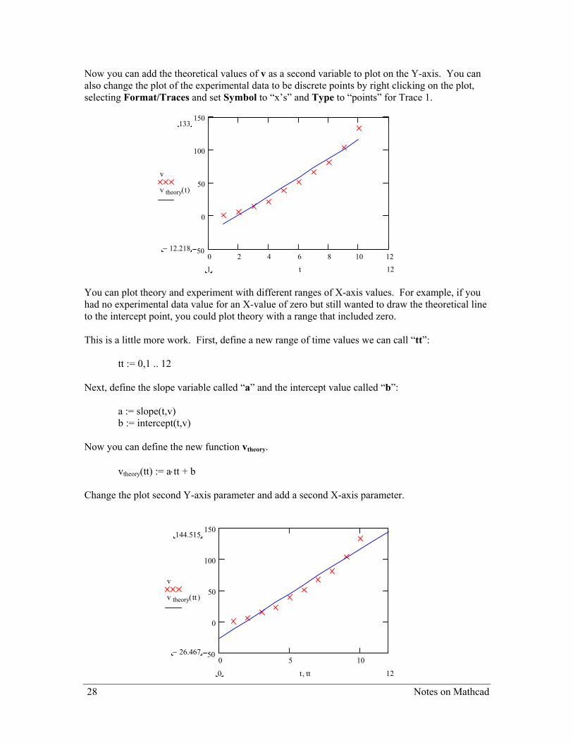
Now you can add the theoretical values of v as a second variable to plot on the Y-axis. You can also change the plot of the experimental data to be discrete points by right clicking on the plot, selecting Format/Traces and set Symbol to “x’s” and Type to “points” for Trace 1.

0 2 4 6 8 10 1250

0

50

100

150133

12.218−

v

v theory t( )

121 t You can plot theory and experiment with different ranges of X-axis values. For example, if you had no experimental data value for an X-value of zero but still wanted to draw the theoretical line to the intercept point, you could plot theory with a range that included zero. This is a little more work. First, define a new range of time values we can call “tt”: tt := 0,1 .. 12 Next, define the slope variable called “a” and the intercept value called “b”: a := slope(t,v) b := intercept(t,v) Now you can define the new function vtheory. vtheory(tt) := a⋅tt + b Change the plot second Y-axis parameter and add a second X-axis parameter.

0 5 1050

0

50

100

150144.515

26.467−

v

v theory tt( )

120 t tt,

28 Notes on Mathcad

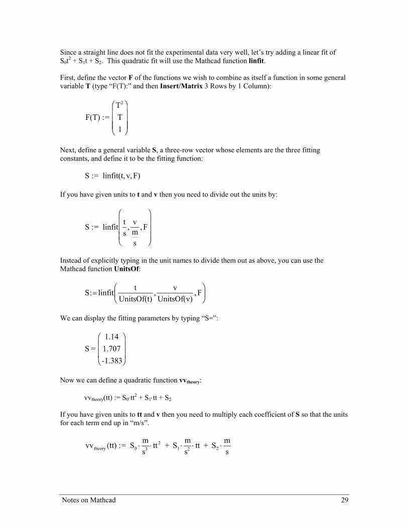
Since a straight line does not fit the experimental data very well, let’s try adding a linear fit of S0t2 + S1t + S2. This quadratic fit will use the Mathcad function linfit. First, define the vector F of the functions we wish to combine as itself a function in some general variable T (type “F(T):” and then Insert/Matrix 3 Rows by 1 Column):

F(T) :=TT1

2F

HGGG

I

KJJJ

Next, define a general variable S, a three-row vector whose elements are the three fitting constants, and define it to be the fitting function:

S := linfit(t, v,F) If you have given units to t and v then you need to divide out the units by:

S := linfit ts

vms

, F,

F

HGGG

I

KJJJ

Instead of explicitly typing in the unit names to divide them out as above, you can use the Mathcad function UnitsOf:

S: linfit tUnitsOf(t)

vUnitsOf(v)

F=FHG

IKJ, ,

We can display the fitting parameters by typing “S=”:

S =1.141.707-1.383

F

HGGI

KJJ

Now we can define a quadratic function vvtheory: vvtheory(tt) := S0⋅tt2 + S1⋅tt + S2 If you have given units to tt and v then you need to multiply each coefficient of S so that the units for each term end up in “m/s”.

vv (tt) := S ms

tt + S ms

tt + S mstheory 0 3

21 2 2⋅ ⋅ ⋅ ⋅ ⋅

Notes on Mathcad 29

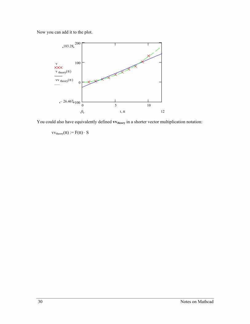
Now you can add it to the plot.

0 5 10100

0

100

200183.28

26.467−

v

v theory tt( )

vv theory tt( )

120 t tt, You could also have equivalently defined vvtheory in a shorter vector multiplication notation: vvtheory(tt) := F(tt) ⋅ S

30 Notes on Mathcad

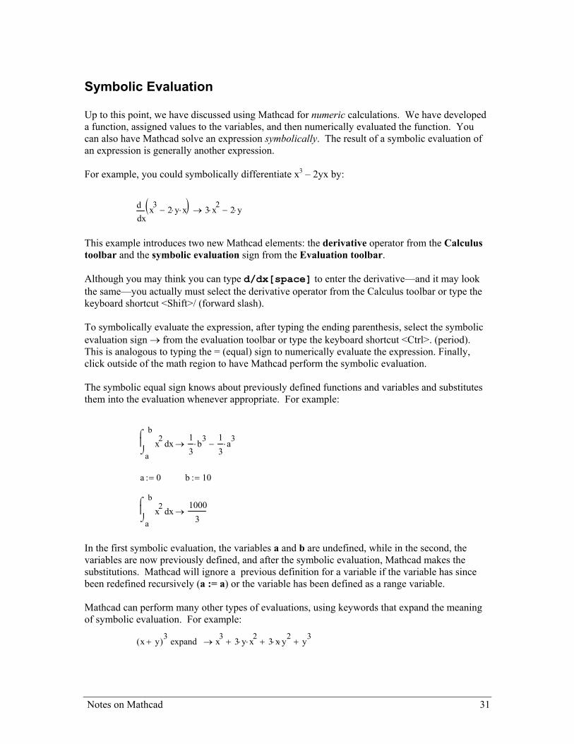
Symbolic Evaluation Up to this point, we have discussed using Mathcad for numeric calculations. We have developed a function, assigned values to the variables, and then numerically evaluated the function. You can also have Mathcad solve an expression symbolically. The result of a symbolic evaluation of an expression is generally another expression. For example, you could symbolically differentiate x3 – 2yx by:

xx3 2 y⋅ x⋅−( )d

d3 x2⋅ 2 y⋅−→

This example introduces two new Mathcad elements: the derivative operator from the Calculus toolbar and the symbolic evaluation sign from the Evaluation toolbar. Although you may think you can type d/dx[space] to enter the derivative—and it may look the same—you actually must select the derivative operator from the Calculus toolbar or type the keyboard shortcut <Shift>/ (forward slash). To symbolically evaluate the expression, after typing the ending parenthesis, select the symbolic evaluation sign → from the evaluation toolbar or type the keyboard shortcut <Ctrl>. (period). This is analogous to typing the = (equal) sign to numerically evaluate the expression. Finally, click outside of the math region to have Mathcad perform the symbolic evaluation. The symbolic equal sign knows about previously defined functions and variables and substitutes them into the evaluation whenever appropriate. For example:

a

b

xx2⌠⌡

d13

b3⋅

13

a3⋅−→

a 0:= b 10:=

a

b

xx2⌠⌡

d1000

3→

In the first symbolic evaluation, the variables a and b are undefined, while in the second, the variables are now previously defined, and after the symbolic evaluation, Mathcad makes the substitutions. Mathcad will ignore a previous definition for a variable if the variable has since been redefined recursively (a := a) or the variable has been defined as a range variable. Mathcad can perform many other types of evaluations, using keywords that expand the meaning of symbolic evaluation. For example:

x y+( )3 expand x3 3 y⋅ x2⋅+ 3 x⋅ y2

⋅+ y3+→

Notes on Mathcad 31

uses the expand keyword evaluation from the Symbolic toolbar. Alternatively, you could select the Keyword Evaluation symbol →or type <Ctrl><Shift> . (period) and type the keword in the placeholder. The following list contains just a few of the types of symbolic evaluations. A full list with explanations can be found in the on-line official Mathcad User’s Guide.

simplify Simplifies an expression performing arithmetic, canceling common factors, and using basic trigonometric and inverse function identities.

expand Expands all powers and products of sums in an expression.

factor Factors an expression into a product.

solve, var Solves an equation for the variable var.

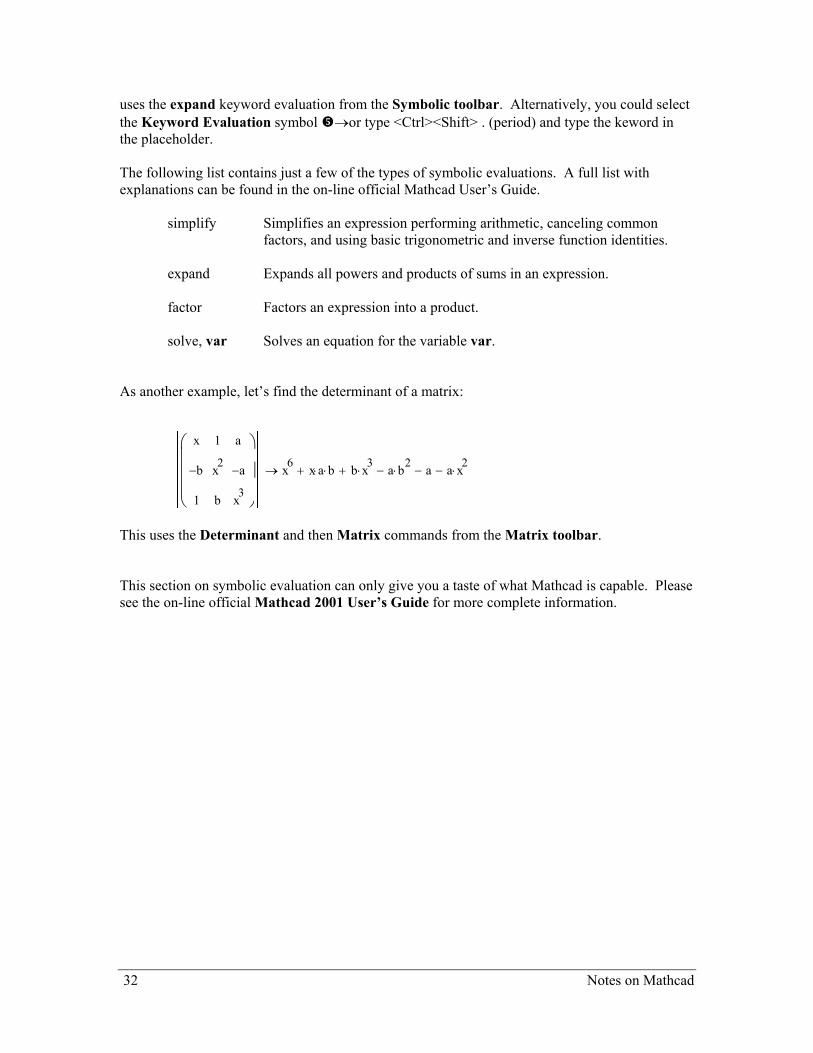
As another example, let’s find the determinant of a matrix:

x

b−

1

1

x2

b

a

a−

x3

x6 x a⋅ b⋅+ b x3⋅ a b2

⋅− a− a x2⋅−+→

This uses the Determinant and then Matrix commands from the Matrix toolbar. This section on symbolic evaluation can only give you a taste of what Mathcad is capable. Please see the on-line official Mathcad 2001 User’s Guide for more complete information.

32 Notes on Mathcad

Notes on Mathcad 33

Printing Scroll through the entire document to make sure it looks good, with no regions overlapping page breaks and no regions extending past the right margin. Make a note of the last page number N. After saving your Mathcad worksheet for a final time, go to the Print dialog box by selecting File/Print. Note where the Print dialog box says “Print range”. If the M in “All M pages” is the value you just wrote down for N, click on <OK>. If M is larger than the length of your worksheet, then there are some regions that extend beyond the right margin. The easiest solution is to change the print range to Pages from 1 to N to make sure you print only useful pages without extra blank pages at the end. Now click on <OK>.