A Short Way of Solving Advanced Problems in ... · A Short Way of Solving Advanced Problems in Electromagnetic Fields and Other Linear Systems* V. H ... tering and antenna problems,

1963 IEEE TRANSACTIOKS O N ANTENNAS AND PROPAGATIOhT 73

A Short Way of Solving Advanced Problems in Electromagnetic Fields and Other Linear Systems*

V. H. RUhISEYt, FELLOW, IRE

Summary-A linear system is characterized in the abstract by a source vector a, a response vector a and a system matrix (il, connected by =&. Speciiic interpretations for a, a and CR are given for electromagnetic fields, the scalar product a4R.b being the reaction. The advantages of this method are illustrated by application to vari- ous problems. Mode expansions are defined by the eigenvector equation am = Cmm, C, being the eigenvalue and m the modesource. This means the mode is generated by a combination of electric and magnetic sources which, apart from the constant multiplier C,, ‘are everywhere equal to the electric and magnetic fields, respectively. Such mode expansions are applied to typical waveguide problems. Waveguide theory is set up in terms of unit voltage and unit current mode sources, v and i, where v.v= 1 =i.i. Then the definitions of waveguide current and voltage coincide with those for circuit theory, e.g., the mode current at cross section P is the reaction on a unit voltage source placed at P. The method also greatly simplifies scattering and antenna problems, such as the pattern of a monopole antenna which is immersed in a layer of gyrotropic plasma.

A I. INTRODUCTION

FEW YEARS AGO during a Congressional hearing, the Voice of America mas criticized for putting some of its transmitters in Washington,

D. C., instead of nearer to Russia. To answer this criti- cism a receiver was brought into the hearing room and tuned to Radio iLIoscow, which came in loud and clear. This little story illustrates one of the aims of the present paper, namely, the power of the reciprocity theorem to answer difficult questions with devastating simplicity. Sow although the reciprocity theorem is well known, the classical theory of fields makes it rather difficult to apply to problems involving electromagnetic waves. Another aim is then to set up such problems in a radically simpler may, a way which makes the application of the reciprocity theorem practically automatic. The type of formulation we shall use is not new, however, having long been used in quantum theory and more recently in system theory. Indeed, it is the standard abstract theory of linear systems adapted to radio waves, but such an adaptation can be set up in many different ways, and at the outset it is far from clear which form is best. This brings us to the main point, which is the application of the abstract method to typical problems. In order to illustrate the power of the method many of these will be familiar problems whose solutions are well known, but the method will also be used to solve some new problems.

To introduce the approach let us consider the familiar representation of an electrostatic system of conduc-

* Received June 25, 1962. t UniversitJ. of California, Berkeley, Calif.

tors having charges Ql, Q z , Q 3 , and potentials p1, pz, 9 3 , - . - . Then in view of the linearity of the system, we have

Qi = CijpiJ (1) j

or inversely,

pi = aijQj. (2) i

The system is thus represented in terms of a vector a whose components are Q1, Q2, Q3, . . , a vector a whose components are pl, yz, y3, . . . , and a matrix defined by

a = (ila. ( 3 )

The extension of this to a continuous distribution of charge is fairly clear. The vector a now represents the charge density p,(x, y, z ) , the components of a being the values of pa a t different points ( x , y, z) ; in the same way a now represents the potential distribution p,(x, y, z) and (il is defined in terms of a and a by (3). Thus a and a now have an infinite continuous set of components, and therefore (il does also. The scalar product of two such vectors is likewise the obvious extension of the scalar product for the discrete case. Specifically, if b represents another charge density P b ( X , y, z) and @ the corresponding potential distribution 96, the scalar products are defined by

a. b = p,pbdrdydz, integrated over all space (4) S S (5)

S (6)

0 = p,pbdxdydz

b*a = pbp,,dXdydz.

Speaking now in general terms, the basis of the method is to represent the state of a system by a source vector a, a response vector a, and a system matrix defined by ( 3 ) . (Vectors like a , for which the scalar product is defined by an integral like (4), ( 9 , or (6), are discussed in many places-see for example Dirac [l], Morse and Feshbach [2], Friedman [SI, and Bresler and Marcu- vitz [4]).

a’’ in more meaningful, just as “vector a” is more meaningful than 1 Conventionally, one speaks of the “operator R” but “Matrix

“operand a.”

Authorized licensed use limited to: Princeton University. Downloaded on December 3, 2009 at 17:06 from IEEE Xplore. Restrictions apply.

. -2 , .- -~

-. 74 ~.

IEEE TRANSACTIONS ON ANTENhTAS AND PROPAGATION January

To apply this method, we think of a typical practical problem in the following way. Suppose that we wish to find the voltage received by a certain antenna from some distant source represented by a. Then we introduce what may be called a test source, represented by b, which is chosen so that i t “tests” the voltage pro- duced by source a; in this case b turns out to be a unit current generator connected to the terminals where the voltage from a is to be measured. Then the scalar product b . @a is the voltage to be found. Now we have pur- posely left out the details of how we choose the proper test source and how i t comes about that b - @a is the voltage received from a, in order to concentrate atten- tion on the idea of introducing a test source. To give a simple example in which the details can easily be worked out from what has already been said about electrostatics, if b represents a unit charge at point xl, yl, zl, by (61,

b. @a = pu(xl, yl, zl). ( 7)

Thus b tests the potential. Likewise, the reader will easily discover from (1) . . . (6) that to test the electric field the proper test source is a unit dipole. Explicitly, if b is a dipole of unit moment parallel to the x axis at (x11 Y1, Z l ) ,

It may also be helpful to look at (7) from the abstract vector point of view. Since pu(xl, y1, 21) is by definition the “component” of @a in a particular “direction,” the way to pick it out is to take the scalar product of @a with the unit vector in this direction. Thus the unit test source a t a particular position is represented by a “unit vector” b in a particular “direction.”

Now from ( 6 ) , the well known reciprocity theorem for electrostatics (Green’s reciprocation theorem) gives

b. @a = a- @ - b, for all a and b. (9)

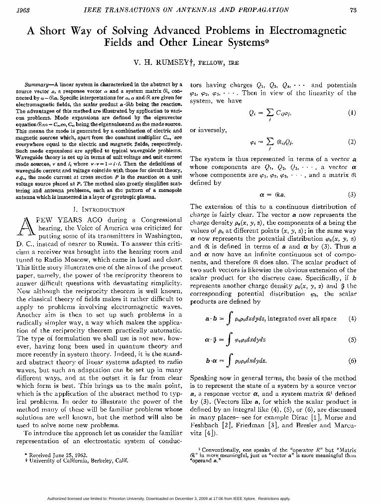
To illustrate the importance of (9), let us consider the following problem, shown in Fig. 1. Suppose that a charge Qa is placed at Y = Y O between two concentric metal spheres, the outer one Y = rl being grounded. We wish to find the potential of the inner one Y = ~ 2 . There- fore, we put a unit test charge b on the inner sphere. Then if a represents Qu

pU(r2 ) = b- @a = a. @b = Qapb(ro). ( 10)

But pb(r0) is easy to find:

1 1 1

4irE Y 1 ro %(YO) = ~ (- - --),

and hence pa(r2) is immediately obtained. Alternatively, had we not put in the test source, we could have set about finding the potential distribution due to Q. b y means of a spherical harmonic expansion. We see that

Fig. 1--X charge Qa between two spheres.

even in this simple example there is a striking difference between the two methods, the former being much the shorter. Sow, to be sure, this is just a rudimentary application of the reciprocity theorem, but the point is that (9) can lead to drastic simplification, and in the case of more advanced problems these simplifications can be fairly described as astounding.

The elements of (R are related to the classical Green’s function. For example (2) and (3) show that aij is the potential at the ith conductor due to unit charge on the j t h conductor, and so for a continuous system an ele- ment @(PQ) can be interpreted as the potential at P due to unit charge at Q, which is the Green’s function. However, the identification of @ with the Green’s function is not so clear for the more general cases considered in the next section. Our method differs from the Green’s function method in that we always work in terms of two sources, a and b, and their fields. This difference is apparent even for the simple problem of the previous paragraph. Instead of working with a function, our fundamental quantity is an integral, namely a- ab. We are, so to speak, dealing with an integral transform of the field. What a difference this makes will be seen when we discuss Huygens’ principle, or, for a much more ex- tensive illustration, see Rumsey [ 6 ] . For example, instead of trying to find the field of an antenna (which implies finding an infinite set of numbers), we solve for the voltage received from this antenna in a specific measurement (which is a single number). Thus our method is more a theory of practical measurements than a theory of fields. In terms of the abstract vectors, instead of trying to find all the components of @a, we solve for the single component b. @a.

The mathematical advantages of dealing with the integral b - @a are, of course, highly significant when- ever we need to deal with singular fields and singular source functions. For example, the field pa and the source function p a of a point charge are singular, so much so that p a cannot properly be called a function, yet these serious difficulties simply do not arise if we deal with b o @a (for any b different from a). In this sense, our method can be regarded as an application of the


1963 Rzcmsey : Solring Bdtlanced Problem in Electromagnetic Fields

Schwartz theory of distributions; b - @a can be under- stood as the distribution corresponding to the function y, (or, in an extended sense, the function pa) with Pb taking the role of the testing function.

11. DEFINITIONS OF REACTION

Since b - @a is the key factor in the theory and its physical interpretation, it is convenient to give it a name-the reaction of source b on source a. (In previous publications [5]-[10] i t has been denoted by (ab) but the present notation appears to be preferable.) We see that the definition of reaction depends on some form of reciprocity theorem, and therefore we base i t on that form of reciprocity theorem which applies to the larg- est class of physical systems. The class of systems to be considered may have any distribution of permeability p, permittivity E , and conductivity u, and may be anisotropic and heterogeneous, but must satisfy the radiation condition a t infinity; or, if the system is closed, the mall of t he enc losure must correspond to a passive impedance. In other words, we are dealing with the “retarded” type of solution of Maxwell’s equations. This implies that , given the source function, the response function (E or H) is unique with the possible exception of a resonant cavity field. We therefore add the restriction that the frequency does not coincide with any resonance of the system, thus ensuring uniqueness under all circumstances.

The definitions to follow are given in two forms: one is a volume integral over the source a and the other is an integral over a closed surface S which does not con- tain the source functions directly. The two forms are equivalent, provided we can find a surface S, such that source a is entirely inside S and source b is entirely outside S. (For example, S does not exist if a =b.) The symbol N represents a unit vector normal to S pointing outwards. The subscript a on y,, E,, etc., means the potential, electric vector, etc.,. due to source a.

i) For electrostatics, P being the dipole density, as in

V.(EE f P) = p , (12)

a . (Flb = (papb - P,.Eb)d.Td)”dZ S (13) =x~(miE. - pn%) (1.1)

ii) For magnetostatics, J and M, being the densities of current and magnetization, as in

J = V X H , (15)

B = p ( H + M ) = V X A , (16)

a . ab = ( Ja.Ab f M,.Bp,)dxdydz S (17)

(A X Hb - Ab X Ha) .NdS. (18)

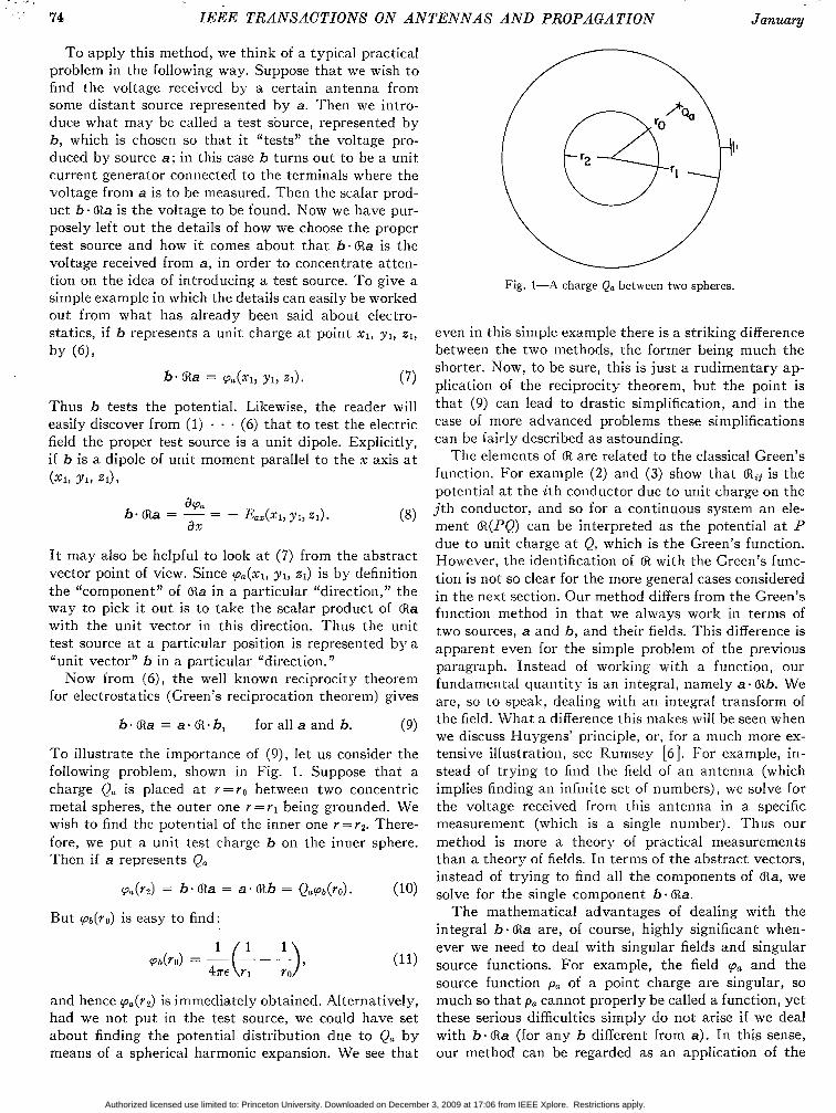
3 Fig. 2-A passive network.

75

I I

Fig. 3-The network excited by source a.

iii) For radio waves with the expjwt time convention, J and K representing the densities of electric and magnetic dipoles, as in

J + (u +jue)E = V X H, (19)

K + j ~ p H = - B X E, (20)

a . ab == (J,.Eb - &.Hb)d.Td)dZ S (20) =x(& x H b - E b X Ha) .SdS. (22)

iv) For ac circuits, position in the circuit is denoted bs; the subscript n = 1, 2, 3, . . . as in Figs. 2 and 3. Small letters zl,, and i,, denote the voltage and current sources which comprise source a and large letters Vu, and I,,, denote the response due to source a. Thus I b n is the current due to source b through the voltage source van and source a consists of the combination of zUl, vU2, . . . and ial, i,?, . . . . Then

a . ab = T a n I b n - ianJ’’bn, (23) n

the sign convention being such that the voltage Van across any current source ia, would be positive if i,, were connected to a resistor and the current I,, through any voltage source van would be positive if van were connected to a resistor, as in Fig. 3.

111. DEFINITIONS OF SOURCE VECTORS AKD RESPOXSE VECTORS

The interpretation of a as an abstract vector in 1) has been extended beyond what was said in Section I by the addition of the dipole density P,. The components of a now comprise not only all the values of


76 IEEE TRANSACTIONS ON ANTENNAS AND PROPAGATION January

pa(%, y , z) a t different points x , y , z, but all the values of Paz(x, y , z) , P,(x, y , z) and Pa,(%, y , z). Likewise, the components of the abstract vector @ = (Rb in 1) comprise all the values of -(x, y , z ) , -Eh(x, y , z ) , -Eh(x , y , z) and -&(X, y , z) . The interpretation of the components of a and @ in 2) follows the same lines. Cases 3) and 4) can be considered together because 4) is a special case of 3). Nom7 in 4) i t may look as though the components of a could be taken as

Val, Va? * ' ' j z a l ) J'Za2 * , .. .. (24)

and then the components of a= (Ra would have to be

101, I a 2 * * * jVa17 j V a 2 * . (25)

in order to fit (23). This would fix the definition of the complex conjugates & and 3 and hence the definition of & also. Unfortunately, this definition of $ turns out to be inconsistent with the physical interpretation. For example, it is impossible t o find values of p, E and u (even allowing negative values of p and e) such that source 2 in system $ gives a. I t turns out that in order to make & meaningful, we must define 3 by the relations

22 = ia and 0:: = va

which are not consistent with (24). We therefore take

X X (26)

a = @

CY = (Ial7IaZ, * * -Val7 -Vase, * - ). (28)

. . b a l , v,?, * * - z,l, za2, - ), and (27)

Then,

a 4 = I D a n ] ? + I ian 12 (29)

a.2 = I I a n / ? + I v a n ] ? (3 0)

n

n

but X a. @a = G a n ~ a n - zanvUn). (3 1)

x n

When there are no current sources, it will be seen from (27) and (28) that (R is the conventional impedance matrix of the network, defined with respect to the terminals of the voltage sources.

Similarly in 3) we take

a = a, + a, + a,, (32)

a = a z + a, + a=> (33)

a, = [-EUz(rd7 -Kuz(r2), . . . ~ , , ( r ) , ~ ~ ~ ( r a ) - . * I , (34)

az = [auz(rl), HRI(r?) ) . + - -E,(rJ, Eaz(r2) * * I , (35)

any abstract vector with subscript x being orthogonal to any abstract vector with subscript y or z. With these definitions, & represents the conjugate system-that in which all impedances are replaced by their conjugates.

IV. PROPERTIES OF THE SYSTEM MATRIX

The condition

a - (Rb = b - ma, for all a and b, (9)

which me first met in Section I as a statement of Green's reciprocation theorem, says the matrix @ is symmetric. If 5 is defined by - a.. = @..

23 3 I for all i a n d j (36)

[see (3)], ;.e., 6i denotes the transpose of a, (9) says

(R = a. The physical significance of g is this. In an isotropic medium, (R and are the same. In an anisotropic medium p, e, and u are represented by matrices,(second- order tensors). If p , E and 5 represent the tensors p, e, and u transposed, represents the system characterized by p , E, and 5 in place of p, E, and u ; in other words, the transposed system. Now (R is in fact symmetric for i) and ii) and, with the exception of gyrotropic media, for iii) and iv) also.

- (3 7)

Even when @ is not symmetric, the relation

a - @ b = b-&a, (3 8)

which is merely the definition of % in the abstract theory, represents an important result which is very far from obvious. I t says, if 8, and a, represent the field of source a in the transposed system,

(Ja.Eb - &.Hg)dxdydz

= ( J b + E , - Kb.I%)drdydz (39)

for all sources a and b in class iii). Likewise the relation

X x x (:- ab) = a . (40)

which is merely an application of the elementary ru1.e for taking the complex conjugate, summarizes another important result in the physical interpretation. The point is not that a result like (39) can be proved b y using (38). On the contrary, results like (39) must first be discovered t o indicate the appropriate definitions for a, a and (R. The point is that once the abstract for- malism has been properly set up, it expresses very simply, indeed automatically, important results which otherwise are hard to grasp and hard to use.

For gyrotropic lossless media fi =$ and Z = v , but from this well-kncwn result we cannot jump to the conclusion that %= @. For a lossless, nonradiating system we find that

b-&a = + b.&a (111)

if a and b are unlike sources, namely one is electric and the other magnetic. rf a and b are sources of the same type,

6 . a a = - bX~ila. (42)


1963 Rumsey : Solving Ad,mnced P r o b l m i n Electromagmtic Fields 77

Fields in conjugate systems with u=O are closely related to the advanced solutions of Maxwell's equations. To explain this, let us use the bar over E or H to denote the advanced type of solution so that on the sphere a t infinity

but

i being the unit radial vector. Let a denote the advanced system matrix as @ denotes the retarded system matrix. Thus,

- (Y = @a (42a)

denotes the advanced solution that goes with source a ; a represents E,H, as a represents E,H,. Now for u=O it is not difficult t o show, even for gyrotropic media, that

- _ -

integrated over all space. Hence for like sources (K,=O=Kb or J a = O = J,)

x x - x a . @ b = - k-Cta = - a . @ b (424

and for unlike sources

x x a.ab = b.@a = a-ab". (424

From (42c) we see that for radiating gyrotropic systems with no ohmic loss

X - @ = - a (424

for test sources of the same kind as the source being tested, and

& = 6, otherwise. (420

For nonradiating systems these results, when combined with (41) and (42), reduce to the statement

@ = a, which merely says there is no distinction between the advanced and retarded solutions for a closed lossless cavity.

T o finish off this discussion of the properties of the system matrix 6 i , i t may be as well to point out another false conclusion which may creep in unquestioned, namely, that (R = 6 i l - a2 does not represent the system characterized by p = p 1 -p2, E = e l - € 2 , and u =u1 -uz.

V. HUPGENS' PRINCIPLE The purpose of this Section is to illustrate how the

abstract vector method works. We will not at tempt an

exhaustive discussion because a fairly complete account has already been published [6], nor will we derive any new results because this aspect is also covered in the same publication.

I t is clear from the definitions of Section IV tha t if u and v are two sources such that

t - (Ru = t - av, for all t , then (43)

u = v, (44)

or, in the physical interpretation, the effects of sources u and v in system (R are identical. Now, with reference to (14), let c represent the surface charge density eE, .N (on 5') and d the surface dipole density epaN. Then (13) and (14) say

b-@a = a . @ b = (c + d ) . & b = b.(R(c + d) (45)

for all b outside S. Hence the combination of the surface charges &,.N and surface dipoles E ~ , N is equivalent to a for all points of observation outside S. Note the generality of this proof: it applies to any heterogeneous anisotropic medium. For example, when E is a tensor, the dipoles in d are not aligned normal to S.

Now i t is not difficult to show that (14) is valid i' the environment for source b is the same as that fol source a outside SI but not necessarily inside S. Thus

b * & = b * @ l ( c + d ) (46)

where system (Rl=system (R outside S but 6i1 is arbitrary inside S. Let us then choose @I= 6: where d: represents the system with a grounded conductor inside S (see Figs. 4 and 5 ) . Then if t is any test source

f - C c = c . G t = pcptdS (from the definition of c) A = 0, because pt = 0 on S (from the definition of 2).

:. c c = 0 (45)

:. b . (Ra= b .Cd , for all b. (48)

Hence, outside S, d in 6: is equivalent to a in a; in other words, the dipole density E ~ , . N on the outside of a grounded conductor coinciding with S gives the same field as the original source a. Alternatively, i f R1= % where system m has E = 0 inside SI

5nd = 0, and (49)

b-6ia = b.%c. (50)

Therefore, c in 5n is equivalent to a in a. Evidently, an analogous set of equivalence theorems

follows from (18) and (22). From (18) we see that we can take c as the surface currents NXH, and d as the surface dipoles p-lN XA,; likewise, from (22) we can take c as the surface electric dipoles N XH, and d as the surface magnetic dipoles E,XN. For (18) we take p = O (inside S) for 6: and p = co for YE; for (22) we take p = m

for 6: and E = for m. Then again a in (R is equivalent to c+d in (R1 or d in 6: or c in m.


78 IEEE TRAATSACTIOATS O N ANTENNAS AhTD PROPAGATION January

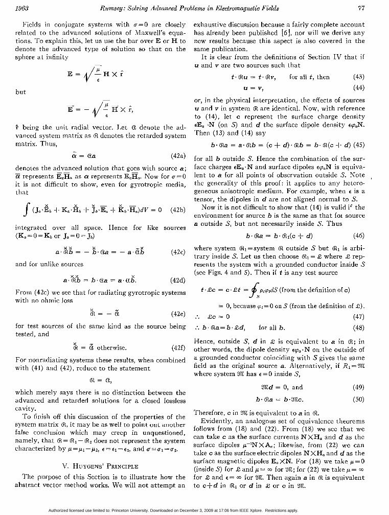
c+d T-- x x x x x x

Fig. 4-Sources a b c and d in system @.

c+d

Fig. 5-Sources a b c and d in system 2. 1

Although this discussion has touched only a small part of the subject, in view of what is already published, let us now turn to a different kind of application.

V I . M O D E EXPANSIONS The connection between the modes of a system and

the eigenfunctions of a certain linear operator is a familiar feature in textbooks on theoretical ph>-sics. How- ever, a systematic application to Maxwell’s equations does not seem to have been tried, yet mode expansions for Maxwell’s equations have in fact been the cause of considerable difficulty. We will first introduce the idea of a mode source by means of a simple example from electrostatics. This method will then be applied to a microwave cavity, and we will obtain an orthogonal set which contains a t least twice as many modes as the conventional expansions.

An eigenvector of the matrix @ is defined by

am = C m m (31)

where C,, the eigenvalue, is a scalar. For the sake of simplicity, let us apply (51) to an electrostatic system, in which the only kind of source is charge. Then (51) says

(Orn(Z, Y, 2) = Cm~m(x, Y) z ) ) (52)

or, for a uniform medium,

Pm (Om VZYm = - - = - - , (53)

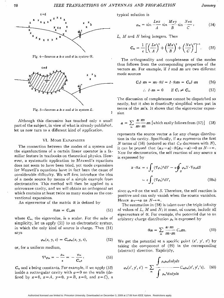
C, and E being constants. For example, if we apply (53) inside a rectangular cavity with p=O on the walls (defined by x = O , x = A , y=O, y = B , z = O , and z=C) , a

e CRLE

typical solution is

LTX Mlry L V T 2 ym = sin - sin - sin - 7

A B C (54)

L, M and N being integers. Then

The orthogonality and completeness of the modes thus follows from the corresponding properties of the vectors m. For example, if I and m are two different mode sources

The discussion of completeness cannot be dispatched so neatly, but it also is drastically simplified when put in terms of the m’s. I t shows that the eigenvector expansion

a = C - a . m m [which easily follows from (57)] (58)

m.m

represents the source vector a for any charge distribution in the cavity. Specifically, if a.v represents the first N terms of (58) (ordered so that CX decreases with AT), i t can be proved that (a:\- - a) . (R(aK -a) -0 as N+ Q). Xow for electrostatics, the self reaction of any source x is expressed by

since pz=O on the wall S. Therefore, the self reaction is positive and can only vanish when the source vanishes. Hence a.%r-a as AT- a.

The summation in (58) is taken over the triple infinity of values of L, M and N ; it must, of course, include all eigenvectors of @. For example, the potential due to an arbitrary charge distribution pa is expressed by

m = C - a . m Cmm .

, m.m (59)

We get the potential a t a specific point (x’, y‘, 2’) b y taking the component of (59) in the corresponding (abstract) direction. Explici.tly,


1963 Rumsey: Solz.ing Advanced Problems in Electromagneiic Fields 79

Kotice how this method directly leads to an explicit solution for this rather advanced type of problem, for pa is given, the pm’s are explicit functions and the C,’s are explicit constants.

The summation over L, X , and :V converges slowly if the source occupies a small fraction of the cavity. For example, in the extreme case of a point source, this method is impractical for representing the field near the source; the method of images is then much more suit- able, as we shall see at the end of Section VIII. It should be noted, however, that the mode expansion derived from the eigenvector definition (51) can easily be adapted to take into account the fact that the source is confined to a small region, and so to yield a more con- vergent series. To illustrate this, suppose that the source pa is known to vanish outside of the range (x&. Then n7e limit the pm’s so that they also vanish outside of ( ~ 1 x 2 ) ; in other words, only the points in (xlxp) now constitute the basis for the vectors m. Thus pm now satisfies the source-free equation in the ranges (0x1) and (xza) , but in (x1x2) p, satisfies the eigenvector condition (53). Then continuity of p,,, and dp,/dx a t x1 and x2 again yields a discrete set of C,’s and corresponding m’s , and because the m’s fit (51), the standard mode expansion still applies. The specific formulas for our electrostatic example can be written as follows:

M7ry P,(ye) = sin -- sin -

B C

In (Oxl) pm = P,s/zTxF,(yz).

In (x1x2)

pm = sin (u,x + 6,)F,(yz).

In ( x ~ u )

pm = Q,s/z( T X - a)F,(yz),

where .On, is given by the following equation for urn:

tan 6, = u,,tkTrl - T tan ztmxl

T + .u,thTxl tan umxl

zimthT(x2 - e) - T tan ztx2

T + zt,tkT(r~ - e) tan U,EZ

sin (u,R-.~ + 6,) - -

P, = sh T x ~

sin (u,x2 + 8,) Qm =

SIZT(U - 2 2 )

and the eigenvalue

1 c, = - [T’ + ztm’]-’. E

The unit voltage source used in Section VI11 [see (Sl)] is an application of this method to the extreme case where the volume between.the planes x1 and x 2 shrinks to a plane.

Let us now apply the same abstract formulas to mi- crowaves generated by an arbitrary source in a cavity. To ensure that the field of this source is unique, the frequency must not coincide with any of the resonances of the cavity, if a = 0. If a# 0, uniqueness is ensured a t all frequencies. The eigenvector equation (51) now says, according to (34) and (33 ,

H, = - C,K, and E, = CnJn. (61)

Suppose, for simplicity, that the medium which fills the cavity is homogeneous, and that tangential E vanishes on the walls. Then the Rlaxwell equations (19) and (20), when combined with (61), give

Cn?(P,,? - WZpE + j,,,) + CJjwp - j w c - u) - 1 = 0

for P n # 0, (62)

where 0, is one of the mode numbers determined from the boundary conditions applied to

V x V X E, = Pn2En and V x V x H, = PnPHn. (63)

Maxwell’s equations show also that we can take E, real and H, pure imaginary. If cr = 0, Pn2 = w,2pe, where w n is a resonance frequency. For example, when the cavity is rectangular, as in the preceding paragraph,

In this case there are four modes corresponding to one value of Pn [and, as (64) indicates, there will be many more than four if any two of the lengths A , B and C are commensurate]. This quadrupling effect comes from a doubling due to (62) and a doubling due to (63). The former is due to the fact that (62) is a quadratic for C,, thus giving two C,’s for one 0%. The latter is due to the fact that a complete set of solutions of (63) can be com- posed from a transverse electric (TE) set and a transverse magnetic set (TM) [2].

As we have seen, (62) does not apply if Sn = 0. Going back to the definition of a mode source in (61), we see from Maxwell’s equations that a possible mode, denoted now by subscript q, is represented by

E, = 0 J, = 0 and j ~ p H , = - K,, (65)

with

V X H, = 0. (66)

This fits the boundary condition NXE,=O and the mode definition (61), as well as Maxwell’s equations. Moreover, it is orthogonal to all the modes with &#0, for the simple reason that C, is different from any of the Cn’s [see (57)]. Evidently there is an analo-


80 IEEE TRANSACTIONS ON ANTENNAS AND PROPAGATIOhr Januarg

gous set of modes, denoted by subscript 9, such that

H, = 0, K, = 0, (jue + u)E, = J, (67)

and

V X E = O , (68)

but with the additional restriction that

N X E, = 0, on S.

Obviously q - p = 0. Hence the p - , p-, and n-mode types are orthogonal.

Just as a complete set of the n modes is given by all the solutions of (63) with NXE,=O, so a complete set of p modes is given by all the solutions of (66). Instead of giving the usual set of eigenfunctions, this gives merely

H, = VV,, (69)

where V , is an arbitrary scalar. Note that V, does not have to satisfy any specific boundary condition at S in order to make NXE,=O because all q modes have E,= 0 everywhere. However, since the field of an arbitrary source a satisfies the boundary condition N .H, =0, we make

N . VV, = 0, on S. (71)

Since

let us say, we get a complete set of 17,'s by setting

s, = A,V,

(where A is a constant) and by applying (71). Thus for the rectangular cavity we can take

v, = cos - L m M n y ATnz

A B C cos - cos - * (72)

I t is clear that the modes can be expressed in a similar way, but in this case

E, = VVs, (73) with

V 8 = 0, on S. (74)

We are now in a position to write the field of an arbitrary source a in the cavity, by means of the standard form (59). The summation over the m ' s is now replaced by summation over six types of mode, the four n types, the p types, and the q types. The terms in (58) are given explicitly as follows (m stands for any of the n's, p ' s , or q 's ) :

a . m = Jv(Jn* Jm + K*Km)dV, (75)

= Jv(Jm2 + Km2)dV* (76)

and the Cm's are given by (62) or (65) or (67). Thus, for the electric field, (59) gives

For example, to find the field due to a probe which pro- jects through a hole in the wall of the cavity, we substi- tute the current on the metal part of the probe for Ja,

and the equivalent magnetic current E,XN, derived from the electric field in the hole, for K,.

For lossless cavities it may be more convenient to use a set of modes for which either J = 0 or K = 0; in other words, a combination of purely magnetic or purely electric modes. By comparison, note that each individual mode obtained from (61) is itself a combination of electric and magnetic types. The advantage of the pure types is that for J =0, K, and E, can be taken pure real, and H, pure imaginary (provided u=O), and corre- spondingly for the type with K, = 0. Note that this also applies to the p - and q-mode types. Thus n.n is always positive real and can be set equal to unity. The eigen- values C, also take a simpler form,

VII. THE CONNECTION BETWEEN CIRCUIT THEORY AND FIELD THEORY

The definitions of reaction make a . the same physical entity in field theory and in circuit theory. Hence the difficult problem of connecting the two theories is automatically accomplished. For example, (23) shows that the current passing between the nth pair of terminals due to source b is the reaction of b on a unit voltage source connected across the terminals, ;.e.,

a - a b = I b , (7 8>

if a is a unit voltage source and Is the current through it due to source b. To see how the same result comes from field theory, in (21) and (22) let a denote a unit voltage source connected to some antenna. This means that a must consist of a sheet of magnetic current distributed in solenoidal form around a cylinder of perfect electric conductor. Since tangential E vanishes a t the surface of this cylinder, and is discontinuous on passing through the magnetic current sheet by an amount equal to the surface current density, tangential E just outside the solenoid is equal to the surface current density turned through a right angle. Therefore, if the cylinder is infinitesimal (in length and diameter), the magnetic current sheet produces a voltage between its ends which is independent of the environment. kloreover, the passive impedance between these ends is zero. Thus the magnetic current solenoid with electrically conduct-


1963 Rumsey: Solving Advanced Problem i.n Electromagnetic Fields 81

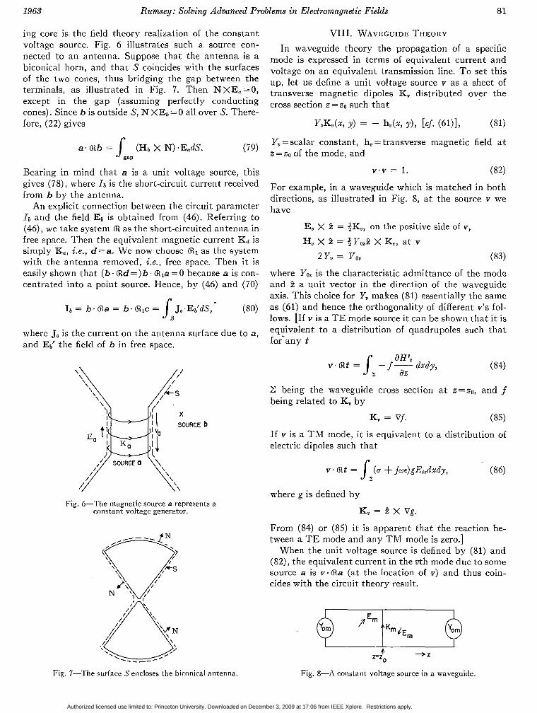
ing core is the field theory realization of the constant voltage source. Fig. 6 illustrates such a source connected to an antenna. Suppose that the antenna is a biconical horn, and that S coincides with the surfaces of the two cones, thus bridging the gap between the terminals, as illustrated in Fig. 7. Then NXE, =0, except in the gap (assuming perfectly conducting cones). Since b is outside S, N XEb = 0 all over s. There- fore, (22) gives

a * ab = (Hb X N) *E,dS. Lap (79)

Bearing in mind that a is a unit voltage source, this gives (78), where Ib is the short-circuit current received from b by the antenna.

An explicit connection between the circuit parameter I b and the field E6 is obtained from (46). Referring to (46), we take system &t as the short-circuited antenna in free space. Then the equivalent magnetic current Ka is simply K,, ;.e., d=a . We no~7 choose (R1 as the system with the antenna removed, ; .e. , free space. Then it is easily shown that (b. Qld=)b. ala = 0 because a is con- centrated into a point source. Hence, by (46) and ( T O )

"

Ib = b. @a = b . (R~c = Jc.E:dS, JS (80)

where Jc is the current on the antenna surface due to a, and E{ the field of b in free space.

Fig. +The magnetic source a represents a constant voltage generator.

Fig. 7-The surface S encloses the biconical antenna.

VIII. WAVEGUIDE THEORY In waveguide theory the propagation of a specific

mode is expressed in terms of equivalent current and voltage on an equivalent transmission line. To set this up, let us define a unit voltage source v as a sheet of transverse magnetic dipoles K, distributed over the cross section z = zo such that

FJL(r, y ) = - h*(x, >I), [cj. (61)], (81)

I!, =scalar constant, h, =transverse magnetic field a t z = Z O of the mode, and

V'V = 1. (82)

For example, in a waveguide which is matched in both directions, as illustrated in Fig. 8, a t the source v we have

E, X 3 = $Kz, on the positive side of v, H, X 3 = $P& X K,, at v

2 I', = Yo0 (83)

where Yo, is the characteristic admittance of the mode and 5 a unit vector in the direction of the waveguide axis. This choice for Y, makes (81) essentially the same as (61) and hence the orthogonality of different v's follows. [If v is a TE mode source it can be shown that it is equivalent to a distribution of quadrupoles such that f o i a n y t

Z being the waveguide cross section a t z=zo, and f being related to K, by

K, = Vj. (85)

If v is a TM mode, i t is equivalent to a distribution of electric dipoles such that

V' at = (u + jW€)gEl,drdy, L (86)

where g is defined by

K, = 2 x Vg. From (84) or (85) i t is apparent that the reaction between a TE mode and any T M mode is zero.]

When the unit voltage source is defined by (81) and (82), the equivalent current in the vth mode due t o some source a is v - @a (at the location of v) and thus coincides with the circuit theory result.

z=zo a -+z

Fig. 8-A constant voltage source in a waveguide.


82 IEEE TRANSACTIONS ON ANTENATAS AhlD PROPAGATION January

Similarly, the unit mode current source a t z=za consists of the electric dipoles Ji defined by

ZiJi(z, y ) = ei(x, y), the transverse electric field (87)

a t z=za of the mode, and i . i=l . Then the equivalent mode voltage at i due to source a is -i. @a. In summary then, if a is any source, its mode voltage and cur-

OPEN CIRCUIT

I I I

PORT 2

rent for some mode m are

Vam(zo) = - i. @a

I,,(zo) = v - a a

CIRCUIT OPEN --t+-pPORT, (88)

(89) Fig. 9--.4 unit current source i in system a.

the unit current and voltage sources i and v being placed at z = zo.

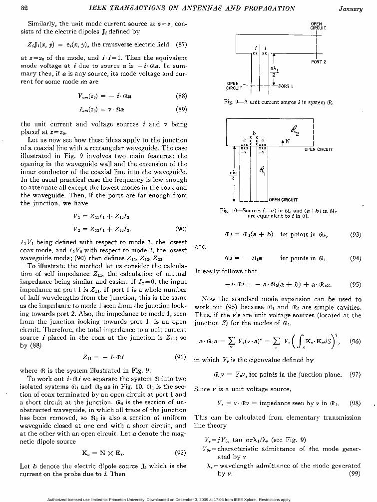
Let us now see how these ideas apply to the junction of a coaxial line with a rectangular waveguide. The case illustrated in Fig. 9 involves two main features: the opening in the waveguide wall and the extension of the inner conductor of the coaxial line into the waveguide. In the usual practical case the frequency is low enough to attenuate all except the lowest modes in the coax and the waveguide. Then, if the ports are far enough from the junction, we have

v1 = 21111 + 2 1 2 1 2

v 2 = 2 1 2 1 1 + 2 2 2 1 2 , (90)

I I V 1 being defined with respect to mode 1, the lowest coax mode, and 12V2 with respect to mode 2, the lowest waveguide mode; (90) then defines 211, 2 1 2 , 2 2 2 .

T o illustrate the method let us consider the calculation of self impedance Zll, the calculation of mutual impedance being similar and easier. If 12 = 0, the input impedance a t port 1 is 211. If port 1 is a whole number of half wavelengths from the junction, this is the same as the impedance to mode 1 seen from the junction looking towards port 2. 4 1 ~ 0 , the impedance to mode 1, seen from the junction looking towards port 1, is an open circuit. Therefore, the total impedance to a unit current source i placed in the coax at the junction is Zll; so by (88)

CIRCUIT

Fig. 1GSources (-a) in @I and (afb) in are equivalent to i in @.

CRi = @*(a + b) for points in @2, (93)

and & * = - la for points in (ill. (94)

I t easily follows that

-i. &' = - a . &(a + b) + a- ala. (95)

Now the standard mode expansion can be used to work out (95) because, 6i1 and I R 2 are simple cavities. Thus, if the v's are unit voltage sources (located at the junction .S) for the modes of R1,

(91) in which Y,, is the eigenvalue defined b y

where 6i is the system illustrated in Fig. 9. To work out i- ai we separate the system @ into two

C&v = Y J , for points in the junction plane. (97)

isolated systems @I and @z as in Fig. 10. @ I is the sec- since is a unit voltage source, tion of coax terminated by an open circuit at port 1 and a short circuit at the junction. (Rz is the section of un- Y, = v - @v = impedance seen by v in (98) obstructed waveguide, in which all trace of the junction has been removed, so is also a section of uniform This can be calculated from elementary transmission waveguide closed a t one end with a short circuit, and line theory at the other with an open circuit. Let a denote the magnetic dipole source Y, = j YO, tan n ~ h l h (see Fig. 9)

K, = N X Et. (92) Yo, =characteristic admittance of the mode gener-

ated by v Let b denote the electric dipole source Jb which is the X, =wavelength admittance of the mode generated current on the probe due to i. Then by Y. (99)


1963 Rumey: Solving Advanced Problems in Electromagnetic Fields 83

Likewise if the u ’ s are unit volume mode sources for @z, like the m’s in (56) to (7i) but now u * u = ~ ,

a . @.(a + b) = C,u.a(u.a + u.b ) = cu U U

Here S’ is the surface of the probe and the eigenvalue C, is the same entity as C, in (56) to (77) (it is different numerically because one wall of az is an open circuit whereas C, was defined for short-circuit boundary conditions on all walls).

On combining (91), ( 9 3 , (96), and (loo), we get a formula for Zll expressed in terms of the tangential electric field in the opening (;.e., a) and the current on the probe (ie., b). These can often be estimated with good accuracy so the problem is solved in such cases, especially in view of the variational properties of the formula which we shall discuss later on. To set up the proper variational form we need to fix the lengths of a and b relative to i. S o w since the tangential electric field vanishes on the probe,

b . &(a 4- b) = 0, (101)

which fixes the length of b relative to a. Also, i t is easily shown that if

K, = N X Ji, (101a) a . r = - i. ai (101b)

which fixes the length of a relative to i. Hence

(a . r )? (a.@b)%

Zll b. RZb

Evidently this gives Zll independently of the lengths of a and 6. The series expansions for all except b . @*b are given in (96) and (100) from which that for b . a& is apparent.

T o get an exact solution we need to find the current on the probe and the electric field in the opening, due to the unit current source i in Fig. 9. Let us then introduce, in addition to the set { v } of unit voltage sources in a1 and the set { u ) of unit volume sources in a ~ , t h e set { d } of orthogonal u n i t vectors which represent a complete set of surface current distributions on S’, the surface of the probe.

Then we can write

-- - a . ala - a - &a + . (101c)

a = C a - v v (102)

b = b . d d (103)

V

d

and the problem is to find the coefficients a * v and b. d. We also have

d = d . u u (104) U

v = V ’ U U (105) U

in which the coefficients d . u and v-u are known. Let r be the particular member of ( v f which generates the same mode as that generated by i so that

K, = N X Ji as in (101a). (106)

Let 6,GO if r # v , and 6,, 4 1. Then i t is easily shown from (106) tha t

6,, = Y,v.a + V - U C ~ U

‘( d u - d d - b + u.v’v’-a . (107) V’ )

Since tangential E , + E b = O on S’,

d - &(a + b) = 0, (108)

which gives

d.uC,( u.vv.a + u.d’d’-b = 0. (109)

U u d’ ) Kow (107) holds for all v and (109) for all d. These two equations therefore are sufficient to determine the a . v’s and b . d’s.

The mode expansion converges satisfactorily for a thick probe, but for a thin one it may be better to use the method of images. For example, b in is equivalent to b+bl+bz . . . in free space (&), bl, bz, . . . being the images of b in the waveguide walls. The singu- larity associated with the thin probe is then contained in the single term b . @oa or b. a&, whereas it enters in every term of the mode expansion.

IX. ANTENNA PATTERN CALCULATIOXS

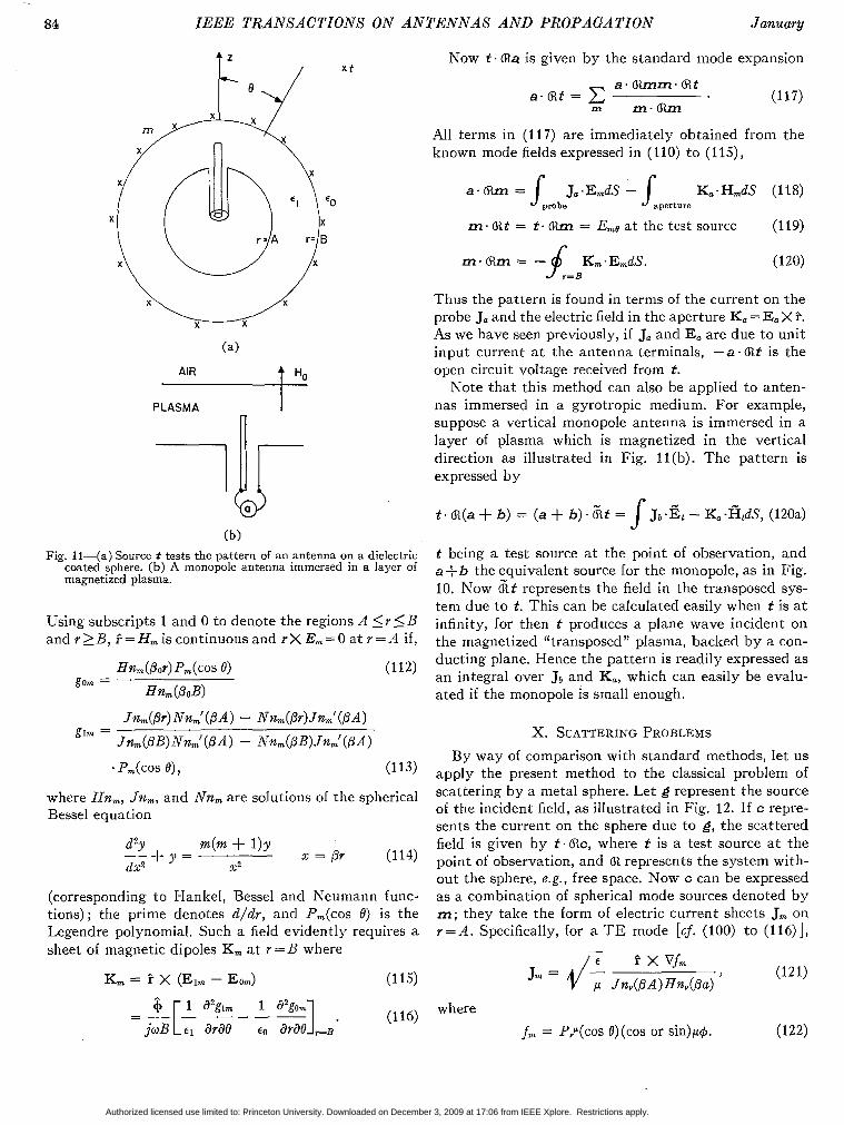
To illustrate how the abstract method greatly simplifies antenna calculations, suppose we wish to find the pattern of some antenna which is near a metal sphere coated with a layer of dielectric. Fig. ll(a) illustrates the case where the antenna is a coaxial probe aligned along a radius. Its radiation pattern is found by evaluat- ing the reaction of the source of the field transmitted by the antenna, denoted by a on a test source t at infinity. If n7e adopt a conventional set of spherical coordinates Y , O , C $ , we get E,# by taking t as an electric dipole of unit current moment placed parallel to 6. To accomplish this, we replace a by a combination of spherical mode sources m located on the surface of the dielectric r = B. Now in this problem i t is clear that the field is uniform around the axis of the coaxial probe, the z axis, and is T M with respect to it. Therefore, we need consider only T M modes independent of C$. These modes are expressed by the formulas

H, = V X Pg,,,, i. = unit radial vector (110)

jw&, = v x B x fgm = v + p*i.g,. (111)


84 IEEE TRANSACTIONS O N AhTTEhTNAS AND PROPAGATION January

x t

(b) Fig. 11-(a) Source t tests the pattern of an antenna on a dielectric

coated sphere. (b) A monopole antenna immersed in a layer of magnetized plasma.

Using subscripts 1 and 0 to denote the regions A I r 5 B and r >_ B, i = Hm is continuous and r X E, = 0 a t r = 4 if,

Now t . &a is given by the standard mode expansion

a - R t = (117) a . Ciimm. R t

m m- (Rm

rzll terms in (1 17) are immediately obtained from the known mode fields expressed in (1 10) t o (1 15),

= S,nac J,.EmdS - K,-H,dS (118)

m- R t = f . (Rm = E,,o at the test source (119) aperture

Thus the pattern is found in terms of the current on the probe J, and the electric field in the aperture K, =E, X 1. As we have seen previously, if J, and E, are due to unit input current at the antenna terminals, --a. at is the open circuit voltage received from f .

Kote that this method can also be applied to antennas immersed in a gyrotropic medium. For example, suppose a vertical monopole antenna is immersed in a layer of plasma which is magnetized in the vertical direction as illustrated in Fig. ll(b). The pattern is expressed by

t being a test source at the point of observation, and a+& the equivalent source for the monopole, as in Fig. 10. Now 6 i f represents the field in the transposed system due to f. This can be calculated easily when t is at infinity, for then t produces a plane wave incident on the magnetized “transposed” plasma, backed by a con-

where Hn,, Jn,, and Nnm are solutions of the spherical Bessel equation

(corresponding to Hankel, Bessel and Neumann functions); the prime denotes d / d r , and P,(cos 0) is the Legendre polynomial. Such a field evidently requires a sheet of magnetic dipoles K m at r = B where

Km = 1 X ( E l m - EO^) (115)

(116)

(112) ducting plane. Hence the pattern is readily expressed as an integral over Jb and K,, which can easily be evaluated if the monopole is small enough.

X. SCATTERING PROBLEMS By way of comparison with standard methods, let us

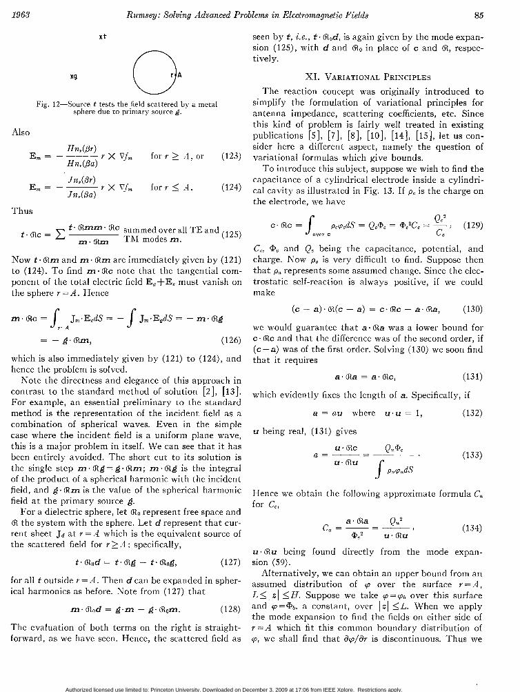
apply the present method to the classical problem of scattering by a metal sphere. Let g represent the source of the incident field, as illustrated in Fig. 12. If c represents the current on the sphere due to g, the scattered field is given by f . @c, where f is a test source a t t he point of observation, and @ represents the system with- out the sphere, e.g., free space. Now c can be expressed as a combination of spherical mode sources denoted by m; they take the form of electric current sheets Jm on r =.4. Specifically, for a TE mode [c j . (100) to (116) 1,


1963 Rumsey : So1vin.g Adz:anced Problem in Electromagnetic Fields 85

x t

W Fig. 12-Source f tests the field scattered b y a metal

sphere due to primary source g.

Also

Thus

t - a c = f' @mm. ac summed over all TE and m. TM modes m. (125)

Now t.(Rm and m-(Rm areimmediatelygiven by (121) to (124). T o find m. (Rc note that the tangential component of the total electric field E,+E, must vanish on the sphere Y =A. Hence

M . RC = J J ~ . E , ~ S = - J J~.E,~s = - m . ag r=.4

= - g.crjn, (126)

which is also immediately given by (121) to (124), and hence the problem is solved.

Xote the directness and elegance of this approach in contrast to the standard method of solution [2] , [IS]. For example, an essential preliminary to the standard method is the representation of the incident field as a combination of spherical waves. Even in the simple case where the incident field is a uniform plane wave, this is a major problem in itself. We can see that it has been entirely avoided. The short cut to its solution is the single step m. (Rg=g. (Km; m - (Kg is the integral of the product of a spherical harmonic with the incident field, and g - (Rm is the value of the spherical harmonic field at the primary source g.

For a dielectric sphere, let 6 i o represent free space and (R the system with the sphere. Let d represent that current sheet Jd a t Y = A which is the equivalent source of the scattered field for Y >A : specifically,

t . (Rod = t . 6tg - f. a&, (125)

for all f outside Y = 4 . Then d can be expanded in spherical harmonics as before. Note from (127) that

m.(Rod = g . m - g.(Rom. (128)

The evaluation of both terms on the right is straight- forward, as we have seen. Hence, the scattered field as

seen by t , i e . , t . (Rod, is again given by the mode expansion (125), with d and (Ro in place of c and (R, respectively.

XI. VARIATIONAL PRIXCIPLES The reaction concept was originally introduced to

simplify the formulation of variational principles for antenna impedance, scattering coefficients, etc. Since this kind of problem is fairly well treated in existing publications [5], [7], [8], [ lo] , [14], [IS], let us consider here a different aspect, namely the question of variational formulas which give bounds.

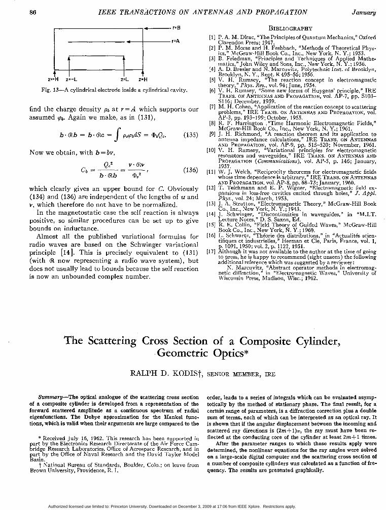
T o introduce this subject, suppose we wish to find the capacitance of a cylindrical electrode inside a cylindrical cavity as illustrated in Fig. 13. If pc is the charge on the electrode, we have

S Q C 2

c.(Rc = pcpcdS = QeaC = @c2Cc = - J (129) over c c c

C,, CP, and Qe being the capacitance, potential, and charge. Now pc is very difficult to find. Suppose then that pa represents some assumed change. Since the electrostatic self-reaction is always positive, if we could make

(c - a ) . (R(c - a ) = c - Rc - a . (Ra, (130)

we would guarantee that a . (Ra was a lower bound for c . a c and that the difference was of the second order, if ( c -a) was of the first order. Solving (130) we soon find that it requires

a. 6ia = a. (Rc, (131)

which evidently fixes the length of a. Specifically, if

a = a u where u ' u = 1, (132)

u being real, (131) gives

Hence we obtain the following approximate formula C, for C,,

(134)

u - (F(u being found directly from the mode expansion (59).

4lternatively, we can obtain an upper bound from an assumed distribution of cp over the surface Y = B , L 5 I zI SH. Suppose we take p = y b over this surface and q = @ b , a constant, over I z I SL. When we apply the mode expansion to find the fields on either side of r = A which fit this common boundary distribution of y, we shall find that dy,-/dr is discontinuous. Thus we


86 IEEE TRANSACl’IONS ON ANTENNAS AXD PROPAGATION January

I t t 2z-H z=-L z=L z=H

Fig. 13-A cylindrical electrode inside a cylindrical cavity.

find the charge density P b a t r = A which supports our assumed (db. Again we make, as in (131),

b . ab = b. @C = p,pbdS = @ b Q c . (135) S Now we obtain, with b = bv,

which clearly gives an upper bound for C. Obviously (134) and (136) are independent of the lengths of u and v , which therefore do not have to be normalized.

In the magnetostatic case the self reaction is always positive, so similar procedures can be set up to give bounds on inductance.

Almost all the published variational formulas for radio waves are based on the Schwinger variational principle [14]. This is precisely equivalent to (131) (with now representing a radio wave system), but does not usually lead to bounds because the self reaction is now an unbounded complex number.

BIBLIOGRAPHY [I] P. A. &I. Dirac, “The Principles of Quantum Mechanics,” Oxford

[2] P. M . Morse and H. Feshbach, “Methods of Theoretical Phys- Clarendon Press; 1947.

[3] B. Friedman, “Principles and Techniques of A plied Mathe- ics,” McGraw-Hill Book Co., Inc., New York, N. Y.; 1953.

[4] A. D. Bresler and N. Marcuvitz, Polytechnic Inst. of Brooklyn, matics,’John Wiley and Sons, Inc., New York, 8 Y . ; 1956.

Brooklyn, K. Y., Rept. R495-56; 1956. [j] V. H. Rumsey, “The reaction concept in electromagnetic

[6] V. H. Rumsey, “Some new forms of Huygens’ principle,” IRE theory,” Pkys. Rev., vol. 94; June, 1954.

TRANS. ON ANTEKNAS AND PROPAGATION, vol. AP-7, pp. S103- S116; December, 1959.

[7] M. H. Co$n, “Application of the reaction concept to scattering problems, IRE TRASS. ON ANTENNAS ?LND PROPAGATION. vol. AP-3. DO; 193-199: October. 1955.

[8] R. F: *Harrington ‘:“Time Harmonic Electromagnetic Fields,” McGraw-Hill Book Co., Inc., New York, N. Y.; 1961.

[9] J. H. Richmond, “ A reaction theorem.and its application to antenna impedance calculations,” IRE TRANS. ON ANTENNAS AND PROPAGATION, vol. AP-9, pp. 515-520; November, 1961.

[lo] V. H. Rumsey, “Variational principles for electromagnetic resonators and waveguides,” IRE TRAHS. ON ANTENNAS AND PROPAGATION (Commzrtaications), vol. AP-5, p. 146; January, 1957 %‘: J. Welch, “Reciprocity theorems for electromagnetic fields whose time dependence is arbitrary,” IRE TRaNs. ON ANTENNAS AXD PROPAGATION. vol. AP-8, pp. 68-23; January, 1960. T. Teichmann and E. P. Wigner, Electromagnetic field expansions in loss-free cavities excited through holes,” J. Appl .

J. A. Stratton, “Electromagnetic Theory,” McGraw-Hill Book Phys., vol. 24; March, 1953.

J. Schwmger, “Discontinuities in waveguides,” in “M.I.T. Co., Inc.,, New York, N. Y . ; 1943.

Lecture Kotes,” D. S. Saxon, Ed. K. E. Collin, “Field Theory of Guided Waves,” McGraw-Hill Book Co., Inc., New York, N. Y. ; 1960. L. Schmartz, “The‘orie des distributions,” in “Actualitb scien- tifiques et industrielles,” Herman et Cie, Paris, France, vol. 1, p. 1091, 1950; vol. 2, p. 1122, 1951. Although it was not available to the author a t the time of going to press, he is happy to recommend (sight unseen) the following additional reference which was suggested by a reviewer:

netic diffraction,” in “Electromagnetic Waves,’’ University of N. Marcuvitz, ”Abstract operator methods in electromag-

Wisconsin Press, PIadison, Wisc.; 1962.

The Scattering Cross Section of a Composite Cylinder, Geometric Optics*

Summary-The optical analogue of the rcattering cross section of a composite cylinder is developed from a representation of the forward scattered amplitude as a continuous spectrum of radial eigenfunctions. The Debye approximation for the Hankel functions, which is valid when their arguments are large compared to the

part by the Electronics Research Directorate of the Air Force Cam- * Received July 16, 1962. This research has been supported in

bridge Research Laboratories, Office of Aerospace Research, and in part by the Office of Naval Research and the David Taylor Model Basin.

t Kational Bureau of Standards, Boulder, Colo.; on leave from Brown University, Providence, R. I.

order, leads to a series of integrals which can be evaluated asymp- totically by the method of stationary phase. The hal result, for a certain range of parameters, is a diffraction correction plus a double s u m of terms, each of which can be interpreted as CUI optical ray. I t is shown that if the angular displacement between the incoming and scattered ray directions is ( 2 m + l ) ~ , the ray must have been re- flected at the conducting core of the cylinder at least 2m+l times.

After the parameter ranges to which these results apply were determined, the nonlinear equations for the ray angles were solved on a large-scale digital computer and the scattering cross section of a number of composite cylinders was calculated a s a function of frequency. The results are presented graphically.


Documents

A Short Way of Solving Advanced Problems in ... · A Short Way of Solving Advanced Problems in Electromagnetic Fields and Other Linear Systems* V. H ... tering and antenna problems,