A Sigma-Point Kalman Filter for remote sensing of updrafts ... · PDF fileA Sigma-Point Kalman Filter for remote sensing of updrafts in ... a certain decay and rebirth ... for remote

A Sigma-Point Kalman Filter for remote sensingof updrafts in autonomous soaring

Martin Stolle, Yoko Watanabe and Carsten Doll

Abstract Autonomous soaring is a promising approach to augment the endurance ofsmall UAVs. Most of the existing work on this field relies on accelerometers and/orGPS receivers to sense thermals in the proximity of the vehicle. However, thermalupdrafts are often visually indicated by cumulus clouds that are well characterizedby their sharp baselines. This paper focuses on a cloud mapping algorithm whichestimates the 3D position of cumulus clouds. Using the meteorological fact of auniform cloud base altitude a state-constrained sigma-point Kalman filter (SCSPKF)is developed. A method of using the resulting cloud map and its uncertainty in thepath planning task to realize a soaring flight to a given wayoint is presented as aperspective of this work.

1 Introduction

Accelerated by a breakthrough in micro electromecanical systems (MEMS), smallUAVs and the role they play in our society, be it military or civil, have grown inimportance in the near past. However, their utility is still restricted due to small pay-load capacities as well as poor endurance and small operational ranges. One existingidea to overcome these still predominant drawbacks, is to apply flight control andguidance algorithms for soaring flight [1, 2, 3]. The soaring flight makes use of up-drafts to lift the UAV and hence to reduce the transported mass dedicated to energy(battery or fuel). Moreover, soaring UAVs operate silently which clearly is a benefitfor military purposes.

Martin Stolle · Yoko Watanabe · Carsten DollDepartment of Systems Control and Flight Dynamics (DCSD), The French Aerospace Laboratory(ONERA),2 avenue Edouard Belin, 31055 Toulouse Cedex 4, Francee-mail: [email protected],[email protected],[email protected]

1

2 Martin Stolle et al.

Generally speaking, soaring flight combines all kind of techniques to keep an un-powered aircraft airborne. Dynamic soaring for instance is a technique where thevehicle harnesses energy from horizontal wind gradients. In thermal soaring energyis gained by relying on uprising currents of air. These buoyant plumes of rising airresult from gradients in the earth’s surface heating and can reach heights of up to4000m above ground according to [4]. In cross-country soaring, gliders fly beyondthe gliding distance from the initial take-off point performing waypoint navigation.Amongst existing approaches to automatic cross-country soaring, the work of Ed-wards et al. [5] is the only one which includes flight testing. His work lead to theparticipation in a cross-country soaring challenge for remotely piloted gliders andthe performance of a fully autonomous soaring flight over a distance of 50km. Withno a priori information about thermal locations in the far environment, the flightpath was defined as the direct line between two consecutive waypoints. The aircraftflight control mode was set to thermal centering mode, when encountering strongenough thermals on the path - detected by Inertial Measurement Unit (IMU) andGPS measurements. With this suboptimal flight path, the UAV could only benefitfrom a subset of possible updrafts - more precisely those that were directly locatedon the line of sight to a given waypoint. Evidently this approach is limited to con-ditions where a strong density of thermals is provided along the direct path and byconsequence carries a significant risk of mission failure.The author of [6] considered autonomous cross-country soaring from a top downapproach and proposed path planning algorithms assuming that a perfect map withpinpoint thermal locations is at hand which raises doubts about its applicability be-yond the synthetic case of computer simulations.Human glider pilot mostly rely on their vision to locate thermal updrafts indicatedby cumulus clouds. Doing so they can fly distances of up to 3000km. Inspired bythese performances, the paper on hand describes the development of an algorithmfor remotely sensing thermal updrafts by locating cumulus clouds. An increased un-certainty of a thermal position estimate can significantly augment the time the UAVwill spend on hitting the thermal and thus impacts the cross-country soaring perfor-mance. Therefore, the filter was designed to not only provide fast convergence butalso a confident estimation of the thermal position uncertainty. Finally, a perspec-tive is presented on how to take into account the uncertainty of estimated thermalpositions in the cost of a cross-country path planning algorithm.

2 Cumulus clouds and thermal updrafts

Consider a UAV flying in a sky that is partly covered by cumulus clouds. Dependingon their stage, these clouds are the most important visual indicator for thermals thatglider pilots rely on during thermal soaring.

A Sigma-Point Kalman Filter for remote sensing of updrafts in autonomous soaring 3

2.1 Thermals and their visible features

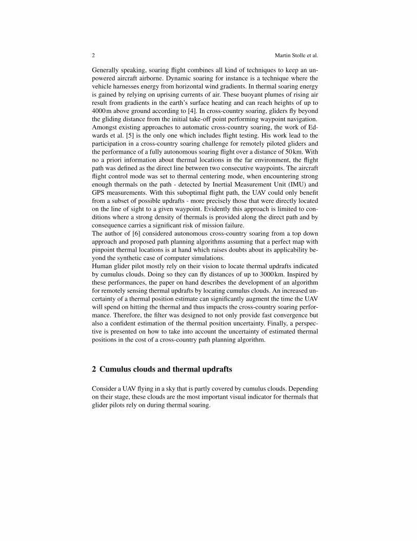
Vision-based object recognition algorithms detect objects in the real world from animage of the real world based on models. Since algorithmic description of this taskstill remains difficult, especially when dealing with objects such as clouds, varyingin shape, color and texture, most simple and informative features are to be used inorder to augment the recognition performance.Clouds that are based on thermals, in general undergo a certain decay and rebirthprocess consisting of two different stages. As long as a thermal source on the groundfeeds the cloud, it will continue growing and remains in the first building stage(fig. 1a). In case the thermal source vanishes, the cloud will start dying out (fig. 1b).The stages of a cumulus cloud are indicated by a variety of visible signs. For a grow-

(a) Growth (b) Decay

Fig. 1: Growth and decay of a cumulus cloud

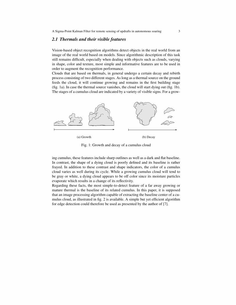
ing cumulus, these features include sharp outlines as well as a dark and flat baseline.In contrast, the shape of a dying cloud is poorly defined and its baseline is ratherfrayed. In addition to these contrast and shape indicators, the color of a cumuluscloud varies as well during its cycle. While a growing cumulus cloud will tend tobe gray or white, a dying cloud appears to be off color since its moisture particlesevaporate which results in a change of its reflectivity.Regarding these facts, the most simple-to-detect feature of a far away growing ormature thermal is the baseline of its related cumulus. In this paper, it is supposedthat an image processing algorithm capable of extracting the baseline center of a cu-mulus cloud, as illustrated in fig. 2 is available. A simple but yet efficient algorithmfor edge detection could therefore be used as presented by the author of [7].


Fig. 2: Baseline detection of a cumulus cloud

2.2 Dynamics of cumulus clouds

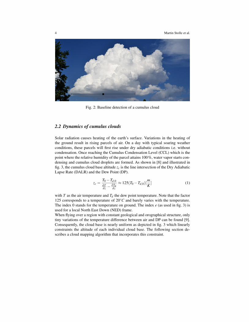
Solar radiation causes heating of the earth’s surface. Variations in the heating ofthe ground result in rising parcels of air. On a day with typical soaring weatherconditions, these parcels will first rise under dry adiabatic conditions i.e. withoutcondensation. Once reaching the Cumulus Condensation Level (CCL) which is thepoint where the relative humidity of the parcel attains 100%, water vapor starts con-densing and cumulus cloud droplets are formed. As shown in [8] and illustrated infig. 3, the cumulus cloud base altitude zc is the line intersection of the Dry AdiabaticLapse Rate (DALR) and the Dew Point (DP).

zc =T0−Td,0∂T∂ z −

∂Td∂ z

≈ 125(T0−Td,0)[mK] (1)

with T as the air temperature and Td the dew point temperature. Note that the factor125 corresponds to a temperature of 20◦C and barely varies with the temperature.The index 0 stands for the temperature on ground. The index e (as used in fig. 3) isused for a local North East Down (NED) frame.When flying over a region with constant geological and orographical structure, onlytiny variations of the temperature difference between air and DP can be found [9].Consequently, the cloud base is nearly uniform as depicted in fig. 3 which linearlyconstraints the altitude of each individual cloud base. The following section de-scribes a cloud mapping algorithm that incorporates this constraint.


(a) Cloud base definition(b) Cumulus clouds with uniform cloud base al-titude

Fig. 3: Dynamics of cumulus clouds

3 Cloud mapping algorithm

Combining the UAV’s state estimates with the output of the image processing al-gorithm, it becomes possible to estimate the 3D position of clouds in the inertialreference frame (index g). This problem is referred to as bearings-only target local-ization.

3.1 State definition and process model

With the cloud map containing the individual positions of all n clouds that are en-countered during a flight, the 3×n dimensional state vector x is defined as

x =[xT

1 xT2 . . . xn

T ]T (2)

where xi represents the cloud position of a single cloud in a local NED frame. Theindex g is not further carried for the sake of better readability. In general, the windvelocity has an effect on the drift of cumulus clouds, even if due to the inertia of thethermal air (note that the mass of a cumulus cloud can measure into the thousandsof tons), cumulus clouds drift much slower than the surrounding air. Therefore, weconsider a scenario with no cloud drift corresponding to weather conditions withonly little or no horizontal wind. This assumption is legitimate, since algorithmswill be tested on a small UAV glider whose flight envelope restricts operation to lowwind conditions. In that case, the state transition equation for a single cloud xi canbe modeled as


xi,k = f (xi,k−1)+wi,k−1 = xi,k−1 +wk−1 (3)

where w is the white and Gaussian process noise with covariance Q i.e.

w∼ w(0,Q) (4)

3.2 Measurement model

3.2.1 Pixel coordinates of cloud baseline’s center

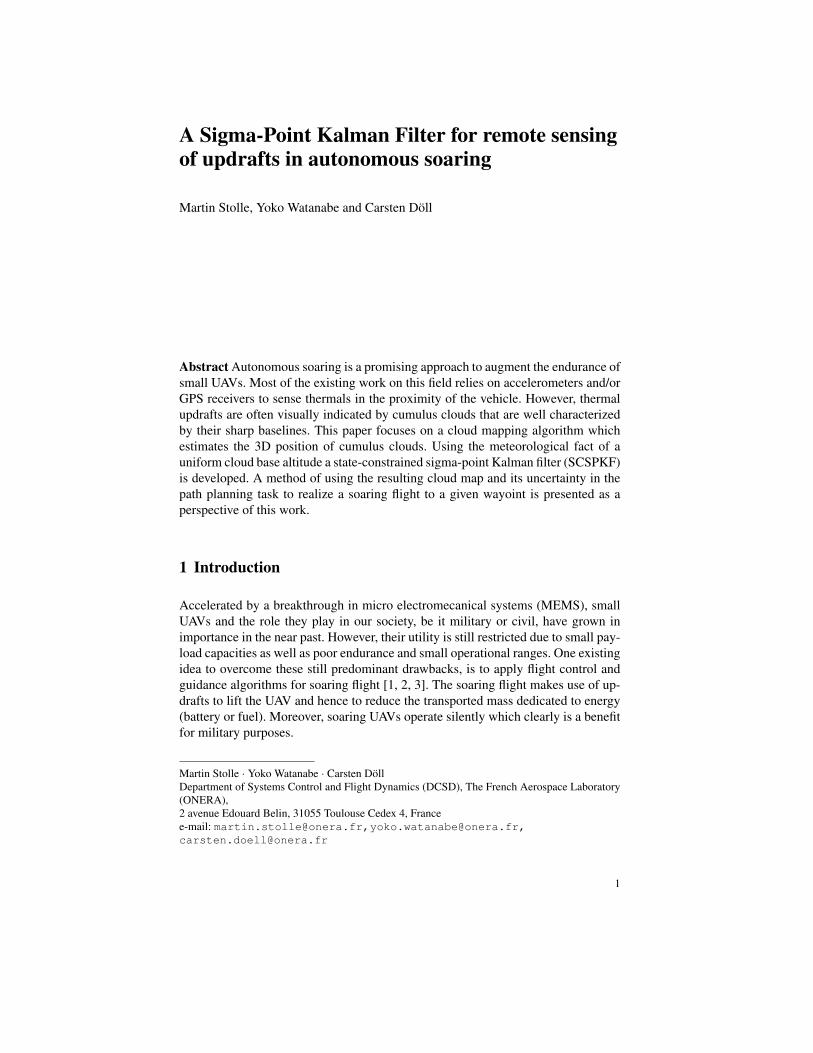
A forward looking camera is mounted on the UAV with a fixed offset from thevehicles center of gravity (CG) as well as a known angular offset from the body axis.At each time instance, the image processing algorithm outputs the center positionsof the m cumulus cloud baselines in the image resulting in a 2×m dimensionalmeasurement vector

yip =[yT

ip,1 yTip,2 . . . yT

ip,m]T

(5)

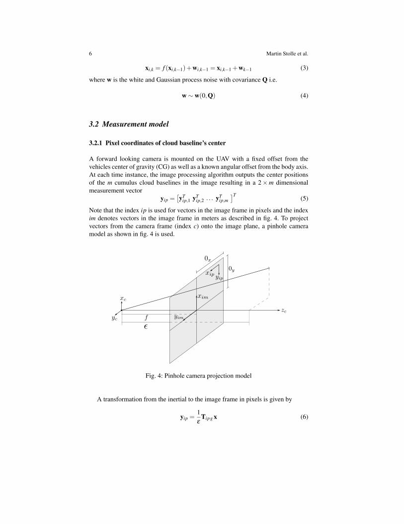
Note that the index ip is used for vectors in the image frame in pixels and the indexim denotes vectors in the image frame in meters as described in fig. 4. To projectvectors from the camera frame (index c) onto the image plane, a pinhole cameramodel as shown in fig. 4 is used.

Fig. 4: Pinhole camera projection model

A transformation from the inertial to the image frame in pixels is given by

yip =1ε

Tipg x (6)


where ε is the image depth. The transformation matrix Tipg includes the translationfrom the target to the vehicle Tvg, the rotation from the vehicle to the body frameTbv, the combined translation and rotation from the body to the camera frame Tcbas well as the combined projection and unit conversion (m to px) C from the cameraframe onto the image plane (see fig. 4)

Tipg = CTcbTbvTvg (7)

with the camera calibration matrix C being defined as

C =

[0 fx 0x 0− fy 0 0y 0

](8)

The two quantities fx and fy are function of the focal length f and the unit conver-sion factors Sx and Sy

fx =f

Sxand fy =

fSy

where the unit conversion is given by

Sx =yim

xip−0xand Sy =

xim

−yip−0y

Note that the parameters 0x and 0y are the offsets to the center of the image from theupper left hand corner.Adding Gaussian white measurement noise v, with zero mean and covariance R, thediscrete measurement equation is stated as

yk = h(xk)+vk =1ε

Tipg,kxk +vk = Hxk +vk (9)

Note that from here on the index of the measurement vector (ip) is not further carriedfor the sake of better readability.

3.2.2 Pseudo measurement for the altitude constraint

Significant filter performance augmentations can be reached when including the dy-namic relation between cloud base altitudes as a state constraint in the estimationprocess. Applied to the path planning, a faster convergence of position estimatesand covariances will as well invoke a faster reduction of the uncertainty ellipses.Consequently, the cross- country speed of the UAV glider increases, since less timewill be spent on encountering thermals.However, this benefit comes with a price. The assumption of a uniform cloudbaseis an approximation of the reality, and thus only a soft constraint where it is hard todetect constraints violations during estimation.To comprise the uniform cloud base state constraint, the 2×m dimensional mea-surement vector eq. (9) is augmented with the pseudo measurement d


ya =

[yd

]=

[HD

]x+[

vv1

](10)

where d is a null vector of dimension n and D is the n×3n-dimensional constraintmatrix with diagonal elements D1 =

[0 0 (1− 1

n )]

and off-diagonal elements D0 =[0 0 −1

n

]carrying the geometrical state restriction that the individual cloud bases zi

equals to the mean cloud base z. v1 is the white Gaussian noise of the state constraintwith covariance R1.

3.3 Estimation Algorithm

The bearings-only target localization is a highly nonlinear estimation problem. Avariety of nonlinear filters has been proposed to solve this problem. What is com-mon to nearly all of these methods, is the idea of providing a least squares estimateof the process’s state. The standard approach for nonlinear estimation is the Ex-tended Kalman Filter (EKF) that however comes with two significant drawbacks.Not only that the computation of the Jacobians is usually cumbersome, but if thelinearization is poor, the estimated state covariance will tend to be inconsistent andin the worst case overconfident as discussed in [10]. Projected to the problem ofautonomous cross-country soaring, this will erroneously tighten the error ellipsoidassociated to the estimated position of a cloud and potentially results in a thermalsearch within an area of sinking air.A common way to cope with this known weakness of the EKF is to artificially mag-nify the state covariance after each update or simply to drop certain observations.This is however an unfortunate and iterative procedure, since it discards informationthat is potentially useful.A main challenge of the bearings-only target localization is caused by its lack ofdepth-observability. With the trajectory having a significant impact on the observ-ability, there have been attempts [11] to design trajectories that optimize the targetobservability. However, in the case of autonomous cross-country soaring where theclouds are far away from the observing vehicle and the UAV aims to minimize en-ergy consumption, favoring target observability in the trajectory design is inefficient.More recently, a group of algorithms [12, 13, 14, 15] has been published to addressthe issues of the EKF by using deterministic sampling approaches circumventingboth laborious linearization and suboptimal performance due to poor linearizations.These algorithms referred to as sigma-point Kalman filters (SPKF) as well followthe prediction-correction procedure of the Kalman filter. But rather than linearizingthe nonlinear system equations, they use the intuition that it is easier to approximatea probability distribution than it is to approximate an arbitrary nonlinear function ortransformation. This is done by first propagating a weighted set of samples calledsigma points X through a nonlinear function. Then, the statistic properties of thepropagated state are recaptured. The principle behind this probability distributionapproximation is called Unscented Transform (UT) and was first presented in [12].


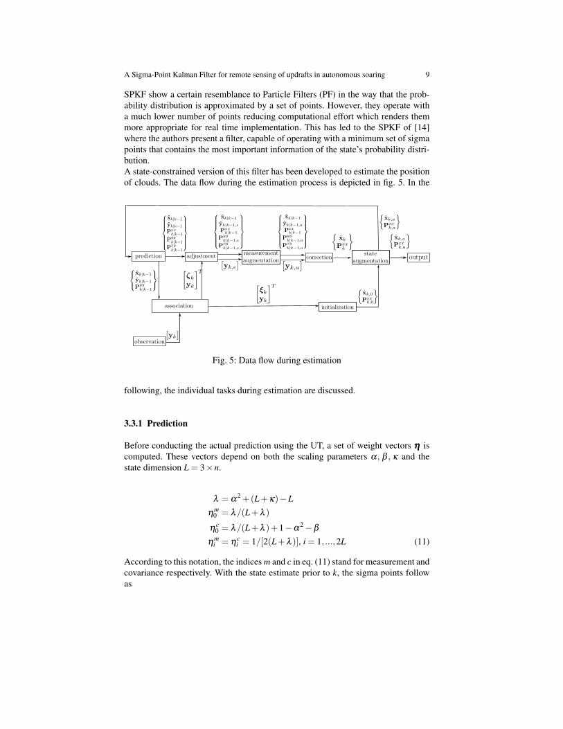
SPKF show a certain resemblance to Particle Filters (PF) in the way that the prob-ability distribution is approximated by a set of points. However, they operate witha much lower number of points reducing computational effort which renders themmore appropriate for real time implementation. This has led to the SPKF of [14]where the authors present a filter, capable of operating with a minimum set of sigmapoints that contains the most important information of the state’s probability distri-bution.A state-constrained version of this filter has been developed to estimate the positionof clouds. The data flow during the estimation process is depicted in fig. 5. In the

Fig. 5: Data flow during estimation

following, the individual tasks during estimation are discussed.

3.3.1 Prediction

Before conducting the actual prediction using the UT, a set of weight vectors ηηη iscomputed. These vectors depend on both the scaling parameters α, β , κ and thestate dimension L = 3×n.

λ = α2 +(L+κ)−L

ηm0 = λ/(L+λ )

ηc0 = λ/(L+λ )+1−α

2−β

ηmi = η

ci = 1/[2(L+λ )], i = 1, ...,2L (11)

According to this notation, the indices m and c in eq. (11) stand for measurement andcovariance respectively. With the state estimate prior to k, the sigma points followas


Xk−1 =[xk−1 xk−1 +

√L+λ

√Pxx

k−1 xk−1−√

L+λ√

Pxxk−1

](12)

Note that there are different approaches to compute the square root of a matrix.As suggested in [16], the lower Cholesky decomposition method is applied i.e.√

P = chol(P). Each of the sigma points X (i) is then propagated through the statetransition function eq. (3) yielding the propagated state

X (i)k|k−1 = f(X (i)

k−1) for i = 1, ...,2L+1 (13)

In this notation, the index k|k−1 stands for the state at time k incorporating knowl-edge prior to k and the parenthesized superscript stands for the index of the sigma-point. Also note that (eq. (13)) is only mentioned for the purpose of completeness,since the propagation does not impact the state as can be seen in eq. (3).With the weight vector ηηηm

i the mean of the propagated state is

xk|k−1 =2L+1

∑i=1

ηmi X

(i)k|k−1 (14)

Given the process noise covariance Q = E[wwT ], the propagated state covariancematrix yields

Pxxk|k−1 = Q+

2L+1

∑i=1

ηci (X

(i)k|k−1− xk|k−1)(X

(i)k|k−1− xk|k−1)

T (15)

Each of the sigma points is then processed through the nonlinear measurement equa-tion, leading to a set of 2L+1 predicted observations

Y(i)k|k−1 = h(X (i)

k|k−1) for i = 1, ...,2L+1 (16)

This yields the mean of the predicted measurement

yk|k−1 =2L+1

∑i=1

ηmi Y

(i)k|k−1 (17)

Summing the measurement covariance R and the covariance of the transformedstate, the predicted measurement covariance is

Pyyk|k−1 = R+

2L+1

∑i=1

ηci (Y

(i)k|k−1− yk|k−1)(Y

(i)k|k−1− yk|k−1)

T (18)

The prediction step is accomplished with the computation of the cross covariancematrix

Pxyk|k−1 =

2L+1

∑i=1

ηci (X

(i)k|k−1− xk|k−1)(Y

(i)k|k−1− yk|k−1)

T (19)


3.3.2 Data association, measurement augmentation and adjustment

Depending on meteorological conditions, the density of the thermals in an area cansignificantly vary [4]. Assuming that each thermal is visible through convection i.e.brings out a cumulus cloud, multiple clouds will simultaneously lie in the camera’sfield of vision. Therefore, precise matching between incoming measurements andalready registered estimates is required to avoid filter divergence. Also, measure-ments from newly detected clouds have to be distinguished from those belonging toalready initialized ones.

Data association

In this work, we apply a gated nearest neighbor approach based on the Mahalabonidistance. Where the underlying idea is to compute the probability that a predictedmeasurement corresponds to an incoming measurement. This technique has provento work reliably [17, 18], provided that the uncertainty of the predicted measure-ments Pyy

k|k−1 is sufficiently small.At each time instance with incoming measurements for m detected clouds, the mea-surement vector is defined by eq. (9). A score r is defined and computed for them×n combinations between predicted measurements and incoming measurements

r(i j)k = (y( j)

k −Y(i)k|k−1)P

yy,ik|k−1(y

( j)k −Y(i)

k|k−1)T (20)

An estimate with index i is updated with a measurement with index j if their com-mon score ri j is the minimum score of all the scores belonging to the measurement jand is smaller than some fixed threshold known as gate g. This procedure leads to a2× l dimensional vector ζζζ k =

[ζζζ k,y ζζζ k,y

]containing the indices of the l associated

pairs of estimates i and measurements j.If not all measurements have been related to an initialized estimate, those measure-ments that have erroneously not been related and the ones that arise from a newlydetected cloud have to be distinguished. Therefore, for all of the measurements thathave not been associated, it is checked if they attain the minimum score to any of then estimates. In case this statement is false, measurement j is considered as a newlydetected cloud and used to initializue a new cloud state. Otherwise, it is rejected.The indices of measurements that are used to initialize new clouds are stored in avector ξξξ k.

Adjustment

As illustrated in fig. 5, the predicted quantities yk,Pyyk|k−1,P

xyk|k−1 and the measure-

ment vector yk are adjusted by selecting the relevant elements (index vector ζζζ )which have been related to a measurement. Where the index e stands for effect(see fig. 5).


yk,e = yk(ζζζ k,y) with ζζζ k,y =[

j1, . . . , jl]T and 0≤ l ≤ m

yk|k−1,e = yk|k−1(ζζζ k,y) with ζζζ k,y =[i1, . . . , il

]TPyy

k|k−1,e = Pyyk|k−1(ζζζ k,y,ζζζ k,y)

Yk|k−1,e =Yk|k−1(ζζζ k,y,ααα) with ααα =[1, . . . n

]Pxy

k|k−1,e = Pxyk|k−1(ααα,ζζζ k,y) (21)

Measurement augmentation

According to eq. (10), both the adjusted measurement yk,e as well as the adjustedand predicted quantities yk,e,Yk|k−1,e vector are augmented using the state constrainton the uniform cloud base yielding

yk,a =

[yk,edk

]and yk,a =

[yk|k−1,e

dk

](22)

where d containts the n variations from the individual cloud base zi to the meancloud base z

di = zi− zc

Also, the measurement noise is augmented such that Ra = diag(R,R1).The prediction steps eqs. (17) to (19) are then recomputed for the augmented quan-tities yielding yk,a,P

yyk|k−1,a and Pxy

k|k−1,a.

3.3.3 Correction

Using the adjusted predicted quantities as well as the adjusted measurement vector,the classical Kalman correction step is accomplished following

Kk = Pxxk|k−1(P

yyk|k−1,a)

−1

xk = xk|k−1 +Kk(yk,a− yk|k−1,a)

Pxxk = Pxx

k|k−1−KkPyyk|k−1,aKT

k (23)

3.3.4 Cloud initialization and state augmentation

Each time a new cloud is detected, both its initial estimate x its error covariancePxx have to be computed from only one measurement. The state initialization causespotential difficulties, because the data association is prone to errors in the covarianceof the predicted estimate.Clouds are assumed to have approximately the same base altitude. Therefore, it isstraightforward to compute the initial state estimate by calculating the plane-line


intersection between the cloud base plane and the line-of-sight from the currentvehicle position p along the bearing b to the new cloud, if some knowledge of thecloud base z0 is given. For the very first cloud, an a-priori estimate of the cloud basez0 is used. Subsequent clouds are initialized based on the actual estimated altitude.The initial cloud position (

[x y z0

]T ) can be obtained by the function s with an inputvector m =

[p q z0

]T as shown in eq. (24)

x =

[xy

]= s(m) =

[pxpy

]+µ

[bxby

](24)

Where the bearing b and the magnitude µ are defined as:

b = T−1ce

yxyy11

and µ =z0− pz

bz(25)

Unscented transformation proves again to be a convenient method to convert themeasurement uncertainty Pm into an initial state covariance

Pm =

σ2yx 0 00 σ2

yy 00 0 σ2

z0

=

[R 00 σ2

z0

](26)

where σz0 is the standard deviation of the a-priori knowledge on z0. Defining theincoming measurement vector M0, the related 2Li +1 sigma points result as

M=[M0 M0 +

√L+λ

√Pm M0−

√L+λ

√Pm]

(27)

Where the state dimension is Li = 3 when dealing with a single cloud. Each of the2L+ 1 sigma points is instantiated through the initialization function s(m) whichyields the matrix O containing seven 3D positions of the cloud

O j = s(M j) (28)

Both the initial state estimate x0 and the state covariance Pxx0 are then obtained

x = o =2L

∑j=0

ηci o j Pxx =

2L

∑j=0

ηcj (O j− o)(O j− o)T (29)

As illustrated in fig. 5, the corrected state and covariance estimate are augmentedwith the state and covariance of the initialized clouds.


4 Simulation Results

3DOF simulations were conducted for the following two purposes: First, to demon-strate that the SPKF is able to provide a convergent and confident estimation ofcumulus cloud positions that can reliably be used for path planning algorithms. Sec-ond, that the filter formulation with a soft state constraint based on the assumptionof a uniform cloud base leads to faster and still confident convergence of both stateand covariance estimation - even in case of strongly varying cumulus cloud bases.

4.1 Simulation scenario and settings

A forward looking camera was moved along a circular and climbing trajectory (asshown in fig. 6) for an observation duration of 300s to simulate the estimation pro-cess during a standard thermaling flight where the clouds repeatedly appear anddisappear on the image sensor due to the circular trajectory.

−100

0

100

−100

0

1000

100

200

300

400

500

yg [m]x

g [m]

−z g [m

]

Fig. 6: Camera trajectory

Cumulus clouds were located around the center of the trajectory for two scenariosas depicted in fig. 7.Note that the camera’s trajectory is the circle around the origin.It appears small due to the small scale of the map.


−1500 0 1500

−1500

0

15001 (z

1 = −1600m)

yg [m]

x g [m]

cam. trajectoryclouds

(a) First scenario

−1500 0 1500

−1500

0

15001 (z

1 = −1600m) 2 (z

2 = −1454.1529m)

3 (z3 = −1556.4712m)

4 (z4 = −1478.4457m)5 (z

5 = −1492.0309m)

6 (z6 = −1532.6922m)

yg [m]

x g [m]

cam. trajectoryclouds

(b) Second scenario

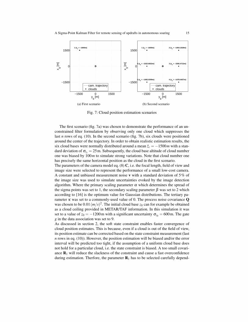
Fig. 7: Cloud position estimation scenarios

The first scenario (fig. 7a) was chosen to demonstrate the performance of an un-constrained filter formulation by observing only one cloud which suppresses thelast n rows of eq. (10). In the second scenario (fig. 7b), six clouds were positionedaround the center of the trajectory. In order to obtain realistic estimation results, thesix cloud bases were normally distributed around a mean zc =−1500m with a stan-dard deviation of σzc = 25m. Subsequently, the cloud base altitude of cloud numberone was biased by 100m to simulate strong variations. Note that cloud number onehas precisely the same horizontal position as the cloud in the first scenario.The parameters of the camera model eq. (8) C, i.e. the focal length, field of view andimage size were selected to represent the performance of a small low-cost camera.A constant and unbiased measurement noise v with a standard deviation of 5% ofthe image size was used to simulate uncertainties evoked by the image detectionalgorithm. Where the primary scaling parameter α which determines the spread ofthe sigma points was set to 1, the secondary scaling parameter β was set to 2 whichaccording to [16] is the optimum value for Gaussian distributions. The tertiary pa-rameter κ was set to a commonly-used value of 0. The process noise covariance Qwas chosen to be 0.01(m/s)2. The initial cloud base z0 can for example be obtainedas a cloud ceiling provided in METAR/TAF information. In this simulation it wasset to a value of z0 =−1200m with a significant uncertainty σz0 = 600m. The gateg in the data association was set to 9.As discussed in section 2, the soft state constraint enables faster convergence ofcloud position estimates. This is because, even if a cloud is out of the field of view,its position estimate can be corrected based on the state constraint measurement (lastn rows in eq. (10)). However, the position estimation will be biased and/or the errorinterval will be predicted too tight, if the assumption of a uniform cloud base doesnot hold for a particular cloud, i.e. the state constraint is biased. A too small covari-ance R1 will reduce the slackness of the constraint and cause a fast overconfidenceduring estimation. Therfore, the parameter R1 has to be selected carefully depend-


ing on cloud base variations that can be encountered in the real world. That beingsaid, R1 was tuned with the second scenario such that the filter ensures estimationconfidence for clouds with an altitude variation of up to 100m. This value roughlycorresponds to the maximum the main author has observed during various cross-country soaring flights and has been confirmed by a meteorologist. The procedurelead to a parameter value of R1 = 750000m2.

4.2 Estimation performance

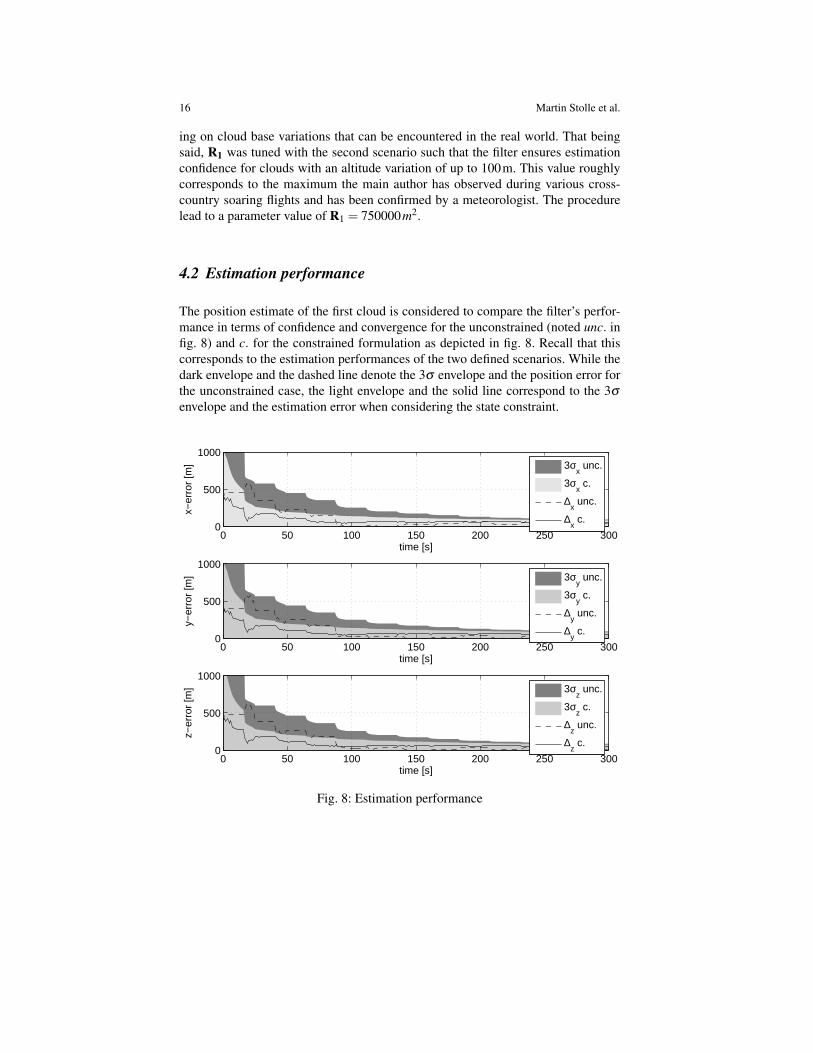
The position estimate of the first cloud is considered to compare the filter’s perfor-mance in terms of confidence and convergence for the unconstrained (noted unc. infig. 8) and c. for the constrained formulation as depicted in fig. 8. Recall that thiscorresponds to the estimation performances of the two defined scenarios. While thedark envelope and the dashed line denote the 3σ envelope and the position error forthe unconstrained case, the light envelope and the solid line correspond to the 3σ

envelope and the estimation error when considering the state constraint.

time [s]

x−er

ror

[m]

0 50 100 150 200 250 3000

500

10003σ

x unc.

3σx c.

∆x unc.

∆x c.

time [s]

y−er

ror

[m]

0 50 100 150 200 250 3000

500

10003σ

y unc.

3σy c.

∆y unc.

∆y c.

time [s]

z−er

ror

[m]

0 50 100 150 200 250 3000

500

10003σ

z unc.

3σz c.

∆z unc.

∆z c.

Fig. 8: Estimation performance


As expected, both regarding rate of convergence and the error, the SCSPKF out-performs the standard SPKF. In all three cases, the upper bound of the position erroris reliably predicted. The huge uncertainty of the initial cloud base impacts the fil-ter’s transient behavior which can be seen in terms of estimation overshoots in thebeginning of the estimation process. Also, the settling time for the unconstrainedfilter process is extended since each cloud is visible only for approximately 35%of the estimation duration. Periods with no measurements can be seen at the longhorizontal segments within the graph. In contrast, for the constrained formulation asignificant reduction of the state’s settling time is obtained due to the measurementaugmentation.Estimation degradation is expected whenever the vertical position of a cloud stronglyvaries from the mean and its position update is only performed using augmentedmeasurements. This is particularly the case for clouds that lie behind the camera’sfield of view when flying towards the next waypoint in cross-country soaring. How-ever, this degradation is not predominant, since clouds that lie behind the vehiclehave no impact on the future path.

5 Perspectives

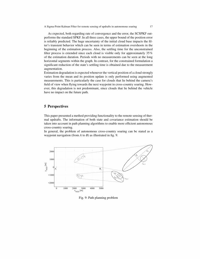
This paper presented a method providing functionality to the remote sensing of ther-mal updrafts. The information of both state and covariance estimation should betaken into account in path planning algorithms to enable more efficient autonomouscross-country soaring.In general, the problem of autonomous cross-country soaring can be stated as awaypoint navigation (from A to B) as illustrated in fig. 9.

0 1000 2000 3000 4000 5000

2000

1000

0

1000

2000

A B

xNED

[m]

yNED[m]

Fig. 9: Path planning problem


In this example, an unpowered UAV glider has to fly from waypoint A to way-point B given position estimates for the two thermal updrafts T1 and T2, where thetrue thermal centers are supposed to lie somewhere within the 2D error ellipses ofthe estimates. The mission starts at waypoint A where the UAV is scanning the skyfor thermals while climbing in a thermal before planning the path to the next in-termediate or global target B. The ability of the glider to perform this mission inminimum time depends on three factors. Firstly, the vehicle’s performance in termsof its glide ratio i.e. its capacity to transform potential energy into travelled dis-tance. Secondly, the flight control’s performance to center around a given thermal.Thirdly and most importantly meteorological conditions and the pilot’s capacity toread them i.e. to locate far away thermals in order to plan the most efficient path.If the direct path from A to B is not feasible due to the vehicle’s limited glide ratio,it has to fly a detour via one of the two thermals to regain altitude. The total flighttime for the two path options is given by

(A→ T1→ B) : tAB = tAT1 + ten,T1 + tth,T1︸︷︷︸time spent at T1

+tT1B

(A→ T2→ B) : tAB = tAT2 + ten,T2 + tth,T2︸︷︷︸time spent at T2

+tT2B

(30)

where the encounter time ten is the time to hit the thermal while searching within theerror ellipse, and the thermal time tth is the time spent in the thermal updraft dur-ing climb. The latter depends on the initial altitude at which the vehicle enters thethermal and the strength of the updraft as well as the cloud base. The vehicle is sup-posed to leave the thermal once the cloud base is reached. Assuming equal thermalstrength, the two routes seem to be on par regarding the flight time. However, thelarger position uncertainty of T1 might require more time to encounter the thermalusing some search pattern whose size is determined by the error ellipse. That beingsaid, the uncertainty of the thermal position impacts the flight time. According toAllen’s research on modeling thermal updrafts for autonomous UAV soaring [4],the thermal radius rth as illustrated in fig. 9 can be predicted when knowing zc andthe altitude z at which the vehicle reaches the thermal

rth = 0.5[

0.203(zzc)

13 (1−0.25

zzc)zc

](31)

Whenever the thermal radius rth is larger than the half of the semi minor b belong-ing to the 2D error ellipse (see T1 in fig. 9), the maximum time to encounter thethermal can be predicted by the speed V (which is considered to be constant duringoperation) and the semi major a

ten =aV

(32)

Otherwise, a systematic search pattern has to be flown within the error ellipse. Re-gardless of the pattern’s shape, the maximum time to encounter the thermal is


ten =lp

Vwhere lp = lp(PT , p) (33)

where the pattern length lp depends on the uncertainty PT as well as on the shape ofthe pattern p.These upper bounds on te render it possible to incorporate the uncertainty of thermalposition estimates into the cost function thus reducing the total flight time.Future work will concentrate on two fields. First, the design of path planning al-gorithms for autonomous cross-country soaring including crucial meteorologicalaspects as thermal updrafts and wind. Second, the design of image processing algo-rithms capable of deducing information about thermals given images of clouds. Thisincludes for instance thermal strength prediction based on the color and contrast ofthe related cumulus as well as cloud size and shape. If those visible features canbe detected, and thermal strength can fairly be predicted, even more efficient pathplanning becomes possible by taking into account this additional information.

6 Conclusion

In this paper, a SCSPKF was developed for remotely sensing thermal updrafts indi-cated by cumulus clouds in autonomous soaring. Two design efforts were focusedon:

• Including the state constraint of a uniform cumulus cloud base for faster conver-gence

• Maintaining estimation consistency and providing a confident estimate of theuncertainty

Simulation results clearly demonstrate the benefits of the constrained filter formula-tion in terms of convergence rate. The filter still provides consistent estimation forstrong model deviations with biases in the cumulus cloud base of up to 100m.Finally, a perspective for a new path planning approach for autonomous cross-country soaring was presented considering the uncertainty of thermal position esti-mates to augment the efficiency of future UAV operations.

References

[1] M. J. Allen and V. Lin, “Guidance and Control of an Autonomous SoaringUAV with Flight TTest Results,” in 45th AIAA Aerospace Sciences and Meet-ing and Exhibit, American Institute for Aeronautics and Astronautics (AIAA),January 2007.

[2] K. Andersson, I. Kaminer, V. Dobrokhodov, and V. Cichella, “Thermal Center-ing Control for Autonomous Soaring; Stability Analysis and Flight Test Re-


sults,” Journal of Guidance Navigation and Control, vol. 35, pp. 963–975,2012.

[3] Naseem Akhtar and James F Whidborne and Alastair K Cooke, “Real-timetrajectory generation technique for dynamic soaring UAVs,” in Proceedings ofthe UKACC International Conference on Control, 2008.

[4] M. J. Allen, “Updraft model for development of autonomous soaring unin-habited air vehicles,” in 44th AIAA Aerospace Sciences Meeting and Exhibit,American Institute for Aeronautics and Astronautics (AIAA), January 2006.

[5] D. J. Edwards and L. M. Silberberg, “Autonomous Soaring: The MontagueCross-Country Challenge,” Journal of Aircraft, vol. 47, pp. 1763–1769, 2010.

[6] N. Kahveci, Robust Adaptive Control For Unmanned Aerial Vehicles. PhDthesis, University of Southern California - Faculty of the Graduate School,USA, 2007.

[7] John Canny, “A Computational Approach to Edge Detection,” IEEE Transac-tions on Pattern Analysis and Machine Intelligence, vol. PAMI-8, pp. 679–698,November 1986.

[8] E. Kleinschmidt, Handbuch der Meteorologischen Instrumente und ihrerAuswertung. Verlag von Julius Springer, 1935.

[9] Dennis Pagen, Understanding the sky. Dennis Pagen, February 1992.[10] T. K. Yaakov Bar-Shalom, X. Rong Li, Estimation with Applications To Track-

ing and Navigation. John Wiley and Sons, Inc., 2001.[11] S. S. Ponda, “Trajectory Optimization for Target Localization Using Small

Unmanned Aerial Vehicles,” Master’s thesis, Massachusetts Institute of Tech-nology, September 2008.

[12] S. Julier, “A skewed approach to filtering,” in In SPIE Conference on Signaland Data Processing of Small Targets, vol. 3373, pp. 271–282, SPIE, April1998.

[13] S. J. Julier and J. K. Uhlman, “A New Extension of the Kalman Filter to Non-linear systems,” in Proc. SPIE 3068, Signal Processing, Sensor Fusion, andTarget Recognition VI, April 1997.

[14] R. V. der Merwe, “The square-root unscented Kalman filter for state and pa-rameter estimation,” in Acoustics, Speech, and Signal Processing, 2001. Pro-ceedings. (ICASSP ’01). 2001 IEEE, vol. 6, pp. 3461–3464, May 2001.

[15] R. V. der Merwe and E. Wan, “The unscented Kalman filter for nonlinear es-timation,” in Adaptive Systems for Signal Processing, Communications, andControl Symposium 2000. AS-SPCC. The IEEE 2000, pp. 153–185, IEEE, Oc-tober 2000.

[16] M. Rhudy and Y. Gu, “Understanding Nonlinear Kalman Filters, Fart II: AnImplementation Guide,” Interactive Robotics Letters, 2013.

[17] J. W. Langelaan, State estimation for autonomous flight in cluttered environ-ments. PhD thesis, Stanford University, March 2006.

[18] M. Montemerlo and S. Thrun, FastSLAM: A Scalable Method For The Simu-lations Localization and Mapping Problem in Robotics. Springer, 2007.

Documents

A Sigma-Point Kalman Filter for remote sensing of updrafts ... · PDF fileA Sigma-Point Kalman Filter for remote sensing of updrafts in ... a certain decay and rebirth ... for remote