A Simple Algorithm for Complete MotionPlanning of Translating Polyhedral Robots

Gokul Varadhan1, Shankar Krishnan2, T.V.N. Sriram3, and DineshManocha4

1 University of North Carolina at Chapel Hill varadhan@cs.unc.edu2 AT&T Labs - Research krishnas@research.att.com3 University of North Carolina at Chapel Hill tvn@cs.unc.edu4 University of North Carolina at Chapel Hill dm@cs.unc.edu

http://gamma.cs.unc.edu/motion

Summary. We present an algorithm for complete path planning for translatingpolyhedral robots in 3D. Instead of exactly computing an explicit representation ofthe free space, we compute a roadmap that captures its connectivity. This repre-sentation encodes the complete connectivity of free space and allows us to performexact path planning. We construct the roadmap by computing deterministic sam-ples in free space that lie on an adaptive volumetric grid. Our algorithm is simpleto implement and uses two tests: a complex cell test and a star-shaped test. Thesetests can be efficiently performed on polyhedral objects using max-norm distancecomputation and linear programming. The complexity of our algorithm varies as afunction of the size of narrow passages in the configuration space. We demonstratethe performance of our algorithm on environments with very small narrow passagesor no collision-free paths.

1 IntroductionPath planning is an important problem in algorithmic robotics. The basicproblem is to find a collision-free path for a robot among rigid objects and ithas been well-studied for over three decades. Some of the earlier interest was indeveloping algorithms for complete path planning. An algorithm is complete,if it is guaranteed to find a solution when one exists and to return failure oth-erwise. It is well known that any complete planner will run in exponential timein the number of degrees-of-freedom (dofs) of the robot [13]. Most practicalalgorithms for complete path planning are restricted to 2D polygonal objectsor 3D convex polytopes or special objects e.g. ladders, discs or spheres.

Given the complexity of a complete path planner, most of the effort inthe last two decades has been on development of approximate approachesincluding those based on cell decomposition and potential field [13]. Theseapproaches can be resolution complete if the resolution parameters are se-lected properly, but not exact or complete. Other algorithms are based onprobabilistic roadmaps [11], which have been successfully applied to manyhigh-dof robots. However, they may not terminate in a deterministic mannerwhen there is no collision-free path.

2 Varadhan et. al.

In this paper, we restrict ourselves to complete path planning for a 3D poly-hedral robot undergoing translation motion among 3D polyhedral obstacles.The configuration space of the robot can be computed based on Minkowskisum of the robot and the obstacles. The Minkowski sum of two convex poly-topes (with n features) can have O(n2) combinatorial complexity and is rel-atively simple to compute. On the other hand, the Minkowski sum of non-convex polyhedra can have complexity as high as O(n6). A commonly usedapproach to compute Minkowski sums decomposes the two non-convex poly-hedra into convex pieces, computes their pairwise Minkowski sums and finallythe union of the pairwise Minkowski sums. The main bottleneck in implement-ing such an algorithm is computing the union of pairwise Minkowski sums.Given m polyhedra, their union can have combinatorial complexity O(m3) andm can be high in the context of Minkowksi sum computation. Furthermore,robust computation of the boundary of the union and handling all degenera-cies remains a major open issue. As a result, no good algorithms are knownfor robust computation of exact Minkowski sum of 3D polyhedral models andcomplete path planning.Main Contributions: We present a novel algorithm for complete path plan-ning for translating polyhedral robots in 3D. We perform convex decompo-sition and compute pairwise Minkowski sums of resulting convex polytopes.Instead of exactly computing the union of these polytopes, we compute a con-nectivity roadmap that captures the connectivity of the free space. We gener-ate the connectivity roadmap by taking deterministic samples on an adaptivevolumetric grid. We employ two main tests during sample generation: com-plex cell test and star-shaped test. These tests can be efficiently performedfor polyhedral objects using max-norm computation and linear programming.The complexity of our algorithm varies as a function of the size of narrowpassages in the configuration space.

Our algorithm is simple to implement in practice. We highlight its perfor-mance on two environments with few hundred polygons with either very smallnarrow passages or no collision-free paths. In these configurations, our algo-rithm takes a few seconds to either compute a collision-free path or guaranteesthat no path exists.Organization: The rest of the paper is organized in the following manner. Wegive a background on motion planning in Section 2 and briefly survey relatedwork. Section 3 gives an overview of our approach. We describe connectivityroadmaps in Section 4 and present an algorithm to compute the roadmap inSection 5. We highlights its performance on some environments in Section6. In Section 7, we give an analysis of our approach and discuss few of itslimitations. We conclude in Section 8.

2 Background and Prior WorkIn this section, we define the general motion planning problem. Let R be arobot consisting of a collection of rigid subparts moving in a Euclidean spaceW , called workspace, represented as Rd, with d = 2 or 3. Let O1, . . . ,Oq

Complete Motion Planning with Translation Motion 3

be fixed rigid objects, hereafter referred as obstacles embedded in W . Assumethat the geometry of R,O1, . . . ,Oq is accurately known, and that there are nokinematic constraints to limit the motion of R. The position and orientationof the subparts define the placement of R (also referred to as a configurationof R). The set of all placements of R defines a configuration space C. Themotion planning problem is defined as: given an initial and goal placementof R, generate a path ρ specifying a continuous sequence of placements of Ravoiding contact with the Oi’s, starting at initial placement and terminatingat the goal placement. Report failure if no such path exist. Every obstacleOi, i = 1, . . . , q, in W maps to the region

COi = {Z ∈ C : R(Z) ∩ Oi 6= φ},in C, where R(Z) is the subset of W occupied by R at the placement Z. Theunion of all COi,

⋃qi=1 COi is called C-obstacle region or forbidden region. The

free configuration space is defined as the set

F = C \q⋃

i=1

COi.

A free path between two free configurations Zinit and Zgoal is a continuousmap ρ : [0, 1]→ F , ρ(0) = Zinit and ρ(1) = Zgoal.2.1 Previous WorkMotion planning has been extensively studied in the literature for more thanthree decades. In this section, we limit our discussion to algorithms for ex-act motion planning or to polyhedral objects undergoing translation motionin 3D. At a broad level they can be classified into the following techniques:roadmaps, cell decomposition, and specialized algorithms for 2D and 3D ob-jects. A comprehensive survey of motion planning results is presented in [13].RoadmapsThe idea underlying this approach is to convert the path planning prob-lem in k-dimensional configuration space to path planning in network of 1-dimensional curves maintaining the connectivity in the robot’s free space. Thevarious types of roadmaps proposed to achieve this task are visibility graph,Voronoi diagram or retraction approach, and silhouettes.

Visibility graph method [13] reduces the problem of motion planning to agraph search. Using this approach, Lozano-Perez and Wesley [15] proposed anO(n3) algorithm which was improved to O(n2 log n) by Lee [14] and to O(n2)by Guibas and Hershberger [9]. An output sensitive algorithm of O(k+n log n),where k is output size, was proposed by Ghosh and Mount [7]. In practice, thistechnique is mostly used for motion planning in two dimensional configurationspaces.

The retraction approach uses the concept of retraction in topology bydefining a continuous mapping of the robot’s free space F onto one-dimensionalnetwork of curves lying in F . When C = R2 and the robot and obstacles arepolygonal, the Voronoi diagram is a roadmap obtained by retraction [21]. Thisapproach provides the additional property that the obtained paths maximizethe clearance between the robot and the obstacles.

4 Varadhan et. al.

Silhouette method was proposed by Canny [4]. Unlike approaches surveyedearlier, this method does not make any assumptions about the configurationspace and is a complete path planning algorithm that runs in single exponen-tial time in the configuration space dimension.Cell DecompositionThese methods are most extensively applied for motion planning problem [13].The crux of this approach is to partition the robot’s free space into a collectionof non-overlapping cells and to construct a connectivity graph representing thecell adjacency. One of the first exact cell decomposition methods for solvingthe general motion planning problem was by Schwartz and Sharir [17].Motion Planning Algorithms for 2D and 3D RobotsDifferent exact algorithms have been proposed for complete motion planningof 2D and 3D robots. Many of them are based on computing the Minkowskidifference and the exact representation of C-obstacle region [15]. Kedem andSharir [12] presented an efficient algorithm for a polygonal robot among polyg-onal obstacles with 3-dof configuration space. A similar algorithm for polyg-onal objects was also developed by Avnaim and Boissonant [3]. Sacks [16]presented a practical configuration space computation algorithm for pairs ofcurved planar parts. Halperin [10] presented efficient and robust algorithmsto compute the Minkowski sum of 2D polygonal objects and used them for ex-act motion of planning of 2D objects undergoing translation motion. Aronovand Sharir [1] present a randomized algorithm to plan the motion of a con-vex polyhedron translating in 3-space amidst convex polyhedral obstacles.Vleugels and Overmars [21] presented a spatial subdivision algorithm to ap-proximate the Voronoi diagram of an environment with convex primitives andused it for motion planning using retraction.

3 OverviewIn this section, we formulate the problem of computing a collision free pathfor a polyhedral object undergoing translation motion in 3D using Minkowskisums, and provide an overview of our approach.3.1 Motion Planning of Translating RobotIn this paper, our focus is on complete motion planning of translating poly-hedral robots in the presence of polyhedral obstacles. It is well known thatfor a translating robot R and an obstacle O, the C-obstacle CO = O⊕ (−R),where ⊕ is the Minkowski sum and −R is R reflected about the origin. Thisformulation shrinks the robot to a point object, and the obstacles Ois aretransformed to the respective Minkowski sums COi.3.2 Minkowski SumThe Minkowski sum of two subsets P and Q of an affine space is definedas P ⊕Q= {x| x = p + q,p ∈ P,q ∈ Q}. It is relatively easier to com-pute Minkowski sums of convex polytopes as compared to general polyhedralmodels. For convex polytopes in 3D, the Minkowski sum can be computed inO(n log n + k) time, where k is the total number of features of the Minkowski

Complete Motion Planning with Translation Motion 5

sums [8]. In the worst case, k = O(n2). However, for non-convex polyhedra in3D, the Minkowski sum can have O(n6) worst-case complexity [5].

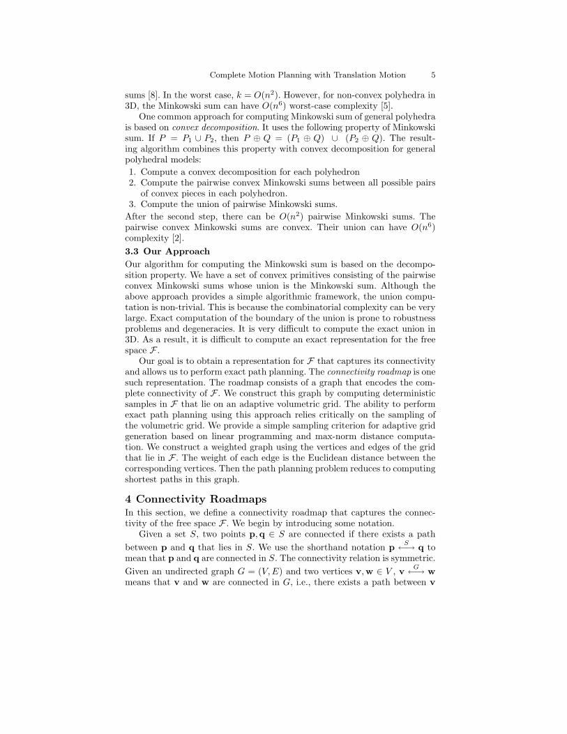
One common approach for computing Minkowski sum of general polyhedrais based on convex decomposition. It uses the following property of Minkowskisum. If P = P1 ∪ P2, then P ⊕ Q = (P1 ⊕ Q) ∪ (P2 ⊕ Q). The result-ing algorithm combines this property with convex decomposition for generalpolyhedral models:1. Compute a convex decomposition for each polyhedron2. Compute the pairwise convex Minkowski sums between all possible pairs

of convex pieces in each polyhedron.3. Compute the union of pairwise Minkowski sums.

After the second step, there can be O(n2) pairwise Minkowski sums. Thepairwise convex Minkowski sums are convex. Their union can have O(n6)complexity [2].3.3 Our ApproachOur algorithm for computing the Minkowski sum is based on the decompo-sition property. We have a set of convex primitives consisting of the pairwiseconvex Minkowski sums whose union is the Minkowski sum. Although theabove approach provides a simple algorithmic framework, the union compu-tation is non-trivial. This is because the combinatorial complexity can be verylarge. Exact computation of the boundary of the union is prone to robustnessproblems and degeneracies. It is very difficult to compute the exact union in3D. As a result, it is difficult to compute an exact representation for the freespace F .

Our goal is to obtain a representation for F that captures its connectivityand allows us to perform exact path planning. The connectivity roadmap is onesuch representation. The roadmap consists of a graph that encodes the com-plete connectivity of F . We construct this graph by computing deterministicsamples in F that lie on an adaptive volumetric grid. The ability to performexact path planning using this approach relies critically on the sampling ofthe volumetric grid. We provide a simple sampling criterion for adaptive gridgeneration based on linear programming and max-norm distance computa-tion. We construct a weighted graph using the vertices and edges of the gridthat lie in F . The weight of each edge is the Euclidean distance between thecorresponding vertices. Then the path planning problem reduces to computingshortest paths in this graph.

4 Connectivity RoadmapsIn this section, we define a connectivity roadmap that captures the connec-tivity of the free space F . We begin by introducing some notation.

Given a set S, two points p,q ∈ S are connected if there exists a pathbetween p and q that lies in S. We use the shorthand notation p S←→ q tomean that p and q are connected in S. The connectivity relation is symmetric.Given an undirected graph G = (V,E) and two vertices v,w ∈ V , v G←→ wmeans that v and w are connected in G, i.e., there exists a path between v

6 Varadhan et. al.

Fig. 1. Connectivity Roadmap: We construct a connectivity roadmap by generat-ing an adaptive voxel grid. The roadmap consists of a connectivity graph which isobtained by considering the set of grid points and grid edges that lie in free space(shown in green in the left figure). Connectivity roadmap also consists of a transferfunction τ that maps points in free space to a vertex in the connectivity graph. Asshown in the right figure, the source p and destination q get mapped to verticesτ(p) and τ(q) respectively. The problem of path planning between p and q reducesto simple graph search between τ(p) and τ(q) in the connectivity graph.

and w consisting of a sequence of edges in E. As before, F refers to the freespace. ∂F denotes the boundary of F . The sign of a point is positive if it liesin F , negative otherwise.

A connectivity roadmap consists of a connectivity graph G.

Definition 1. The connectivity graph G = (V,E,w) is a weighted undirectedgraph defined by a set V of points in free space, a set E of line segments infree space that connect pairs of points in V , and a weight function w : E → R.V and E correspond to the set of vertices and edges of G, respectively.

Definition 2. A transfer function τ : F → V is a mapping such that

∀p ∈ F , p F←→ τ(p)

The connectivity graph satisfies the following two properties:

• Property 1. It encapsulates the connectivity of the free space. Everypoint p ∈ F is connected to atleast one vertex in the connectivity graph.This implies that there exists a transfer function τ that maps a point infree space to a vertex in the connectivity graph. There also exists a transferpath function Γ such that Γ (p) returns the path between p and τ(p) inF .

• Property 2. It captures the connectivity of free space. Two points p,q ∈F are connected in F if and only if the two vertices τ(p), τ(q) ∈ V areconnected in G, i.e.,

p F←→ q ⇐⇒ τ(p) G←→ τ(q)

Definition 3. The connectivity roadmap is defined as the tuple (G, τ, Γ )

Complete Motion Planning with Translation Motion 7

Fig. 1 shows an example of a connectivity roadmap. By combining theabove two properties, we see that the connectivity roadmap satisfies the fol-lowing property:

p F←→ q ⇐⇒ p F←→ τ(p) τ(p) G←→ τ(q) τ(q) F←→ q

This property enables us to perform complete path planning. As long asthe source and destination are connected, we can find a path between themusing the connectivity roadmap. Suppose we wish to find a path between twopoints p,q ∈ F . Assume they are connected. We compute a mapping on theconnectivity graph using the transfer function τ . The transfer path functionΓ gives us the path between p and τ(p), and q and τ(q). Moreover, thereexists a path between τ(p) and τ(q) in the connectivity graph. This path canbe found easily by performing a simple graph search. Call this path γ. Thuswe obtain the path Γ (p) :: γ :: Γ (q) between p and q, where :: denotes a pathconcatenation. In this manner, the connectivity roadmap reduces the problemof path planning to computing a graph shortest path between τ(p) and τ(q).

The above property also provides us with a test for non-existence of apath. If no path exists between p and q in F , we can detect this by testing ifτ(p) and τ(q) are disconnected in G (by Property 2).

5 Connectivity Roadmap ConstructionIn this section, we describe our algorithm to compute the connectivityroadmap.5.1 SamplingWe construct a roadmap by performing a sampling of the free space. Unlikeprevious approaches such as probabilistic roadmaps (PRMs) that generatesamples randomly [11], we construct a roadmap in a deterministic fashion.Our goal is to sample the free space sufficiently to capture its connectivity. Ifwe do not sample the free space adequately, we may not detect valid pathsthat pass through the narrow passages in the configuration space.

In our prior work [20], we proposed a sampling algorithm to generate anoctree grid for the purpose of topology preserving surface extraction. We usethis sampling algorithm to capture the connectivity of free space. We providea brief description of the octree generation algorithm. We refer the reader to[20] for a detailed description. The algorithm starts with a single grid cellthat is large enough to capture relevant features of F . It performs two tests,complex cell test and star-shaped test, to decide whether to subdivide a gridcell.Complex Cell TestA cell is complex if it has a complex voxel, face, edge, or an ambiguous signconfiguration. We define a voxel (face) of a grid cell to be complex if it inter-sects ∂F and the grid vertices belonging to the voxel (face) do not exhibit asign change (see Figs. 2(a) & 2(b)). The sign of a vertex is positive if it lieswithin F , negative otherwise. An edge of the grid cell is said to be complex if∂F intersects the edge more than once (see Fig. 2(c)).

8 Varadhan et. al.

Fig. 2. This figure shows the different cases corresponding to the complex cell andstar-shaped test. Figs (a), (b), (c) and (d) show cases of complex voxel, complexface, complex edge, and ambiguous sign configuration. The white and black circlesdenote positive and negative grid points respectively. Fig. (e) shows the case wherethe surface is not star-shaped w.r.t a voxel. In Fig (f), the restriction of the surfaceto the right face of the cell is not star-shaped.

There are two types of sign ambiguities — face ambiguity and voxel am-biguity [22]. When the signs at the vertices of a single face alternate duringcounterclockwise (or clockwise) traversal, the resulting configuration is a faceambiguity. A voxel ambiguity results when any pair of diagonally opposite ver-tices have one sign while the other vertices have a different sign (see Fig. 2(d)).Either of these cases is defined as an ambiguous sign configuration. We classifygrid cells with such sign configurations as complex.

Intuitively, the complex cell criterion ensures that the surface intersectsthe grid cell in a simple manner in most cases. We use max-norm distancecomputation to perform the complex cell test [20]. Max-norm distance is usedto determine whether ∂F intersects a voxel/face/edge of the cell. It can becomputed efficiently for polyhedral primitives. If a grid cell is complex, it issubdivided and the algorithm is recursively applied to each of its children.Star-shaped TestLet S be a nonempty subset of Rn. The set Kernel(S) consists of all s ∈ Ssuch that for any x ∈ S, we have s+λ(x− s) ∈ S,∀λ ∈ [0, 1]. S is star-shapedif Kernel(S) 6= ∅. We refer to a point belonging to Kernel(S) as an origin ofS. A star-shaped primitive has at least one representative point (origin) suchthat all the points in the primitive are visible from it.F is defined to be star-shaped with respect to (w.r.t) a voxel v if Fv = F∩v

is star-shaped. Similarly, F is defined to be star-shaped w.r.t a face f if thetwo-dimensional set, Ff = F ∩ f , is star-shaped. F is said to be star-shapedw.r.t a cell if it is star-shaped w.r.t the cell’s voxel, and each of its six faces.If F is not star-shaped w.r.t the cell (see Figs. 2(e) & 2(f)), then the cell issubdivided and the algorithm is recursively applied to the children cells.

We use linear programming to perform the star-shaped test [20]. By def-inition, a polyhedron is star-shaped if it has a non-empty kernel. If p is apoint belonging to the kernel, then each face of the polyhedron with centroidc and outward normal n defines the linear constraint n · (c − p) > 0 on p.As a result, the kernel is non-empty if the set of constraints admits a feasiblesolution for p.

The star-shaped and complex cell tests can be performed very efficiently.Moreover, performing these tests does not require an explicit representationof F . It works even when the surface is represented as a Boolean combination

Complete Motion Planning with Translation Motion 9

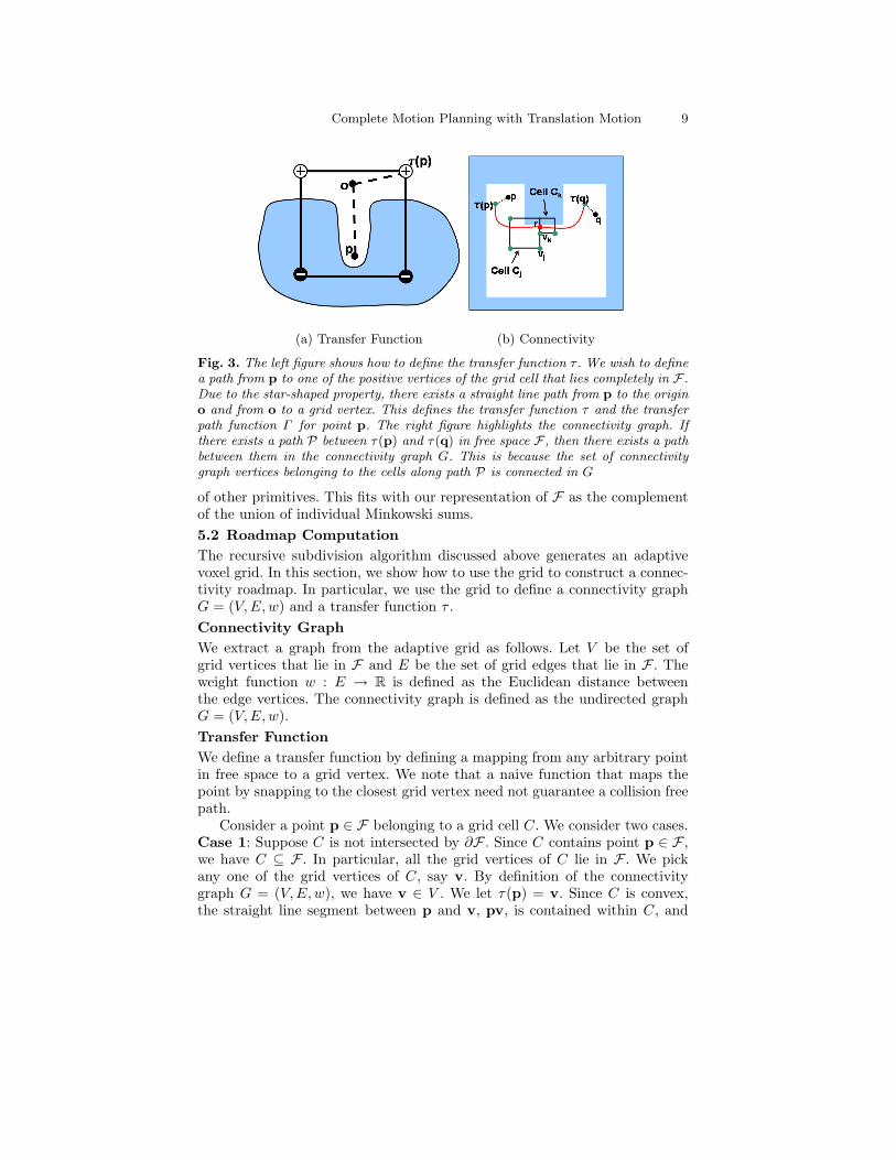
(a) Transfer Function (b) Connectivity

Fig. 3. The left figure shows how to define the transfer function τ . We wish to definea path from p to one of the positive vertices of the grid cell that lies completely in F .Due to the star-shaped property, there exists a straight line path from p to the origino and from o to a grid vertex. This defines the transfer function τ and the transferpath function Γ for point p. The right figure highlights the connectivity graph. Ifthere exists a path P between τ(p) and τ(q) in free space F , then there exists a pathbetween them in the connectivity graph G. This is because the set of connectivitygraph vertices belonging to the cells along path P is connected in G

of other primitives. This fits with our representation of F as the complementof the union of individual Minkowski sums.5.2 Roadmap ComputationThe recursive subdivision algorithm discussed above generates an adaptivevoxel grid. In this section, we show how to use the grid to construct a connec-tivity roadmap. In particular, we use the grid to define a connectivity graphG = (V,E, w) and a transfer function τ .Connectivity GraphWe extract a graph from the adaptive grid as follows. Let V be the set ofgrid vertices that lie in F and E be the set of grid edges that lie in F . Theweight function w : E → R is defined as the Euclidean distance betweenthe edge vertices. The connectivity graph is defined as the undirected graphG = (V,E, w).Transfer FunctionWe define a transfer function by defining a mapping from any arbitrary pointin free space to a grid vertex. We note that a naive function that maps thepoint by snapping to the closest grid vertex need not guarantee a collision freepath.

Consider a point p ∈ F belonging to a grid cell C. We consider two cases.Case 1: Suppose C is not intersected by ∂F . Since C contains point p ∈ F ,we have C ⊆ F . In particular, all the grid vertices of C lie in F . We pickany one of the grid vertices of C, say v. By definition of the connectivitygraph G = (V,E,w), we have v ∈ V . We let τ(p) = v. Since C is convex,the straight line segment between p and v, pv, is contained within C, and

10 Varadhan et. al.

therefore lies within F . Therefore, the transfer function satisfies the propertyp F←→ τ(p). Further, the transfer path function Γ (p) = pv.Case 2: Consider the case where C is intersected by ∂F . Due to the star-shaped property, FC = F ∩ C is star-shaped. Let o be the origin of FC .Because the cell is not complex, there exists at least one grid vertex in FC .Let this vertex be v. We let τ(p) = v. Due to the star-shaped property, bothv and p are “visible” from o. Since the line segments po and ov lie in F , wehave p F←→ τ(p) (see Fig. 3(a)). This also gives us the transfer path function,Γ (p) = po :: ov.5.3 Connectivity GuaranteeIn this section, we show that the connectivity roadmap defined above capturesthe connectivity of F . This is formally expressed in Theorem 1. We begin bypresenting a lemma. Given a cell C, the connectivity graph restricted to C isgiven by GC = (VC , EC) where VC and EC denote the set of grid points andgrid edges respectively of cell C that lie in F . We have dropped the weightfunction from the graph notation for convenience. It is assumed to be theEuclidean distance function.

Lemma 1. Given a cell C, the graph GC = (VC , EC) is connected.Proof: Consider any two grid vertices v,w ∈ VC . We prove that v GC←→ w. Itsuffices to prove that there exists a sequence of grid cell edges connecting vand w that do not intersect F . We consider three cases:

• Case 1: The grid points v and w are the endpoints of an edge of thecell. Since both v and w have the same (positive) sign and the edge is notcomplex, this edge cannot intersect ∂F . Therefore the edge belongs to EC

and we have v GC←→ w.• Case 2: The grid vertices v and w lie diagonally opposite on a cell face.

The case where the other two grid vertices on the face are negative cor-responds to a case of face ambiguity. Therefore, at least one of the othertwo grid vertices (say u) on the face has a positive sign. v and u are twopositive grid vertices on the endpoints of an edge of the cell. Thereforeby Case 1, we have v GC←→ u. Similarly, we have u GC←→ w. This impliesv GC←→ w.

• Case 3: The grid points v and w are diagonally opposite vertices of thecell. The case where all the other grid vertices are negative correspondsto a case of voxel ambiguity. Therefore, at least one other grid vertex uhas a positive sign. Depending on u’s position, the vertices v and u eitherreduce to Case 1 or 2 (u and w will belong to the other case). Therefore,v GC←→ u and u GC←→ w which implies v GC←→ w.

2Since GC is a subgraph induced by G, any two vertices v, w ∈ VC satisfyv G←→ w.

Theorem 1.p F←→ q ⇐⇒ τ(p) G←→ τ(q)

Complete Motion Planning with Translation Motion 11

Proof: We first prove that if τ(p) G←→ τ(q), then we have p F←→ q. Byconstruction of the transfer function, we have p F←→ τ(p) and q F←→ τ(q).Moreover, because graph G consists of vertices and edges in F , we have

τ(p) G←→ τ(q) =⇒ τ(p) F←→ τ(q)

Therefore, we have p F←→ q.We now prove the converse. Let p F←→ q. We have

τ(p) F←→ p, p F←→ q, q F←→ τ(q)

Therefore, we have τ(p) F←→ τ(q). If τ(p) and τ(q) belong to the same gridcell, then Lemma 1 ensures that τ(p) G←→ τ(q).

Consider the case where τ(p) and τ(q) belong to different cells, Cp andCq respectively. There exists a path between τ(p) and τ(q) in F . Let Ci, i =0, . . . n, be the set of cells that are intersected by this path such that C0 = Cp

and Cn = Cq. Suppose the path passes from a cell Cj into an adjacent cellCk. Let the corresponding connectivity graphs restricted to Cj and Ck beGCj

= (Vj , Ej) and GCk= (Vk, Ek) respectively. According to Lemma 1,

both Vj and Vk are connected in graph G. The path passes from cell Cj to Ck

through a face of the cell. Let fj be the face of Cj that is incident on Ck andfk be the face of Ck that is incident on Cj . Since grid cells Cj and Ck can beat different resolutions, fj and fk need not be identical. The path penetratesfaces fj and fk at a common point r that lies in F (see Fig. 3(b)). Since bothfaces fj and fk are not complex and have at least one point in F , they containpositive vertices vj ∈ Vj and vk ∈ Vk respectively that lie in F . We will show

below that vjG←→ vk. As a result, Vj ∪ Vk is connected in graph G. This is

true of all the cells along the path. Therefore, τ(p) and τ(q) are connected ingraph G and we have τ(p) G←→ τ(q).

We now return to the proof of the result vjG←→ vk. The octree subdivision

ensures that one of the faces fj and fk is a subset of the other. Let f denotethe larger of the two faces. Vertices vj and vk lie on f . Using the facts thatf is not complex and that F is star-shaped w.r.t f , it can be shown that theset Ff = F ∩ f is connected [20]. This implies that vertices vj and vk are

connected in Ff , i.e., vjFf←→ vk. We wish to prove that vj

G←→ vk.This is a two-dimensional version of the above theorem. Since our con-

straints of complex cell and star-shapedness extend to all the faces and edgesof the cell, we can apply our argument recursively. The base case of our re-cursion is the one-dimensional case where we need to show that two points onan edge connected in F are also connected through G. This is readily shownby observing that the edges of the grid cells are not complex.

2

12 Varadhan et. al.

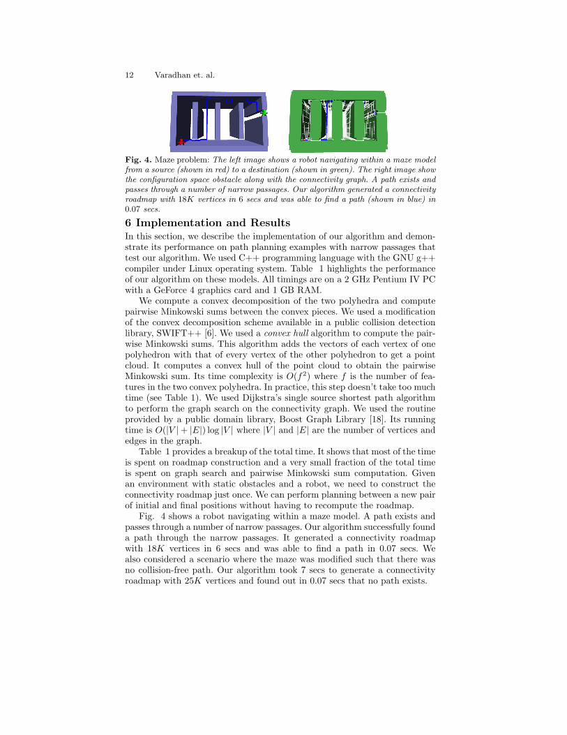
Fig. 4. Maze problem: The left image shows a robot navigating within a maze modelfrom a source (shown in red) to a destination (shown in green). The right image showthe configuration space obstacle along with the connectivity graph. A path exists andpasses through a number of narrow passages. Our algorithm generated a connectivityroadmap with 18K vertices in 6 secs and was able to find a path (shown in blue) in0.07 secs.

6 Implementation and ResultsIn this section, we describe the implementation of our algorithm and demon-strate its performance on path planning examples with narrow passages thattest our algorithm. We used C++ programming language with the GNU g++compiler under Linux operating system. Table 1 highlights the performanceof our algorithm on these models. All timings are on a 2 GHz Pentium IV PCwith a GeForce 4 graphics card and 1 GB RAM.

We compute a convex decomposition of the two polyhedra and computepairwise Minkowski sums between the convex pieces. We used a modificationof the convex decomposition scheme available in a public collision detectionlibrary, SWIFT++ [6]. We used a convex hull algorithm to compute the pair-wise Minkowski sums. This algorithm adds the vectors of each vertex of onepolyhedron with that of every vertex of the other polyhedron to get a pointcloud. It computes a convex hull of the point cloud to obtain the pairwiseMinkowski sum. Its time complexity is O(f2) where f is the number of fea-tures in the two convex polyhedra. In practice, this step doesn’t take too muchtime (see Table 1). We used Dijkstra’s single source shortest path algorithmto perform the graph search on the connectivity graph. We used the routineprovided by a public domain library, Boost Graph Library [18]. Its runningtime is O(|V |+ |E|) log |V | where |V | and |E| are the number of vertices andedges in the graph.

Table 1 provides a breakup of the total time. It shows that most of the timeis spent on roadmap construction and a very small fraction of the total timeis spent on graph search and pairwise Minkowski sum computation. Givenan environment with static obstacles and a robot, we need to construct theconnectivity roadmap just once. We can perform planning between a new pairof initial and final positions without having to recompute the roadmap.

Fig. 4 shows a robot navigating within a maze model. A path exists andpasses through a number of narrow passages. Our algorithm successfully founda path through the narrow passages. It generated a connectivity roadmapwith 18K vertices in 6 secs and was able to find a path in 0.07 secs. Wealso considered a scenario where the maze was modified such that there wasno collision-free path. Our algorithm took 7 secs to generate a connectivityroadmap with 25K vertices and found out in 0.07 secs that no path exists.

Complete Motion Planning with Translation Motion 13

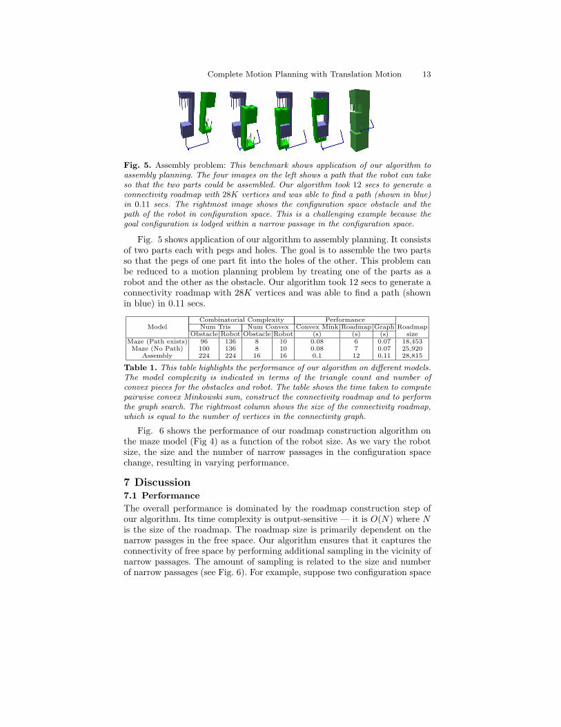
Fig. 5. Assembly problem: This benchmark shows application of our algorithm toassembly planning. The four images on the left shows a path that the robot can takeso that the two parts could be assembled. Our algorithm took 12 secs to generate aconnectivity roadmap with 28K vertices and was able to find a path (shown in blue)in 0.11 secs. The rightmost image shows the configuration space obstacle and thepath of the robot in configuration space. This is a challenging example because thegoal configuration is lodged within a narrow passage in the configuration space.

Fig. 5 shows application of our algorithm to assembly planning. It consistsof two parts each with pegs and holes. The goal is to assemble the two partsso that the pegs of one part fit into the holes of the other. This problem canbe reduced to a motion planning problem by treating one of the parts as arobot and the other as the obstacle. Our algorithm took 12 secs to generate aconnectivity roadmap with 28K vertices and was able to find a path (shownin blue) in 0.11 secs.

Combinatorial Complexity PerformanceModel Num Tris Num Convex Convex Mink Roadmap Graph Roadmap

Obstacle Robot Obstacle Robot (s) (s) (s) sizeMaze (Path exists) 96 136 8 10 0.08 6 0.07 18,453Maze (No Path) 100 136 8 10 0.08 7 0.07 25,920

Assembly 224 224 16 16 0.1 12 0.11 28,815

Table 1. This table highlights the performance of our algorithm on different models.The model complexity is indicated in terms of the triangle count and number ofconvex pieces for the obstacles and robot. The table shows the time taken to computepairwise convex Minkowski sum, construct the connectivity roadmap and to performthe graph search. The rightmost column shows the size of the connectivity roadmap,which is equal to the number of vertices in the connectivity graph.

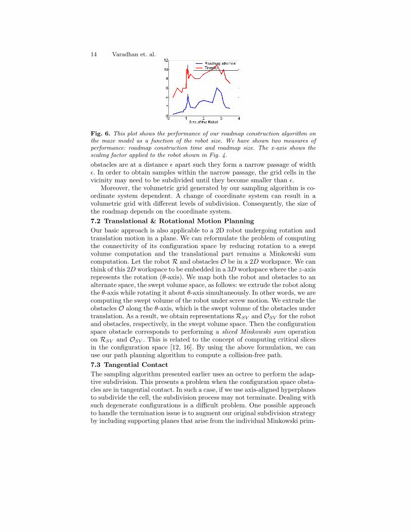
Fig. 6 shows the performance of our roadmap construction algorithm onthe maze model (Fig 4) as a function of the robot size. As we vary the robotsize, the size and the number of narrow passages in the configuration spacechange, resulting in varying performance.

7 Discussion7.1 PerformanceThe overall performance is dominated by the roadmap construction step ofour algorithm. Its time complexity is output-sensitive — it is O(N) where Nis the size of the roadmap. The roadmap size is primarily dependent on thenarrow passges in the free space. Our algorithm ensures that it captures theconnectivity of free space by performing additional sampling in the vicinity ofnarrow passages. The amount of sampling is related to the size and numberof narrow passages (see Fig. 6). For example, suppose two configuration space

14 Varadhan et. al.

Fig. 6. This plot shows the performance of our roadmap construction algorithm onthe maze model as a function of the robot size. We have shown two measures ofperformance: roadmap construction time and roadmap size. The x-axis shows thescaling factor applied to the robot shown in Fig. 4.

obstacles are at a distance ε apart such they form a narrow passage of widthε. In order to obtain samples within the narrow passage, the grid cells in thevicinity may need to be subdivided until they become smaller than ε.

Moreover, the volumetric grid generated by our sampling algorithm is co-ordinate system dependent. A change of coordinate system can result in avolumetric grid with different levels of subdivision. Consequently, the size ofthe roadmap depends on the coordinate system.7.2 Translational & Rotational Motion PlanningOur basic approach is also applicable to a 2D robot undergoing rotation andtranslation motion in a plane. We can reformulate the problem of computingthe connectivity of its configuration space by reducing rotation to a sweptvolume computation and the translational part remains a Minkowski sumcomputation. Let the robot R and obstacles O be in a 2D workspace. We canthink of this 2D workspace to be embedded in a 3D workspace where the z-axisrepresents the rotation (θ-axis). We map both the robot and obstacles to analternate space, the swept volume space, as follows: we extrude the robot alongthe θ-axis while rotating it about θ-axis simultaneously. In other words, we arecomputing the swept volume of the robot under screw motion. We extrude theobstacles O along the θ-axis, which is the swept volume of the obstacles undertranslation. As a result, we obtain representationsRSV and OSV for the robotand obstacles, respectively, in the swept volume space. Then the configurationspace obstacle corresponds to performing a sliced Minkowski sum operationon RSV and OSV . This is related to the concept of computing critical slicesin the configuration space [12, 16]. By using the above formulation, we canuse our path planning algorithm to compute a collision-free path.7.3 Tangential ContactThe sampling algorithm presented earlier uses an octree to perform the adap-tive subdivision. This presents a problem when the configuration space obsta-cles are in tangential contact. In such a case, if we use axis-aligned hyperplanesto subdivide the cell, the subdivision process may not terminate. Dealing withsuch degenerate configurations is a difficult problem. One possible approachto handle the termination issue is to augment our original subdivision strategyby including supporting planes that arise from the individual Minkowski prim-

Complete Motion Planning with Translation Motion 15

itives themselves. This is akin to binary space partitioning (BSP) technique.Cells generated by this approach are no longer cubical, but general convexpolyhedra. It is easy to prove that such a technique will always terminate[19].7.4 LimitationsOur sampling algorithm uses two criteria: complex cell test and star-shapedtest to guide the subdivision. These criteria are conservative. Consequently,our algorithm may perform unnecessary subdivision. This can reduce the per-formance of our algorithm and result in a larger roadmap than necessary. Theconvex decomposition method can result in a large number of convex pieces.Given two polyhedra each with n convex pieces, we obtain n2 pairwise con-vex Minkowski sums. Since this set of pairwise convex Minkowski sums is aninput to our algorithm, its large size affects the performance of the overallalgorithm.

8 Conclusion and Future WorkWe have presented an algorithm for complete path planning for translatingpolyhedral robots in 3D. Our algorithm is based on constructing a connectivityroadmap that captures the connectivity of the free space. It is guaranteed tofind a collision-free path if one exists. Otherwise it detects non-existence ofany collision-free path.

Our algorithm is simple to implement in practice. It uses two tests: a com-plex cell test and a star-shaped test. These tests can be efficiently performedfor polyhedral objects using max-norm distance computation and linear pro-gramming. The complexity of our algorithm varies as a function of the sizeof the narrow passages in configuration space. We highlight the performanceof our algorithm on two environments with very small narrow passages or nocollision-free paths.

There are many avenues for future work. For some applications, a robotis allowed to be in contact with the obstacles. We would like to extend ouralgorithm to accommodate this. We are interested in application of our algo-rithm to the problem of motion planning for a robot with translational androtational degrees of freedom. Finally, we would like to improve the roadmapgeneration algorithm by making our approach less conservative and improvethe overall performance.

9 AcknowledgmentsThis research is supported in part by ARO Contracts DAAD19-02-1-0390 andW911NF-04-1-0088, NSF awards ACI 9876914 and ACR-0118743, ONR Con-tracts N00014-01-1-0067 and N00014-01-1-0496, DARPA Contract N61339-04-C-0043 and Intel. We thank Danny Halperin for many fruitful discussionson the complexity and practical implementations of Minkowski sums in 3D.

References1. B. Aronov and M. Sharir. On translational motion planning in 3-space. In ACM

Symposium on Computational Geometry, pages 21–30, 1994.

16 Varadhan et. al.

2. B. Aronov, M. Sharir, and Boaz Tagansky. The union of convex polyhedra inthree dimensions. SIAM Journal on Computing, 26:1670–1688, 1997.

3. Francis Avnaim and J.-D. Boissonnat. Practical exact motion planning of aclass of robots with three degrees of freedom. In Proc. of Canadian Conferenceon Computational Geometry, page 19, 1989.

4. J.F. Canny. The Complexity of Robot Motion Planning. ACM Doctoral Disser-tation Award. MIT Press, 1988.

5. D. Dobkin, J. Hershberger, D. Kirkpatrick, and S. Suri. Computing theintersection-depth of polyhedra. Algorithmica, 9:518–533, 1993.

6. S. Ehmann and M. C. Lin. Accurate and fast proximity queries between poly-hedra using convex surface decomposition. Computer Graphics Forum (Proc. ofEurographics’2001), 20(3):500–510, 2001.

7. S. K. Ghosh and D. M. Mount. An output sensitive algorithm for computingvisibility graphs. In Proc. 28th Annu. IEEE Sympos. Found. Comput. Sci.,pages 11–19, 1987.

8. L. Guibas and R. Seidel. Computing convolutions by reciprocal search. DiscreteComput. Geom, 2:175–193, 1987.

9. L. J. Guibas and J. Hershberger. Computing the visibility graph of n linesegments in O(n2) time. Bull. EATCS, 26:13–20, 1985.

10. D. Halperin. Robust geometric computing in motion. International Journal ofRobotics Research, 21(3):219–232, 2002.

11. L. Kavraki, P. Svestka, J. C. Latombe, and M. Overmars. Probabilisticroadmaps for path planning in high-dimensional configuration spaces. IEEETrans. Robot. Automat., pages 12(4):566–580, 1996.

12. K. Kedem and M. Sharir. An efficient motion planning algorithm for a con-vex rigid polygonal object in 2-dimensional polygonal space. Discrete Comput.Geom., 5:43–75, 1990.

13. J.C. Latombe. Robot Motion Planning. Kluwer Academic Publishers, 1991.14. D. T. Lee. Proximity and reachability in the plane. Report R-831, Dept. Elect.

Engrg., Univ. Illinois, Urbana, IL, 1978.15. T. Lozano-Perez and M. Wesley. An algorithm for planning collision-free paths

among polyhedral obstacles. Comm. ACM, 22(10):560–570, 1979.16. E. Sacks. Practical sliced configuration space for curved planar pairs. Interna-

tional Journal of Robotics Research, 18(1), 1999.17. J. T. Schwartz and M. Sharir. On the piano movers probelem ii, general tech-

niques for computing topological properties of real algebraic manifolds. Ad-vances of Applied Maths, 4:298–351, 1983.

18. J. G. Siek, L. Lee, and A. Lumsdaine. The Boost Graph Library: User Guideand Reference Manual. Addison-Wesley, Boston, 2002.

19. TVN Sriram, Gokul Varadhan, and Dinesh Manocha. Handling degeneraciesduring adaptive subdivisions. In UNC Technical Report TR04-14, 2004.

20. G. Varadhan, S. Krishnan, T. V. N. Sriram, and D. Manocha. Topology preserv-ing surface extraction using adaptive subdivision. Technical report, Departmentof Computer Science, University of North Carolina, 2004.

21. J. Vleugels and M. Overmars. Approximating Voronoi diagrams of convex sitesin any dimension. International Journal of Computational Geometry and Ap-plications, 8:201–222, 1997.

22. Jane Wilhelms and Allen Van Gelder. Topological considerations in isosurfacegeneration extended abstract. Computer Graphics, 24(5):79–86, 1990.