A simple descriptive method for multidimensional item

A simple descriptive method for multidimensional item

response theory based on stochastic dominance

Georg Schollmeyer Christoph Jansen Thomas Augustin

Abstract

In this paper we develop a descriptive concept of a (partially) ordinal joint scaling ofitems and persons in the context of (dichotomous) item response analysis. The developedmethod has to be understood as a purely descriptive method describing relations amongthe data observed in a given item response data set, it is not intended to directly measuresome presumed underlying latent traits. We establish a hierarchy of pairs of item dicultyand person ability orderings that empirically support each other. The ordering principleswe use for the construction are essentially related to the concept of rst order stochasticdominance. Our method is able to avoid a paradoxical result of multidimensional itemresponse theory models described in Hooker et al. [2009]. We introduce our concepts inthe language of formal concept analysis. This is due to the fact that our method has somesimilarities with formal concept analysis and knowledge space theory: Both our methodsas well as descriptive techniques used in knowledge space theory (concretely, item treeanalysis) could be seen as two dierent stochastic generalizations of formal implicationsfrom formal concept analysis.

Keywords: stochastic dominance, empirically mutually supportive pairs, formal concept analy-sis, knowledge space theory, cognitive diagnosis models, formal implications, item tree analysis

1 Introduction

The fruitful development of psychometric models that are empirically adequate is alwayschallenged by the fact that one has to deal with latent constructs that, without anyquasi metaphysical theory or vague preconceptions of involved terms, lead to a systematicunder-determination of involved concepts. A sound scientic theory that makes all basicterms like that of ability or diculty rigorously empirically criticizable is dicult to obtain.The exact understanding of the latent structure as a truly underlying trait or only as amerely rough sketch or simply only an analogy about what is going on behind the observablescene has a straight impact on how to interpret results of psychometric tests and how to dealwith a seemingly paradoxical situation, rstly described in Hooker et al. [2009]. This paradoxis prevalent in many multidimensional models of item response theory (IRT), includingRasch-type models that are not only statistical models for analyzing item response data, buthave some seemingly solid measurement theoretic foundation that can possibly be shatteredby such a paradox.

The aim of the present paper is to provide a more or less naive descriptive viewpoint onthe problem of obtaining some notion of person ability and item diculty, given one simply

1

has observed, how a set of persons answered a set of items in a psychometric test. Ourdescriptive method avoids the above-mentioned paradox.

The paper is structured as follows: In Section 2 we recall the paradox discovered by Hookeret al. [2009] and give a possible explanation of the paradox. In Section 3 we introduce ourdescriptive method for a relational notion of person ability and item diculty. We describeour ideas in the language of formal concept analysis. The basics of formal concept analysisare briey sketched in Appendix A for the reader unfamiliar with this topic. Actually, forthe understanding of Section 3 it is not really needed to know much about formal conceptanalysis. The reason for presenting our ideas in the language of formal concept analysis isthat it has a neat relation to knowledge space theory (and also to cognitive diagnosis models),which is a nonparametric form of item response theory where the analysis of the paradox isalso of some interest. In Section 4 we analyze the paradox in the context of knowledge spacetheory. A brief introduction to the basics knowledge space theory is also given in Appendix B.Appendix C shortly sketches the relationship between formal context analysis and knowledgespace theory. Section 5 gives a brief data example comparing the herein developed methodwith a descriptive method of item tree analysis and sketches, how our method behaves undercertain unidimensional item response models. Finally, Section 6 concludes.

2 The paradox

We start by explaining the paradox we are referring to:

Jane and Jill are fast friends who are nonetheless intensely competitive.At the end of high school, they each take an entrance exam for a prestigiousuniversity. After the exam, they compare notes and discover that they gave thesame answers for every question but the last. On checking their materials, itis clear that Jane answered this question correctly, but Jill answered incorrectly.They are therefore very surprised, when the test results are published, to nd thatJill passed but Jane did not.

Lawsuits ensue. The university maintains that it followed well-established sta-tistical procedures: The questions on the test were designed to simultaneously ex-amine both language and analytic skills, and a multiple-hurdle rule (Segall, 2000)based on maximum likelihood estimates of each student's abilities was used to en-sure that admitted students were procient in both. The university had recheckedits calculations many times and was satised the correct decision had been made.Jane's lawyers countered that, whatever the statistical correctness of the agency'sprocedures, it is unreasonable that an examinee should be penalized for getting morequestions correct. ([Hooker et al., 2009, p. 419])

Before coming to an explanation and discussion of this paradox we want to emphasize thefact that the paradox is not a marginal note arising in only a few instances of multidimen-sional IRT models and data situations, it can be shown that this sort of paradox can (andto some extent will) arise in broad classes of multidimensional IRT models (cf. Hooker et al.[2009], Jordan and Spiess [2012], Finkelman et al. [2010]), it is also present in some modelsof knowledge space theory (see Section 4). Note further that the paradox does not arise only

2

because of the need to estimate an underlying ability of a person, which is subject to statisticalerror. Also if one would replace the actually observed responses patterns by true underlyingresponse probabilities one could get such a paradox. (Of course, for many usual models, suchparadoxical situations are somehow asymptotically avoided, given the presumed model is ac-tually true, cf., [Jordan, 2013, Section 4.1] and [Hooker et al., 2009, Theorem 8.1]). This isimportant to keep in mind to understand the next considerations. An intuitive explanationwhy the paradox can appear is given in Hooker et al. [2009]:

Suppose that each question on the test given to Jane and Jill required bothlanguage and analytical skills to answer correctly, and Jane and Jill got some ofthese correct and some incorrect. The nal question, however, was very dicultin terms of analysis, but did not require strong language skills. That Jane gotthis question correct suggests that her analytical skills must be very good indeed.This being the case, the only explanation for her previous incorrect answers isthat her language skills must be quite low. By contrast, Jill, in getting the nalquestion incorrect, has demonstrated fewer analytic skills and must have relied onstronger language skills to answer previous questions correctly. The estimate ofJane's language ability therefore dipped below the required threshold, while Jill'swas pushed upward; both obtained satisfactory analysis scores. ([Hooker et al.,2009, p. 420])

The authors of Hooker et al. [2009] conclude that they nonetheless feel that it is better notto put students in the position of second-guessing when their best answer may be harmful tothem ([Hooker et al., 2009, p. 420]), however, there are dierent reactions thinkable. Threeof many possible reactions are:

i) Everything is alright here, because given that the model is true, we have appropriatelyestimated the true abilities of Jill and Jane and thus appropriately decided for Jill becauseof her sucient language skills and against Jane because her language skills were notsucient.

ii) Maybe everything is alright, but at least from the point of view of some notionof fairness (which is a concept independent of the notions of ability and diculty) weshould only use psychometric methods for the approval of students that do not admit thisparadox.

iii) The paradox reveals two very dierent conceptualizations of the term abilitythat should not be confused: On the one hand one can understand the term ability as anunderlying trait that one tries to measure, and thus the responses given in the exam haveto be taken only as measurements that are only indirectly related to the underlying trait.On the other hand one can understand the ability literally as the ability to solve this orthat item and so one has to take the responses not only as measurements but as the actualresults showing exactly which items a persons was able to solve in the concrete test andwhich not. In this understanding, one could alternatively use the word success insteadof the word ability. Then there would be no need in estimating abilities, but a naturallyarising question would then be, which of two persons that solved dierent questions wasmore successful.

3

The rst reaction is problematic in the sense that one cannot assume that the model isexactly right, because a rigorous empirical test of such an IRT model is not really possibledue to the involved latent concepts (see also the discussion in [Michell, 2008b]). Especiallythe dimension of the IRT model plays an important role, here: If we could have (and oneshould have) doubt about the (clearly only very roughly adequate) statement the test itemsonly test the dimensions language skill and analytical skill , then the situation may change:In a very extreme (and of course unrealistic) opposite situation one could assume that in caseof doubt every item tests mainly its own dimension. Then, clearly the paradox should notbe present anymore, because then Jane would be more able w.r.t. every dimension that wastested.

The second reaction is maybe confronted with the objection Why is it unfair to basean approval on honest estimates of abilities and not to revise a decision only because ofthe fact that actually Jane did answer one more question rightly? The fact that Janeanswered one more question rightly is only revealing that she solved the items actually givenin the test better and not that she has more abilities. If one accepts the second reaction,then one could do for example a constrained optimization, like proposed in Hooker et al. [2009].

The third reaction is of interest in this paper, where we take the response patterns at facevalue to dene a descriptive notion of success.

3 A descriptive method based on concepts of stochastic domi-nance

In this section, we develop a purely descriptive and relational notion of person success anditem diculty. We start with a motivating example to introduce our ideas:

3.1 A motivational example

Tim and Danny are companioned pole vaulters. From time to time theydiscuss about the adequacy of the pole vault rules which actually made Dannybetter ranked than Tim in the last three competitions, seemingly only because hewas more smart in skipping the right heights: In 2015 everything was in order,Tim passed the 5.70m in the rst trial and failed the following 5.75m while Dannypassed both heights in the rst trail. In 2016 their dierence was more tight:While both failed the 5.70m for the rst two trials, Tim took the 5.70m in thethird trial but Danny skipped the 5.70m and passed the 5.75m in the rst trial.The height of 5.80m they both did not manage. Finally, in 2017 Danny's luckin skipping heights beggared all description: Again Tim passed the 5.70m in thethird trial and then took all heights till 5.90m in the rst trial until he failed the5.95m. But Danny, also passing the 5.70m in the third trial, decided to skip thefollowing 4 heights and luckily passed the 5.95m in the rst trial.

In discussions between Danny and Tim, Danny usually argues that the rulesare simply the rules and thus skipping heights is of course right if the luck is withyou. But Tim objects:

4

Beside the rules, what would be a reasonable argumentation showing that inthe last three years you were actually the more capable pole vaulter? Dannyinterrupts:If you had force me to also jump the skipped heights between 5.75m and 5.90mthen I would probably have passed it, because I also managed the 5.95m.Tim: Oh, this is wild speculation. But let us make the problem more simple:Assume we both did jump the same heights, say only one time, and you failed allheights from 5.75m to 5.90m while I passed all these heights. Would you still saythat you are the better pole vaulter only because you managed the 5.95m and Inot?Danny: Of course I would say this, 5.95m is an extraordinary performance, nearto the olympic record.Tim: Oh, I doubt that the dierence between 5.90m and 5.95m is so much tomake up for four failed 5.90m′s.Danny: You cannot compare one passed 5.95m with 4 failed heights of 5.90m.

Tim: Of course I cannot compare, but also you cannot compare, so what couldwe do?...

The situation of pole vaulting has some similarities with the situation in item responsetheory, both Tim and Danny are solving items, but there are important dierences, whichmake the analysis more simple, here. Concretely, we have the following two specic points:

i) The items of jumping a specic height have some intrinsic properties that make themtotally ordered in diculty. If one idealizes the situation a little bit, then one can saythat if one is able to take some height c, then one is also able to take a height d that islower than c. To see this, one can argue that for jumping the height d, one can put thebar at height d and jump, as if the bar would lie on height c, and because one is able tojump height d, one would automatically also take height c. It is important to note thatthis relational property between height c and height d is an intrinsic property of theitems jumping height c and jumping height d, which is due to some physical relationbetween the tasks. In particular, it is not dependent upon who is trying to solve thetask, so here we have no dependency of the notion of diculty upon a population. Thisindependence is also the aim in item response theory in Rasch's understanding (specicobjectivity, cf., [Rasch, 1977]), but there it often seems to be more a wish than a fact.

ii) The task of jumping a given height can be repeated by the same person. The repetitionof the trials of one xed person jumping a xed height can be idealized as a binomialexperiment where one repeats a number of Bernoulli trials with some success probabi-lity p. Approximately, the trials can be assumed to be independent, at least if there isenough time for regeneration between dierent trials and if possible learning eects canbe neglected. In typical situations of item response theory, it is not useful to pose thesame question twice to the same person because of the presence of strong learning eects.The fact that the pole vaulting trials can be repeated makes a statement like Tim has aprobability of taking 5.90m of around 0.9 a somehow empirically testable statement1,

1At least if one accepts Poppers methodological decision for a practical falsication, cf., [Popper, 2005,p. 182]

5

while in typical situations of item response theory, one cannot test a comparable state-ment for one person and one item in isolation. One would have to rely on either otheritems, from which one knows (but wherefrom?) that they have the same diculty, or onitems, from which one can somehow translate the probabilities of solving that items tothe probability of solving the envisaged item. For this one needs a model like the Raschmodel that has to be also valid to allow for such a translation. But beforehand one doesnot know that the Rasch model holds. In this sense, in the spirit of the Duheme-Quineproblem one can test one single item and one single person only together with e.g. theRasch model.

3.2 Person ability and item diculty in pole vaulting

So, let us now try to motivate some notion of item diculty and person ability rstly for thesimple situation of pole vaulting. As already said, there is some clear total order between thedierent items of jumping given heights that are due to physical relations. One can ask ifthere is more than an ordinal scale, for example a cardinal scale of measurement underlying,here. The heights itself clearly have a cardinal scale of measurement. But in pole vaulting,one is not interested mainly in the heights itself, but in the question, if one is able to take,or if one actually did take a given height. If one thinks in the probability of taking a givenheight, then it is reasonable to assume that the success probability is decreasing in the height,but there seems to be no obvious specic functional form describing the success probability independence on the height. Actually, the reason for sometimes managing a given height andsometimes not is due to auxiliary conditions that are not genuinely related to the height orthe experiment, but to the not explicitly stated circumstances.

Thus, practically, more than an ordinal scale of measurement seems to be not reachable,here. Of course, in principle, if we exactly know the auxiliary conditions then we possiblycan explicitly determine the quantitative relation between the success probabilities and theheight and other auxiliary conditions. Practically, this seems unrealistic.Compared to the auxiliary conditions that introduced the randomness of sometimes takinga height and sometimes not, in the Rasch model, the randomness in solving an item is nota sort of noise from which one would like to get rid of, instead it is the basic ingredientthat allows for the construction of a cardinal scale of item-diculty. If no randomnesswere present, then strangely enough one would fall back into the situation of Guttmanscaling, where one has only an ordinal scale of measurement. This counterintuitive issue isknown as the Rasch paradox (see, [Michell, 2008a,b], cf., also [Sijtsma, 2012, Humphry, 2013]).

Since we are not concerned with more than a (partially) ordinal scale in this paper, we donot have to care about this issue, here.

To get a notion of ability of Tim and Danny seems to be hard. For the item diculty, wegot only a relational notion of diculty, thus we would also only expect a relational notionfor person ability. We said that some height c with c > d is more dicult than a height of dbecause if one is able to jump the height c, then one is also able to jump the height d. In adual manner one can say that one person p is more able than another person q, if person p isable to take all heights that person q is able to take. Here, we face the rst slight asymmetrybetween person ability and item diculty2. For the items, we have some physical relation

2Note that a further asymmetry consists in the fact that the ability of a person is related to which item one

6

that translates to a relation about the diculty of items. If we could analyze both Tim andDanny as two dierent physical machines then we could possibly get also a notion of whichheights Danny and Tim are physically able to take. This would be ne, but is of course toodicult. A further point is here, that we spoke about the ability to solve an item, but ofcourse we actually meant some notion of being in principle able to take a height, becausesometimes one takes a height and sometimes not. For the comparison of diculty we didnot need to rely on which heights Danny and Tim actually did take. For the comparing ofpersons, it seems to be practically not circumventable to rely on which items the personsactually did solve.

3.3 A notion of item diculty and person success in item response theory

To get a notion of person ability, let us rstly think about the still more simple case whereone has items that are completely comparable, say Danny and Tim did only try to take thesame height c for a number of trials. Then one can naturally say that a person who solvedmore items than another person is more able than the other person. Actually, because of therandomness of solving an item or not, we would like to be a little more cautious here andsay only that the person who solved more items is more successful than the other person.The above notion can be mathematically expressed in dierent ways. One way would be tocalculate the item scores (i.e., the number of solved items) and then to say that the personwith a higher score is more successful. This formulation seems to do not naturally translateto the case where we have items with dierent diculties with an only ordinal scale ofmeasurement. Thus, another representation seems to be promising, here:

For the case of items that are clearly comparable in diculty, one can say that personp is more successful than person q, if for every item i that person q did solve, there existsalso an item Φ(i) that person p did solve, with the additional condition that Φ is injectivemeaning that we use no item from the items that p has solved twice as an argument to showthat person p is more successful than person q. This representation with a sort of a matchingis the main idea in this paper, and this idea is closely related to the notion of stochasticdominance, see Appendix D. Now, we can think about how we would generalize this notionto the case of items with dierent diculties. The generalization is actually very intuitive:For two persons p and q one can naturally dene that person p is more successful than personq if for every item i there (bijectively) exists another item Φ(i) that is as least as dicult asitem i and was solved by person p.

After having found a notion of successfulness for persons if the diculties of items aregiven, we can now think about how to dene a successfulness-relation when there is nodiculty relation given beforehand, which is the typical case in item response theory.

Before doing so, we would rstly like to point out that there are still very interestingsituations, in which one has at least a partial ordering of item diculty beforehand thatis due to an understanding of the cognitive processes that are needed to solve an item. Aclassical example are fraction subtraction tasks in the context of cognitive diagnosis models

considers (e.g. pole vaulting or climbing or whatever) whereas the diculty of an item is more intrinsicallyrelated to the item and not so much to the question about who tried to solve it.

7

(CDM: Bolt [2007], de la Torre [2009], DiBello and Stout [2007], Junker and Sijtsma [2001],Tatsuoka [1990, 2002]). If one compares for example solving the subtraction task 6/7 − 4/7with the task 2− 1/3, then one can say that the rst task is easier than the second, becausefor solving the rst task one has essentially only to subtract the nominators, while forthe second task, one has to rstly convert the 2 to 6/3 and then one has to subtract thenominators. Thus, everyone who can solve the second task usually is also able to solve therst task, and in this sense the rst task is easier, which is a relation inherent in the tasksand not related to the person who solves the task. Apart from cognitive diagnosis models,also in knowledge space theory ([Doignon and Falmagne, 1985, 2012, Falmagne et al., 1990,Falmagne and Doignon, 2010]) one similarly has some relations between dierent items.Actually, there is a neat relation between the two areas which seemingly independentlydeveloped very similar concepts. While in knowledge space theory one rstly had a moredeterministic view that was generalized to probabilistic versions afterwards (e.g., the basiclocal independence model.), in cognitive diagnosis modeling one came more from classicalitem response theory with a clear probabilistic underpinning and had the aim of bringingitem response theory closer to cognitive psychology. For a detailed discussion of the linkbetween cognitive diagnosis models and knowledge space theory, see Heller et al. [2015].Note further, that both knowledge space theory and cognitive diagnosis models are somehowrelated to the theory of formal concept analysis, see Rusch and Wille [1996]. This relationis the reason for presenting our ideas in terms of formal concept analysis. (Actually, forthe understanding of the ideas developed herein, one does not need to know much aboutformal concept analysis, basically one only needs to know, what a formal context is andwhat a formal implication is, see Appendix A). The paradox described in Hooker et al.[2009] was given in the context of more classical multidimensional IRT models, but onecan also ask for the presence of the paradox in the context of knowledge space theory (orcognitive diagnosis models). This question will thus be also discussed in Section 4 of this paper.

Coming back to the problem of dening a successfulness relation in a general IRT situationwhere one has neither some physical insights into person abilities nor a relation on theitem diculties, at rst glance it seems to be impossible to get a reasonable successfulnessrelation. However, in a rst step, one can try to solve the problem of a missing itemdiculty relation by thinking about a dual construction that could lead to a reasonablediculty relation in a situation where one has knowledge about the abilities of the per-sons. The following notion of item diculty, given a notion person ability seems to be natural:

For two items i and j and for a set of persons with the same ability who all tried to solveitem i and item j one can say that item i is more dicult than item j if there are less personswho solved item i than persons who solved item j. Equivalently, one can say that item i ismore dicult than item j if for every person p who solved item i there bijectively exists aperson Ψ(p) who solved item j. For persons with dierent abilities, one can say that item iis more dicult than item j if for every person p who solved item i there bijectively exists aperson Ψ(p) who is not more able than person p and solved item j.

Now, of course one does not know beforehand the abilities of the persons and one is thusrunning in circles. However, this running in circles can be made from a necessity to a virtue bysimultaneously treating item diculty and person success relations. A diculty relation indu-ces a successfulness relation and vice versa, so one can think about pairs of relations that t

8

to each other. This is the idea behind the notion of empirically mutually supportive pairs thatwe would like to introduce more formally in the following section. The notion of empiricallymutually supportive pairs will be closely related to the notion of rst order stochastic domi-nance, see Appendix D. Since there are more equivalent denitions of stochastic dominance,we also give two equivalent and intuitively accessible denitions of associated success and ea-siness relations in Denition 1 which prepares the notion of empirically mutually supportivepairs given in Denition 2.

3.4 Empirically mutually supportive pairs

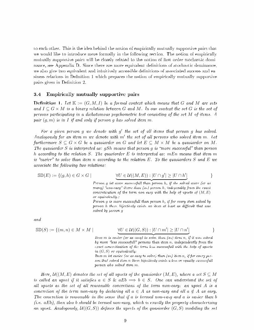
Denition 1. Let K := (G,M, I) be a formal context which means that G and M are setsand I ⊆ G×M is a binary relation between G and M . In our context the set G is the set ofpersons participating in a dichotomous psychometric test consisting of the set M of items. Apair (g,m) is in I if and only if person g has solved item m.

For a given person g we denote with g′ the set of all items that person g has solved.Analogously for an item m we denote with m′ the set of all persons who solved item m. Letfurthermore S ⊆ G × G be a quasiorder on G and let E ⊆ M ×M be a quasiorder on M .The quasiorder S is interpreted as: gSh means that person g is more successful than personh according to the relation S. The quasiorder E is interpreted as: mEn means that item mis easier to solve than item n according to the relation E. To the quasiorders S and E weassociate the following two relations:

SD(E) := (g, h) ∈ G×G | ∀U ∈ U((M,E)) : |U ∩ g′| ≥ |U ∩ h′|︸︷︷︸Person g ist more successfull than person h, if she solved more (or asmany) non-easy items than (as) person h, independtly from the exactconcretization of the term non-easy with the help of upsets of (M,E)or equivalently.:Person g is more successfull than person h, if for every item solved byperson h there bijectively exists an item at least as dicult that wassolved by person g

and

SD(S) := (m,n) ∈M ×M | ∀U ∈ U((G,S)) : |U ∩m′| ≥ |U ∩ n′|︸︷︷︸Item m is easier (or as easy) to solve than (as) item n, if it was solvedby more less successfull persons than item n, independently from theexact concretization of the term less successfull with the help of upsetsin (G,S) or equivalently:Item m ist easier (or as easy to solve) than (as) item n, if for every per-son that solved item n there bijectively exists a less or equally successfullperson who solved item m.

Here, U((M,E) denotes the set of all upsets of the quasiorder (M,E), where a set S ⊆Mis called an upset if it satises a ∈ S & aEb =⇒ b ∈ S. One can understand the set ofall upsets as the set of all reasonable concretions of the term non-easy: an upset A is aconcretion of the term non-easy by declaring all a ∈ A as non-easy and all a /∈ A as easy.The concretion is reasonable in the sense that if a is termed non-easy and a is easier than b(i.e. aEb), then also b should be termed non-easy, which is exactly the property characterizingan upset. Analogously, U((G,S)) denes the upsets of the quasiorder (G,S) modeling the set

9

of all reasonable concretions of the term non-successful.

Now, dene additionally the space S := (S,E) | S ∈ 2G×G, E ∈ 2M×M and endow Swith the order

≤S:= ((S,E), (S′, E′)) ∈ S×S | S ⊆ S′& E ⊆ E′,

and nally dene the operator

L : (S,≤S) −→ (S,≤S) : (S,E) 7→ L((S,E)) := (SD(E) ∩ S, SD(S) ∩ E).

Denition 2. Let K := (G,M, I) be a formal context and (S,E) ∈ S a pair of a person- andan item-quasiorder. The pair (S,E) is called a weakly empirically mutually supportive

pair of K, ifS ⊆ SD(E) & E ⊆ SD(S)

or equivalently(S,E) = L((S,E))

holds. If we actually haveS = SD(E) & E = SD(S),

then the pair (S,E) is called a strongly empirically mutually supportive pair of K. Theset of all weakly empirically mutually supportive pairs of K is denoted with wsupp(K) and theset of all strongly empirically mutually supportive pairs of K is denoted with ssupp(K) .

We can interpret a given weakly empirically mutually supportive pair (S,E) as follows:If we would have some reason to believe that E is the truly underlying easiness relation ofthe items, then the relation S would be a reasonable relation that is somehow empiricallysupported by the easiness relation E. Dually, if we have some reasons to think that S is thetruly underlying success relation, then E would be empirically supported by S as a reasonableeasiness relation. So,we can think of mutually supportive pairs as possible underlying pairsof relations that are consistent in the sense that they support each other. There are much ofthese pairs and one can think about the structure of these pairs. It will turn out that thereis a weakest and a strongest such pair. More importantly, one can explicitly compute theseboth extreme pairs. Furthermore, in some sense, all empirically mutually supportive pairswill avoid the paradox of Hooker et al. [2009] in the sense that a person, who solved all itemsanother person solved, plus some more, is always more successful w.r.t. the relation S thanthe other person. Actually, the weakest mutually supportive pair (S,E) exactly given by

pSq ⇐⇒ person p solved all items that where solved by person q

andiEj ⇐⇒ item i was solved by all persons that solved item j.

The still more interesting pair is the strongest pair that could be seen as the strongestrelational notion of diculty and success one could expect to get, only based on the data. Tosee, that there actually exists such a strongest pair and to see how to compute it, we onlyhave to analyze, what happens if we apply the operator L several times.

Lemma 1 (Lemma and Denition). Let K = (G,M, I) be a nite formal context (meaningthat G and M , and thus also I are nite). The operator L has the following properties:

10

i) it is monotone: ∀p, q ∈ S : p ≤S q =⇒ L(p) ≤S .L(q)

ii) L is intensive: ∀p ∈ S : L(p) ≤S p.

iii) L is of nite order: ∃k ∈ N : Lk+1 := L L . . . L︸︷︷︸k+1 times

= Lk.

iv) If we dene L∞ as Lk with the k from iii), then L∞ is a kernel operator, that is, amonotone, intensive and idempotent operator, where idempotent means that L2

∞ = L∞.

Proposition 1. Let K = (G,M, I) be a nite formal context.

i) The set wsupp(K) of all weakly empirically mutually supportive pairs of K are exactly thekernels of the kernel operator L∞. (This means that p ∈ wsupp(K) ⇐⇒ L∞(p) = p).

ii) The set ssupp(K) of all strongly empirically mutually supportive pairs of K is a subset ofS that has a smallest and a greatest element.

The smallest element (I∂G,1(K), I∂M,1(K)) of this interval consists of the dual relation ofthe simple formal implications between objects

I∂G,1(K) := (h, g) ∈ G×G | ∀m ∈M : gIm =⇒ hIm.

and of the dual relation of the simple formal implications between attributes

I∂M,1(K) := (n,m) ∈M ×M | ∀g ∈ G : gIm =⇒ gIn.

The greatest element is given as

L∞((G×G,M ×M))

or equivalently asL∞((#G,#M )),

where #G := (g, h) | |g′| ≥ |h′| and #M := (m,n) | |m′| ≥ |n′|.

4 Relation to knowledge space theory and formal concept ana-lysis

The reason for introducing our ideas in the language of formal concept analysis lies inthe fact that the weakest empirically mutually supportive pair is build by simple formalimplications and that the construction of success-relations from easiness-relations and viceversa can be seen as some stochastic generalization of simple implications based on ideas ofstochastic dominance. In knowledge space theory, which in its deterministic form is closelyrelated to formal concept analysis (see [Rusch and Wille, 1996] and Appendix C), for theconstruction of the knowledge structure one sometimes uses techniques of Boolean analysis,for example item tree analysis (cf., e.g., [Schrepp, 1999, 2002, Ünlü and Sargin, 2010]). Thisdescriptive technique can be also seen as some other type of a generalization of simple formalimplications:If in an IRT data set, all persons, who solved item i did also solve item j, then the formal im-plication i −→ j is valid and one would naturally say that item j seems to be more easy than

11

item i. For our stochastic generalization, if for simplicity all persons have the same ability, wewould also say that item j is more easy than item i if only more persons solved item j thanitem i, no matter, which persons exactly solved the items. Another generalization of the for-mal implication i −→ j would be to say that item j is more easy than item i if the implicationi −→ j is not exactly true but approximately in the sense that from the population of personswho solved item i most persons (say more than c · 100% of this population) did also solveitem j. This notion, which is very close to the notion of statistical preference3 ([De Schuy-mer et al., 2003b,a]), is one of the underlying ideas in descriptive methods of item tree analysis.

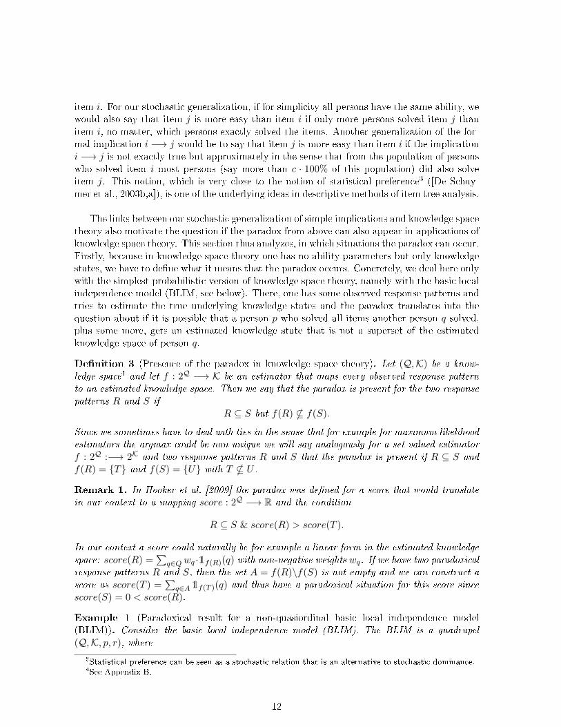
The links between our stochastic generalization of simple implications and knowledge spacetheory also motivate the question if the paradox from above can also appear in applications ofknowledge space theory. This section thus analyzes, in which situations the paradox can occur.Firstly, because in knowledge space theory one has no ability parameters but only knowledgestates, we have to dene what it means that the paradox occurs. Concretely, we deal here onlywith the simplest probabilistic version of knowledge space theory, namely with the basic localindependence model (BLIM, see below). There, one has some observed response patterns andtries to estimate the true underlying knowledge states and the paradox translates into thequestion about if it is possible that a person p who solved all items another person q solved,plus some more, gets an estimated knowledge state that is not a superset of the estimatedknowledge space of person q.

Denition 3 (Presence of the paradox in knowledge space theory). Let (Q,K) be a know-ledge space4 and let f : 2Q −→ K be an estimator that maps every observed response patternto an estimated knowledge space. Then we say that the paradox is present for the two responsepatterns R and S if

R ⊆ S but f(R) * f(S).

Since we sometimes have to deal with ties in the sense that for example for maximum likelihoodestimators the argmax could be non-unique we will say analogously for a set-valued estimatorf : 2Q :−→ 2K and two response patterns R and S that the paradox is present if R ⊆ S andf(R) = T and f(S) = U with T * U .

Remark 1. In Hooker et al. [2009] the paradox was dened for a score that would translatein our context to a mapping score : 2Q −→ R and the condition

R ⊆ S & score(R) > score(T ).

In our context a score could naturally be for example a linear form in the estimated knowledgespace: score(R) =

∑q∈Qwq ·1f(R)(q) with non-negative weights wq. If we have two paradoxical

response patterns R and S, then the set A = f(R)\f(S) is not empty and we can construct ascore as score(T ) =

∑q∈A 1f(T )(q) and thus have a paradoxical situation for this score since

score(S) = 0 < score(R).

Example 1 (Paradoxical result for a non-quasiordinal basic local independence model(BLIM)). Consider the basic local independence model (BLIM). The BLIM is a quadrupel(Q,K, p, r), where

3Statistical preference can be seen as a stochastic relation that is an alternative to stochastic dominance.4See Appendix B.

12

i) (Q,K) is a knowledge space with nite Q,

ii) p is a probability function on K, meaning that p : K −→ [0, 1] with∑

K∈Kp(K) = 1,

iii) r is a response function for (Q,K, p), meaning that r : 2Q × K −→ [0, 1] with∑R∈2Q

r(R,K) = 1 for arbitrary K ∈ K,

iv) r satises the condition of local independence:

r(R,K) =∏

q∈K\R

βq ·∏

q∈K∩R(1− βq) ·

∏q∈R\K

ηq ·∏

q∈Q\(R∪K)

(1− ηq).

Here the βq are the probabilities of a careless error and the ηq are the probabilities of alucky guess for each item q.

Now, take the underlying knowledge space (Q,K) as Q = qq, . . . , q5 and K = ∅,K :=q1, q2, q4, L := q1, q2, q3, q5, Q. Note that K is closed under arbitrary unions but notunder arbitrary intersections because K ∩L = q1, q2 /∈ K, thus (Q,K) is not a quasi-ordinalknowledge space. Furthermore assume that the careless error and the lucky-guess probabilitiesare known and equal for all q. Thus we will denote them with β and η respectively andassume that 0 < η < β < 0.5 which implies in particular that (1 − η) > (1 − β) > 0.5 and(1−x)

x > 1 for x ∈ β, η as well as β(1 − β) > η(1 − η). (These inequalities will be usedlater.) Finally, take for simplicity for p the uniform distribution on all knowledge statesK ∈ K. For a given observed response pattern R the maximum likelihood estimator for the un-derlying true knowledge space is simply that k in K that maximizes the response value r(R,K).

We are now ready to construct a pair of paradoxical response patterns, namely R :=q1, q2 and S := q1, q2, q3, q5. The following calculations will show that the maximumlikelihood estimate of response pattern R is L and the maximum likelihood estimate of S is K,but L * K

q1 q2 q3 q4 q5

Q x x x x xK x x x xL x x x∅R x xS x x x x

13

r(R,L) = β1 · (1− β)2 · η0 · (1− η)2 r(S,K) = β0 · (1− β)4 · η0 · (1− η)1

r(R,Q) = β3 · (1− β)2 · η0 · (1− η)0 r(S,Q) = β1 · (1− β)4 · η0 · (1− η)0

r(R,K) = β2 · (1− β)2 · η0 · (1− η)1 r(S,L) = β1 · (1− β)2 · η2 · (1− η)0

r(R, ∅) = β0 · (1− β)0 · η2 · (1− η)3 r(S, ∅) = β0 · (1− β)0 · η4 · (1− η)1

r(R,L)

r(R,Q) =(1− η)2

β2=

(1− ηη

)2

> 1r(S,K)

r(S,Q) =(1− η)β

> 1

r(R,L)

r(R,K)=

(1− η)β

> 1r(S,K)

r(S,L)=

(1− β)2(1− η)βη2

=(1− β)β

· (1− β)η

· (1− η)η

> 1

r(R,L)

r(R, ∅) =(1− η)β

> 1r(S,K)

r(S,L)=

(1− β)2(1− η)βη2

=(1− β)β

· (1− β)η

· (1− η)η

> 1

r(R,L)

∅ =β(1− β)2

η2(1− η) =β(1− β)η(1− η) ·

(1− β)η

> 1r(S,K)

r(S, ∅) =(1− β)4

η4=

(1− βη

)4

> 1

The following theorem shows that the paradox cannot occur if we have a xed quasi-ordinalknowledge space with known probabilities βq and ηq.

Theorem 1. Let (Q,K, p, r) be a basic local independence model where the underlying know-ledge space is a quasi-ordinal knowledge space and where the careless-error and the lucky-guessprobabilities are known and lie in the interval (0, 0.5). Then, the conditioned maximum likeli-hood estimator5

f : 2Q −→ K : R 7→ f(R) := argmaxK∈K r(R,K)

is not susceptible to the paradox, meaning that there are no two response patterns R and Swith a unique ML estimate f(R) and f(S) satisfying

R ⊆ S & f(R) * f(S).

Proof. Let R and S be two arbitrary response patterns with R ⊆ S andwith unique ML-estimates satisfying f(R) * f(S). We will rstly denesome associated sets and illustrate the situation by a small cross tab andsketch the basic idea of the proof before actually doing the proof: Dene:

5conditioned means here that one maximizes not the unconditional joint likelihood P(R = r & S = K)where R is the random response pattern, r is the actually observed response pattern and S is the randomtrue knowledge state, but one only maximizes P(R = r | S = K) which is equivalent to maximizing the jointlikelihood under the assumption that all knowledge spaces are equally probable.

14

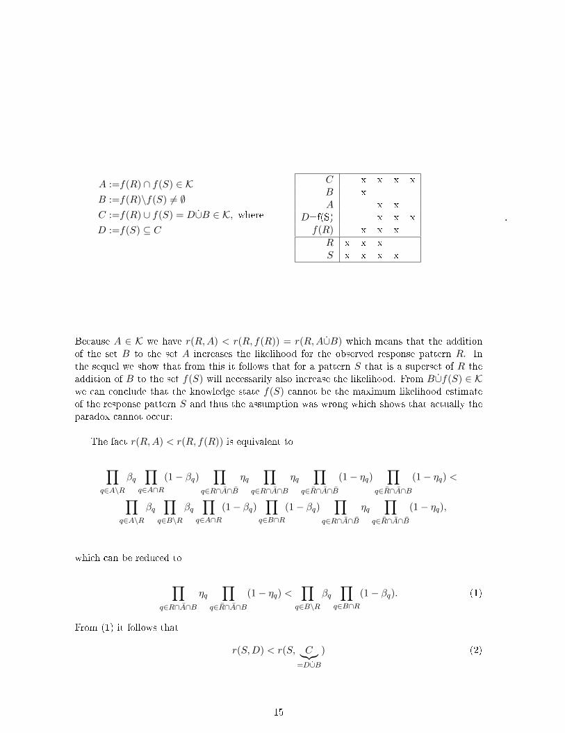
A :=f(R) ∩ f(S) ∈ KB :=f(R)\f(S) 6= ∅C :=f(R) ∪ f(S) = D∪B ∈ K, whereD :=f(S) ⊆ C

C x x x xB xA x x

D=f(S) x x xf(R) x x x

R x x xS x x x x

.

Because A ∈ K we have r(R,A) < r(R, f(R)) = r(R,A∪B) which means that the additionof the set B to the set A increases the likelihood for the observed response pattern R. Inthe sequel we show that from this it follows that for a pattern S that is a superset of R theaddition of B to the set f(S) will necessarily also increase the likelihood. From B∪f(S) ∈ Kwe can conclude that the knowledge state f(S) cannot be the maximum likelihood estimateof the response pattern S and thus the assumption was wrong which shows that actually theparadox cannot occur:

The fact r(R,A) < r(R, f(R)) is equivalent to

∏q∈A\R

βq∏

q∈A∩R(1− βq)

∏q∈R∩A∩B

ηq∏

q∈R∩A∩B

ηq∏

q∈R∩A∩B

(1− ηq)∏

q∈R∩A∩B

(1− ηq) <

∏q∈A\R

βq∏

q∈B\R

βq∏

q∈A∩R(1− βq)

∏q∈B∩R

(1− βq)∏

q∈R∩A∩B

ηq∏

q∈R∩A∩B

(1− ηq),

which can be reduced to

∏q∈R∩A∩B

ηq∏

q∈R∩A∩B

(1− ηq) <∏

q∈B\R

βq∏

q∈B∩R(1− βq). (1)

From (1) it follows that

r(S,D) < r(S, C︸︷︷︸=D∪B

) (2)

15

because (2) is equivalent to∏q∈D\S

βq∏

q∈D∩S(1− βq)

∏q∈S∩D∩B

ηq∏

q∈S∩D∩B

ηq∏

q∈S∩D∩B

(1− ηq)∏

q∈S∩D∩B

(1− ηq) <

∏q∈D\S

βq∏

q∈B\S

βq∏

q∈D∩S(1− βq)

∏q∈B∩S

(1− βq)∏

q∈S∩D∩B

ηq∏

q∈S∩D∩B

ηq,

which can be reduced to∏q∈S∩D∩B

ηq∏

q∈S∩D∩B

(1− ηq) <∏

q∈B\S

βq∏

q∈B∩S(1− βq). (3)

To see that (3) follows from (1) rst note that D ∩ B = A ∩ B = B and remember that S isa superset of R. Then we can derive (3) from (1) as

∏q∈S∩D∩B

ηq∏

q∈S∩D∩B

(1− ηq) <∏

q∈R∩A∩B

ηq∏

q∈R∩A∩B

(1− ηq)

<∏

q∈B\R

βq∏

q∈B∩R(1− βq)

<∏

q∈B\S

βq∏

q∈B∩S(1− βq),

where the rst and the third inequality can be recognized by observing that we have a productof terms greater than 0.5 (the terms (1− βq) and (1− ηq)) and terms less than 0.5 (the termsβq and ηq) and in the product of the left hand sides of the inequalities we have always a subsetof terms greater than 0.5 and a superset of terms less than 0.5 compared to the correspondingright hand sights. The second inequality is the inequality from (1).

16

Remark 2. Note that the theorem assumes that the careless error and lucky guess parametersare known. If they are estimated jointly for all response patterns under the assumption thatthey are identical for every person (which is actually assumed in the BLIM), then the paradoxstill cannot occur. If, on the other hand, one estimates the lucky guess and careless errorprobabilities for each person separately, then the paradox can occur. This is shown in thefollowing example:

Example 2. Assume the BLIM with the modication that the careless error probabilitiesand the lucky guess probabilities are independent from the items but that they are estimatedseparately for every person via (conditioned) maximum likelihood. The conditioned likelihoodfor a given response pattern R, an underlying true knowledge state K and careless error- andlucky guess probabilities β and η is given as

β|K\R| · (1− β)|K∩R| · η|R\R| · (1− η)|R∪K|.

Assuming β, η ∈ [0, 5], the likelihood is maximal if

βML(R,K) =

min0.5, |K\R|

|K\R|+|K∩R| if |K\R|+ |K ∩R| 6= 0

∈ [0, 0.5] if |K\R|+ |K ∩R| = 0(4)

ηML(R,K) =

min0.5, |R\K|

|R\K|+|K∪R| if |R\K|+ |K ∪R| 6= 0

∈ [0, 0.5] if |R\K|+ |K ∪R| = 0.

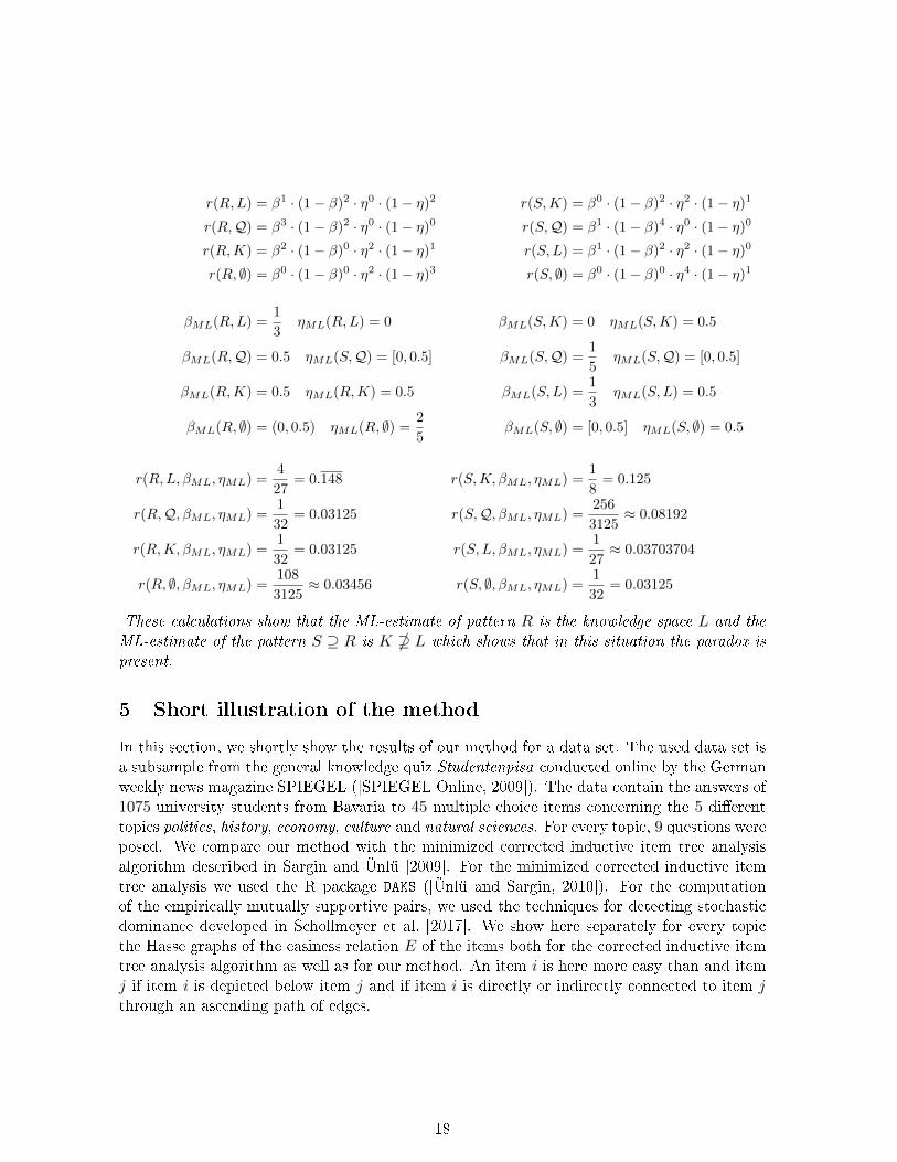
For the knowledge space (Q,K) with Q = q1, . . . , q5 and K = ∅,K := q3, q5, L :=q1, q2, q4,Q and the two response patterns R = q1, q4 and S = q1, q3, q4, q5 we cancompute the likelihood of observing such a response pattern (given a certain underlying trueknowledge space) under the most likely careless error and lucky guess probabilities from (4):

q1 q2 q3 q4 q5

Q x x x x xK x xL x x x∅R x xS x x x x

17

r(R,L) = β1 · (1− β)2 · η0 · (1− η)2 r(S,K) = β0 · (1− β)2 · η2 · (1− η)1

r(R,Q) = β3 · (1− β)2 · η0 · (1− η)0 r(S,Q) = β1 · (1− β)4 · η0 · (1− η)0

r(R,K) = β2 · (1− β)0 · η2 · (1− η)1 r(S,L) = β1 · (1− β)2 · η2 · (1− η)0

r(R, ∅) = β0 · (1− β)0 · η2 · (1− η)3 r(S, ∅) = β0 · (1− β)0 · η4 · (1− η)1

βML(R,L) =1

3ηML(R,L) = 0 βML(S,K) = 0 ηML(S,K) = 0.5

βML(R,Q) = 0.5 ηML(S,Q) = [0, 0.5] βML(S,Q) =1

5ηML(S,Q) = [0, 0.5]

βML(R,K) = 0.5 ηML(R,K) = 0.5 βML(S,L) =1

3ηML(S,L) = 0.5

βML(R, ∅) = (0, 0.5) ηML(R, ∅) =2

5βML(S, ∅) = [0, 0.5] ηML(S, ∅) = 0.5

r(R,L, βML, ηML) =4

27= 0.148 r(S,K, βML, ηML) =

1

8= 0.125

r(R,Q, βML, ηML) =1

32= 0.03125 r(S,Q, βML, ηML) =

256

3125≈ 0.08192

r(R,K, βML, ηML) =1

32= 0.03125 r(S,L, βML, ηML) =

1

27≈ 0.03703704

r(R, ∅, βML, ηML) =108

3125≈ 0.03456 r(S, ∅, βML, ηML) =

1

32= 0.03125

These calculations show that the ML-estimate of pattern R is the knowledge space L and theML-estimate of the pattern S ⊇ R is K + L which shows that in this situation the paradox ispresent.

5 Short illustration of the method

In this section, we shortly show the results of our method for a data set. The used data set isa subsample from the general knowledge quiz Studentenpisa conducted online by the Germanweekly news magazine SPIEGEL ([SPIEGEL Online, 2009]). The data contain the answers of1075 university students from Bavaria to 45 multiple choice items concerning the 5 dierenttopics politics, history, economy, culture and natural sciences. For every topic, 9 questions wereposed. We compare our method with the minimized corrected inductive item tree analysisalgorithm described in Sargin and Ünlü [2009]. For the minimized corrected inductive itemtree analysis we used the R package DAKS ([Ünlü and Sargin, 2010]). For the computationof the empirically mutually supportive pairs, we used the techniques for detecting stochasticdominance developed in Schollmeyer et al. [2017]. We show here separately for every topicthe Hasse graphs of the easiness relation E of the items both for the corrected inductive itemtree analysis algorithm as well as for our method. An item i is here more easy than and itemj if item i is depicted below item j and if item i is directly or indirectly connected to item jthrough an ascending path of edges.

18

topic: Politics

item analysis based on knowledge space theory (IITA algorithm of R package DAKS):

strongest empirically mutually supportive pair (item easiness relation E):

19

topic: History



20

topic: Economy



21

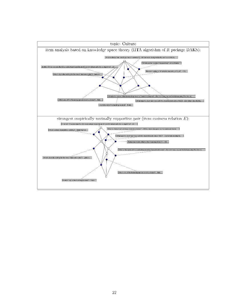
topic: Culture



22

topic: Natural sciences



23

For our concrete data example, the item easiness relation E of the strongest empiricallymutually supportive pair seems to be tendentially stronger than the relation obtained fromthe inductive item tree analysis. If this is only a coincidence or if this has some reason seemsto be not so clear. A further natural question one could ask is how our method statisticallybehaves under some presumed item response model. Also this question seems to be verydicult to answer in the general multidimensional situation. However, for the case thatone has a nite and xed number of items that are uniformly strictly totally ordered w.r.t.diculty (meaning that for two dierent items there is always one item which has smallersolving probabilities, no matter, which person tries to solve it) one can show that if wesample from a population and let the number of sampled persons tend to innity, then theprobability that the observed easiness relation diers from the true diculty relation goes tozero. The reason for this consistency property is the following:

For two items mi and mj where mi is easier than mj , the strongest empirically mutuallysupportive pair will declare mi as easier than mj if one can nd an appropriate matching ofpersons. To see that if only n is large enough, with arbitrary high probability one will ndsuch a matching, divide the set of all observed response patterns in all dierent classes wherethe responses to all items except the responses to the item mi and mj are identical. If nis large enough, then with high probability, in every such class the ordinal relations amongthe observed frequencies of the dierent patterns are identical to the ordinal relations amongthe true probabilities. This means in particular, that with high probability, in every classone observes more persons that solved mi and not mj than persons, who solved mj but notmi. This means that we can nd a matching of persons who solved answers as following: Inevery class, match persons, who solved both items to itself and match persons, who solvedmj but not mi to persons who solved mi but not mj , which is possible, because there aremore persons, who solved mi but not mj than persons who solved mj but not mi. To see thatthis matching is showing that mi is easier than mj due to the strongest empirically mutuallysupportive pair, we have to make sure that we have matched persons only to persons who areless successful, but this is clear, because the matched persons did solve the same items up toitem mi and mj and item mi was easier than item mj due to the easiness relation given inthe rst step of the application of the operator L.

6 Conclusion

In this paper we have developed a purely descriptive and relational notion of item dicultyand person success. This notion avoids the paradox described in Hooker et al. [2009]. We alsoshortly indicated, how the descriptive method statistically behaves under certain univariatepresumed models of item response theory. For multidimensional models, the behavior ofthe method seems to be far from clear. Furthermore, also the behavior of the method incomparison to descriptive methods like item tree analysis has still to be further studied.

References

Bolt, D. (2007). The present and future of IRT-based cognitive diagnostic models (ICDMs)and related methods. Journal of Educational Measurement, 44(4):377383.

24

de la Torre, J. (2009). Dina model and parameter estimation: A didactic. Journal of Educa-tional and Behavioral Statistics, 34(1):115130.

De Schuymer, B., De Meyer, H., and De Baets, B. (2003a). A fuzzy approach to stochasticdominance of random variables. In Bilgiç, T., Baets, B. D., and Kaynak, O., editors, TenthInternational Fuzzy Systems Association World Congress, pages 253260. Springer.

De Schuymer, B., De Meyer, H., De Baets, B., and Jenei, S. (2003b). On the cycle-transitivityof the dice model. Theory and Decision, 54(3):261285.

DiBello, L. V. and Stout, W. (2007). Guest editors' introduction and overview: IRT-basedcognitive diagnostic models and related methods. Journal of Educational Measurement,44(4):285291.

Doignon, J. and Falmagne, J. (2012). Knowledge Spaces. Springer.

Doignon, J.-P. and Falmagne, J.-C. (1985). Spaces for the assessment of knowledge. Interna-tional Journal of Man-Machine Studies, 23(2):175 196.

Falmagne, J. and Doignon, J. (2010). Learning Spaces: Interdisciplinary Applied Mathematics.Springer.

Falmagne, J.-C., Koppen, M., Villano, M., and Doignon, J.-P. (1990). Introduction to know-ledge spaces: How to build, test, and search them. Psychological Review, 97(2):201224.

Finkelman, M. D., Hooker, G., and Wang, Z. (2010). Prevalence and magnitude of paradoxicalresults in multidimensional item response theory. Journal of Educational and BehavioralStatistics, 35(6):744761.

Heller, J., Stefanutti, L., Anselmi, P., and Robusto, E. (2015). On the link between cognitivediagnostic models and knowledge space theory. Psychometrika, 80(4):9951019.

Hooker, G., Finkelman, M., and Schwartzman, A. (2009). Paradoxical results in multidimen-sional item response theory. Psychometrika, 74(3):419442.

Humphry, S. M. (2013). A middle path between abandoning measurement and measurementtheory. Theory & Psychology, 23(6):770785.

Jordan, P. (2013). Paradoxien in quantitativen Modellen der Individualdiagnostik. PhD thesis,Universität Hamburg. URL http://ediss.sub.uni-hamburg.de/volltexte/2013/6198/.

Jordan, P. and Spiess, M. (2012). Generalizations of paradoxical results in multidimensionalitem response theory. Psychometrika, 77(1):127152.

Junker, B. W. and Sijtsma, K. (2001). Cognitive assessment models with few assumptions, andconnections with nonparametric item response theory. Applied Psychological Measurement,25(3):258272.

Kamae, T., Krengel, U., and O'Brien, G. L. (1977). Stochastic inequalities on partially orderedspaces. The Annals of Probability, 5(6):899912.

Lehmann, E. (1955). Ordered families of distributions. Ann Math Stat, 26:399419.

25

Levhari, D., Paroush, J., and Peleg, B. (1975). Eciency analysis for multivariate distributi-ons. The Review of Economic Studies, 42(1):8791.

Michell, J. (2008a). Conjoint measurement and the Rasch paradox. Theory & Psychology,18(1):119124.

Michell, J. (2008b). Is psychometrics pathological science? Measurement, 6(1-2):724.

Ünlü, A. and Sargin, A. (2010). Daks: An r package for data analysis methods in knowledgespace theory. Journal of Statistical Software, Articles, 37(2):131.

Popper, K. (2005). The Logic of Scientic Discovery. Taylor & Francis.

Rasch, G. (1977). On specic objectivity: An attempt of formalizing the generality andvalidity of scientic statements. Danish Yearbook of Philosophy, 14:5894.

Rusch, A. and Wille, R. (1996). Knowledge spaces and formal concept analysis. In Bock,H.-H. and Polasek, W., editors, Data Analysis and Information Systems: Statistical andConceptual Approaches Proceedings of the 19th Annual Conference of the Gesellschaft fürKlassikation e.V. University of Basel, pages 427436. Springer.

Sargin, A. and Ünlü, A. (2009). Inductive item tree analysis: Corrections, improvements, andcomparisons. Mathematical Social Sciences, 58(3):376 392.

Schollmeyer, G., Jansen, C., and Augustin, T. (2017). Detecting stochastic dominace forposet-valued random variables as an example of linear programming on closure systems.Technical Report 209, Department of Statistics, LMU Munich.

Schrepp, M. (1999). Extracting knowledge structures from observed data. British Journal ofMathematical and Statistical Psychology, 52(2):213224.

Schrepp, M. (2002). Explorative analysis of empirical data by boolean analysis of question-naires. Zeitschrift für Psychologie, 210(2):99109.

Sijtsma, K. (2012). Psychological measurement between physics and statistics. Theory &Psychology, 22(6):786809.

SPIEGEL Online (2009). Studentenpisa - Alle fragen, alle Antworten. In German. accessed18.08.2017.

Strassen, V. (1965). The existence of probability measures with given marginals. The Annalsof Mathematical Statistics, 36(2):423439.

Tatsuoka, C. (2002). Data analytic methods for latent partially ordered classication models.Journal of the Royal Statistical Society: Series C (Applied Statistics), 51(3):337350.

Tatsuoka, K. K. (1990). Toward an integration of item-response theory and cognitive errordiagnosis. In Frederiksen, N., Glaser, A., Lesgold, A., and Safto, M., editors, DiagnosticMonitoring of Skill and Knowledge Acquisition, pages 453488. Taylor & Francis.

Ünlü, A. and Sargin, A. (2010). DAKS: An R package for data analysis methods in knowledgespace theory. Journal of Statistical Software, 37(2):131.

26

Appendix

A Basics of formal concept analysis (FCA)

In formal concept analysis one has given a so-called formal context K = (G,M, I) where Gis a set of objects, M is a set of attributes and I ⊆ G ×M is a binary relation between theobjects and the attributes with the interpretation (g,m) ∈ I i object g has attribute m. If(g,m) ∈ I we also use inx notation and write gIm. A formal concept of the context K isa pair (A,B) of a set A ⊆ G of objects, called extent, and a set B ⊆M of attributes, calledintent, with the following properties:

1. Every object g ∈ A has every attribute m ∈ B (i.e.: ∀g ∈ A∀m ∈ B : gIm).

2. There is no further object g ∈ G\A that has also all attributes of B (i.e.: ∀g ∈ G :(∀m ∈ B : gIm) =⇒ g ∈ A).

3. There is no further attribute m ∈ M\A that is also shared by all objects g ∈ A (i.e.∀m ∈M : (∀g ∈ A : gIm) =⇒ m ∈ B).

Conceptually, the concept extent describes, which objects belong to the formal conceptand the intent describes, which attributes characterize the concept. The property of being aformal concept can be characterized with the following operators

Φ : 2M −→ 2G : B 7→ g ∈ G | ∀m ∈ B : gImΨ : 2G −→ 2M : A 7→ m ∈M | ∀g ∈ A : gIm

as(A,B) is a formal concept ⇐⇒ Ψ(A) = B & Φ(B) = A.

This can be verbalized as: The pair (A,B) is a formal concept i B is exactly the set ofall common attributes of the objects of A and A is exactly the set of all objects having allattributes of B.

On the set of all formal concepts one can dene a sub-concept relation as

(A,B) ≤ (C,D) ⇐⇒ A ⊆ C & B ⊇ D.

(Actually, for formal concepts the equivalence A ⊆ C ⇐⇒ B ⊇ D holds.) If the concept(A,B) is a sub-concept of (C,D) then it is a more specic concept containing less objectsthat have more attributes in common. The set of all formal concepts of a context K togetherwith the sub-concept relation is called the concept lattice. (The concept lattice is in fact acomplete lattice.)

A formal (attribute) implication is a pair (Y, Z) of subsets of M , also denoted byY −→ Z. We say that an implication Y −→ Z is valid in a context K if every intent of Kthat contains all elements of Y also contains all elements of Z. In this case we also say thatthe context K respects the implication Y −→ Z. A formal implication Y −→ Zis calledsimple if Y is a singleton.

27

B Basics of knowledge space theory (KST)

A knowledge structure is a tuple (Q,K) where Q is a set of questions (items) and K is afamily of subsets of Q that includes the empty set and the set Q. A set S ∈ K is called aknowledge state and models the items a person is able to master. Since mastering an item imay imply mastering an item j, some sets T ⊆ Q cannot occur as a knowledge state. The setK models the set of all possible knowledge states, a person could be in. A knowledge structure(Q,K) where K is closed under arbitrary unions is called a knowledge space. A knowledgespace where K is furthermore closed under arbitrary intersections is called a quasi ordinalknowledge space.

C Connections between FCA and KST

The connections between formal concept analysis and knowledge space theory are describedin Rusch and Wille [1996]. For a given knowledge space (Q,K) one can associate the formalcontext K := (G,Q, I), where G is a set of persons that answered the set Q of questionsand gIq means that person g did not solve question q. With this association of a formalcontext to a knowledge space we have a one to one correspondence between formal contextsand knowledge spaces. While knowledge spaces are closed under unions, the concept intentsof the associated formal contexts are the complements of the knowledge states and are closedunder intersection. A formal implication q −→ r could be interpreted as every person thatdid not solve item q also did not solve item r, which could also be stated as mastering item rimplies mastering item q.

D Basics of stochastic dominance

For two random variables X,Y on the same probability space (Ω,F , P ) and with values in apartially ordered set (V,≤) one says that X is weakly stochastically dominated by Y (w.r.t.rst order stochastic dominance) if there exist two copies X ′ and Y ′ on another probability

space (Ω′,F ′, P ′) with Xd= X ′, Y

d= Y ′ and P ′(X ′ ≤ Y ′) = 1. Stochastic dominance can

be characterized by the following, essentially equivalent conditions: The random variable Xis (weakly) stochastically smaller than the random variables Y if one of the three followingconditions is satised6:

i) P (X ∈ A) ≤ P (Y ∈ A) for every (measurable) upset A ⊆ V

ii) E(u X) ≤ E(u Y ) for every bounded non-decreasing borel-measurable7 function u :V −→ R

iii) It is possible to obtain the density8 fY from the density fX by transporting probabilitymass from values v to greater or equal values v′ ≥ v .

6The equivalence between (ii) and (i) was shown by Lehmann [1955] and independently proved by Levhariet al. [1975]. The equivalence between (iii) and (i) is a consequence of Strassen's Theorem ([Strassen, 1965]),see Kamae et al. [1977].

7Here, we have to assume that (V,≤) can be equipped with an appropriate topology that makes it a partiallyordered polish space.

8This statement is of course only equivalent if the densities fX and fY actually exist.

28

Characterization i) is more or less used in denition 1 of this paper, with the dierence thatone does not have a normalized probability measure P , but instead, a counting measure isunderlying. Characterization iii) is very close to the idea of dening a person X as lesssuccessful than person Y if one can match every item solved by person X to an item solvedby person Y that is at least as dicult.

29

Documents

A simple descriptive method for multidimensional item