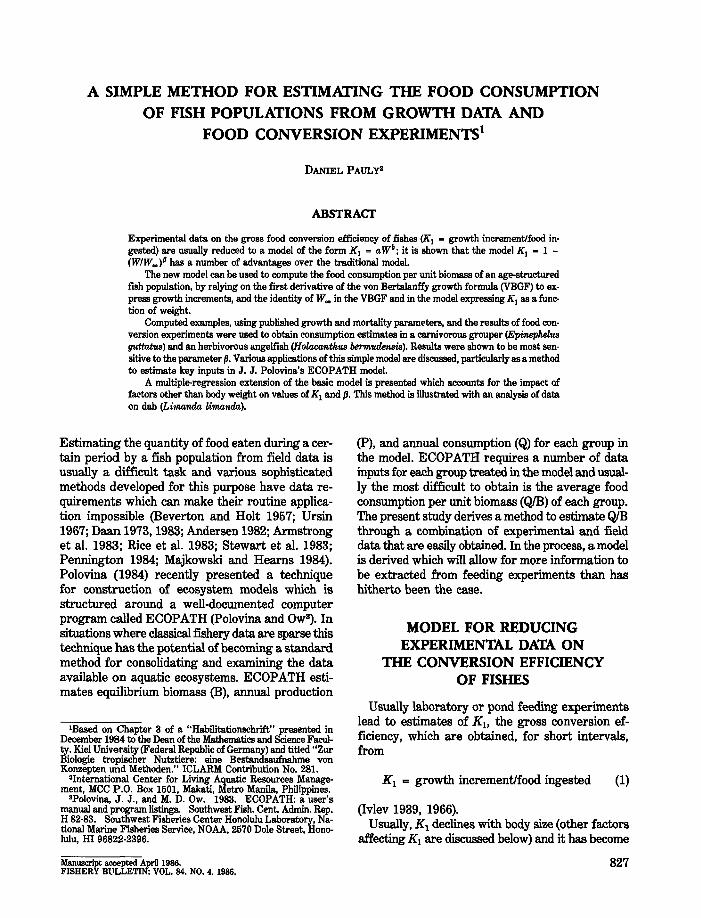
A SIMPLE METHOD FOR ESTIMATING THE FOOD CONSUMPTIONOF FISH POPULATIONS FROM GROWTH DATA AND

FOOD CONVERSION EXPERIMENTS}

DANIEL PAULy2

ABSTRACf

Experimental data on the gross food conversion efficiency of fishes (KI - growth increment/food in­gested) are usually reduced to a model of the form K I = aWb ; it is shown that the model K I = 1 ­(WIW_)~ has a number of advantages over the traditional model.

The new model can be used to compute the food consumption per unit biomass of an age-structuredfish population, by relying on the first derivative of the von Bertalanffy growth formula (VBGF) to ex­press growth increments, and the identity of W~ in the VBGF and in the model expressing KI as a func­tion of weight.

Computed examples, using published growth and mortality parameters, and the results of food con­version experiments were used to obtain consumption estimates in a carnivorous grouper (Epi'MPMI1Ul!J'I'ttatus) and an herbivorous angelfish (HolacantkU8 berm:uMlI8is). Results were shown to be most sen­sitive to the parameter (I. Various applications of this simple model are discussed, particularly as a methodto estimate key inputs in J. J. Polovina's ECOPATH model.

A multiple-regression extension of the basic model is presented which accounts for the impact offactors other than body weight on values of K I and (I. This method is illustrated with an analysis of dataon dab (Lil/la7lda limanda).

Estimating the quantity of food eaten during a cer­tain period by a fish population from field data isusually a difficult task and various sophisticatedmethods developed for this purpose have data re­quirements which can make their routine applica­tion impossible (Beverton and Holt 1957; Ursin1967; Daan 1973,1983; Andersen 1982; Armstronget al. 1983; Rice et al. 1983; Stewart et al. 1983;Pennington 1984; Majkowski and Hearns 1984).Polovina (1984) recently presented a techniquefor construction of ecosystem models which isstructured around a well-documented computerprogram called ECOPATH (Polovina and Ow8). Insituations where classical fishery data are sparse thistechnique has the potential of becoming a standardmethod for consolidating and examining the dataavailable on aquatic ecosystems. ECOPATH esti­mates equilibriwn biomass (B), annual production

I Based on Chapter 3 of a "Habilitationschrift" presented inDecember 1984 to the Dean of the Mathematics and Science Facul­ty, Kiel University (Federal Republic of Germany) and titled "ZurBiologie tropischer Nutztiere: eine Bestandsaufnabme vonKonzepten und Methoden." ICLARM Contribution No. 281.

"International Center for Living Aquatic Resources Manage­ment, MCC P.O. Box 1501, Makati, Metro Manila, Philippines.

'Polovina, J. J., and M. D.Ow. 1983. ECOPATH: a user'smanual and program listings. Southwest Fish. Cent. Admin. Rep.H 82-83. Southwest Fisheries Center Honolulu Laboratory, Na­tional Marine Fisheries Service, NOAA, 2570 Dole Street, Hono­lulu, HI 96822-2396.

Manuscript accepted April 1986.FISHERY BULLETIN: VOL. 84. NO.4. 1986.

(P), and annual consumption (Q) for each group inthe model. ECOPATH requires a nwnber of datainputs for each group treated in the model and usual­ly the most difficult to obtain is the average foodconswnption per unit biomass (Q1B) of each group.The present study derives a method to estimate Q1Bthrough a combination of experimental and fielddata that are easily obtained. In the process, a modelis derived which will allow for more information tobe extracted from feeding experiments than hashitherto been the case.

MODEL FOR REDUCINGEXPERIMENTAL DATA ON

THE CONVERSION EFFICIENCYOF FISHES

Usually laboratory or pond feeding experimentslead to estimates of K 1, the gross conversion ef­ficiency, which are obtained, for short intervals,from

K 1 = growth increment/food ingested (1)

(Ivlev 1939, 1966).Usually, K1 declines with body size (other factors

affecting K1 are discussed below) and it has become

827

FISHERY BULLETIN: VOL. 84, NO.4

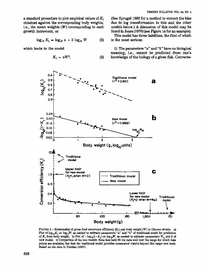
a standard procedure to plot empirical values of K1obtained against the corresponding body weights,Le., the mean weights (W) corresponding to eachgrowth increment, or

IOg10 K 1 = IOg10 a + b IOg10 W (2)

(See Sprugel1983 for a method to correct the biasdue to log transformation in this and the othermodels below.) A discussion of this model may befound in Jones (1976) (see Figure 1a for an example).

This model has three liabilities, the first of whichis the most serious:

which leads to the model

(3)

1) The parameters "a" and "b" have no biologicalmeaning, Le., cannot be predicted from one'sknowledge of the biology of a given fish. Converse-

Traditional model(r2 =0.821)

0.4

0.5

0.6

0.7

0.8

0.9

..... ..... .~ ............. -\.-.. ..... .....- ...............

......................

a

bNew model(r2 =0.888)

0.25

0.20

~ 0.15I-= 0.10 I Wo oQIO CD

6~ I.2 0.00 L- ..l..- ...L- ---:I::::...~ _

I 0 2 3

Body weight (g t loglounits)

Traditional

\el

----.ex>

c

•1,500

---- Traditional model

-- New model

100 150

Body weight(g)50

Lower limitfor new model

.....-O:.r''''r--jj.;-~.~_=.- .................=~[","0 ....Wjw",l

'" Traditional/ model

IIIIII Upper limitI for new model

1.0 - (KI=I,when W=O)

0.4

0.2

0.6

>­ucCD

"(3~­CDCo

"ijj...~co

CJ

FIGURE l.-Relationship of gross food conversion efficiency (Kl) and body weight (W) in Channa. striata. a)Plot of 10glOKl on 10glOW, as needed to estimate parameters "a" and "b" of traditional model for predictionof K l from body weight. b) Plot of -loglO(l-Kl) on 10glOW, as needed to estimate parameters W~ and p ofnew model. c) Comparison of the two models. Note that both fit the data well over the range for which datapoints are available, but that the traditional model provides nonsensical results beyond this range (see text).Based on the data in Pandian (1967).

828

PAULY: ESTIMATING FOOD CONSUMPTION OF FISH POPULATIONS

C = (J IOglO ~ - (J IOglO W (5)

with (J as a constant and ~ as the weight at whichK I = 0. The model implies that K I = 1 when W =0, whatever the values of (J and ~ (see Discussionfor comments on using values other than 1 as up­per bound for K I in Equation (4». The new modelcan, as the traditional model, be fitted by means ofa double logarithmic plot:

ly, these parameters do not provide informationwhich can be interpreted via another model.

2) The model implies values of K I > 1 when a-lib

>W > 0, which is nonsensical.3) The model implies that, except when W = 0,

K I is always> 0, even in very large fish, althoughit is known that fish cannot grow beyond certainspecies-specific and environment-specific sizes,whatever their food intake.

The new model proposed here has the form

K I = 1 - (W/~)/l (4)

where C = -IOglO (1 - K I ), the sign being changedhere to allow the values of C to have the same posi­tive sign as the original values of K I • Interesting­ly, it also appears that negative values ofK I (basedon fish which lost weight), which must be ignoredin the traditional model, can also be used in thismodel (as long as they do not drag the mean of allavailable K I values below zero, see Table 1),although their interpretation seems difficult.

The new model requires no more data, normarkedly more computations than the old one. Itproduces "possible" values of KI over the wholerange of weights which a given fish can take. Thevalues of ~, which represent the upper bound ofthis range can be estimated from

~ = antiloglo (C interceptI IslopeI). (6)

Thus, while (J has no obvious biological meaning,the values of~ obtained by this model do have abiological interpretation, which is, moreover, anal­ogous to the definition of~ in the von Bertalanffygrowth function (VBGF) of the form

TABLE 1.-0ata on the food conversion efficiency of Channa slriata (= Ophiocepha/usstriatus) (after Pandian 1967). Epinephelus strlatus (after Menzel 1960), and HoIa-canthus bermudansis (after Menzel 1958).

Body Food Transformed data Speciesweight conv. C = and

(g)1 (K,P log,o W log,oK, -log,o(l - K,) remarks

1.86 0.391 0.270 -0.408 0.2159.92 0.274 0.998 -0.562 0.139

13.09 0.320 1.117 -0.495 0.16719.65 0.284 1.293 -0.547 0.14724.63 0.278 1.391 -0.556 0.14135.09 0.234 1.545 -0.631 0.11645.15 0.199 1.655 -0.701 0.096 Channa striata50.70 0.227 1.705 -0.644 0.112 (see Figure 1)51.30 0.235 1.710 -0.629 0.11657.00 0.208 1.756 -0.682 0.10179.80 O.ln 1.897 -0.752 0.08593.80 0.232 1.972 -0.635 0.115

107.50 0.157 2.031 -0.804 0.074123.60 0.166 2.093 -0.780 0.079

216 0.247 2.334 -0.607 0.123

I285 0.219 2.455 -0.600 0.107 Epinephelus319 0.160 2.504 -0.796 0.076 guttatus;392 0.153 2.593 -0.815 0.072 ~,o W = 2.617;424 0.179 2.627 -0.747 0.086 C = 0.0894628 0.161 2.798 -0.793 0.076 (see Figure 2)647 O.ln 2.811 -0.752 0.065649 0.187 2.812 -0.728 0.090

68 0.222 1.820 -0.654 0.109 } Ho/acanthus139 0.178 2.143 -0.750 0.085 bermudansis256 -0.258 2.408 not de- -0.100 (280C only)3

fined I!?g,o W = 2.124C = 0.031

1Mean of starting and end weights.'Growth Incrementlfood intake.3Nots that the experiment considered here was conducted with a food which led to depoa~ion

of lat. but not of protein (see also Table 2), a consideratlon that Is ignored lor the sake of this example.

829

FISHERY BULLETIN: VOL. 84, NO.4

(7) of the example here, one obtains with r = 0.942 anew model:

(von Bertalanffy 1938; Beverton and Holt 1957), andwhere WI> the weight at time t, is predicted via theconstants K, to, and l¥.." all three of which areusually estimated from size-at-age data obtained inthe field (see Gulland 1983 or Pauly 1984a).

That 1¥.. values obtained via Equations (2) and (6)are realistic can be illustrated by means of that partof the data in Table 1 pertaining to Channa striata(= Ophiocephalus striatus), the "snakehead" or"mudfish" of south and southeast Asia. These datagive, when fitted to the traditional model

K I = O.482W-O.205. (8)

K 1 = 1 - (WIl,290)o.o77 (12)

close to that obtained using a Type I regression, dueto the high value of r of this example. However, incases where the fit to the model is poor, the use ofa Type II regression can make all the differencebetween realistic and improbable values of l¥..,.

Another approach toward optimal utilization ofthe properties of the new model (4) is the use of "ex­ternal" values of asymptotic weight, which will herebe coded "Wc'",) to differentiate them from values ofl¥.., estimated through the model. In such case, {Jcan be estimated from

The same data, when fitted to the new model give

1) the 10glO W values are not controlled by theexperimentator and

2) regression parameters are required, ratherthan prediction of C values (see Ricker 1973).

(See Figure 1 for both models.) The value of l¥.., =1,580 g is low for a fish which can reach up to 90em in the field (Bardach et al. 1972). However, itsgrowth may have been reduced in laboratory growthexperiments conducted by Pandian (1967).

Equation (6) used here to predict l¥.., is extreme­ly sensitive to variability in the data set investigated,and two approaches are discussed to deal with thisproblem.

The first approach is the appropriate choice of theregression model used. In the example above (Equa­tion (9», the model used was a Type I (predictive)regression, which is actually inappropriate, giventhat

K 1 = 1 - (WIl,880)o.136 (14)

(13)(J = CIQOglO '"I",) - 10glO W)

in which "f",j is an asymptotic size estimated fromother than food conversion and weight data, e.g.,from growth data or via the often observed close­ness between estimates of asymptotic size and themaximum sizes observed in a given stock (see Pauly1984a, chapter 4).

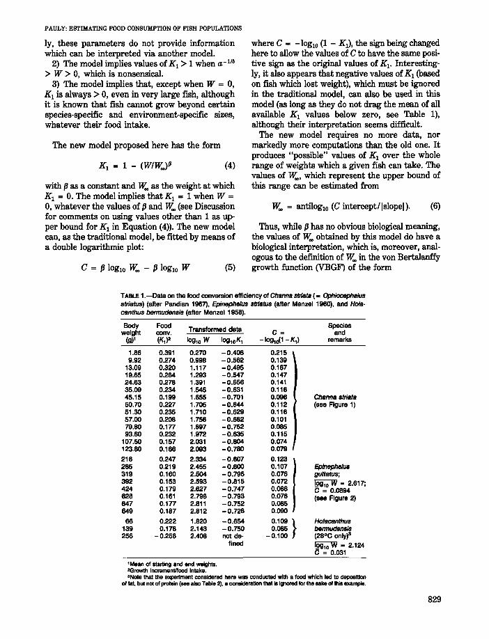
These two approaches are illustrated in the exam­ple below, which is based on the data in Table 1 per­taining to the grouper Epinephelus guttatus. WhenEquation (6) is interpreted as a Type I regression,these data yield a value of 1¥.. >12 kg, which is fartoo high for a fish known to reach 55 cm at most(Randall 1968). Interpreting Equation (5) as a TypeII regression leads to a value of l¥.., = 3.5 kg whichis realistic, although still not close to the asymptoticweight of 1,880 g estimated by Thompson andMunro (1977). Finally, using the latter figure as anestimate of "foo) yields the model

(9)K I = 1 - (WIl,580)0.D73.

The use of a Type II ("functional", or "GeometricMean") regression appears more appropriate; con­version of a Type I to Type II regression (withparameters a', b') can be performed straight­forwardly through

as a description of the relationship between K 1 andweight in Epinephelus guttatus (Fig. 2). The valueof {J in Equation (14) lies within the 95% confidenceinterval of the value of {J = 0.060 which generatedthe first unrealistically high estimate of l¥..,.

where r is the correlation coefficient between theC and the IOglO Wvalues (Ricker 1973). In the case

830

and

b' = bllrl

a' = C - b' 10glO W

(10)

(11)

MODEL FOR ESTIMATINGTHE FOOD CONSUMPTION

OF FISH POPULATIONS

When feeding experiments have been or can beconducted under conditions similar to those prevail­ing in the sea (food type, temperature, etc.), the

PAULY: ESTiMATING FOOD CONSUMPTION OF FiSH POPULATIONS

3.5 4D

_._._ w.. estimated throughType I regression

W", estimated through-- Type II regression

.. Mean of y, x values

____ WI"" inputfrom outside

3.0

•~ .,\~., .........

\ ........., '-.\ ........., ........, ........" ........., '-.

\ 1DQIO'\,ITVpeKI......... I~TVP'II\ /' '-. 7

• •

2.5

o.oe~-

I

~ Q06

0"j

Q04

0.02

aoo20

Body weight (g ,log1ounits)

FIGURE 2.-Relationship between gross food conversion efficiency (K1I and body weight inEpineph.eltls guttahUl. Note that a Type I "predictive" regression leads to an overestimationof W~ while a Type II "functional" regression leads to a value of W~ close to an estimateof W~ based on growth data (see text). Based on data in Menzel (1960).

Kl(O = 1 - (1 - e-K (t- 1ol)8/l (15)

where Kl(t) is the food conversion efficiency of theinvestigated fish as a function of their age t, andK, to, and (J are as defined above.

Equation (1) is then rewritten as

where the "growth increment" is replaced. by agrowth rate (dw/dt) and the "food ingested" is alsoexpressed as a rate (dq/dt). The growth rate of thefish is then expressd by the first derivative of theVBGF (Equation (7» or

dw/dt = ~ 3K (1 - exp( -Kri»2 . exp( -Kr1) (17)

(19)

where tr is the age at recruitment (i.e., the startingage at which Z applies, assuming, if there is anyfishery, that tr = tc' the mean age at first capture),R the number of recruits, and Nt is the number offish in the population. As the model below assumesa stationary population, the food consumption of thepopulation per unit time can be expressed on a per­recruit basis or

Q- = W 3KR '"

The food consumption of a population should de­pend, on the other hand, on the age structure of thatpopulation. The simplest way to impose an age struc­ture on a population is to assume exponential decaywith instantaneous mortality Z, or

tmax

Q = w: 3Kf(1 - exp(-Kr1»2. exp(-Kr1) dt.c '" 1 - (1 - exp( -K?'l» 8/1

Ir (18)

(16)dq/dt = (dw/dt)/K1(t)

model presented above can be made a part of amodel for estimation of food consumption per unitbiomass (Q/B), provided a set of growth parametersis also used in which the value of~ or U("'I is iden­tical to that estimated from or used to interpret thefeeding experiments.

In this case, inserting Equation (8) into Equation(5) leads to

where rl = t - to' Equations (17) and (15) may besubstituted into Equation (16), which is a separabledifferential equation and may be solved by direct in­tegration. The cumulative food consumption of anindividual fish between the age at recruitment (tr )

and the age at which it dies (tmax) is thus

- exp( -Krl»2 . exp( -(Krl + Zr2» dt1 - (1 - exp( -Krl»8/l

(20)

831

where r2 = t - tr •

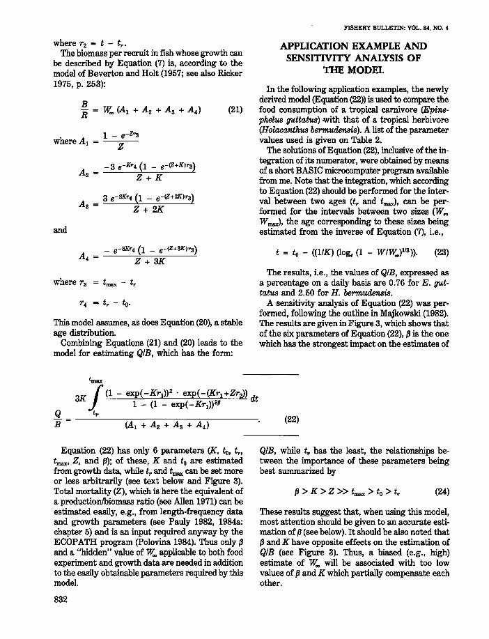
The biomass per recruit in fish whose growth canbe described by Equation (7) is, according to themodel of Beverton and Holt (1957; see also Ricker1975, p. 253):

BR = lv.., (AI + A 2 + As + A 4 ) (21)

1 - e-Zrswhere Al = Z

and

FISHERY BULLETIN: VOL. 84. NO.4

APPLICATION EXAMPLE ANDSENSITIVITY ANALYSIS OF

THE MODEL

In the following application examples, the newlyderived model (Equation (22» is used to compare thefood consumption of a tropical carnivore (Epine­phelus guttatus) -with that of a tropical herbivore(Holacanthus bermudensis). A list of the parametervalues used is given on Table 2.

The solutions of Equation (22), inclusive of the in­tegration of its numerator, were obtained by meansof a short BASIC microcomputer program availablefrom me. Note that the integration, which accordingto Equation (22) should be performed for the inter­val between two ages (tr and tmax), can be per­formed for the intervals between two sizes (Wr ,

Wmax), the age corresponding to these sizes beingestimated from the inverse of Equation (7), i.e.,

- e-SKr4 (1 _ e-IZ+3Klrs)

A 4 = Z + 3Kt = to - «11K) (log, (1 - WIlv..,)I/S». (23)

where r 3 = tmax - tr

This model assumes, as does Equation (20), a stableage distribution.

Combining Equations (21) and (20) leads to themodel for estimating QIB, which has the form:

Equation (22) has only 6 parameters (K, to, tr ,

tmax, Z, and (j); of these, K and to are estimatedfrom growth data, while tr and tmax can be set moreor less arbitrarily (see text below and Figure 3).Total mortality (Z), which is here the equivalent ofa productionlbiomass ratio (see Allen 1971) can beestimated easily, e.g., from length-frequency dataand growth parameters (see Pauly 1982, 1984a:chapter 5) and is an input required anyway by theECOPATH program (Polovina 1984). Thus only {jand a "hidden" value of lv.., applicable to both foodexperiment and growth data are needed in additionto the easily obtainable parameters required by thismodel.

832

The results, i.e., the values of QIB, expressed asa percentage on a daily basis are 0.76 for E. gut­tatus and 2.50 for H. bermudensis.

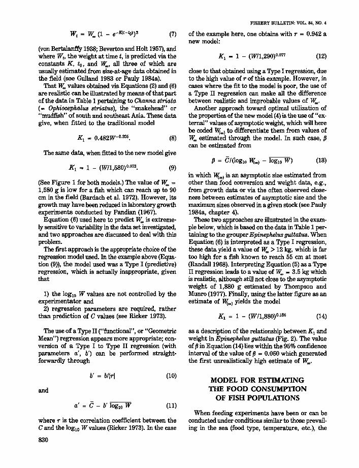
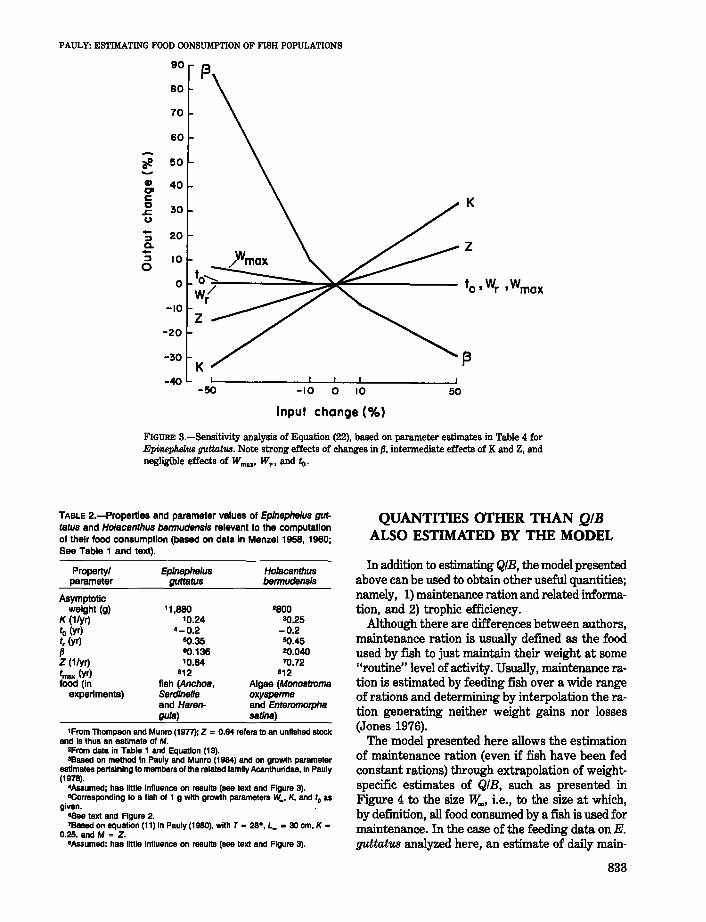
A sensitivity analysis of Equation (22) was per­formed, following the outline in Majkowski (1982).The results are given in Figure 3, which shows thatof the six parameters of Equation (22), {j is the onewhich has the strongest impact on the estimates of

(22)

QIB, while tr has the least, the relationships be­tween the importance of these parameters beingbest summarized by

{j > K >Z » tmax > to > tr (24)

These results suggest that, when using this model,most attention should be given to an accurate esti­mation of {j (see below). It should be also noted that{j and K have opposite effects on the estimation ofQIB (see Figure 3). Thus, a biased (e.g., high)estimate of lv.., will be associated with too lowvalues of {j and K which partially compensate eachother.

PAULY: ESTIMATING FOOD CONSUMPTION OF FISH POPULATIONS

80

70

60

*" 50

CD 40C'cc 30.s::.u- 20:JQ.-:J 100

0

-10

-20

-30K

-40-50 -10 0 10

Input change (%)

50

FIGURE S.-Sensitivity analysis of Equation (22), based on parameter estimates in Table 4 forEpinephelus guttatus. Note strong effects of changes in fJ, intermediate effects of K and Z, andnegligible effects of Wmax' WT , and to.

TABLE 2.-Properties and parameter values of Epinephelus gut­tatus and Holacanthus bermudensis relevant to the computationof their food consumption (based on data in Menzel 1958, 1960;See Table 1 and text).

'From Thompson and Munro (1977); Z = 0.64 refers to an unfished atockand Is thus an estimate 01 M.

"From data in Table 1 and Equation (13)."Basad on method in Pauly and Munro (1984) and on growth parameter

estimates pertaining to members of the related family Acanthuridae, In Pauly(1976).

"Assumed; has little influence on results (see teX1 and Figure 3)."Corresponding to a fish of 1 g with growth parameters W., K, and f. as

given.°Sse text and Figure 2.7Based on equation (11) in Pauly (1980), with T • 26°, L. = 30 em, K •

0.25. and M = Z.oAssumed: has little Influence on results (sse teX1 and Figure 3).

Propertylparameter

Asymptoticweight (g)

K (l/yr)to (yr)t, (yr)fJZ (l/yr)tmax (yr)food (in

experiments)

Epinephelusguttatus

11,88010.24

4-0.250.3580.13610.64

812fish (Anchoa,Sardlne//aand Haren­gula)

Ho/acanthusbermudensis

28003Q.25

-0.250.4520.04070.72

812Algae (Monostromaoxyspermaand Enteromorphasatina)

QUANTITIES OTHER THAN QIBALSO ESTIMATED BY THE MODEL

In addition to estimating QIB, the model presentedabove can be used to obtain other useful quantities;namely, 1) maintenance ration and related informa­tion, and 2) trophic efficiency.

Although there are differ~ncesbetween authors,maintenance ration is usually defined as the foodused by fish to just maintain their weight at some"routine" level of activity. Usually, maintenance ra­tion is estimated by feeding fish over a wide rangeof rations and determining by interpolation the ra­tion generating neither weight gains nor losses(Jones 1976).

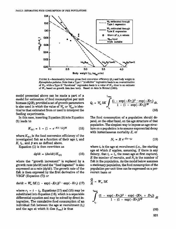
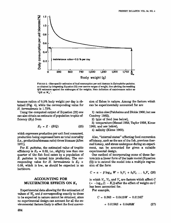
The model presented here allows the estimationof maintenance ration (even if fish have been fedconstant rations) through extrapolation of weight­specific estimates of QIB, such as presented inFigure 4 to the size lY.." Le., to the size at which,by definition, all food consumed by a fish is used formaintenance. In the case of the feeding data on E.guttatus analyzed here, an estimate of daily main-

833

FISHERY BULLETIN: VOL. 84. NO.4

0.4

0.6

0.2

w..1,7501,5001,2501,000750500250

maintenance ration =0.5 % per day

o

ii 1.2-gjoS 1.0

:ii§ Q8

~Q)a.5aE::Jenc:ou~"0c

Body weight (g)

FIGURE 4.-Size-specific estimates of food consumption per unit biomass in Epinephel!1S g",ttatw,as obtained by integrating Equation (22) over narrow ranges of weight, then plotting the resultingQlB estimates against the midranges of the weights. Note definition of maintenance ration as"QlB at W~".

tenance ration of 0.5% body weight per day is ob­tained (Fig. 4), while the corresponding value forH. bermudensis is 1.73%.

Using the computed output of Equation (22) onecan also obtain an estimate of population trophic ef­ficiency (ET) from

which expresses production per unit food consumed,production being expressed here as total mortality(Le., productionlbiomass ratio) times biomass (Allen1971).

For E. flI.'ttatus, the estimated value of trophicefficiency is ET = 0.23, i.e., slightly less than onequarter of the fish food eaten by a population ofE. guttatus is turned into production. The cor­responding value for H. bermudensis is ET =0.08, which is low, as should be expected in anherbivore.

ET = Z . (BIQ) (25)

sion of fishes in nature. Among the factors whichcan be experimentally accounted for are

1) ration size (Paloheimo and Dickie 1966; but seeCondrey 1982),

2) type of food (see below),3) temperature (Menzel 1958, Taylor 1958, Kinne

1960, and see below),4) salinity (Kinne 1960).

Also, "internal states" affecting food conversionefficiency, such as the sex of the fish, previous ther­mal history, and stress undergone during an experi­ment, can be accounted for given a suitableexperimental design.

One method of incorporating some of these fac­tors into a linear form of the basic model (Equation(5» is to extend the model into a multiple regres­sion of the form

in which VI' V2, and V" are factors which affect C{= -IOgIO (I - K 1»after the effect of weight on Chas been accounted for.

For example,

ACCOUNTING FORMULTIFACfOR EFFECtS ON K J

Experimental data allowing for the estimation ofvalues of Jv... and (J corresponding exactly to thoseto be expected in nature cannot be obtained, sinceno experimental design can account for all the en­vironmental factors likely to affect the food conver-

C = 0.363 - 0.0419W - 0.01l6T

+ 0.01568 + 0.0488M (27)

834

PAULY: ESTIMATING FOOD CONSUMPTION OF FISH POPULATIONS

(28)

4) Compute the intercept of the new Type II

1) Compute the parameters ofn + 1 Type I multi­ple regressions, where each regression (j) hasanother variable as dependent variable (i.e., Y, thenYI , Y2, ••• to Y,,; see j = 1 to 5 in Table 4).

2) Solve each of the j equations for the "real"dependent variable (Y = C, seej = 6 to 10 in Table4).

3) Compute the geometric mean of each partialregression coefficient from

(29)

This equation implies that there is, for every com­bination of VI' V2, ••• V" values, a correspondingvalue of lY... This is reasonable, as it confirms thatlY.. is environmentally controlled (Taylor 1958;Pauly 1981, 1984b). lY..-values obtained throughEquation (31) will generally be reliable-as was thecase with the one-factor model (4)-only when a widerange of weights are included, variability is low, andthe correct statistical model is used.

As a first approach toward an improved statisticalmodel, one could conceive of a geometric meanmultiple regression which, in analogy to a simplegeometric mean regression, would be derived fromthe geometric mean of the parameters of a seriesof multiple regressions. This approach would in­volve, in the case of n + 1 variables (= Y, Yh Y2,

. .. Y,,) in the following steps:Source of Degrees Sum of Meanvariation of freedom squares squares

Regression 4 0.0813 0.0203Residual 57 0.0516 0.0009

Total 61 0.1329

F(4.57) 22.465 P < 0.001

multiple correlation = 0.7822R 2 .. 0.6119Corrected R 2 = 0.5846Standard error = 0.0301

Variable Coefficient SE P

Weight -0.041669 -3.926 0.0107 <0.001Temp -0.011584 -7.362 0.0016 <0.001Sex 0.015635 1.982 0.0079 0.049Meat 0.048840 5.301 0.0092 <0.001Constant 0.363416

TABLE 3.-Details of a Type I multiple regression to quan·tify the effects of some factors on the food conversionefficiency of dab (UmandB Iimsnds) (see text footnote 3).

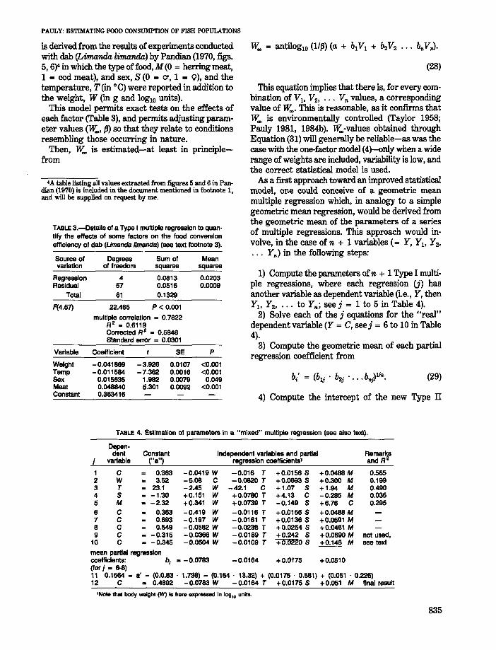
is derived from the results of experiments conducted.with dab (Limarula limarula) by Pandian (1970, figs.5, 6)4 in which the type of food, M (0 = herring meat,1 = cod meat), and sex, S (0 = cr, 1 = 9), and thetemperature, T (in 0c) were reported in addition tothe weight, W (in g and lOglO units).

This model permits exact tests on the effects ofeach factor (Table 3), and permits adjusting param­eter values (lY.., (3) so that they relate to conditionsresembling those occurring in nature.

Then, lY.. is estimated-at least in principle­from

'A table listing all values extracted from figures 5 and 6 in Pan­dian (1970) is included in the document mentioned in footnote 1,and will be supplied on request by me.

TABLE 4. Estimation of parameters in a "mixed" multiple regression (see also text).

Depen-dent Constant Independent variables and partial Remarks

j variable ("a") regression coefficients' and R 2

1 C 0.363 -0.0419 W -0.016 T +0.0156 S +0.0488 M 0.5652 W 3.52 -5.06 C -0.0620 T +0.0693 S +0.300 M 0.1993 T 23.1 -2.45 W -42.1 C +1.07 S +1.94 M 0.4904 S -1.30 +0.151 W +0.0780 T +4.13 C -0.285 M 0.0355 M .. -2.32 +0.341 W +0.0739 T -0.149 S +6.76 C 0.2956 C 0.363 -0.419 W -0.0116 T +0.0156 S +0.0488 M7 C 0.693 -0.197 W -0.0161 T +0.0136 S +0.0591 M8 C 0.549 -0.0582 W -0.0238 T +0.0254 S +0.0461 M9 C -0.315 -0.0366 W -0.0189 T +0.242 S +0.0890 M not used.

10 C .. -0.345 -0.0504 W -0.0109 T +0.0220 S +0.148 M see text

mean partial regressioncoefficients: b; ... -0.0783 -0.0164 +0.0175 +0.0510(for j .. 6-8)"11 0.1564 = a' - (0.0.83 . 1.738) - (0.164 . 13.32) + (0.0175 . 0.581) + (0.051 . 0.226)12 C ... 0.4892 -0.0783 W -0.0164 T +0.0175 S +0.051 M final result

'Note that body _ight (W);s here expl'88S8d in log,. units.

835

FISHERY BULLETIN: VOL. 84. NO.4

with both values of (J within the 95% confidenceinterval of the first estimate of (J (in Equation (27),see Table 3).

In the present case, this leads to (J values of 0.073and 0.089 for females and male dab, respectively.The "average" relationship (if such exists) betweenfood conversion efficiency and body weight in femaledab fed herring meat is thus

(35)

(36)

K 1 = 1 - (WI756)o.073

K 1 = 1 - (WI149)o.o89

while for males it is

500 g for the females and 298 g for the males, com­pared with the values of 756 and 149 g obtained byLee (1972) on the basis of growth studies.

Estimating values of (J that are wholly compatiblewith the latter estimates of w:. is straightforward,however, since it consists of solving Equation (31)for T = 18°C, M = 0, and the appropriate value of8, based on the equation

multiple regression from

where the Yi are the means of the Yi-values andbi the geometric mean partial regression coeffi­cients.

This method cannot be used here without modi­fication because in most cases the multiple regres­sion is "mixed" (Raasch 1983), consisting of vari­ables which can be expected to generate normallydistributed residuals when used as dependent vari­ables (here: C, W, T) as well as "dummy" or binaryvariables (8, M) which cannot generate normallydistributed residuals when they are used as depen­dent variables.

As might be seen in Table 4, the use of dummyvariables as "dependent" variables generates un­stable interrelationships between the remainingvariables, making the computation of meaningfulmean partial regression coefficients impossible.

The best solution here seems to omit for the com­putation of the mean regression coefficient thosemultiple regressions which have binary variables as"dependent" variables; Table 4 illustrates thisapproach.

The mixed model so obtained is

C = 0.489 - 0.0738W - 0.0164T + 0.01758DISCUSSION

C' = 0.62W' - 0.90T + 0.198' + 0.46M (32)

in which the original variables C, W, T,8, and Mare expressed in standard deviation units and inwhich the slopes (= path coefficients, see Li 1975)allow for comparing the effects of W, T, 8, and Mon C. These variables suggest that with regards totheir impact on C,

See Li (1975) for further inferences based on pathcoefficients.

In the southern North Sea in late summer-earlyautumn, Limanda limanda experiences tempera­tures usually ranging between 10° and 20°C (Lee1972). Solving Equation (31) for T = 18°C, thehighest temperature in Pandian's experiments (Le.,assuming the higher late summer-early autumntemperatures limit w:.) leads to estimates of w:. =

836

+ 0.0151M

which corresponds to the standard model

T> W>M»8.

(31)

(33)

The model presented here for the computation ofQIB is not meant to compete against the moresophisticated models whose authors were citedabove. Rather, it was presented as a mean of link­ing up the results of feeding experiments withelements of the theory of fishing such that infer­ences can be made on the food consumption of fishpopulations which 1) do not invoke untenableassumptions, 2) make maximum use of availabledata, and 3) do not require extensive field sampling.

A distinct feature of the method is that it does notrequire sequential slaughtering of fish for the esti­mation of their stomach evacuation rate, nor fieldsampling of fish stomachs, which may be of rele­vance when certain valuable fishes are considered(e.g., coral reef fishes in underwater natural parks).

Several colleagues who reviewed a draft versionof this paper suggested that Equation (4) should in­corporate an upper limit for K1 smaller than unity.This model would have the form

K 1 = KImax - (WIw:.) fJ.. (37)

with parameters w:. and (Jm identical and analogousrespectively to those in Equation (4) and a value of

(38)

PAULY: ESTIMATING FOOD CONSUMPTION OF FISH POPULATIONS

K 11llllX to be estimated independently prior to fittingEquation (37) to data.

Data do exist which justify setting the upper limitof K 1 at or near unity. They pertain to fish em­bryos, whose gross conversion efficiency can bedefined by

W"K 1 = --==,-----",=,-W. - Wy

where W" is the larval weight at hatching, W. theegg weight, and Wy is the weight of the yolk sac athatching. Values of K 1 as high as 0.93 have beenreported using this approach (From and Rasmussen1984), extending further toward unity the range ofK 1 values reported by earlier authors, e.g., 0.85 inSoUw. solea (Fluchter and Pandian 1968), 0.79 in Sar­dinops caerulea (Lasker 1962), and 0.74 in Cl1tpeaharengus (Blaxter and Hempel 1966).

Thus, for a wet weight of 0.5 mg correspondingto a spherical egg of 1 mm diameter, one obtains,using Equation (14) for E. guttatus, a value of K 1

= 0.87 which is within the range ofK 1 values givenabove. This example is not meant to suggest thatK 1 values pertaining to large fish should be used incombination with the model presented here to"estimate" K 1 in eggs or larvae. Rather, it ismeant to illustrate the contention that, of the possi­ble choices of an upper bound for K 1 in Equation(4), the one selected here has the feature of makingthe model robust, particularly with respect to highvalues of K 1 and extrapolations toward low valuesofW.

Apart from {J, the key elements of the model(isometric von Bertalanffy growth, constant ex­ponential decay, steady-state population) are allparts of other, widely used models. Thus, whetherestimates of QIB obtained by this model are con­sidered "realistic" or not will depend almost entirelyon the value of {J used for the computation.

There are several ways of reducing the uncertain­ty associated with (J. The following may need specialconsideration:

1) Feeding experiments used to estimate (J couldbe run so as to mimic as closely as possible thecrucial properties of the habitat in which the popula­tion occurs whose QIB value is estimated, inclusiveof seasonally oscillating factors.

2) Further research and study should lead to theidentification of anatomical, physiological, andecological properties of fish correlating with theirmost common value of (J.

3) An additional parameter could be added to

account for fish reproduction, which is not explicit­ly considered in Equation (22).

Little needs to be said about item 1 which shouldbe obvious since (except in the context of aquacul­ture) feeding and growth experiments are conductedin order to draw inferences on wild populations.With regards to item 2, it suffices to mention thatrelative gill area (= gill surface areaJbody weight),which appears to a large extent to control food con­version efficiency (Pauly 1981, 1984b), should be aprime candidate for correlational studies. Item 3could cause QIB values obtained by the" model pre­sented here to substantially underestimate actualfood consumption, were it not for three circum­stances which produce opposite tendencies:

a) The assumption that the energy needed by fishto develop gonads is taken from the energy other­wise available for growth may not apply (lIes 1974;Pauly 1984b). Rather, the reduction of activityoccurring in some maturing fish may more thancompensate for the energy cost of gonad develop­ment (Koch and Wieser 1983).

b) Growth parameters are usually computed usingsize data from fish whose gonads have not beenremoved, thus accounting for at least a fraction ofthe food converted into gonad tissue. When thevalue of Z used in the model is high, this fractionwill be large because the contribution of the olderfish to the overall estimate of QIB will be small.

c) Experimental fish are usually stressed andtherefore have lower conversion efficiencies thanfish in nature, even though they may spend littleenergy on food capture (see Edwards et al. 1971).This effect leads to low values of {J and hence highestimates of QIB.

Because of these factors, the values of QIB obtainedby the method proposed here may lack a downwardbias.

ACKNOWLEDGMENTS

I wish to thank R. Jones (Aberdeen), as well asE. Ursin (Charlottenlund), A. McCall (La Jolla), J.J. Polovina (Honolulu), P. Muck (Lima), and the twoanonymous reviewers for their helpful comments onthe draft of this paper.

LITERATURE CITED

ALLEN, K. R.1971. Relation between production and biomass. J. Fish.

837

Res. Board Can. 28:1573-1581.ANDERSEN, K. P.

1982. An interpretation of the stomach contents of fish inrelation to prey abundance. Dana 2:1-50.

ARMSTRONG, D. W., J. R. G. HISLOP, A. P. RODD, AND M. A.BROWN.

1983. A preliminary report on the analysis of whitingstomachs collected during the 1981 North Sea StomachSampling Project. ICES. Doc. C.M. 1983/G:59.

BARDACH, J. E., J. H. RYTHER, AND W. O. McLARNEY.1972. Aquaculture: the farming and husbandry of freshwater

and marine organisms. Wiley-Inter-Science, N.Y., 868 p.BERTALANFFY, L. VON.

1938. A quantitative theory of organic growth (Inquiries ongrowth laws. II). Hum. BioI. 10:181-213.

BEVERTON, R. J. H., AND S. J. HOLT.1957. On the dynamics of exploited fish populations. Fish.

Invest. Minist. Agric. Fish Food (G.B.) Ser.II, Vol. 19, 533 p.BLAXTER, J. H. S., AND G. HEMPEL.

1966. Utilization of yolk by herring larvae. J. Mar. BioI.Assoc. U.K. 46:219-234.

CONDREY,R. E.1982. Ingestion-limited growth of aquatic animals: the case

for Blackman kinetics. Can. J. Fish. Aquat. Sci. 39:1585­1595.

DAAN, N.1973. A quantitative analysis of the food intake of North Sea

cod, (Gadus morhua). Neth. J. Sea Res. 6:479-517.1983. Analysis of the cod data collected during the 1981

stomach sampling project. ICES Doc. C.M:. 19831G:61.EDWARDS, R. R. C., J. H. S. BLAXTER, U. K. GoPALAN, C. V.

MATHEW, AND D. M. FINLAYSON.1971. Feeding, metabolism, and growth of tropical flatfish.

J. Exp. Mar. BioI. Ecol. 6:279-300.FLUCHTER, J., AND T. J. PANDIAN.

1968. Rate and efficiency of yolk utilization in developingeggs of the sole Solea solea. Helgol. Wiss. Meeresunters.18:53-60.

FROM, J., AND G. RASMUSSEN.1984. A growth model, gastric evacuation and body composi­

tion in rainbow trout, SalTno ga·irdllm Richardson 1836.Dana 3:61-139.

GULLAND, J. A.1983. Fish stock assessment: a manual of basic methods.

John Wiley and Sons, N.Y., 223 p.ILES, T. D.

1974. The tactics and strategy of growth in fishes. In F. R.Harden-Jones (editor), Sea fisheries research, p. 331-345.Elek Sci. Books, Ltd., Lond., 511 p.

IVLEV, V. S.1939. Balance of energy in carps. [In Russ.] Zool. Zh. 18:

303-318.1966. The biological productivity of waters. J. Fish. Res.

Board Can. 23(11):1727-1759. W. E. Ricker (transl.).JONES, R.

1976. Growth of fishes. In D. H. Cushing and J. J. Walsh(editors), The ecology of the seas, p. 251-279. BlackwellScientific Publications, Oxford.

KINNE, O.1960. Growth, food intake, and food conversion in a enry­

plastic fish exposed to different temperatures and salinities.Physiol. Zool. 33:288-317.

KOCH, F., AND W. WIESER.1983. Partitioning of energy in fish: can reduction of swim­

ming activity compensate for the cost of production? J.Exp. BioI. 107:141-146.

838

FISHERY BULLETIN: YOLo 84, NO.4

LASKER, R.1962. Efficiency and rate ofyolk utilization by developing em­

bryos and larvae of the Pacific sardine Sardinops caerulea(Girard). J. Fish. Res. Board Can. 19:867-875.

LEE, C. K. G.1972. The biology and population dynamics of the common

dab Limanda limanda (L.) in the North Sea. Ph.D. Thesis,Univ. East Anglia.

LI, C. C.1975. Path analysis: a primer. The Boxwood Press, Pacific

Grove, CA, 347 p.MAJKOWSKI, J.

1982. Usefulness and applicability of sensitivity analysis ina multispecies approach to fisheries management. In D.Pauly and G. I. Murphy (editors), Theory and managementof tropical fisheries, p. 149-165. ICLARM Conf. Proc. 9,360 p.

MAJKOWSKI, J., AND W. S. HEARNS.1984. Comparison of three methods for estimating the food

intake of a fish. Can. J. Fish. Aquat. Sci. 41:212-215.MENZEL, D. W.

1958. Utilization of a1gae for growth by the Angelfish How­canthus bermuM'Ilsis. J. Cons. Int. Explor. Mer 24:308­313.

1960. Utilization of food by a Bennuda reef fish, Epinephe­hIS guttatu.s. J. Cons. Int. Explor. Mer 25:216-222.

PALOHEIMO, J. E., AND L. M. DICKIE.1966. Food and growth of fishes. III. Relations among food,

body size, and growth efficiency. J. Fish. Res. Board Can.23:1209-1248.

PANDIAN, T. J.1967. Intake, digestion, absorption and conversion of food in

the fishes Megalops cypori'1Wid6s and Ophiocephal1/,8 striatus.Mar. BioI. (Berl.) 1:16-32.

1970. Intake and conversion of food in the fish Limandal-i7llallda exposed to different temperatures. Mar. BioI.(Berl.) 5:1-17.

PAULY, D.1978. A preliminary compilation of fish length growth param­

eters. Ber. Inst. f. Meeresk., Univ. Kiel No. 55, 200 p.1980. On the interrelationships between natural mortality,

growth parameters, and mean environmental temperaturein 175 fish stocks. J. Cons. Int. Explor. Mer 39:175-192.

1981. The relationship between gill surface area and growthperformance in fish: a generalization of von Berta1anffy'stheory of growth. Meeresforschung 28:251-282.

1982. Studying single-species dynamics in a tropical multi­species context. In D. Pauly and G. I. Murphy (editors),Theory and management of tropical fisheries, p. 33-70.ICLARM Conf. Proc. 9, Manila, 360 p.

1984a. Fish population pynamics in tropical waters: a manualfor use with programmable calculators. ICLARM Studiesand Reviews 8, Manila, 325 p.

1984b. A mechanism for the juvenile-to-adult transition infishes. J. Cons. Int. Explor. Mer 41:280-284.

PAULY, D., AND J. L. MUNRO.1984. Once more on the comparison of growth in fish and

invertebrates. Fishbyte 2(1):21.PENNINGTON, M.

1984. Estimating the average food consumption by fish in thefield from the stomach contents data. I.C.E.S., Doc. C.M.19841H:28.

POLOVINA, J. J.1984. Model of a coral reef ecosystem. I. The ECOPATH

model and its application to French Frigate Shoals. CoralReefs 3:1-11.

PAULY: ESTIMATING FOOD CONSUMPTION OF FISH POPULATIONS

RANDALL, J. E.1968. Caribbean Reef Fishes. T.F.H. Publications, Neptune

City, NJ, 318 p.RASCH, D. (editor)

1983. Biometrie: Einfiihrung in die Biostatistik. VEBDtsch. Landwirtschaftsverlag, BerI., 276 p.

RICE, J. A., J. E. BRECK, S. M. BARTELL, AND J. F. KITCHELL.1983. Evaluating the constraints of temperature, activity and

consumption on growth oflargemouth bass. Environ. BioI.Fishes 9:263-275.

RICKER, W. E.1973. Linear regressions in fishery research. J. Fish. Res.

Board Can. 30:409-434.1975. Computation and interpretation of biological statistics

of fish populations. Bull. Fish. Res. Board Can. 191, 382 p.SPRUGEL, D. G.

1983. Correcting for bias in log-transformed allometric equa-

tions. Ecology 64:209-210.STEWART, D. J., D. WEINING~:R, D. V. ROTTIERS, AND T. A.

EDSALL.1983. An energetics model for lake trout, Sal1l('linus namay­

C'II,Ilk.: application to the Lake Michigan population. Can. J.Fish. Aquat. Sci. 40:681-698.

TAYLOR, C. C.1958. Cod growth and temperature. J. Cons. Int. Explor.

Mer 23:366-370.THOMPSON, R., AND J. L; MUNRO.

1977. Aspects of the biology and ecology of Caribbean reeffishes: Serranidae (hinds and groupers). J. Fish. BioI. 12:115-146.

URSIN, E.1967. A mathematical model of some aspects of fish growth,

respiration, and mortality. J. Fish. Res. Board Can. 24:2355-2453.

839

FISHERY BULLETIN: VOL. 84, NO.4

APPENDIX

List of symbols used in model development and illustration

a

a'

b

B(3

C

C'

dqldt

dwldt

ET

i

j

M

M'

n

N

840

terms used in computation of biomass perrecruit (Equation (21»

- multiplicative term in equation linking K 1

and body weight (Equation (3»- intercept of a Type I (multiple) linear re­

gression

- intercept of a Type II (multiple) linear re­gression

- slope of a Type I linear regression- exponent in equation linking K1 and body. weight

- slope of a Type I multiple linear regression

- slope of a Type II linear regression

- slope of a Type II multiple linearregression

- biomass (under equilibrium condition)

- exponent in model linking K 1 and bodyweight (Equation (4»

- similar to (3, but estimated jointly withK1max (Equation (37»

- (-IOglO(l - K 1»- same as C, but expressed in standard

deviation units

-rauoffuodoon~mption

- rate of growth in weight- trophic efficiency, i.e., production bypopu-

lationlfood consumption by population- oounter for number ofvariables in a multi­

ple regression- counter for number of multiple regres-

sions- constant in VBGF- gross conversion efficienty (Equation (1»- hypothetical upper limit for K 1 (with

K1max < 1) (Equation (37»- instantaneous rate of natural mortality- a dummy variable expressing food type

(Equation (27»- a dummy variable expressing food type in

standard deviation units- number of partial regression coefficient

used in computing a given value of b/- number of fish in population (Equation

(19»

Q - food oonsumption of a population (per unittime)

QIB - food consumption per unit biomass of anage-structured animal population

Qe - cumulative food oonsumed by a single fishbetween ages tr and tmax (Equation (22»

R - number of recruits (Equation (19»r - product moment correlation coefficientS - a dummy variable expressing sexS' - a dummy variable expressing sex in stan-

dard deviation unitst - agete - mean age at first capture (in an exploited

stock)to - a parameter of the VBGF expressing the

theoretical age at size zerotmax - maximum age considered (= longevity)tr - mean age at recruitment to the part of the

population considered when computingQIB

T - temperature in DCT' - temperature in DC, expressed in standard

deviation units (Equation (32»Vi - any variable beyond W which affects K1

VBGF - the !on !!ertalanffy growth functionW - body weight (in log units in some cases)W - body weight (in IOglO units), expressed in

standard deviation unitsWe - weight of a fish eggW/& - weight of a fish at hatching (yolk sac ex-

cluded)Wmax - body weight corresponding to tmax

Wr - body weight oorresponding to tr

Wt - mean weight at age tWy - yolk sac weight in a newly hatched fishWoo - asymptotic weight in the VBGF or in new

model (Equation (4»W(OO) - an estimate of asymptotic weight obtained

indirectly (i.e., from data of a type differ­ent than those in model using value ofW(OO)

Yi - any variable included in a multiple regres-sion

Z - instantaneous rate of mortality (= PIBratio)