A Simple Model of Trade_ Capital Mobility_ and the Environment

8/11/2019 A Simple Model of Trade_ Capital Mobility_ and the Environment

http://slidepdf.com/reader/full/a-simple-model-of-trade-capital-mobility-and-the-environment 1/19

NBER WORKING PAPER SERIES

A SIMPLE MODEL OF TRADE CAPITAL

MOBILITY AND THE ENVIRONMENT

Brian R Copeland

M

Scott Taylor

Working Paper 5898

NA TIONAL BUREAU OF ECONOMIC RESEARCH

1050 Massachusetts Avenue

Cambridge MA 02138

January 1997

An earlier version

of

this paper was given at the Canadian Resource and Environmental Economics

Conference in Montreal and at the Chinese University of Hong Kong. We thank participants for

their comments. Financial support from SSHRC the Killam Trusts and the Canadian Institute for

Advanced Research is gratefully acknowledged. This paper is part

ofNBER s

research program in

International Trade and Investment. Any opinions expressed are those

of

the authors and not those

of the National Bureau of Economic Research.

© 1997 by Brian

R

Copeland and

M

Scott Taylor. All rights reserved. Short sections

of

text not

to exceed two paragraphs may be quoted without explicit permission provided that full credit

including © notice is given to the source.



A Simple Model of Trade, Capital Mobility,

and the Environment

Brian R Copeland and M Scott Taylor

NBER Working Paper No. 5898

January 1997

International Trade and Investment

BSTR CT

This paper examines the interaction between relative factor abundance and income-induced

policy differences in determining the pattern of trade and the effect of trade liberalization on

pollution.

If

a rich and capital abundant North trades with a poor and labor abundant South, then

free trade lowers world pollution. Trade shifts the production

of

pollution intensive industries to the

capital abundant North despite its stricter pollution regulations. Pollution levels rise in the North

while those in the South fall. These results can be reversed however if the North-South income gap

is too large for, in this case, the pattern of trade is driven by income-induced pollution policy

differences across countries. Capital mobility may raise or lower world pollution depending on the

pattern

of

trade.

Brian R Copeland

Department of Economics

University of British Columbia

Vancouver, BC V6T lZI

CANADA

[email protected]

M Scott Taylor

Department of Economics

University of British Columbia

Vancouver, BC V6T

lZI

CANADA

andN ER

tay [email protected]



1 ntroduction

There is still much that we do not know about the effects of trade liberalization on

environmental quality. Grossman and Krueger 1993) have argued that NAFTA may

reduce pollution in part because it will raise incomes in Mexico and thereby create a

demand for better enforcement

of

pollution regulations. On the other hand, there is some

evidence that low-income countries with relatively weak pollution regulations are

developing a comparative advantage in pollution-intensive industries Low and Yeats,

1992). In general, we would expect that trade liberalization may sometimes benefit the

environment and sometimes harm

it t is

therefore important that we develop a set

of

analytical techniques that can help

us to

indentify cases in which the environment may

be

jeopardized by trade.

In our earlier work Copeland and Taylor, 1994, 1995), we developed a simple

model to isolate the role of income differences between countries in determining the

pattern

of

trade and the international incidence

of

pollution. Because the demand for

environmental quality

is

a normal good, that model predicted that higher income

countries would choose stricter pollution regulations.

f

there were no other differences

between countries, then higher income countries would endogenously develop a

comparative advantage in relative clean goods, while lower income countries would

develop a comparative advantage in pollution-intensive goods. Because trade shifted the

location of the most pollution intensive industries to countries with the weakest pollution

regulations, the model predicts that trade liberalization could increase world pollution.

Income differences are only one

of

many differences between countries that

contribute to the pattern

of

trade. Richer countries tend to

be

more capital abundant than

poorer countries and this capital abundance in itself is an important determinant of trade

patterns. Differences in factor abundance interact with income-induced differences in

pollution policy to determine the pattern of trade and the effects of trade on

2



environmental quality. The purpose of this paper is to develop a very simple model to

examine this interaction. 1

We consider a two good model in which each industry pollutes. There are two

primary factors: capital and labour. Labour is the only primary input in industry X, while

capital is the only primary input in industry Y

We

assume that the capital-using industry

is pollution-intensive, and we assume that the North is richer than the South.

Using this framework, we obtain several interesting results. First, we find that for

small differences in income levels, the pattern

of

trade is determined by differences in the

abundance

of

primary factors. Despite being richer, the capital abundant country exports

the pollution-intensive good. Although each country chooses different pollution policy

to

reflect differences in income, the differences in pollution policy are not strong enough

to

offset the effects of differences in relative factor abundance.

Next, for differences in income that are large relative to differences in factor

abundance, we find that income differences determine the pattern of trade. Higher

income countries choose stricter pollution policy and if the income differences are large

enough, then the higher income country will import the capital-using good, despite being

a capital abundant country.

Third, the effects of trade on the incidence and level

of

world pollution depend on

differences in factor abundance relative

to

differences in income levels. f factor

abundance differences are large, then pollution rises in the North and falls in the South

with trade. Moreover, because trade tends

to

shift production

of

pollution intensive

industries to the region with stricter pollution regulations, then trade causes a decline in

world pollution. This contrasts with our previous results, but is consistent with the

evidence that rich countries tend to be large polluters.

On the other hand,

if

income differences are large, then the pattern

of

trade and

effects of trade on pollution are consistent with our earlier results: pollution rises in the

1 Rauscher 1991) has examined the effects

of

capital mobility on the environment, but he has a one-good

model with no goods trade. He also does not highlight the role

of

income in determining pollution policy.

A recent working paper by Richelle 1996) also adopts a specific factors model, although different from

ours, to examine the interaction between trade and capital mobility when pollution is transboundary.

3



South, and falls in the North; and world pollution rises with the shift in pollution

intensive industry to the relatively low income region.

Finally, we consider the effects

of

capital mobility

on

pollution. We find that

when factor abundance determines trade patterns, then allowing free capital mobility will

cause world pollution to rise (from free trade levels) as pollution intensive production

shifts to the South. If instead income differences determine trade patterns, then allowing

free capital mobility leads to a fall in world pollution.

The next section sets up the model. Autarky is examined in section 3. The

pattern of trade and the effects of trade on the environment are analyzed in section 4.

Section

5

considers capital mobility and the final section sums up.

2 The odel

There are two industries, X and Y. Each uses a specific factor: labour for X, and

capital for Y; and each generates pollution. As shown in Copeland and Taylor (1994) we

can equivalently treat pollution as if it were an input into production that can be varied to

minimize costs. To keep the model simple,

we

adopt the following functional form:

X

=

F(L,Z )

=

x

{

LI-uZ

u

x

0

if

if

Z x L ~

A,

ZxlL> A,

I)

where Z denotes pollution and

0

< u < I. The extra constraint arises because pollution is

in fact a by-product of production, and hence output must be bounded above for any

given labour input. This constraint is reflected in the requirement Zx ::;

AL

since this

ensures that X ; AuL. Similarly, the production function for Y is

{

KI-PZ P

Y= G(K,Z ) = y

y

0

if

(2)

We assume that the capital intensive industry is pollution-intensive; hence

P

> u. We

also assume that pollution is generated only by production, and that its effects are

confined to the country of origin. Thus total pollution is



z=zx +

Zy.

Note that

if

the government chooses an aggregate target for pollution (so that Z Z and

if

the right to pollute is distributed efficiently across firms, then we have a simple specific

factors model with environmental services (pollution) as the mobile factor, and capital

and labour as the specific factors.

Preferences are given by

U(x,y,z) = In[xbyl-b] -

y

(3)

where b is the share

of

spending on good X. The indirect utility function has the form:

V= In(I) - In[h(p)] - yZ,

(4)

where h(P) is a price index, I is income and p is the relative price ofX.

As in Copeland and Taylor (1994), governments choose pollution levels to

maximize the utility

of

the representative agent, but they do not attempt to use pollution

policy to manipulate the terms

of

trade. Choosing Z to maximize (4) (treating goods

prices as given) yields

t=-VZNI

=yl.

(5)

where t is the shadow price of the right to pollute. We assume that the government

implements its policy efficiently; this is equivalent to assuming that it issues Z pollution

permits, with t being the equilibrium price

of

a permit. Equation (5) requires that the

government choose the pollution level so that the price

of

a permit is equal to the

marginal damage

(-

V

ZNI

caused by pollution. Since environmental quality is a

normal good, the marginal damage from pollution is increasing in income, and in our

simple specification, marginal damage increases in direct proportion to income.

3.

utarky

Pollution is determined by demand and supply. The supply

of

pollution is

determined by government policy (5). In autarky, the demand for pollution is derived

from producer and consumer behaviour. From (1), the share

of

pollution in production

costs in X is fixed at

a

and hence we have tZx =

apxx,

or

5



apxx

Zx

= .

t

Similarly, pollution from the Y industry

is

Zy = ~ y

(6)

(7)

We can eliminate outputs from (6) and (7) by noting that in autarky, the supply of X is

equal to the demand for X, which

is

just x bIlpx. Similarly, y = (l-b)I1py. Substituting

into (6) and (7) and summing, we have the total derived demand for pollution:

Z=(ab+p(l-b))1 = 3

t t

(8)

where 3

ab

+ P I-b). Note that the demand for pollution is increasing in income (in

autarky, a higher consumption level requires higher production, which in tum generates

an increased demand for pollution). Also, the demand for pollution

is

decreasing in the

price

of

pollution permits: as t rises, firms switch to less pollution intensive techniques,

and consumers substitute towards the cleaner good (since it becomes relatively cheaper).

The autarky pollution level

is

obtained by equating the demand for pollution (8)

equal to the supply (5). This yields:

3

Za=

y

(9)

As in Copeland and Taylor (1994), the level

of

pollution in autarky

is

independent

of

the

country s income. A higher income country has a larger scale

of

production, and hence

higher pollution demand, but it also has a higher demand for environmental quality and

enforces cleaner production techniques

by

imposing higher pollution taxes. In this

model, the scale and technique effects of an increase in income on pollution just offset

each other.

4 Trade

Let us now consider the effects of international trade. There are two potential

motives for trade: capital/labour ratios may differ across countries, and pollution

regulations may differ. We begin

by

finding the relative demand and supply for X to

6



illustrate the effects of differences

in

endowments and policy on the autarky relative price

of X. Once the pattern of trade is determined, we will then consider the effects of trade

on environmental quality.

Let good Y be the numeraire

Cry

= 1) and let p Px. Since the share of spending

on X is b, the demand for X relative to Y is given by

x

b

y

1 - b)p .

(10)

Note that the relative demand is independent of income and hence each country s relative

demand and the world relative demand all look the same.

To determine the relative supply of X in autarky we use the production functions

(1) and (2), noting that each specific factor is fully employed in its respective sector, and

that pollut ion in each sector is given by (6) and (7). Substituting (6) and (7) into (1) and

(2), solving for outputs and dividing yields

X

ap)all-a

L

Y

pPIl-P

K

p-a)/ I-p) I-a)

t , (11)

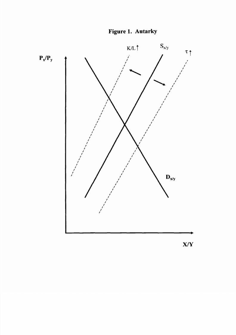
The relative demand and supply curves for lY are sketched in Figure

1.

Although t is an endogenous variable, equation (11) is nevertheless useful to help

build our intuition about the patterns of trade. Let us first suppose that pollution taxes are

identical across countries, but that one country (North) is more capital abundant. Since

capital is used

in the Y industry, this reduces the relative supply

of

X in the North,

shifting in the relative supply curve and pushing up the autarky relative prices of X

North has a comparative advantage in Y, and the pattern of trade will be determined by

factor endowment ratios: the capital abundant country exports the capital intensive good.

This is the standard Heckscher-Ohlin story.

If instead factor abundance ratios are identical across countries, but North has a

higher pollution tax, then since X is relatively clean, North s relative supply for X will

shift out to the right, generating a comparative advantage in X based on differences in

pollution policy. For identical factor endowment ratios, the country with stricter

pollut ion policy exports the clean good. Since from (5), pollution policy is determined by

income, then the trade pattern in this case is determined by income levels: North exports

7



the clean good and South exports the dirty good. This was the trade pattern in our earlier

papers (Copeland and Taylor

1994, 1995).

In the present paper, we assume that North is both capital abundant and rich.

Capital abundance shifts the relative supply curve in to the left, while high income shifts

the curve out and to the right. North s comparative advantage will be determined by the

relative strength

of

these two effects.

o

obtain a condition on pollution taxes that

determines the pattern

of

trade, note that because relative demands are identical across

countries, North will export X if its relative supply curve is to the right of South s. Using

(11)

and its Southern analogue, we find that

lY > X*/y*

for given p if and only if

L

*1K*) 1-/3) 1-a)/ /3-a)

>

LIK

(12)

Recalling that /3

> a,

then

as

we discussed above, (12) implies that if factor endowment

ratios (LIK) are identical across countries, then North will always export X if it is richer

(since then

t > t*).

On the other hand, if the countries

do

not differ too much in

aggregate income, but if Home is sufficiently capital abundant, then Home may import X

and export the pollution intensive good, despite its higher pollution tax. This is because

the price of Y depends on both the pollution tax

t ,

and on the cost of capital. A low

capital cost may more than offset high pollution taxes and result in North being an

exporter of the pollution intensive good.

Equation

(12)

tells only part

of

the story about the pattern

of

trade because

pollution taxes are endogenous. Let

us

now determine the equilibrium conditions for

free trade.

t

is useful to write these in terms

of

production shares. Let 8 px/l denote

the share

of

x production in national income. The for any p, we have from

(7):

Zx

= apx = apx a8

t yl

y

(13)

Similarly,

3 ,--1_-

8- -)

Zy

=

y

(14)

8



In autarky, the share

of

spending on x is the same as the share

of

x output in

national income, and hence 8

a

=

b. Once a country is opened up to trade, 8 and b may

differ. Because the share

of

world spending on X is given by b we must always have

p(x + x*)

=b,

p(x + x*) + (y+y*)

or

8q> + 8*(1 - »

=

b,

where q> 11 1+1*) is North s share

of

world income and 0

<

q>

<

1. Thus in free trade, if

production patterns differ across countries, b must lie between 8 and 8*. Consequently,

trade will typically cause 8 to rise in one country and fall

in

the other. Moreover, note

that if 8

>

8*, then Home must export X, because preferences are identical and

homothetic.

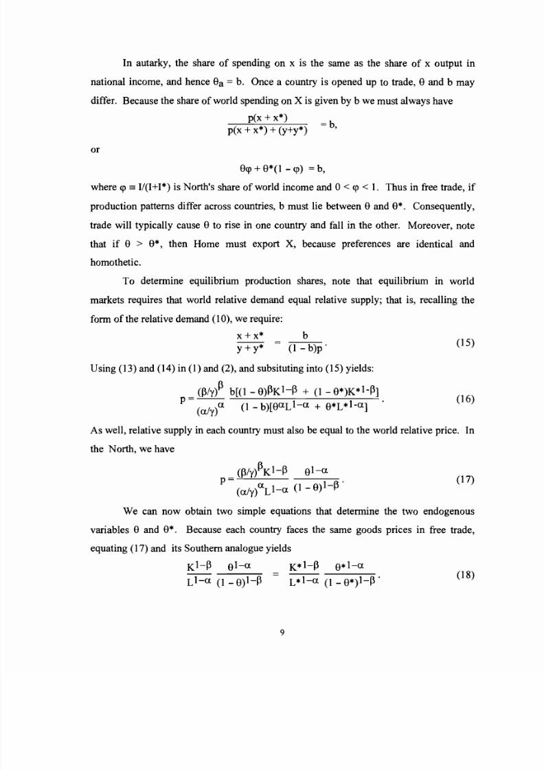
To determine equilibrium production shares, note that equilibrium in world

markets requires that world relative demand equal relative supply; that is, recalling the

form

of

the relative demand (10), we require:

x + x*

b

+y*

l b)p·

Using (13) and (14)

in

I) and (2), and subsituting into (15) yields:

(P/y)p b[(1 -

8)PKI-p

+

I

-

8*)K*I-p]

P

= u/y)u I - b)[8

U

LI-u

+

8*L*I-u]

(15)

(16)

As

well, relative supply in each country must also be equal to the world relative price. In

the North, we have

(17)

We

can

now

obtain two simple equations that determine the two endogenous

variables 8 and 8*. Because each country faces the same goods prices in free trade,

equating (17) and its Southern analogue yields

KI-P 8

1

-

u

K*I-P 8*I-u

=

LI-u I - 8)I-p

L*I-u 1- 8*)I-p·

(18)

9



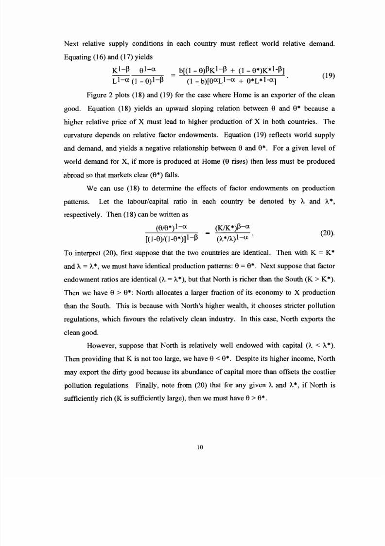
Next relative supply conditions in each country must reflect world relative demand.

Equating (16) and (17) yields

KI-P

8

1

-

a

Ll-a

1

- 8)I-p

b[(1 - 8)PKl-p 1 - 8*)K*I-p]

1 - b)[8

a

Ll-a 8*L*I-a]

(19)

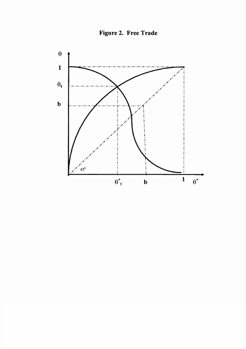
Figure 2 plots (18) and (19) for the case where Home is an exporter

of

the clean

good. Equation (18) yields an upward sloping relation between 8 and 8* because a

higher relative price of X must lead to higher production of X in both countries. The

curvature depends on relative factor endowments. Equation (19) reflects world supply

and demand, and yields a negative relationship between 8 and 8*. For a given level of

world demand for X, if more is produced at Home (8 rises) then less must be produced

abroad so that markets clear (8*) falls.

We can use (18) to determine the effects

of

factor endowments on production

patterns. Let the labour/capital ratio in each country be denoted by A and A*,

respectively. Then (18) can be written as

8/8*)I-a

[(1-8)/(1-8*)]

I-P

KIK*)p-a

( A*/ A)I-a .

(20).

To interpret (20), first suppose that the two countries are identical. Then with K = K*

and A = A*, we must have identical production patterns: 8 = 8*. Next suppose that factor

endowment ratios are identical

( A

=

A

*), but that North is richer than the South (K

>

K*).

Then we have 8

>

8*: North allocates a larger fraction of its economy to X production

than the South. This is because with North s higher wealth, it chooses stricter pollution

regulations, which favours the relatively clean industry. n this case, North exports the

clean good.

However, suppose that North is relatively well endowed with capital

( A

<

A

*).

Then providing that K is not too large, we have 8 < 8*. Despite its higher income, North

may export the dirty good because its abundance

of

capital more than offsets the costlier

pollution regulations. Finally, note from (20) that for any given A and A*, if North is

sufficiently rich (K is sufficiently large), then we must have 8 > 8*.

1



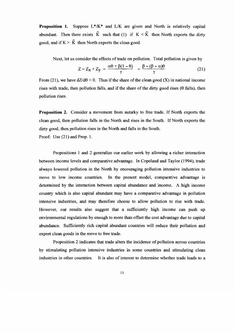
Proposition 1

Suppose L /K and LlK are given and North is relatively capital

- -

abundant. Then there exists K such that

1)

if K

<

K then North exports the dirty

good, and

if

K

>

K then North exports the clean good.

Next, let us consider the effects

of

trade on pollution. Total pollution

is

given by

a8

P 1

-

8)

P - P - a 8

Z = Zx Zy = Y = Y

21)

From 21), we have dZ/d8 < O Thus if the share of the clean good X) in national income

rises with trade, then pollution falls, and if the share of the dirty good rises 8 falls), then

pollution rises.

Proposition

2. Consider a movement from autarky to free trade.

If

North exports the

clean good, then pollution falls in the North and rises in the South.

If

North exports the

dirty good, then pollution rises in the North and falls in the South.

Proof: Use 21) and Prop.

1.

Propositions 1 and 2 generalize our earlier work by allowing a richer interaction

between income levels and comparative advantage. In Copeland and Taylor

1994),

trade

always lowered pollution in the North by encouraging pollution intensive industries to

move to low income countries. In the present model, comparative advantage is

determined by the interaction between capital abundance and income. A high income

country which is also capital abundant may have a comparative advantage in pollution

intensive industries, and may therefore choose to allow pollution to rise with trade.

However, our results also suggest that a sufficiently high income can push up

environmental regulations by enough to more than offset the cost advantage due to capital

abundance. Sufficiently rich capital abundant countries will reduce their pollution and

export clean goods in the move to free trade.

Proposition 2 indicates that trade alters the incidence of pollution across countries

by stimulating pollution intensive industries in some countries and stimulating clean

industries in other countries.

t is

also

of

interest to determine whether trade leads to a

11



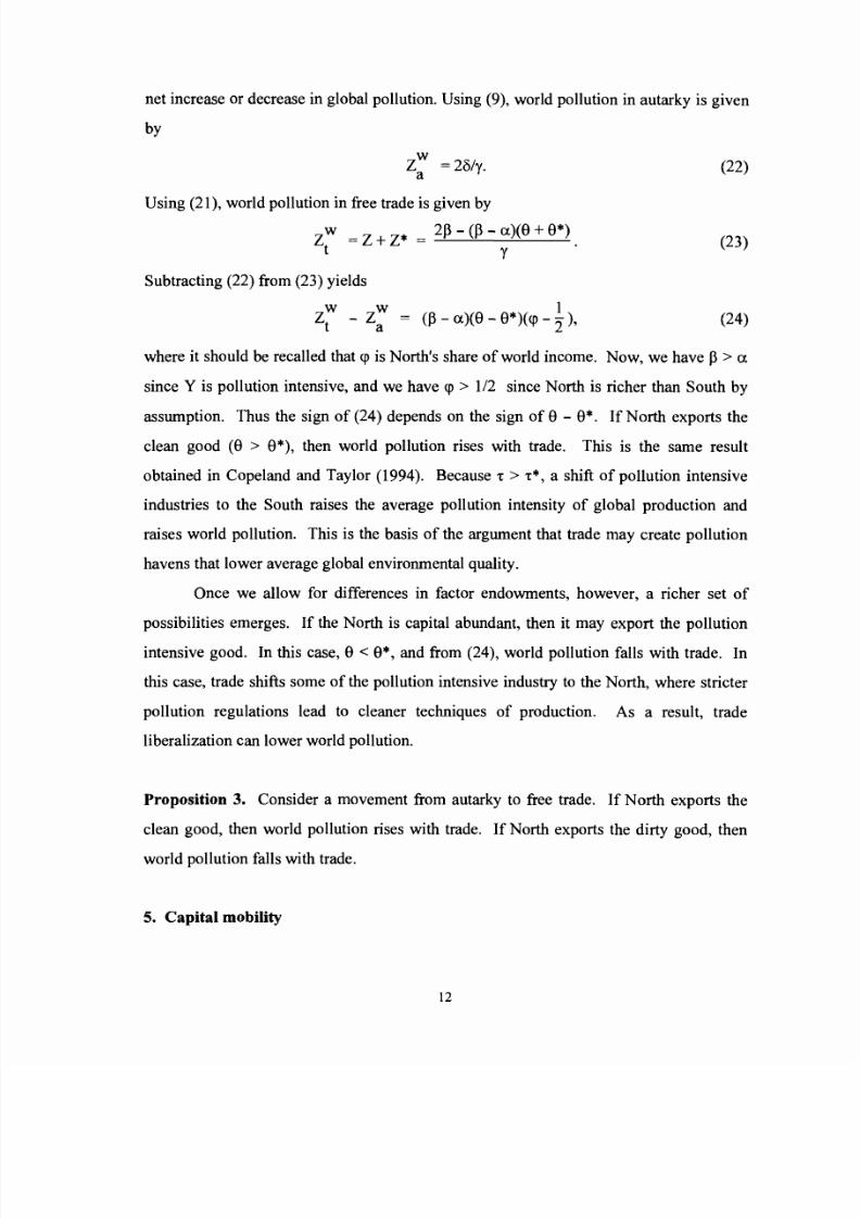
net increase or decrease in global pollution. Using (9), world pollution in autarky is given

by

w

Z = 23/y

a

Using (21), world pollution in free trade is given by

w

Z

= Z+Z*

t

Subtracting (22) from (23) yields

2/3 -

/3

- a)(8

8*)

y

w w

1

Zt

-

Za = (/3-a)(8-8*)(<p-2 ) '

(22)

(23)

(24)

where it should be recalled that

p

is North s share

of

world income. Now, we have 3

> a

since Y is pollution intensive, and we have p > 112 since North is richer than South by

assumption. Thus the sign

of

(24)

depends on the sign

of

8 - 8*.

If

North exports the

clean good

(8 > 8*),

then world pollution rises with trade. This is the same result

obtained in Copeland and Taylor (1994). Because

't

> t*, a shift

of

pollution intensive

industries to the South raises the average pollution intensity

of

global production and

raises world pollution. This is the basis of the argument that trade may create pollution

havens that lower average global environmental qUality.

Once we allow for differences in factor endowments, however, a richer set

of

possibilities emerges.

If

the North is capital abundant, then it may export the pollution

intensive good. In this case,

8 <

8*, and from

(24),

world pollution falls with trade.

In

this case, trade shifts some

of

the pollution intensive industry to the North, where stricter

pollution regulations lead to cleaner techniques

of

production. As a result, trade

liberalization can lower world pollution.

Proposition 3. Consider a movement from autarky to free trade. If North exports the

clean good, then world pollution rises with trade.

If

North exports the dirty good, then

world pollution falls with trade.

5. apital mobility

12





Comparing 26) with 22), we see that world pollution with both free trade and

mobile capital is the same as autarky world pollution. Since we have already compared

free trade pollution levels with autarky pollution levels in Proposition 3 it is

straightforward to determine the effects

of

capital mobility on world pollution.

Proposition 4. Consider a world that initially has free trade in goods, but not factors.

Now suppose that capital is allowed to flow freely between countries, and suppose that

both industries remain active in each country. Then a)

if

North initially exports the

clean good, world pollution will fall when capital is allowed to move; and b)

if

North

initially exports the dirty good, then world pollution will rise when capital is allowed to

move.

6. onclusion

In our earlier work, we developed a model in which countries differed only in

income levels. The purpose

of

that work was to isolate the role

of

income effects and

identify the influences that differences in income might have on the polluting effects

of

trade. In reality, trade is determined by the complex interaction

of

many different forces.

In this paper, we illustrate the interaction between the effects of factor endowment

differences with income effects.

Our results depend on the relative strength

of

the two forces.

f

income effects

dominate, then the results are much the same as before: trade can lead to the creation

of

pollution havens in poor countries and trade can increase world pollution. However,

if

differences in factor endowment ratios dominate, then richer countries may be net

exporters

of

pollution intensive goods and trade may reduce world pollution.

Capital mobility may raise or lower world pollution. However, in the case where

North initially exports the pollution intensive good, increased capital mobility may raise

world pollution from its free trade level. Since this case seems to be empirically relevant

during the development process, the concerns about the environmental effects

of

capital

14



mobility expressed by Daly and Goodland 1994) and others should be given close

scutiny.

t

should be noted however that free trade plus capital mobility leave world

pollution unchanged from its autarky level.

5



P

y

Figure 1 utarky

lLi

Sxly

X Y



igure

2

ree Trade

1

,-..0.;,,;'

=--

- , - , - , - , - , - , - , - , - , - , - , - , - , - ,

-:..:':;,-.-'

_ - ~

, ,

1

.

b

1

.f'

.

b

1

e



eferences

Copeland, B.R. and M.S. Taylor, North-South Trade and the Environment,

Quarterly

Journal

o

Economics

109 (1994): 755-87.

Copeland, B.R. and M.S. Taylor, Trade and Transboundary Pollution, American

Economic Review

85

(1995a): 716-737.

Daly, H. and

R

Goodland, An ecological-economic assessment

of

deregulation

of

international commerce under GATT,

Population and Environment 15

(1994): 395-

427.

Grossman, Gene M. and Krueger, Alan B., Environmental Impacts of a North American

Free Trade Agreement. in Peter Garber, ed.,

he Mexico-US. Free Trade

Agreement.

Cambridge, Mass.: MIT Press, 1993.

Low, Patrick, and Alexander Yeats, Do 'Dirty' Industries Migrate? in Patrick Low, ed.,

International Trade and the Environment: World Bank Discussion Papers

(Washington, DC: World Bank, 1992).

Rauscher, M., National environmental policies and the effects of economic integration,

European Journal o Political Economy

7 (1991): 313-29.

Richelle, Y.,

Trade

Incidence

on

Transboundary Pollution: Free Trade can Benefit the

Global Environmental Quality University

of

Laval Discussion Paper No. 9616

(1996).

6

Documents

A Simple Model of Trade_ Capital Mobility_ and the Environment