1

A SIMPLE SPEADSHEET MODEL TO INCORPORATE

SEASONAL GROWTH INTO LENGTH-BASED STOCK

ASSESSMENT METHODS

Gertjan de Graaf, Nefisco foundation, Lijnbaansgracht 14 C, 1015 GN Amsterdam,

the Netherlands, degraaf@nefico.org, www.nefisco.org

Pieter Dekker, Xi Consultancy, P.O. Box 1000, 2600 BA Delft, the Netherlands,

Dekker@Xi-advies.nl, www.xi-advies.nl

ABSTRACT

The paper describes a method by which seasonal growth can be incorporated in

length-converted catch curves and cohort analysis using a spreadsheet to carry out

the analysis. The method is based on calculating the length of fish with the seasonal

growth parameters on a daily basis after which a LOOKUP function is used to find

length and its corresponding age.

INTRODUCTION

The last decade, fisheries biologists working in tropical waters became increasingly

familiar with “length-based fish stock assessment”, mainly due to the development of

easy-to-use software, such as LFSA, ELEFAN, FISAT, and LFDA; and good training

manuals (Sparre and Venema, 1992); the worldwide FAO/DANIDA training course in

Tropical Fish Stock Assessment; and the availability of relatively cheap computers.

Most of the traditional stock assessment methods work with age composition data,

whereby “annuli” (on otoliths, scales and other bones) are used to estimate growth.

However, in tropical waters this type of “age reading” is almost impossible, and stock

assessment took off with the development of “length-based” methods.

2

In principle, “length-based fish stock assessment” is based on the conversion of

length into age, whereby in most cases it is assumed that the fish is growing

according to the von Bertalanffy Growth Function (VBGF). It is generally accepted

that in temperate waters, the growth of fish displays strong seasonal oscillations,

mainly due to fluctuations of temperature and/or food supply (Shul’man 1974).

However, strong seasonal growth exists in the tropics (Daget and Ecoutin 1976, de

Graaf and Ofori-Danson 1997, de Graaf, 2003). The need to use a seasonal version

of the VBGF has been discussed extensively by several authors (Pauly and Ingles

1981; Pauly et al., 1992, Longhurst and Pauly 1987; Sparre, 1990) and seasonal

versions of standard analytical models such as the ”yield per recruit” method

(Sparre, 1991) and length-converted catch curves (Pauly 1990) were developed and

incorporated in the different software packages. However, these models can be

considered as the basics of stock assessment providing a first idea on the status of

the stocks and the impact of fishing mortality. More detailed information, needed for

the formulation of fisheries management strategies, is provided through Virtual

Population Analysis (VPA) or length-based cohort analysis and Thompson and Bell

models (Sparre and Venema, 1992). Pauly et al. (1987) used the seasonal version of

the VBGF to slice the cohorts, in a time-based VPA for Peruvian Anchoveta, and this

techniques has been incorporated in the DOS version of FISAT, but the length-based

VPA in FISAT is still non -seasonal.

Therefore, if you want to analyse data yourself, in a spreadsheet, in most cases you

are depending on the mathematics of a non-seasonal model, with distorted results if

the growth is seasonal. In this paper, an approach is presented in which seasonal

growth can be incorporated in some major fish stock assessment methods using a

spreadsheet for analysis.

NON SEASONAL AND SEASONAL GROWTH

The basic tool for length-based methods is the conversion of “length-based data” into

“age-based data”. For the conversion of length into age in length-based fish stock

assessment, traditionally the VBGF is used. The non-seasonal version of VBGF

takes the form:

( )( )t

K tL L e t= −

∞

− −*

*1 0

3

Where

Lt Length at time t

Loo L infinitive or asymptotic length

K growth parameter

to T zero, or time when the fish are born or entered in the system

The growth rate at any point in the lifespan of the fish can be calculated with:

( )tLLKdtdL

−= ∞

Conversion of length into age is being done with the inverse VBGF:

( )

−−=

∞LL

KtLt o 1ln

1

In conclusion, the conversion of length-based data into age-based data for non-

seasonal growth is rather straightforward. However, this is not the case with seasonal

growth. The seasonal version of the VBGF (Somers, 1988) has the following form:

( ) ( ) ( ){ }e soso ttðttððCKttKLtL

)](2sin)(2[sin2/1

−−−−−−∞ −=

Where:

Lt Length at time t

L∞ L infinitive

K growth rate parameter

t0 T-zero

ts the onset of the first oscillation relative to t=0, or ts = Winter point + 0.5”

C the intensity of the (sinusoid) growth oscillations

The parameter C is important as it determines the intensity of the seasonal growth.

When C=0, seasonal growth is absent and the equation equals the standard VBGF.

At C=1, growth comes to a standstill once a year at the winter-point. Intermediate

values of C indicate growth reduction during the winter, but growth never completely

stops.

4

0

2

4

6

8

10

12

14

0 0.5 1 1.5 2 2.5

Age (year)

Len

gth

(cm

)

024681012141618

dL

/dt

(cm

/yea

r)

Length dL/dt

0

2

4

6

8

10

12

14

0 0.5 1 1.5 2 2.5

Age (year)

Len

gth

(cm

)

0

5

10

15

20

25

30

35

dL

/dt

(cm

/yea

r)

Length dL/dt

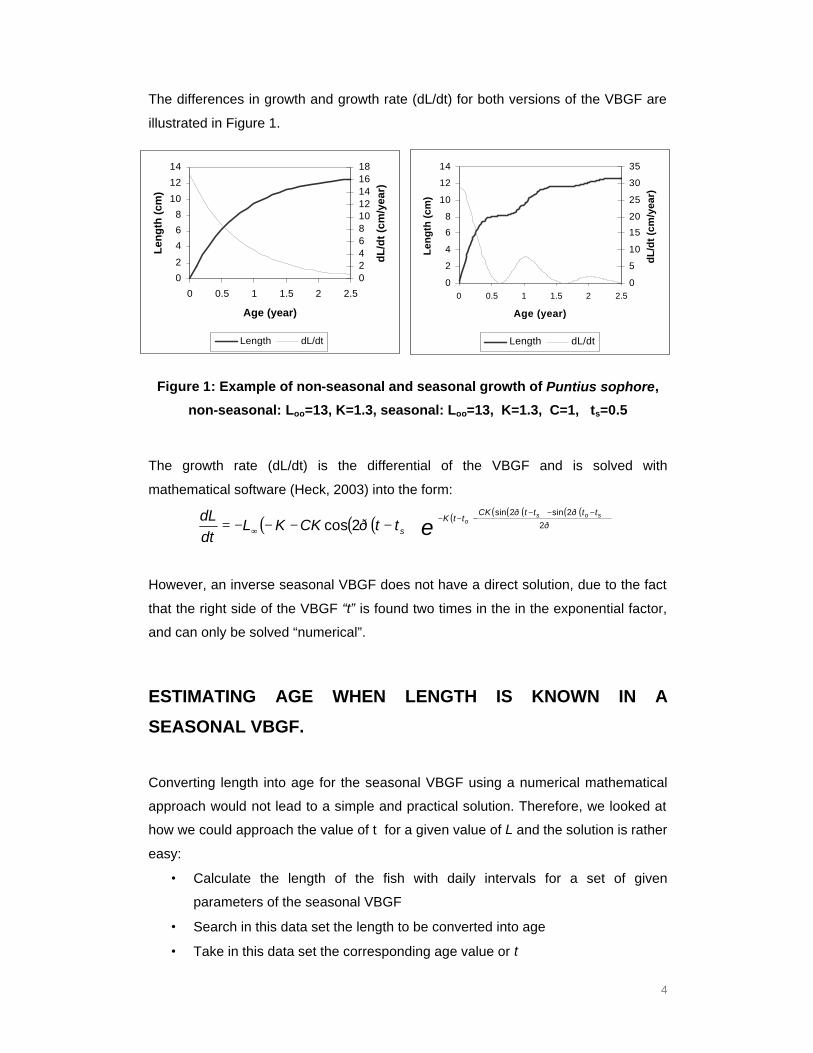
The differences in growth and growth rate (dL/dt) for both versions of the VBGF are

illustrated in Figure 1.

Figure 1: Example of non-seasonal and seasonal growth of Puntius sophore,

non-seasonal: Loo=13, K=1.3, seasonal: Loo=13, K=1.3, C=1, ts=0.5

The growth rate (dL/dt) is the differential of the VBGF and is solved with

mathematical software (Heck, 2003) into the form:

( )( )( ) ( ) ( )( ) ( )( )( )

e ð

ttðttðCKttK

s

sosottðCKKL

dtdL

−−−−−−

∞ −−−−= 2

2sin2sin

2cos

However, an inverse seasonal VBGF does not have a direct solution, due to the fact

that the right side of the VBGF “t” is found two times in the in the exponential factor,

and can only be solved “numerical”.

ESTIMATING AGE WHEN LENGTH IS KNOWN IN A

SEASONAL VBGF.

Converting length into age for the seasonal VBGF using a numerical mathematical

approach would not lead to a simple and practical solution. Therefore, we looked at

how we could approach the value of t for a given value of L and the solution is rather

easy:

• Calculate the length of the fish with daily intervals for a set of given

parameters of the seasonal VBGF

• Search in this data set the length to be converted into age

• Take in this data set the corresponding age value or t

5

In a spreadsheet, this can be done with a “LOOKUP” function, as explained below.

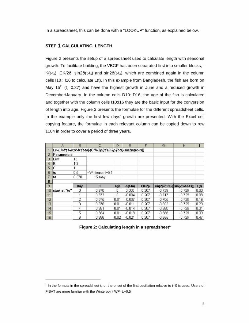
STEP 1 CALCULATING LENGTH

Figure 2 presents the setup of a spreadsheet used to calculate length with seasonal

growth. To facilitate building, the VBGF has been separated first into smaller blocks; -

K(t-to); CK/2ð; sin2ð(t-ts) and sin2ð(t-to), which are combined again in the column

cells I10 : I16 to calculate L(t). In this example from Bangladesh, the fish are born on

May 15th (to=0.37) and have the highest growth in June and a reduced growth in

December/January. In the column cells D10: D16, the age of the fish is calculated

and together with the column cells I10:I16 they are the basic input for the conversion

of length into age. Figure 3 presents the formulae for the different spreadsheet cells.

In the example only the first few days’ growth are presented. With the Excel cell

copying feature, the formulae in each relevant column can be copied down to row

1104 in order to cover a period of three years.

Figure 2: Calculating length in a spreadsheet1

1 In the formula in the spreadsheet ts or the onset of the first oscillation relative to t=0 is used. Users of

FISAT are more familiar with the Winterpoint WP=ts+0.5

6

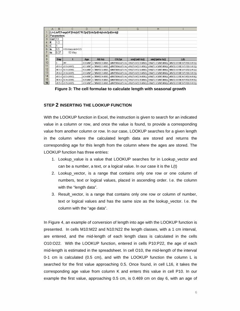
Figure 3: The cell formulae to calculate length with seasonal growth

STEP 2 INSERTING THE LOOKUP FUNCTION

With the LOOKUP function in Excel, the instruction is given to search for an indicated

value in a column or row, and once the value is found, to provide a corresponding

value from another column or row. In our case, LOOKUP searches for a given length

in the column where the calculated length data are stored and returns the

corresponding age for this length from the column where the ages are stored. The

LOOKUP function has three entries:

1. Lookup_value is a value that LOOKUP searches for in Lookup_vector and

can be a number, a text, or a logical value. In our case it is the L(t)

2. Lookup_vector, is a range that contains only one row or one column of

numbers, text or logical values, placed in ascending order. I.e. the column

with the “length data”.

3. Result_vector, is a range that contains only one row or column of number,

text or logical values and has the same size as the lookup_vector. I.e. the

column with the “age data”.

In Figure 4, an example of conversion of length into age with the LOOKUP function is

presented. In cells M10:M22 and N10:N22 the length classes, with a 1 cm interval,

are entered, and the mid-length of each length class is calculated in the cells

O10:O22. With the LOOKUP function, entered in cells P10:P22, the age of each

mid-length is estimated in the spreadsheet. In cell O10, the mid-length of the interval

0-1 cm is calculated (0.5 cm), and with the LOOKUP function the column L is

searched for the first value approaching 0.5. Once found, in cell L16, it takes the

corresponding age value from column K and enters this value in cell P10. In our

example the first value, approaching 0.5 cm, is 0.469 cm on day 6, with an age of

7

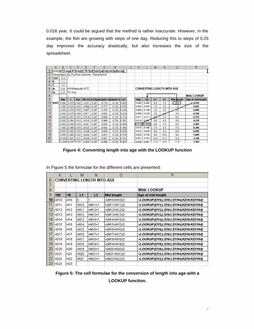
0.016 year. It could be argued that the method is rather inaccurate. However, in the

example, the fish are growing with steps of one day. Reducing this to steps of 0.25

day improves the accuracy drastically, but also increases the size of the

spreadsheet.

Figure 4: Converting length into age with the LOOKUP function

In Figure 5 the formulae for the different cells are presented:

Figure 5: The cell formulae for the conversion of length into age with a

LOOKUP function.

8

Length-based methods are often used when length composition data for the total

fishery is available for a one-year period only. This is often the case in fish stock

assessment programmes in developing countries where the funds for continuous

fishery monitoring are lacking. Catch curves and cohort analysis can be applied

under these conditions as their basic assumption is the constant parameter system:

The picture presented by all length classes caught during one year reflects that of a

single cohort during its entire life span (Sparre and Venema, 1992). In the next

paragraphs it will be demonstrated how our method can be used for the construction

of a linearized length-converted catch curve and cohort analysis when growth is

seasonal.

LINEARIZED LENGTH-CONVERTED CATCH CURVE

The construction of a catch curve is the most common approach to estimate the total

mortality of a cohort. Details behind the method are well presented by Sparre and

Venema (1992) and Gayanilo and Pauly (1997) and are only briefly summarized

here. Assuming constant recruitment and constant mortality the length converted

catch curves takes the form:

'ln ii

i ZtadtC

+=

Where

C catch number of length class i

dti time needed of the fish to grow through length class i

Z Total mortality

ti’ age of the mid-length of length class i

a constant

For non-seasonal growth dti is estimated from

( )

−

−=

∞

+∞

i

ii LL

LLKdt 1ln1

and ti’ is estimated from

( )

−=

∞LL

Kt ii 1ln1'

9

Sparre (1990) and Pauly (1990) clearly demonstrated that the total mortality is

overestimated with a traditional catch curve, if seasonal growth is not accounted for.

The reason is that dti and ti’ depend not only on length but also on the time of the

year if growth is seasonal. Pauly (1990) developed a method using the parameters

of the seasonal VBGF to identify a number of pseudo cohorts to resolve this problem,

which is incorporated in FISAT. It is rather complicated to apply this method in a

spreadsheet; therefore, we explain how a catch curve can be made with the

LOOKUP function, providing results comparable with the method of Pauly. We

illustrate this with an example of Puntius sophore from Bangladesh.

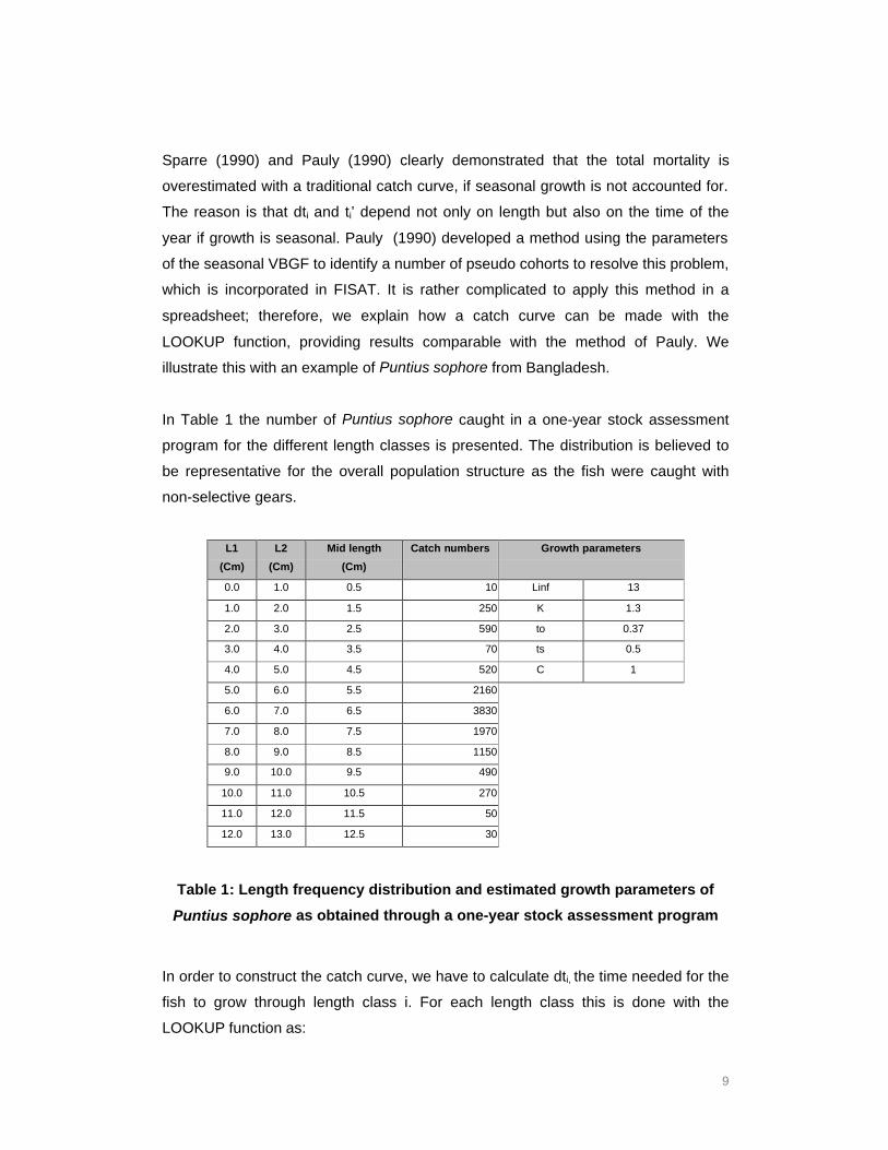
In Table 1 the number of Puntius sophore caught in a one-year stock assessment

program for the different length classes is presented. The distribution is believed to

be representative for the overall population structure as the fish were caught with

non-selective gears.

L1

(Cm)

L2

(Cm)

Mid length

(Cm)

Catch numbers

Growth parameters

0.0 1.0 0.5 10 Linf 13

1.0 2.0 1.5 250 K 1.3

2.0 3.0 2.5 590 to 0.37

3.0 4.0 3.5 70 ts 0.5

4.0 5.0 4.5 520 C 1

5.0 6.0 5.5 2160

6.0 7.0 6.5 3830

7.0 8.0 7.5 1970

8.0 9.0 8.5 1150

9.0 10.0 9.5 490

10.0 11.0 10.5 270

11.0 12.0 11.5 50

12.0 13.0 12.5 30

Table 1: Length frequency distribution and estimated growth parameters of

Puntius sophore as obtained through a one-year stock assessment program

In order to construct the catch curve, we have to calculate dti, the time needed for the

fish to grow through length class i. For each length class this is done with the

LOOKUP function as:

10

dt =age L2-age L1

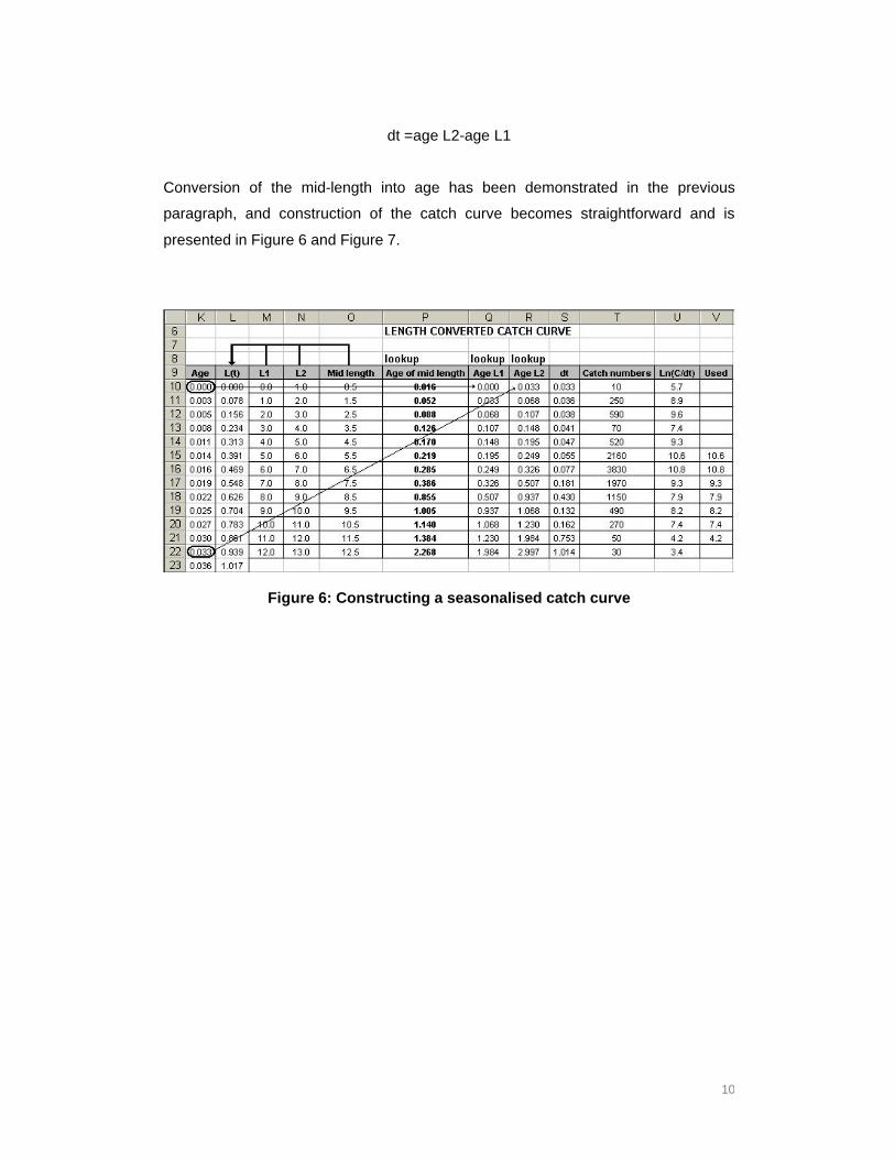
Conversion of the mid-length into age has been demonstrated in the previous

paragraph, and construction of the catch curve becomes straightforward and is

presented in Figure 6 and Figure 7.

Figure 6: Constructing a seasonalised catch curve

11

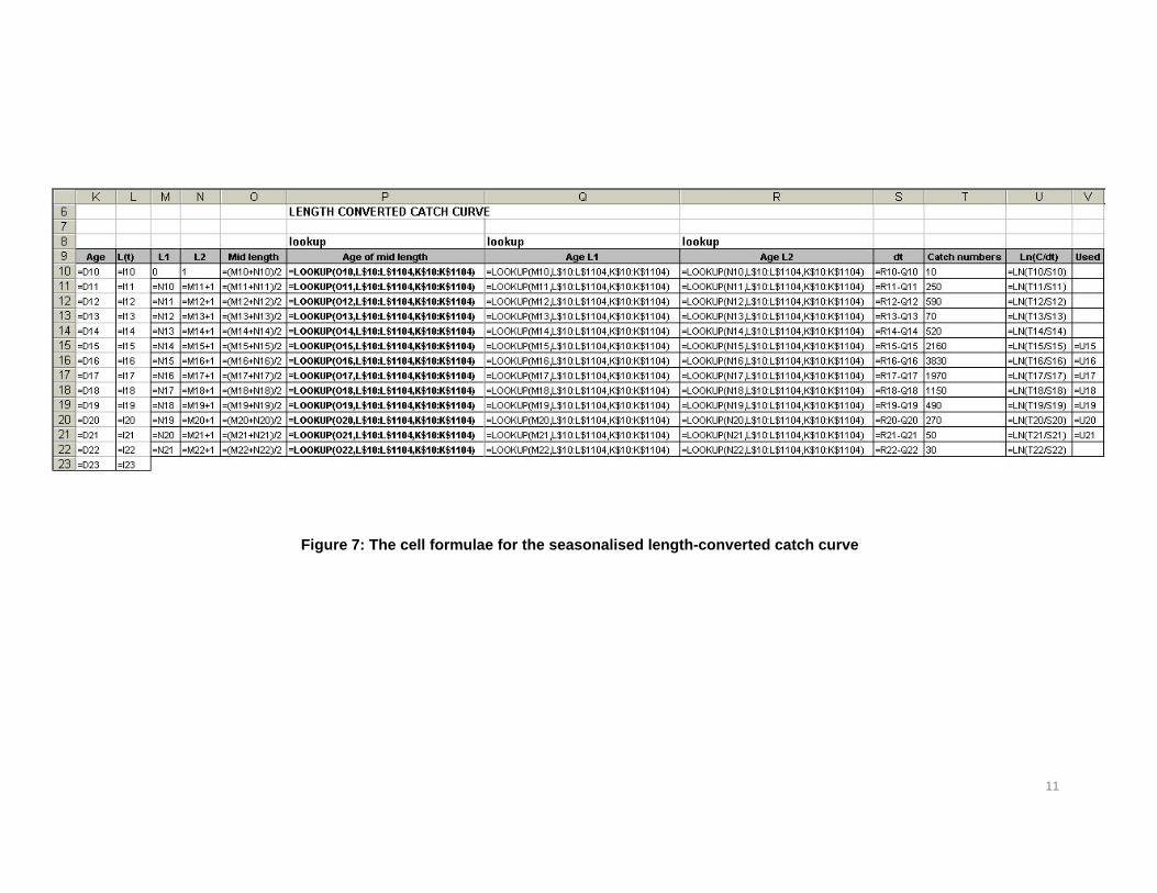
Figure 7: The cell formulae for the seasonalised length-converted catch curve

12

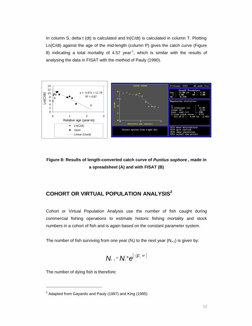
In column S, delta t (dt) is calculated and ln(C/dt) is calculated in column T. Plotting

Ln(C/dt) against the age of the mid-length (column P) gives the catch curve (Figure

8) indicating a total mortality of 4.57 year-1, which is similar with the results of

analysing the data in FISAT with the method of Pauly (1990).

Figure 8: Results of length-converted catch curve of Puntius sophore , made in

a spreadsheet (A) and with FISAT (B)

COHORT OR VIRTUAL POPULATION ANALYSIS2

Cohort or Virtual Population Analysis use the number of fish caught during

commercial fishing operations to estimate historic fishing mortality and stock

numbers in a cohort of fish and is again based on the constant parameter system.

The number of fish surviving from one year (Nt) to the next year (Nt+1) is given by:

( )[ ]t t

MN N e tF+

− +=1

*

The number of dying fish is therefore:

2 Adapted from Gayanilo and Pauly (1997) and King (1995)

y = -4.57x + 11.79R2 = 0.87

02468

101214

0 1 2 3

Relative age (year-to)

Ln(C

/dt)

Ln(C/dt)

Used

Linear (Used)

13

( )t

Z

N e* 1− −

The catch (Ct) is the proportion dying owing to fishing, and may be estimated from

the catch or Baranov (1926) equation;

( )[ ]( )tt

t

F MC F N eZ=

− − +* * 1

Combining the different equations will give the Gulland (1965) equation for Virtual

Population Analysis:

( )t

t

t

t

CN

FZ e tZ

+

=

−1

1*

Given values of the catch (Ct), and an estimate of the natural mortality M, the

equation can be used to estimate retroactively the size of the past cohorts, if an

estimate of Nt+1 is available from which to start the computation. Estimates of Nt+1

(expressing the last population size a cohort had before it became extinct) are called

“terminal population” Nt. Values of Nt can be obtained from:

t tt

tN Z C

F= *

Where Ct, is the terminal catch (i.e. the last catch taken from a cohort before it went

extinct) and Ft is the terminal fishing mortality, i.e. the fishing pressure that generated

Ct. A VPA starts with an initial guess of Ft and then calculates backwards with the

known catches and natural mortality rate (Figure 9):

14

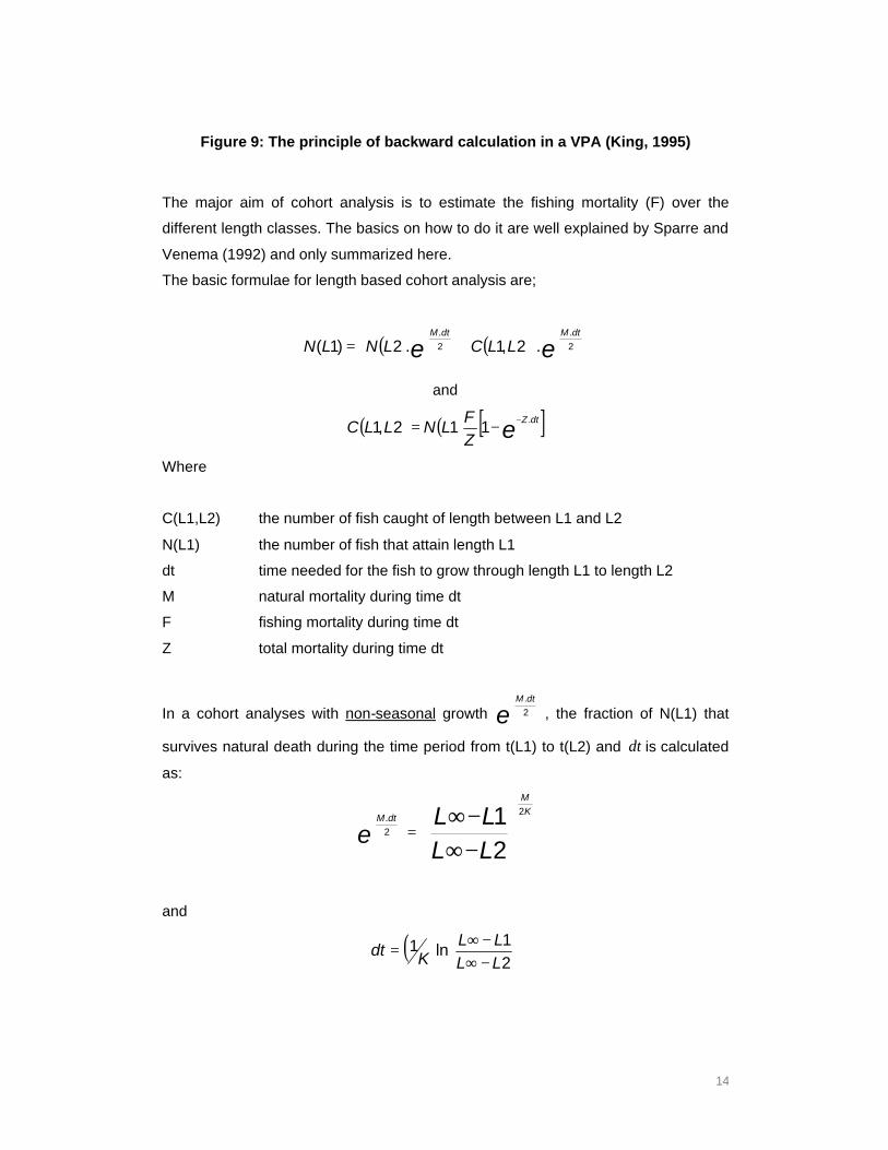
Figure 9: The principle of backward calculation in a VPA (King, 1995)

The major aim of cohort analysis is to estimate the fishing mortality (F) over the

different length classes. The basics on how to do it are well explained by Sparre and

Venema (1992) and only summarized here.

The basic formulae for length based cohort analysis are;

( ) ( ) eedtMdtM

LLCLNLN

+= 2

.

2

.

.2,1.2)1(

and

( ) ( ) [ ]edtZ

ZF

LNLLC.

112,1−−=

Where

C(L1,L2) the number of fish caught of length between L1 and L2

N(L1) the number of fish that attain length L1

dt time needed for the fish to grow through length L1 to length L2

M natural mortality during time dt

F fishing mortality during time dt

Z total mortality during time dt

In a cohort analyses with non-seasonal growth edtM

2

.

, the fraction of N(L1) that

survives natural death during the time period from t(L1) to t(L2) and dt is calculated

as:

−∞−∞

=

21 2

2.

LLLL

eK

M

dtM

and

( )

−∞−∞

=21

ln1LLLL

Kdt

15

Again with seasonal growth the last formulae will give incorrect results. However, dt

can be calculated as: dt =age L2-age L1, which can be solved with the LOOKUP

function and thus we can use the basic formulae edtM

2

.

directly.

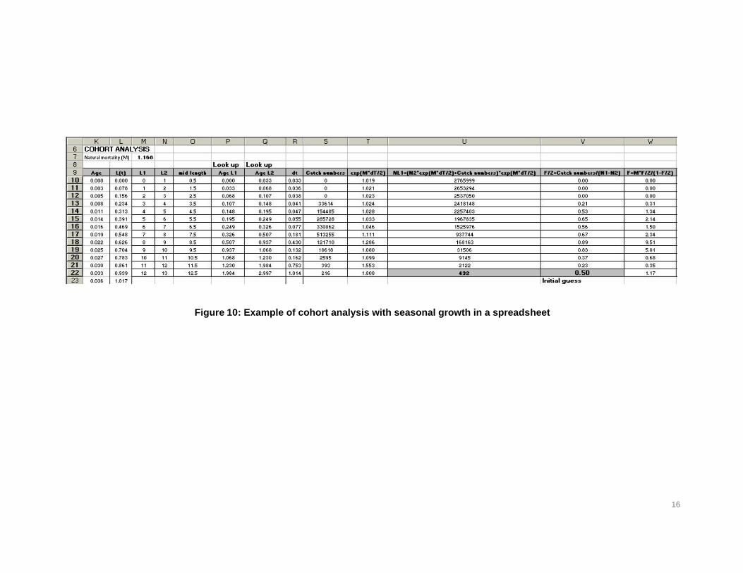
In Figure 10 an example of a cohort analysis in a spreadsheet for Puntius sophore

with a natural mortality of M=1.168 year-1 (all other parameters are the same as

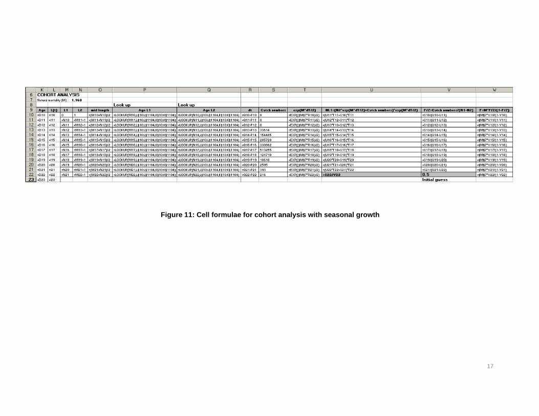
those in the previous examples) is presented; the cell formulae are presented in

Figure 11.

16

Figure 10: Example of cohort analysis with seasonal growth in a spreadsheet

17

Figure 11: Cell formulae for cohort analysis with seasonal growth

18

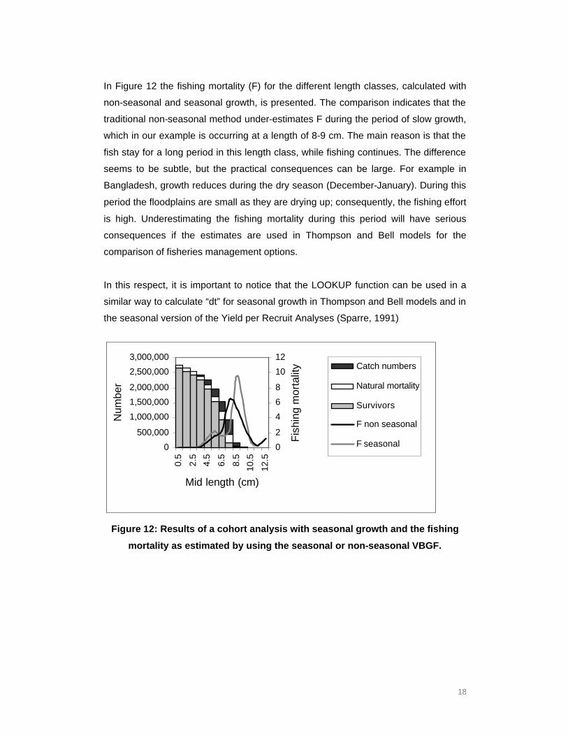
In Figure 12 the fishing mortality (F) for the different length classes, calculated with

non-seasonal and seasonal growth, is presented. The comparison indicates that the

traditional non-seasonal method under-estimates F during the period of slow growth,

which in our example is occurring at a length of 8-9 cm. The main reason is that the

fish stay for a long period in this length class, while fishing continues. The difference

seems to be subtle, but the practical consequences can be large. For example in

Bangladesh, growth reduces during the dry season (December-January). During this

period the floodplains are small as they are drying up; consequently, the fishing effort

is high. Underestimating the fishing mortality during this period will have serious

consequences if the estimates are used in Thompson and Bell models for the

comparison of fisheries management options.

In this respect, it is important to notice that the LOOKUP function can be used in a

similar way to calculate “dt” for seasonal growth in Thompson and Bell models and in

the seasonal version of the Yield per Recruit Analyses (Sparre, 1991)

Figure 12: Results of a cohort analysis with seasonal growth and the fishing

mortality as estimated by using the seasonal or non-seasonal VBGF.

0

500,000

1,000,000

1,500,000

2,000,000

2,500,000

3,000,000

0.5

2.5

4.5

6.5

8.5

10.5

12.5

Mid length (cm)

Num

ber

0

2

4

6

8

10

12

Fis

hing

mor

talit

y Catch numbers

Natural mortality

Survivors

F non seasonal

F seasonal

19

LIMITATION OF THE PROPOSED METHOD

The proposed method provides convenient results but has some limitations. First of

all, the time of recruitment should be known. This is a minor limitation as in most

cases it is known during which month major spawning takes place.

Secondly, the used seasonal version of the VBGF of Somers (1988) has exactly one

zero growth rate per year when C=1, which means that for each length there will

always be one value for its age. Using this version of the VBGF will do for most

tropical fisheries, where prolonged periods of zero growth will be an exception. The

method cannot be applied if the seasonal version of the VBGF of Pauly et al (1992) is

used as this version allows for longer periods of “no growth”, which means that a

length can have several values for age, i.e. we cannot convert length into age.

A similar problem arises if there are two cohorts per year, which is often the case in

penaeid shrimps. Then again, there is no “one-to-one” correspondence between age

and length (Sparre 1990). In this case, the only solution is to slice the cohorts (Sparre

and Venema, 1998) and apply a VPA with pseudo cohorts (Pauly et al. 1987,

Gayanilo and Pauly, 1997)

THE SPREADSHEETS

The different spreadsheets can be downloaded from our website

www.nefisco.org/Training.htm

AKNOWLEDGEMENTS

We would like to thank Mr. Jordi Lleonart (FAO, Rome, Italy) and Mr Daniel Pauly

(University of British Colombia, Vancouver, Canada) for their useful comments on the

first version of the manuscript and of course Tracy Barnett for the nice editing of the

document.

20

REFERENCES

Baranov, F.I. (1926)_ On the question of the dynamics of the fishing industry.

Naunchn Byull. Rybn. Khoz. 8 (1925), 7-11 (in Russian)

Daget , J. and Ecoutin, J.M. (1976) Modeles mathematiques de production

applicables aux poissons tropicaux subissant un arret annuel prolonge de

croissance. Cahiers ORSTOM, serie hydrobiologie 10 (2), 59-69.

de Graaf, G.J. & Ofori-Danson P.K. (1997) Catch and fish stock assessment in

stratum VII of Lake Volta. IDAF Technical Report/97/1, GHA/93/008. Rome: FAO,

107 pp.

de Graaf, G.J. (2003) The floodpulse and growth of floodplain fish in Bangladesh.

Fisheries Management and Ecology (10), 241-247.

Gayanilo, F.C. and Pauly, D. (1997) FAO-ICLARM stock assessment tools (FISAT),

reference manual. FAO computerized information series (Fisheries). No. 8, Rome,

FAO, 262 p.

Gulland, J.A. (1965) Estimation of mortality rates. Annex to Artic fisheries working

group report ICES C.M. 1965/D:3, (Reprinted as pp 231-241 in P.H. Cushing (ed),

Key papers on fish populations. IRL Press, Oxford, 1983)

Heck, A. (2003) Introduction to Maple 3rd Edition. Springer-Verlag, New York, 844 pp

Longhurst, A.R. and Pauly, D. (1987 Ecology of tropical oceans. Academic Press,

San Diego, California. 407 p.

Pauly, D. (1990) Length converted catch curves and the seasonal growth of fishes.

ICLARM Fishbyte 8 (3), 33-38.

21

Pauly, D. and Ingles, J. (1981) Aspects of growth and natural mortality of exploited

coral reef fishes. In: E. Gomez, C.E. Birkeland, R.W. Buddemeyer, R.E. Johannes,

J.A. Marsh, Jr. and R.T. Tsuda (eds), Proceedings of the Fourth International Coral

Reef Symposium, Manila, Philippines, Vol. 1, pp 89-98.

Pauly, D., Palomares, M.L. and Gayanilo, F.C. (1987) VPA estimates of monthly

population length composition, recruitment, mortality, biomoass and related statistics

of Peruvian Anchoveta, 1953 to 1981. In D. Pauly and I. Tsukayama (eds), ICLARM

Stud REV . 15, pp 142-166.

Pauly, D., Soriano-Bartz, M., Moreau, J. and Jarre Teichman, A. (1992) A new model

accounting for seasonal cessation of growth in fishes. Australian Journal Marine and

Freshwater Research. 43, pp 1151-1156.

Shul’man G.E. (1974) Life cycles of fish: Physiology and biochemistry. Wiley and

Sons, New York. 257 pp.

Somers I.F. (1988) On a seasonal oscillating growth function. ICLARM Fishbyte 6

(1), 8-11.

Sparre, P. and Venema, S.C. 1992. Introduction to tropical fish stock assessment,

Part 1-manual. FAO Fisheries technical paper 306-1 rev. 1. 376 p.

Sparre, P. and Venema, S.C. (1998) Introduction to tropical fish stock assessment,

Part 1-manual. FAO Fisheries technical paper 306-1 rev. 2. 385 p.

Sparre, P. (1990) Can we use traditional length-based fish stock assessment when

growth is seasonal. Fishbyte pp 29-32.

Sparre, P. (1991) Estimation of yield per recruit when growth and fishing mortality

oscillate seasonally. Fishbyte pp 40-44.