A Simple, Systematic Method for Determining J Levels for jj Coupling Ensign Steven J. Gauerke, USN, and Mark L. Campbell United States Naval Academy, Annapolis, MD 21402-5026

The accurate description of atomic structure relies heav- ily on the coupling of angular momenta in the valence elec- trons of the atom. Such coupling is normally described in two limiting representations: LS or jj coupling. At the un- dergraduate level the student is usually taught only RussellSaunders, or LS, coupling. Indeed, current text- books in physical (1) and inorganic (2) chemistry discuss the Russell-Saunders case almost exclusively. The book by Atkins (la) does attempt to handle the jj-coupled case for the p2configuration but does so incorrectly.

A predominant reason for the neglect textbook authors have shown for jj coupling is the perceived difficulty in finding the terms and levels associated with this scheme. In this Journal, Ruhio and Perez (3) describe a method that they proclaim as simple. Unfortunately, their method is difficult to follow, and its proper use is not obvious except with the simplest electron configurations. The only other method we have found in the literature was described by Tuttle (4). Again, this treatment is more complicated than is desirable for instruction at the undergraduate level. In this paper, we describe a process that is based on the same concepts as Thttle's but is simpler and more systematic, allowing for application a t the undergraduate level.

Angular Momentum Coupling In LS coupling, the valence electrons'individual orhital

angular momenta e's couple to yield the total orhital angu- lar momentum L, which is a constant of the motion. In terms of the classical model of the precession of vectors, this means that the Y's precess more rapidly around their mutual field than around any other field. Similarly, the in- dividual spins s's couple to yield the total spin angular mo- mentum S, which is also a constant of the motion.

States represented by a particular combination of L and S are called a term. The determination of LS term symbols for different electron configurations has been covered ex- tensively in this Journal (5-7). In general, several LS terms will result from any one electron configuration.

For each term the spin-orbit interaction is treated as a small perturbation yielding a representation in which the total electronic angular momentum J of the atom is the vector sum of the orbital and spin angular momenta. Its quantum numbers cover a range.

L+S,L+S-1, ... I L - S I The result is that each term is split into levels that consist of states with the same value of J that are (21 + 1)-fold degenerate corresponding to the possible values of MJ.

Limitations of L S Coupling

LS wupling is an appropriate description when the non- central electrostatic energy t e r n for the valence electrons are much larger than the spin-orbit terms. The electro- static interaction normally predominates in ground-state electronic configurations for light to moderately heavy at- oms. However, in ground configurations of heavy atoms and in many excited configurations of light and heavy at- oms, the spin-orbit energy of the valence electrons contrib-

utes to a larger fraction of the energy perturbation than the residual electrostatic energy.

LS wupling inadequately describes the observed states in these cases. The levels given by ji coupling may then be used to explain the absences of multiplets predicted by LS coupling, as well as the presence of LS-forbidden transi- tions that are allowed by jj-coupling selection rules.

J Coupling a s the Preferred Scheme

In cases where jj wupling is the more appropriate cou- pling scheme, the electrons appear to move independently of one another and in these circumstances the individual values j, t , and s are the good quantum numbers. Each electron's t and s couple to give j, the electron's total angu- lar momentum. As with LS coupling, several terms result from the different ways in which each electron can couple its angular momenta.

For each term the electrostatic interaction is treated as a small perturbation yielding a representation in which the total electronic angular momentum J of the atom is the vector sum of each electron's angular momentum.

The result is that each term is split into levels, which again consist of states with the same value of J that are (21 + 1)-fold degenerate. Due to a correlation of states, for a given electron configuration one finds the same J levels in jj coupling as in LS coupling although there are gener- ally many more terms with the LS coupling case (except in the case of p" and s" configurations).

Preferred Notation

Although the notation used for LS coupling is univer- sally standardized, the notation for jj coupling is not. For jj-coupled terms, we prefer the notation

where 1 and 1' are the letter designations for the type of orbitals (i.e., s, p, d, etc.), and e, e' are the numerical values of the angular momentum quantum numbers for the elec- trons.

In the other common notation system (3,4,8) the terms are designated solely by thej's,

which obscures important information needed to deter- mine allowed spectral transitions between jj-coupled states. As an illustration of the ambiguity that may result consider the forbidden transition

which is incorrectly characterized in ref 8 as an allowed transition. Using the notation

Volume 71 Number6 June 1994 457

one might erroneously conclude that this is an allowed transition based on j-coupling selection rules (9). How- ever, with the preferred notation, it is apparent that the transition is forbidden because this transition requires that two electrons change their quantum numbers.

iidoupled States for an In Configuration .. - The method for determiningj-coupled states presented

in this section is based on the application of the Pauli ex- clusion principle in governing-the possible microstates that compose an electron configuration. A microstate is a articular auantum state in which each electron in the atom is associated with a set of unique quantum numbers. The Pauli exclusion ~ r i n c i ~ l e is most often intemreted in terms of the strong held case in which the e's i d s's for each electron are uncoupled from each other, so they are all space-quantized with good quantum numbers me and m,.

Use of the mj Representation

However, the weak field case, in which an individual electron's t and s couple to give j and its space quantization m, is the more appropriate representation when discussing jj coupling. The Pauli exclusion principle still applies in this case: No two electrons within the atom can have the same complete set (n, e, s, j, m,) of quantum numbers. Be- cause the spin quantum number for an electron has the value V2. the ~ossible values of i for anv eiven electron can only be ln'and t - 112. for an"2ectron configura- tion of the t m 1" there will be a t most two tvoes of elec- trons. ~ a c L of these forms a subset of equrGalent elec- trons--equivalent electrons being defined as having the same value of n, e, s, and j.

According to the exclusion principle, for each subset of equivalent electrons, only those microstates in which the mj values are different will be allowed. The following method allows the determination ofjj-coupled states by de- termining all possible combinations of m:s for each subset ofequivaient electrons and then using cokelation of states to detfrmme the allowed J states for a given term.

Determining Energy Levels and Possible n r m s Energy levels forj-coupled terms can be determined by

canying out the following procedure.

Stepl.

Step 2.

Step 3.

Step 4.

Step 5.

Step 6.

Determine the possible %-coupled terms for the given electron configuration.

For each term found above. set uo a table of all ~~~ ~ ~

possible combinations of mjva~uds for the term consistent with the Pauli exclusion principle and the indistinguishability of electrons.

Determine the value of MJ(= Em,) for each microstate (row) in the table.

Determ ne tne maxlmum value of M ~ f r o m tne values in the MJ colmn. Tne argea va ue of M~represents a value of Jforthat term.

Eliminate the 2J+ 1 values of MJ (J, J - I , J+1,-J)

that comprise the J state determined in step 4.

Repeat steps 4 and 5 until all Mjvalues are eliminated for the term.

According to our procedure, the fnst step in determining the allowed J levels is to derive the possible terms for the configuration. The jj-coupled terms for an electron configu- ration in which only one subshell is partially filled will have the form

where n represents the number of electrons in the partially fdled subshell, and the value of i is constrained such that

n Z i Z 0 far suhshells less than half-filled 2e Z i Z 0 far half-filled subshells 2e Z i Z n - 2e - 2 for subshells more than half-filled

The number of terms will be

n + 1 for subshelk less than half-filled n for half-filled subshells 4e + 3 - n for subshells mare than half-filled

Once the terms have been determined, construct a mi- crostate table in which each allowed microstate appears once and only once. Microstates that are simple permuta- tions of the same m, values within each subset of equiva- lent electrons do not represent different states. Thus, only one of these microstates should be included in the table. We have found a systematic way to set up this table.

Const~cting the Microstate Table

Subsets for Equivalent Electrons

Construct a table with n + 2 columns. In the fnst row of the table, label the first n columns with the j states of the electrons in which the smaller values of j are placed to the left. In the second row, label the first n columns with mj; (i = 1 to n) to indicate the allowed magnetic quantum num- bers for each electron. Equivalent electrons are grouped. (In our tables, we use double lines to designate the group- ing of equivalent electrons.)

within each subset of equivalent electrons, treat the m, values as runnineindices: the values of mi to the rieht varv faster than those to i t s left. ~ imi lar l i , each sibset o"f equivalent electrons is treated as a running index with the subset to the right as the faster changing index. Once an m, value is changed in the group of equivalent electrons to the left, all the possible combinations of mj values for the subset to the right are determined for that one combina- tion.

To initiate the construction of the table, set up the first row of numerical values for mj in the table so that the val- ues of mj are maximized. Accomplish this by setting the value of m, a t the far left of each subset of equivalent elec- trons with the maximum mj possible, that is, the numeri- cal value ofj. The succeeding values of m, to its right de- crease by 1 sequentially. Fill out succeeding rows by treating each column of m, values as running indices as described previously.

Checks for the Table

When this process is carried out correctly, all the values of mj in a particular row for a subset of equivalent elec- trons are different, and the mj values will decrease from left to right. As a check, if a value of mj in a particular row in a subset of equivalent electrons has a value greater than or equal to another m, value to its left, then the table has been filled out incorrectlv.

Once the table is mmpleted, check to be sure that all pos- sible cornhinations have been determined. The nurnher of microstates for a particular term of the form

is given by the product of the binomial coefficients for each subset of equivalent electrons.

458 Journal of Chemical Education

Table 1. Microstate Tables for a p3 Configuration

Tables 1 and 2 illustrate the construction of microstate tables for the terms for the p3 and p4 electron conflgura- tions. In each subset of equivalent electrons, the m, values always decrease from left to right. Furthermore, within each subset of equivalent electrons, the mj value to the right varies the fastest, followed by the one to its left, and so forth.

Using MJ Values To Determine the J Level

After constructing the microstate table and determining the MJ values for each microstate, the J levels are deter- mined according to steps 4 and 5. Onee a J level is deter- mined from the maximum MJ value in the table, then the (W + 1) MJ values associated with that J level are elimi- nated.

For example, in Table 1 for the term [(p*)'(p3,&, the maximum MJ value is 312, which results in a J value for this term of 3/2. As step 5 is carried out, all four MJ states 312, 112, -112, and -312 are eliminated. Because there are no MJ states remaining, the only level for this term is the 3/2 level.

From the microstate table for the [(pm)'(pm)'1 term in Table 1, the maximum value of MJ is 512. Thus, a J level for this term is 5/2. and the M.7 states 512. 312. 112. -112. -3/2. . . . and 6/2 are elkinated, asrndicated with an asterisk next to these values. After eliminating the six microstates asso- ciated with the J = 5/2 level, thi maximum MJ value re- maining is 3/2, yielding a J level for this term of 3/2. Elimi- nating the four microstates for this level, indicated with a @ in the table, leaves a maximum MJ value of ID. Thus, the final level for this t e rn is 1/2.

Table 2. Microstate Table for a p4 Configuration

As in this case, when more than one microstate has the same value of MJ, the question arises Which of the MJ's should be eliminated for a specific value of J?" The short answer is "It doesn't matter as long as the student elimi- nates one and only one of the microstates (rows) for each of the corresponding (W+ 1) MJ values for the given J."

Obviously, this method can become quite laborious for electron configurations with more than a few electrons. For example, the term consists of 90 micro- states and 14 J levels. Because constructing such a table is time-consuming and tedious, we have included Table 3 which gives all the possible J levels for terms that arise from s", p", d", and f" electron configurations. The electron configurations in Table 3 are .grouped in complementary pairs; the same J levels occur for configurations of the form 1" and 1"' where n'= 48 + 2 - n.

It helps students to construct tables for a few simple cases but not tables consist in^ of hundreds of microstates. Nonetheless, students benefitfr~munderstandin~ how the levels for the more complex cases are determined even if they do not determine the levels themselves.

Computer Programming The systematic nature of this method allows easy appli-

cation to computer programming. Acopy of the FORTRAN program used to generate Table 3 can be obtained by writ- ing M. Campbell. The program consists of less than 100 lines of com~uter code and uses a series of nested DO loo~s and IF stat;rnents to determine the possible microstatks for the inputted term. The values of M., are calculated and tabulated for each microstate, and then steps 4 and 5 of our procedure are applied until all the microstates have been taken into account.

jjGoupled States for I" I " Configurations Table 3 can also be used to determine jj-coupled states

for electron configurations in which more than one sub- shell is partially filled. In some cases, jj-coupled terms can

Volume 71 Number 6 June 1994 459

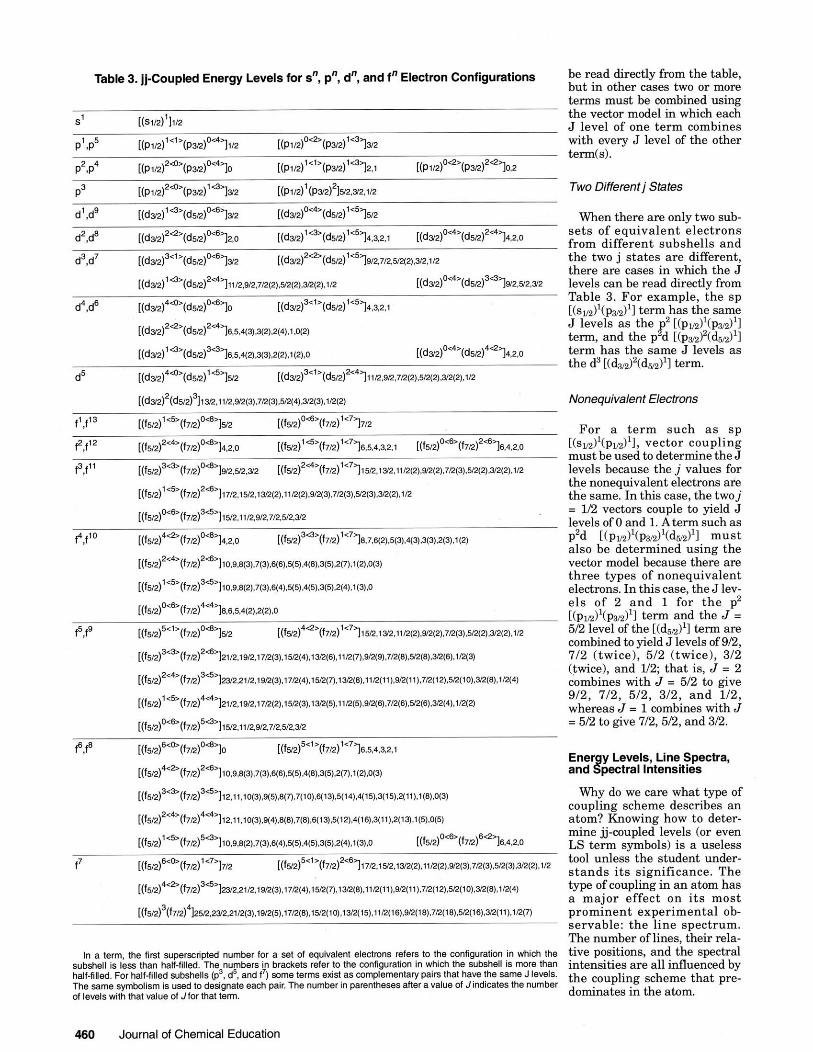
Table 3. jj-Coupled Energy Levels for sn, p", dn, and f" Electron Configurations be read directly from the table, but in other cases two or more terms must be combined using the vector model in which each J level of one term combines with every J level of the other term(s).

Two Differentj States

When there are only two sub- sets of equivalent electrons from different subshells and the two j states are different, there are cases in which the J levels can be read directly from Table 3. For example, the sp [(sm)'(pm)'l term has the same J levels as the p2 Kpm)l(pgJ11 term, and the p d [(~m)~(dsn)'l term has the same J levels as the d3 [(d3n)2(dm)'l term.

Nonequivalent Electrons

For a term such a s sp [ ( S ~ ~ ) ~ ( ~ ~ ) ' I , vector coupling must be used to determine the J levels because the j values for the nonequivalent electrons are the same. In this case, the twoi

[(15n)~'~(hrz)~~'115n,11~912~7/2,512.312 = 1/2 vectors couple to yield J levels of 0 and 1. A term such as

f4,fi0 [(f5i2)4*(h~)0"'~4,2,0 1(f~2)~~'(f712)"~~8,7,6(2),5(3),q31,3(3),2(3),1(2) p2d [(pvz)'(p3iz)'(dm)'l must also be determined using the

[(fu~~2'4'(hn~2"'~lo,~,e~3~.7(3),7(3),4~8l.3~5~~2~7).1~2~.~~3~ vector model because there are three types of nonequivalent

[(fu2)1'~(f7n)36'l1o,~,8(2),7(3~,6(4),5(~).4(5),~(5).2(4).5 electrons. In this case. the J lev- ~ ~~ ~

[(fsn)0'~(hn)4"'la,665,4~2),2~2),~ els of 2 and 1 for t he p2 [(pm)'(p3,)'1 term and the J =

f5,f9 [(fs45"'(hn)0"'l~2 [(fs2)4Q'(f7~~)1'7~~u2,tm,~i~(2),9~2(2),7~(3),w2(2)~2(2), i~2 512 level of the [(d5n)'l term are combined to yield J levels of 9/2,

[(f5~)3'b(b~)2"'~21~,19/2,17~(3),15n(4),1~(6),11~(7),912(9),712(8),u2(8),~(6),l~2~3) 712 (twice), 512 (twice), 312 (twice), and V2; that is, J = 2

[(fw2)2c"(f~n)36'~~,21i2,19~(3),17n(4),1~p),1m(8),lln(tl),9n(ll),7n(12),u2(lo),~(8),ln(4~ combines with J = 512 to give

[(fsn)1'5'(f7n)4"'l2t/~,t9~22i7n~2~,i~(3~,i3n~~~,iin~~~,~n~e~,7n~~~,vr~e~,m~~~,~rz~~~ 912, 712, 512, 312, and 112, whereas J = 1 combines with J

[(fsn)0'"(hrz)5Q'li~n,ii~~~227~12~~/2z2 = 512 to give 712, 512, and 312.

P f [(fsn)6'b(bn)0"'10 [(fsn)5"'(f7n)1'7~6,5,~43322i Ene y Levels, Line Spectra, [(fs12)4"2(~7~)2"'~10,9,6(3),7(3),~(6),5(5),4(6),3(5)~ and$ectral Intensities

[(fsn~3'3'(f7rz~3~'li~,tt1io~3~,~~5~,8~7~,7~i~),~~3),~~~4~,qi5~,~~i~~,~~ii~,~~e~,o~~~ Why do we care what type of coupling scheme describes an

~~sn)~'"(17~~~"'1i2,11,io~3~,~~4~,~~8~,7~e~,~~~~~,t,i~~,3~1i~,2~13~,1~~~,o(~1 atom? Knowing how to deter- mine jj-wupled levels (or even

[ ( f s z ) 1 ' 5 ' ( f 7 n ~ 5 o ' ~ t o , ~ 9 ~ ~ 2 ~ . 7 ~ ~ ~ , e ~ 4 ~ , ~ ~ ~ ~ , 4 ~ ~ ~ , ~ ~ 5 ~ , 2 ~ 4 ~ . t ~ 3 ~ . o [ ( 1 s n ) ~ ' ~ ( 1 7 ~ ) ~ ~ ' 1 ~ , 4 ~ 2 , 0 LS term symbols) is a useless

f7 [ ( f~n)~'~(b~)"~'17/~ [(1y~)~"'(f7~)~'~~17~,1~2,1~2(2),1ii2(2),~(3),7~(3),~2(3),312(2),1/2 tool unless the student under- s tands i ts significance. The

[ ( ~ s 1 ~ ) ~ < " ( 1 ~ n ~ ~ ~ ' 1 ~ ~ ~ e ~ ~ , 1 ~ n ~ ~ ~ , i ~ n ~ ~ ~ , i ~ ~ ~ , ~ m ~ ~ ~ , ~ ~ ~ ~ t ~ ~ , g n ~ i i ~ , ~ n ~ i ~ ~ , ~ ~ i o ~ , m ~ ~ ~ , ~ n ~ 4 ~ type of coupling in an atom has a major effect on i t s most

4 [(f5/~)~(17/2) 125~.2~2,21~(3) ,19~2(5) ,1712~8l ,15 /2~10l ,1z2(15) .11n(16) ,9~~16~,7~~18~.~~~16)11) .1~~) prominent experimental ob- servable: the line spectrum. The number of lines, their rela-

In a term, the lint superscripted number for a set of equivalent electmns refen to the mnfiguration in which the tive positions, and the spectral Subshell is less than half-filled. The numbers in brackets refer to the configuration in which the subshell is more than intensities me all influeneed by half-filled. For half-filled subshells (p3, d5, and f7) some terms exist as mmpiementary pain that have the same J levels. the coupling scheme that pre- The same symbolism is used to designate each pair The number in parentheses aner avalue of Jindicates the number of levels with that value of Jfor thatterm. dominates in the atom.

460 Journal of Chemical Education

However, for tellurium and polo- nium the two higher energy lev- els of the predicted triplet are very far removed from the ground state, so in these cases jj coupling is a better approxima- tion.

The Group 16 case is partieu- larly interesting due to the order of the lowest energy levels. Ac- cording to LS coupling, the ground-state triplet should con- sist of the J = 2 level as the low- est energy level, followed by the J = 1 and then the J = 0 level. This energy ordering is seen in oxygen, sulfur, and selenium. Ac- cording to jj coupling, the lowest term results in the J = 2 level be- ing the lowest energy level, with the J = 0 level being the next low- est. From the next term. the J = 1 level appears as the tdird low-

4 est enem. This enerm orderine -" - is foun$;n tellurium and polo-

Figure 1. Energy levels for the np4 electron configuration of the Group 16 elements. The experimental nium. The fact that the two cou- values tor the J levels were taken from ref 10. pling schemes correctly predict

the experimentally observed or-

4 Coupling as the Preferred Scheme: ncreasing Atomic Mass

der of energy levels for the Group 16 atoms is a rather remarkable accomplishment in the description of atomic structure.

Group 16 Elements Group 14 Elements It is interesting to compare the actual experimentally Another example of how3 coupling becomes more impor-

measured properties of atoms with those predict4 theo- tant as the atomic mass increases is illustrated in Fimrre retically by the different coupling cases. The energy levels 2, This figure shows the energy levels for the ground t&m for the p4 ground-state configuration for the Gmup 16 ele- and first excited terms of the Group 14 elements along ments are shown in F i r e 1 along with the predicted lev- with the levels predicted assuming LS and jj coupling. LS els for LS and jj coupling. coupling is a very accurate description for carbon, silicon,

From Figure 1 we see that the LS prediction is very good germanium, and tin, although the energy spacings in- for oxygen, sulfur, and selenium although the energy spac- crease as the atomic mass increases. However, for lead the ings in the triplet increase as the atomic mass increases. two higher energy levels of the triplet are very far removed

from the ground state, so jj cou- pling is a hetter approximation.

In the case of the n'snp excited state, LS coupling describes carbon and silicon very well. However, for germanium, tin, and lead the energy levels ap- pear more as two double-energy levels, a s predicted by jj cou- pling. These observations for the Group 14 elements are true in general. For ground-state elec- tron configurations very heavy elements follow jj coupling, whereas light to moderately heavy elements follow LS cou- pling. However, in excited-state configurations, jj coupling is often observed in lighter atoms.

Genera2 Appearance of the Spectrum

Another indication of which coupling scheme best describes an atom is the general appear- ance of the s~ectrum and the in-

Figure 2. Energy levels for the tp2 and n ' s ~ electron configurations of Ihe Group 14 elements. The tensity relations for the lines in experimental values for the J levels were taken from ref 10. the spectrum. As an example,

Volume 71 Number 6 June 1994 461

250 300 350 400 450 500 Wavelength (nm)

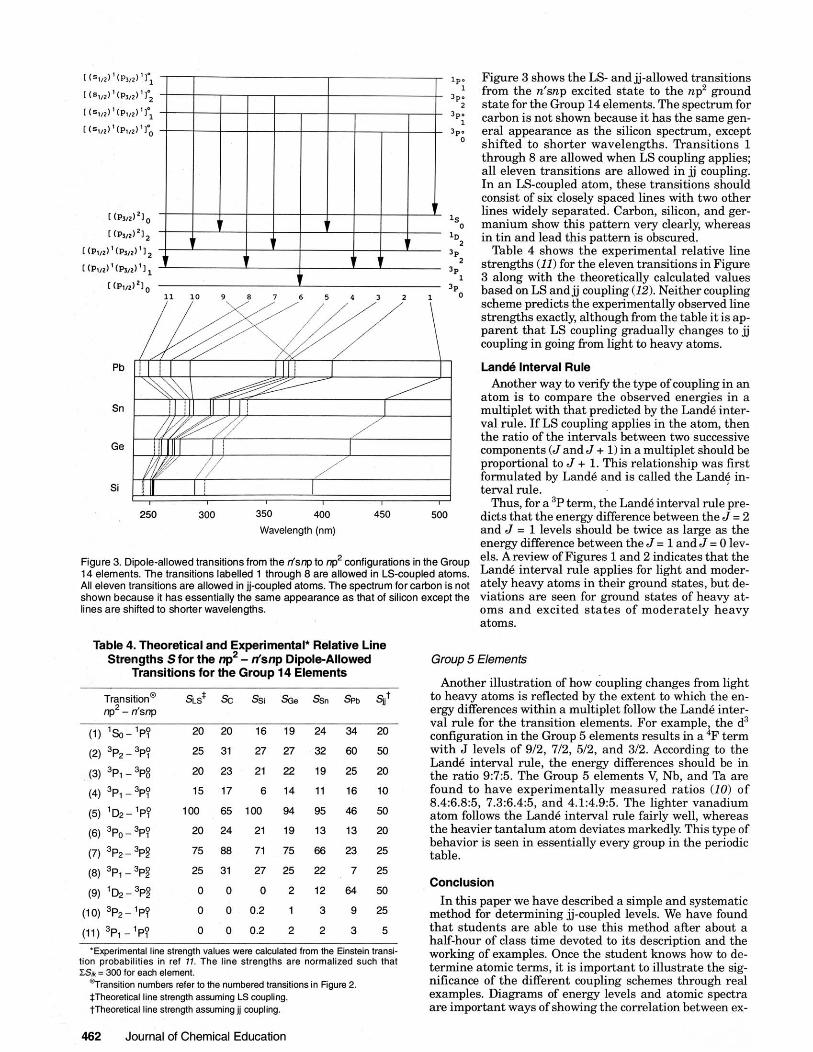
Figure 3. Dipole-allowed transitionsfrom the rlsnp to np2configurations in the Group 14 elements. The transitions labelled 1 throuoh 8 are allowed in LS-couoled atoms. All eleven transat ons are al owed in .lauplea-atoms The spectrum for camon is not shown oecaJse it has essenlla ly tne same appearance as !hat of sl lmn excepl the I nes are shlheo to shoner wave engths

Table 4. Theoretical and Experimental* Relative Line Strengths Sfor the np2 - n'snp DipoleAllowed

Transitions for the Group 14 Elements

rans sit ion^ 2

SLS* Sc Ssi So. Ssn S P ~ Sjjt np - n'snp

(1) 1 ~ - ' ~ 9 20 20 16 19 24 34 20

. . 'Elgwrimental line strength values were calculated hom the Einstein transi-

tion probab~lities in ref 11. The line strengths are normalized such that ZSx= 300 for each element.

%anransition numbers refer to the numbered transitions in Figure 2. *Theheoretical line strength assuming LSeaupling. tThwretical line strength assuming jj mupling.

Figure 3 shows the LS- andjj-allowed transitions from the n'snp excited state to the np2 ground state for the Group 14 elements. The spectrum for carbon is not shown because it has the same gen- eral appearance as the silicon spectrum, except shifted to shorter wavelengths. Transitions 1 through 8 are allowed when LS coupling applies; all eleven transitions are allowed in ji coupling. In an LS-coupled atom, these transitions should consist of six closely spaced lines with two other lines widely separated. Carbon, silicon, and ger- manium show this pattern very clearly, whereas in tin and lead this pattern is obscured.

Table 4 shows the experimental relative line strengths (11) for the eleven transitions in Figure 3 along with the theoretically calculated values based on LS andjj coupling (12). Neither coupling scheme predicts the experimentally obsewed line strengths exactly, although from the table it is ap- parent that LS coupling gradually changes to jj coupling in going from light to heavy atoms.

Lande Interval Rule Another way to verify the type of coupling in an

atom is to compare the obsewed energies in a multiplet with that predicted by the Land6 inter- val rule. If LS coupling applies in the atom, then the ratio of the intervals between two successive components (Jand J + 1) in a multiplet should be proportional to J + 1. This relationship was first formulated by Land4 and is called the Land$ in- terval rule.

Thus, for a 3P term, the Land6 interval rule pre- dicts that the energy difference between the J = 2 and J = 1 levels should be twice as large as the energy difference between the J = 1 and J = 0 lev- els. Areview of Figures 1 and 2 indicates that the Land6 interval rule applies for light and moder- ately heavy atoms in their ground states, but de- viations are seen for ground states of heavy at- oms and excited states of moderately heavy atoms.

Group 5 Elements

Another illustration of how doupling changes from light to heavy atoms is reflected by the extent to which the en- ergy differences within a multiplet follow the Land6 inter- val rule for the transition elements. For example, the d3 configuration in the Group 5 elements results in a 4F term with J levels of 912, 712, 512, and 312. According to the Land6 interval rule, the energy differences should be in the ratio 9:7:5. The Group 5 elements V, Nb, and Ta are found to have experimentally measured ratios (10) of 8.4:6.8:5. 7.3:6.4:5. and 4.1:4.9:5. The liehter vanadium atom follows the ~ h d 6 interval rule fa& well, whrrras the heavier tantalum atom deviates markedlv. This t w n of behavior is seen in essentially every group in the table.

Conclusion In this paper we have described a simple and systematic

method for determining jj-coupled levels. We have found that students are able to use this method aRer about a half-hour of class time devoted to its description and the working of examples. Once the student knows how to de- termine atomic terms, it is important to illustrate the sig- nificance of the different coupling schemes through real examples. Diagrams of energy levels and atomic spectra are important ways of showing the correlation between ex-

462 Journal of Chemical Education

perimentally determined energy states and theoretically D. coneisp ~~~~~~b chamisby, 4th 4.: chapman and H ~ I : N ~ W york, 1991: pp 940-950 (dl Huheey. J. E. Inorganic ChemiatryPrinc;ph ofStructuroandRmc.

derived states described by LS and jj coupling. It is also B V ~ ~ J . znd d.; H W ~ I and ow: N ~ W york, 1978; pp 810.814. (el meader. G. L.; useful for the student to understand that other relation- TW, D. A. ~norgonic chamisby; ~ r e n t i c e ~ d l : ~ n g ~ e w o o d GIG. NJ. 1991; pp

ships, such as spectral intensities and the Land6 interval 4248. lfl Owen. S. M.: Brooker, A. T A Gui& Lo M d m Inorganic Chemistry; W,ley:NewYork. 1991:pp 156160. (g! Shsrpe,A. G.InorganbChemidry.3rd ed.:

rule, can be used to verify the type of coupling that occurs wlley: NCW ymk. 1992; pp 7275.

in an atom. 3. Rubio. J.: Perel, J. J. J. Cham. Edue. 1986, 63,476. 4. lirtUe,R. R . A m r J.Phys. 1967.35.26.

Literature Cited 5. Cornan. M. J. Cham Ed-. 1973.50. 189. 6. Hyde, K.E. J C h r m E d u c 1915,52,87.

1. 1alAtkins.P WPhysimlChemisby, 5thed.;Freeman: NewYork, 1994: pp447-455. 7. Vi-te,J. J. Cham. Educ. 1989,60,561. ( b ! A l W , R. A.:Silky, R.J.Physlm1 Chemistry; W~ley: New Yark, 1992; pp37G 375. lcl Naggle, J. H. Physiml Chamisfry, 2nd 4.: Sldt, Foreman: Glenview, IL,

8. Richtmyer, F. K.; Kennard, E. H.; Cmper, J. N. Inlmduelion foM&rn Physics, 6th ed.: Mdjraw-Hill: New York, 1969: p 457.

1989;pp 712728.1d!Lwine,I.N.Phyaicol Chemishy:3dd.;McCraw-EI11: New York 1g88; pp 63M40, Berry, R, s,: S, A: Rosr, Physial

9. Leighton, R. B. fin=ipl= d M o d D m P h ~ i c s ; McCraw-Ell: New York, 1959: P 271.

mley:NewYork, 1980, pp 168.199. (0 Barmar, G. M. physieol chamisby, 5th ~d.; 10. Moore, C. E. Ammie Emrsy h o d s 1; NSRDS-NBS 35; U.S. Government %ting

MGraw-Hill: New York, 1988: pp4M65.1g)Dybtra. C. E. Quonhlm Chamlafry %ce Washinpton. DC. 1971; Vols. 1-3.

and M d a u l a r S p a t m o p y : Rentiee Hall: Englewood Cliffs, NJ, 1992; pp 2& 11. Wieae, W. lr: Martin, 0. A. Womlengfha and h s i t i o n Robabilities forAfrmsond 270. Afomlclons, Part 1I: NSRDS-NBS 68; U S Government Printing Ofice: Washing-

2. I a ) S h r i ~ e r , D . ~ ; A t h a , T ! W.;Langford,C.H.InowanieChsmislry:Freeman:New ton. DC, 1980. Yo* 1930; pp 434-41. lbl Butler I. 8.; H a d , J. F Inawanb Chemistry Pnnci- 12. Condon, E.U.; Shortleyi G. H. The TheoryofAttmiiSppef~; Ccbr idgeU~i i i i i I ty : ph8 andApplbztlons; BenjaminiCumminga: New York, 1999: pp 4245. IdLee, J. Cambridge, 1935: pp 247.285.

Volume 71 Number 6 June 1994 463