Chapter 1

A Simple Vision System

In 1966, Seymour Papert wrote a proposal for building a vision system as a summer project[Papert1966]. The abstract of the proposal starts stating a simple goal: “The summer visionproject is an attempt to use our summer workers effectively in the construction of a significantpart of a visual system”. The report then continues dividing all the tasks (most of which alsoare common parts of modern computer vision approaches) among a group of MIT students.This project was a reflection of the optimism existing on the early days of computer vision.However, the task proved to be harder than anybody expected.

The goal of this first chapter is to present several of the main topics that we will coverduring this course. We will do this in the framework of a real, although a bit artificial, visionproblem.

The goal of the rest of this chapter is to embrace the optimism of the 60’s and to buildan end-to-end visual system. During this process, we will cover some of the main conceptsthat will be developed in the rest of the course.

Vision has many different goals (object recognition, scene interpretation, 3d interpreta-tion, etc) but in this chapter we’re just focusing on the task of 3d interpretation.

1.1 A simple world: The blocks world

As the visual world is too complex, we will start by simplifying it enough that we will beable to build a simple visual system right away. This was the strategy used by some of thefirst scene interpretation systems. L. G. Roberts [Roberts1963] introduced the Block World,a world composed of simple 3D geometrical figures.

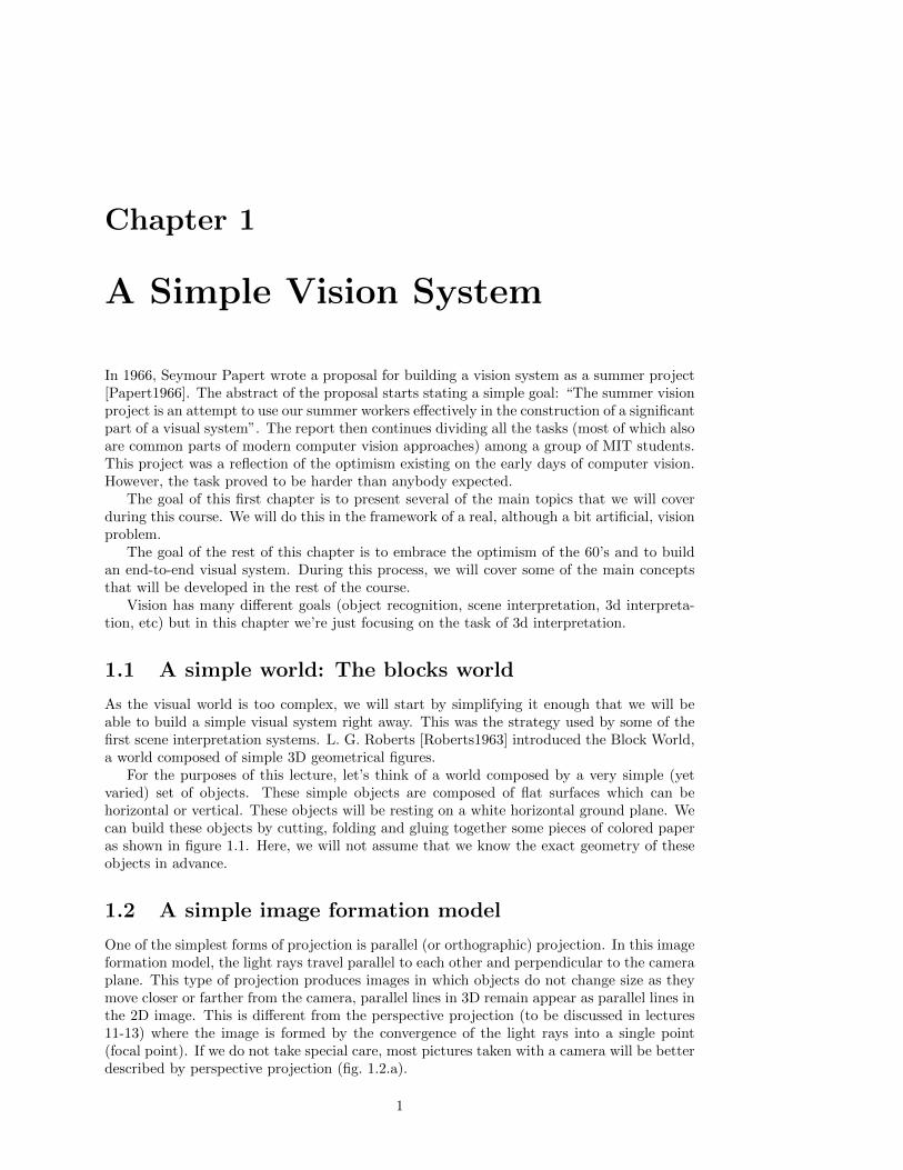
For the purposes of this lecture, let’s think of a world composed by a very simple (yetvaried) set of objects. These simple objects are composed of flat surfaces which can behorizontal or vertical. These objects will be resting on a white horizontal ground plane. Wecan build these objects by cutting, folding and gluing together some pieces of colored paperas shown in figure 1.1. Here, we will not assume that we know the exact geometry of theseobjects in advance.

1.2 A simple image formation model

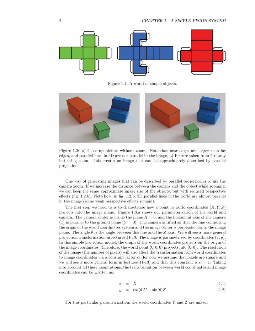
One of the simplest forms of projection is parallel (or orthographic) projection. In this imageformation model, the light rays travel parallel to each other and perpendicular to the cameraplane. This type of projection produces images in which objects do not change size as theymove closer or farther from the camera, parallel lines in 3D remain appear as parallel lines inthe 2D image. This is different from the perspective projection (to be discussed in lectures11-13) where the image is formed by the convergence of the light rays into a single point(focal point). If we do not take special care, most pictures taken with a camera will be betterdescribed by perspective projection (fig. 1.2.a).

1

2 CHAPTER 1. A SIMPLE VISION SYSTEM

Figure 1.1: A world of simple objects.

Figure 1.2: a) Close up picture without zoom. Note that near edges are larger than faredges, and parallel lines in 3D are not parallel in the image, b) Picture taken from far awaybut using zoom. This creates an image that can be approximately described by parallelprojection.

One way of generating images that can be described by parallel projection is to use thecamera zoom. If we increase the distance between the camera and the object while zooming,we can keep the same approximate image size of the objects, but with reduced perspectiveeffects (fig. 1.2.b). Note how, in fig. 1.2.b, 3D parallel lines in the world are almost parallelin the image (some weak perspective effects remain).

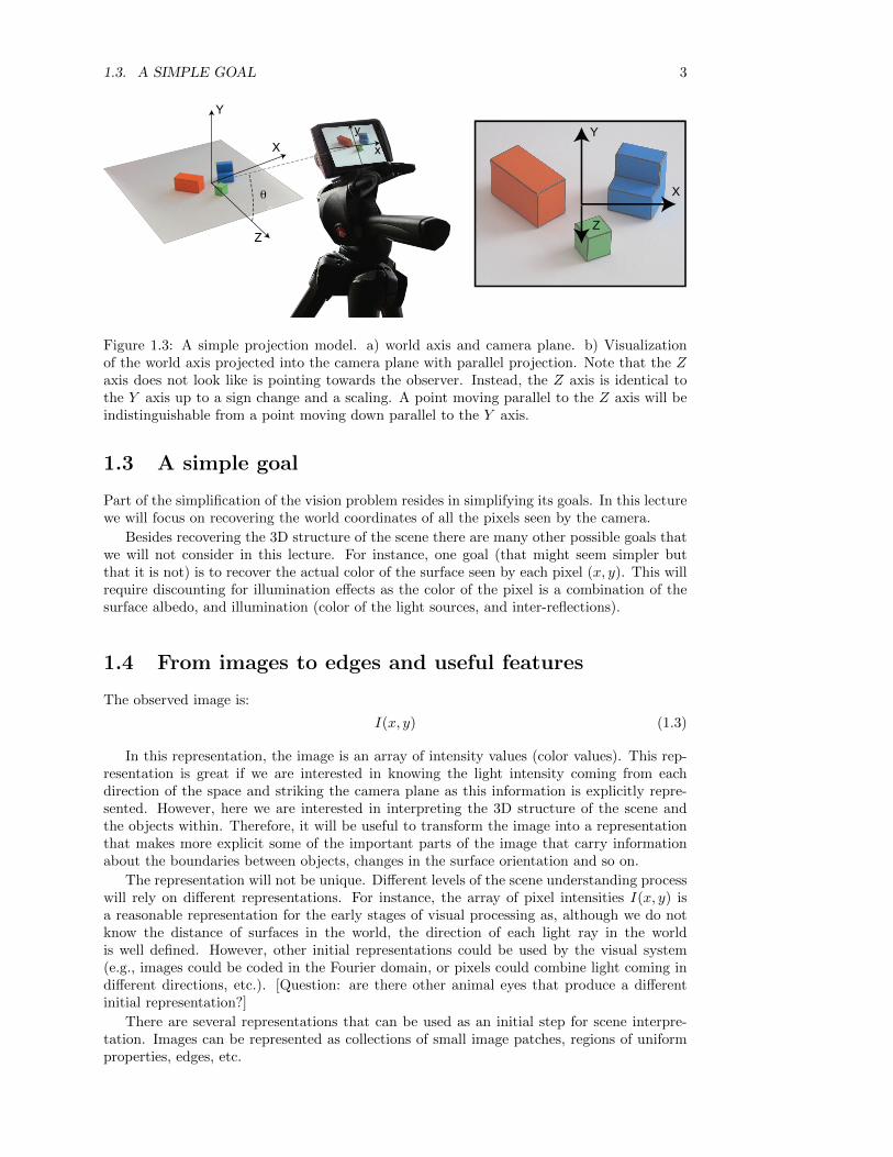
The first step we need to is to characterize how a point in world coordinates (X,Y, Z)projects into the image plane. Figure 1.3.a shows our parameterization of the world andcamera. The camera center is inside the plane X = 0, and the horizontal axis of the camera(x) is parallel to the ground plane (Y = 0). The camera is tilted so that the line connectingthe origin of the world coordinates system and the image center is perpendicular to the imageplane. The angle θ is the angle between this line and the Z axis. We will see a more generalprojection transformation in lectures 11-13. The image is parametrized by coordinates (x, y).In this simple projection model, the origin of the world coordinates projects on the origin ofthe image coordinates. Therefore, the world point (0, 0, 0) projects into (0, 0). The resolutionof the image (the number of pixels) will also affect the transformation from world coordinatesto image coordinates via a constant factor α (for now we assume that pixels are square andwe will see a more general form in lectures 11-13) and that this constant is α = 1. Takinginto account all these assumptions, the transformation between world coordinates and imagecoordinates can be written as:

x = X (1.1)

y = cos(θ)Y − sin(θ)Z (1.2)

For this particular parametrization, the world coordinates Y and Z are mixed.

1.3. A SIMPLE GOAL 3

Y

Z

X

X

Z

Y

θ

x

y

Figure 1.3: A simple projection model. a) world axis and camera plane. b) Visualizationof the world axis projected into the camera plane with parallel projection. Note that the Zaxis does not look like is pointing towards the observer. Instead, the Z axis is identical tothe Y axis up to a sign change and a scaling. A point moving parallel to the Z axis will beindistinguishable from a point moving down parallel to the Y axis.

1.3 A simple goal

Part of the simplification of the vision problem resides in simplifying its goals. In this lecturewe will focus on recovering the world coordinates of all the pixels seen by the camera.

Besides recovering the 3D structure of the scene there are many other possible goals thatwe will not consider in this lecture. For instance, one goal (that might seem simpler butthat it is not) is to recover the actual color of the surface seen by each pixel (x, y). This willrequire discounting for illumination effects as the color of the pixel is a combination of thesurface albedo, and illumination (color of the light sources, and inter-reflections).

1.4 From images to edges and useful features

The observed image is:

I(x, y) (1.3)

In this representation, the image is an array of intensity values (color values). This rep-resentation is great if we are interested in knowing the light intensity coming from eachdirection of the space and striking the camera plane as this information is explicitly repre-sented. However, here we are interested in interpreting the 3D structure of the scene andthe objects within. Therefore, it will be useful to transform the image into a representationthat makes more explicit some of the important parts of the image that carry informationabout the boundaries between objects, changes in the surface orientation and so on.

The representation will not be unique. Different levels of the scene understanding processwill rely on different representations. For instance, the array of pixel intensities I(x, y) isa reasonable representation for the early stages of visual processing as, although we do notknow the distance of surfaces in the world, the direction of each light ray in the worldis well defined. However, other initial representations could be used by the visual system(e.g., images could be coded in the Fourier domain, or pixels could combine light coming indifferent directions, etc.). [Question: are there other animal eyes that produce a differentinitial representation?]

There are several representations that can be used as an initial step for scene interpre-tation. Images can be represented as collections of small image patches, regions of uniformproperties, edges, etc.

4 CHAPTER 1. A SIMPLE VISION SYSTEM

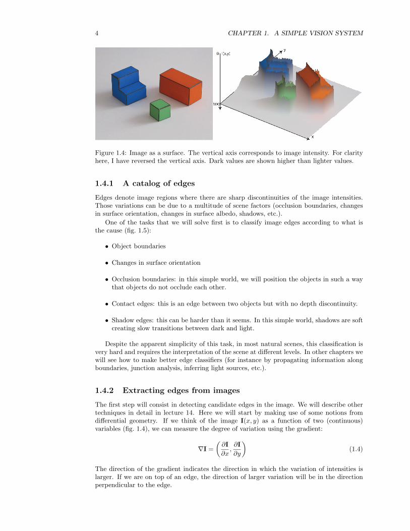
Figure 1.4: Image as a surface. The vertical axis corresponds to image intensity. For clarityhere, I have reversed the vertical axis. Dark values are shown higher than lighter values.

1.4.1 A catalog of edges

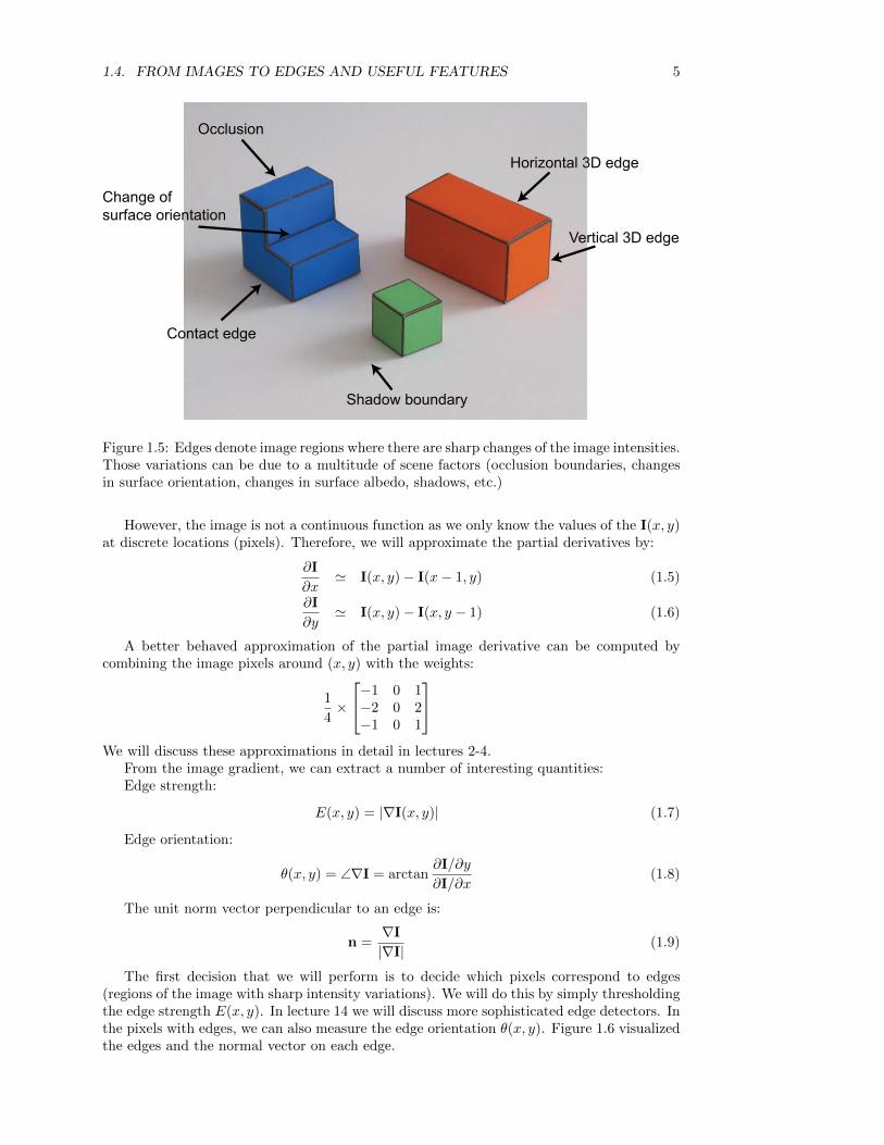
Edges denote image regions where there are sharp discontinuities of the image intensities.Those variations can be due to a multitude of scene factors (occlusion boundaries, changesin surface orientation, changes in surface albedo, shadows, etc.).

One of the tasks that we will solve first is to classify image edges according to what isthe cause (fig. 1.5):

• Object boundaries

• Changes in surface orientation

• Occlusion boundaries: in this simple world, we will position the objects in such a waythat objects do not occlude each other.

• Contact edges: this is an edge between two objects but with no depth discontinuity.

• Shadow edges: this can be harder than it seems. In this simple world, shadows are softcreating slow transitions between dark and light.

Despite the apparent simplicity of this task, in most natural scenes, this classification isvery hard and requires the interpretation of the scene at different levels. In other chapters wewill see how to make better edge classifiers (for instance by propagating information alongboundaries, junction analysis, inferring light sources, etc.).

1.4.2 Extracting edges from images

The first step will consist in detecting candidate edges in the image. We will describe othertechniques in detail in lecture 14. Here we will start by making use of some notions fromdifferential geometry. If we think of the image I(x, y) as a function of two (continuous)variables (fig. 1.4), we can measure the degree of variation using the gradient:

∇I =

(∂I

∂x,∂I

∂y

)(1.4)

The direction of the gradient indicates the direction in which the variation of intensities islarger. If we are on top of an edge, the direction of larger variation will be in the directionperpendicular to the edge.

1.4. FROM IMAGES TO EDGES AND USEFUL FEATURES 5

Occlusion

Change of

surface orientation

Contact edge

Shadow boundary

Horizontal 3D edge

Vertical 3D edge

Figure 1.5: Edges denote image regions where there are sharp changes of the image intensities.Those variations can be due to a multitude of scene factors (occlusion boundaries, changesin surface orientation, changes in surface albedo, shadows, etc.)

However, the image is not a continuous function as we only know the values of the I(x, y)at discrete locations (pixels). Therefore, we will approximate the partial derivatives by:

∂I

∂x' I(x, y)− I(x− 1, y) (1.5)

∂I

∂y' I(x, y)− I(x, y − 1) (1.6)

A better behaved approximation of the partial image derivative can be computed bycombining the image pixels around (x, y) with the weights:

1

4×

−1 0 1−2 0 2−1 0 1

We will discuss these approximations in detail in lectures 2-4.

From the image gradient, we can extract a number of interesting quantities:Edge strength:

E(x, y) = |∇I(x, y)| (1.7)

Edge orientation:

θ(x, y) = ∠∇I = arctan∂I/∂y

∂I/∂x(1.8)

The unit norm vector perpendicular to an edge is:

n =∇I|∇I|

(1.9)

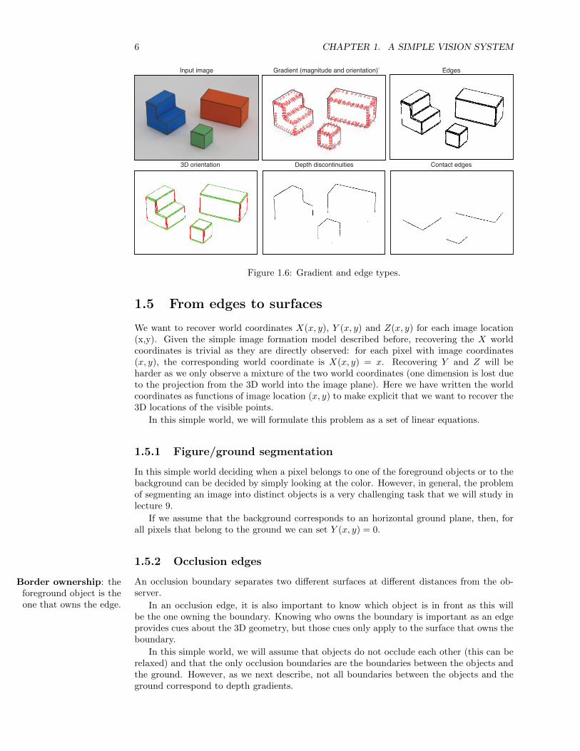
The first decision that we will perform is to decide which pixels correspond to edges(regions of the image with sharp intensity variations). We will do this by simply thresholdingthe edge strength E(x, y). In lecture 14 we will discuss more sophisticated edge detectors. Inthe pixels with edges, we can also measure the edge orientation θ(x, y). Figure 1.6 visualizedthe edges and the normal vector on each edge.

6 CHAPTER 1. A SIMPLE VISION SYSTEM

Input image EdgesGradient (magnitude and orientation)`

3D orientation Depth discontinuities Contact edges

Figure 1.6: Gradient and edge types.

1.5 From edges to surfaces

We want to recover world coordinates X(x, y), Y (x, y) and Z(x, y) for each image location(x,y). Given the simple image formation model described before, recovering the X worldcoordinates is trivial as they are directly observed: for each pixel with image coordinates(x, y), the corresponding world coordinate is X(x, y) = x. Recovering Y and Z will beharder as we only observe a mixture of the two world coordinates (one dimension is lost dueto the projection from the 3D world into the image plane). Here we have written the worldcoordinates as functions of image location (x, y) to make explicit that we want to recover the3D locations of the visible points.

In this simple world, we will formulate this problem as a set of linear equations.

1.5.1 Figure/ground segmentation

In this simple world deciding when a pixel belongs to one of the foreground objects or to thebackground can be decided by simply looking at the color. However, in general, the problemof segmenting an image into distinct objects is a very challenging task that we will study inlecture 9.

If we assume that the background corresponds to an horizontal ground plane, then, forall pixels that belong to the ground we can set Y (x, y) = 0.

1.5.2 Occlusion edges

An occlusion boundary separates two different surfaces at different distances from the ob-server.

Border ownership: theforeground object is theone that owns the edge. In an occlusion edge, it is also important to know which object is in front as this will

be the one owning the boundary. Knowing who owns the boundary is important as an edgeprovides cues about the 3D geometry, but those cues only apply to the surface that owns theboundary.

In this simple world, we will assume that objects do not occlude each other (this can berelaxed) and that the only occlusion boundaries are the boundaries between the objects andthe ground. However, as we next describe, not all boundaries between the objects and theground correspond to depth gradients.

1.5. FROM EDGES TO SURFACES 7

1.5.3 Contact edges

Contact edges are boundaries between two distinct objects but where there exists no depthdiscontinuity. Despite that there is not depth discontinuity, there is an occlusion here (asone surface is hidden behind another), and the edge shape is only owned by one of the twosurfaces.

In this simple world, if we assume that all the objects rest on the ground plane, then wecan set Y (x, y) = 0 on the contact edges.

Contact edges can be detected as transitions between object (above) and ground (below).In the simple world only horizontal edges can be contact edges. We will discuss next how toclassify edges according to their 3D orientation.

1.5.4 Generic view and non-accidental scene properties

Despite that in the projection of world coordinates to image coordinates we have lost a greatdeal of information, there are a number of properties that will remain invariant and can helpus in interpreting the image. Here is a list of some of those invariant properties (we willdiscuss some of them in depth in lecture 11 when talking about camera geometry):

• Collinearity: a straight 3D line will project into a straight line in the image.

• Cotermination: if two or more 3D lines terminate at the same point, the correspondingprojections will also terminate at a common point.

• Intersection: if two 3D lines intersect at a point, the projection will result in twointersecting lines

• Parallelism: (under weak perspective)

• Symmetry (under weak perspective)

• Smoothness: a smooth 3D curve will project into a smooth 2D curve.

Note that those invariances refer to the process of going from world coordinates to imagecoordinates. The opposite might not be true. For instance, a straight line in the image couldcorrespond to a curved line in the 3D world but that happens to be precisely aligned withrespect to the viewers point of view to appear as a straight line. Also, two lines that intersectin the image plane could be disjoint in the 3D space.

However, some of these properties (not all), while not always true, can nonetheless beused to reliably infer something about the 3D world using a single 2D image as input. Forinstance, if two lines coterminate in the image, then, one can conclude that it is very likelythat they also touch each other in 3D. If the 3D lines do not touch each other, then it willrequire a very specific alignment between the observer and the lines for them to appear tocoterminate in the image. Therefore, one can safely conclude that the lines might also touchin 3D.

These properties are called non-accidental properties as they will only be observed in theimage if they also exist in the world or by accidental alignments between the observer andscene structures. Under a generic view, nonaccidental properties will be shared by the imageand the 3D world.

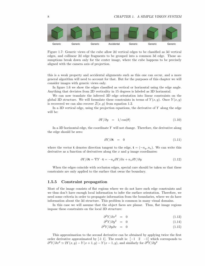
Let’s see how this idea applies to our simple world. In this simple world all 3D edgesare either vertical or horizontal. Under parallel projection, we will assume that 2D verticaledges are also 3D vertical edges. Under parallel projection and with the camera havingits horizontal axis parallel to the ground, we know that vertical 3D lines will project intovertical 2D lines in the image. On the other hand, horizontal lines will, in general, projectinto oblique lines. Therefore, we can assume than any vertical line in the image is also avertical line in the world. As shown in figure 1.7, in the case of the cube, there is a particularviewpoint that will make an horizontal line project into a vertical line, but this will requirean accidental alignment between the cube and the line of sight of the observer. Nevertheless,

8 CHAPTER 1. A SIMPLE VISION SYSTEM

Generic Generic Generic Generic Generic GenericAccidental

Figure 1.7: Generic views of the cube allow 2d vertical edges to be classified as 3d verticaledges, and collinear 2d edge fragments to be grouped into a common 3d edge. Those as-sumptions break down only for the center image, where the cube happens to be preciselyaligned with the camera axis of projection.

this is a weak property and accidental alignments such as this one can occur, and a moregeneral algorithm will need to account for that. But for the purposes of this chapter we willconsider images with generic views only.

In figure 1.6 we show the edges classified as vertical or horizontal using the edge angle.Anything that deviates from 2D verticality in 15 degrees is labeled as 3D horizontal.

We can now translate the inferred 3D edge orientation into linear constraints on theglobal 3D structure. We will formulate these constraints in terms of Y (x, y). Once Y (x, y)is recovered we can also recover Z(x, y) from equation 1.2.

In a 3D vertical edge, using the projection equations, the derivative of Y along the edgewill be:

∂Y/∂y = 1/ cos(θ) (1.10)

In a 3D horizontal edge, the coordinate Y will not change. Therefore, the derivative alongthe edge should be zero:

∂Y/∂t = 0 (1.11)

where the vector t denotes direction tangent to the edge, t = (−ny, nx). We can write thisderivative as a function of derivatives along the x and y image coordinates:

∂Y/∂t = ∇Y · t = −ny∂Y/∂x+ nx∂Y/∂y (1.12)

When the edges coincide with occlusion edges, special care should be taken so that theseconstraints are only applied to the surface that owns the boundary.

1.5.5 Constraint propagation

Most of the image consists of flat regions where we do not have such edge constraints andwe thus don’t have enough local information to infer the surface orientation. Therefore, weneed some criteria in order to propagate information from the boundaries, where we do haveinformation about the 3d structure. This problem is common in many visual domains.

In this case we will assume that the object faces are planar. Thus, flat image regionsimpose these constraints on the local 3D structure:

∂2Y/∂x2 = 0 (1.13)

∂2Y/∂y2 = 0 (1.14)

∂2Y/∂y∂x = 0 (1.15)

This approximation to the second derivative can be obtained by applying twice the firstorder derivative approximated by [-1 1]. The result is:

[−1 2 −1

]which corresponds to

∂2Y/∂x2 ' 2Y (x, y)− Y (x+ 1, y)− Y (x− 1, y), and similarly for ∂2Y/∂y2

1.5. FROM EDGES TO SURFACES 9

1.5.6 A simple inference scheme

All the different constraints described before can be written as an overdetermined system oflinear equations. Each equation will have the form:

aiY = bi (1.16)

Note that there might be many more equations than there are image pixels.

We can translate all the constraints described in the previous sections into this form. Forinstance, if the index i corresponds to one of the pixels inside one of the planar faces of a fore-ground object, then the planarity constraint can be written as ai = [0, . . . , 0,−1, 2,−1, 0, . . . , 0],bi = 0.

We can solve the system of equations by minimizing the following cost function:

J =∑i

(aiY − bi)2 (1.17)

If some constraints are more important than others, it is possible to also add a weightwi.

J =∑i

wi(aiY − bi)2 (1.18)

It is a big system of linear constraints and it can also be written in matrix form:

AY = b (1.19)

where row i of the matrix A contains the constraint coefficients ai. This problem can besolved efficiently as the matrix A is very sparse (most of the elements are zero).

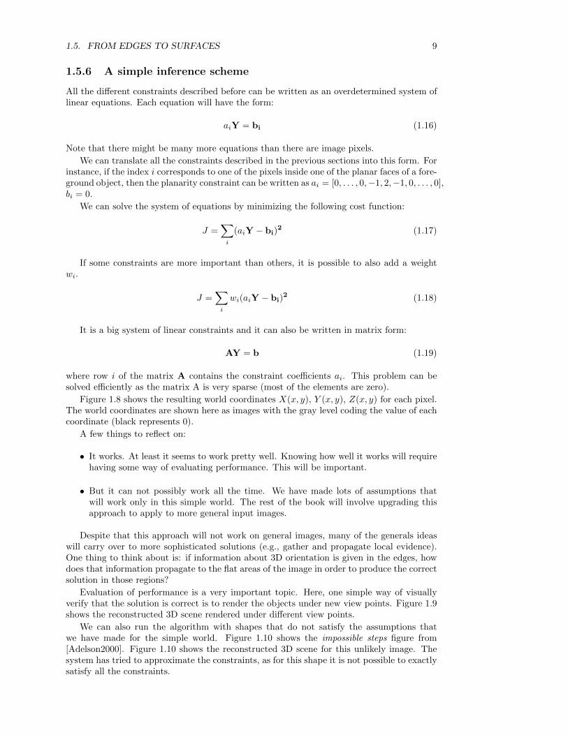
Figure 1.8 shows the resulting world coordinates X(x, y), Y (x, y), Z(x, y) for each pixel.The world coordinates are shown here as images with the gray level coding the value of eachcoordinate (black represents 0).

A few things to reflect on:

• It works. At least it seems to work pretty well. Knowing how well it works will requirehaving some way of evaluating performance. This will be important.

• But it can not possibly work all the time. We have made lots of assumptions thatwill work only in this simple world. The rest of the book will involve upgrading thisapproach to apply to more general input images.

Despite that this approach will not work on general images, many of the generals ideaswill carry over to more sophisticated solutions (e.g., gather and propagate local evidence).One thing to think about is: if information about 3D orientation is given in the edges, howdoes that information propagate to the flat areas of the image in order to produce the correctsolution in those regions?

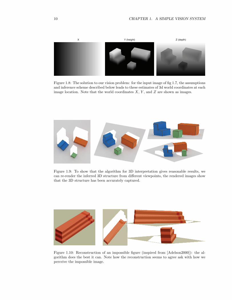
Evaluation of performance is a very important topic. Here, one simple way of visuallyverify that the solution is correct is to render the objects under new view points. Figure 1.9shows the reconstructed 3D scene rendered under different view points.

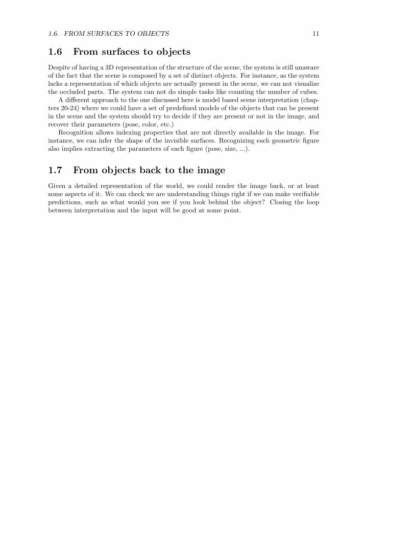
We can also run the algorithm with shapes that do not satisfy the assumptions thatwe have made for the simple world. Figure 1.10 shows the impossible steps figure from[Adelson2000]. Figure 1.10 shows the reconstructed 3D scene for this unlikely image. Thesystem has tried to approximate the constraints, as for this shape it is not possible to exactlysatisfy all the constraints.

10 CHAPTER 1. A SIMPLE VISION SYSTEM

Z (depth)Y (height)X

Figure 1.8: The solution to our vision problem: for the input image of fig 1.7, the assumptionsand inference scheme described below leads to these estimates of 3d world coordinates at eachimage location. Note that the world coordinates X, Y , and Z are shown as images.

Figure 1.9: To show that the algorithm for 3D interpretation gives reasonable results, wecan re-render the inferred 3D structure from different viewpoints, the rendered images showthat the 3D structure has been accurately captured.

Figure 1.10: Reconstruction of an impossible figure (inspired from [Adelson2000]): the al-gorithm does the best it can. Note how the reconstruction seems to agree ask with how weperceive the impossible image.

1.6. FROM SURFACES TO OBJECTS 11

1.6 From surfaces to objects

Despite of having a 3D representation of the structure of the scene, the system is still unawareof the fact that the scene is composed by a set of distinct objects. For instance, as the systemlacks a representation of which objects are actually present in the scene, we can not visualizethe occluded parts. The system can not do simple tasks like counting the number of cubes.

A different approach to the one discussed here is model based scene interpretation (chap-ters 20-24) where we could have a set of predefined models of the objects that can be presentin the scene and the system should try to decide if they are present or not in the image, andrecover their parameters (pose, color, etc.)

Recognition allows indexing properties that are not directly available in the image. Forinstance, we can infer the shape of the invisible surfaces. Recognizing each geometric figurealso implies extracting the parameters of each figure (pose, size, ...).

1.7 From objects back to the image

Given a detailed representation of the world, we could render the image back, or at leastsome aspects of it. We can check we are understanding things right if we can make verifiablepredictions, such as what would you see if you look behind the object? Closing the loopbetween interpretation and the input will be good at some point.

12 CHAPTER 1. A SIMPLE VISION SYSTEM

Bibliography

[Adelson2000] Adelson, Edward H. 2000. Lightness perception and lightness illusion. In Thenew cognitive neurosciences, ed. M. Gazzaniga, 339–351.

[Papert1966] Papert, Seymour. 1966. The summer vision project, MIT AI Memo 100, Mas-sachusetts Institute of Technology, Project Mac.

[Roberts1963] Roberts, Lawrence G. 1963. Machine perception of three-dimensional solids.Outstanding dissertations in the computer sciences. Garland Publishing, New York.

13