A Simplified Economic Filter for Open-Pit Mining and Heap-Leach Recovery of Copper in the United States By Keith R. Long1 and Donald A. Singer2

Open-File Report 01-218

2001

This report is preliminary and has not been reviewed for conformity with U.S. Geological Survey editorial standards or with the North American Stratigraphic Code. Any use of trade, firm, or product names is for descriptive purposes only and does not imply endorsement by the U.S. Government.

U.S. DEPARTMENT OF THE INTERIOR U.S. Geological Survey

1 520 North Park Avenue, Suite 355, Tucson, AZ 85719 2 345 Middlefield Road, Menlo Park, CA 94025

ii

Contents

Summary ........................................................................................... 1

Introduction ...................................................................................... 1

General Considerations................................................................... 2

Empirical Analysis of Cost Data ..................................................... 3

Evaluation of Camm (1991) Cost Model ......................................... 9

Application Example ...................................................................... 15

Conclusions.................................................................................... 17

References Cited ............................................................................ 17

Figures Figure 1. Relationship between mining rate (ore and waste) and capital cost for open-pit heap-leach SX/EW copper mines. Regression line (r = 0.83) and 95 percent confidence interval shown. ..................................................................................................................7 Figure 2. Relationship between mining rate (ore and waste) and operating cost for open-pit heap-leach SX/EW copper mines. Regression line (r = -0.75) and 95 percent confidence interval shown.................................................................................................8

Tables Table 1. Cost and operating data for selected mines .....................................................5 Table 2. Cost indexes for updating cost models . .........................................................12 Table 3. Comparison of estimated costs with actual values . .......................................14

iii

Table 4. Comparison of estimates using empirical and Camm (1991) models . ...........16 Table 5. Comparison of net present value calculations using each model . .................16

Conversion Factors

Multiply By To Obtain

Length meter (m) 3.280

8 foot

Mass kilogram (kg) 2.204

6 pound

metric ton (mt)

1.1023

short ton

1

Summary Determining the economic viability of mineral deposits of various sizes and grades is

a critical task in all phases of mineral supply, from land-use management to mine development. This study evaluates two simple tools for estimating the economic viability of porphyry copper deposits mined by open-pit, heap-leach methods when only limited information on these deposits is available. These two methods are useful for evaluating deposits that either (1) are undiscovered deposits predicted by a mineral resource assessment, or (2) have been discovered but for which little data has been collected or released. The first tool uses ordinary least-squared regression analysis of cost and operating data from selected deposits to estimate a predictive relationship between mining rate, itself estimated from deposit size, and capital and operating costs. The second method uses cost models developed by the U.S. Bureau of Mines (Camm, 1991) updated using appropriate cost indices. We find that the cost model method works best for estimating capital costs and the empirical model works best for estimating operating costs for mines to be developed in the United States.

Introduction Mining firms must discriminate between mineral deposits that are economic or

uneconomic to develop for production. The primary tool for this task is a feasibility study which compares alternative mine designs to identify the least-costly method of mining the deposit and estimates financial returns given likely scenarios for future mineral prices and input costs. Feasibility studies require considerable geologic and engineering data to accurately estimate mining costs. These data are not available until a deposit has been thoroughly investigated by drilling, sampling, and metallurgical testing. There is a need, however, for a simple tool to discriminate between economic and uneconomic deposits that have not been fully explored or have not yet been discovered. Known as economic filters or cost-models, these tools may be used in exploration to determine which of alternative areas or deposits have the greatest economic potential. In resource assessment, these filters can help determine which of the deposits forecasted will be economic or uneconomic when discovered. Although filters require much less data, they are significantly less precise in their predictions than feasibility studies.

The U.S. Bureau of Mines (USBM) developed simplified cost-models (Camm, 1991; Smith, 1992). In two previous studies, Singer and others (1998) and Singer and others (2000), developed simplified economic filters for open-pit gold mining and underground mining of massive sulfide deposits, respectively. These studies tested the models of Camm (1991) and made modifications where appropriate. O’Hara and Suboleski (1992) proposed a more complex method of cost estimation appropriate to detailed pre-feasibility studies. Stanley (1994) developed a cost-model for open-pit mining, flotation concentration, and heap-leaching of copper using commercially available mining cost estimating software and mineral processing models of Camm (1991).

This paper assesses two methods of cost-modeling for open-pit mining and heap-leaching of copper ores with copper recovery by solvent-extraction and electrowinning (SX/EW). We exclude consideration of conventional flotation concentration of copper because almost all recent and proposed open-pit copper mining projects in the United

2

States use heap- and dump-leaching methods exclusively. The two approaches considered are (1) an empirical model which relates mining costs to mining rates using data from recently developed or proposed copper mines; and (2) the original Camm (1991) models, updated using appropriate cost inflators. The cost models of O’Hara and Suboleski (1991) and Stanley (1994) were not evaluated because they do not model costs of in-pit crushing, construction of heaps, heap-leaching, and solvent extraction of copper. Commercially available mine-costing software could not be evaluated for the same reasons.

General Considerations Large copper deposits are mostly mined by open-pit methods, although a few

deposits are mined underground by block-caving. Ores mined are normally processed by bulk or selective flotation to yield concentrates which are further processed at a smelter. Selective flotation is used to recover molybdenum as a byproduct in a separate concentrate. Gold and silver are common byproducts in copper concentrates and are recovered with copper at the smelter and refinery. Another method of copper recovery, leaching of copper from run-of-mine or crushed ore placed on dumps, followed by extraction of highly-pure copper from the leach solutions by solution extraction and electrowinning (SX-EW), is increasingly used due to its relatively low costs. Not all ores are amenable to leaching, hence many mines employ both methods. A few mines extract additional copper by leaching ore in-place, generally in abandoned underground mine workings. In-place leaching of unmined deposits is a technology currently under development. Almost all copper mines recently proposed for development in the United States plan to use heap-leach SX-EW methods exclusively, hence we only consider this technology in developing a copper filter for mining porphyry copper deposits.

Any cost model can be tested by applying it to mines whose costs are known or to development projects whose costs have been modeled in great detail by a formal feasibility study. In the case of domestic copper producers, such a comparison is hampered by a policy of most producers not to release cost data. An exhaustive literature search yielded scant anecdotal data on operating costs and a limited amount of capital cost data for operating mines and proposed projects in the United States.

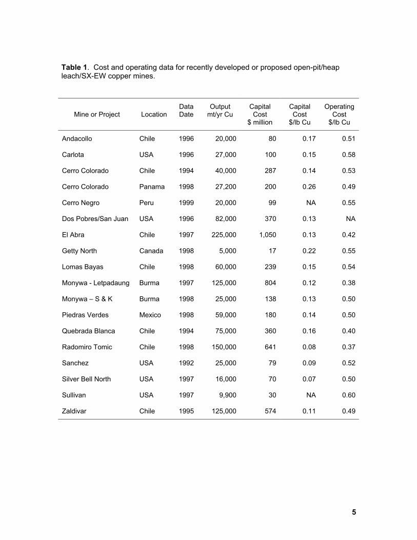
Cost data is much easier to obtain for mines in Canada, Chile, and other major copper producing countries. Of these, only mines in Chile use heap-leaching to any great extent as the sole means of copper recovery. Available data that are of use to this study are listed in table 1. Data were collected for this study from a wide variety of industry sources, principally company annual reports and annual filings with regulatory agencies, press releases, and reports in the mining press. Deposits were classified as economic at a particular price of copper if they were developed into operating mines that have operated at that price or if a feasibility study reports that a proposed mine is economic at that price.

There are valid questions concerning the comparability of capital and operating costs between U.S. and foreign mines. The comparative lack of infrastructure in some foreign countries might add significantly to capital costs. Costs of machinery, energy, and other supplies might be higher, particularly if they must be imported.

3

Copper mining is a capital-intensive industry engaged in continuous innovation to reduce operating costs sufficiently to offset declining ore grades and competition from lower-cost sources. Lower operating costs are obtained through increasing economies of scale and labor productivity, which require substitution of capital for labor. In real terms, these efforts should result in increasing capital costs and decreasing operating costs over time for the development and operation of a mine of any given capacity. This raises the question whether cost models developed ten years ago will still be valid.

There is good reason to believe that the Camm (1991) cost models have not been invalidated by a changing cost structure in the copper industry. Tilton and Landsberg (1997) show that increases of labor productivity in the domestic copper industry occur during relatively short time intervals separated by periods of stability or gradual decline. The last period of innovation was from 1980 to 1986, after which labor productivity has changed little. Operating-cost reductions continue, but are the result not of industry-wide improvements in labor productivity but of ongoing substitution of a relatively new technology for recovering copper, heap-leach and SX/EW, which is significantly less expensive than conventional flotation concentration, smelting, and refining.

Copper industry practice for reporting operating costs is incompatible with the simplified cost models of Camm (1991). The Camm (1991) cost models estimate mining and milling costs separately and exclude byproduct credits and smelting, refining, and transportation costs. Mining costs are modeled in terms of U.S. dollars per ton of ore and waste mined and milling costs in terms of U.S. dollars per ton of ore processed; hence the two costs models cannot be added together to yield mining and milling operating costs on a common basis such as per tons of ore mined and milled without conversion. To determine if a deposit is economic using the models of Camm (1991), one must first calculate total life-of-mine capital and operating costs and compare them with total life-of-mine revenues, including byproduct credits, net of smelting, refining, and transportation costs. This operating profit is then compared with total capital costs to determine if these costs are covered with sufficient return on capital to justify developing the mine. To determine if a deposit is economic using industry cost data, one compares the operating cost with an assumed long-term average price of copper. If there is an operating profit, one then determines if it is sufficient to recover capital expenditures with interest. A better procedure for determining profitability is to calculate the present value of estimated net income over the life of the project. This requires assumptions as to the timing of future expenditures and revenue streams, future copper prices and the appropriate interest rate. Smith, 1992, follows such a procedure, using Camm’s, 1991, equations.

Empirical Analysis of Cost Data A simple approach for a cost-model would be to correlate operating and capital costs

with mine capacity. The resulting equations would be easier to use than those of Camm (1991) because mining and processing costs are combined and costs are presented in a way that conforms to industry practice. If these equations are valid, to determine if a deposit is economic, one can calculate the net present value of estimated future net revenues from mining the deposit. A deposit is economic if there is sufficient surplus to cover interest on capital. Note that for the copper recovery method under consideration

4

here, heap-leach SX-EW, there will be no byproduct credits and the output is already a refined product.

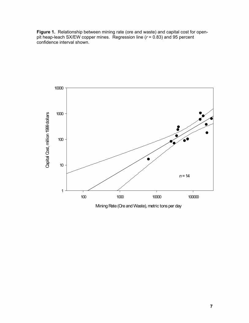
Figure 1 shows the results of a linear regression of capital costs in million dollars against mine capacity in terms of ore and waste mined per day using data from table 1 updated to 1999 dollars using cost indices from table 2. The fitted regression equation is:

ln 4.123 0.846ln OWK X= − + (1)

where K is capital cost in million dollars and OWX operating rate (ore plus waste) in metric tons per day. The correlation coefficient (r) is 0.83.

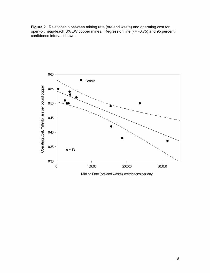
Figure 2 shows the results of a linear regression of operating costs per pound of copper recovered against mine capacity in terms of ore and waste mined per day. Data are from table 1 updated to 1999 dollars using cost indices from table 2. There are no special considerations that would warrant removal of one outlier (Carlota project), hence it was retained, although it should be noted that it is highly unlikely that reported operating costs for Carlota were calculated in the same way as the other deposits. It is possible that the relatively high operating cost reported for Carlota might include an allowance for capital depreciation. The fitted regression equation is:

70.565 5.563 OWC X−= − (2)

where C is operating cost in dollars per pound copper and OWX is operating rate (ore plus waste) in metric tons per day. The correlation coefficient (r) is –0.75.

5

Table 1. Cost and operating data for recently developed or proposed open-pit/heap leach/SX-EW copper mines.

Mine or Project

Location

Data Date

Output mt/yr Cu

Capital Cost

$ million

Capital Cost

$/lb Cu

Operating Cost

$/lb Cu

Andacollo Chile 1996 20,000 80 0.17 0.51

Carlota USA 1996 27,000 100 0.15 0.58

Cerro Colorado Chile 1994 40,000 287 0.14 0.53

Cerro Colorado Panama 1998 27,200 200 0.26 0.49

Cerro Negro Peru 1999 20,000 99 NA 0.55

Dos Pobres/San Juan USA 1996 82,000 370 0.13 NA

El Abra Chile 1997 225,000 1,050 0.13 0.42

Getty North Canada 1998 5,000 17 0.22 0.55

Lomas Bayas Chile 1998 60,000 239 0.15 0.54

Monywa - Letpadaung Burma 1997 125,000 804 0.12 0.38

Monywa – S & K Burma 1998 25,000 138 0.13 0.50

Piedras Verdes Mexico 1998 59,000 180 0.14 0.50

Quebrada Blanca Chile 1994 75,000 360 0.16 0.40

Radomiro Tomic Chile 1998 150,000 641 0.08 0.37

Sanchez USA 1992 25,000 79 0.09 0.52

Silver Bell North USA 1997 16,000 70 0.07 0.50

Sullivan USA 1997 9,900 30 NA 0.60

Zaldivar Chile 1995 125,000 574 0.11 0.49

6

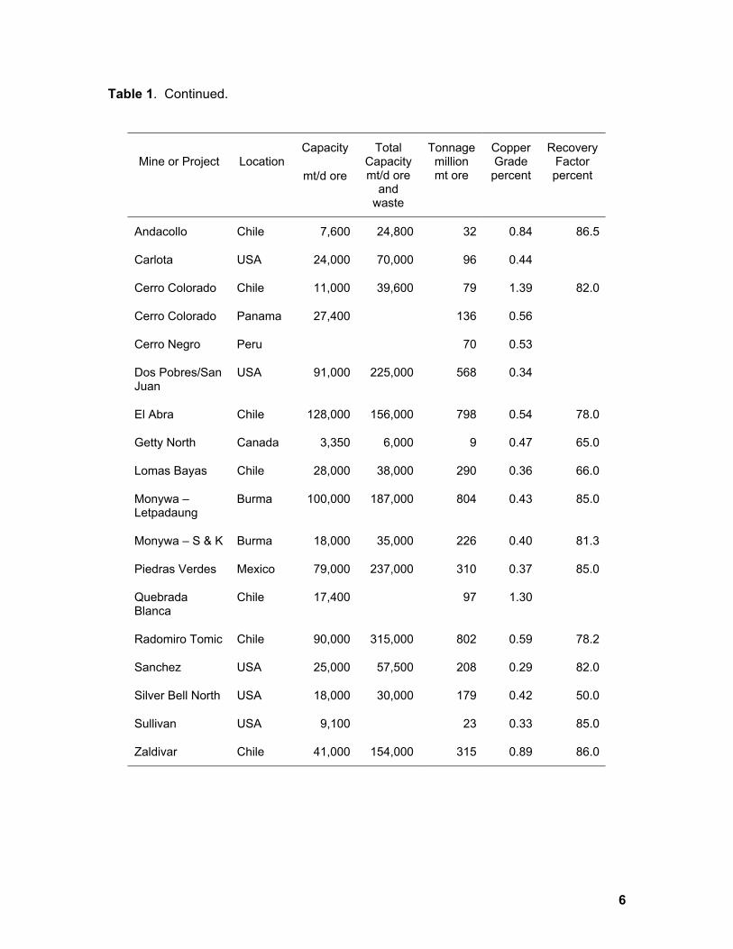
Table 1. Continued.

Mine or Project

Location

Capacity

mt/d ore

Total Capacitymt/d ore

and waste

Tonnagemillion mt ore

Copper Grade percent

Recovery Factor percent

Andacollo Chile 7,600 24,800 32 0.84 86.5

Carlota USA 24,000 70,000 96 0.44

Cerro Colorado Chile 11,000 39,600 79 1.39 82.0

Cerro Colorado Panama 27,400 136 0.56

Cerro Negro Peru 70 0.53

Dos Pobres/San Juan

USA 91,000 225,000 568 0.34

El Abra Chile 128,000 156,000 798 0.54 78.0

Getty North Canada 3,350 6,000 9 0.47 65.0

Lomas Bayas Chile 28,000 38,000 290 0.36 66.0

Monywa – Letpadaung

Burma 100,000 187,000 804 0.43 85.0

Monywa – S & K Burma 18,000 35,000 226 0.40 81.3

Piedras Verdes Mexico 79,000 237,000 310 0.37 85.0

Quebrada Blanca

Chile 17,400 97 1.30

Radomiro Tomic Chile 90,000 315,000 802 0.59 78.2

Sanchez USA 25,000 57,500 208 0.29 82.0

Silver Bell North USA 18,000 30,000 179 0.42 50.0

Sullivan USA 9,100 23 0.33 85.0

Zaldivar Chile 41,000 154,000 315 0.89 86.0

7

Figure 1. Relationship between mining rate (ore and waste) and capital cost for open-pit heap-leach SX/EW copper mines. Regression line (r = 0.83) and 95 percent confidence interval shown.

Mining Rate (Ore and Waste), metric tons per day

100 1000 10000 100000

Capi

tal C

ost,

milli

on 19

99 d

olla

rs

1

10

100

1000

10000

n = 14

8

Figure 2. Relationship between mining rate (ore and waste) and operating cost for open-pit heap-leach SX/EW copper mines. Regression line (r = -0.75) and 95 percent confidence interval shown.

Mining Rate (ore and waste), metric tons per day

0 100000 200000 300000

Oper

atin

g Co

st, 1

999 d

olla

rs p

er p

ound

cop

per

0.30

0.35

0.40

0.45

0.50

0.55

0.60

n = 13

Carlota

9

Hoskins (1986) notes that preliminary feasibility studies conducted by the mining industry yield estimates of capital and operating costs that deviate as much as 100 percent from their actual values, although a 30 percent deviation is a realistic expectation if such studies are properly done. From this perspective, the two regression equations should be adequate for classification of deposits as economic or uneconomic in exploration planning and mineral resource appraisal. If the data can be found, the data and resulting equations could be improved by (1) adjusting capital costs to exclude infrastructure and other costs that do not pertain to mine development in the United States; and (2) insuring that the operating costs are calculated in the same way, in particular excluding capital depreciation.

Evaluation of Camm (1991) Cost Model The U.S. Bureau of Mines (Camm, 1991) developed simplified cost models to

estimate operating and capital expenditures for a mineral deposit given, at a minimum, data on size, grade, depth, and appropriate mining and processing methods. These cost models can be adjusted using additional data on haulage distance and some infrastructure requirements. The models were derived by fitting equations to cost data from a small number (3 to 6) of active U.S. mines. These cost data are now over ten years old and may not reflect current cost-saving technology. For example, the Camm (1991) model for open-pit mines is valid for extraction rates up to 200,000 short tons ore and waste per day, whereas some porphyry copper mines today produce more than 300,000 short tons ore and waste per day. In this section, we test the simplified cost models of Camm (1991) to determine their reliability with a set of deposits known to be economic or non-economic.

Application of Camm’s simplified cost models begins with calculating mine capacity or operating rate and, implicitly, mine life, using Taylor’s rule:

0.750.0147OX T= (3)

where OX is operating rate in metric tons of ore per day and T is total amount of ore to be mined in metric tons. The usefulness of Taylor’s rule (Taylor, 1986), based on data for many types of mines in the 1970s is not known. Hence, we have re-estimated Taylor’s rule using data from a large number (n = 45) of open-pit copper mines (including but not exclusively those in table 1):

0.740.0236OX T= (4)

Equation 4 has a correlation coefficient (r) of 0.96 but the estimated equation coefficients are not significantly different at the 5 percent probability level from those of Taylor (1986). We therefore use Taylor’s original equation (equation 3).

10

Once operating rate is established, capital and operating costs can be estimated. Camm (1991) gives equations for estimating mining and processing costs of large open-pit mines with heap-leaching/SX-EW. For mining costs, the large open-pit model estimates capital costs as:

0.9172,670m tK X= (5)

where Km is capital cost for mining in dollars and Xt is mine capacity in short tons per day ore and waste. The equation is valid for mines operating at a rate of 20,000 to 200,000 short tons of ore and waste per day. Note that Taylor’s rule computes capacity in terms of metric tons of ore per day. Independent data on the ratio of waste to ore (strip ratio) is required to recalculate mine capacity in terms or ore and waste mined per day. Operating costs are similarly estimated as:

0.1485.14m tC X −= (6)

where Cm is operating cost for mining in dollars per short ton mined and Xt is mine capacity in short tons per day ore and waste. Camm (1991), describes a procedure for adjusting for variations in haulage distance but that procedure is not used here because no data could be found on average haulage distance over the life of the mines and projects listed in table 1.

Camm (1991) gives a cost model for heap-leach SX/EW processing operations of 6,000 to 70,000 short tons per day. The model assumes an ore grade of 0.4 percent copper and a recovery of 50 percent, which deviates significantly from the copper grades and recovery factors reported for most of the mines and projects in table 1. Capital costs are estimated as:

0.59614,600 665p f fK X X= + (7)

where Kp is capital cost for processing in dollars and Xf is processing capacity in short tons per day of ore. For operating costs:

0.1453.00p fC X −= (8)

where Cp is operating cost of processing in dollars per short ton processed and Xf is processing capacity in short tons per day ore.

11

Capital costs do not include any infrastructure costs outside of the mine site. These would include access roads, power lines, water lines, housing and urban facilities for workers, transshipment facilities, etc. Many of the mines and projects in table 1 are in remote areas where much more infrastructure must be provided than if that mine or project were built in the United States. Camm (1991) gives equations for estimating capital costs of access roads and power lines. Capital costs of access roads of 18 meters width are estimated by:

3,700r rK D= (9)

where Kr is capital cost of road access in dollars and Dr is the length of access road to be constructed in miles. Capital costs of power lines with a pole height of 12 meters are estimated by:

310,400pl plK D= (10)

where Kpl is capital cost of power line in dollars and Dpl is the length of power line to be constructed in miles. Camm (1991) does not provide any means of estimating other infrastructure costs. Nor does Camm (1991) provide any models for estimating exploration and land acquisition costs or reclamation and other mine closure costs.

All of the Camm (1991) models predict costs in terms of 1989 U.S. dollars. Camm (1991) suggests several annual cost index series to update the cost equations. Table 2 gives cost indexes for the years 1990 to 1999 according to two series: (1) the Marshall & Swift mining and milling cost index for use with all mining and processing capital and operating cost equations, and (2) ENR building cost index for use with the infrastructure capital cost equations. Camm (1991) describes the procedure for updating costs using these indexes.

12

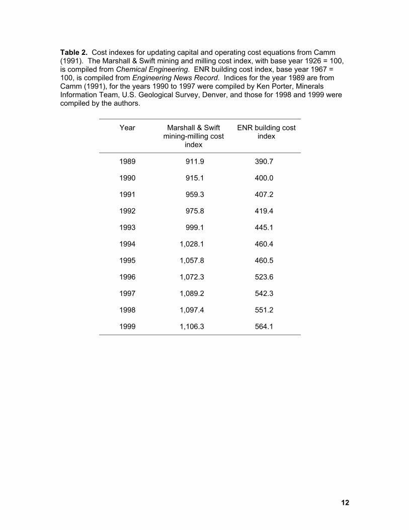
Table 2. Cost indexes for updating capital and operating cost equations from Camm (1991). The Marshall & Swift mining and milling cost index, with base year 1926 = 100, is compiled from Chemical Engineering. ENR building cost index, base year 1967 = 100, is compiled from Engineering News Record. Indices for the year 1989 are from Camm (1991), for the years 1990 to 1997 were compiled by Ken Porter, Minerals Information Team, U.S. Geological Survey, Denver, and those for 1998 and 1999 were compiled by the authors.

Year Marshall & Swift mining-milling cost

index

ENR building cost index

1989 911.9 390.7

1990 915.1 400.0

1991 959.3 407.2

1992 975.8 419.4

1993 999.1 445.1

1994 1,028.1 460.4

1995 1,057.8 460.5

1996 1,072.3 523.6

1997 1,089.2 542.3

1998 1,097.4 551.2

1999 1,106.3 564.1

13

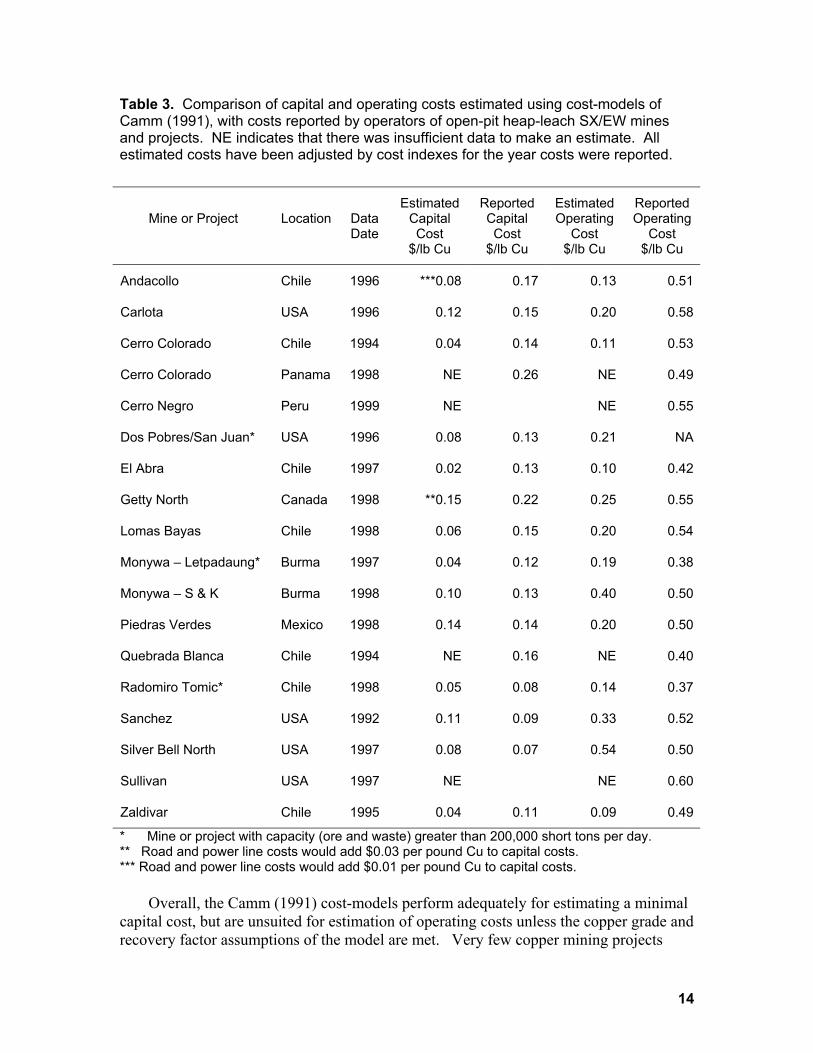
Camm’s (1991) equations (equations 5 through 8) were used to estimate capital and operating costs for each of the mines and projects in table 1 for which there are sufficient data. Results are presented in table 3 along with the reported values from table 1 for comparison. Note that capital and operating costs have been recalculated in terms of U.S. dollars per pound of copper. Capital costs do not include road and power line costs as information on infrastructure requirements could not be found for all mines and projects. Estimated road and power line costs for those mines and projects for which data was available were generally less than $0.005 per pound copper. Exceptions are noted in table 3. Three mines and projects in table 3 have mine capacities that exceed the validity range of the Camm (1991) large open-pit mine cost-model. Cost estimates for these mines and projects are extrapolations outside the valid range of the underlying cost model.

The Camm (1991) models consistently underestimate capital costs for mines and projects in South America and Asia. Estimated capital costs for North American mines and projects are fairly close to their reported values. These results are consistent with our observation that capital costs may be higher in South America due to much higher infrastructure costs and costs related to importation of capital goods.

Operating costs are underestimated, by as much as 80 percent, except in one instance. Given the weakness of the cost-model for heap-leach, SX-EW facilities, which assumes a copper grade of 0.4 percent copper and a recovery factor of 50 percent, and our inability to adjust the open-pit cost model for variable haulage distance, large deviations of estimated costs from reported costs are not unexpected. Consistent underestimation requires explanation, however. Note that almost all mines and projects in table 1 have copper grades significantly higher than 0.4 percent and recovery factors much higher than 50 percent. This would result in much more copper produced at a given mine capacity than would be recovered at the copper grade and recovery factor assumed by the cost-model. Under these circumstances, estimated costs would be diluted by the additional copper yielding a significant underestimate.

14

Table 3. Comparison of capital and operating costs estimated using cost-models of Camm (1991), with costs reported by operators of open-pit heap-leach SX/EW mines and projects. NE indicates that there was insufficient data to make an estimate. All estimated costs have been adjusted by cost indexes for the year costs were reported.

Mine or Project

Location

Data Date

Estimated Capital Cost

$/lb Cu

Reported Capital Cost

$/lb Cu

Estimated Operating

Cost $/lb Cu

Reported Operating

Cost $/lb Cu

Andacollo Chile 1996 ***0.08 0.17 0.13 0.51

Carlota USA 1996 0.12 0.15 0.20 0.58

Cerro Colorado Chile 1994 0.04 0.14 0.11 0.53

Cerro Colorado Panama 1998 NE 0.26 NE 0.49

Cerro Negro Peru 1999 NE NE 0.55

Dos Pobres/San Juan* USA 1996 0.08 0.13 0.21 NA

El Abra Chile 1997 0.02 0.13 0.10 0.42

Getty North Canada 1998 **0.15 0.22 0.25 0.55

Lomas Bayas Chile 1998 0.06 0.15 0.20 0.54

Monywa – Letpadaung* Burma 1997 0.04 0.12 0.19 0.38

Monywa – S & K Burma 1998 0.10 0.13 0.40 0.50

Piedras Verdes Mexico 1998 0.14 0.14 0.20 0.50

Quebrada Blanca Chile 1994 NE 0.16 NE 0.40

Radomiro Tomic* Chile 1998 0.05 0.08 0.14 0.37

Sanchez USA 1992 0.11 0.09 0.33 0.52

Silver Bell North USA 1997 0.08 0.07 0.54 0.50

Sullivan USA 1997 NE NE 0.60

Zaldivar Chile 1995 0.04 0.11 0.09 0.49

* Mine or project with capacity (ore and waste) greater than 200,000 short tons per day. ** Road and power line costs would add $0.03 per pound Cu to capital costs. *** Road and power line costs would add $0.01 per pound Cu to capital costs.

Overall, the Camm (1991) cost-models perform adequately for estimating a minimal capital cost, but are unsuited for estimation of operating costs unless the copper grade and recovery factor assumptions of the model are met. Very few copper mining projects

15

meet these grade (0.4 percent copper) and recovery factor (50 percent) assumptions, thus the operating cost model is of limited utility.

Application Example To illustrate application of these cost filters, we apply each filter to the Cochise

porphyry copper deposit, located north of the inactive Lavender open-pit copper mine at Bisbee, Warren mining district, Cochise County, Arizona. We estimate operating and capital costs for mining this deposit and determine if that mine will be profitable at a copper price of $0.85 per pound copper. This deposit is owned by Phelps Dodge Corp., who list the deposit as a leach resource in their recent annual filings with the Securities and Exchange Commission (Phelps Dodge, 2001). Phelps Dodge reports that the deposit contains 210 million short tons (191 million metric tons) of copper ore containing 0.40 percent copper (Phelps Dodge, 2001).

Phelps Dodge has not reported how much waste must be removed to mine the deposit or the results of any feasibility studies it may have performed. We will consider 5 cases, with waste to ore ratios of 0.5, 0.75, 1.0, 1.25, and 1.5 to 1 respectively. The copper grade of 0.4 percent is the same grade assumed by the Camm (1991) model for heap leach recovery of copper. Recall that this model also assumes a 50 percent recovery of copper. Phelps Dodge has not reported results of metallurgical testing of ore from the Cochise deposit.

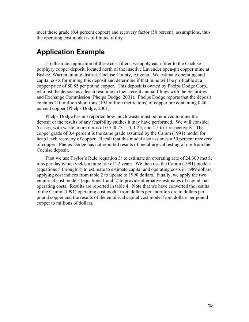
First we use Taylor’s Rule (equation 3) to estimate an operating rate of 24,300 metric tons per day which yields a mine life of 22 years. We then use the Camm (1991) models (equations 5 through 8) to estimate to estimate capital and operating costs in 1989 dollars, applying cost indices from table 2 to update to 1990 dollars. Finally, we apply the two empirical cost models (equations 1 and 2) to provide alternative estimates of capital and operating costs. Results are reported in table 4. Note that we have converted the results of the Camm (1991) operating cost model from dollars per short ton ore to dollars per pound copper and the results of the empirical capital cost model from dollars per pound copper to millions of dollars.

16

Table 4. Comparison of capital and operating costs estimated using empirical and Camm cost models.

Capital Cost (million dollars) Operating Cost (dollars per pound)

Waste:Ore Camm Model

Empirical Model Camm Model Empirical Model

0.50 54 117 0.70 0.54 0.75 62 134 0.76 0.54 1.00 70 150 0.83 0.54 1.25 78 165 0.90 0.53 1.50 86 181 0.96 0.53

To determine whether any of these scenarios is economic at a copper price of $0.85 per pound copper, we apply a simple net present value calculation with an initial outlay equal to estimated capital cost and net revenues at the end of each of 22 years calculated as gross revenue net of operating costs for the year. An interest rate of 10 percent is assumed. Note that this simple calculation does not take into account Federal and State income and severance taxes. Results are presented in table 5.

Table 5. Comparison of net present value calculations from results of Camm (1991), empirical, and recommended (mixed) cost models. The recommended (mixed) cost model uses the Camm (1991) capital cost model and the empirical operating cost model.

Net Present Value (million dollars) Waste:Ore Camm (1991)

Model Empirical Model Recommended

Model

0.50 -3 -11 53 0.75 -31 -28 44 1.00 -63 -44 36 1.25 -95 -55 32 1.50 -124 -71 24

The Camm (1991) and empirical models predict that the Cochise deposit will be uneconomic to mine at a copper price of $0.85 per pound whereas the recommended model predicts that the deposit will be economic to mine at that price. The Camm (1991) model, which has been shown to overestimate operating costs, estimates operating costs (table 4) which are close to the assumed price of copper. The empirical model, which has been shown to estimate higher capital costs than should obtain in the United States, estimates capital costs (table 4) which are much higher than those estimated by the Camm

17

model. The recommended model uses the capital cost model of Camm (1991) and the empirical operating cost model and yields results which are more credible for mining conditions in the United States. The recommended model (see Conclusions) predicts that the Cochise deposit would be economic to mine within the range of waste-to-ore stripping ratios considered. That Phelps Dodge continues to list the Cochise deposit as a resource, and has announced no plans to develop it as a mine, may reflect economic factors known to Phelps Dodge and unknown to the authors, or that Phelps Dodge has more profitable alternatives for developing new copper mines.

Conclusions Comprehensive prefeasibility studies performed by mining engineers generally

predict capital and operating costs to within 30 percent of the costs actually achieved when a mine is developed (Hoskins, 1986). The simple empirical capital and operating cost models presented in figures 1 and 2 are comparable in predictive performance. The Camm (1991) capital cost model performs well for domestic projects with limited infrastructure requirements, but underestimates capital costs substantially for foreign projects where infrastructure costs are very high. The Camm (1991) operating cost model is too restrictive in its assumptions to be useful.

Overall, the empirical cost model has the advantage of implicit consideration of infrastructure, remediation, and other costs not directly related to mining and processing. Unfortunately, because the empirical cost model is based largely on South American mines and projects, it will estimate capital costs that are higher than would obtain in the United States. The best solution is to use the Camm (1991) model for estimating capital costs and the empirical model for estimating operating costs.

References Cited Camm, Thomas W., 1991, Simplified cost models for prefeasibility mineral evaluations:

U.S. Bureau of Mines Information Circular 9298, 35 p. Hoskins, Jack, 1986, Foreword, in 1986 mineral industry costs; Northwest Mining

Association short course: Spokane, Washington, Northwest Mining Association, p. 1-4.

O’Hara, T. Alan and Suboleski, Stanley C., 1992, Costs and cost estimation, Chapter 6.3 in Hartman, Howard, L., senior ed., SME mining engineering handbook, 2nd edition: Littleton, Colorado, Society for Mining, Metallurgy, and Exploration, Inc., v. 1, p. 405-424.

Phelps Dodge, 2001, Form 10K; Annual report pursuant to section 13 or 15(d) of the Securities Exchange Act of 1934 for the fiscal year ended December 31, 2000: Phoenix, Arizona, Phelps Dodge Corp., 92 p.

Singer, Donald A., Menzie, W. David, and Long, Keith R., 1998, A simplified economic filter for open-pit gold-silver mining in the United States: U.S. Geological Survey Open-File Report 98-431, 10 p.

18

Singer, D.A., Menzie, W.D., and Long, K.R., 2000, A simplified economic filter for underground mining of massive sulfide deposits: U.S. Geological Survey Open-File Report 00-349, 20 p.

Smith, R. Craig, 1992, PREVAL; prefeasibility software program for evaluating mineral properties; version 1.01 user’s manual: U.S. Bureau of Mines Information Circular 9307, 45 p.

Stanley, Michael Claire, 1994, A quantitative estimation of the value of geoscience information in mineral exploration; optimal search sequences: Tucson, Arizona, University of Arizona, Doctoral dissertation, 398 p.

Taylor, H.K., 1986, Rates of working mines; a simple rule of thumb: Transactions of the Institution of Mining and Metallurgy, v. 95, section A, p. 203-204.

Tilton, John E., and Landsberg, Hans H., 1997, Innovation, productivity growth, and the survival of the U.S. copper industry: Washington, D.C., Resources for the Future, Discussion Paper 97-41, 32 p.