Brigham Young University Brigham Young University

BYU ScholarsArchive BYU ScholarsArchive

Theses and Dissertations

2007-03-17

A Simulation-Based Approach for Evaluating Gene Expression A Simulation-Based Approach for Evaluating Gene Expression

Analyses Analyses

Carly Ruth Pendleton Brigham Young University - Provo

Follow this and additional works at: https://scholarsarchive.byu.edu/etd

Part of the Statistics and Probability Commons

BYU ScholarsArchive Citation BYU ScholarsArchive Citation Pendleton, Carly Ruth, "A Simulation-Based Approach for Evaluating Gene Expression Analyses" (2007). Theses and Dissertations. 848. https://scholarsarchive.byu.edu/etd/848

This Thesis is brought to you for free and open access by BYU ScholarsArchive. It has been accepted for inclusion in Theses and Dissertations by an authorized administrator of BYU ScholarsArchive. For more information, please contact scholarsarchive@byu.edu, ellen_amatangelo@byu.edu.

A SIMULATION-BASED APPROACH FOR EVALUATING

GENE EXPRESSION ANALYSES

by

Carly R. Pendleton

A thesis submitted to the faculty of

Brigham Young University

in partial fulfillment of the requirements for the degree of

Master of Science

Department of Statistics

Brigham Young University

April 2007

BRIGHAM YOUNG UNIVERSITY

GRADUATE COMMITTEE APPROVAL

of a thesis submitted by

Carly R. Pendleton

This thesis has been read by each member of the following graduate committee andby majority vote has been found to be satisfactory.

Date Natalie J. Blades, Chair

Date Scott D. Grimshaw

Date William Christensen

BRIGHAM YOUNG UNIVERSITY

As chair of the candidate’s graduate committee, I have read the thesis of Carly R.Pendleton in its final form and have found that (1) its format, citations, and bibli-ographical style are consistent and acceptable and fulfill university and departmentstyle requirements; (2) its illustrative materials including figures, tables, and chartsare in place; and (3) the final manuscript is satisfactory to the graduate committeeand is ready for submission to the university library.

Date Natalie J. BladesChair, Graduate Committee

Accepted for the Department

Scott D. GrimshawGraduate Coordinator

Accepted for the College

Thomas W. SederbergAssociate Dean, College of Physical andMathematical Sciences

ABSTRACT

A SIMULATION-BASED APPROACH FOR EVALUATING

GENE EXPRESSION ANALYSES

Carly R. Pendleton

Department of Statistics

Master of Science

Microarrays enable biologists to measure differences in gene expression in thou-

sands of genes simultaneously. The data produced by microarrays present a statistical

challenge, one which has been met both by new modifications of existing methods

and by completely new approaches. One of the difficulties with a new approach to

microarray analysis is validating the method’s power and sensitivity. A simulation

study could provide such validation by simulating gene expression data and investi-

gating the method’s response to changes in the data; however, due to the complex

dependencies and interactions found in gene expression data, such a simulation would

be complicated and time consuming. This thesis proposes a way to simulate gene ex-

pression data and validate a method by borrowing information from existing data.

Analogous to the spike-in technique used to validate expression levels on an array,

this simulation-based approach will add a simulated gene with known features to

an existing data set. Analysis of this appended data set will reveal aspects of the

method’s sensitivity and power. The method and data on which this technique is

illustrated come from Storey et al. (2005).

ACKNOWLEDGEMENTS

I would like to thank those who have supported me throughout this thesis:

my husband, Jeff, for offering encouragement and devotion; my parents, for always

providing the opportunity to excel; Dr. Natalie Blades, for introducing me to the

world of microarrays; the BYU Statistics department faculty, for refusing to let me

be mediocre; and most importantly, my Heavenly Father, for blessing me with the

mind and strength to accomplish all.

CONTENTS

CHAPTER

1 Introduction 1

1.1 Basic Molecular Biology . . . . . . . . . . . . . . . . . . . . . . . . . 1

1.1.1 The Central Dogma . . . . . . . . . . . . . . . . . . . . . . . . 1

1.1.2 DNA and Replication . . . . . . . . . . . . . . . . . . . . . . . 3

1.1.3 RNA and Transcription . . . . . . . . . . . . . . . . . . . . . 8

1.1.4 Protein and Translation . . . . . . . . . . . . . . . . . . . . . 10

1.2 Microarrays . . . . . . . . . . . . . . . . . . . . . . . . . . . . . . . . 12

1.2.1 Studying Gene Expression . . . . . . . . . . . . . . . . . . . . 13

1.2.2 The Microarray Process . . . . . . . . . . . . . . . . . . . . . 15

1.2.3 Analysis Methods . . . . . . . . . . . . . . . . . . . . . . . . . 18

1.2.3.1 Preprocessing . . . . . . . . . . . . . . . . . . . . . . 18

1.2.3.2 Clustering Methods . . . . . . . . . . . . . . . . . . 20

1.2.3.3 Inference . . . . . . . . . . . . . . . . . . . . . . . . 25

1.2.3.4 Multiple Comparisons . . . . . . . . . . . . . . . . . 29

2 Review of Methods 31

2.1 A Modified F -statistic . . . . . . . . . . . . . . . . . . . . . . . . . . 31

2.2 A Dependent Correlation Matrix . . . . . . . . . . . . . . . . . . . . 33

2.3 A Robust Wald Statistic . . . . . . . . . . . . . . . . . . . . . . . . . 34

2.4 Guide Genes . . . . . . . . . . . . . . . . . . . . . . . . . . . . . . . . 34

2.5 Mixture Analysis . . . . . . . . . . . . . . . . . . . . . . . . . . . . . 35

2.6 Hidden Markov Models . . . . . . . . . . . . . . . . . . . . . . . . . . 36

2.7 Method Comparison and Evaluation . . . . . . . . . . . . . . . . . . 37

xi

3 Storey Method 38

3.1 Motivating Experiment and Objective . . . . . . . . . . . . . . . . . . 38

3.2 Detecting Differential Gene Expression . . . . . . . . . . . . . . . . . 39

3.2.1 Method Details . . . . . . . . . . . . . . . . . . . . . . . . . . 41

4 Simulation Study 44

4.1 Simulating Gene Expression Data . . . . . . . . . . . . . . . . . . . . 44

4.2 Varying Features of the Data . . . . . . . . . . . . . . . . . . . . . . 47

4.2.1 Choice of µ . . . . . . . . . . . . . . . . . . . . . . . . . . . . 48

4.2.2 The Effect of ρ . . . . . . . . . . . . . . . . . . . . . . . . . . 53

4.2.3 The Effect of σ2 . . . . . . . . . . . . . . . . . . . . . . . . . . 54

4.2.4 Attenuation of Difference Between Control and Treated Arrays 57

5 Evaluating Gene Expression Analyses Through Simulation Studies 62

APPENDIX

A Source Code for Storey et al. method 68

B Tabular Results from Simulation Study 77

xii

TABLES

Table

1.1 Amino acid coding chart . . . . . . . . . . . . . . . . . . . . . . . . . 11

1.2 Number of errors committed when testing m null hypotheses . . . . . 29

B.1 Results of first attenuation simulation. . . . . . . . . . . . . . . . . . 77

B.2 Results of second attenuation simulation. . . . . . . . . . . . . . . . . 78

B.3 Results of simulation with σ2 = 25, 000. . . . . . . . . . . . . . . . . . 78

B.4 Results of simulation with σ2 = 250, 000. . . . . . . . . . . . . . . . . 79

B.5 Results of simulation with σ2 = 2, 500, 000. . . . . . . . . . . . . . . . 79

B.6 Results of first attenuation simulation (average rankings). . . . . . . . 80

B.7 Results of second attenuation simulation (average rankings). . . . . . 80

B.8 Results of simulation with σ2 = 25, 000 (average rankings). . . . . . . 81

B.9 Results of simulation with σ2 = 250, 000 (average rankings). . . . . . 81

B.10 Results of simulation with σ2 = 2, 500, 000 (average rankings). . . . . 82

xiii

FIGURES

Figure

1.1 The central dogma of biology . . . . . . . . . . . . . . . . . . . . . . 3

1.2 The four DNA nucleotides . . . . . . . . . . . . . . . . . . . . . . . . 4

1.3 Deoxyribonucleic acid . . . . . . . . . . . . . . . . . . . . . . . . . . . 5

1.4 Deoxyribonucleic acid—molecular structure . . . . . . . . . . . . . . 5

1.5 Base pairings in DNA . . . . . . . . . . . . . . . . . . . . . . . . . . . 6

1.6 The replication process . . . . . . . . . . . . . . . . . . . . . . . . . . 7

1.7 The transcription process . . . . . . . . . . . . . . . . . . . . . . . . . 9

1.8 Reading frames . . . . . . . . . . . . . . . . . . . . . . . . . . . . . . 11

1.9 A Northern blot . . . . . . . . . . . . . . . . . . . . . . . . . . . . . . 14

1.10 Experimental design using microarrays . . . . . . . . . . . . . . . . . 16

1.11 Scanned image of a microarray . . . . . . . . . . . . . . . . . . . . . . 17

1.12 A microarray printer . . . . . . . . . . . . . . . . . . . . . . . . . . . 19

1.13 MA plots . . . . . . . . . . . . . . . . . . . . . . . . . . . . . . . . . 20

1.14 Boxplots of log-ratios by print-tip group . . . . . . . . . . . . . . . . 21

1.15 An example of hierarchical clustering from Eisen et al. (1998) . . . . 23

1.16 The SOM process (Tamayo et al. 1999) . . . . . . . . . . . . . . . . . 24

2.1 Null and alternative models fit to endotoxin data . . . . . . . . . . . 32

3.1 Distribution of p-values for endotoxin data . . . . . . . . . . . . . . . 42

4.1 A histogram of estimates of ρ . . . . . . . . . . . . . . . . . . . . . . 48

4.2 A histogram of estimates of the variance . . . . . . . . . . . . . . . . 49

4.3 Mean vectors used to simulate genes . . . . . . . . . . . . . . . . . . 50

4.4 Power curves showing effect of µ, σ2, and ρ and vector on simulated

genes . . . . . . . . . . . . . . . . . . . . . . . . . . . . . . . . . . . . 52

xiv

4.5 First attenuation simulation . . . . . . . . . . . . . . . . . . . . . . . 55

4.6 Boxplots of ranked genes from first attenuation simulation . . . . . . 56

4.7 Second attenuation simulation . . . . . . . . . . . . . . . . . . . . . . 59

4.8 Boxplots of ranked genes from second attenuation simulation . . . . . 61

xv

1. INTRODUCTION

The biological systems that create and maintain life are intensely complex. They

are difficult to study because many interdependent biochemical systems are present.

Many of the seminal experiments in biology involved entire organisms and were con-

sidered “black boxes”—the organism itself could be observed but the components

that determine the organism’s functions remain a mystery. Over the past century,

biologists have been slowly breaking the black boxes into smaller and smaller pieces,

eventually arriving at the molecular level. Duplicating “life” requires understand-

ing how thousands of these black boxes interact. Studying bits of real life requires

monitoring hundreds and even thousands of chemical reactions that mostly occur

simultaneously in a vast network of checks and balances. Microarrays are revolution-

izing biology research by allowing researchers to design and analyze experiments that

do just that.

1.1 Basic Molecular Biology

Microarrays were designed as a response to the need to analyze gene expression

data. Consequently, a basic understanding of molecular biology becomes useful in

understanding how the data are collected and how they should be handled. This

section will introduce the main concepts of molecular biology and how they relate to

microarrays.

1.1.1 The Central Dogma

To understand the technology and strategy behind microarrays, it is important

to first understand the central dogma—the organizing principle behind molecular

biology. James Watson and Francis Crick, famous for their discovery of DNA’s double

1

helix structure, proposed the idea of the central dogma in 1958. Originally more of an

afterthought than a core theory, Watson’s first representation of the central dogma

was no more than a note on a scrap of paper:

The idea of genes being immortal smelled right, and so on my wallabove my desk I taped up a paper sheet saying DNA→RNA→protein.The arrows did not signify chemical transformations, but instead ex-pressed the transfer of genetic information from the sequence of nu-cleotides in DNA molecules to the sequences of amino acids in pro-teins.

—Watson (2001)

The term “dogma,” attributed to Crick, has often been criticized for its strict

connotation. Crick intended it to be used with a looser definition:

[An associate] pointed out to me that I did not appear to understandthe correct use of the word dogma, which is a belief that cannot bedoubted. . . . I used the word the way I myself thought about it, not asmost of the world does, and simply applied it to a grand hypothesisthat, however plausible, had little direct experimental support.

—Crick (1988)

In the fifty years since the proposal of the central dogma, substantial evidence

has been found in its favor and even the most rigorous definition of dogma is felt to be

appropriate. When Watson and Crick submitted a paper to Nature in 1953 claiming

to know the structure of DNA, the paper “was not peer-reviewed by Nature. . . the

paper could not have been refereed: its correctness is self-evident. No referee working

in the field . . . could have kept his mouth shut once he saw the structure . . . ” (Maddox

2003).

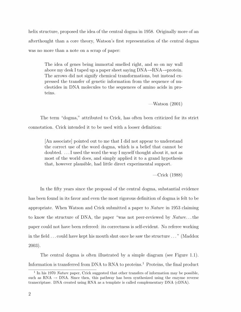
The central dogma is often illustrated by a simple diagram (see Figure 1.1).

Information is transferred from DNA to RNA to proteins.1 Proteins, the final product

1 In his 1970 Nature paper, Crick suggested that other transfers of information may be possible,such as RNA → DNA. Since then, this pathway has been synthesized using the enzyme reversetranscriptase. DNA created using RNA as a template is called complementary DNA (cDNA).

2

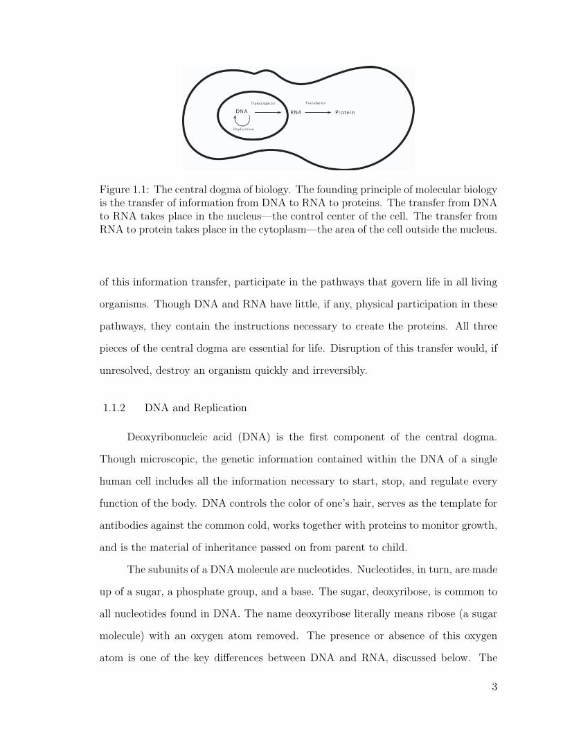
Figure 1.1: The central dogma of biology. The founding principle of molecular biologyis the transfer of information from DNA to RNA to proteins. The transfer from DNAto RNA takes place in the nucleus—the control center of the cell. The transfer fromRNA to protein takes place in the cytoplasm—the area of the cell outside the nucleus.

of this information transfer, participate in the pathways that govern life in all living

organisms. Though DNA and RNA have little, if any, physical participation in these

pathways, they contain the instructions necessary to create the proteins. All three

pieces of the central dogma are essential for life. Disruption of this transfer would, if

unresolved, destroy an organism quickly and irreversibly.

1.1.2 DNA and Replication

Deoxyribonucleic acid (DNA) is the first component of the central dogma.

Though microscopic, the genetic information contained within the DNA of a single

human cell includes all the information necessary to start, stop, and regulate every

function of the body. DNA controls the color of one’s hair, serves as the template for

antibodies against the common cold, works together with proteins to monitor growth,

and is the material of inheritance passed on from parent to child.

The subunits of a DNA molecule are nucleotides. Nucleotides, in turn, are made

up of a sugar, a phosphate group, and a base. The sugar, deoxyribose, is common to

all nucleotides found in DNA. The name deoxyribose literally means ribose (a sugar

molecule) with an oxygen atom removed. The presence or absence of this oxygen

atom is one of the key differences between DNA and RNA, discussed below. The

3

phosphate group also has the same basic structure for all nucleotides and serves as

the connector between nucleotides. The base, however, has four varieties: adenine

(A), guanine (G), cytosine (C), and thymine (T).

Figure 1.2: The four DNA nucleotides. All nucleotides have a pentagonal carbon ring(bottom left of each nucleotide). The difference between purines and pyrimidines liesin the ring(s) connected to the base ring. Purines have two rings (top right of purines)while pyrimidines have only one ring (top right of pyrimidines).

Figure 1.2 displays the atomic structure of the four bases. Adenine and guanine

are composed of two fused rings; these are called purines. Cytosine and thymine have

only one ring; these are pyrimidines. Another pyrimidine, uracil, is not found in

DNA but plays an important role in RNA. Through various combinations of these

four bases, infinite sequences are possible, allowing for the remarkable versatility of

DNA; a sequence of only 10 bases would allow 410 or 1,048,576 possible sequences.

Considering that the human genome—the entire set of DNA required for a living

organism—contains over 3 billion bases, it is no wonder that no two organisms are

alike.

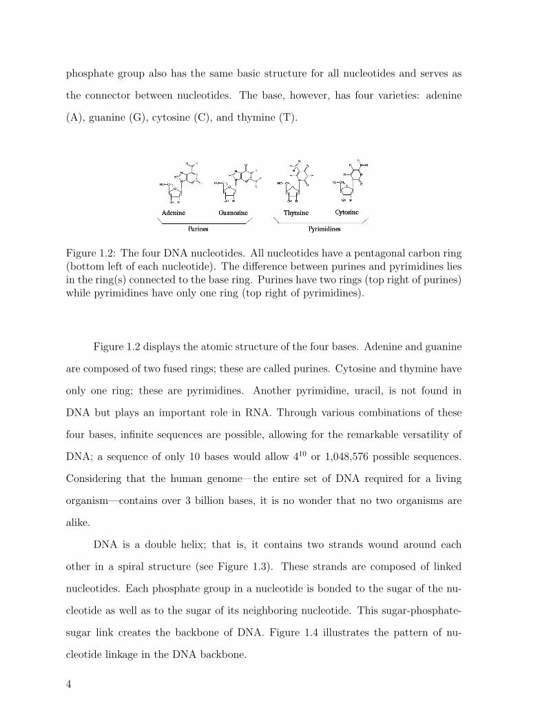
DNA is a double helix; that is, it contains two strands wound around each

other in a spiral structure (see Figure 1.3). These strands are composed of linked

nucleotides. Each phosphate group in a nucleotide is bonded to the sugar of the nu-

cleotide as well as to the sugar of its neighboring nucleotide. This sugar-phosphate-

sugar link creates the backbone of DNA. Figure 1.4 illustrates the pattern of nu-

cleotide linkage in the DNA backbone.

4

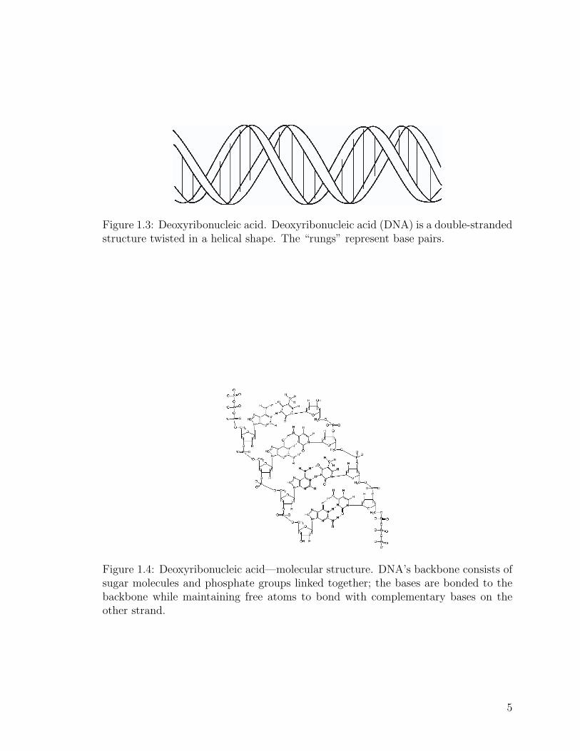
Figure 1.3: Deoxyribonucleic acid. Deoxyribonucleic acid (DNA) is a double-strandedstructure twisted in a helical shape. The “rungs” represent base pairs.

Figure 1.4: Deoxyribonucleic acid—molecular structure. DNA’s backbone consists ofsugar molecules and phosphate groups linked together; the bases are bonded to thebackbone while maintaining free atoms to bond with complementary bases on theother strand.

5

The sugar and the phosphate group are used to connect the nucleotides of a

single strand, while the bases of the two strands of DNA pair with each other. Each

pair of bases forms a link between the two strands of DNA, much like the rungs of a

ladder connect its sides. Purines are bulkier than pyrimidines because they have two

rings versus one ring (see Figure 1.2). Therefore, a purine must pair with a pyrimidine

to preserve a uniform distance between the two strands.2 Slight differences among

the bases dictate which base pairs are possible: adenine pairs only with thymine and

cytosine pairs only with guanine. In an adenine-thymine pair, two hydrogen bonds

are formed; in a guanine-cytosine pair, three hydrogen bonds are formed. The bonds

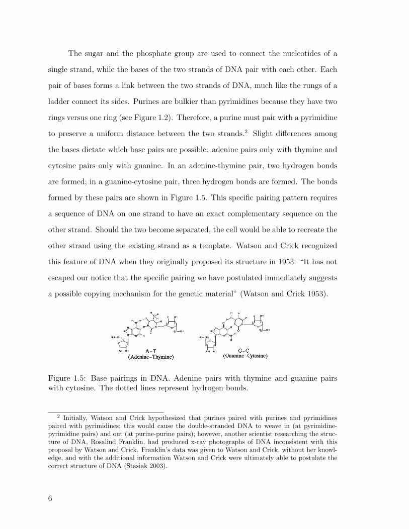
formed by these pairs are shown in Figure 1.5. This specific pairing pattern requires

a sequence of DNA on one strand to have an exact complementary sequence on the

other strand. Should the two become separated, the cell would be able to recreate the

other strand using the existing strand as a template. Watson and Crick recognized

this feature of DNA when they originally proposed its structure in 1953: “It has not

escaped our notice that the specific pairing we have postulated immediately suggests

a possible copying mechanism for the genetic material” (Watson and Crick 1953).

Figure 1.5: Base pairings in DNA. Adenine pairs with thymine and guanine pairswith cytosine. The dotted lines represent hydrogen bonds.

2 Initially, Watson and Crick hypothesized that purines paired with purines and pyrimidinespaired with pyrimidines; this would cause the double-stranded DNA to weave in (at pyrimidine-pyrimidine pairs) and out (at purine-purine pairs); however, another scientist researching the struc-ture of DNA, Rosalind Franklin, had produced x-ray photographs of DNA inconsistent with thisproposal by Watson and Crick. Franklin’s data was given to Watson and Crick, without her knowl-edge, and with the additional information Watson and Crick were ultimately able to postulate thecorrect structure of DNA (Stasiak 2003).

6

For cell growth and maintenance, DNA must replicate itself periodically. As

cells grow and divide, they pass on a copy of their DNA to their offspring, or daughter

cells. The complementary pairing of bases provides for exact replication of a strand of

DNA. In this way, a cell can make duplicates of its DNA and distribute the duplicates

as it divides, giving rise to cells that are identical in every way to the original cell.

The replication process begins with two parent strands separating by breaking

the bonds between bases. Once a portion of the strands are separated, mechanisms

within the cell identify which base pair is needed to match the now unpaired base on

the parent strand. A new strand is built by selecting the appropriate nucleotide to

match the parent strand and forming new bonds between the bases. This process of

unwinding the strands, finding a new base, and forming new bonds continues along

the entire length of the DNA molecule. When the process is completed, two double-

stranded daughter DNA molecules are generated, exact replicates of the parent strand.

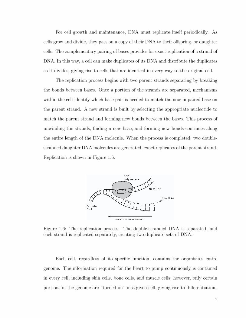
Replication is shown in Figure 1.6.

Figure 1.6: The replication process. The double-stranded DNA is separated, andeach strand is replicated separately, creating two duplicate sets of DNA.

Each cell, regardless of its specific function, contains the organism’s entire

genome. The information required for the heart to pump continuously is contained

in every cell, including skin cells, bone cells, and muscle cells; however, only certain

portions of the genome are “turned on” in a given cell, giving rise to differentiation.

7

1.1.3 RNA and Transcription

The second component of the central dogma is ribonucleic acid (RNA). RNA

is structurally very similar to DNA; both are nucleic acids—chains of nucleotides.

Despite these similarities, there are several key differences between RNA and DNA:

RNA is single-stranded, whereas DNA is always double-stranded; RNA uses a slightly

different sugar, ribose, in its structure; and RNA uses the pyrimidine uracil (U) in

place of thymine.

The central dogma suggests that the information in DNA is copied into RNA.

Transcription is the process in which a strand of DNA is used as a template to create a

new strand of RNA. This process is similar to DNA replication, but in replication, the

entire genome is replicated. In transcription, only the portions of DNA that contain

the information necessary for the functions of a particular cell are transcribed into

RNA. For example, in epidermal cells, the DNA that codes for melanin—the pigment

that gives skin color—will be transcribed, but the DNA that codes for insulin—a

hormone that aids in sugar breakdown—will not be transcribed. RNA is usually

found in short strands, each containing the code for a single gene, a portion of DNA

that codes for a functional protein (Lodish et al. 2000). Once again, it is important

to note that the original sequence of bases found on a parent DNA strand is preserved

throughout replication and transcription.

Transcription takes place in three steps: initiation, elongation, and termination

(see Figure 1.7). In all three steps a protein called RNA polymerase directs the

process. Transcription is initiated when the polymerase recognizes a region of DNA

called a promoter. The polymerase attaches to the RNA at the promoter and begins

separating the DNA strands. Just “downstream” of the promoter is the start site

where the polymerase begins building the RNA chain. Once a few nucleotides have

been joined, elongation begins. The polymerase leaves the promoter and moves down

the DNA strand, adding corresponding nucleotides to the growing RNA chain. The

8

newly created RNA does not stay bound to the DNA, rather, it detaches a few bases

behind the polymerase. The separated DNA strands rewind behind the polymerase

as the portion is transcribed. Eventually the polymerase approaches a region of DNA

called the terminator. The terminator signals to the polymerase to release the DNA

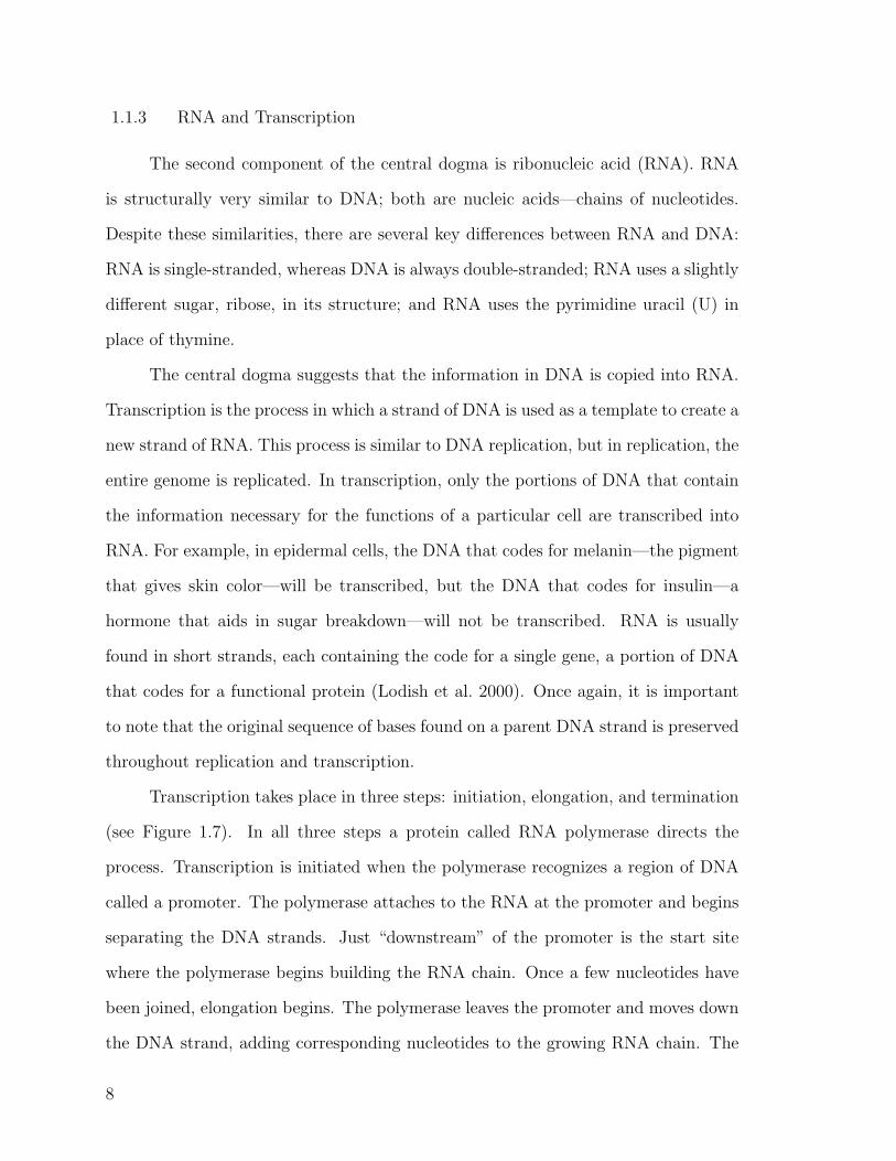
template and the newly created RNA strand. At this point, transcription is complete.

Figure 1.7: The transcription process. RNA polymerase builds a chain of RNAcomplementary to the template DNA.

Although it does not occur naturally within the cell, DNA can be created from

RNA. This process, known as reverse transcription, uses the enzyme reverse tran-

scriptase from retroviruses. Reverse transcriptase produces a strand of DNA com-

plementary to a strand of RNA (reversing the usual procedure) (Lodish et al. 2000).

RNA includes the code for only the genes which will be activated in a particular cell;

therefore, reverse transcription provides the DNA for active genes. If the DNA were

extracted directly from the cell and not created via reverse transcription, it would

contain the code for all genes, not just those genes being synthesized. By reversing

the transcription process and creating new DNA from RNA (called cDNA), a copy of

DNA can be obtained that excludes all unused material. cDNA is an important tool

in implementing the methods of microarrays.

9

1.1.4 Protein and Translation

Proteins are the final element of the central dogma. While DNA and RNA are

strings of nucleotides, proteins are strings of amino acids. Just as different combi-

nations of the four nucleotides allow infinite possibilities in DNA, various sequences

of twenty amino acids provide for great diversity among proteins. At the core of the

central dogma is the idea that the code found in DNA is passed through RNA to

create proteins. From DNA to RNA, the code is preserved base for base; from RNA

to protein, the sequence is “translated” from nucleotides into amino acids.

Much like translating between two languages, translation in the cell converts

the RNA sequence into an amino acid sequence. Every three base pairs in either RNA

or DNA make up a codon. Each codon codes for a single amino acid (see Table 1.1).

The cell machinery scans RNA, picking off one codon at a time and finding the

corresponding amino acid. Once a chain of amino acids has been connected, it is

referred to as a polypeptide, or protein. Proteins are the products that perform tasks

within the cell.

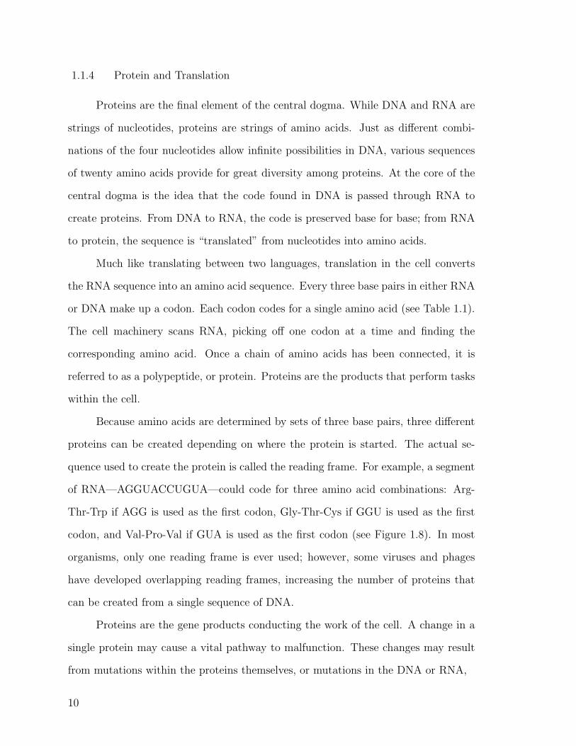
Because amino acids are determined by sets of three base pairs, three different

proteins can be created depending on where the protein is started. The actual se-

quence used to create the protein is called the reading frame. For example, a segment

of RNA—AGGUACCUGUA—could code for three amino acid combinations: Arg-

Thr-Trp if AGG is used as the first codon, Gly-Thr-Cys if GGU is used as the first

codon, and Val-Pro-Val if GUA is used as the first codon (see Figure 1.8). In most

organisms, only one reading frame is ever used; however, some viruses and phages

have developed overlapping reading frames, increasing the number of proteins that

can be created from a single sequence of DNA.

Proteins are the gene products conducting the work of the cell. A change in a

single protein may cause a vital pathway to malfunction. These changes may result

from mutations within the proteins themselves, or mutations in the DNA or RNA,

10

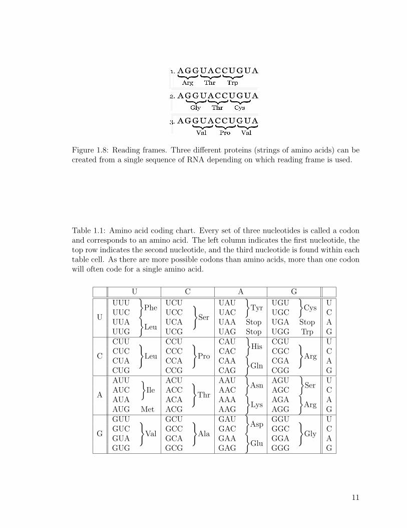
Figure 1.8: Reading frames. Three different proteins (strings of amino acids) can becreated from a single sequence of RNA depending on which reading frame is used.

Table 1.1: Amino acid coding chart. Every set of three nucleotides is called a codonand corresponds to an amino acid. The left column indicates the first nucleotide, thetop row indicates the second nucleotide, and the third nucleotide is found within eachtable cell. As there are more possible codons than amino acids, more than one codonwill often code for a single amino acid.

U C A G

U

UUU}

PheUCU }

Ser

UAU}

TyrUGU

}Cys

UUUC UCC UAC UGC CUUA

}Leu

UCA UAA Stop UGA Stop AUUG UCG UAG Stop UGG Trp G

C

CUU }Leu

CCU }Pro

CAU}

HisCGU }

Arg

UCUC CCC CAC CGC CCUA CCA CAA

}Gln

CGA ACUG CCG CAG CGG G

A

AUU }Ile

ACU }Thr

AAU}

AsnAGU

}Ser

UAUC ACC AAC AGC CAUA ACA AAA

}Lys

AGA}

ArgA

AUG Met ACG AAG AGG G

G

GUU }Val

GCU }Ala

GAU}

AspGGU }

Gly

UGUC GCC GAC GGC CGUA GCA GAA

}Glu

GGA AGUG GCG GAG GGG G

11

disrupting the code that would eventually be translated into protein. For example,

sickle-cell disease is a result of a single base change from adenine to thymine. Although

only one base is changed, the corresponding amino acid is also changed, causing the

protein to be altered. This disease causes those who have this mutation to have

sickle-shaped red blood cells. Under certain conditions, these blood cells will burst,

causing potentially fatal anemia.

To investigate which proteins are created in a cell, the proteins can be cataloged

or the RNA coding for the proteins in the cell can be examined. With thousands of

proteins present in a cell at any given time, extracting and identifying the proteins in

a cell is a drawn-out and tedious process. Extracting RNA is more practical. RNA

is a much smaller molecule than a protein, yet it still contains all the information

about the cell. Because of these features, RNA is a surrogate measure of the protein

activity in an organism and is often used in gene expression studies.

1.2 Microarrays

The ability to measure differences in gene expression has been a goal of biologists

for many years. Until recently, however, this goal has been difficult to attain. With

thousands of genes in a living organism, the time it would take to extract individual

genes and compare them on a normalized scale is daunting. In the past, scientists

have worked around this problem by examining a few genes at a time. Without the

ability to compare expression levels of thousands of genes, pathways could not be

identified, the expression of important genes could be overlooked, and progress could

only be made in very small steps.

With the establishment of the Human Genome Organization in 1989, the de-

mand for a method to measure differential gene expression increased greatly. Within

ten years, “researchers [had] catalogued more than 1.1 million expressed seqence

tagged sites (ESTs), corresponding with 52,907 unique human genes” (Duggan et al.

12

1999). However, the function of the majority of these genes remained unknown. In

response to the desire to identify the expression and regulation of sequenced genes,

the microarray was developed. Though only the size of a microscope slide, microar-

rays are capable of comparing up to 100,000 genes simultaneously. At first, the arrays

could only be used sparingly, as each chip cost about $1,000,000 to create (Muller and

Roder 2006, p.1). Now, lowered costs have increased the popularity of microarrays.

The name is well suited to the method, as “micro” means small and “array” refers

to an impressively large assembly. Since their development, microarrays have rapidly

become a widely used tool. In just the past ten years, over 30,000 articles have been

published concerning microarrays and microarray studies.

1.2.1 Studying Gene Expression

Prior to the introduction of the microarray, several methods existed to iden-

tify the function of a gene. Though each has proved inefficient in assessing several

thousand genes at once, they are useful when working with smaller numbers of genes.

Most of the methods for studying gene expression at the nucleic acid level utilize

the phenomenon of hybridization. Hybridization is the ability of single-stranded DNA

or RNA to bond with another single strand to form a double helix. This will only

occur when the two strands are complementary in their base pair pattern; that is, the

bases of one strand pair with the bases of the other strand along their entire length.

Northern blots is one technique that uses hybridization to measure gene activity.

The Northern blot technique collects RNA from the organism of interest. The

sample containing the RNA is inserted into a gel, similar to a thin sheet of jello. An

electric current draws the sample through the gel, separating the RNA based on size.

The RNA is then “blotted,” or transferred, onto a filter through diffusion. cDNA

from a gene of interest is labeled with a fluorescent or radioactive tag. The labeled

cDNA is then hybridized to the RNA on the filter. If the complementary RNA is

13

present, the cDNA will bind to it, forming a double helix. If the RNA is not present,

the cDNA will not hybridize and will be washed off the filter. When the filter is

passed through the appropriate steps to visualize the labeled cDNA, it becomes easy

to see whether the gene is present in the sample and relative amounts of the gene;

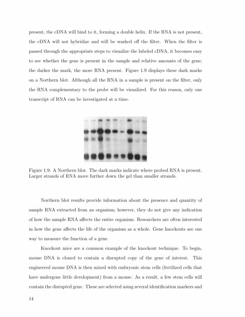
the darker the mark, the more RNA present. Figure 1.9 displays these dark marks

on a Northern blot. Although all the RNA in a sample is present on the filter, only

the RNA complementary to the probe will be visualized. For this reason, only one

transcript of RNA can be investigated at a time.

Figure 1.9: A Northern blot. The dark marks indicate where probed RNA is present.Larger strands of RNA move further down the gel than smaller strands.

Northern blot results provide information about the presence and quantity of

sample RNA extracted from an organism; however, they do not give any indication

of how the sample RNA affects the entire organism. Researchers are often interested

in how the gene affects the life of the organism as a whole. Gene knockouts are one

way to measure the function of a gene.

Knockout mice are a common example of the knockout technique. To begin,

mouse DNA is cloned to contain a disrupted copy of the gene of interest. This

engineered mouse DNA is then mixed with embryonic stem cells (fertilized cells that

have undergone little development) from a mouse. As a result, a few stem cells will

contain the disrupted gene. These are selected using several identification markers and

14

then inserted into a surrogate mother where they finish development. The surrogate

mother will give birth to mice with a mutant copy of the gene. These mice can be

observed to see the effect this gene has over their lifetime.

Both Northern blots and knockout mice are useful techniques when examin-

ing a single gene; however, a separate blot or knockout mouse must be created for

each gene of interest. Knockout organisms have the potential to inactivate three or

more genes at a time, but this number is limited by available markers (Mortensen

1993). Should the interest lie in a large number of genes, or if a study is largely

exploratory, Northern blots and knockouts are inadequate. The Complex Trait Con-

sortium project uses an eight-way cross of inbred mice lines to generate great genetic

diversity available for study; however, this method requires great quantities of mice

and is limited computationally and statistically (Williams et al. 2002). A study aided

by microarrays can overcome many of these limitations.

1.2.2 The Microarray Process

At first glance, a cDNA microarray looks very much like an ordinary microscope

slide. A closer look, however, will reveal thousands of tiny spots arranged in a rect-

angular grid. Each spot contains a piece of cDNA from a given organism’s genome.

A single microarray may contain an entire genome.

cDNA microarrays are constructed using replicated cDNA clones and precise

printing machinery. Again, cDNA is DNA created using RNA as a template. The

cDNA are replicated by polymerase chain reaction (PCR), a process that can amplify

one double-stranded segment of DNA into thousands of segments in a relatively short

period of time. Each replicated sample is contained in a well; each well holds thou-

sands of copies of the sample. The wells are arranged in grids, ready to be dipped

into and printed on the array.

When the array is complete, nearly 20,000 spots have been meticulously printed

15

onto the small slide. Each dot is not necessarily unique; common practice places the

same sample in different locations on the slide to control for error in array location.

Meanwhile, in the lab, the samples, or targets, are prepared to react with the

array. Each microarray is capable of comparing two targets. The selection of these

two targets depends on experimental design. For example, an experimenter may want

to use a control subject for the first target and a treated subject for a second target.

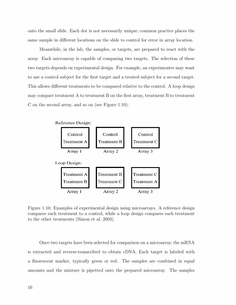
This allows different treatments to be compared relative to the control. A loop design

may compare treatment A to treatment B on the first array, treatment B to treatment

C on the second array, and so on (see Figure 1.10).

Figure 1.10: Examples of experimental design using microarrays. A reference designcompares each treatment to a control, while a loop design compares each treatmentto the other treatments (Simon et al. 2003).

Once two targets have been selected for comparison on a microarray, the mRNA

is extracted and reverse-transcribed to obtain cDNA. Each target is labeled with

a fluorescent marker, typically green or red. The samples are combined in equal

amounts and the mixture is pipetted onto the prepared microarray. The samples

16

hybridize to the probes on the array.

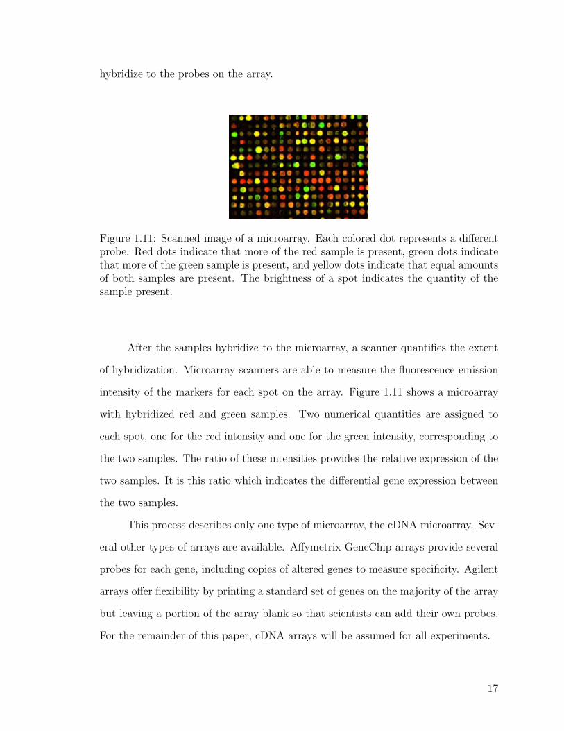
Figure 1.11: Scanned image of a microarray. Each colored dot represents a differentprobe. Red dots indicate that more of the red sample is present, green dots indicatethat more of the green sample is present, and yellow dots indicate that equal amountsof both samples are present. The brightness of a spot indicates the quantity of thesample present.

After the samples hybridize to the microarray, a scanner quantifies the extent

of hybridization. Microarray scanners are able to measure the fluorescence emission

intensity of the markers for each spot on the array. Figure 1.11 shows a microarray

with hybridized red and green samples. Two numerical quantities are assigned to

each spot, one for the red intensity and one for the green intensity, corresponding to

the two samples. The ratio of these intensities provides the relative expression of the

two samples. It is this ratio which indicates the differential gene expression between

the two samples.

This process describes only one type of microarray, the cDNA microarray. Sev-

eral other types of arrays are available. Affymetrix GeneChip arrays provide several

probes for each gene, including copies of altered genes to measure specificity. Agilent

arrays offer flexibility by printing a standard set of genes on the majority of the array

but leaving a portion of the array blank so that scientists can add their own probes.

For the remainder of this paper, cDNA arrays will be assumed for all experiments.

17

1.2.3 Analysis Methods

Most microarray analysis methods started as ad hoc ideas and have evolved into

theoretically sophisticated techniques. The methods described here are among those

generally accepted for data involving independent microarray data.

1.2.3.1 Preprocessing

Raw microarray data is rarely ready for immediate analysis. The human ele-

ment of creating microarrays often introduces irregularities in the data. Variation in

the data introduced by sources other than those factors being studied must be ac-

counted for in order for the analysis to be useful. Preprocessing techniques attempt

to standardize microarray data so that the analysis results can be compared.

First, numeric data must be extracted from the microarray image. The in-

tensity of each scanned pixel is collected; image analysis software categorizes each

pixel in the image as belonging to the sample or to the slide (foreground or back-

ground, respectively). The data includes some background noise usually resulting

from the scanning process. To account for this noise, image processing software will

subtract the background value from the intensity measurement. This technique can

be problematic because it introduces additional variability in the measurement. Some

methods recommend avoiding background subtraction if it does not seem necessary

(Parmigiani et al. 2003, p.14).

Several sources of variation introduce artificial differences among arrays. These

sources include unequal sample preparation, irregularities in the printing machinery,

and an uneven distribution of the sample on the array. Normalization of the data is

necessary in order to compare data across arrays.

One source of variation that requires normalization is the printing machinery.

The printing machinery consists of a print-head containing a number of print-tips.

Figure 1.12 shows a microarray printer. Each print-tip has a tiny hole that enables

18

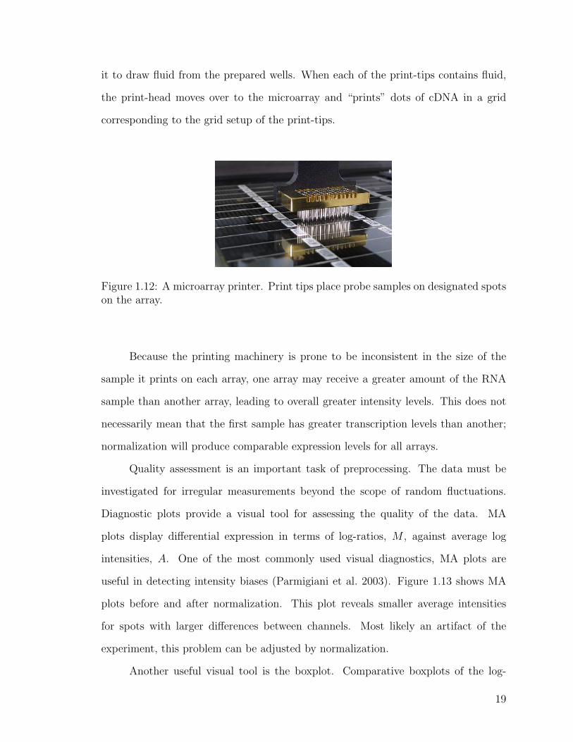
it to draw fluid from the prepared wells. When each of the print-tips contains fluid,

the print-head moves over to the microarray and “prints” dots of cDNA in a grid

corresponding to the grid setup of the print-tips.

Figure 1.12: A microarray printer. Print tips place probe samples on designated spotson the array.

Because the printing machinery is prone to be inconsistent in the size of the

sample it prints on each array, one array may receive a greater amount of the RNA

sample than another array, leading to overall greater intensity levels. This does not

necessarily mean that the first sample has greater transcription levels than another;

normalization will produce comparable expression levels for all arrays.

Quality assessment is an important task of preprocessing. The data must be

investigated for irregular measurements beyond the scope of random fluctuations.

Diagnostic plots provide a visual tool for assessing the quality of the data. MA

plots display differential expression in terms of log-ratios, M , against average log

intensities, A. One of the most commonly used visual diagnostics, MA plots are

useful in detecting intensity biases (Parmigiani et al. 2003). Figure 1.13 shows MA

plots before and after normalization. This plot reveals smaller average intensities

for spots with larger differences between channels. Most likely an artifact of the

experiment, this problem can be adjusted by normalization.

Another useful visual tool is the boxplot. Comparative boxplots of the log-

19

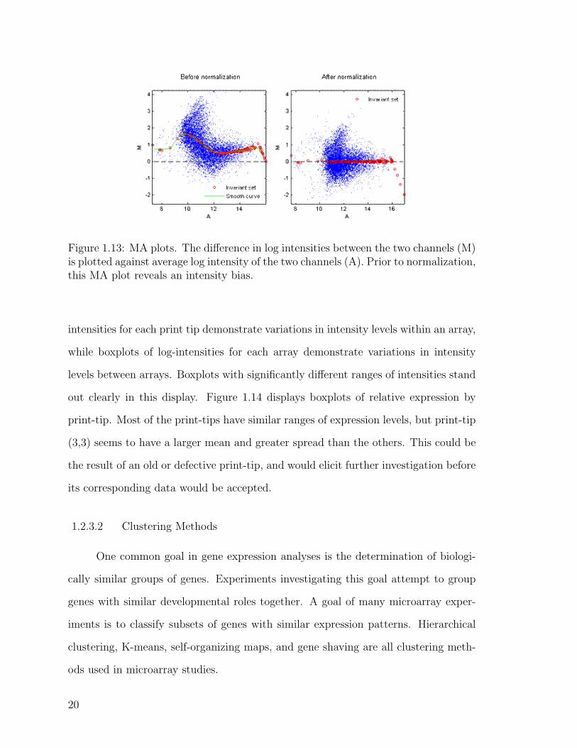
Figure 1.13: MA plots. The difference in log intensities between the two channels (M)is plotted against average log intensity of the two channels (A). Prior to normalization,this MA plot reveals an intensity bias.

intensities for each print tip demonstrate variations in intensity levels within an array,

while boxplots of log-intensities for each array demonstrate variations in intensity

levels between arrays. Boxplots with significantly different ranges of intensities stand

out clearly in this display. Figure 1.14 displays boxplots of relative expression by

print-tip. Most of the print-tips have similar ranges of expression levels, but print-tip

(3,3) seems to have a larger mean and greater spread than the others. This could be

the result of an old or defective print-tip, and would elicit further investigation before

its corresponding data would be accepted.

1.2.3.2 Clustering Methods

One common goal in gene expression analyses is the determination of biologi-

cally similar groups of genes. Experiments investigating this goal attempt to group

genes with similar developmental roles together. A goal of many microarray exper-

iments is to classify subsets of genes with similar expression patterns. Hierarchical

clustering, K-means, self-organizing maps, and gene shaving are all clustering meth-

ods used in microarray studies.

20

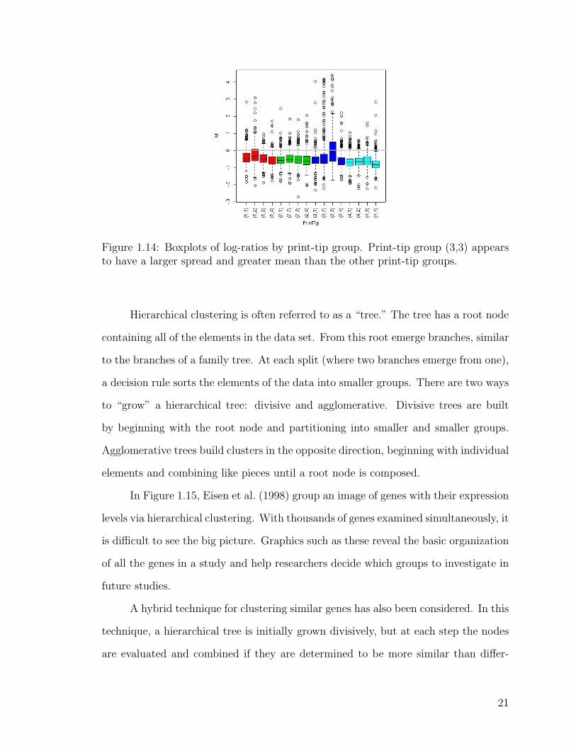
Figure 1.14: Boxplots of log-ratios by print-tip group. Print-tip group (3,3) appearsto have a larger spread and greater mean than the other print-tip groups.

Hierarchical clustering is often referred to as a “tree.” The tree has a root node

containing all of the elements in the data set. From this root emerge branches, similar

to the branches of a family tree. At each split (where two branches emerge from one),

a decision rule sorts the elements of the data into smaller groups. There are two ways

to “grow” a hierarchical tree: divisive and agglomerative. Divisive trees are built

by beginning with the root node and partitioning into smaller and smaller groups.

Agglomerative trees build clusters in the opposite direction, beginning with individual

elements and combining like pieces until a root node is composed.

In Figure 1.15, Eisen et al. (1998) group an image of genes with their expression

levels via hierarchical clustering. With thousands of genes examined simultaneously, it

is difficult to see the big picture. Graphics such as these reveal the basic organization

of all the genes in a study and help researchers decide which groups to investigate in

future studies.

A hybrid technique for clustering similar genes has also been considered. In this

technique, a hierarchical tree is initially grown divisively, but at each step the nodes

are evaluated and combined if they are determined to be more similar than differ-

21

ent. The HOPACH algorithm (van der Laan and Pollard 2003) uses this alternating

partitioning and collapsing to create a hierarchical tree. The HOPACH (Hierarchical

Ordered Partitioning and Collapsing Hybrid) algorithm to choose the number of di-

visions to create at each node, which clusters to combine, and which clusters to keep

as the main clusters. This algorithm utilizes the median split silhouette criterion

(Pollard and van der Laan 2002a), a technique for selecting the number of clusters,

to accomplish these tasks. One of the strengths of HOPACH is its ability to create a

non-binary tree; it is not limited to binary splits, but can split a parent node into as

many daughter nodes as deemed necessary.

K-means is another clustering algorithm designed to organize data without

making any distributional assumptions. The goal is to divide the data into K clusters

such that the within-cluster sum of squares is minimized. This algorithm recognizes

the impracticality of minimizing the global sums of squares in a large data set due to

the enormous amount of possible partitions; consequently, local minima are sought

and the results are deemed sufficient.

The K-means algorithm iteratively moves points from one cluster to another

until no further move will reduce the within-cluster sums of squares. The initial set

of K clusters is chosen arbitrarily such that each cluster contains at least one point and

the mean of each cluster is computed. Each point is evaluated to determine if within-

cluster sums of squares can be reduced by moving the point to a different cluster.

This process is repeated until the within-cluster sums of squares are minimized.

K-means is a simple, efficient algorithm requiring few assumptions about the

data. It does, however, have some limitations. Unlike the HOPACH algorithm, the

number of clusters must be specified prior to classifying the data. Hence, K-means

should only be used if the researcher has a priori information about the number of

clusters.

Like hierarchical clustering and K-means, self-organizing maps (SOM’s) seek to

22

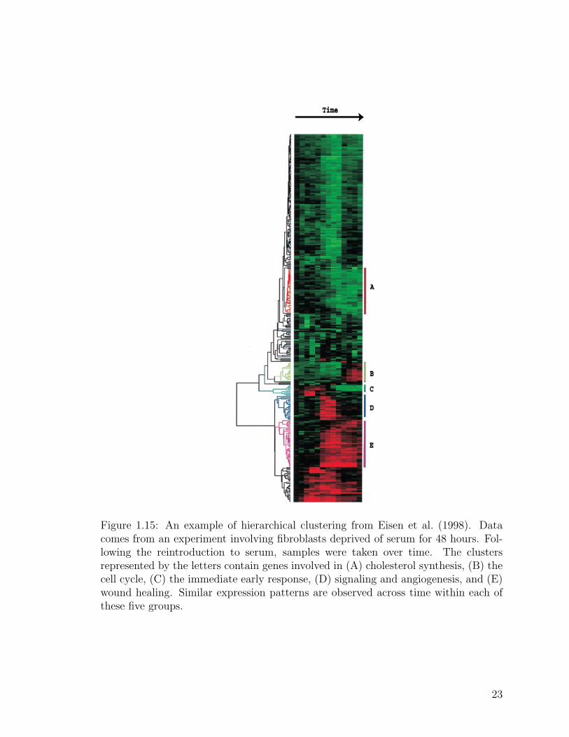
Figure 1.15: An example of hierarchical clustering from Eisen et al. (1998). Datacomes from an experiment involving fibroblasts deprived of serum for 48 hours. Fol-lowing the reintroduction to serum, samples were taken over time. The clustersrepresented by the letters contain genes involved in (A) cholesterol synthesis, (B) thecell cycle, (C) the immediate early response, (D) signaling and angiogenesis, and (E)wound healing. Similar expression patterns are observed across time within each ofthese five groups.

23

discover the underlying structure or pattern in a data set. SOM’s, however, have a

number of benefits over these other methods when clustering gene expression data.

Less structured than the rigid hierarchical clustering, but more structured than the

unassuming K-means, SOM’s have proven to be more robust than either alternative

method.

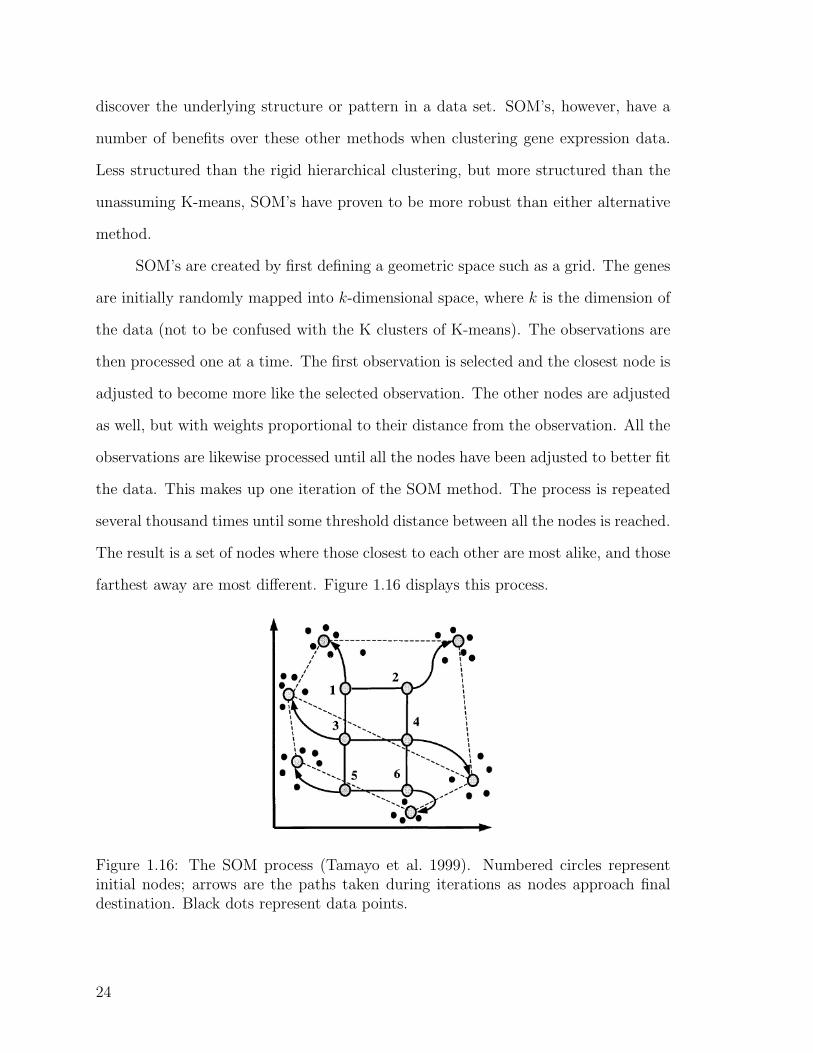
SOM’s are created by first defining a geometric space such as a grid. The genes

are initially randomly mapped into k-dimensional space, where k is the dimension of

the data (not to be confused with the K clusters of K-means). The observations are

then processed one at a time. The first observation is selected and the closest node is

adjusted to become more like the selected observation. The other nodes are adjusted

as well, but with weights proportional to their distance from the observation. All the

observations are likewise processed until all the nodes have been adjusted to better fit

the data. This makes up one iteration of the SOM method. The process is repeated

several thousand times until some threshold distance between all the nodes is reached.

The result is a set of nodes where those closest to each other are most alike, and those

farthest away are most different. Figure 1.16 displays this process.

Figure 1.16: The SOM process (Tamayo et al. 1999). Numbered circles representinitial nodes; arrows are the paths taken during iterations as nodes approach finaldestination. Black dots represent data points.

24

Akin to hierarchical clustering, gene shaving (Hastie et al. 2000) extracts subsets

of genes with related expression patterns and large variation across the conditions

being studied. Unlike hierarchical clustering, gene shaving allows genes to fall in

more than one subset. The algorithm behind gene shaving requires a predefined α

(proportion of genes to be “shaved” at each iteration) and M (the maximum number

of final clusters).

The first step of the gene shaving algorithm is to center the X matrix of gene

expression so that each row has a mean of 0. Next, compute the leading principal

component of each row. Remove, or “shave,” α of the genes with the smallest absolute

inner-product with the leading principal component. Then, continue computing prin-

ciple components and shaving genes until only one gene is left. With each iteration,

a new subset of genes is formed (SN ⊃ Sk ⊃ Sk1 ⊃ . . . ⊃ S1, where k is the number

of genes in the subset.) The optimal cluster, Sk, is estimated using a gap statistic

defined to find the most correlated cluster of genes. Each row of X is orthogonalized

to xSk, the mean expression of Sk. Finally, the entire process is repeated, finding a

new cluster with each iteration, until M clusters have been found. Like hierarchical

clustering, gene shaving can be unsupervised; however, if information known a pri-

ori about the data is useful in determining clusters, gene shaving has a supervised

counterpart.

1.2.3.3 Inference

Despite its relative newness, microarray technology has triggered a large col-

lection of literature regarding its analysis. Although the proposed methods are too

numerous to include in the scope of this thesis, a few prominent models merit some

further description.

Although the two-sample t-test is a good initial approach to microarray analysis,

it has proved problematic. Gene expression data often has very small variances re-

25

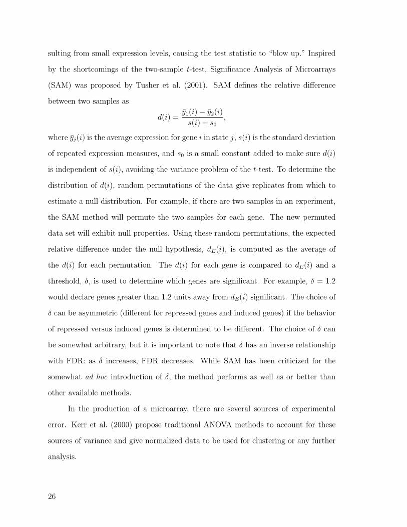
sulting from small expression levels, causing the test statistic to “blow up.” Inspired

by the shortcomings of the two-sample t-test, Significance Analysis of Microarrays

(SAM) was proposed by Tusher et al. (2001). SAM defines the relative difference

between two samples as

d(i) =y1(i)− y2(i)

s(i) + s0

,

where yj(i) is the average expression for gene i in state j, s(i) is the standard deviation

of repeated expression measures, and s0 is a small constant added to make sure d(i)

is independent of s(i), avoiding the variance problem of the t-test. To determine the

distribution of d(i), random permutations of the data give replicates from which to

estimate a null distribution. For example, if there are two samples in an experiment,

the SAM method will permute the two samples for each gene. The new permuted

data set will exhibit null properties. Using these random permutations, the expected

relative difference under the null hypothesis, dE(i), is computed as the average of

the d(i) for each permutation. The d(i) for each gene is compared to dE(i) and a

threshold, δ, is used to determine which genes are significant. For example, δ = 1.2

would declare genes greater than 1.2 units away from dE(i) significant. The choice of

δ can be asymmetric (different for repressed genes and induced genes) if the behavior

of repressed versus induced genes is determined to be different. The choice of δ can

be somewhat arbitrary, but it is important to note that δ has an inverse relationship

with FDR: as δ increases, FDR decreases. While SAM has been criticized for the

somewhat ad hoc introduction of δ, the method performs as well as or better than

other available methods.

In the production of a microarray, there are several sources of experimental

error. Kerr et al. (2000) propose traditional ANOVA methods to account for these

sources of variance and give normalized data to be used for clustering or any further

analysis.

26

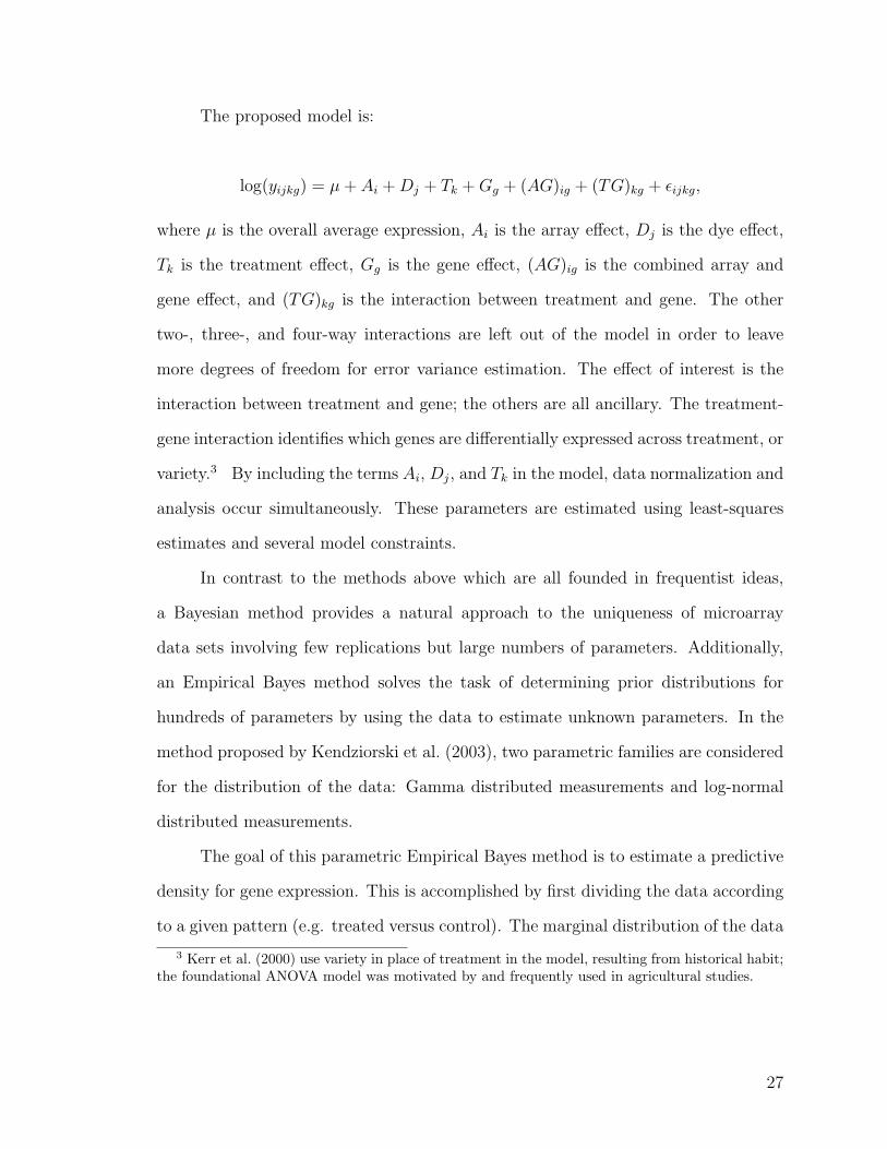
The proposed model is:

log(yijkg) = µ + Ai + Dj + Tk + Gg + (AG)ig + (TG)kg + εijkg,

where µ is the overall average expression, Ai is the array effect, Dj is the dye effect,

Tk is the treatment effect, Gg is the gene effect, (AG)ig is the combined array and

gene effect, and (TG)kg is the interaction between treatment and gene. The other

two-, three-, and four-way interactions are left out of the model in order to leave

more degrees of freedom for error variance estimation. The effect of interest is the

interaction between treatment and gene; the others are all ancillary. The treatment-

gene interaction identifies which genes are differentially expressed across treatment, or

variety.3 By including the terms Ai, Dj, and Tk in the model, data normalization and

analysis occur simultaneously. These parameters are estimated using least-squares

estimates and several model constraints.

In contrast to the methods above which are all founded in frequentist ideas,

a Bayesian method provides a natural approach to the uniqueness of microarray

data sets involving few replications but large numbers of parameters. Additionally,

an Empirical Bayes method solves the task of determining prior distributions for

hundreds of parameters by using the data to estimate unknown parameters. In the

method proposed by Kendziorski et al. (2003), two parametric families are considered

for the distribution of the data: Gamma distributed measurements and log-normal

distributed measurements.

The goal of this parametric Empirical Bayes method is to estimate a predictive

density for gene expression. This is accomplished by first dividing the data according

to a given pattern (e.g. treated versus control). The marginal distribution of the data

3 Kerr et al. (2000) use variety in place of treatment in the model, resulting from historical habit;the foundational ANOVA model was motivated by and frequently used in agricultural studies.

27

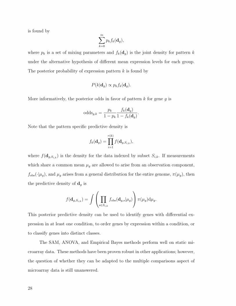
is found bym∑

k=0

pkfk(dg),

where pk is a set of mixing parameters and fk(dg) is the joint density for pattern k

under the alternative hypothesis of different mean expression levels for each group.

The posterior probability of expression pattern k is found by

P (k|dg) ∝ pkfk(dg).

More informatively, the posterior odds in favor of pattern k for gene g is

oddsg,k =pk

1− pk

fk(dg)

1− fk(dg).

Note that the pattern specific predictive density is

fk(dg) =

r(k)∏i=1

f(dg,Si,k),

where f(dg,Si,k) is the density for the data indexed by subset Si,k. If measurements

which share a common mean µg are allowed to arise from an observation component,

fobs(·|µg), and µg arises from a general distribution for the entire genome, π(µg), then

the predictive density of dg is

f(dg,Si,k) =

∫ ∏s∈Si,k

fobs(dg,s|µg)

π(µg)dµg.

This posterior predictive density can be used to identify genes with differential ex-

pression in at least one condition, to order genes by expression within a condition, or

to classify genes into distinct classes.

The SAM, ANOVA, and Empirical Bayes methods perform well on static mi-

croarray data. These methods have been proven robust in other applications; however,

the question of whether they can be adapted to the multiple comparisons aspect of

microarray data is still unanswered.

28

1.2.3.4 Multiple Comparisons

When determining significance of multiple comparisons, the family-wise error

rate—the probability of making one or more Type I errors in a group of comparisons—

is typically used in place of α. When analyzing microarray data, commonly used

controls of the family-wise error rate are generally too conservative. Benjamini

and Hochberg (1995) suggest controlling an alternative rate, the false discovery rate

(FDR), which offers some distinct advantages over traditional methods. The FDR is

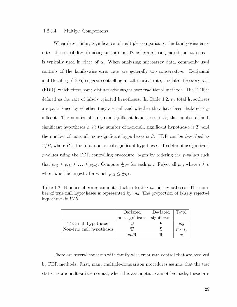
defined as the rate of falsely rejected hypotheses. In Table 1.2, m total hypotheses

are partitioned by whether they are null and whether they have been declared sig-

nificant. The number of null, non-significant hypotheses is U ; the number of null,

significant hypotheses is V ; the number of non-null, significant hypotheses is T ; and

the number of non-null, non-significant hypotheses is S. FDR can be described as

V/R, where R is the total number of significant hypotheses. To determine significant

p-values using the FDR controlling procedure, begin by ordering the p-values such

that p(1) ≤ p(2) ≤ . . . ≤ p(m). Compute im

q∗ for each p(i). Reject all p(i) where i ≤ k

where k is the largest i for which p(i) ≤ im

q∗.

Table 1.2: Number of errors committed when testing m null hypotheses. The num-ber of true null hypotheses is represented by m0. The proportion of falsely rejectedhypotheses is V/R.

Declared Declared Totalnon-significant significant

True null hypotheses U V m0

Non-true null hypotheses T S m-m0

m-R R m

There are several concerns with family-wise error rate control that are resolved

by FDR methods. First, many multiple-comparison procedures assume that the test

statistics are multivariate normal; when this assumption cannot be made, these pro-

29

cedures fall short. The FDR does not require multivariate normal test statistics and

therefore can be used no matter the test statistic’s distribution. Second, family-wise

error rate control typically has less power than single comparisons made at the same

level. Though FDR also has less power than single comparisons, it has more power

than family-wise error rate methods. Third, family-wise error rates control the prob-

ability of making at least one error. In cases of large numbers of hypotheses, this may

be too stringent of a control. For instance, when testing 1000 hypotheses, one may

be willing to accept more than one falsely rejected hypothesis. Ten falsely rejected

hypotheses are still reasonable and will allow greater power than a more stringent

cut-off. In microarray studies, there is little concern over rejecting a few true null

hypotheses. Not only does microarray data analysis involve thousands of compar-

isons, but researchers are more willing to make false discoveries since microarrays are

almost always used as a screening device.

There are some interesting comparisons between FDR and family-wise error

rate methods relating to power. FDR controlling procedures uniformly have more

power than other methods. It is important to note that all methods have a decrease

in power as the number of hypotheses increases; however, FDR methods see less of a

decrease in power than other methods.

30

2. REVIEW OF METHODS

Though a fairly recent development, microarrays are quickly becoming a widely

used tool in gene analysis. Only slightly fewer than the number of labs using microar-

rays today is the number of methods to analyze microarray data. The more specific

area of longitudinal microarray data is no different. As of yet, there is no determined

“best” method when it comes to longitudinal microarray data, but there are plenty

of ideas that claim to have good properties and valid results. Some use traditional

statistical ideas such as least squares and maximum likelihood estimates, others take

advantage of more modern approaches like empirical Bayes and hidden Markov mod-

els. A comparison of these techniques is needed to evaluate the effectiveness and

efficiency of each method.

2.1 A Modified F -statistic

Storey et al. (2005) propose a modification of existing methods, specifically

spline-based methods, to approach the time course problem. This method is applied

to two recent studies. The method developed by Storey et al. has variations to

fit two different types of time course data: comparisons within a single group and

comparisons between two or more groups. The goal of the method is to identify

patterns over time within a single group or differentially expressed genes over time

between groups. This method fits two models, one under the null hypothesis of

no differential expression over time among groups and one under the alternative

hypothesis of differential expression over time among groups. Figure 2.1 displays

these two models. The null hypothesis treats all data as one group and finds the

“best” fit over time (solid line). The alternative model divides the data into groups

(in this case, drug and placebo) and fits a model for each group (dotted lines). Each

31

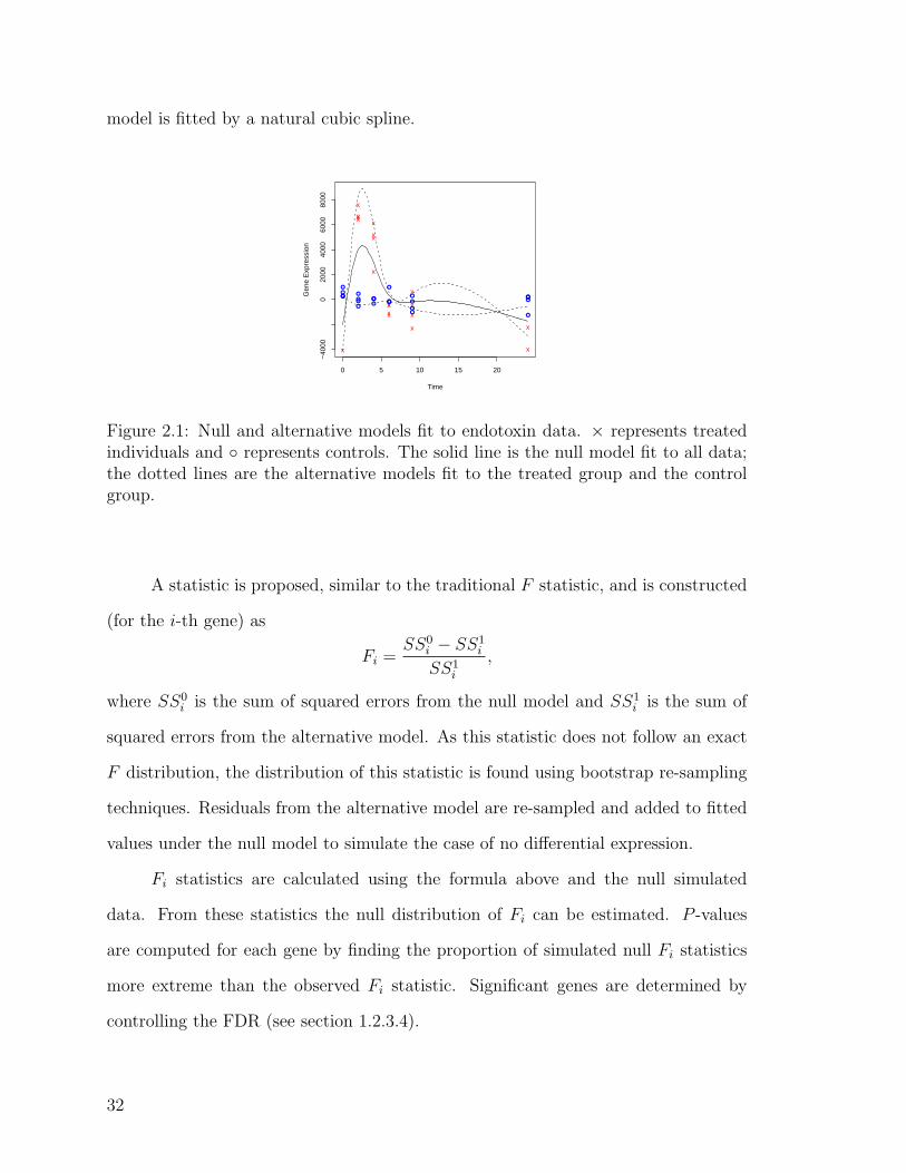
model is fitted by a natural cubic spline.

0 5 10 15 20

−40

000

2000

4000

6000

8000

Time

Gen

e E

xpre

ssio

n

xx

x

x

xxx

x

xx

x

x

xxxx

x

xx

x

x

x

x

x

●●

●

●●

●●

●

●●●

●●

●

●

●

●●

●

●●●

Figure 2.1: Null and alternative models fit to endotoxin data. × represents treatedindividuals and ◦ represents controls. The solid line is the null model fit to all data;the dotted lines are the alternative models fit to the treated group and the controlgroup.

A statistic is proposed, similar to the traditional F statistic, and is constructed

(for the i-th gene) as

Fi =SS0

i − SS1i

SS1i

,

where SS0i is the sum of squared errors from the null model and SS1

i is the sum of

squared errors from the alternative model. As this statistic does not follow an exact

F distribution, the distribution of this statistic is found using bootstrap re-sampling

techniques. Residuals from the alternative model are re-sampled and added to fitted

values under the null model to simulate the case of no differential expression.

Fi statistics are calculated using the formula above and the null simulated

data. From these statistics the null distribution of Fi can be estimated. P -values

are computed for each gene by finding the proportion of simulated null Fi statistics

more extreme than the observed Fi statistic. Significant genes are determined by

controlling the FDR (see section 1.2.3.4).

32

2.2 A Dependent Correlation Matrix

With typical longitudinal data, the key to accounting for time in the analysis

is a dependent correlation matrix. Time course data cannot be assumed to be inde-

pendent; in fact, it is almost always strongly correlated due to time dependence. At

least two authors incorporated this correlation matrix into their proposed methods.

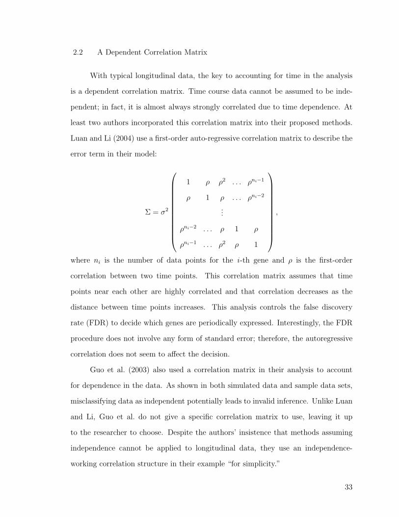
Luan and Li (2004) use a first-order auto-regressive correlation matrix to describe the

error term in their model:

Σ = σ2

1 ρ ρ2 . . . ρni−1

ρ 1 ρ . . . ρni−2

...

ρni−2 . . . ρ 1 ρ

ρni−1 . . . ρ2 ρ 1

,

where ni is the number of data points for the i -th gene and ρ is the first-order

correlation between two time points. This correlation matrix assumes that time

points near each other are highly correlated and that correlation decreases as the

distance between time points increases. This analysis controls the false discovery

rate (FDR) to decide which genes are periodically expressed. Interestingly, the FDR

procedure does not involve any form of standard error; therefore, the autoregressive

correlation does not seem to affect the decision.

Guo et al. (2003) also used a correlation matrix in their analysis to account

for dependence in the data. As shown in both simulated data and sample data sets,

misclassifying data as independent potentially leads to invalid inference. Unlike Luan

and Li, Guo et al. do not give a specific correlation matrix to use, leaving it up

to the researcher to choose. Despite the authors’ insistence that methods assuming

independence cannot be applied to longitudinal data, they use an independence-

working correlation structure in their example “for simplicity.”

33

2.3 A Robust Wald Statistic

As one of the pioneer papers in analyzing longitudinal gene expression data, the

methods used by Guo et al. approach longitudinal gene expression analysis using a

basic generalization of simple techniques. The paper proposes a robust Wald statistic

for the ith gene of the form

W (i) = [Lβ(i)]′[LVS(i)L′]−1[Lβ(i)],

where VS(i) takes a working correlation matrix into account. The statistic is consid-

ered “robust” because it uses permutation methods to create an accurate sampling

distribution of the test statistic even though the sample size is small.

Also defined in the paper is the gene-specific score,

w(i) = [Lβ(i)]′[LVSL′ + λwIr×r]−1[Lβ(i)],

which incorporates a small value in the denominator to solve singularity and normal-

ization problems.

2.4 Guide Genes

Luan and Li propose a method using “guide genes,” genes known to be peri-

odically regulated. These include genes involved in cell cycle regulation as well as

those involved in circadian rhythmic regulation—rhythms expressed over a 24-hour

time period. From these genes, a general function for all cyclically expressed genes

can be estimated. The functions of genes with unknown regulation patterns can then

be compared to this “standard” function and, using likelihood ratio tests, determined

to be of the same cyclic pattern or not.

The idea behind this model-based approach begins by estimating the model for

the guide genes using a cubic B-spline-based periodic function. The model for all

34

genes (guide and otherwise) assumes

Yij = µi + βif(tij − τi) + εij

for gene i and observation j where µi is the mean gene expression level for the ith gene,

f is the common function of the guide genes, tij is the time when the ijth sample was

taken, and βi and τi are location and scale parameters for the ith gene. The model

for the unknown genes is assumed to be computed in a similar fashion, although the

paper is not clear on this point. To determine whether the unknown genes follow the

same pattern as the guide genes, the test βi = 0 is performed. If βi = 0, the model

becomes

Yij = µi + εij.

Since this model does not include any time effect, it is equivalently testing the peri-

odicity of each gene.

2.5 Mixture Analysis

Although genes are often classified by their function, this does not necessarily

mean that functionally similar genes, or classes, follow the same expression patterns.

Gui and Li (2003) introduce a method to distinguish between mixtures of expression

patterns within a classification group. The method, mixture functional discriminant

analysis (MFDA), uses B-splines and the EM algorithm to estimate a likelihood for

each gene, then evokes maximum likelihood to determine which subclass the gene lies

in.

To demonstrate the accuracy of MFDA, three classes are simulated, two of

which are single classes and one of which is a mixture of 4 subclasses. MFDA is

compared to three other methods using this simulated data set. MFDA appears to

outperform the others (MDA, FLDA, and LDA). A real data set of yeast cells is

also analyzed using these four methods. Reserving one-third of the genes to use for

35

validation purposes, the misclassification rates are compared for the methods. In

general, MFDA again performs best.

2.6 Hidden Markov Models

Identifying differential expression over time is a daunting task with microarray

experiments. Many researchers will attempt to treat each time point as indepen-

dent of one another and use traditional approaches for determining significance, but

time course data exhibits dependence due to time which violates the independence

assumption. Yuan et al. (2003) proposed a method using Markov chains to account

for this dependence and determine the expression patterns over time in microarray

data.

The method begins by identifying patterns, or states, of interest. For example,

if there are three biological conditions, there are five possible expression states: µ1 =

µ2 = µ3 or µ1 = µ2 6= µ3 or µ1 6= µ2 = µ3 and so on. The goal is to estimate the

most probable set of states over time. To estimate the probability of each state, the

expression patterns are assumed to follow a Markov chain. That is, the probability

of a given state j at time t is πj(t) = P (st = j). The initial probability distribution

is defined as π(1) = (π1(1), . . . , πJ(1)). The transition matrices for the Markov chain

are A(t) =(ai|j(t)

), where ai|j(t) = P (st+1 = i|st = j). Also necessary to compute

the most probable set of states is the conditional distribution xt|st = i ∼ fit(xt).

The Baum-Welch algorithm is used to estimate the initial probability distribution of

states, the transition matrices, and the conditional distribution of expression level

given a specific expression pattern. These estimates are then used in the Verbiti

algorithm to determine the most probable set of expression patterns over time.

36

2.7 Method Comparison and Evaluation

One difficulty in comparing the different analysis methods available for time

course microarray experiments is that each method does not necessarily produce the

same type of results. That is, the hypotheses being tested vary among the different

methods. For example, the guide genes method proposed by Luan and Li (2004)

explains which genes have periodic expression similar to that of the guide genes. In

contrast, the method proposed by Storey et al. (2005) seeks to determine whether each

gene shows an effect over time. Additionally, the method used by Yuan et al.’s (2003)

determines the most probable set of expression patterns over time. Consequently, it

is problematic to compare all of these methods simply on the basis of their results.

Because each method is specific to certain types of data, each method must be

evaluated individually. A simulation can provide method-specific data to investigate

a method’s power and specificity. Though evaluating each of the above methods

through simulation-based approaches is beyond the scope of this paper, the method

used by Storey et al. will be used as an example and model for future methods.

37

3. STOREY METHOD

Gene expression analyses are difficult to evaluate because the true distribution

of genetic data is extremely complicated. Estimates of gene expression data are

overly simplified and skeptical at best. Consequently, many methods exist to detect

significance in gene expression data, but there is no gold standard to decide which

method detects the type of significance a researcher is interested in.

Rather than attempting to simulate a set of genes with complex dependencies

and unknown distributions, a simulation could borrow information from existing data

to generate a gene within a reasonable range following plausible patterns. The method

can then be evaluated by appending this new gene to the existing data set and

exploring the method’s sensitivity to this new gene.

Of the methods summarized in the previous chapter, the Storey method lends

itself to investigating the simulation-based approach to gene expression analyses.

Storey et al. provide well-documented code along with their method, allowing it to

be easily recreated and modified for simulation purposes. Also, this method is inno-

vative, yet traditional and relatively simple, appeasing most audiences. This method

will be discussed in more detail in the following sections.

3.1 Motivating Experiment and Objective

Two studies motivate and illustrate the method used by Storey et al. The

first study examines the mechanisms behind endotoxin response. Endotoxin contains

lipopolysaccharide, a macromolecule found in the cell membrane of certain bacteria.

In humans, small amounts of endotoxins cause rapid physiological changes, partic-

ularly a temperature increase. Endotoxins are useful in immune response studies

because of their non-toxic nature; although endotoxins illicit an immediate immune

38

response, they do not harm their host. The endotoxin study involved eight subjects.

Each was given either endotoxin or a placebo (four in each group). At six time points,

one before treatment and five after treatment, blood was collected from each subject.

The time points after treatment were 2, 4, 6, 9, and 24 hours following treatment.

The second study differs from the first in that the observations are independent.

Human subjects ranging from 24 to 92 years old were used to study the effect of age

on the kidneys. Kidney tissue was extracted from each subject for the study. The goal

of this investigation was to determine which, if any, genes show differential expression

over time in kidney tissue. Because following a group of subjects over 50 years is

impractical in this case, the independent sampling scheme used here is appropriate.

Both motivating studies examine differential gene expression over time. In

the first study, a static experiment would partially reveal which genes are affected

by endotoxin, but would fail in identifying genes affected at different stages following

endotoxin introduction. A time course experiment is necessary to identify which genes

show differential expression. In the kidney study, one may be tempted to treat the

data as static because the observations are independent; however, current methods

for static data are designed for unordered categorical conditions. Time is neither

unordered nor categorical; thus, a time course method is necessary for the kidney

data as well. This design also proves advantageous when the data is not balanced or

only one observation is available for each time point. Whereas a method for static

data requires imputing missing data or arbitrary measures to compensate for these

conditions, this method borrows information inherent in the time variable to avoid

unnecessary assumptions.

3.2 Detecting Differential Gene Expression

The method developed by Storey et al. has variations to fit two different types

of time course data: comparisons within a single group and comparisons between two

39

or more groups. For the purpose of this thesis, the method will be described as it

applies to the endotoxin data, which is a comparison between two groups. The goal of

the endotoxin study is to identify differentially expressed genes over time between the

endotoxin group and the placebo group. That is, the investigators want to identify

which genes show significantly different patterns over time when exposed to endotoxin

versus unexposed to endotoxin.

This method fits two models, one under the null hypothesis of no differential

expression over time among the groups and one under the alternative hypothesis of

differential expression over time among the groups. Figure 2.1 displays these two

models. The null hypothesis treats all data as one group and finds the “best” fit over

time (solid line). The alternative model divides the data by endotoxin-treated and

placebo and fits a model for each group (dotted lines). These models are fitted using

a natural cubic spline.1

A statistic is proposed, similar to the traditional F statistic, and is constructed

(for the i-th gene) as

Fi =SS0

i − SS1i

SS1i

,

where SS0i is the sum of squared errors from the null model and SS1

i is the sum of

squared errors from the alternative model. In a traditional F statistic, the random

errors are assumed to follow a Normal deviation. The random errors in the above

statistic do not follow this assumption; therefore, the statistic does not follow an exact

F distribution. The distribution of this statistic is found using bootstrap re-sampling

techniques. Residuals from the alternative model are re-sampled and added to fitted

values under the null model to simulate the case of no differential expression. The

sampled residuals come from the alternative model because the alternative model

makes no assumptions concerning whether the null or alternative hypotheses are

true. These residuals are added to the null model fit because the class of null models

1 Another option is to use a polynomial basis, which proved effective in both studies, but is lessflexible and more assumptive than the natural cubic spline (Storey et al. 2005).

40

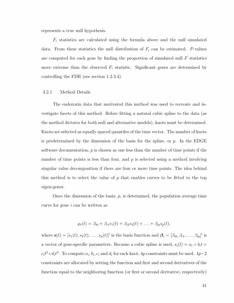
represents a true null hypothesis.

Fi statistics are calculated using the formula above and the null simulated

data. From these statistics the null distribution of Fi can be estimated. P -values

are computed for each gene by finding the proportion of simulated null F statistics

more extreme than the observed Fi statistic. Significant genes are determined by

controlling the FDR (see section 1.2.3.4).

3.2.1 Method Details

The endotoxin data that motivated this method was used to recreate and in-

vestigate facets of this method. Before fitting a natural cubic spline to the data (as

the method dictates for both null and alternative models), knots must be determined.

Knots are selected as equally spaced quantiles of the time vector. The number of knots

is predetermined by the dimension of the basis for the spline, or p. In the EDGE

software documentation, p is chosen as one less than the number of time points if the

number of time points is less than four, and p is selected using a method involving

singular value decomposition if there are four or more time points. The idea behind

this method is to select the value of p that enables curves to be fitted to the top

eigen-genes.

Once the dimension of the basis, p, is determined, the population average time

curve for gene i can be written as

µt(t) = βi0 + βi1s1(t) + βi2s2(t) + . . . + βipsp(t),

where s(t) = [s1(t), s2(t), . . . , sp(t)]′ is the basis function and βi = [βi0, βi1, . . . , βip]

′ is

a vector of gene-specific parameters. Because a cubic spline is used, si(t) = ai + bit +

cit2+dit

3. To compute ai, bi, ci and di for each knot, 4p constraints must be used. 4p−2

constraints are allocated by setting the function and first and second derivatives of the

function equal to the neighboring function (or first or second derivative, respectively)

41

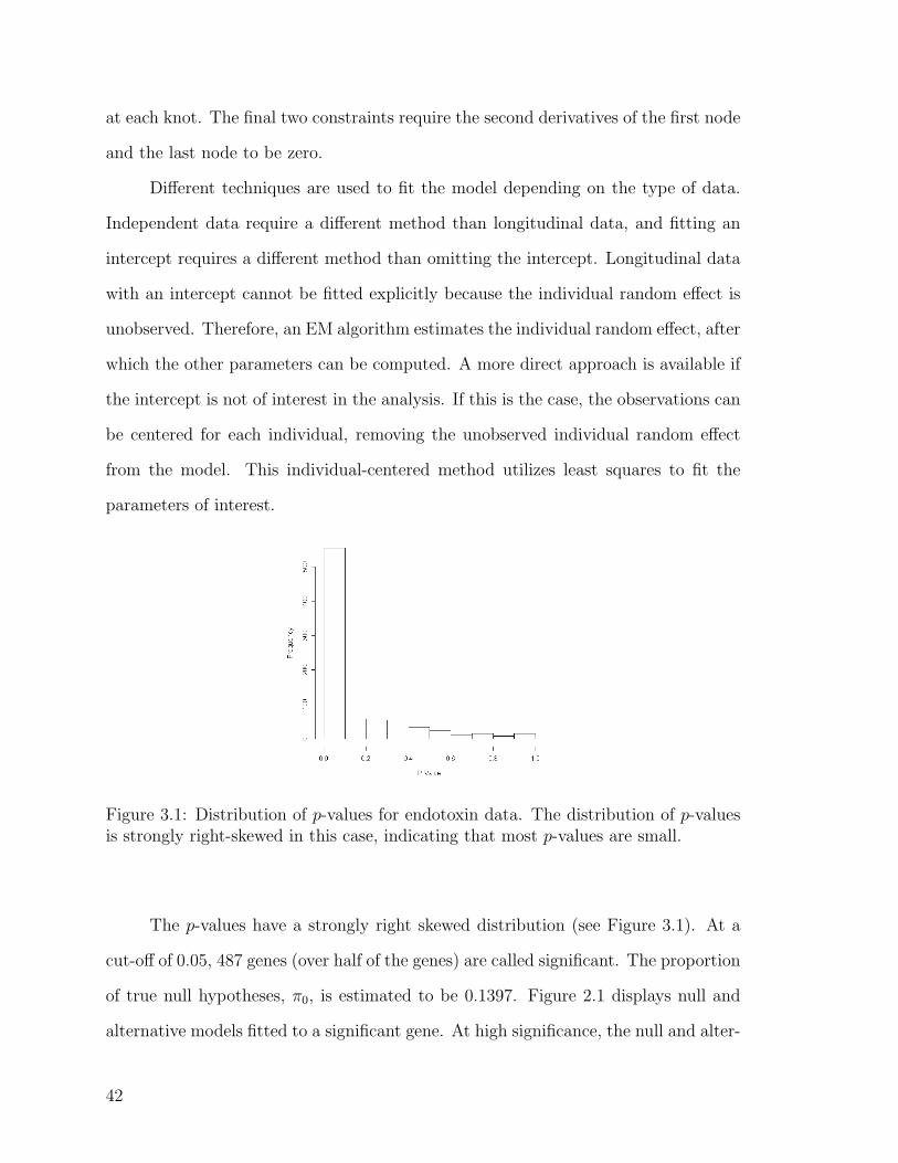
at each knot. The final two constraints require the second derivatives of the first node

and the last node to be zero.

Different techniques are used to fit the model depending on the type of data.

Independent data require a different method than longitudinal data, and fitting an

intercept requires a different method than omitting the intercept. Longitudinal data

with an intercept cannot be fitted explicitly because the individual random effect is

unobserved. Therefore, an EM algorithm estimates the individual random effect, after

which the other parameters can be computed. A more direct approach is available if

the intercept is not of interest in the analysis. If this is the case, the observations can

be centered for each individual, removing the unobserved individual random effect

from the model. This individual-centered method utilizes least squares to fit the

parameters of interest.

Figure 3.1: Distribution of p-values for endotoxin data. The distribution of p-valuesis strongly right-skewed in this case, indicating that most p-values are small.

The p-values have a strongly right skewed distribution (see Figure 3.1). At a

cut-off of 0.05, 487 genes (over half of the genes) are called significant. The proportion

of true null hypotheses, π0, is estimated to be 0.1397. Figure 2.1 displays null and

alternative models fitted to a significant gene. At high significance, the null and alter-

42

native models are obviously distinct and significance is apparent. At non-significance,

the models overlap, often indicating that the null model is just as appropriate for the

gene as the alternative models. At either extreme, a graphical display of the data and

the models fitted to the data is enough to determine significance. When a gene falls in

the middle (neither highly significant nor highly non-significant), a more quantitative

cut-off is necessary.

The R code for all implementation is included in Appendix A. The func-

tions get.pvalues and mat.sq are borrowed from the EDGE software developed

by Alan Dabney, Jeffrey Leek, Eva Monsen, and John Storey. The remainder of the

storey.sim function is modeled after components of the EDGE software. The other

functions are original work of the author.

43

4. SIMULATION STUDY

A simple, computationally inexpensive simulation can often provide validation

of a method much more easily and quickly than a mathematical proof. Simula-

tions can also offer interesting insights into particular aspects of an analysis method.

Though typically less general than a proof, the specificity of simulations can some-

times be an advantage. This simulation validates the Storey method by simulating

data based on the features and patterns found in the endotoxin data, thus providing

a researcher using the Storey method on the endotoxin data with very detailed infor-

mation regarding which types of genes will be identified as significant. If the type of

pattern the researcher hopes to identify is not picked up by this method, this simu-

lation will identify this shortcoming before time and resources are spent on further

investigation. These simulation results can only be directly applied to this particular

combination of method and data; however, this simulation approach can be applied

to any study.

The first task of any simulation is deciding how to generate data. Once the

specifics for simulating data are established, features of the data can be manipulated

to study the method. Finally, the results reveal important aspects of the method’s

limits of detection. Each of these steps are performed on the endotoxin data from

Storey et al.

4.1 Simulating Gene Expression Data

Simulating gene expression data is not trivial. Biological systems are known to

be complex and individual genes are far from independent. Thus, the first task in

a gene expression simulation study is simulating feasible data. Although potentially

oversimplified, simulated gene expression data allows manipulation of characteristics

44

of the data in order to verify a method’s power.

To imitate the endotoxin data, one could simulate separate null and alternative

data to correspond to control and treated arrays, respectively. The null data would

have a constant effect over time whereas the alternative data would have a variety

of effects over time. For instance, one alternative gene could have a very defined

deviance from the null levels while another alternative gene could be just slightly

shifted from the null pattern. A third alternative gene could have the same overall

level as the null genes, but a different effect over time. The possibilities are endless,

but they may not all be reasonable. It may not be realistic to see such a combination

of patterns in a single data set. The more genetic variation induced on a simulated

data set, the more uncertainty generated as to whether the data set is plausible.

An alternative to generating an entire set of gene expression data is to manipu-

late an existing data set. For instance, the endotoxin data could be centered such that

the error introduced by each individual is subtracted out. Then, random error could

be added back to the centered data to create a new, “random” data set incorporating

all the complicated dependencies in real gene expression data. This idea is similar

to the method described in Chapter 3 used to estimate the null distribution of the

F -statistic.

A third option is to leave the existing data exactly as it is and add a single

simulated gene to the current data set. This approach is similar to the spike-in

approach, originally developed to validate expression level measurements on an array.

Spike-in genes are genes which are added to but not naturally found in the sample.

For example, arabidopsis (a flowering plant) genes may be “spiked-in” to a sample of

rat RNA. The spiked transcripts are added in known quantities, providing a standard

to compare to the other spots on the array. Similarly, adding a single simulated gene

with known features to an existing data set allows a comparison of the significance

of other genes to this known gene. This would allow investigation of the method’s

45

sensitivity and power by manipulating the single gene to exhibit various properties

(significant, nonsignificant, linear time effect, sinusoidal time effect, magnitude of

differential expression, etc.).

The third option is the approach chosen to perform this simulation study; it is

straightforward, simplistic and makes the fewest alterations to the existing data. For

purposes of this study, the expression levels for gene i and individual j are assumed

to follow a normal distribution with mean µ and have a spatial power correlation

structure, as follows:

yij = N(µj,Σ),

Σ = σ2

1 ρ2 ρ4 ρ6 ρ9 ρ24

ρ2 1 ρ2 ρ4 ρ7 ρ22

ρ4 ρ2 1 ρ2 ρ5 ρ20

ρ6 ρ4 ρ2 1 ρ3 ρ18

ρ9 ρ7 ρ5 ρ3 1 ρ15

ρ24 ρ22 ρ20 ρ18 ρ15 1

.

The covariance between time ti and tj is equal to ρ raised to the distance (in hours)

between the two time points.

Each gene has 46 observations—eight individuals each with samples taken at

six time points, except for one individual who only has samples taken at four time

points. To obtain the 46 expression values for a simulated gene, each individual’s six

(or four) time points will be computed separately using the distribution above, then

concatenated to form a 1× 46 vector to be appended to the existing data set, which

currently has dimensions of 800× 46.

The mean vector used to simulate each individual’s six (or four) time points

depends on whether the individual is from the control group or the treated group. If

the individual is from the control group, µ will be estimated using only the control

46

arrays from the original data set. If the individual is from the treated group, µ will

be estimated using only the treated arrays from the original data set. The methods

used to estimate these µ values will be discussed in Section 4.2.1.

To estimate ρ, the correlation matrix for each gene was computed. (Individual

six is missing two time points and therefore was not included in this estimation.)

For computational purposes, only the correlation matrices with no negative elements

were included.1 By excluding correlation matrices with negative elements, 375 genes

of the total 800 genes were used to estimate ρ. Each of these 375 matrices were

passed through a function that raised each element to the inverse power as exhibited

in the correlation structure above. For instance, the second element of the first row

of each estimated correlation matrix was raised to the 12

power. The average of these

transformed off-diagonal elements was retained as the ρ estimate for that gene. These

375 estimates of ρ have a slightly left-skewed distribution (see Figure 4.1); however,

the mean and median are very close (mean = 0.692, median = 0.704), so either could

be used with similar results. The median was chosen for use in this simulation.

To estimate the variance (σ2) to be used to simulate a new gene, the variance

at each time point for each gene was computed. This distribution is strongly right-

skewed (see Figure 4.2); therefore, the median will be used instead of the mean. The

median of this distribution is 262,275 squared expression units.

4.2 Varying Features of the Data

Four features of the data are evaluated in this simulation: µ, ρ, σ2, and the

magnitude of difference between control and treated array vectors. For each selected

combination of these four parameters, 1000 simulations were conducted. That is,

1 The presence of negative elements in the sample correlation matrices raises concern about thechosen correlation structure, but only 13% of the off-diagonal elements of the sample correlationmatrices were less than 0, and the median of these negative elements is -0.23. Therefore, for thepurposes of this study, the negative correlation will be assumed to be due to random noise and onlypositive values of ρ will be considered.

47

ρρ

Fre

quen

cy

0.2 0.4 0.6 0.8 1.00

2040

60

Figure 4.1: A histogram of estimates of ρ. The distribution is slightly left-skewed,but the mean and the median are close in value.

1000 new genes were simulated and concatenated one at a time to the existing 800

genes. The Storey method was used to assign each gene a p-value and q-value. As

discussed earlier, p-values are too conservative for microarray analyses; q-values are

designed such that the cut-off is chosen after the simulation is conducted, making

them an inconsistent evaluator for multiple simulations. The measurement chosen to

evaluate and compare each simulation was the number of times the new gene was

ranked in the top 100 out of all 801 genes. This is the value reported in the following

figures.

4.2.1 Choice of µ

The choice of mean vector to use as the basis for simulating a new gene can

greatly affect the results. There are many ways to estimate a reasonable mean vector

for these two groups. Three methods for choosing µ are used in this simulation.

The first method can be used to simulate null genes. These are genes that have

no statistically significant difference between treated arrays and control arrays. To

ensure these genes are truly null, both the control and treated individuals will come

from the same mean vector. This method uses all 800 genes, but only the control

48

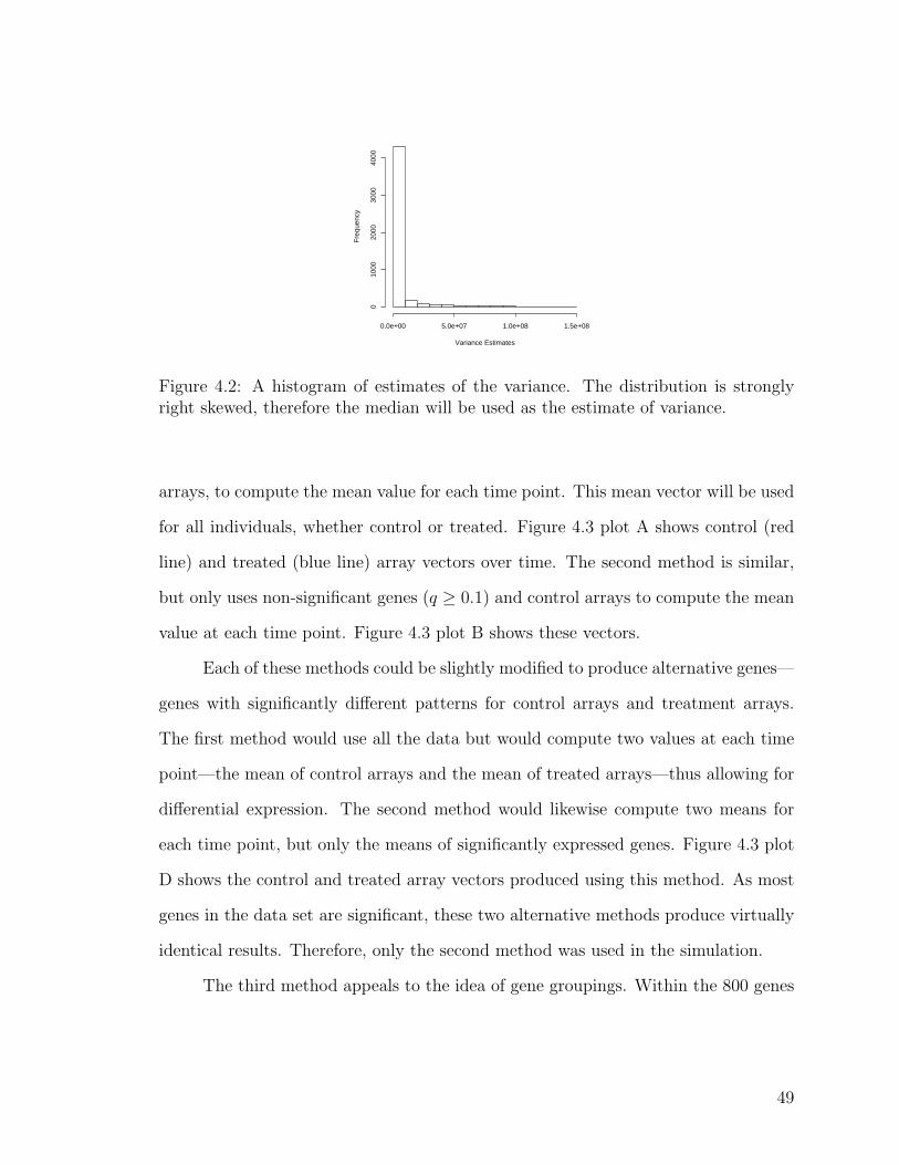
Variance Estimates

Fre

quen

cy

0.0e+00 5.0e+07 1.0e+08 1.5e+08

010

0020

0030

0040

00

Figure 4.2: A histogram of estimates of the variance. The distribution is stronglyright skewed, therefore the median will be used as the estimate of variance.

arrays, to compute the mean value for each time point. This mean vector will be used

for all individuals, whether control or treated. Figure 4.3 plot A shows control (red

line) and treated (blue line) array vectors over time. The second method is similar,

but only uses non-significant genes (q ≥ 0.1) and control arrays to compute the mean

value at each time point. Figure 4.3 plot B shows these vectors.

Each of these methods could be slightly modified to produce alternative genes—

genes with significantly different patterns for control arrays and treatment arrays.

The first method would use all the data but would compute two values at each time

point—the mean of control arrays and the mean of treated arrays—thus allowing for

differential expression. The second method would likewise compute two means for

each time point, but only the means of significantly expressed genes. Figure 4.3 plot

D shows the control and treated array vectors produced using this method. As most

genes in the data set are significant, these two alternative methods produce virtually

identical results. Therefore, only the second method was used in the simulation.

The third method appeals to the idea of gene groupings. Within the 800 genes

49

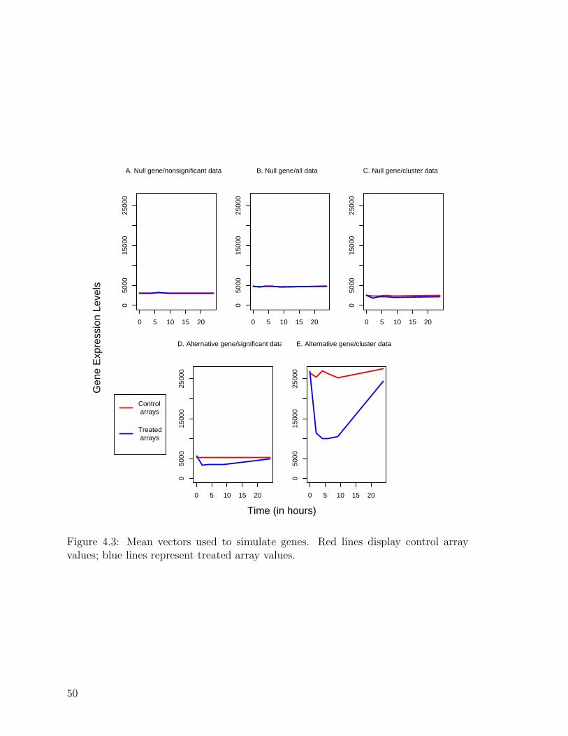
0 5 10 15 20

050

0015

000

2500

0

0 5 10 15 20

050

0015

000

2500

0

0 5 10 15 20

050

0015

000

2500

0

0 5 10 15 20

050

0015

000

2500

0

0 5 10 15 20

050

0015

000

2500

0

Gen

e E

xpre

ssio

n Le

vels

Time (in hours)

Control arrays

Treated arrays

A. Null gene/nonsignificant data B. Null gene/all data C. Null gene/cluster data

D. Alternative gene/significant data E. Alternative gene/cluster data

Figure 4.3: Mean vectors used to simulate genes. Red lines display control arrayvalues; blue lines represent treated array values.

50

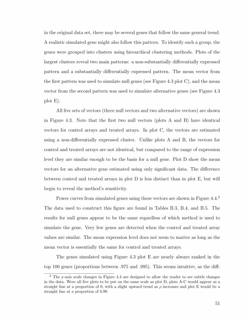
in the original data set, there may be several genes that follow the same general trend.

A realistic simulated gene might also follow this pattern. To identify such a group, the

genes were grouped into clusters using hierarchical clustering methods. Plots of the

largest clusters reveal two main patterns: a non-substantially differentially expressed

pattern and a substantially differentially expressed pattern. The mean vector from

the first pattern was used to simulate null genes (see Figure 4.3 plot C), and the mean

vector from the second pattern was used to simulate alternative genes (see Figure 4.3

plot E).

All five sets of vectors (three null vectors and two alternative vectors) are shown

in Figure 4.3. Note that the first two null vectors (plots A and B) have identical

vectors for control arrays and treated arrays. In plot C, the vectors are estimated

using a non-differentially expressed cluster. Unlike plots A and B, the vectors for

control and treated arrays are not identical, but compared to the range of expression

level they are similar enough to be the basis for a null gene. Plot D show the mean

vectors for an alternative gene estimated using only significant data. The difference

between control and treated arrays in plot D is less distinct than in plot E, but will

begin to reveal the method’s sensitivity.

Power curves from simulated genes using these vectors are shown in Figure 4.4.2

The data used to construct this figure are found in Tables B.3, B.4, and B.5. The

results for null genes appear to be the same regardless of which method is used to

simulate the gene. Very few genes are detected when the control and treated array

values are similar. The mean expression level does not seem to matter as long as the

mean vector is essentially the same for control and treated arrays.

The genes simulated using Figure 4.3 plot E are nearly always ranked in the

top 100 genes (proportions between .975 and .995). This seems intuitive, as the diff-

2 The y-axis scale changes in Figure 4.4 are designed to allow the reader to see subtle changesin the data. Were all five plots to be put on the same scale as plot D, plots A-C would appear as astraight line at a proportion of 0, with a slight upward trend as ρ increases and plot E would be astraight line at a proportion of 0.99.

51

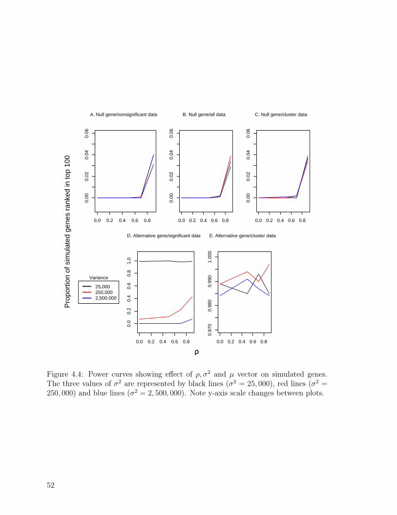
0.0 0.2 0.4 0.6 0.8

0.00

0.02

0.04

0.06

0.0 0.2 0.4 0.6 0.8

0.00

0.02

0.04

0.06

0.0 0.2 0.4 0.6 0.8

0.00

0.02

0.04

0.06

0.0 0.2 0.4 0.6 0.8

0.0

0.2

0.4

0.6

0.8

1.0

0.0 0.2 0.4 0.6 0.8

0.97

00.

980

0.99

01.

000

Pro

port

ion

of s

imul

ated

gen

es r

anke

d in

top

100

ρρ

25,000250,0002,500,000

Variance

A. Null gene/nonsignificant data B. Null gene/all data C. Null gene/cluster data

D. Alternative gene/significant data E. Alternative gene/cluster data

Figure 4.4: Power curves showing effect of ρ, σ2 and µ vector on simulated genes.The three values of σ2 are represented by black lines (σ2 = 25, 000), red lines (σ2 =250, 000) and blue lines (σ2 = 2, 500, 000). Note y-axis scale changes between plots.

52

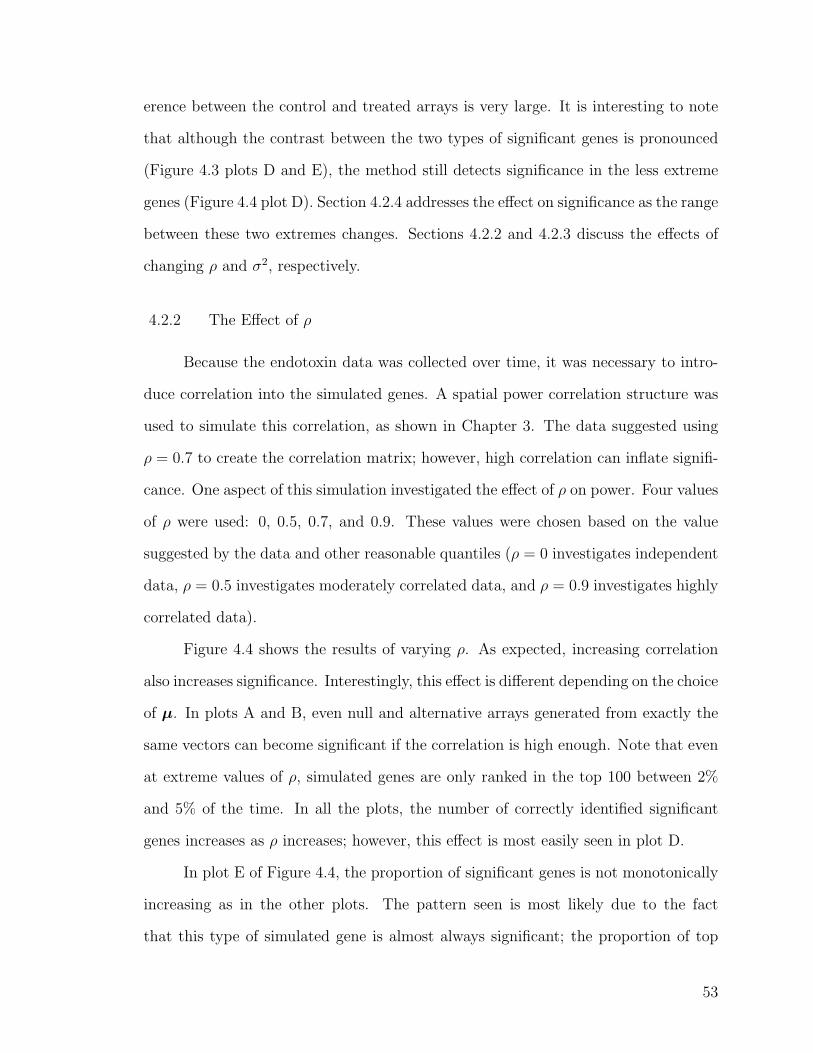
erence between the control and treated arrays is very large. It is interesting to note

that although the contrast between the two types of significant genes is pronounced

(Figure 4.3 plots D and E), the method still detects significance in the less extreme

genes (Figure 4.4 plot D). Section 4.2.4 addresses the effect on significance as the range

between these two extremes changes. Sections 4.2.2 and 4.2.3 discuss the effects of

changing ρ and σ2, respectively.

4.2.2 The Effect of ρ

Because the endotoxin data was collected over time, it was necessary to intro-

duce correlation into the simulated genes. A spatial power correlation structure was

used to simulate this correlation, as shown in Chapter 3. The data suggested using

ρ = 0.7 to create the correlation matrix; however, high correlation can inflate signifi-

cance. One aspect of this simulation investigated the effect of ρ on power. Four values

of ρ were used: 0, 0.5, 0.7, and 0.9. These values were chosen based on the value

suggested by the data and other reasonable quantiles (ρ = 0 investigates independent

data, ρ = 0.5 investigates moderately correlated data, and ρ = 0.9 investigates highly

correlated data).

Figure 4.4 shows the results of varying ρ. As expected, increasing correlation

also increases significance. Interestingly, this effect is different depending on the choice

of µ. In plots A and B, even null and alternative arrays generated from exactly the

same vectors can become significant if the correlation is high enough. Note that even

at extreme values of ρ, simulated genes are only ranked in the top 100 between 2%

and 5% of the time. In all the plots, the number of correctly identified significant

genes increases as ρ increases; however, this effect is most easily seen in plot D.

In plot E of Figure 4.4, the proportion of significant genes is not monotonically

increasing as in the other plots. The pattern seen is most likely due to the fact

that this type of simulated gene is almost always significant; the proportion of top

53

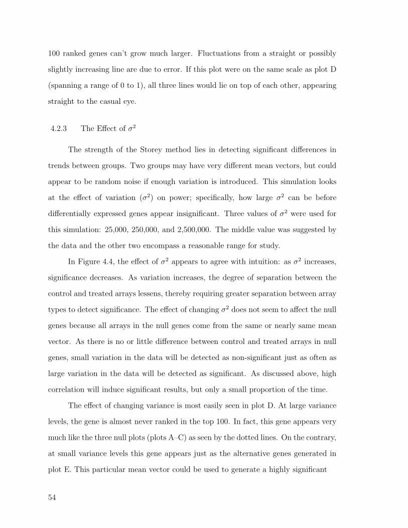
100 ranked genes can’t grow much larger. Fluctuations from a straight or possibly

slightly increasing line are due to error. If this plot were on the same scale as plot D

(spanning a range of 0 to 1), all three lines would lie on top of each other, appearing

straight to the casual eye.

4.2.3 The Effect of σ2

The strength of the Storey method lies in detecting significant differences in

trends between groups. Two groups may have very different mean vectors, but could

appear to be random noise if enough variation is introduced. This simulation looks

at the effect of variation (σ2) on power; specifically, how large σ2 can be before

differentially expressed genes appear insignificant. Three values of σ2 were used for

this simulation: 25,000, 250,000, and 2,500,000. The middle value was suggested by

the data and the other two encompass a reasonable range for study.

In Figure 4.4, the effect of σ2 appears to agree with intuition: as σ2 increases,

significance decreases. As variation increases, the degree of separation between the

control and treated arrays lessens, thereby requiring greater separation between array

types to detect significance. The effect of changing σ2 does not seem to affect the null

genes because all arrays in the null genes come from the same or nearly same mean

vector. As there is no or little difference between control and treated arrays in null

genes, small variation in the data will be detected as non-significant just as often as

large variation in the data will be detected as significant. As discussed above, high

correlation will induce significant results, but only a small proportion of the time.

The effect of changing variance is most easily seen in plot D. At large variance

levels, the gene is almost never ranked in the top 100. In fact, this gene appears very

much like the three null plots (plots A–C) as seen by the dotted lines. On the contrary,

at small variance levels this gene appears just as the alternative genes generated in

plot E. This particular mean vector could be used to generate a highly significant

54

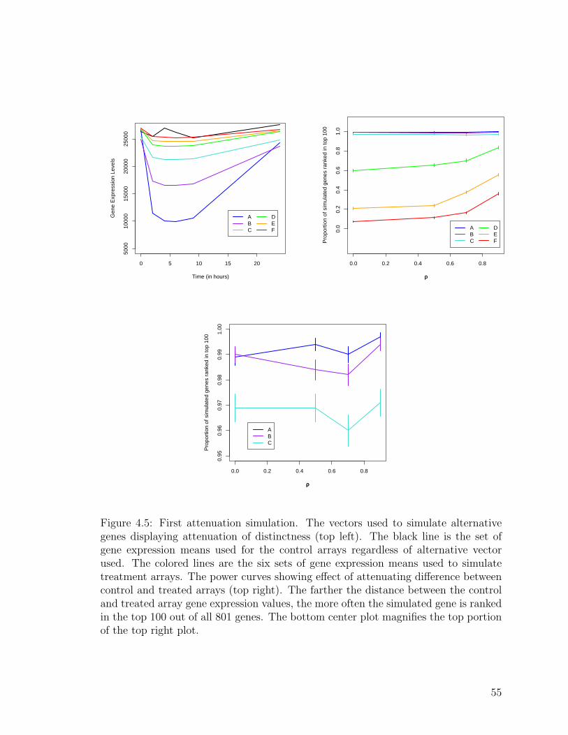
0 5 10 15 20

5000

1000

015

000

2000

025

000

Time (in hours)

Gen

e E

xpre

ssio

n Le

vels

ABC

DEF

0.0 0.2 0.4 0.6 0.8

0.0

0.2

0.4

0.6

0.8

1.0

ρρ

Pro

port

ion

of s

imul

ated

gen

es r

anke

d in

top

100

ABC

DEF

0.0 0.2 0.4 0.6 0.8

0.95

0.96

0.97

0.98

0.99

1.00

ρρ

Pro

port

ion

of s

imul

ated

gen

es r

anke

d in

top

100

ABC

Figure 4.5: First attenuation simulation. The vectors used to simulate alternativegenes displaying attenuation of distinctness (top left). The black line is the set ofgene expression means used for the control arrays regardless of alternative vectorused. The colored lines are the six sets of gene expression means used to simulatetreatment arrays. The power curves showing effect of attenuating difference betweencontrol and treated arrays (top right). The farther the distance between the controland treated array gene expression values, the more often the simulated gene is rankedin the top 100 out of all 801 genes. The bottom center plot magnifies the top portionof the top right plot.

55

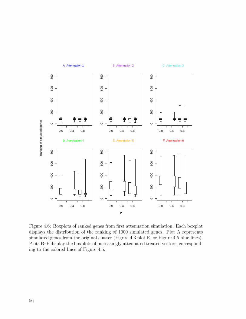
0.0 0.4 0.8

020

040

060

080

0

0.0 0.4 0.8

020

040

060

080

0

0.0 0.4 0.8

020

040

060

080

0

0.0 0.4 0.8

020

040

060

080

0

0.0 0.4 0.8

020

040

060

080

0

0.0 0.4 0.8

020

040

060

080

0

Ran

king

of s

imul

ated

gen

es

ρρ

A. Attenuation 1 B. Attenuation 2 C. Attenuation 3

D. Attenuation 4 E. Attenuation 5 F. Attenuation 6

Figure 4.6: Boxplots of ranked genes from first attenuation simulation. Each boxplotdisplays the distribution of the ranking of 1000 simulated genes. Plot A representssimulated genes from the original cluster (Figure 4.3 plot E, or Figure 4.5 blue lines).Plots B–F display the boxplots of increasingly attenuated treated vectors, correspond-ing to the colored lines of Figure 4.5.

56

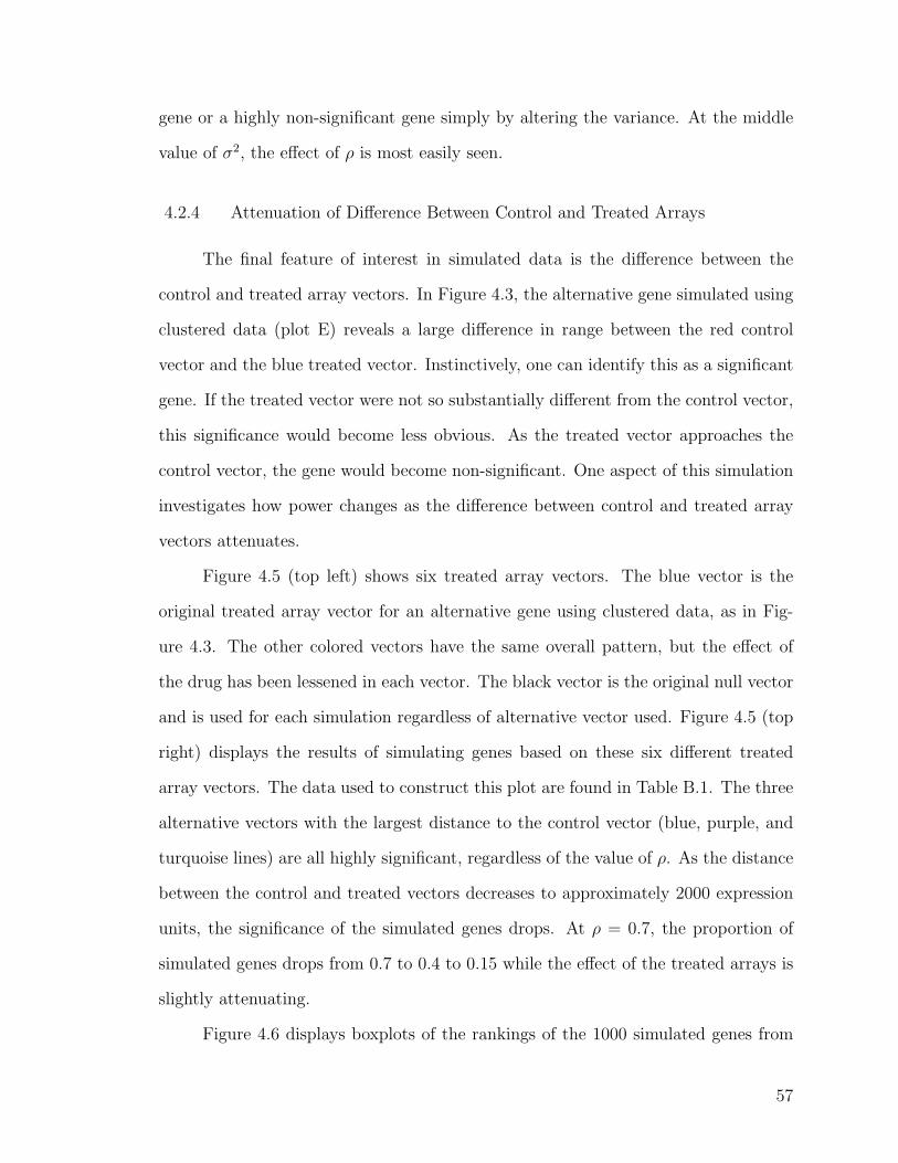
gene or a highly non-significant gene simply by altering the variance. At the middle

value of σ2, the effect of ρ is most easily seen.

4.2.4 Attenuation of Difference Between Control and Treated Arrays

The final feature of interest in simulated data is the difference between the

control and treated array vectors. In Figure 4.3, the alternative gene simulated using

clustered data (plot E) reveals a large difference in range between the red control

vector and the blue treated vector. Instinctively, one can identify this as a significant

gene. If the treated vector were not so substantially different from the control vector,

this significance would become less obvious. As the treated vector approaches the

control vector, the gene would become non-significant. One aspect of this simulation

investigates how power changes as the difference between control and treated array

vectors attenuates.

Figure 4.5 (top left) shows six treated array vectors. The blue vector is the

original treated array vector for an alternative gene using clustered data, as in Fig-

ure 4.3. The other colored vectors have the same overall pattern, but the effect of

the drug has been lessened in each vector. The black vector is the original null vector

and is used for each simulation regardless of alternative vector used. Figure 4.5 (top

right) displays the results of simulating genes based on these six different treated

array vectors. The data used to construct this plot are found in Table B.1. The three

alternative vectors with the largest distance to the control vector (blue, purple, and

turquoise lines) are all highly significant, regardless of the value of ρ. As the distance

between the control and treated vectors decreases to approximately 2000 expression

units, the significance of the simulated genes drops. At ρ = 0.7, the proportion of

simulated genes drops from 0.7 to 0.4 to 0.15 while the effect of the treated arrays is

slightly attenuating.

Figure 4.6 displays boxplots of the rankings of the 1000 simulated genes from

57

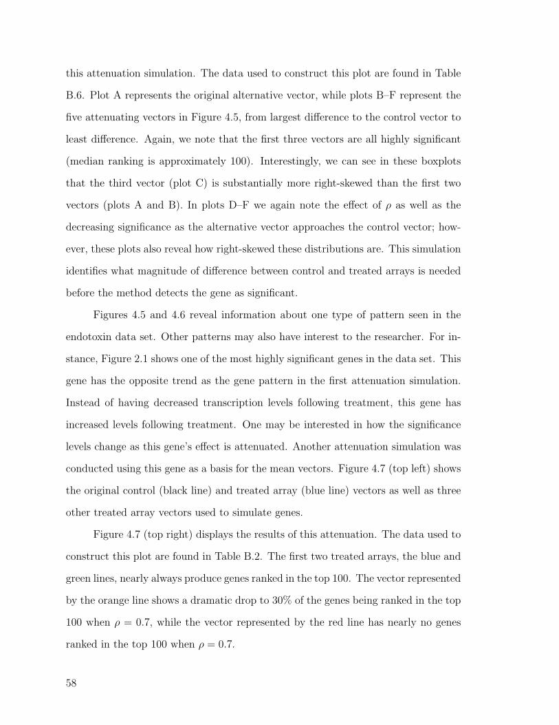
this attenuation simulation. The data used to construct this plot are found in Table

B.6. Plot A represents the original alternative vector, while plots B–F represent the

five attenuating vectors in Figure 4.5, from largest difference to the control vector to

least difference. Again, we note that the first three vectors are all highly significant

(median ranking is approximately 100). Interestingly, we can see in these boxplots

that the third vector (plot C) is substantially more right-skewed than the first two

vectors (plots A and B). In plots D–F we again note the effect of ρ as well as the

decreasing significance as the alternative vector approaches the control vector; how-

ever, these plots also reveal how right-skewed these distributions are. This simulation

identifies what magnitude of difference between control and treated arrays is needed

before the method detects the gene as significant.

Figures 4.5 and 4.6 reveal information about one type of pattern seen in the

endotoxin data set. Other patterns may also have interest to the researcher. For in-

stance, Figure 2.1 shows one of the most highly significant genes in the data set. This

gene has the opposite trend as the gene pattern in the first attenuation simulation.

Instead of having decreased transcription levels following treatment, this gene has

increased levels following treatment. One may be interested in how the significance

levels change as this gene’s effect is attenuated. Another attenuation simulation was

conducted using this gene as a basis for the mean vectors. Figure 4.7 (top left) shows

the original control (black line) and treated array (blue line) vectors as well as three

other treated array vectors used to simulate genes.

Figure 4.7 (top right) displays the results of this attenuation. The data used to

construct this plot are found in Table B.2. The first two treated arrays, the blue and

green lines, nearly always produce genes ranked in the top 100. The vector represented

by the orange line shows a dramatic drop to 30% of the genes being ranked in the top

100 when ρ = 0.7, while the vector represented by the red line has nearly no genes

ranked in the top 100 when ρ = 0.7.

58

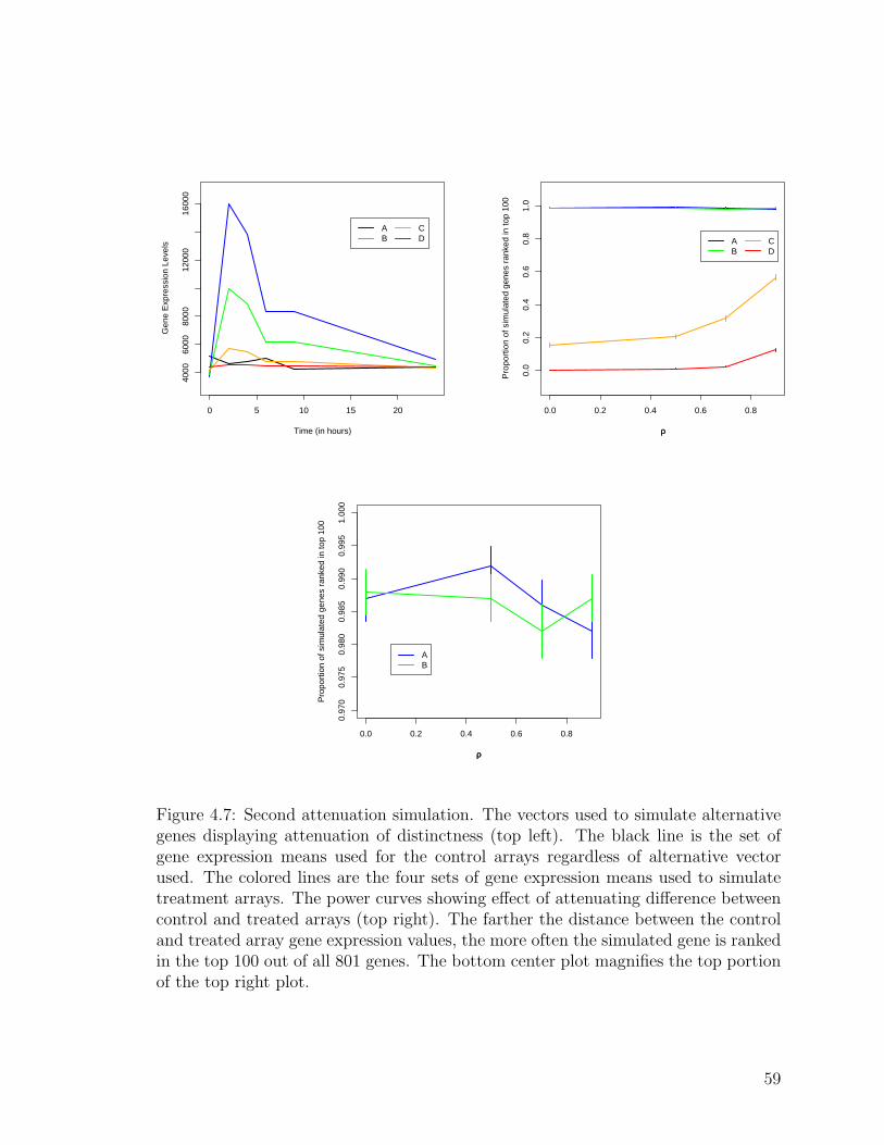
0 5 10 15 20

4000

6000

8000

1200

016

000

Time (in hours)

Gen

e E

xpre

ssio

n Le

vels

AB

CD

0.0 0.2 0.4 0.6 0.8

0.0

0.2

0.4

0.6

0.8

1.0

ρρ

Pro

port

ion

of s

imul

ated

gen

es r

anke

d in

top

100

AB

CD

0.0 0.2 0.4 0.6 0.8

0.97

00.

975

0.98

00.

985

0.99

00.

995

1.00

0

ρρ

Pro

port

ion

of s

imul

ated

gen

es r

anke

d in

top

100

AB

Figure 4.7: Second attenuation simulation. The vectors used to simulate alternativegenes displaying attenuation of distinctness (top left). The black line is the set ofgene expression means used for the control arrays regardless of alternative vectorused. The colored lines are the four sets of gene expression means used to simulatetreatment arrays. The power curves showing effect of attenuating difference betweencontrol and treated arrays (top right). The farther the distance between the controland treated array gene expression values, the more often the simulated gene is rankedin the top 100 out of all 801 genes. The bottom center plot magnifies the top portionof the top right plot.

59

Figure 4.8 shows the boxplots corresponding to the four treated vectors in

Figure 4.7. The data used to construct this plot are found in Table B.7. Plot A

corresponds to the original treated vector, plot B corresponds to the green vector,

plot C corresponds to the orange line, and plot D corresponds to the red line. As in

Figure 4.6, we see that as the genes become less significant, the boxplots have longer

tails and wider interquartile ranges.

60

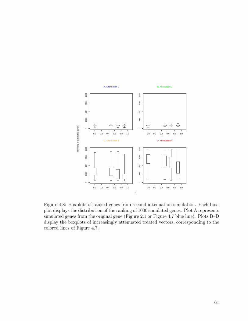
0.0 0.2 0.4 0.6 0.8 1.0

020

040

060

080

0

0.0 0.2 0.4 0.6 0.8 1.0

020

040

060

080

0

0.0 0.2 0.4 0.6 0.8 1.0

020

040

060

080

0

0.0 0.2 0.4 0.6 0.8 1.0

020

040

060

080

0

Ran

king

of s

imul

ated

gen

es

ρρ

A. Attenuation 1 B. Attenuation 2

C. Attenuation 3 D. Attenuation 4

Figure 4.8: Boxplots of ranked genes from second attenuation simulation. Each box-plot displays the distribution of the ranking of 1000 simulated genes. Plot A representssimulated genes from the original gene (Figure 2.1 or Figure 4.7 blue line). Plots B–Ddisplay the boxplots of increasingly attenuated treated vectors, corresponding to thecolored lines of Figure 4.7.

61

5. EVALUATING GENE EXPRESSION ANALYSES

THROUGH SIMULATION STUDIES

The results from the Storey method simulation provide insight into the Storey

method, the endotoxin data, and the way the method and data interact. In summary,

the following was found through the simulation.

In the endotoxin data set, the dominating pattern among treated arrays is to

start at normal expression levels, drop to low expression levels immediately following

treatment, and come back to normal expression levels by 24 hours past treatment.

Occasionally, a gene follows the opposite pattern—increase in expression following

treatment, then drop down to normal expression levels soon after. The study shows

the Storey method is very sensitive to this type of differential expression, as it de-

tects differences as small as 2000 gene expression units between control and treated

arrays approximately 70% of the time. The endotoxin data estimated ρ as 0.7 and

σ2 as approximately 250,000 gene expression units. As ρ increases to 0.9, artificial

significance is seen in null genes; however, at 0.7, the inflation in significance is not

present among null genes. Changing the variance had some slight effects, but these

effects were only detectable when the gene fell in the grey area between significance

and non-significance.

The specificity of these results to the data and method make them of little

interest to a researcher with other data and analysis methods; however, the process

that produced these results is enlightening and generalizable to any research situ-

ation. The numerical data produced by microarray experiments is relative to the

details of the experiment. While a surrogate of the quantity of RNA transcripts,

gene expression measurements do not represent an empirical quantity within the cell.

They are merely a surrogate value to provide a level of expression compared to other

62

genes. The interpretation of these artificial units is dependent on the type of array

being used, how the arrays were prepared, and the other arrays in the sample. Array

normalization can help make results comparable between slides, but the researcher is

still unsure what “significant” really entails. The end result of a microarray analysis

is a list of genes deemed significant by the method used; however, this information

rarely encompasses everything the researcher is interested in. What types of genes

are being called significant? What patterns are detected by this method? At what

point does a gene fall on the line between significant and non-significant? These are

all questions that can be answered by this simulation study.

The spike-in approach, developed to validate levels on an array, provides the

inspiration for the technique used in this simulation. Spiked genes—genes artificially

added to but not naturally found in the sample—are added in known quantities,

thereby providing a reference for the experimental results. Similarly, this simulation-

based approach adds a single gene with known features to an existing data set. By

observing the significance levels of the known gene, the researcher can have a better

idea of what types of genes the method is finding to be significant and to which gene

features the method is most sensitive.

Using the steps outlined by the endotoxin example, one can analyze the conse-

quences of using any analysis methods on any gene expression data. Although this

process may seem tedious and time consuming, the process used for the endotoxin

example can be modified to fit nearly any gene expression analysis. These steps are:

(1) Determine patterns of interest in the data. These patterns may be found by

examining dominant clusters, or they may be chosen by the researcher based

on knowledge from previous studies.

(2) Estimate reasonable parameter values. The endotoxin example used the

study’s data to estimate starting values for parameters such as µ, ρ, and

σ2, but one could use historical data to find these values as well.

63

(3) Generate a single gene to append to an existing data set. This example as-

sumes that a new gene is normally distributed with a spatial power correlation

structure; however, if another distribution seems better suited to the data,

these parameters can be easily modified.

(4) Analyze the outcome of changing features of the simulated gene. This simu-

lation study investigated the effects of changing µ, ρ, σ2, and the difference

between control and treated arrays. The choice of what to manipulate should

be made based on the data type and research question(s).

These steps, modified to fit a particular combination of method and data, will

help a researcher understand what significance involves and how to better interpret

the raw analysis results.

Future research could not only investigate features of the data, but could look

into aspects of the method as well. For instance, this method provided options to

be chosen by the user such as spline type (polynomial or natural cubic), number of

knots, and number of bootstrap iterations. Adjusting these arbitrary measures may

alter the method’s specificity to different gene expression patterns.

64

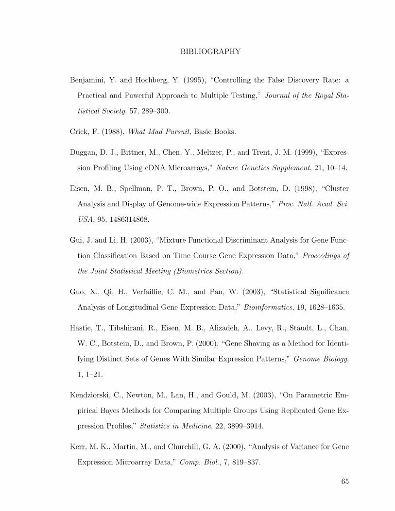
BIBLIOGRAPHY

Benjamini, Y. and Hochberg, Y. (1995), “Controlling the False Discovery Rate: a

Practical and Powerful Approach to Multiple Testing,” Journal of the Royal Sta-

tistical Society, 57, 289–300.

Crick, F. (1988), What Mad Pursuit, Basic Books.

Duggan, D. J., Bittner, M., Chen, Y., Meltzer, P., and Trent, J. M. (1999), “Expres-

sion Profiling Using cDNA Microarrays,” Nature Genetics Supplement, 21, 10–14.

Eisen, M. B., Spellman, P. T., Brown, P. O., and Botstein, D. (1998), “Cluster

Analysis and Display of Genome-wide Expression Patterns,” Proc. Natl. Acad. Sci.

USA, 95, 1486314868.

Gui, J. and Li, H. (2003), “Mixture Functional Discriminant Analysis for Gene Func-

tion Classification Based on Time Course Gene Expression Data,” Proceedings of

the Joint Statistical Meeting (Biometrics Section).

Guo, X., Qi, H., Verfaillie, C. M., and Pan, W. (2003), “Statistical Significance

Analysis of Longitudinal Gene Expression Data,” Bioinformatics, 19, 1628–1635.

Hastie, T., Tibshirani, R., Eisen, M. B., Alizadeh, A., Levy, R., Staudt, L., Chan,

W. C., Botstein, D., and Brown, P. (2000), “Gene Shaving as a Method for Identi-

fying Distinct Sets of Genes With Similar Expression Patterns,” Genome Biology,

1, 1–21.

Kendziorski, C., Newton, M., Lan, H., and Gould, M. (2003), “On Parametric Em-

pirical Bayes Methods for Comparing Multiple Groups Using Replicated Gene Ex-

pression Profiles,” Statistics in Medicine, 22, 3899–3914.

Kerr, M. K., Martin, M., and Churchill, G. A. (2000), “Analysis of Variance for Gene

Expression Microarray Data,” Comp. Biol., 7, 819–837.

65

Lodish, H., Berk, A., Zipursky, S. L., Matsudaira, P., Baltimore, D., and Darnell, J.

(2000), Molecular Cell Biology, W.H. Freeman and Company, 4th ed.

Luan, Y. and Li, H. (2004), “Model-based Methods for Identifying Periodically Ex-

pressed Genes Based on Time Course Microarray Gene Expression Data,” Bioin-

formatics, 20, 332–339.

Maddox, J. (2003), “How Genius Can Smooth the Road to Publication,” Nature, 426.

Mortensen, R. M. (1993), “Double Knockouts. Production of Mutant Cell Lines in

Cardiovascular Research,” Hypertension, 22, 646–651.

Muller, H.-J. and Roder, T. (2006), Microarrays, Elsevier Academic Press.

Parmigiani, G., Garrett, E. S., Irizarry, R. A., and Zeger, S. L. (eds.) (2003), The

Analysis of Gene Expression Data: Methods and Software, Springer.

Pollard, K. S. and van der Laan, M. J. (2002a), “Statistical Inference for Simultaneous

Clustering of Gene Expression Data,” Mathematical Biosciences, 176, 99–121.

Simon, R. M., Korn, E. L., McShane, L. M., Radmacher, M. D., Wright, G. W., and

Zhao, Y. (2003), Design and Analysis of DNA Microarray Investigations, Statistics

for Biology and Health, Springer.

Stasiak, A. (2003), “DNA’s Golden Jubilee,” EMBO reports, 4, 10251026.

Storey, J. D., Xiao, W., Leek, J. T., Thompkins, R. G., and David, R. W. (2005), “Sig-

nificance Analysis of Time Course Microarray Experiments,” PNAS, 102, 12837–

12842.

Tamayo, P., Slonim, D., Mesirov, J., Zhu, Q., Kitareewan, S., Dmitrovsky, E., Lander,

E. S., and Golub, T. R. (1999), “Interpreting Patterns of Gene Expression With

Self-organizing Maps: Methods and Application to Hematopoietic Differentiation,”

Proc. Natl. Acad. Sci. USA, 96, 29072912.

66

Tusher, V., Tibshirani, R., and Chu, G. (2001), “Significance Analysis of Microarrays

Applied to Ionizing Radiation Response,” Proc. Natl Acad. Sci. USA, 98, 5116–

5121.

van der Laan, M. J. and Pollard, K. S. (2003), “A New Algorithm for Hybrid Hier-

archical Clustering With Visualization and the Bootstrap,” Journal of Statistical

Planning and Inference, 117, 275–303.

Watson, J. (2001), The Double Helix: A Personal Account of the Discovery of the

Structure of DNA, Touchstone.

Watson, J. and Crick, F. (1953), “Molecular Structure of Nucleic Acids: A Structure

for Deoxyribose Nucleic Acid,” Nature, 171, 737–738.

Williams, R., Broman, K., Cheverud, J., Churchill, G., Hitzemann, R., Hunter, K.,

Mountz, J., Pomp, P., Reeves, R., Schalkwyk, L., and Threadgill, D. (2002), “A

Collaborative Cross for High-precision Complex Trait Analysis,” Tech. rep., Com-

plex Trait Consotium, www.complextrait.org/Workshop1.pdf.

Yuan, M., Kendziorski, C., Park, F., Porter, J. R., Hayes, K., and Bradfield, C. (2003),

“Hidden Markov Models for Microarray Time Course Data in Multiple Biological

Conditions,” Tech. Rep. 178, University of Wisconsin, Department of Biostatistics

and Medical Informatics, Madison, WI.

67

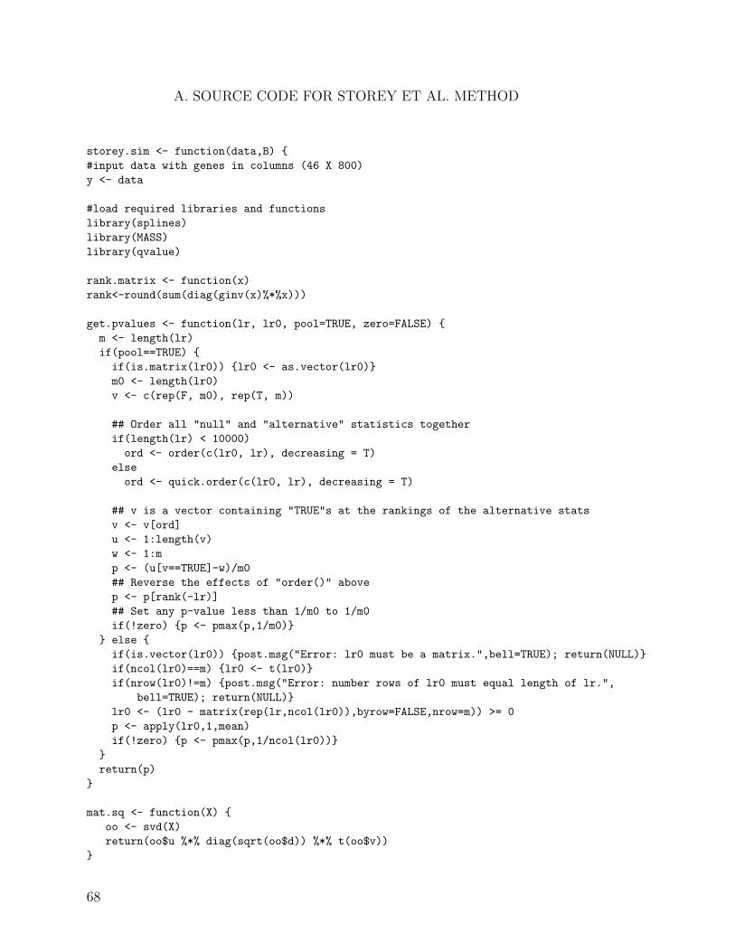
A. SOURCE CODE FOR STOREY ET AL. METHOD

storey.sim <- function(data,B) {#input data with genes in columns (46 X 800)y <- data

#load required libraries and functionslibrary(splines)library(MASS)library(qvalue)

rank.matrix <- function(x)rank<-round(sum(diag(ginv(x)%*%x)))

get.pvalues <- function(lr, lr0, pool=TRUE, zero=FALSE) {m <- length(lr)if(pool==TRUE) {if(is.matrix(lr0)) {lr0 <- as.vector(lr0)}m0 <- length(lr0)v <- c(rep(F, m0), rep(T, m))

## Order all "null" and "alternative" statistics togetherif(length(lr) < 10000)ord <- order(c(lr0, lr), decreasing = T)

elseord <- quick.order(c(lr0, lr), decreasing = T)

## v is a vector containing "TRUE"s at the rankings of the alternative statsv <- v[ord]u <- 1:length(v)w <- 1:mp <- (u[v==TRUE]-w)/m0## Reverse the effects of "order()" abovep <- p[rank(-lr)]## Set any p-value less than 1/m0 to 1/m0if(!zero) {p <- pmax(p,1/m0)}

} else {if(is.vector(lr0)) {post.msg("Error: lr0 must be a matrix.",bell=TRUE); return(NULL)}if(ncol(lr0)==m) {lr0 <- t(lr0)}if(nrow(lr0)!=m) {post.msg("Error: number rows of lr0 must equal length of lr.",

bell=TRUE); return(NULL)}lr0 <- (lr0 - matrix(rep(lr,ncol(lr0)),byrow=FALSE,nrow=m)) >= 0p <- apply(lr0,1,mean)if(!zero) {p <- pmax(p,1/ncol(lr0))}

}return(p)

}

mat.sq <- function(X) {oo <- svd(X)return(oo$u %*% diag(sqrt(oo$d)) %*% t(oo$v))

}

68

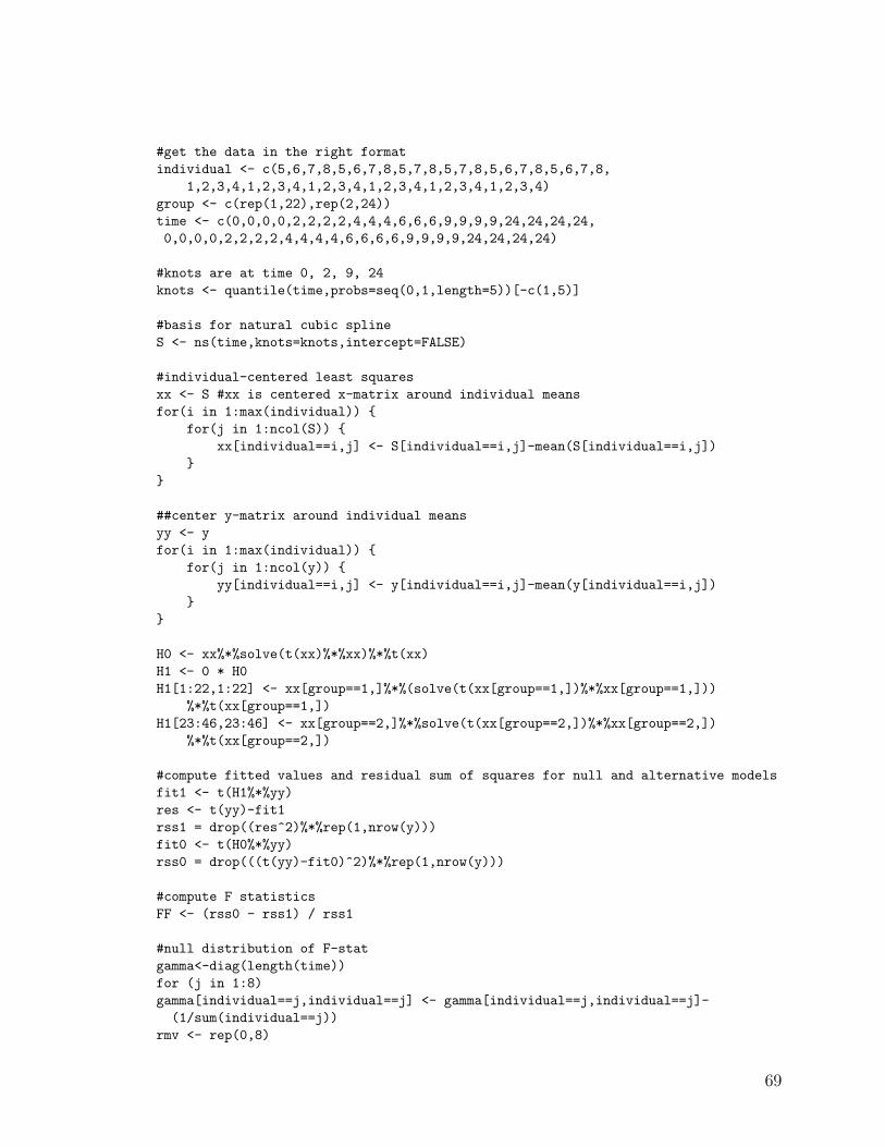
#get the data in the right formatindividual <- c(5,6,7,8,5,6,7,8,5,7,8,5,7,8,5,6,7,8,5,6,7,8,

1,2,3,4,1,2,3,4,1,2,3,4,1,2,3,4,1,2,3,4,1,2,3,4)group <- c(rep(1,22),rep(2,24))time <- c(0,0,0,0,2,2,2,2,4,4,4,6,6,6,9,9,9,9,24,24,24,24,0,0,0,0,2,2,2,2,4,4,4,4,6,6,6,6,9,9,9,9,24,24,24,24)

#knots are at time 0, 2, 9, 24knots <- quantile(time,probs=seq(0,1,length=5))[-c(1,5)]

#basis for natural cubic splineS <- ns(time,knots=knots,intercept=FALSE)

#individual-centered least squaresxx <- S #xx is centered x-matrix around individual meansfor(i in 1:max(individual)) {

for(j in 1:ncol(S)) {xx[individual==i,j] <- S[individual==i,j]-mean(S[individual==i,j])

}}

##center y-matrix around individual meansyy <- yfor(i in 1:max(individual)) {

for(j in 1:ncol(y)) {yy[individual==i,j] <- y[individual==i,j]-mean(y[individual==i,j])

}}

H0 <- xx%*%solve(t(xx)%*%xx)%*%t(xx)H1 <- 0 * H0H1[1:22,1:22] <- xx[group==1,]%*%(solve(t(xx[group==1,])%*%xx[group==1,]))

%*%t(xx[group==1,])H1[23:46,23:46] <- xx[group==2,]%*%solve(t(xx[group==2,])%*%xx[group==2,])

%*%t(xx[group==2,])

#compute fitted values and residual sum of squares for null and alternative modelsfit1 <- t(H1%*%yy)res <- t(yy)-fit1rss1 = drop((res^2)%*%rep(1,nrow(y)))fit0 <- t(H0%*%yy)rss0 = drop(((t(yy)-fit0)^2)%*%rep(1,nrow(y)))

#compute F statisticsFF <- (rss0 - rss1) / rss1

#null distribution of F-statgamma<-diag(length(time))for (j in 1:8)gamma[individual==j,individual==j] <- gamma[individual==j,individual==j]-(1/sum(individual==j))

rmv <- rep(0,8)

69

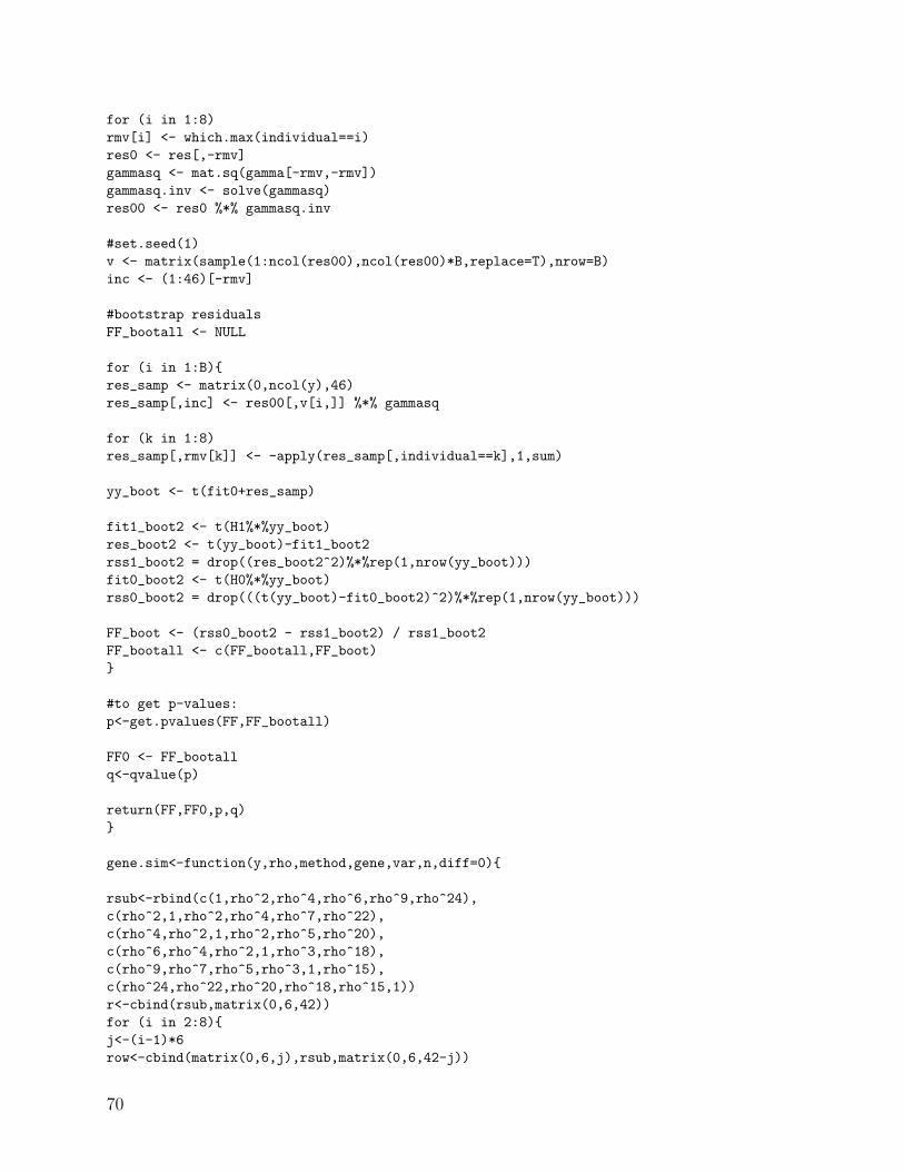
for (i in 1:8)rmv[i] <- which.max(individual==i)res0 <- res[,-rmv]gammasq <- mat.sq(gamma[-rmv,-rmv])gammasq.inv <- solve(gammasq)res00 <- res0 %*% gammasq.inv

#set.seed(1)v <- matrix(sample(1:ncol(res00),ncol(res00)*B,replace=T),nrow=B)inc <- (1:46)[-rmv]

#bootstrap residualsFF_bootall <- NULL

for (i in 1:B){res_samp <- matrix(0,ncol(y),46)res_samp[,inc] <- res00[,v[i,]] %*% gammasq

for (k in 1:8)res_samp[,rmv[k]] <- -apply(res_samp[,individual==k],1,sum)

yy_boot <- t(fit0+res_samp)

fit1_boot2 <- t(H1%*%yy_boot)res_boot2 <- t(yy_boot)-fit1_boot2rss1_boot2 = drop((res_boot2^2)%*%rep(1,nrow(yy_boot)))fit0_boot2 <- t(H0%*%yy_boot)rss0_boot2 = drop(((t(yy_boot)-fit0_boot2)^2)%*%rep(1,nrow(yy_boot)))

FF_boot <- (rss0_boot2 - rss1_boot2) / rss1_boot2FF_bootall <- c(FF_bootall,FF_boot)}

#to get p-values:p<-get.pvalues(FF,FF_bootall)

FF0 <- FF_bootallq<-qvalue(p)

return(FF,FF0,p,q)}

gene.sim<-function(y,rho,method,gene,var,n,diff=0){

rsub<-rbind(c(1,rho^2,rho^4,rho^6,rho^9,rho^24),c(rho^2,1,rho^2,rho^4,rho^7,rho^22),c(rho^4,rho^2,1,rho^2,rho^5,rho^20),c(rho^6,rho^4,rho^2,1,rho^3,rho^18),c(rho^9,rho^7,rho^5,rho^3,1,rho^15),c(rho^24,rho^22,rho^20,rho^18,rho^15,1))r<-cbind(rsub,matrix(0,6,42))for (i in 2:8){j<-(i-1)*6row<-cbind(matrix(0,6,j),rsub,matrix(0,6,42-j))

70

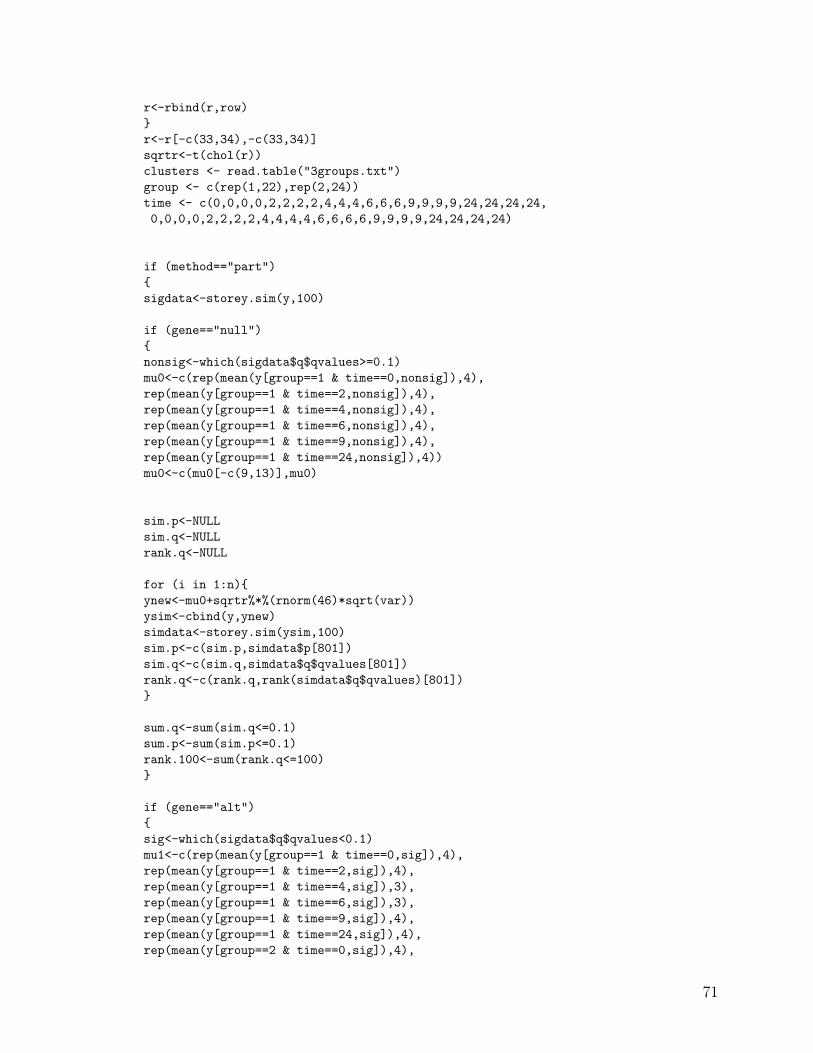
r<-rbind(r,row)}r<-r[-c(33,34),-c(33,34)]sqrtr<-t(chol(r))clusters <- read.table("3groups.txt")group <- c(rep(1,22),rep(2,24))time <- c(0,0,0,0,2,2,2,2,4,4,4,6,6,6,9,9,9,9,24,24,24,24,0,0,0,0,2,2,2,2,4,4,4,4,6,6,6,6,9,9,9,9,24,24,24,24)

if (method=="part"){sigdata<-storey.sim(y,100)

if (gene=="null"){nonsig<-which(sigdata$q$qvalues>=0.1)mu0<-c(rep(mean(y[group==1 & time==0,nonsig]),4),rep(mean(y[group==1 & time==2,nonsig]),4),rep(mean(y[group==1 & time==4,nonsig]),4),rep(mean(y[group==1 & time==6,nonsig]),4),rep(mean(y[group==1 & time==9,nonsig]),4),rep(mean(y[group==1 & time==24,nonsig]),4))mu0<-c(mu0[-c(9,13)],mu0)

sim.p<-NULLsim.q<-NULLrank.q<-NULL

for (i in 1:n){ynew<-mu0+sqrtr%*%(rnorm(46)*sqrt(var))ysim<-cbind(y,ynew)simdata<-storey.sim(ysim,100)sim.p<-c(sim.p,simdata$p[801])sim.q<-c(sim.q,simdata$q$qvalues[801])rank.q<-c(rank.q,rank(simdata$q$qvalues)[801])}

sum.q<-sum(sim.q<=0.1)sum.p<-sum(sim.p<=0.1)rank.100<-sum(rank.q<=100)}

if (gene=="alt"){sig<-which(sigdata$q$qvalues<0.1)mu1<-c(rep(mean(y[group==1 & time==0,sig]),4),rep(mean(y[group==1 & time==2,sig]),4),rep(mean(y[group==1 & time==4,sig]),3),rep(mean(y[group==1 & time==6,sig]),3),rep(mean(y[group==1 & time==9,sig]),4),rep(mean(y[group==1 & time==24,sig]),4),rep(mean(y[group==2 & time==0,sig]),4),

71

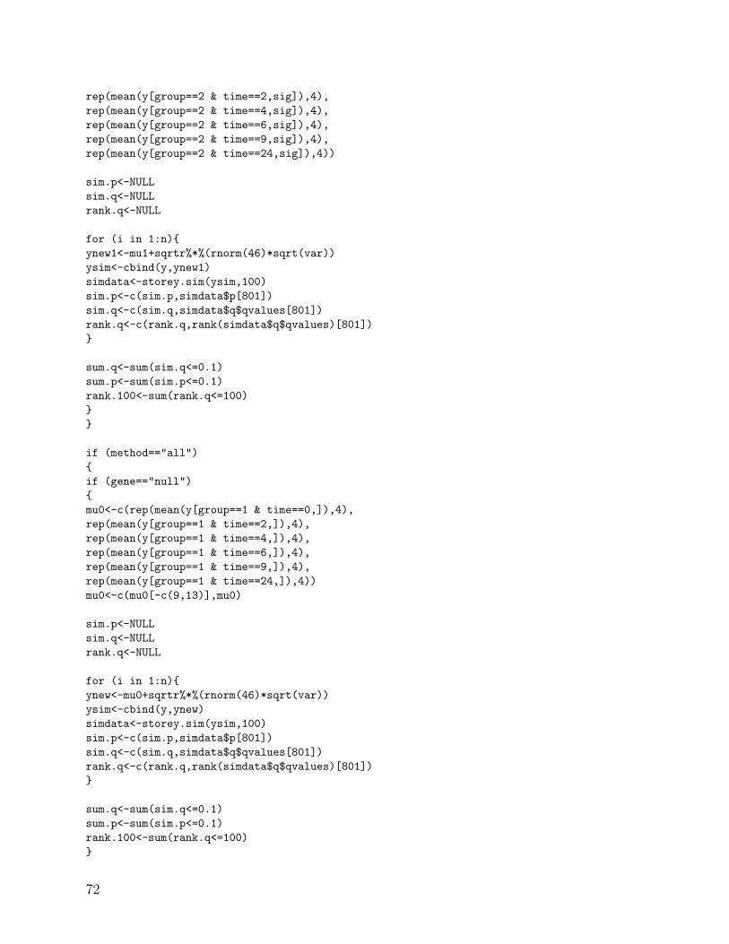
rep(mean(y[group==2 & time==2,sig]),4),rep(mean(y[group==2 & time==4,sig]),4),rep(mean(y[group==2 & time==6,sig]),4),rep(mean(y[group==2 & time==9,sig]),4),rep(mean(y[group==2 & time==24,sig]),4))

sim.p<-NULLsim.q<-NULLrank.q<-NULL

for (i in 1:n){ynew1<-mu1+sqrtr%*%(rnorm(46)*sqrt(var))ysim<-cbind(y,ynew1)simdata<-storey.sim(ysim,100)sim.p<-c(sim.p,simdata$p[801])sim.q<-c(sim.q,simdata$q$qvalues[801])rank.q<-c(rank.q,rank(simdata$q$qvalues)[801])}

sum.q<-sum(sim.q<=0.1)sum.p<-sum(sim.p<=0.1)rank.100<-sum(rank.q<=100)}}

if (method=="all"){if (gene=="null"){mu0<-c(rep(mean(y[group==1 & time==0,]),4),rep(mean(y[group==1 & time==2,]),4),rep(mean(y[group==1 & time==4,]),4),rep(mean(y[group==1 & time==6,]),4),rep(mean(y[group==1 & time==9,]),4),rep(mean(y[group==1 & time==24,]),4))mu0<-c(mu0[-c(9,13)],mu0)

sim.p<-NULLsim.q<-NULLrank.q<-NULL

for (i in 1:n){ynew<-mu0+sqrtr%*%(rnorm(46)*sqrt(var))ysim<-cbind(y,ynew)simdata<-storey.sim(ysim,100)sim.p<-c(sim.p,simdata$p[801])sim.q<-c(sim.q,simdata$q$qvalues[801])rank.q<-c(rank.q,rank(simdata$q$qvalues)[801])}

sum.q<-sum(sim.q<=0.1)sum.p<-sum(sim.p<=0.1)rank.100<-sum(rank.q<=100)}

72

if (gene=="alt"){mu1<-c(rep(mean(y[group==1 & time==0,]),4),rep(mean(y[group==1 & time==2,]),4),rep(mean(y[group==1 & time==4,]),3),rep(mean(y[group==1 & time==6,]),3),rep(mean(y[group==1 & time==9,]),4),rep(mean(y[group==1 & time==24,]),4),rep(mean(y[group==2 & time==0,]),4),rep(mean(y[group==2 & time==2,]),4),rep(mean(y[group==2 & time==4,]),4),rep(mean(y[group==2 & time==6,]),4),rep(mean(y[group==2 & time==9,]),4),rep(mean(y[group==2 & time==24,]),4))

sim.p<-NULLsim.q<-NULLrank.q<-NULL

for (i in 1:n){ynew1<-mu1+sqrtr%*%(rnorm(46)*sqrt(var))ysim<-cbind(y,ynew1)simdata<-storey.sim(ysim,100)sim.p<-c(sim.p,simdata$p[801])sim.q<-c(sim.q,simdata$q$qvalues[801])rank.q<-c(rank.q,rank(simdata$q$qvalues)[801])}

sum.q<-sum(sim.q<=0.1)sum.p<-sum(sim.p<=0.1)rank.100<-sum(rank.q<=100)}}

if (method=="group"){if (gene=="null"){mu0<-c(rep(mean(y[group==1 & time==0,clusters[,2]==1]),4),rep(mean(y[group==1 & time==2,clusters[,2]==1]),4),rep(mean(y[group==1 & time==4,clusters[,2]==1]),3),rep(mean(y[group==1 & time==6,clusters[,2]==1]),3),rep(mean(y[group==1 & time==9,clusters[,2]==1]),4),rep(mean(y[group==1 & time==24,clusters[,2]==1]),4))mu0<-c(mu0[-c(9,13)],mu0)

sim.p<-NULLsim.q<-NULLrank.q<-NULL

for (i in 1:n){ynew<-mu0+sqrtr%*%(rnorm(46)*sqrt(var))ysim<-cbind(y,ynew)simdata<-storey.sim(ysim,100)

73

sim.p<-c(sim.p,simdata$p[801])sim.q<-c(sim.q,simdata$q$qvalues[801])rank.q<-c(rank.q,rank(simdata$q$qvalues)[801])}

sum.q<-sum(sim.q<=0.1)sum.p<-sum(sim.p<=0.1)rank.100<-sum(rank.q<=100)}if (gene=="alt"){mu1<-c(rep(mean(y[group==1 & time==0,clusters[,2]==3])-diff,4),rep(mean(y[group==1 & time==2,clusters[,2]==3])-diff,4),rep(mean(y[group==1 & time==4,clusters[,2]==3])-diff,3),rep(mean(y[group==1 & time==6,clusters[,2]==3])-diff,3),rep(mean(y[group==1 & time==9,clusters[,2]==3])-diff,4),rep(mean(y[group==1 & time==24,clusters[,2]==3])-diff,4),rep(mean(y[group==2 & time==0,clusters[,2]==3]),4),rep(mean(y[group==2 & time==2,clusters[,2]==3]),4),rep(mean(y[group==2 & time==4,clusters[,2]==3]),4),rep(mean(y[group==2 & time==6,clusters[,2]==3]),4),rep(mean(y[group==2 & time==9,clusters[,2]==3]),4),rep(mean(y[group==2 & time==24,clusters[,2]==3]),4))

sim.p<-NULLsim.q<-NULLrank.q<-NULL

for (i in 1:n){ynew1<-mu1+sqrtr%*%(rnorm(46)*sqrt(var))ysim<-cbind(y,ynew1)simdata<-storey.sim(ysim,100)sim.p<-c(sim.p,simdata$p[801])sim.q<-c(sim.q,simdata$q$qvalues[801])rank.q<-c(rank.q,rank(simdata$q$qvalues)[801])}

sum.q<-sum(sim.q<=0.1)sum.p<-sum(sim.p<=0.1)rank.100<-sum(rank.q<=100)}}

if (method=="curve"){if (gene=="alt"){mu.clust<-c(rep(mean(y[group==1 & time==0,clusters[,2]==3]),4),rep(mean(y[group==1 & time==2,clusters[,2]==3]),4),rep(mean(y[group==1 & time==4,clusters[,2]==3]),3),rep(mean(y[group==1 & time==6,clusters[,2]==3]),3),rep(mean(y[group==1 & time==9,clusters[,2]==3]),4),

74

rep(mean(y[group==1 & time==24,clusters[,2]==3]),4),rep(mean(y[group==2 & time==0,clusters[,2]==3]),4),rep(mean(y[group==2 & time==2,clusters[,2]==3]),4),rep(mean(y[group==2 & time==4,clusters[,2]==3]),4),rep(mean(y[group==2 & time==6,clusters[,2]==3]),4),rep(mean(y[group==2 & time==9,clusters[,2]==3]),4),rep(mean(y[group==2 & time==24,clusters[,2]==3]),4))

mu1<-c(mu.clust[1:22],(mu.clust[23:46]-17000)*.5+20000)mu2<-c(mu.clust[1:22],(mu1[23:46]-20000)*.5+23000)mu3<-c(mu.clust[1:22],(mu2[23:46]-23000)*.75+25000)mu4<-c(mu.clust[1:22],(mu3[23:46]-25000)*.75+25500)mu5<-c(mu.clust[1:22],(mu4[23:46]-25500)*.75+26000)

if (diff==0) mu<-mu.clustif (diff==1) mu<-mu1if (diff==2) mu<-mu2if (diff==3) mu<-mu3if (diff==4) mu<-mu4if (diff==5) mu<-mu5

sim.p<-NULLsim.q<-NULLrank.q<-NULL

for (i in 1:n){ynew1<-mu+sqrtr%*%(rnorm(46)*sqrt(var))ysim<-cbind(y,ynew1)simdata<-storey.sim(ysim,100)sim.p<-c(sim.p,simdata$p[801])sim.q<-c(sim.q,simdata$q$qvalues[801])rank.q<-c(rank.q,rank(simdata$q$qvalues)[801])}

sum.q<-sum(sim.q<=0.1)sum.p<-sum(sim.p<=0.1)rank.100<-sum(rank.q<=100)}}

if (method=="230"){if (gene=="alt"){mu.230<-c(rep(mean(y[group==1 & time==0,230]),4),rep(mean(y[group==1 & time==2,230]),4),rep(mean(y[group==1 & time==4,230]),3),rep(mean(y[group==1 & time==6,230]),3),rep(mean(y[group==1 & time==9,230]),4),rep(mean(y[group==1 & time==24,230]),4),rep(mean(y[group==2 & time==0,230]),4),rep(mean(y[group==2 & time==2,230]),4),

75

rep(mean(y[group==2 & time==4,230]),4),rep(mean(y[group==2 & time==6,230]),4),rep(mean(y[group==2 & time==9,230]),4),rep(mean(y[group==2 & time==24,230]),4))

mu1<-c(mu.230[1:22],(mu.230[23:46]-10000)*.5+7000)mu2<-c(mu.230[1:22],(mu1[23:46]-7000)*.25+5000)mu3<-c(mu.230[1:22],(mu2[23:46]-5000)*.1+4500)

if (diff==0) mu<-mu.230if (diff==1) mu<-mu1if (diff==2) mu<-mu2if (diff==3) mu<-mu3

sim.p<-NULLsim.q<-NULLrank.q<-NULL

for (i in 1:n){ynew1<-mu+sqrtr%*%(rnorm(46)*sqrt(var))ysim<-cbind(y,ynew1)simdata<-storey.sim(ysim,100)sim.p<-c(sim.p,simdata$p[801])sim.q<-c(sim.q,simdata$q$qvalues[801])rank.q<-c(rank.q,rank(simdata$q$qvalues)[801])}

sum.q<-sum(sim.q<=0.1)sum.p<-sum(sim.p<=0.1)rank.100<-sum(rank.q<=100)}}return(sum.q,sum.p,rank.q,rank.100)}

76

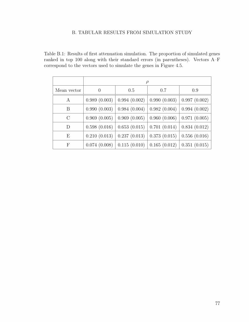
B. TABULAR RESULTS FROM SIMULATION STUDY

Table B.1: Results of first attenuation simulation. The proportion of simulated genesranked in top 100 along with their standard errors (in parentheses). Vectors A–Fcorrespond to the vectors used to simulate the genes in Figure 4.5.

ρ

Mean vector 0 0.5 0.7 0.9

A 0.989 (0.003) 0.994 (0.002) 0.990 (0.003) 0.997 (0.002)

B 0.990 (0.003) 0.984 (0.004) 0.982 (0.004) 0.994 (0.002)

C 0.969 (0.005) 0.969 (0.005) 0.960 (0.006) 0.971 (0.005)

D 0.598 (0.016) 0.653 (0.015) 0.701 (0.014) 0.834 (0.012)

E 0.210 (0.013) 0.237 (0.013) 0.373 (0.015) 0.556 (0.016)

F 0.074 (0.008) 0.115 (0.010) 0.165 (0.012) 0.351 (0.015)

77

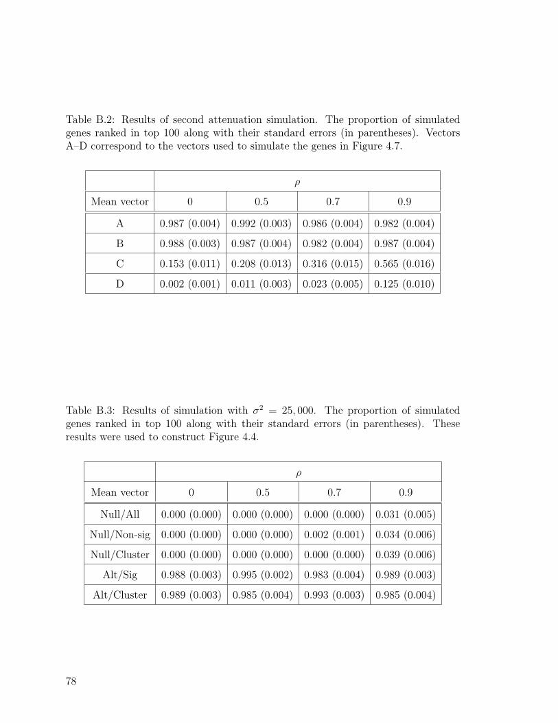
Table B.2: Results of second attenuation simulation. The proportion of simulatedgenes ranked in top 100 along with their standard errors (in parentheses). VectorsA–D correspond to the vectors used to simulate the genes in Figure 4.7.

ρ

Mean vector 0 0.5 0.7 0.9

A 0.987 (0.004) 0.992 (0.003) 0.986 (0.004) 0.982 (0.004)

B 0.988 (0.003) 0.987 (0.004) 0.982 (0.004) 0.987 (0.004)

C 0.153 (0.011) 0.208 (0.013) 0.316 (0.015) 0.565 (0.016)

D 0.002 (0.001) 0.011 (0.003) 0.023 (0.005) 0.125 (0.010)

Table B.3: Results of simulation with σ2 = 25, 000. The proportion of simulatedgenes ranked in top 100 along with their standard errors (in parentheses). Theseresults were used to construct Figure 4.4.

ρ

Mean vector 0 0.5 0.7 0.9

Null/All 0.000 (0.000) 0.000 (0.000) 0.000 (0.000) 0.031 (0.005)

Null/Non-sig 0.000 (0.000) 0.000 (0.000) 0.002 (0.001) 0.034 (0.006)

Null/Cluster 0.000 (0.000) 0.000 (0.000) 0.000 (0.000) 0.039 (0.006)

Alt/Sig 0.988 (0.003) 0.995 (0.002) 0.983 (0.004) 0.989 (0.003)

Alt/Cluster 0.989 (0.003) 0.985 (0.004) 0.993 (0.003) 0.985 (0.004)

78

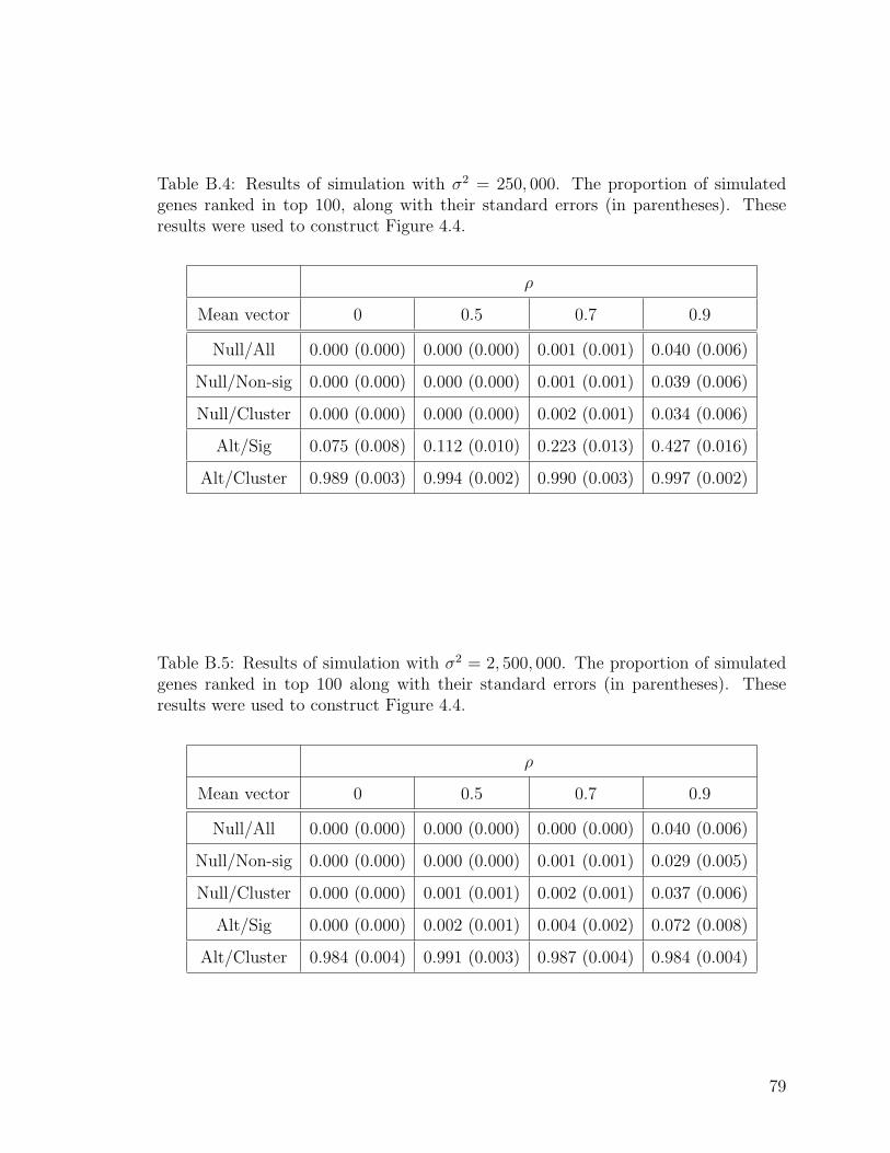
Table B.4: Results of simulation with σ2 = 250, 000. The proportion of simulatedgenes ranked in top 100, along with their standard errors (in parentheses). Theseresults were used to construct Figure 4.4.

ρ

Mean vector 0 0.5 0.7 0.9

Null/All 0.000 (0.000) 0.000 (0.000) 0.001 (0.001) 0.040 (0.006)

Null/Non-sig 0.000 (0.000) 0.000 (0.000) 0.001 (0.001) 0.039 (0.006)

Null/Cluster 0.000 (0.000) 0.000 (0.000) 0.002 (0.001) 0.034 (0.006)

Alt/Sig 0.075 (0.008) 0.112 (0.010) 0.223 (0.013) 0.427 (0.016)

Alt/Cluster 0.989 (0.003) 0.994 (0.002) 0.990 (0.003) 0.997 (0.002)

Table B.5: Results of simulation with σ2 = 2, 500, 000. The proportion of simulatedgenes ranked in top 100 along with their standard errors (in parentheses). Theseresults were used to construct Figure 4.4.

ρ

Mean vector 0 0.5 0.7 0.9

Null/All 0.000 (0.000) 0.000 (0.000) 0.000 (0.000) 0.040 (0.006)

Null/Non-sig 0.000 (0.000) 0.000 (0.000) 0.001 (0.001) 0.029 (0.005)

Null/Cluster 0.000 (0.000) 0.001 (0.001) 0.002 (0.001) 0.037 (0.006)

Alt/Sig 0.000 (0.000) 0.002 (0.001) 0.004 (0.002) 0.072 (0.008)

Alt/Cluster 0.984 (0.004) 0.991 (0.003) 0.987 (0.004) 0.984 (0.004)

79

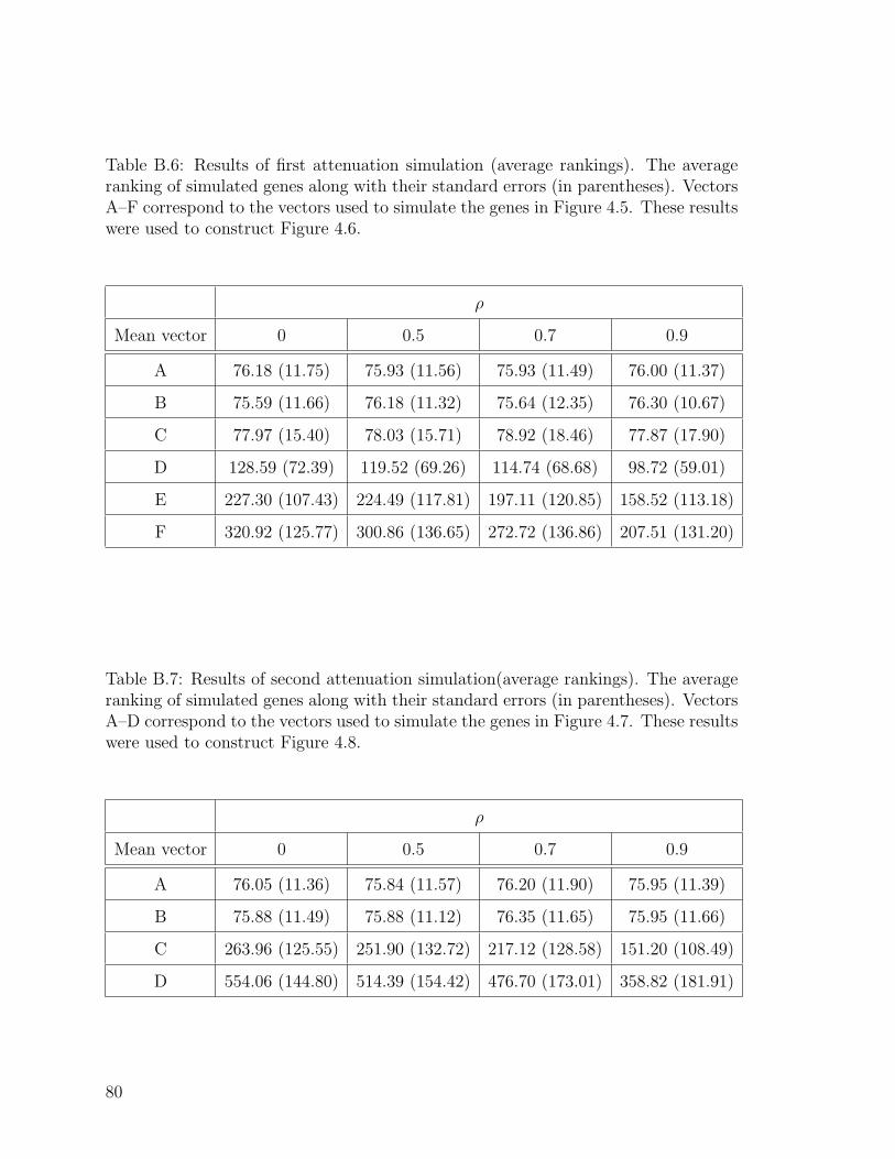
Table B.6: Results of first attenuation simulation (average rankings). The averageranking of simulated genes along with their standard errors (in parentheses). VectorsA–F correspond to the vectors used to simulate the genes in Figure 4.5. These resultswere used to construct Figure 4.6.

ρ

Mean vector 0 0.5 0.7 0.9

A 76.18 (11.75) 75.93 (11.56) 75.93 (11.49) 76.00 (11.37)

B 75.59 (11.66) 76.18 (11.32) 75.64 (12.35) 76.30 (10.67)

C 77.97 (15.40) 78.03 (15.71) 78.92 (18.46) 77.87 (17.90)

D 128.59 (72.39) 119.52 (69.26) 114.74 (68.68) 98.72 (59.01)

E 227.30 (107.43) 224.49 (117.81) 197.11 (120.85) 158.52 (113.18)

F 320.92 (125.77) 300.86 (136.65) 272.72 (136.86) 207.51 (131.20)

Table B.7: Results of second attenuation simulation(average rankings). The averageranking of simulated genes along with their standard errors (in parentheses). VectorsA–D correspond to the vectors used to simulate the genes in Figure 4.7. These resultswere used to construct Figure 4.8.

ρ

Mean vector 0 0.5 0.7 0.9

A 76.05 (11.36) 75.84 (11.57) 76.20 (11.90) 75.95 (11.39)

B 75.88 (11.49) 75.88 (11.12) 76.35 (11.65) 75.95 (11.66)

C 263.96 (125.55) 251.90 (132.72) 217.12 (128.58) 151.20 (108.49)

D 554.06 (144.80) 514.39 (154.42) 476.70 (173.01) 358.82 (181.91)

80

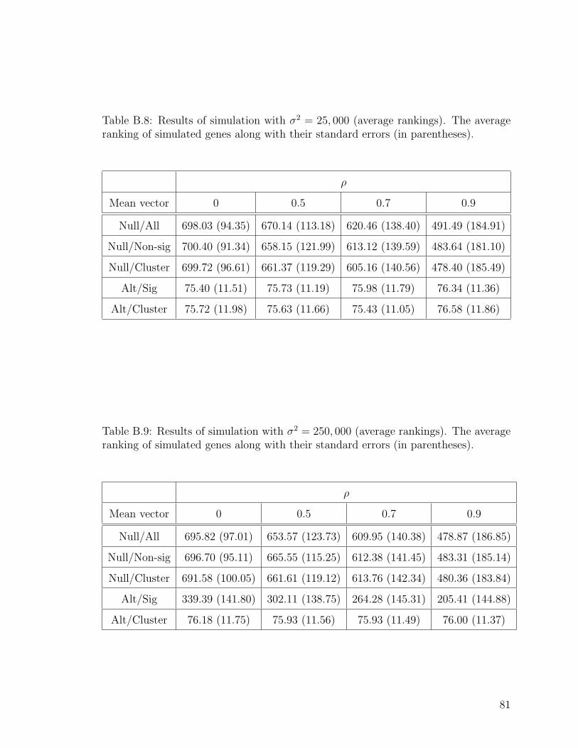
Table B.8: Results of simulation with σ2 = 25, 000 (average rankings). The averageranking of simulated genes along with their standard errors (in parentheses).

ρ

Mean vector 0 0.5 0.7 0.9

Null/All 698.03 (94.35) 670.14 (113.18) 620.46 (138.40) 491.49 (184.91)

Null/Non-sig 700.40 (91.34) 658.15 (121.99) 613.12 (139.59) 483.64 (181.10)

Null/Cluster 699.72 (96.61) 661.37 (119.29) 605.16 (140.56) 478.40 (185.49)

Alt/Sig 75.40 (11.51) 75.73 (11.19) 75.98 (11.79) 76.34 (11.36)

Alt/Cluster 75.72 (11.98) 75.63 (11.66) 75.43 (11.05) 76.58 (11.86)

Table B.9: Results of simulation with σ2 = 250, 000 (average rankings). The averageranking of simulated genes along with their standard errors (in parentheses).

ρ

Mean vector 0 0.5 0.7 0.9

Null/All 695.82 (97.01) 653.57 (123.73) 609.95 (140.38) 478.87 (186.85)

Null/Non-sig 696.70 (95.11) 665.55 (115.25) 612.38 (141.45) 483.31 (185.14)

Null/Cluster 691.58 (100.05) 661.61 (119.12) 613.76 (142.34) 480.36 (183.84)

Alt/Sig 339.39 (141.80) 302.11 (138.75) 264.28 (145.31) 205.41 (144.88)

Alt/Cluster 76.18 (11.75) 75.93 (11.56) 75.93 (11.49) 76.00 (11.37)

81

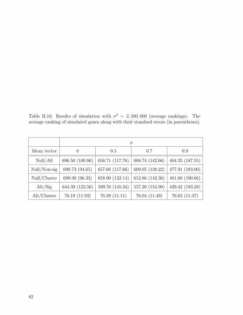
Table B.10: Results of simulation with σ2 = 2, 500, 000 (average rankings). Theaverage ranking of simulated genes along with their standard errors (in parentheses).

ρ

Mean vector 0 0.5 0.7 0.9

Null/All 696.50 (100.86) 656.71 (117.76) 608.74 (142.66) 484.35 (187.55)

Null/Non-sig 698.73 (94.65) 657.66 (117.66) 609.05 (138.22) 477.91 (183.00)

Null/Cluster 699.39 (96.33) 658.90 (122.14) 612.86 (142.36) 481.60 (190.66)

Alt/Sig 644.39 (122.56) 599.76 (145.34) 557.20 (154.90) 439.42 (193.28)

Alt/Cluster 76.19 (11.93) 76.38 (11.11) 76.04 (11.49) 76.63 (11.37)

82