1

AMSE JOURNALS-2016-Series: Advances D; Vol. 21; N° 1; pp 1-18

Submitted Feb. 2016; Revised April 15, 2016, Accepted May 15, 2016

A Simultaneous Solution of the Gilbert Equation

and its equivalent Landau-Lifshitz-Gilbert Equation

*Messaoud Boufligha, **Sebti Boukhtache

* Department of Electrical Engineering, Faculty of Technology, University of Batna

Rue Chahid Med El-Hadi Boukhlouf, 05000, Batna, Algeria (messaoud.boufligha@yahoo.fr)

** Department of Electrical engineering, Faculty of technology, University of Batna

Rue Chahid Med El-Hadi Boukhlouf, 05000, Batna, Algeria (sebti_boukhtache@yahoo.fr)

Abstract

We present an attempt of a development of at home FORTRAN and Matlab micromagnetic

codes based respectively on solving the Gilbert and the Landau-Lifshitz-Gilbert (LLG) equations.

These equations are respectively time-integrated by the Cash-Karp-Runge-Kutta (CKRK) algorithm

with a customized number of trials (NT) in adapting step size and the standard Runge-Kutta (RK)

method. In space, the finite difference method is employed. The previous tools are used in the

simulations of the magnetization reversal in a Permalloy thin film, with thermal effects. These

simulations have confirmed that the magnetization reversal is depended on the cell size. The (NT)

has an impact on the computational time at reduced size. The results given by the solvers showed a

slight discrepancy. The validation of our programs is limited to ensuring the correctness of the

implementation of the above equations and the employed time-integration methods. For this

purpose, the Larmor-precession frequency test is used.

Key words

Thin film; micromagnetic codes; magnetization reversal; thermal effects.

1. Introduction

Ferromagnetic thin films have become important because of their presence in sensors, read/write

heads and storage devices. Furthermore, miocromagnetic calculation has evolved for optimizing

properties of magnetic structures on the nano and micro scales. It is well known that by combining

the classical micromagnetic theory with dynamic descriptions of magnetization, one can

2

simulate the complete magnetization process. This leads to the solution of the Gilbert or its

equivalent (LLG) equations which allow us to get information at time-spatial scales that are not

accessible experimentally. Unfortunately, these equations have a non linear character. They can

only be treated with numerical methods. It is interesting to note that several groups have developed

their own versions of codes, based on solving the above equations. Some of them are free, such as

Magpar [1], Nmag [2], OOMMF [3], some are commercial, such as LLGsimilator[4], Micromagus

[5]. Much effort has been focused on how to include thermal effects in the analysis of the

magnetization process. Pioneering investigations were carried out by Neel [6] who studied the

influence of thermal fluctuations on the magnetization of fine ferromagnetic particles. Using the

Langevin dynamics, Brown [7] gave a first insight into magnetization reversal of a single-domain

particle by thermal fluctuations. He came up with the idea of adding a stochastic field to the

effective field in the micromagnetic equations. The use of the previous simulation packages is

influenced by many requirements as well as the necessary user license, scripting support, the chosen

discretization method, the programming language and interface libraries. Recently, researchers have

shown increasing interest in the coupling between magnetism and other effects such as conduction,

thermal and magnetoelastic effects. Thus, the flexibility of simulation tools becomes a necessity. In

this paper, we present an attempt of a development of customized FORTRAN and Matlab codes.

The development is based on solving the Gilbert and its equivalent (LLG) equations. They are

respectively time-integrated using the Cash-Karp-Runge-Kutta (CKRK) algorithm with a

customized number of trials (NT) in adapting time step size control and the standard (RK) method

[8,9]. In space, they are discretized by the finite difference method which helps in implementing the

Fast Fourier Transform (FFT) technique for demagnetizing field calculations [10]. The analysis of

the magnetization reversal at finite temperature in a Permalloy thin film, Ni80Fe20 using our own

developed tools is achieved. To validate our solvers, we are interested in this paper only to check

the correctness of the implementation of the two equivalent equations and the employed time-

integration methods by the use of the Larmor-precession frequency test. The present paper is

organized as follows: after the introduction in section 1, some details about the used micromagnetic

model and the simulation algorithm are presented in section 2. The simulation results, discussion,

the partial validation are summarized in section 3. The paper is closed with conclusions.

2. Model and simulation details

Theoretical micromagnetics as founded by W. F. Brown allows us to evaluate the total magnetic

free energy, Etot, of any ferromagnetic body if geometry, material parameters are known. It is the

sum of four energy terms

3

extdemanisexchtot EEEEE (1)

Where

Eexch is exchange energy: It is related to the formation of the domain wall,

Eanis is magnetocristalline energy: It is closely associated with the crystallographic directions

along which the magnetic moments are aligned,

Edem is magnetostatic energy: It originates from the long-range dipole-dipole interactions, and

Eext is the energy due to an external field: It forces the magnetization to become oriented in field

directions.

The analysis of the magnetization process in ferromagnetic thin films begins with the solution of

the micromagnetic equations. For static problems [11] the solution is given by

0 effHM (2)

Whereas, for dynamic problems, the solution is given by the Gilbert equation

dt

dMM

MHM

dt

dM

s

eff

(3)

Or its equivalent (LLG) equation

eff

s

eff HMMM

HMdt

dM

22 11

(4)

Where

M is the magnetic moment per unit volume,

γ corresponds to the gyromagnetic ratio,

α denotes the damping parameter,

Ms is the magnitude of the magnetization, and

Heff is the effective field: It is the variation of the total free energy with respect to the

magnetization and is given by

M

EH tot

eff

0

1 (5)

4

μ0 being the magnetic permeability of the vacuum.

When analyzing a time-dependent magnetization process at finite temperature, a stochastic

thermal field Htherm is added to the effective field. It is defined by

ΔtγVMμ

Tαb

kGH

s

therm

0

2

(6)

Where

∆t is the simulation time-step,

Kb is the Boltzmann constant,

T is the temperature of the sample,

V is the volume of the computational cell, and

G is a random three-dimensional vector.

This thermal field accounts for the interactions of the magnetization with the microscopic degrees

of freedom which cause fluctuations of the magnetization distribution. The thermal field satisfies

the following statistical properties

0tH i,therm (7)

ttDtH,tH ijj,termi,term 2 (8)

Where i , j are Cartesians indices. The Kronecker δij expresses the fact that different components

of the thermal field are uncorrelated. The Dirac function shows that the autocorrelation time of the

thermal field is much shorter then the response time of the system. The constant D measures the

strength of the thermal fluctuations. The equations can be numerically discretized in space by using

either finite difference method, where the thin film is divided into regular cells, or the finite element

method, where the cell can take any shape. In this work, the former method is used. The thin film is

discretized into a regular two-dimensional grid of square cells. The three-dimensional moments are

positioned at the centers of these cells. We assume a uniformly distribution of magnetic moments.

Spherical coordinate are used in solving Eq. (3), whereas Cartesian coordinates are used in solving

Eq. (4). In this section we are interested only to the Gilbert equation details. The moment within one

cell can be expressed as

θcosφ,sinθsinφ,cosθsinMM s (9)

5

Where θ and φ are respectively the polar and azimuthally angles. When the moment M rotates by

a small amount (∆θ, ∆φ) [12], a variation in the total free energy occurs. Consequently, the polar

and azimuthally components of the effective field are

δθ

totδE

sMθ

H1

(10)

δφ

totδE

θsins

MφH

1

(11)

Carrying out the vector products in Eq. (3) leads to the two equations

HH

d

d (12)

HH

sind

d

1 (13)

Here dτ is the dimensionless time step. The reference material used in the simulations is a

permalloy thin film Ni80Fe20 of size Lx×Ly×Lz, where Lx, Ly and Lz are respectively the length,

the width, and the thickness. The thin film is discretized into Nx, Ny and Nz, which respectively

represent the number of cells along the x, y and z axes. A single cell is considered along the z axis.

The cell discretization must be less than the exchange length. The initial magnetization initialM is

chosen oriented along the easy x-axis. An external field is applied in the thin film plane, in the

opposite direction of the x-axis. The micromagnetic calculations start with the evaluation of the

effective field components, Hθ and Hφ. The computations of the external field, anisotropic and the

exchange contributions are easily done. The last contribution is computed by the four nearest-

neighbor moments. However, the main difficulty lies in computing the demagnetizing field

contribution, and as a result, several advanced methods are used. It is well known that from a

magnetostatic point of view, a ferromagnetic body is equivalent either to a distribution of fictive

volume and surface magnetic charges or a distribution of magnetic dipoles. The demagnetizing field

calculation is based on a three-dimensional dipolar approximation [13]. By using this

approximation, the demagnetizing field results in a convolution product between the magnetization

M and the demagnetizing tensor TR

M*TRHdem (14)

Here ( ) represents the convolution product. Thus, the demagnetizing field can be computed by a

direct product using the direct and inverse Fourier transforms as follows

6

MTF.TRTFTFdem

H 1 (15)

The direct and inverse Fourier transforms are evaluated by using two subroutines inspired by the

A. Garcia algorithm. The sequence generation of the thermal field contribution is at least the second

most computationally intensive part in micromagnetic simulations. The Cartesian components, of

the three-dimensional vector G, are uniformly distributed and randomly generated numbers with an

updated seed and are converted into a Gaussian distribution using the Box-Muller transform. They are

then transformed to spherical coordinates. The result is added to the previous contributions of the

components Hθ and Hφ. Knowing these components; we start with integrating Eq. (12) and Eq. (13)

with respect to time by using the (CKRK) algorithm. The time evolution of the magnetization is

obtained by computing the variation in the magnetization angles θ and φ. For each time step, the

effective field is recalculated since it varies with the magnetic distribution. A step is accepted if this

variation is below a desired accuracy ε, with a customized (NT). The micromagnetic model is

implemented using the following algorithm, (for more details, see appendix).

Step 1 - set up initial conditions and material parameters.

Step 2 - computation of contributions of effective field.

Step 3 - temporal integration of the corresponding equation and normalization of magnetization

vectors.

Step 4 - stopping criterion.

If step 4 is satisfied, go to step 5, else repeat from step 2 to step 4.

Step 5 - computation of average magnetization and stop.

3. Results and discussion

As stated earlier, the initial state was chosen with the magnetization oriented along the x-axis.

All of our simulations were performed on the reference material. The later, is a thin film, Ni80Fe20

measuring 160×80×5 nm3.The intrinsic material parameters used are those found in the literature,

i.e., the exchange constant A=1.3×10-11 J/m, the saturation magnetization Ms=8.0×105 A/m and the

uniaxial anisotropy constant, Ku = 0 J/m3 while the dynamic parameters γ and α have been set equal

to 2.21×105 m/ (As) and 0.08, respectively. The simulations has been carried out using 2.5x2.5x2.5

nm3 and 5x.5x5 nm3 cells.An external field of 150 kA/m is applied in the thin film plane, in the

opposite direction of the x-axis. The reversal state is defined as the average magnetization when it

attained 90% in the direction of the external field. The desired accuracy, ε, is set to 10-9

7

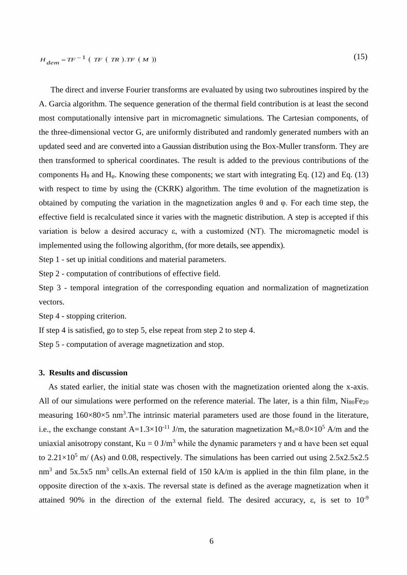
Let us now focus on the solution of Eq. (3) in the case of zero temperature. Fig. 1 shows the time

evolution of the average magnetization <Mx>.

It is worth noting that after applying the external field, the average magnetization, <Mx>,

remained constant and reached the reversal state for shorter periods of time for the thin film with

the small cell size as compared to the case with the large cell size. As a result, the speed of the

magnetization reversal process is increased when the cell size was reduced. The used integrating

scheme is characterized by an automatic selection and an updating of the time step. Therefore, it

leads during the computation of the reversal magnetization to a set of failed and successful steps to

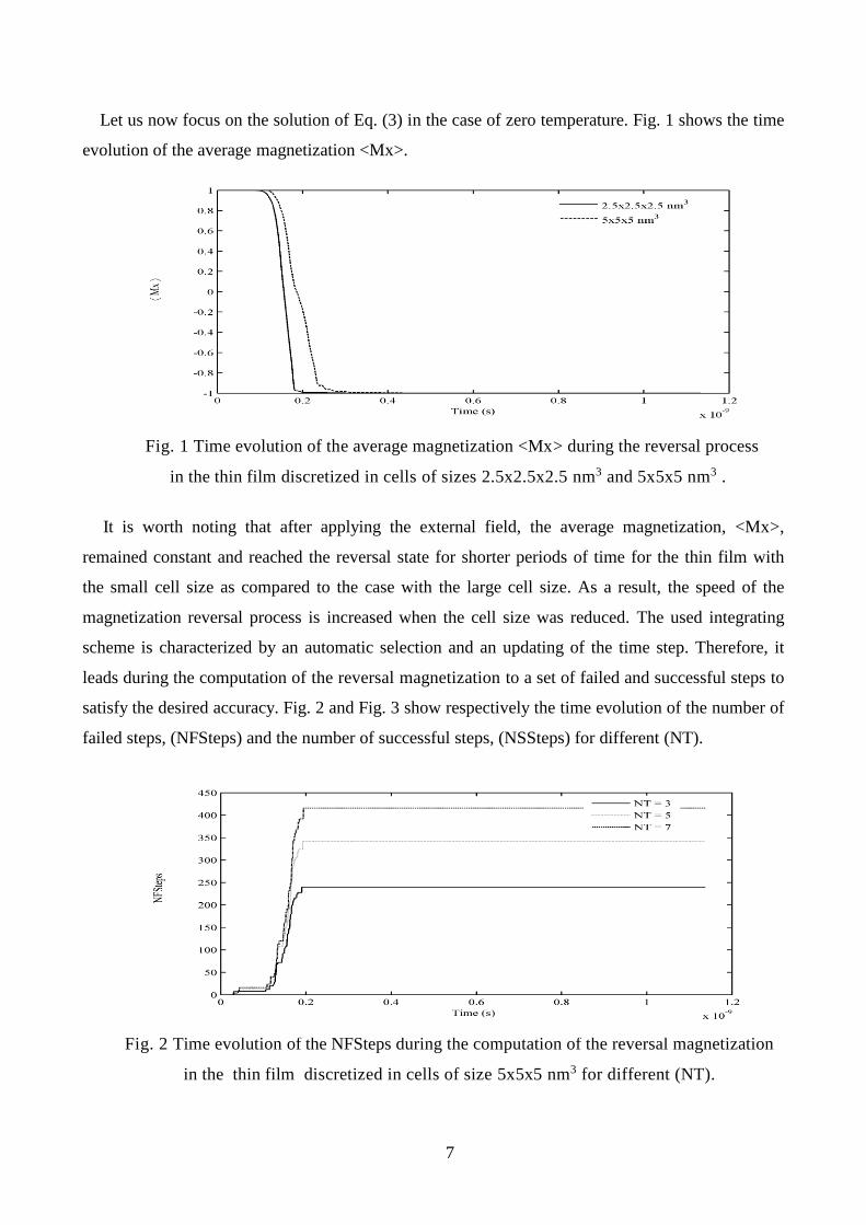
satisfy the desired accuracy. Fig. 2 and Fig. 3 show respectively the time evolution of the number of

failed steps, (NFSteps) and the number of successful steps, (NSSteps) for different (NT).

Fig. 1 Time evolution of the average magnetization <Mx> during the reversal process

in the thin film discretized in cells of sizes 2.5x2.5x2.5 nm3 and 5x5x5 nm3 .

Fig. 2 Time evolution of the NFSteps during the computation of the reversal magnetization

in the thin film discretized in cells of size 5x5x5 nm3 for different (NT).

8

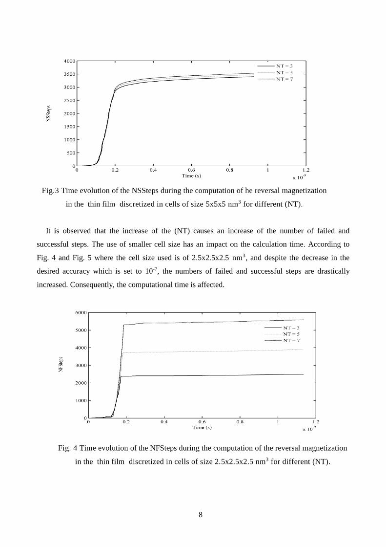
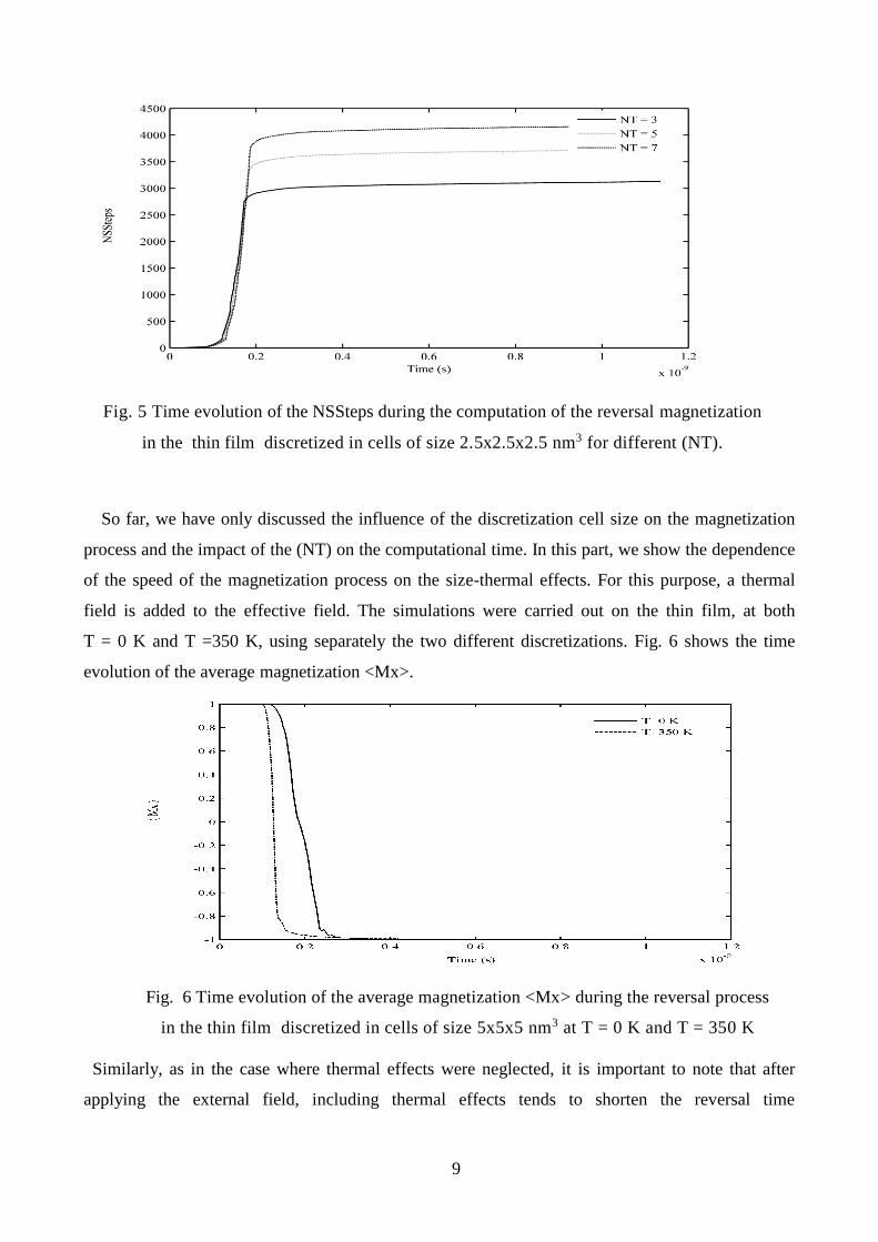
It is observed that the increase of the (NT) causes an increase of the number of failed and

successful steps. The use of smaller cell size has an impact on the calculation time. According to

Fig. 4 and Fig. 5 where the cell size used is of 2.5x2.5x2.5 nm3, and despite the decrease in the

desired accuracy which is set to 10-7, the numbers of failed and successful steps are drastically

increased. Consequently, the computational time is affected.

Fig.3 Time evolution of the NSSteps during the computation of he reversal magnetization

in the thin film discretized in cells of size 5x5x5 nm3 for different (NT).

Fig. 4 Time evolution of the NFSteps during the computation of the reversal magnetization

in the thin film discretized in cells of size 2.5x2.5x2.5 nm3 for different (NT).

9

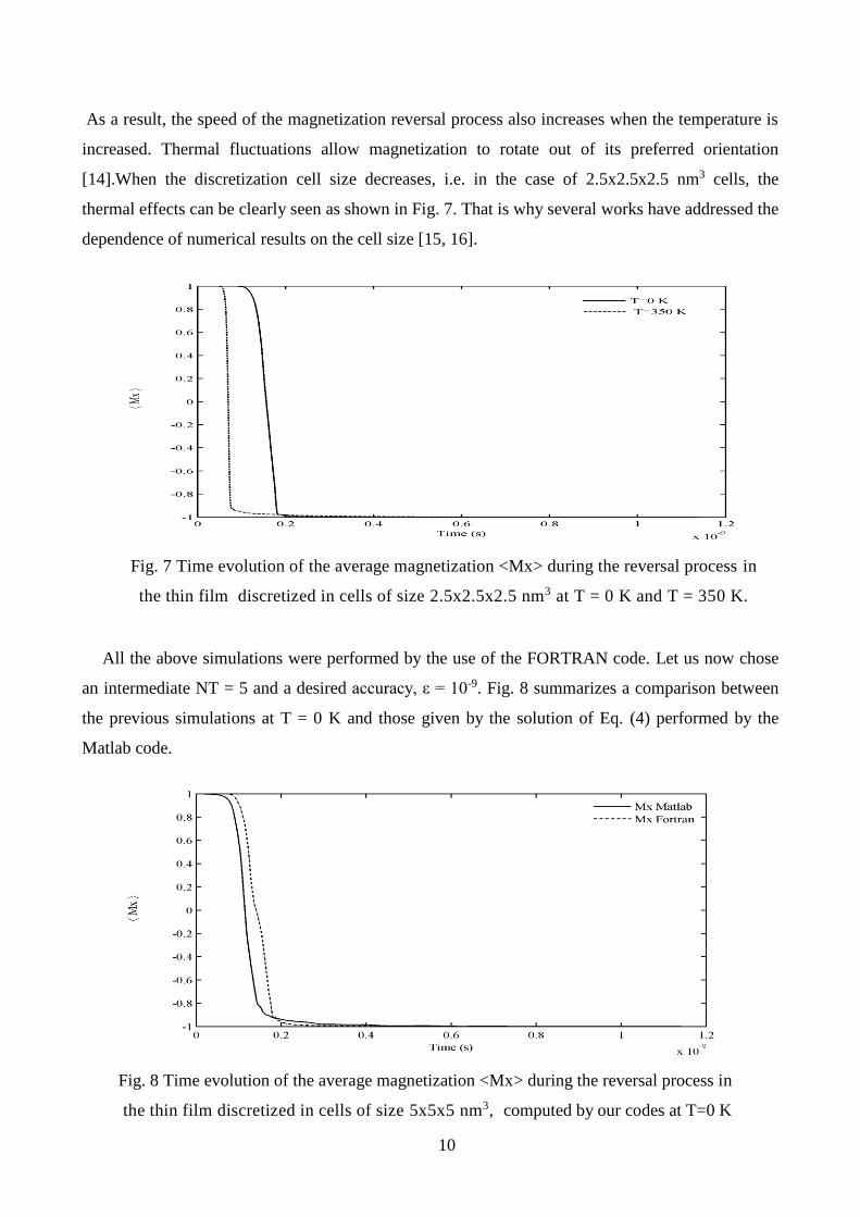
So far, we have only discussed the influence of the discretization cell size on the magnetization

process and the impact of the (NT) on the computational time. In this part, we show the dependence

of the speed of the magnetization process on the size-thermal effects. For this purpose, a thermal

field is added to the effective field. The simulations were carried out on the thin film, at both

T = 0 K and T =350 K, using separately the two different discretizations. Fig. 6 shows the time

evolution of the average magnetization <Mx>.

Similarly, as in the case where thermal effects were neglected, it is important to note that after

applying the external field, including thermal effects tends to shorten the reversal time

Fig. 6 Time evolution of the average magnetization <Mx> during the reversal process

in the thin film discretized in cells of size 5x5x5 nm3 at T = 0 K and T = 350 K

Fig. 5 Time evolution of the NSSteps during the computation of the reversal magnetization

in the thin film discretized in cells of size 2.5x2.5x2.5 nm3 for different (NT).

10

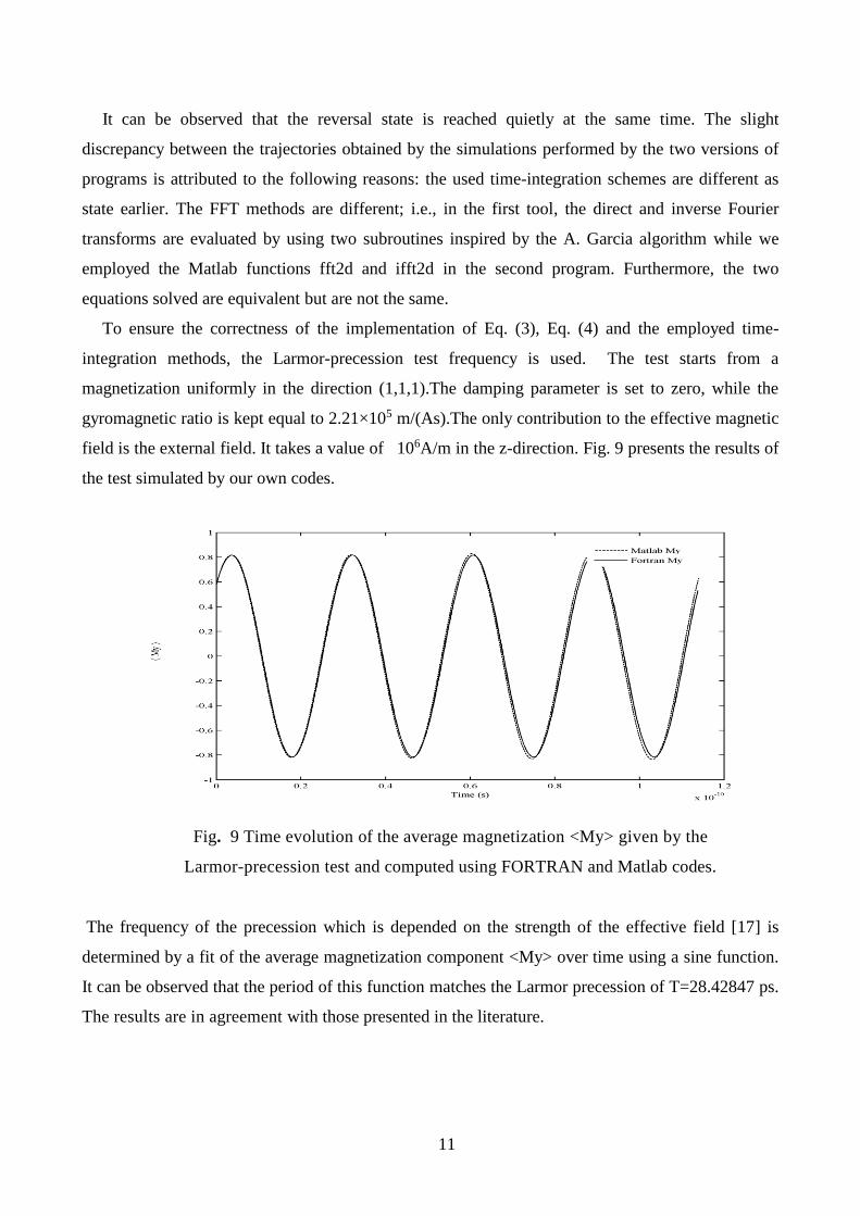
As a result, the speed of the magnetization reversal process also increases when the temperature is

increased. Thermal fluctuations allow magnetization to rotate out of its preferred orientation

[14].When the discretization cell size decreases, i.e. in the case of 2.5x2.5x2.5 nm3 cells, the

thermal effects can be clearly seen as shown in Fig. 7. That is why several works have addressed the

dependence of numerical results on the cell size [15, 16].

All the above simulations were performed by the use of the FORTRAN code. Let us now chose

an intermediate NT = 5 and a desired accuracy, ε = 10-9. Fig. 8 summarizes a comparison between

the previous simulations at T = 0 K and those given by the solution of Eq. (4) performed by the

Matlab code.

Fig. 8 Time evolution of the average magnetization <Mx> during the reversal process in

the thin film discretized in cells of size 5x5x5 nm3, computed by our codes at T=0 K

Fig. 7 Time evolution of the average magnetization <Mx> during the reversal process in

the thin film discretized in cells of size 2.5x2.5x2.5 nm3 at T = 0 K and T = 350 K.

11

It can be observed that the reversal state is reached quietly at the same time. The slight

discrepancy between the trajectories obtained by the simulations performed by the two versions of

programs is attributed to the following reasons: the used time-integration schemes are different as

state earlier. The FFT methods are different; i.e., in the first tool, the direct and inverse Fourier

transforms are evaluated by using two subroutines inspired by the A. Garcia algorithm while we

employed the Matlab functions fft2d and ifft2d in the second program. Furthermore, the two

equations solved are equivalent but are not the same.

To ensure the correctness of the implementation of Eq. (3), Eq. (4) and the employed time-

integration methods, the Larmor-precession test frequency is used. The test starts from a

magnetization uniformly in the direction (1,1,1).The damping parameter is set to zero, while the

gyromagnetic ratio is kept equal to 2.21×105 m/(As).The only contribution to the effective magnetic

field is the external field. It takes a value of 106A/m in the z-direction. Fig. 9 presents the results of

the test simulated by our own codes.

The frequency of the precession which is depended on the strength of the effective field [17] is

determined by a fit of the average magnetization component <My> over time using a sine function.

It can be observed that the period of this function matches the Larmor precession of T=28.42847 ps.

The results are in agreement with those presented in the literature.

Fig. 9 Time evolution of the average magnetization <My> given by the

Larmor-precession test and computed using FORTRAN and Matlab codes.

12

Conclusions

Two customized FORTRAN and Matlab codes have been developed based on solving both the

Gilbert and its equivalent equations. The magnetization reversal at zero and a finite temperature in a

permalloy thin film is analyzed using these tools. It is worth to note that the magnetization reversal

process is dependent on the cell size. The (NT) has an impact on the computational time at reduced

sizes. The slight discrepancy between the results obtained by the Matlab and the FORTRAN

programs is justified. A limited validation is carried out. Strong agreement is achieved between our

results and those presented in the literature. We would like to mention that a flexibility to extend

these tools and including others effects is allowed.

Acknowledgment

The authors warmly thank Mr. A. Bouchtob, lecturer at the University of Batna for his help and

assistance.

References

1. www.magnet.atp.tuwien.ac.at.sholtz/magpar,access date April 2010.

2. www.nmag.soton.ac.uk,access date January 2012.

3. www.math.nist.gov/oommf/,access date April 2014.

4. www.llgmicro.home.mindspring.com/, access date April 2015.

5. www.micromagus.de/,access date January 2016.

6. L.Neel,''Influence des fluctuations thermiques sur l'aimantation des grains

ferromagnétiques très fins'', Comptes rendus,vol. 228, pp. 664-666, 1949.

7. W. F. Brown,'' Thermal fluctuations of a single-domain particle'', Phys. Review, vol.130,

issue 5, pp. 1677-1686, 1963.

8. A. Romeo, G. Finocchio, M. Carpentieri, L.Torres, G. Consolo, B. Azzerboni, ''A numerical

solution of the magnetization reversal modeling in a permalloy thin film using a fifth order

Runge-Kutta method with adaptive step- size control'', Physica B. 403, pp. 464-468, 2008.

9. Novikov, E.A,''Runge kutta explicit methods: Algorithm of variable order and steps",

www.amse-modeling.org, access date February 2016.

10. www.garcia.org/nummeth/nummeth , access date June 2014.

11. H. Kronmüller, R. Hertal, ''Computational of magnetic structures and magnetization

processes in small particles'', J.Magn.Magn.Mat.vol.215-216, pp. 11-17, 2000.

12. M. Mansuripur, ''The physical principles of magneto- optical Recording'', Cambridge

university press, 1995.

13

13. Y. Nakatani, Y. Uesaka, N. Hayachi, ''Direct solution of the Landau-Lifshitz-Gilbert

equation for micromagnetics'', Japanese Journal of Applied Physics.vol 28,No.12 ,pp.

2485-2507, 1989.

14. V. Tsiantos, W. Scholz, D. suess, T. Schrefl , J. Fidler,'' The effect of the cell size in

langevin micromagnetic simulations '', J.Magn.Magn.Mat.vol.242-245, pp. 999-1001, 2002.

15. E. Matinez,L.Lopez-Diaz,L.Torres,C.J.Garcia-Cervera,"Minimizing cell size dependence in

Micromagnetics with thermal noise",J. Physics D:Appl. phys vol.40,No.4,pp.942-948,2007

16. J. Fidler,T. Shrefl,V.Tsiantos,W. Scholz,D.Suess, "Micromagnetic simulation of the

magnetic switching behavior of mesoscopic and nanoscopic structures",computational

materials science,vol.24,pp.163-174,2002

17. J. Stohr, H.C. Siegmann,"Magnetism from fundamentals to nanoscale dynamics",Springer-

Verlag, Berlin Heidelberg, 2006.

Appendix

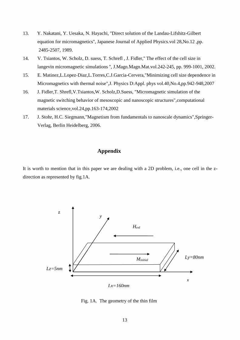
It is worth to mention that in this paper we are dealing with a 2D problem, i.e., one cell in the z-

direction as represented by fig.1A.

Minitial

Hext

z y

x

Lx=160nm

Fig. 1A. The geometry of the thin film

Lz=5nm

Ly=80nm

14

The magnetization in a computational cell, z,y,x is indexed by ,j,i in 2D and represented

in Cartesian coordinates by

zyx M,M,MM (1.A)

And in spherical coordinates by Eq.(9). The cell size is defined by

Nz/Lz

Ny/Ly

Nx/Lx

z

y

x

(2.A)

The change of the magnetization is caused by the total effective magnetic field

extdemanisexcheff HHHHH (3.A)

Where exchH , anisH , demH and extH are the standard contributions to the total effective field at zero

temperature. However, at a finite temperature the thermal field, thermH is added.

The demagnetizing field contribution is firstly obtained by calculation of the demagnetizing tensor

defined by the matrix, TR composed by nine demagnetizing coefficients.

zzzyzx

yzyyyx

xzxyxx

TRTRTR

TRTRTR

TRTRTR

TR (4.A)

These coefficients are evaluated using these formulas in the three dimensional case

x.Ir

yz.J.KgtanK,J,ITRxx

50

50501 1

1

0

1

0

1

0

(5.A)

rz.KlogTRK,J,ITR yxxy

501

1

0

1

0

1

0

(6.A)

Where

15

222222505050 z.Ky.Jx.Ir (7.A)

The other coefficients can be obtained by the simultaneous cyclic permutations of ,K,J,I

,, and z,y,x .

The computation of the demagnetizing tensor, TR is done using Cartesian coordinates in the case of

the use both the two codes.

In Matlab code

The Cartesian coordinates are used to express all the contributions of the effective field.

The contribution of the exchange field in a general three dimensional case is represented in

Cartesian coordinates by

22

1212

x

k,j,iMk,j,iMk,j,iM

M

AH xxx

s

x,exch

+

22

1212

y

k,j,iMk,j,iMk,j,iM

M

A yyy

s

(8.A)

+

22

1212

z

k,j,iMk,j,iMk,j,iM

M

A zzz

s

The other components of the exchange field are obtained by replacing x with y or z in the above

equation.

It is worth noting that the evaluation of the exchange field is enforced by the values of the boundary

conditions given by

0n

M

n

M

n

M zyx

(9.A)

Where n is the normal to the respective direction.

The contribution of the anisotropy field is defined by

16

MM

KH

s

uanis 2

0

2

(10.A)

The contribution of the external is uniform in each computational cell

The contribution of the demagnetizing field is computed using Eq. (15), where the functions

fft2d and ifft2d in Matlab are used respectively to compute (TF) and (TF-1).

Considering the reduced, form. Therefore, ss M

Mm,

M

Hh and

sMdtd , So

xh , yh and zh are the reduced components of the total effective field ,

xm , ym and zm are the reduced components of the magnetization.

The time integration of the three equations below is achieved using the standard Runge Kutta

method according to the simple algorithm presented in section.2.

zxxzzxyyxyyzzyx hmhmmhmhmmhmhm

d

dm

21

1 (11.A)

xyyxxyzzyzzxxz

yhmhmmhmhmmhmhm

d

dm

21

1 (12.A)

yzzyyxxzzxxyyxz hmhmmhmhmmhmhm

d

dm

21

1 (13.A)

In Fortran code

The spherical coordinates are used to express all the contributions of the effective field using

Eq.(10) and Eq.(11).

the components of the contribution of the anisotropic field

If the local axe of the anisotropy has an arbitrary direction, 0u specified by the angles 00 , and a

moment, M has a direction, ru specified by the angles , . Furthermore, the anisotropy energy

density is expressed as

2

01 u.uKe ruanis (14.A)

So, the components are expressed as

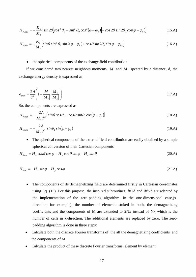
17

000

2

0

2

0

2 222 cossincoscossincossinM

KH

s

u

anis (15.A)

0000

2 22 sinsincossinsinsinM

KH

s

uanis (16.A)

the spherical components of the exchange field contribution

If we considered two nearest neighbors moments, M and 1M speared by a distance, d, the

exchange energy density is expressed as

Ss

exchM

M.

M

M

d

Ae 1

21

2 (17.A)

So, the components are expressed as

1112

2 cossincoscossin

dM

AH

s

exch (18.A)

112

2 sinsin

dM

AH

S

exch (19.A)

The spherical components of the external field contribution are easily obtained by a simple

spherical conversion of their Cartesian components

sinHsincosHcoscosHH zyxext (20.A)

cosHsinHH yxext (21.A)

The components of de demagnetizing field are determined firstly in Cartesian coordinates

using Eq. (15). For this purpose, the inspired subroutines, fft2d and ifft2d are adapted by

the implementation of the zero-padding algorithm. In the one-dimensional case,(x-

direction, for example), the number of elements stoked in both, the demagnetizing

coefficients and the components of M are extended to 2Nx instead of Nx which is the

number of cells in x-direction. The additional elements are replaced by zero. The zero-

padding algorithm is done in three steps:

Calculate both the discrete Fourier transforms of the all the demagnetizing coefficients and

the components of M

Calculate the product of these discrete Fourier transforms, element by element.

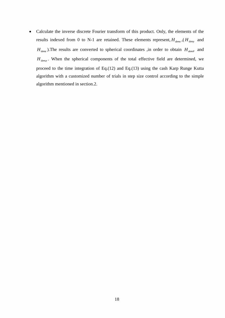
18

Calculate the inverse discrete Fourier transform of this product. Only, the elements of the

results indexed from 0 to N-1 are retained. These elements represent, demxH ,( demyH and

demzH ).The results are converted to spherical coordinates ,in order to obtain demH and

demH . When the spherical components of the total effective field are determined, we

proceed to the time integration of Eq.(12) and Eq.(13) using the cash Karp Runge Kutta

algorithm with a customized number of trials in step size control according to the simple

algorithm mentioned in section.2.