Embed Size (px)
Citation preview
International Journal of Management Studies ISSN(Print) 2249-0302 ISSN (Online)2231-2528 http://www.researchersworld.com/ijms/
Vol.–V, Issue –3(1), July 2018 [12]
DOI : 10.18843/ijms/v5i3(1)/03
DOIURL :http://dx.doi.org/10.18843/ijms/v5i3(1)/03
A single-vendor single-buyer supply chain coordination model with
price discount and benefit sharing in fuzzy environment
U. Sarkar,
Department of Mathematics,
MCKV Institute of Engineering, Liluah, Howrah, India
A. K. Jalan,
Department of Mathematics,
MCKV Institute of Engineering,
Liluah, Howrah, India
B.C. Giri,
Department of Mathematics,
Jadavpur University, Kolkata, India
ABSTRACT
Coordination among the participating members of a supply chain is a major issue for all
successful decision makers. In the literature, numerous supply chain models have been developed
based on exact (known) parameter-values. However, in reality, vagueness of parameter-values is
frequently observed in many circumstances. In this article, we develop a two-stage supply chain
model with a single vendor and a single buyer, and design a coordination mechanism through
price discount policy with incomplete information of demand and cost parameters. We first
develop the model imposing fuzziness in demand and then fuzziness in all the cost components. In
each case, centroid method is used for defuzzification. A solution procedure is outlined and
suitable numerical examples are given to determine the optimal results of the proposed fuzzy
models.
Keywords: supply chain management, coordination, price discount, fuzzy, centroid method.
INTRODUCTION:
The single-vendor single-buyer integrated production-inventory problem has received a maximum attention
from both academia and industry in recent years due to the growing focus on supply chain management.
Researchers have shown their keen interest on supply chain management realizing its potential to improve
performance of business firms at a reduced cost and delivery time. Moreover, an efficient management of
inventories across the entire supply chain through better coordination and cooperation can give better joint
benefit to all members involved. This leads the researchers to develop the strategic coordination between vendor
and buyer of a supply chain.
One of the first works dealing with integrated vendor-buyer supply chain is due to Goyal (1976). In his work, he
addressed a simple supply chain model with single supplier and single customer problem. Later, Banerjee
(1988) developed a joint economic lot size model assuming that the vendor manufactures at a finite rate. He
considered a lot-for-lot model where the vendor produces each buyer shipment as a separate batch. Goyal
(1988) argued this assumption and proposed that producing a batch which is made up of equal shipments
provides lower cost. Lu (1995) developed a single vendor single buyer model with equal shipments and derived
its optimal solutions. In another work, Goyal (1995) showed that different shipment size policy could produce a
better solution. He considered successive shipments within a production batch increased by a constant factor
which is equal to the ratio of production rate over the demand rate. Hill (1999) proposed a globally optimal
batching and shipping policy for single vendor single buyer supply chain. Considering unequal and equal
shipments from the vendor to the buyer, Hogue and Goyal (2000) derived a solution procedure for optimal
International Journal of Management Studies ISSN(Print) 2249-0302 ISSN (Online)2231-2528 http://www.researchersworld.com/ijms/
Vol.–V, Issue –3(1), July 2018 [13]
production quantity. They considered capacity constraint of the transport equipment in their model. Ben-Daya
and Hariga (2004) used stochastic demand and variable lead time in their model and showed that coordination is
effective from the vendor’s as well as the buyer’s perspectives. Considering probabilistic demand and using
quantity discount policy, Li and Liu (2006) proposed a model to achieve coordination between the vendor and
the buyer. Qin et al. (2007) developed a single vendor single buyer integrated inventory model considering
volume discount, franchise fees and price sensitive demand. Sajadieh et al. (2009) proposed another single
vendor single buyer supply chain model in which the vendor delivers the production batch to the buyer in 𝑛
equal shipments and the lead time is stochastic. Yang (2010) contributed, in his supply chain model, on the
present value analysis assuming variable lead time. Masihabadi and Eshghi (2011) developed a model for
coordinating seller-buyer with a proper allocation of chain’s surplus profit assuming a general side payment
contract. Shahrjerdi et al. (2011) proposed a cooperative and non-cooperative seller-buyer supply chain model
and derived the optimal decisions. Saha et al. (2012) studied a supply chain model considering stock and price
dependent selling rates in the declining market. Moharana et al. (2012) developed a supply chain model where
they investigated on the stability of coordination, collaboration and integration between the buyer and the
vendor. Shah et al. (2013) proposed a single-supplier single-buyer inventory system to derive the optimal
pricing, shipments and ordering policies. They assumed the demand as price-sensitive and stock dependent and
also the order-linked trade-credit. Dey and Giri (2014) proposed a vendor-buyer model under imperfect
production; Zhang et al. (2016) considered discount policy to develop their model; Li et al. (2017) investigated
the environmental impacts in their model.
In the above studies, researchers used crisp values for the cost parameters. However, in reality, these costs may
not be known as fixed quantities. For example, set up cost and holding cost of the vendor may vary due to some
changes in environment. A retailer may face the same problem to determine the replenishment cost. A lot of
probabilistic models have been developed to capture various uncertainties in reality. Researchers have used
statistical methods to estimate the parameter(s) of probability distribution from the past data. However, past
data may not be always available or reliable. To cope with this problem, one can use possibility theory rather
than probability theory and represent uncertainty by possibility distribution.
Zadeh (1965) was first to introduce fuzzy set theory to handle these vague situations. In recent years, the theory
of fuzzy sets and fuzzy logic has found wide applications in the field of operations management. Yao and Lee
(1996) proposed a back order fuzzy inventory model with fuzzy order quantity as triangular and trapezoidal
fuzzy numbers and shortage cost as a crisp parameter. Yao and Chiang (2003), in their inventory model without
backorder, fuzzified the total demand and cost of storing by triangular fuzzy numbers and defuzzified the total
cost by centroid and signed distance methods. Chiang et al. (2005) represented the storing cost, backorder cost,
ordering cost, total demand, order quantity and shortage quantity by triangular fuzzy numbers and defuzzified
by signed distance method. Tutunchu and Akoz (2008) used fuzzy setup cost, holding cost and shortage cost,
and defuzzified by Park’s Median Rule. Lin (2008) fuzzified the expected demand, shortage and backorder rate
and used signed distance method to defuzzify the cost function obtained in the fuzzy sense. Sadi-Nezhad et al.
(2011) in their continuous review inventory model fuzzified the setup cost, holding cost and shortage cost and
defuzzified by signed distance and possibilistic mean value methods. Lee and Lin (2011), Sarkar and
Chakrabarti (2012), Mahapatra et al. (2012) proposed some fuzzy inventory models.
The literature shows that there has been a significant development of inventory models under uncertainty using
the concept of fuzzy sets. However, study of supply chain model in fuzzy environment is limited. Mahata et al.
(2005) proposed a joint economic lot size model for both buyer and vendor assuming the order quantity as a
fuzzy variable and other parameters as deterministic. Corbett and Groote (2000) developed a supply chain
model under asymmetric information where they considered quantity discount policy. Petrovic et al. (1999)
used fuzzy set theory in their supply chain model. Gunasekaran et al. (2006) contributed in optimizing the order
quantity with fuzzy approach. Eric Sucky (2006) proposed a two-staged supply chain coordination problem
under asymmetric information where the assumption is that the buyers have two sets of predefined
(deterministic) cost structures and the vendor does not know in which particular cluster a particular buyer
belongs. However, this model has a limitation to address a wide range of cost structures that a buyer can
possibly have. Ganga and Carpinetti (2011) and Costantino et al. (2012) proposed some valuable supply chain
models in fuzzy environment. Sinha and Sarmah (2008) extended their work considering quantity discount
policy. They assumed ordering cost, inventory holding cost of the buyer and demand as fuzzy variables.
Taleizadeh et al. (2013) considered fuzzy-lead times and suggested two hybrid procedures to solve the
integrated inventory problems. Mahata (2015) developed a single-vendor single-buyer model with fuzzy order
quantity and fuzzy shortage quantity. Priyam and Uthayakumar (2016) proposed a fuzzy model under variable
International Journal of Management Studies ISSN(Print) 2249-0302 ISSN (Online)2231-2528 http://www.researchersworld.com/ijms/
Vol.–V, Issue –3(1), July 2018 [14]
lead time and service level constraint. Jauhari and Saga (2017) considered set up cost reduction and service
level constraint in their vendor-buyer model.
In this article, we consider the demand at the buyer and all the cost components of the vendor and buyer as
fuzzy variables. We use centroid method for defuzzification of the average fuzzy cost. The rest of the paper is
organized as follows: In Section 2, some assumptions and notations are given. In Section 3, the mathematical
formulation of the model is given. Section 4 expresses some preliminaries on fuzzy set theory and
defuzzification method. Section 5 deals with the implementation of fuzzy concept in the inventory system.
Numerical examples are given in Section 6 to illustrate the developed models and perform sensitivity analysis
with respect to some model-parameters. Finally, we conclude the paper in Section 7.
ASSUMPTIONS AND NOTATIONS:
The following assumptions are made for developing the proposed model:
(i) A single-type of product is considered.
(ii) The supply chain consists of a single buyer and a single vendor.
(iii) The vendor’s production rate is finite and is greater than the buyer’s demand rate.
(iv) The vendor offers price discount to the buyer.
(v) Each production lot size of the vendor is transported to buyer in 𝑛 equal shipments.
(vi) The vendor’s production process is reliable (perfect).
(vii) Shortages are not allowed in buyer’s inventory.
The following notations are used to construct our mathematical model:
𝐷 (��) : Demand rate in units per unit time in crisp (fuzzy). 1
𝑝 : Production rate in units per unit time.
𝑛 : Number of shipments from the vendor to the buyer.
𝑄 : Size of equal shipments from the vendor to the buyer.
𝐶0 (��𝑜) : Vendor’s set up cost in crisp (fuzzy).
𝐶1 (��1) : Buyer’s ordering cost for each order of size 𝑛𝑄 in crisp (fuzzy).
𝐶2 (��2) : Buyer’s transportation cost for each shipment of size 𝑄 in crisp (fuzzy).
𝐶3 (��3) : Vendor’s unit production cost in crisp (fuzzy).
𝐶0 (��𝑜) : Vendor’s undiscounted sale price in crisp (fuzzy).
𝐶5 : Vendor’s discounted sale price in crisp.
𝐶6 (��6) : Buyer’s unit sale price in crisp.
ℎ𝑏 (ℎ𝑏) : Buyer’s holding cost per unit per time in crisp (fuzzy).
ℎ𝑣 (ℎ𝑣) : Vendor’s holding cost per unit per time for the vendor in crisp (fuzzy).
𝜆 : Level of benefit offered by the vendor to the buyer.
MATHEMATICAL FORMULATION:
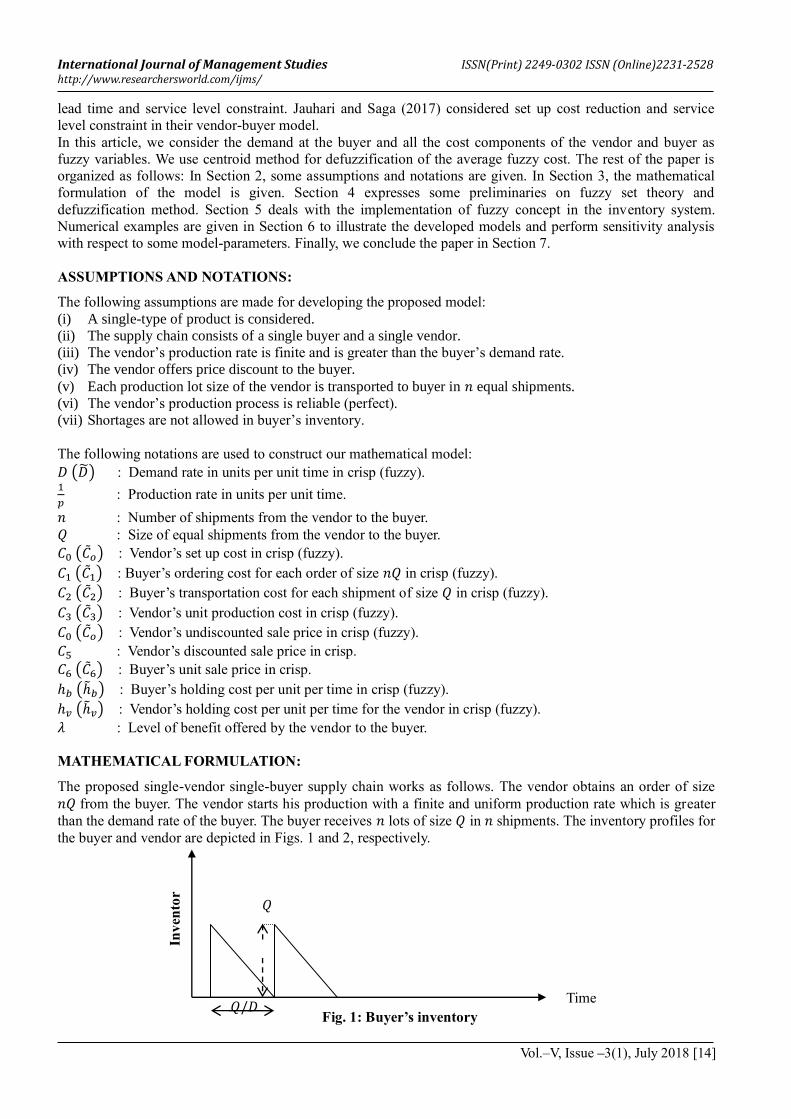
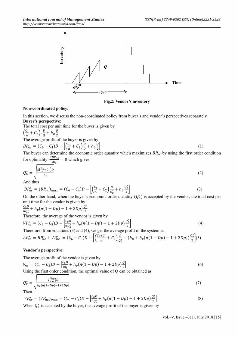
The proposed single-vendor single-buyer supply chain works as follows. The vendor obtains an order of size
𝑛𝑄 from the buyer. The vendor starts his production with a finite and uniform production rate which is greater
than the demand rate of the buyer. The buyer receives 𝑛 lots of size 𝑄 in 𝑛 shipments. The inventory profiles for
the buyer and vendor are depicted in Figs. 1 and 2, respectively.
𝑄/𝐷
𝑄
Time
Inv
ento
r
y
Fig. 1: Buyer’s inventory
International Journal of Management Studies ISSN(Print) 2249-0302 ISSN (Online)2231-2528 http://www.researchersworld.com/ijms/
Vol.–V, Issue –3(1), July 2018 [15]
Non-coordinated policy:
In this section, we discuss the non-coordinated policy from buyer’s and vendor’s perspectives separately.
Buyer’s perspective:
The total cost per unit time for the buyer is given by
.𝐶1
𝑛+ 𝐶2/ .
𝐷
𝑄+ ℎ𝑏
𝑄
2
The average profit of the buyer is given by
𝐵𝑃𝑛𝑐 = (𝐶6 − 𝐶4)𝐷 − 0.𝐶1
𝑛+ 𝐶2/
𝐷
𝑄+ ℎ𝑏
𝑄
21 (1)
The buyer can determine the economic order quantity which maximizes 𝐵𝑃𝑛𝑐 by using the first order condition
for optimality 𝑑𝐵𝑃𝑛𝑐
𝑑𝑄= 0 which gives
𝑄𝑏∗ = √
2.𝐶1𝑛:𝐶2/𝐷
ℎ𝑏 (2)
And thus
𝐵𝑃𝑛𝑐∗ = (𝐵𝑃𝑛𝑐)𝑚𝑎𝑥 = (𝐶6 − 𝐶4)𝐷 − [.
𝐶1
𝑛+ 𝐶2/
𝐷
𝑄𝑏∗ + ℎ𝑏
𝑄𝑏∗
2] (3)
On the other hand, when the buyer’s economic order quantity (𝑄𝑏∗) is accepted by the vendor, the total cost per
unit time for the vendor is given by 𝐶0𝐷
𝑛𝑄𝑏∗ + ℎ𝑣*𝑛(1 − 𝐷𝑝) − 1 + 2𝐷𝑝+
𝑄𝑏∗
2
Therefore, the average of the vendor is given by
𝑉𝑃𝑛𝑐∗ = (𝐶4 − 𝐶3)𝐷 − [
𝐶0𝐷
𝑛𝑄𝑏∗ + ℎ𝑣*𝑛(1 − 𝐷𝑝) − 1 + 2𝐷𝑝+
𝑄𝑏∗
2] (4)
Therefore, from equations (3) and (4), we get the average profit of the system as
𝐴𝑃𝑛𝑐∗ = 𝐵𝑃𝑛𝑐
∗ + 𝑉𝑃𝑛𝑐∗ = (𝐶6 − 𝐶3)𝐷 − [.
𝐶0:𝐶1
𝑛+ 𝐶2/
𝐷
𝑄𝑏∗ + (ℎ𝑏 + ℎ𝑣*𝑛(1 − 𝐷𝑝) − 1 + 2𝐷𝑝+)
𝑄𝑏∗
2](5)
Vendor’s perspective:
The average profit of the vendor is given by
𝑉𝑛𝑐 = (𝐶4 − 𝐶3)𝐷 − 0𝐶0𝐷
𝑛𝑄+ ℎ𝑣*𝑛(1 − 𝐷𝑝) − 1 + 2𝐷𝑝+
𝑄
21 (6)
Using the first order condition, the optimal value of Q can be obtained as
𝑄𝑣∗ = √
2.𝐶0𝑛/𝐷
ℎ𝑣*𝑛(1;𝐷𝑝);1:2𝐷𝑝+ (7)
Then
𝑉𝑃𝑛𝑐∗ = (𝑉𝑃𝑛𝑐)𝑚𝑎𝑥 = (𝐶4 − 𝐶3)𝐷 − 0
𝐶0𝐷
𝑛𝑄𝑣∗ + ℎ𝑣*𝑛(1 − 𝐷𝑝) − 1 + 2𝐷𝑝+
𝑄𝑣∗
21 (8)
When 𝑄𝑣∗ is accepted by the buyer, the average profit of the buyer is given by
Fig.2: Vendor’s inventory
Time
Inven
tory
𝑛𝑄/𝐷
𝑸
𝑸/𝑫
International Journal of Management Studies ISSN(Print) 2249-0302 ISSN (Online)2231-2528 http://www.researchersworld.com/ijms/
Vol.–V, Issue –3(1), July 2018 [16]
𝐵𝑃𝑛𝑐∗ = (𝐶6 − 𝐶4)𝐷 − 0.
𝐶1
𝑛+ 𝐶2/
𝐷
𝑄𝑣∗ + ℎ𝑏
𝑄𝑣∗
21 (9)
Therefore, from equations (8) and (9), we get the average profit of the system as
𝐴𝑃𝑛𝑐∗ = 𝑉𝑃𝑛𝑐
∗ + 𝐵𝑃𝑛𝑐∗ = (𝐶6 − 𝐶3)𝐷 − 0.
𝐶0:𝐶1
𝑛+ 𝐶2/
𝐷
𝑄𝑣∗ + (ℎ𝑏 + ℎ𝑣*𝑛(1 − 𝐷𝑝) − 1 + 2𝐷𝑝+)
𝑄𝑣∗
21(10)
Coordinated policy:
When the vendor’s discounted sale price is 𝐶5 per unit then the average profit of the buyer is given by
𝐵𝑃𝑐 = (𝐶6 − 𝐶5)𝐷 − 0.𝐶1
𝑛+ 𝐶2/
𝐷
𝑄+ ℎ𝑏
𝑄
21 (11)
The average profit of the vendor is given by
𝑉𝑃𝑐 = (𝐶5 − 𝐶3)𝐷 − 0𝐶0𝐷
𝑛𝑄+ ℎ𝑣*𝑛(1 − 𝐷𝑝) − 1 + 2𝐷𝑝+
𝑄
21 (12)
From equations (11) and (12), the average co-ordinated profit of the supply chain is given by
𝐴𝑃𝑐 = 𝐵𝑃𝑐 + 𝑉𝑃𝑐 = (𝐶6 − 𝐶3)𝐷 − 0.𝐶0:𝐶1
𝑛+ 𝐶2/
𝐷
𝑄+ (ℎ𝑏 + ℎ𝑣*𝑛(1 − 𝐷𝑝) − 1 + 2𝐷𝑝+)
𝑄
21 (13)
Our objective is to determine the optimal number of shipments n* and the shipment size Q
* so that the average
co-ordination profit 𝐴𝑃𝑐 is maximized. The first order optimality condition 𝑑𝐴𝑃𝑐
𝑑𝑄= 0 gives
𝑄∗ = √2.
𝐶0+𝐶1𝑛
:𝐶2/𝐷
ℎ𝑏:ℎ𝑣*𝑛(1;𝐷𝑝);1:2𝐷𝑝+ (14)
Now, benefit of the buyer if price discount is implemented, is given by
𝐵𝑃𝑏 = (𝐵𝑃𝑐 − 𝐵𝑃𝑛𝑐∗ ) = {
(𝐶4 − 𝐶5)𝐷 + .𝐶1
𝑛+ 𝐶2/ (
1
𝑄𝑏∗ −
1
𝑄∗)𝐷 +
ℎ𝑏
2(𝑄𝑏
∗ − 𝑄∗)
(𝐶4 − 𝐶5)𝐷 + .𝐶1
𝑛+ 𝐶2/ .
1
𝑄𝑣∗ −
1
𝑄∗/𝐷 +
ℎ𝑏
2(𝑄𝑣
∗ − 𝑄∗) (15.a)
and benefit of the vendor is given by
𝐵𝑃𝑣 = (𝑉𝑃𝑐 − 𝑉𝑃𝑛𝑐∗ ) = {
(𝐶5 − 𝐶4)𝐷 +𝐶0𝐷
𝑛(1
𝑄𝑏∗ −
1
𝑄∗) +
ℎ𝑣
2(𝑄𝑏
∗ − 𝑄∗)*𝑛(1 − 𝐷𝑝) − 1 + 2𝐷𝑝+
(𝐶5 − 𝐶4)𝐷 +𝐶0𝐷
𝑛.1
𝑄𝑣∗ −
1
𝑄∗/ +
ℎ𝑣
2(𝑄𝑣
∗ − 𝑄∗)*𝑛(1 − 𝐷𝑝) − 1 + 2𝐷𝑝+ (15.b)
It is assumed that the vendor offers the buyer a certain level of co-ordination benefit such that
𝐵𝑃𝑏 = 𝜆𝐵𝑃𝑣 , 𝜆 ≥ 0 (15.c)
Therefore, from equations (15.a), (15.b) and (15.c), we get
𝐶5 =
{
𝐶4 +
(1
𝑄𝑏∗;
1
𝑄∗)
(1:𝜆).𝐶1;𝜆𝐶0
𝑛+ 𝐶2/ +
(𝑄𝑏∗;𝑄∗)
2𝐷(1:𝜆),ℎ𝑏 − 𝜆ℎ𝑣*𝑛(1 − 𝐷𝑝) − 1 + 2𝐷𝑝+-
𝐶4 +(1
𝑄𝑣∗;
1
𝑄∗)
(1:𝜆).𝐶1;𝜆𝐶0
𝑛+ 𝐶2/ +
(𝑄𝑣∗;𝑄∗)
2𝐷(1:𝜆),ℎ𝑏 − 𝜆ℎ𝑣*𝑛(1 − 𝐷𝑝) − 1 + 2𝐷𝑝+-
(16)
Theorem 1: The average joint profit 𝐴𝑃𝑐 is concave with respect to 𝑄.
Proof: We have from (13),
𝐴𝑃𝑐 = (𝐶6 − 𝐶3)𝐷 − 0.𝐶0:𝐶1
𝑛+ 𝐶2/
𝐷
𝑄+ (ℎ𝑏 + ℎ𝑣*𝑛(1 − 𝐷𝑝) − 1 + 2𝐷𝑝+)
𝑄
21
Therefore, 𝑑𝐴𝑃𝑐
𝑑𝑄= .
𝐶0:𝐶1
𝑛+ 𝐶2/
𝐷
𝑄2− (ℎ𝑏 + ℎ𝑣*𝑛(1 − 𝐷𝑝) − 1 + 2𝐷𝑝+)
1
2
and 𝑑2𝐴𝑃𝑇𝑐
𝑑𝑄2= −2.
𝐶0:𝐶1
𝑛+ 𝐶2/
𝐷
𝑄3
Since 𝐶0 > 0, 𝐶1 > 0, 𝐶2 > 0, 𝐷 > 0, 𝑛 > 0 and 𝑄 > 0, we get 𝑑2𝐴𝑃𝑐
𝑑𝑄2< 0.
Thus the average joint profit 𝐴𝑃𝑐 is a concave function in 𝑄.
FUZZY PRELIMINARIES:
In this section, the necessary background and some notions of fuzzy set theory are given.
Definition 1:
Let 𝑋 denote a universal set. Then the fuzzy subset �� of 𝑋 is defined by its membership function 𝜇��(𝑥): 𝑋 →
International Journal of Management Studies ISSN(Print) 2249-0302 ISSN (Online)2231-2528 http://www.researchersworld.com/ijms/
Vol.–V, Issue –3(1), July 2018 [17]
,0,1- which assigns a real number 𝜇��(𝑥) in the interval ,0, 1- to each element 𝑥𝜖𝑋 and 𝜇��(𝑥) shows the grade
of membership of 𝑥𝜖��.
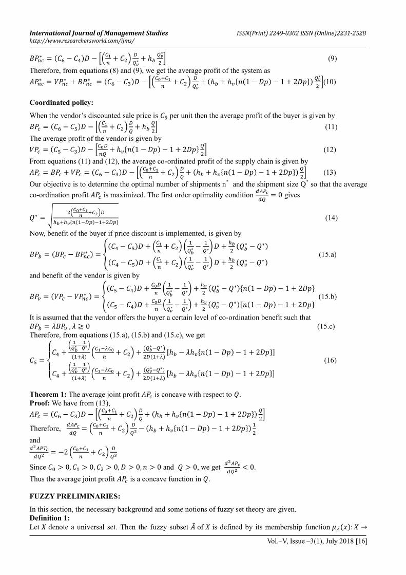
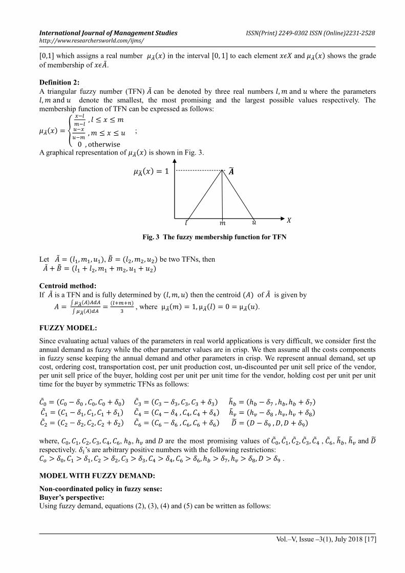
Definition 2:
A triangular fuzzy number (TFN) �� can be denoted by three real numbers 𝑙, 𝑚 and 𝑢 where the parameters
𝑙, 𝑚 and 𝑢 denote the smallest, the most promising and the largest possible values respectively. The
membership function of TFN can be expressed as follows:
𝜇��(𝑥) = {
𝑥;𝑙
𝑚;𝑙 , 𝑙 ≤ 𝑥 ≤ 𝑚
𝑢;𝑥
𝑢;𝑚 , 𝑚 ≤ 𝑥 ≤ 𝑢
0 , otherwise
;
A graphical representation of 𝜇��(𝑥) is shown in Fig. 3.
Let �� = (𝑙1, 𝑚1, 𝑢1), �� = (𝑙2, 𝑚2, 𝑢2) be two TFNs, then
�� + �� = (𝑙1 + 𝑙2, 𝑚1 +𝑚2, 𝑢1 + 𝑢2)
Centroid method:
If �� is a TFN and is fully determined by (𝑙,𝑚, 𝑢) then the centroid (𝐴) of �� is given by
𝐴 = ∫𝜇��(𝐴)𝐴𝑑𝐴
∫𝜇��(𝐴)𝑑𝐴=
(𝑙:𝑚:𝑛)
3 , where μ��(𝑚) = 1, μ��(𝑙) = 0 = μ��(𝑢).
FUZZY MODEL:
Since evaluating actual values of the parameters in real world applications is very difficult, we consider first the
annual demand as fuzzy while the other parameter values are in crisp. We then assume all the costs components
in fuzzy sense keeping the annual demand and other parameters in crisp. We represent annual demand, set up
cost, ordering cost, transportation cost, per unit production cost, un-discounted per unit sell price of the vendor,
per unit sell price of the buyer, holding cost per unit per unit time for the vendor, holding cost per unit per unit
time for the buyer by symmetric TFNs as follows:
��0 = (𝐶0 − 𝛿0 , 𝐶0, 𝐶0 + 𝛿0)
��1 = (𝐶1 − 𝛿1, 𝐶1, 𝐶1 + 𝛿1)
��2 = (𝐶2 − 𝛿2, 𝐶2, 𝐶2 + 𝛿2)
��3 = (𝐶3 − 𝛿3, 𝐶3, 𝐶3 + 𝛿3)
��4 = (𝐶4 − 𝛿4 , 𝐶4, 𝐶4 + 𝛿4)
��6 = (𝐶6 − 𝛿6 , 𝐶6, 𝐶6 + 𝛿6)
ℎ𝑏 = (ℎ𝑏 − 𝛿7 , ℎ𝑏, ℎ𝑏 + 𝛿7)
ℎ𝑣 = (ℎ𝑣 − 𝛿8 , ℎ𝑣 , ℎ𝑣 + 𝛿8)
�� = (𝐷 − 𝛿9 , 𝐷, 𝐷 + 𝛿9)
where, 𝐶0, 𝐶1, 𝐶2, 𝐶3, 𝐶4, 𝐶6, ℎ𝑏, ℎ𝑣 and 𝐷 are the most promising values of ��0, ��1, ��2, ��3, ��4 , ��6, ℎ𝑏, ℎ𝑣 and ��
respectively. 𝛿𝑖’s are arbitrary positive numbers with the following restrictions:
𝐶𝑜 > 𝛿0, 𝐶1 > 𝛿1, 𝐶2 > 𝛿2, 𝐶3 > 𝛿3, 𝐶4 > 𝛿4, 𝐶6 > 𝛿6, ℎ𝑏 > 𝛿7, ℎ𝑣 > 𝛿8, 𝐷 > 𝛿9 .
MODEL WITH FUZZY DEMAND:
Non-coordinated policy in fuzzy sense:
Buyer’s perspective:
Using fuzzy demand, equations (2), (3), (4) and (5) can be written as follows:
𝜇A(𝑥) = 1 ---------------------
𝑙 𝑚 𝑢 𝑋
Fig. 3 The fuzzy membership function for TFN
��
International Journal of Management Studies ISSN(Print) 2249-0302 ISSN (Online)2231-2528 http://www.researchersworld.com/ijms/
Vol.–V, Issue –3(1), July 2018 [18]
��𝑏∗ = √
2.𝐶1𝑛:𝐶2/��
ℎ𝑏 (17.a)
𝐵��𝑛𝑐∗ = (𝐶6 − 𝐶4)�� − [.
𝐶1
𝑛+ 𝐶2/
��
��𝑏∗ + ℎ𝑏
��𝑏∗
2] (17.b)
𝑉��𝑛𝑐∗ = (𝐶4 − 𝐶3)�� − [
𝐶0��
𝑛��𝑏∗ + ℎ𝑣{𝑛(1 − ��𝑝) − 1 + 2��𝑝}
��𝑏∗
2] (17.c)
𝐴��𝑛𝑐∗ = (𝐶6 − 𝐶3)�� − [.
𝐶0:𝐶1
𝑛+ 𝐶2/
��
��𝑏∗ + ( ℎ𝑏 + ℎ𝑣{𝑛(1 − ��𝑝) − 1 + 2��𝑝})
��𝑏∗
2] (17.d)
Vendor’s perspective:
After imposing fuzziness on demand equations (7), (8), (9) and (10) give
��𝑣∗ = √
2.𝐶0𝑛/��
ℎ𝑣*𝑛(1;𝐷𝑝);1:2𝐷𝑝+ (18.a)
𝑉��𝑛𝑐∗ = (𝐶4 − 𝐶3)�� − 0
𝐶0��
𝑛��𝑣∗ + ℎ𝑣{𝑛(1 − ��𝑝) − 1 + 2��𝑝}
��𝑣∗
21 (18.b)
𝐵��𝑛𝑐∗ = (𝐶6 − 𝐶4)�� − 0.
𝐶1
𝑛+ 𝐶2/
��
��𝑣∗ + ℎ𝑏
��𝑣∗
21 (18.c)
𝐴��𝑛𝑐∗ = (𝐶6 − 𝐶3)�� − 0.
𝐶0:𝐶1
𝑛+ 𝐶2/
��
��𝑣∗ + ( ℎ𝑏 + ℎ𝑣{𝑛(1 − ��𝑝) − 1 + 2��𝑝})
��𝑣∗
21 (18.d)
Coordinated policy in fuzzy sense:
In fuzzy demand sense, equations (14), (11), (12), (13) and (16) take the forms as:
��∗ = √2.
𝐶0+𝐶1𝑛
:𝐶2/��
ℎ𝑏:ℎ𝑣*𝑛(1;��𝑝);1:2��𝑝+ (19.a)
��5∗ =
{
𝐶4 +
(1
��𝑏∗;
1
𝑄∗)
(1:𝜆).𝐶1;𝜆𝐶0
𝑛+ 𝐶2/ +
(��𝑏∗;𝑄∗)
2��(1:𝜆)[ℎ𝑏 − 𝜆ℎ𝑣{𝑛(1 − ��𝑝) − 1 + 2��𝑝}]
𝐶4 +(1
��𝑣∗;
1
𝑄∗)
(1:𝜆).𝐶1;𝜆𝐶0
𝑛+ 𝐶2/ +
(��𝑣∗;𝑄∗)
2��(1:𝜆)[ℎ𝑏 − 𝜆ℎ𝑣{𝑛(1 − ��𝑝) − 1 + 2��𝑝}]
(19.b)
𝐵��𝑐∗ = (𝐶6 − 𝐶5)�� − 0.
𝐶1
𝑛+ 𝐶2/
��
𝑄+ ℎ𝑏
𝑄
21 (19.c)
𝑉��𝑐∗ = (𝐶5 − 𝐶3)𝐷 − 0
𝐶0��
𝑛𝑄+ ℎ𝑣{𝑛(1 − ��𝑝) − 1 + 2��𝑝}
𝑄
21 (19.d)
𝐴��𝑐∗ = (𝐶6 − 𝐶3)�� − 0.
𝐶0:𝐶1
𝑛+ 𝐶2/
��
��∗+ ( ℎ𝑏 + ℎ𝑣{𝑛(1 − ��𝑝) − 1 + 2��𝑝})
��∗
21 (19.e)
MODEL WITH FUZZY COST COMPONENTS:
Non-coordinated policy in fuzzy sense:
Buyer’s perspective:
Using fuzzy costs, equations (2), (3), (4) and (5) become
��𝑏∗ = √
2(��1𝑛:��2)𝐷
ℎ𝑏 (20.a)
𝐵��𝑛𝑐∗ = (��6 − ��4)𝐷 − [.
��1
𝑛+ ��2/
𝐷
��𝑏∗ + ℎ𝑏
��𝑏∗
2] (20.b)
𝑉��𝑛𝑐∗ = (��4 − ��3)𝐷 − [
��𝑜𝐷
𝑛��𝑏∗ + ℎ𝑣*𝑛(1 − 𝐷𝑝) − 1 + 2𝐷𝑝+
��𝑏∗
2] (20.c)
𝐴��𝑛𝑐∗ = (��6 − ��3)𝐷 − [.
��𝑜:��1
𝑛+ ��2/
𝐷
��𝑏∗ + ( ℎ𝑏 + ℎ𝑣*𝑛(1 − 𝐷𝑝) − 1 + 2𝐷𝑝+)
��𝑏∗
2] (20.d)
International Journal of Management Studies ISSN(Print) 2249-0302 ISSN (Online)2231-2528 http://www.researchersworld.com/ijms/
Vol.–V, Issue –3(1), July 2018 [19]
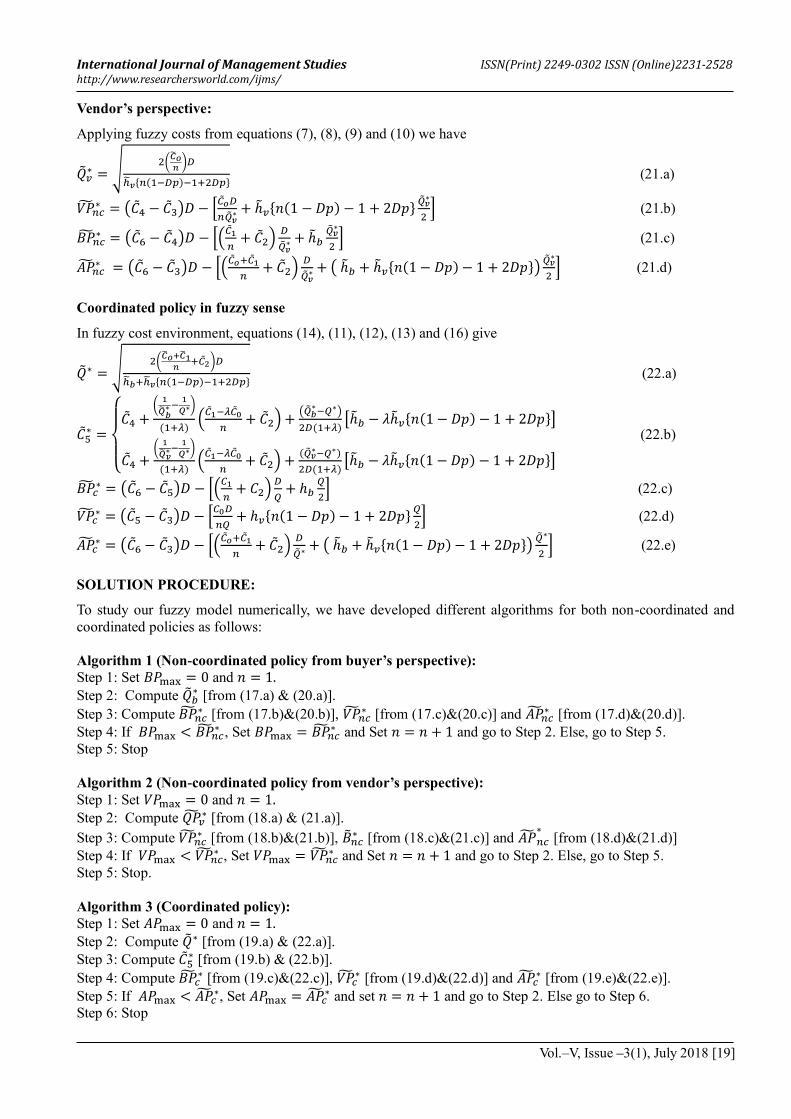
Vendor’s perspective:
Applying fuzzy costs from equations (7), (8), (9) and (10) we have
��𝑣∗ = √
2(��𝑜𝑛)𝐷
ℎ𝑣*𝑛(1;𝐷𝑝);1:2𝐷𝑝+ (21.a)
𝑉��𝑛𝑐∗ = (��4 − ��3)𝐷 − 0
��𝑜𝐷
𝑛��𝑣∗ + ℎ𝑣*𝑛(1 − 𝐷𝑝) − 1 + 2𝐷𝑝+
��𝑣∗
21 (21.b)
𝐵��𝑛𝑐∗ = (��6 − ��4)𝐷 − 0.
��1
𝑛+ ��2/
𝐷
��𝑣∗ + ℎ𝑏
��𝑣∗
21 (21.c)
𝐴��𝑛𝑐∗ = (��6 − ��3)𝐷 − 0.
��𝑜:��1
𝑛+ ��2/
𝐷
��𝑣∗ + ( ℎ𝑏 + ℎ𝑣*𝑛(1 − 𝐷𝑝) − 1 + 2𝐷𝑝+)
��𝑣∗
21 (21.d)
Coordinated policy in fuzzy sense
In fuzzy cost environment, equations (14), (11), (12), (13) and (16) give
��∗ = √2(
��𝑜+��1𝑛
:��2)𝐷
ℎ𝑏:ℎ𝑣*𝑛(1;𝐷𝑝);1:2𝐷𝑝+ (22.a)
��5∗ =
{
��4 +
(1
��𝑏∗;
1
𝑄∗)
(1:𝜆).��1;𝜆��0
𝑛+ ��2/ +
(��𝑏∗;𝑄∗)
2𝐷(1:𝜆)[ℎ𝑏 − 𝜆ℎ𝑣*𝑛(1 − 𝐷𝑝) − 1 + 2𝐷𝑝+]
��4 +(1
��𝑣∗;
1
𝑄∗)
(1:𝜆).��1;𝜆��0
𝑛+ ��2/ +
(��𝑣∗;𝑄∗)
2𝐷(1:𝜆)[ℎ𝑏 − 𝜆ℎ𝑣*𝑛(1 − 𝐷𝑝) − 1 + 2𝐷𝑝+]
(22.b)
𝐵��𝑐∗ = (��6 − ��5)𝐷 − 0.
𝐶1
𝑛+ 𝐶2/
𝐷
𝑄+ ℎ𝑏
𝑄
21 (22.c)
𝑉��𝑐∗ = (��5 − ��3)𝐷 − 0
𝐶0𝐷
𝑛𝑄+ ℎ𝑣*𝑛(1 − 𝐷𝑝) − 1 + 2𝐷𝑝+
𝑄
21 (22.d)
𝐴��𝑐∗ = (��6 − ��3)𝐷 − 0.
��𝑜:��1
𝑛+ ��2/
𝐷
��∗+ ( ℎ𝑏 + ℎ𝑣*𝑛(1 − 𝐷𝑝) − 1 + 2𝐷𝑝+)
��∗
21 (22.e)
SOLUTION PROCEDURE:
To study our fuzzy model numerically, we have developed different algorithms for both non-coordinated and
coordinated policies as follows:
Algorithm 1 (Non-coordinated policy from buyer’s perspective):
Step 1: Set 𝐵𝑃max = 0 and 𝑛 = 1. Step 2: Compute ��𝑏
∗ [from (17.a) & (20.a)].
Step 3: Compute 𝐵��𝑛𝑐∗ [from (17.b)&(20.b)], 𝑉��𝑛𝑐
∗ [from (17.c)&(20.c)] and 𝐴��𝑛𝑐∗ [from (17.d)&(20.d)].
Step 4: If 𝐵𝑃max < 𝐵��𝑛𝑐∗ , Set 𝐵𝑃max = 𝐵��𝑛𝑐
∗ and Set 𝑛 = 𝑛 + 1 and go to Step 2. Else, go to Step 5.
Step 5: Stop
Algorithm 2 (Non-coordinated policy from vendor’s perspective):
Step 1: Set 𝑉𝑃max = 0 and 𝑛 = 1. Step 2: Compute 𝑄��𝑣
∗ [from (18.a) & (21.a)].
Step 3: Compute 𝑉��𝑛𝑐∗ [from (18.b)&(21.b)], ��𝑛𝑐
∗ [from (18.c)&(21.c)] and 𝐴��𝑛𝑐∗
[from (18.d)&(21.d)]
Step 4: If 𝑉𝑃max < 𝑉��𝑛𝑐∗ , Set 𝑉𝑃max = 𝑉��𝑛𝑐
∗ and Set 𝑛 = 𝑛 + 1 and go to Step 2. Else, go to Step 5.
Step 5: Stop.
Algorithm 3 (Coordinated policy):
Step 1: Set 𝐴𝑃max = 0 and 𝑛 = 1. Step 2: Compute ��∗ [from (19.a) & (22.a)].
Step 3: Compute ��5∗ [from (19.b) & (22.b)].
Step 4: Compute 𝐵��𝑐∗ [from (19.c)&(22.c)], 𝑉��𝑐
∗ [from (19.d)&(22.d)] and 𝐴��𝑐∗ [from (19.e)&(22.e)].
Step 5: If 𝐴𝑃max < 𝐴��𝑐∗, Set 𝐴𝑃max = 𝐴��𝑐
∗ and set 𝑛 = 𝑛 + 1 and go to Step 2. Else go to Step 6.
Step 6: Stop
International Journal of Management Studies ISSN(Print) 2249-0302 ISSN (Online)2231-2528 http://www.researchersworld.com/ijms/
Vol.–V, Issue –3(1), July 2018 [20]
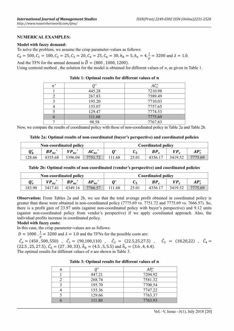
NUMERICAL EXAMPLES:
Model with fuzzy demand:
To solve the problem, we assume the crisp parameter-values as follows:
𝐶0 = 500, 𝐶1 = 100, 𝐶2 = 25, 𝐶3 = 20, 𝐶4 = 25, 𝐶6 = 30, ℎ𝑏 = 5, ℎ𝑣 = 4,1
𝑝= 3200 and 𝜆 = 1.0.
And the TFN for the annual demand is �� = (800 , 1000, 1200). Using centroid method , the solution for the model is obtained for different values of n, as given in Table 1.
Table 1: Optimal results for different values of 𝒏
𝑛∗ 𝑄∗ 𝐴𝐶𝑐∗
1 445.28 7210.98
2 267.83 7589.49
3 195.20 7710.03
4 155.07 7757.65
5 129.47 7774.53
6 111.68 7775.69
7 98.58 7767.83
Now, we compare the results of coordinated policy with those of non-coordinated policy in Table 2a and Table 2b.
Table 2a: Optimal results of non-coordinated (buyer’s perspective) and coordinated policies
Non-coordinated policy Coordinated policy
𝑸𝒃∗ 𝑩𝑷𝒏𝒄
∗ 𝑽𝑷𝒏𝒄
∗ 𝑨𝑪𝒏𝒄
∗ 𝑸∗ 𝑪𝟓 𝑩𝑷𝒄 𝑽𝑷𝒄 𝑨𝑷𝒄
∗
128.66 4355.68 3396.04 7751.72 111.68 25.01 4356.17 3419.52 7775.69
Table 2b: Optimal results of non-coordinated (vendor’s perspective) and coordinated policies
Non-coordinated policy Coordinated policy
𝑸𝒗∗ 𝑽𝑷𝒏𝒄
∗ 𝑩𝑷𝒏𝒄
∗ 𝑨𝑷𝒏𝒄
∗ 𝑸∗ 𝑪𝟓 𝑩𝑷𝒄 𝑽𝑷𝒄 𝑨𝑷𝒄
∗
183.90 3417.41 4349.16 7766.57 111.68 25.01 4356.17 3419.52 7775.69
Observation: From Tables 2a and 2b, we see that the total average profit obtained in coordinated policy is
greater than those were obtained in non-coordinated policy (7775.69 vs. 7751.72 and 7775.69 vs. 7666.57). So,
there is a profit gain of 23.97 units (against non-coordinated policy with buyer’s perspective) and 9.12 units
(against non-coordinated policy from vendor’s perspective) if we apply coordinated approach. Also, the
individual profits increase in coordinated policy.
Model with fuzzy costs: In this case, the crisp parameter-values are as follows:
𝐷 = 1000 , 1
𝑝= 3200 and 𝜆 = 1.0 and the TFNs for the possible costs are:
��𝑜 = (450 , 500, 550) , ��1 = (90,100,110) , ��2 = (22.5,25,27.5) , ��3 = (18,20,22) , ��4 =(22.5 , 25, 27.5), ��6 = (27 , 30, 33), ℎ𝑏 = (4.5 , 5, 5.5) and ℎ𝑣 = (3.6 , 4, 4.4). The optimal results for different values of n are shown in Table 3.
Table 3: Optimal results for different values of 𝒏
𝑛 𝑄∗ 𝐴𝑃𝑐∗
1 447.21 7204.92
2 268.74 7581.32
3 195.70 7700.54
4 155.36 7747.22
5 129.66 7763.37
6 111.80 7763.93
International Journal of Management Studies ISSN(Print) 2249-0302 ISSN (Online)2231-2528 http://www.researchersworld.com/ijms/
Vol.–V, Issue –3(1), July 2018 [21]
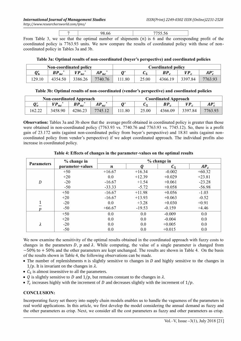
7 98.66 7755.56
From Table 3, we see that the optimal number of shipments (𝑛) is 6 and the corresponding profit of the
coordinated policy is 7763.93 units. We now compare the results of coordinated policy with those of non-
coordinated policy in Tables 3a and 3b.
Table 3a: Optimal results of non-coordinated (buyer’s perspective) and coordinated policies
Non-coordinated policy Coordinated policy
𝑸𝒃∗ 𝑩𝑷𝒏𝒄
∗ 𝑽𝑷𝒏𝒄
∗ 𝑨𝑷𝒏𝒄
∗ 𝑸∗ 𝑪𝟓 𝑩𝑷𝒄 𝑽𝑷𝒄 𝑨𝑷𝒄
∗
129.10 4354.50 3386.26 7740.76 111.80 25.00 4366.19 3397.84 7763.93
Table 3b: Optimal results of non-coordinated (vendor’s perspective) and coordinated policies
Non-coordinated Approach Coordinated Approach
𝑸𝒗∗ 𝑽𝑷𝒏𝒄
∗ 𝑩𝑷𝒏𝒄
∗ 𝑨𝑷𝒏𝒄
∗ 𝑸∗ 𝑪𝟓 𝑩𝑷𝒄 𝑽𝑷𝒄 𝑨𝑷𝒄
∗
162.22 3458.90 4286.23 7745.12 111.80 25.00 4366.09 3397.84 7763.93
Observation: Tables 3a and 3b show that the average profit obtained in coordinated policy is greater than those
were obtained in non-coordinated policy (7763.93 vs. 7740.76 and 7763.93 vs. 7745.12). So, there is a profit
gain of 23.172 units (against non-coordinated policy from buyer’s perspective) and 18.81 units (against non-
coordinated policy from vendor’s perspective) if we adopt coordinated approach. The individual profits also
increase in coordinated policy.
Table 4: Effects of changes in the parameter-values on the optimal results
Parameters % change in
parameter-values
% change in
𝒏 𝑸 𝑪𝟓 𝑨𝑷𝒄
𝐷
+50 +16.67 +16.34 -0.002 +60.32
+20 0.0 +12.39 +0.029 +23.81
-20 -16.67 +1.54 +0.061 -23.28
-50 -33.33 -5.72 +0.058 -56.98
1
𝑝
+50 -16.67 +11.98 +0.056 -1.03
+20 -16.67 +13.93 +0.063 -0.52
-20 0.0 +3.28 +0.030 +0.91
-50 +66.67 -19.53 -0.159 +4.46
𝜆
+50 0.0 0.0 -0.009 0.0
+20 0.0 0.0 -0.004 0.0
-20 0.0 0.0 +0.005 0.0
-50 0.0 0.0 +0.015 0.0
We now examine the sensitivity of the optimal results obtained in the coordinated approach with fuzzy costs to
changes in the parameters 𝐷, 𝑝 and 𝜆. While computing, the value of a single parameter is changed from
−50% to + 50% and the other parameters are kept unchanged. The results are shown in Table 4. On the basis
of the results shown in Table 4, the following observations can be made.
The number of replenishments 𝑛 is slightly sensitive to changes in 𝐷 and highly sensitive to the changes in
1/𝑝. It is invariant on the changes in 𝜆.
𝐶5 is almost insensitive to all the parameters.
𝑄 is slightly sensitive to 𝐷 and 1/𝑝, but remains constant to the changes in 𝜆.
𝑐 increases highly with the increment of 𝐷 and decreases slightly with the increment of 1/𝑝.
CONCLUSION:
Incorporating fuzzy set theory into supply chain models enables us to handle the vagueness of the parameters in
real world applications. In this article, we first develop the model considering the annual demand as fuzzy and
the other parameters as crisp. Next, we consider all the cost parameters as fuzzy and other parameters as crisp.
International Journal of Management Studies ISSN(Print) 2249-0302 ISSN (Online)2231-2528 http://www.researchersworld.com/ijms/
Vol.–V, Issue –3(1), July 2018 [22]
Here, we have used symmetric TFNs to represent the imprecise annual demand, set up cost, ordering cost,
transportation cost, per unit production cost, un-discounted per unit sell price of the vendor, per unit sell price of
the buyer, holding cost per unit per unit time for the vendor, holding cost per unit per unit time for the buyer and
derived the average profit of the system in fuzzy sense. We then applied centroid method for defuzzification of
the fuzzy profit. It is observed from the numerical study that the joint profit for the coordinated policy is higher
than those are obtained in the non-coordinated policy. This emphasizes that coordination between vendor and
buyer is very much essential to obtain better optimal results. The model may be extended by considering the
other parameters as fuzzy and different defuzzification methods may also be used to obtain the average profit in
crisp. Another extension of this work may be possible by allowing shortages in buyer’s inventory or considering
the production system imperfect.
REFERENCES:
Goyal, S.K. (1976). An integrated inventory model for a single-supplier single-customer problem. International Journal of Production Research, 15, 459-463.
Banerjee, A. (1988). A joint economic lot size model for purchaser and vendor. Decision Sciences, 17, 292-311.
Goyal, S.K. (1988). A joint economic lot size model for purchaser and vendor: a comment. Decision Sciences,19, 236-241.
Lu, L. (1995). A one-vendor multi-buyer integrated inventory model. European Journal of Operational Research, 81, 312-323.
Goyal, S.K. (1995). A one-vendor multi-buyer integrated inventory model: a comment. European Journal of
Operational Research, 81, 312-323. Hill, R.M.(1999). The optimal production and shipment policy for the single-vendor single-buyer integrated
production-inventory model. International Journal of Production Research, 37, 2463-2475.
Hogue, M.A. & Goyal, S.K. (2000). An optimal policy for a single vendor single buyer integrated production-inventory problem with capacity constraint of the transport equipment. International Journal of Production Economics, 65, 305-315.
Ben-Daya, M. & Hariga, M. (2004). Integrated single vendor single buyer model with stochastic demand and variable lead time. International Journal of Production Economics, 92, 75-80.
Li, J. & Liu, J. (2006). Supply chain coordination with quantity discount policy. International Journal of Production Economics, 101, 89-98.
Qin, Y., Tang, H. & Guo, C. (2007). Channel coordination and volume discounts with price sensitive demand .
International Journal of Production Research, 105, 43-53. Sajadieh, M.S., Akbari Jokar, M.R & Modarres, M. (2009). Developing a coordinated vendor-buyer model in two
stage supply chains with stochastic lead time. Computers and Operations Research, 36, 2484-2489.
Yang, M.F. (2010). Supply chain integrated inventory model with present value and dependent crashing cost is polynomial. Mathematical and Computer Modelling, 51, 802-809.
Masihabadi, S. & Eshghi, K. (2011). Coordinating a seller-buyer supply chain with a proper allocation of chain’s surplus profit using a general side payment contract. Journal of Industrial and System Engineering, 5, 63-79.
Shahrjerdi, R., Anuar, M.K., Mustapha, F., Ismail, N. & Esmaeili, M. (2011). An integrated inventory model under
cooperative and non-cooperative seller-buyer and vendor supply chain. African Journal of Business Management, 5, 8361-8367.
Saha, S., Das, S. & Basu, M.(2012). Supply chain coordination under stock and price-dependent selling rates under
declining market. Hindawi Publishing Corporation:Advances in Operations Research, doi-10.1155/2012/375128.
Moharana, H.S., Murty, J.S., Senapati, S.K. & Khuntia, K. (2012). Coordination, collaboration and integration for supply chain management. International Journal of Interscience Management Review, 2(2), 2012.
Shah, N.H., Patel, D.G. & Shah, D.B. (2013). Optimal pricing, shipments and ordering policies for single-supplier
single-buyer inventory system with price sensitive stock-dependent demand and order-linked trade credit. Global Journal of Researches in Engineering, 13(1), 2013.
Dey, O., Giri, B. C. (2014). Optimal vendor investment for reducing defect rate in a vendor buyer integrated system
with imperfect production process. International Journal of Production Economics, 155(1), 222–228. Zhang, Q., Luo, J., & Duan, Y. (2016). Buyer-vendor coordination for fixed lifetime product with quantity discount
under finite production rate. International Journal of Systems Science, 47(4), 821–834.
Li, J., Su, Q., & Ma, L. (2017). Production and transportation outsourcing decisions in the supply chain under single and multiple carbon policies. Journal of Cleaner Production, 141, 1109–1122.
Zadeh, L. (1965). Fuzzy sets. Information and Control, 8,338-353. Yao, J.S. & Lee, H.M. (1996). Fuzzy inventory with backorder for fuzzy order quantity. Information Science, 93,
International Journal of Management Studies ISSN(Print) 2249-0302 ISSN (Online)2231-2528 http://www.researchersworld.com/ijms/
Vol.–V, Issue –3(1), July 2018 [23]
283-319.
Yao, J.S. & Chiang, J. (2003). Inventory without backorder with fuzzy total cost and fuzzy storing cost defuzzified by centroid and signed distance. European Journal of Operational Research, 148(2), 401-409.
Chiang, J., Yao, J.S. & Lee, H.M. (2005). Fuzzy inventory with backorder defuzzification by signed distance method.
Journal of Information Science and engineering, 21,673-694. Tutunchu, G.Y., Akoz, O., Apaydin, A. & Petrovic, D. (2008). Continuous review inventory control in the presence of
fuzzy costs. International Journal of Production Economics, 113(2), 775-784.
Lin, Y.J. (2008). A periodic review inventory model involving fuzzy expected demand short and fuzzy backorder rate. Computers and Industrial Engineering, 54(3), 666-676.
Sadi-Nezhad, S., Nahavandi, S.M. & Nazeni, J. (2011). Periodic and continuous inventory models in the presence of
fuzzy costs. International Journal of Industrial Engineering Computations, 2, 167-178. Lee, H.M. & Lin, L. (2011). Applying signed distance method for fuzzy inventory without backorder. International
Journal of Innovative Computing, Information and Control, 7(6), 3523-3531. Sarkar, S. & Chakrabarti, T. (2012). An EPQ model with two-component demand under fuzzy environment and
Weibull distribution deterioration with shortages. Hindawi Publishing Corporation, Mathematical Problems
in Engineering, doi:10.1155/2012/264182. Mahapatra, N.K., Bera, U.K. & Maiti, M. (2012). A production inventory model with shortages, fuzzy preparation
time and variable production and demand. American Journal of Operational Research, 2, 183-192.
Mahata, G., Goswami, A. & Gupta, D. (2005). A joint economic-lot-size model for purchaser and vendor in fuzzy sense. Computers and Mathematics with Applications, (10-12):1767-1790.
Corbett, C. & Groote, X. (2000). A supplier’s optimal quantity discount policy under asymmetric information. Management Science, 46,444-450.
Petrovic, D., Roy, R. & Petrovic, R. (1999). Supply chain modelling using fuzzy sets. International Journal of
Production Economics, 59(1-3), 443-453. Gunasekaran, N., Rathesh, S., Arunachalam, S. & Koh, S.C.L. (2006). Optimizing supply chain management using
fuzzy approach. Journal of Manufacturing Technology Management, 17(6), 737-749.
Sucky, E. (2006). A bargaining model with asymmetric information for a single supplier-single buyer problem. European Journal of Operational Research, 171(2), 516-535.
Ganga, G.M.D. & Carpinetti, L.C.R. (2011). A fuzzy logic approach to supply chain performance management.
International Journal of Production Economics, 134, 177-187. Costantino, N., Dotoli, M., Falagario, M., Fanti, M.P. & Mangini, A.M. (2012). A model for supply management of
agile manufacturing supply chains. International Journal of Production Economics, 135, 451-457. Sinha, S. & Sarmah, S.P. (2008). An application of fuzzy set theory for supply chain coordination. International
Journal of Management Science and Engineering Management, 3(1), 19-32.
Taleizadeh, A. A., Niaki, S. T. A., & Wee, H. M. (2013). Joint single vendor-single buyer supply chain problem with stochastic demand and fuzzy lead-time. Knowledge-Based Systems, 48, 1–9.
Mahata, G. C. (2015). An integrated production-inventory model with backorder and lot for lot policy in fuzzy sense.
International Journal of Mathematics in Operational Research, 7, 69–102. Priyan, S., & Uthayakumar, R. (2016). Economic design of multi-echelon inventory system with variable lead time
and service level constraint in a fuzzy cost environment. Fuzzy Information and Engineering, 8, 465–511. Jauhari, W. A. & Saga, R. S. (2017) A stochastic periodic review inventory model for vendor–buyer system with
setup cost reduction and service–level constraint. Production & Manufacturing Research, 5:1, 371-389.
----