A spatial analysis of international stock market linkages

Hossein Asgharian, Wolfgang Hess and Lu Liu*

Department of Economics, Lund University

Box 7082, S-22007 Lund, Sweden.

 

Work in progress

Abstract

The severe global impacts of the recent financial crises have intensified the need to understand how country specific shocks are transmitted to other countries. Using spatial econometrics techniques, we analyze to what extent various linkages between countries affect the interdependence of their stock markets. We analyze a number of different linkages: geographical neighborhood, similarity in industrial structure, economic integration (measured by the degree of countries’ bilateral trade and bilateral foreign direct investment) and monetary integration (measured by the closeness of countries’ inflation rates and the stability of their bilateral exchange rate). We analyze both return and return volatility of country indexes for a large sample of 41 countries over a period of 16 years. Our empirical results indicate that economic factors affect the dependencies among financial markets to a greater extent than geographical neighborhood or monetary integration. In particular, we find that a country’s market return and volatility depend to a large degree on market returns and volatilities in countries that are similar in industrial structure and those that are important trading partners. By identifying several linkages through which stock markets are connected with each other and assessing the relative importance of these linkages, we provide new insights which can be used by financial investors for risk hedging through global diversification.

 

                                                            * Tel.: +46 46 222 8667; fax: +46 46 222 4118. E-mail address: Hossein.Asgharian@nek.lu.se; Wolfgang.Hess@nek.lu.se; Lu.Liu@nek.lu.se We are very grateful to Jan Wallanders och Tom Hedelius stiftelse and Bankforskningsinstitut for funding this research.

1. Introduction

The severe global economic impacts of the recent financial crises have intensified the

needs for modeling linkages between different financial markets. It is important for

financial investors to understand how country (market) specific shocks are transmitted to

other countries (markets), because it affects their ability of risk hedging through global

diversification.

Interactions among international stock markets have been studied by a number of earlier

studies. Some studies, e.g. Erb et al. (1994), Longin and Solnik (1995), and Karolyi and

Stulz (1996), have focused on correlations between stock market returns, while others,

e.g. Bekaert and Harvey (1995, 1997), Bekaert et al. (2005), Asgharian and Bengtsson

(2006) and Asgharian and Nossman (2011), have addressed the issue of risk spillover

across markets. The majority of previous studies have solely focused on assessing the

degree of dependence among markets, whereas the channels through which stock markets

are related to each other have usually been ignored.

Exploring the underlying economic structures which affect the co-movements of financial

markets helps us to properly assess the sensitivity of the markets to exogenous shocks.

The recent developments in spatial econometrics provide appropriate tools for analyzing

this subject. Applying spatial econometrics makes it possible to incorporate factors

related to location and distance in the analysis. Using this approach, the structure of the

relationship between observations at different locations will be connected to the relative

position of the observations in a hypothetical space, for example the geographical

location of a country. We employ these tools to investigate which attributes affect the

transmission of shocks among different markets. Our aim is to identify to what extent

different linkages between markets affect the degree of market co-movements.

We use different attributes to map the spatial location (distance/closeness) of financial

markets and analyze the degree of spatial dependence among them. The existence of

spatial dependence can be motivated by two different concepts, one that relies on omitted

explanatory variables and a second that is based on spatial spillovers stemming from

contagion effects (see e.g. LeSage and Pace (2009)). Our study focuses on the latter

concept.

We analyze a number of different linkages: geographical neighborhood, similarity in

industrial structure, economic integration (measured by the degree of countries’ bilateral

trade and bilateral foreign direct investment) and monetary integration (measured by the

closeness of countries’ inflation rates and the stability of their bilateral exchange rate).

We analyze both return and return volatility of country indexes for a large sample of 41

countries over a period of 16 years.

Our empirical results indicate that economic factors affect the dependencies among

financial markets to a greater extent than geographical neighborhood or monetary

integration. In particular, we find that a country’s market return and volatility depend to a

large degree on market returns and volatilities in countries that are similar in industrial

structure and those that are important trading partners.

To our knowledge this is the first in-depth analysis of the underlying economic structure

of global stock market interactions. By identifying several linkages through which stock

markets are connected with each other and assessing the relative importance of these

linkages, we provide new insights which can be used by financial investors for risk

hedging through global diversification. A critical issue in risk management is to obtain a

precise estimate of the future correlation between markets. The estimate is sensitive to the

choice of methods and the length of the estimation sample. Our results can be used as

additional information to improve correlation prediction when making investment

decisions.

The remainder of the paper is organized as follows. Section 2 presents the spatial

econometrics methods used in this paper. Section 3 describes the data sources and the

model specifications used the empirical analysis. Section 4 contains the empirical results,

and Section 5 concludes the paper.

2. Econometric Modeling

The concept of spatial dependence in regression models reflects a situation where values

of the dependent variable at one location depend on the values of neighboring

observations at nearby locations. Such dependencies can originate from e.g. spatial

spillovers stemming from contagion effects or from unobserved heterogeneity caused by

omitted explanatory variables. Depending on the source of the spatial correlation, a

variety of alternative spatial regression structures can arise. The two most commonly

applied spatial regression models are the spatial autoregressive (SAR) model and the

spatial error model. The latter models spatial dependence in the disturbances and the

former tackles the problem of spatial correlation by including linear combinations of the

dependent variable (so-called spatial lags) as additional regressors. One fundamental

limitation of spatial error models is that these models rule out spillover effects by

construction (see e.g. LeSage and Pace, 2009). Since risk spillovers have an important

effect on the dependencies among financial markets, our empirical analysis relies solely

on the SAR model.1

Formally, we consider the following SAR specification with two spatial lags:

⊗ ⊗ , (1)

where and are spatial autoregressive parameters, and and are (possibly

time-varying) spatial weights matrices describing the spatial arrangement of the cross

section units. The dimension of and is N×N, where N is the number of cross-

sectional observations in the sample. The model specification above is expressed in

stacked matrix form. The vector contains NT observations of the dependent variable

(monthly volatility or monthly return), where T is the time-series dimension. Similarly,

is a NT×k-matrix containing the stacked observations on k explanatory variables

(including individual-specific intercepts) and is the corresponding k×1-vector of

parameters. Finally, is an NT×1-vector of idiosyncratic error terms, is an identity

matrix of dimension T, and ⊗ denotes the Kronecker product.

The distinctive feature of the SAR model is that it contains linear combinations of the

dependent variable as additional explanatory variables. This induces an endogeneity

problem which renders conventional OLS estimates of the model parameters inconsistent.

Maximum likelihood estimation can be used as an alternative to OLS that yields

                                                            1 Anselin (1988) also provides a persuasive argument that the focus of spatial econometrics should be on modeling the effects of spillovers.  

consistent parameter estimates. The log-likelihood function that is to be maximized is

given by

ln L ∑ ln | | ln 2 ′ (2)

Where

⊗ ⊗

and is the error variance that is to be estimated along with the structural model

parameters (see e.g. Anselin, 2006). Maximizing the likelihood function above is not

equivalent to minimizing the sum of squares as in the conventional linear regression

model. The crucial difference is the presence of the log-Jacobian terms

ln | |.

This illustrates why OLS does not yield consistent estimates of the SAR model

parameters. The log-Jacobian terms also impose constraints on the parameter space for

and , which must be such that

| | 0.

Since this study focuses on the identification of linkages through which shocks are

transmitted across markets, the specification of and is of crucial importance. In

our empirical analysis we have defined these matrices in a way that allows for

asymmetric dependencies between any pair of markets. In specifying and we

start out with constructing a Boolean contiguity matrix that indicates for any pair of

markets in the sample whether market is a neighbor to market according to various

definitions of neighborhood.2 The element in the th row and the th column of takes on

the value one if market is contiguous to market , and zero otherwise. For each market ,

the 50% of remaining markets that are closest according to the respective definition of

neighborhood are considered to be neighbors. Similarly, we construct a Boolean matrix

with individual elements equal to one if market is not a neighbor to market . Formally,

this matrix is computed as

,

where is an N×N-matrix of ones and is an identity matrix of dimension N. The spatial

weights matrices and are then obtained by row-standardization of and ,

respectively.

Using an SAR(2) model with spatial weights matrices as defined above has two

noteworthy implications. First, this model specification allows us to directly compare the

spatial dependencies existing among neighbors with those existing among non-neighbors.

Second, our specification of and allows for asymmetric dependencies between

any pair of markets. For example, when defining neighborhood based on the amount of

bilateral trade, the U.S. are contiguous to the Philippines, since the volume of trade

between the Philippines and the U.S. is above the median volume of trade between the

Philippines and all other countries. The Philippines, however, are not a first-order

neighbor to the U.S., since their bilateral trade is below the median volume of trade

between the U.S. and all other countries.

Although the focus of this study is on spatial dependencies among markets, we also

account for spatial heterogeneity among markets by including a number of fundamental

                                                            2 The various definitions of neighborhood are explained in detail in Section 3. 

explanatory variables, which may affect market returns and volatilities, in the model. A

number of researchers have noted that SAR models require special interpretation of the

-parameters associated with these explanatory variables (see e.g. Anselin and LeGallo,

2006, or Kelejian et al., 2006). In essence, is no longer equivalent to the marginal

effects of changes in the fundamentals. The reason for this is that a change in

fundamentals in one country, say country i, affects the volatility of that country, which in

turn affects the volatilities at nearby locations, which then feed back to the volatility of

country i. The values of should thus be interpreted as average immediate effects of

changes in the explanatory variables, which do not include such spill-over and feedback

effects.

3. Methodology and Data

This section describes the selected channels of spatial dependence, i.e. financial

integration, economic integration and geographical closeness. For each channel, we

define spatial distances among markets and hence the contiguity matrix. In addition, we

present the selected control variables included in the model. We also make prior

predictions on their signs of impact on market returns and volatility. The remained part of

this section describes data sources.  

3.1. Potential channels of spatial dependence

We use three types of bilateral factors capturing the relative distance/closeness of the

financial markets to one another, in order to investigate the determinants of the degree of

dependence among different markets. The first type defines financial integration, among

them: exchange rate volatility, absolute difference between inflations. The second type

captures economic linkages (e.g. bilateral trade, bilateral foreign direct investment and

similarity of industrial structure). The third type is distance between capital cities, which

describes geographical distance.

3.1.1 Financial factors

Exchange rate volatility

An environment with stable exchange rates should reduce cross-currency risk premiums

and imply more similar discount rates. This should give a more homogenous valuation of

equities and increase incentives to invest in foreign markets. Hence a less volatile

exchange rate is expected to increase the degree of dependence. (see for example Bekaert

and Harvey (1995) and Baele (2005)). We estimate exchange rate volatility as standard

deviation of daily bilateral exchange rates in each month.

Absolute difference between expected inflations

Absolute difference between expected inflation of two countries measures the degree of

monetary integration across the countries. Convergence of expected inflation should

imply an environment with stable exchange rates and increase incentives to invest in

foreign markets. Inflation is measured as CPI CPI /CPI for month t. Assuming

the series of inflation to be martingale, we estimate the expected inflation in month t as

the realized inflation in month t 1.

3.1.2 Economic factors

Bilateral trade

Large value of trade between two countries should imply higher dependence between the

countries and increase the degree of dependence. The variable of bilateral trade for

country with country in year is calculated as

,, ,

∑ , ∑ ,

where , is the value of export from country to country in year , and

, is the value of import to country from in year . In this way, , implies

the value of trade between country and country relative to the total value of trade

between country and all the countries except itself.

Bilateral foreign direct investment

Large value of bilateral FDI implies higher degree of exposures across the countries. The

variable of bilateral FDI is calculated in the same manner as the variable of bilateral

trade:

,, ,

∑ , ∑ ,

where , is the position of FDI outflow from country to country in year ,

and , is the position of FDI inflow to country from country in year .

Similarity in industrial structure

Countries with similar industrial structures are exposed to the same type of business risks.

To construct a proxy for this factor, we can for example use the countries' exposures to

the ten world industry indexes. Same as Asgharian and Bengtsson (2006), we use the

average absolute difference in exposures as a measure of the industry differences between

every pair of countries.

3.1.3 Geographic factor

Countries often have similar market structure and close economic relations with the

nearby countries. It is plausible that the market volatility of a country affects its nearby

countries to a larger extent. We use distances between capital cities to measure

geographical distances between countries.

3.2. Defining neighborhood

We use the medians of the bilateral variables (defined in section 3.1) of each market with

other markets as benchmarks to define the neighbors of that market. For exchange rate

volatility, absolute difference in expected inflation and similarity in industrial structure,

small values should imply closeness between markets. Therefore, if the value is smaller

than the median, these two countries are assumed to be neighbors. For bilateral trade,

bilateral FDI and geographical distance, values of variables larger than median imply

contiguity.

3.3. Selection of control variables

In addition to assessing the spatial dependence of different markets using the attributes

above, a number of explanatory macro variables are included in the model. These

variables are changes in exchange rate, unexpected inflation, sovereign default rate and

GDP growth. These variables are related to a country’s business cycle and can affect the

domestic equity market.

The change in exchange rate is calculated as the monthly difference of a country’s

exchange rate to USD. A positive change in exchange rate implies depreciation of this

country’s local currency, and is thus a proxy for economic distress. Therefore, we expect

the change in exchange rate to have a negative impact on market returns and a positive

impact on market volatility.

Unexpected inflation is computed as realized inflation minus expected inflation described

in Section 3.1. Positive unexpected inflation indicates economic boom, and can therefore

be expected to have a positive impact on market returns and a negative impact on

volatility.

Sovereign default rate is measured on an ordinal scale between 1(AAA) and 20(CC)

according to the Standard & Poor’s foreign currency rating. A rise in sovereign default

rate increases uncertainty and risk premium, so it should have a positive effect on market

volatility and returns.

3.4. Data Sources

We extract monthly and daily stock market indexes from MSCI from the end of 1994 to

October 29, 2010 and construct the monthly returns and daily returns by taking log

difference of the corresponding indexes. We construct the monthly returns by taking log

difference of the monthly indexes. The market volatility is estimated as standard

deviation of daily returns in each month.

We draw exchange rates from January 1995 to October 2010 from GTIS and

WM/Reuters. The data are extracted from Datastream. We extract monthly CPI3 from

Datastream over the period January 1995 to October 2010.

As for measure of industrial similarity, we collect the ten world industry indexes from

Datastream. We get the exposure of a market to the world industry by regressing the

returns of the market on the log-returns of each world industry index.

Data of bilateral trade is drawn from STAN Bilateral Trade Database (source: OECD).

The database presents the values of annual imports and exports of goods for all OECD

counties and seventeen non-OECD countries, broken down by partner countries, thus

providing data for all the countries in our study. The data covers the period 1995 to 2009.

The values are presented in US dollars at current prices. We assume that the observations

in 2010 the same with those in 2009.

Data of foreign direct investment positions is collected from International Direct

Investment Statistics (source: OECD). The Source provides annual bilateral FDI

positions in U.S. dollars over the period 1995 to 2009. It reports the positions of outward

FDI from OECD countries to OECD countries and non-OECD countries, as well as the

positions of outward FDI from non-OECD countries to OECD countries. However, some

observations are confidential. In addition, the observations on FDI from non-OECD

countries to non-OECD countries are missing. We treat the values of the non-available

observations as zeros.

                                                            3 CPI of Australia and New Zealand are not reported at monthly basis. We interpolate the reported quarterly CPI of Australia and New Zealand into the monthly series.    

We collect data of foreign direct investment positions from OECD International Direct

Investment Statistics. The Source provides annual bilateral FDI positions in U.S. dollars

over the period 1995 to 2008. We relate the It reports the positions of outward FDI from

OECD countries to OECD countries and non-OECD countries, as well as the positions of

outward FDI from non-OECD countries to OECD countries. The observations on FDI

from non-OECD countries to non-OECD countries are missing, however, the values of

these observations are minor so we treat them as zeros. The data for foreign currency

rating are collected from the Standard & Poor’s Sovereign Rating and the yearly gross

domestic product are from the World Bank.

4. Data Description

There are 41 equity markets in our spatial analysis. Table 1 presents the selected markets

and the descriptive statistics of their monthly returns over the period January 1995 to

October 2010. A first observation is that Turkey has the largest returns on average. The

maximum observation of Turkey is also the largest among all the markets. In comparison,

Ireland has the smallest returns on average. Judge from standard deviation and range,

Russian market has the highest level of risk, whereas the U.K. and the U.S. have

relatively small risk. In addition, levels of skewness show that Korea has the fewest

observations above its average while Belgium has the fewest observations below its

average. Belgium also has the highest probability of extreme values. Japan is almost

mesokurtotic.

[Insert Table 1]

In order to obtain some prior knowledge of relationships among the selected markets, we

present a world map depicting the monthly return correlations of the selected equity

markets with the U.S market (see Figure 1).

[Insert Figure 1]

To give a simple illustration of our neighborhood matrices, we in Table 2 present the

neighborhood of different markets with the US market according to the different factors.

In this table the entire sample is divided in two sub-periods, from 1995 to 2002 and from

2003 to 2010, respectively. We use the average value of the variables over each sub-

period to define the neighborhood. We use the medians of the bilateral variables of each

market with the US as benchmarks, thereby 50% of the countries are assumed to be

neighbor with the US.

Canada, Hong Kong, Singapore and the UK, are related to the US based on most of the

variables. On the other hand, some countries, such as Turkey, Russia and Czech republic,

are quite weekly related to the US. According to the several variables, India has become

closer to the US in the second period.

Table 3 reports the proportion of overlapping ones between each pair of neighborhood

matrices. Under the null-hypothesis that two different concepts of neighborhood are

independent, the expected proportion is 0.5. A value of zero indicates that the respective

definitions of neighborhood exhibit a perfectly negative correlation (neighborhood

according to one definition implies non-neighborhood according to the other one). A

value equal to one, on the other hand, indicates that the respective neighborhood

definitions have a perfectly positive correlation (neighborhood according to one

definition implies neighborhood according to the other one).

The table shows that almost all proportions are significantly different from 0.5, which

indicates that there are systematic relationships between the various neighborhood

definitions. However, the fractions are not particularly large, which shows that there are

noticeable differences among the various neighborhood matrices. It is therefore

worthwhile to separately analyze the dependencies among stock markets at proximate

locations for each specific concept of neighborhood.

5. Empirical Analysis

We analyze the spatial dependence among our selected markets over the entire sample

period of January 1995 to October 2010. In order to rank the factors by their effects on

spatial dependence, we not only investigate value and statistical significance of spatial

autocorrelation coefficients, but also examine whether the spatial relationships defined by

the selected factors outperform most of the possible spatial relationships. Furthermore,

we compare the selected factors pair-wise by incorporating two factors simultaneously

into the econometric model. In addition, in order to examine the changes in the spatial

dependence over time, we divide the sample into two sub-samples, where the first sub-

period is from January 1995 to November 2002 and the second sub-period is from

December 2002 to October 2010. In addition, to investigate if the relationship among

markets differs during a global distress periods comparing to the normal periods, we

divide the sample based on the level of the monthly world volatility, using the volatility

of the U.S. market as a proxy for the world-wide volatility. The high volatility period

includes months when the volatility is higher than the median; whereas the low volatility

period includes the remainder.

5.1. Estimated results over the entire sample period

We present the empirical results for returns and volatility over the entire sample period in

Table 4. The estimated :s of all the factors are highly significant and positive, implying

positive spatial dependence among markets within the defined neighborhoods. Judging

from the values of :s, we find that the ranking of factors for dependence among market

returns is similar to the ranking for volatility. For example, markets that are close in

terms of economic integration (except bilateral direct foreign investment) have larger

dependence with one another in both returns and volatility than markets that are

financially integrated or geographically close. Among all, the value of :s for industrial

structure are the highest (0.92 for returns, and 1.10 for volatility), implying that markets

similar in industrial structure tend to have the highest degree of spatial dependence. The

second important factor is bilateral trade. As for the financial factors, exchange rate

volatility plays a more important role in market dependence than expected inflation for

both returns and volatility. The result is however mixed for geographical distance. It has a

stronger effect than financial factors on volatility dependence, whereas it is worse than

exchange rate volatility in explaining return dependence. We find bilateral foreign direct

investment to be the worst factor in capturing spatial autocorrelation. This mainly results

from the low quality of the data for foreign direct investment, which makes the contiguity

matrix a bad measure of market relationships. In addition, because observations between

several markets and many of their partner countries are missing, these markets have

fewer than 20 neighbors, thus resulting in a smaller number of ones in the contiguity

matrix compared with other factors. Therefore, the estimated tends to be smaller.

[Insert Table 4]

In addition to :s, we also present the estimated :s that imply the degrees of spatial

dependence among non-neighboring markets. For all the factors except foreign direct

investment, the values of :s are much smaller than their corresponding :s. This is

consistent with our expectation that neighboring markets have higher degree of

dependence with one another than non-neighboring markets. However, we still find

positive spatial dependence within most of the defined neighborhoods, as the values of

:s are mostly positive. Only for industrial structure, is negative, implying negative

spatial autocorrelation among markets with different industrial structures. The value

for foreign direct investment is relatively large compared with the corresponding of .

This may result from the low quality of the data for foreign direct investment, which

makes the contiguity matrix a bad definition of relationships among markets and also

leads to larger number of ones in ̅ than in .

Furthermore, we find that the coefficients of most control variables are highly significant

for both returns and volatility, except the coefficient of GDP growth for returns. This

indicates that, in addition to spatial dependence, there is also significant spatial

heterogeneity in returns and volatility among the selected markets. The signs of the

coefficients are mostly consistent with the expectations discussed in section 3.3. For

instance, a positive change of exchange rate has immediate positive impact on the market

returns and negative impact on volatility.

In addition, estimated is also presented. is the conditional mean of the U.S return or

volatility, due to the inclusion of dummy variables for all the other markets. The

estimated of returns is negative and insignificant for most of the factors, implying that

the market returns can be mostly explained by spatial dependence and the control

variables. Only for industrial structure do we find to be statistically significant. As for

volatility, the estimated is also negative for all the factors, however, it’s statistically

significant for most of the factors except expected inflation and geographical distance.

5.2. Evaluating the defined neighborhood

As argued previously in this paper, the global trend international equity markets may

result in positive spatial dependence even among markets that are not neighbors to one

another. Therefore, in addition to examining the statistical significance of and , we

also evaluate whether the spatial neighborhoods defined by the selected factors

outperform other possible definitions of neighborhood. We randomly generate 200

contiguity matrices that have the same number of ‘ones’ as our selected contiguity matrix

and obtain 200 pairs of estimated and from the random matrices. Figures 2 and 3

depict the estimated values of :s and :s corresponding to our six selected

neighborhood factors for returns and volatility, respectively. They also show the lower

and upper 1%, 2.5% and 5% quantiles of the empirical distributions of and

obtained from 200 randomly generated W-matrices.

[Insert Figure 2 and Figure 3]

As for returns, :s lie above the upper 1% quantile of the empirical distribution for all

the factors except foreign direct investment. This suggests that these factors are better

than 99% possible measures of market relationships in capturing the spatial dependence

among our selected markets. In addition, the estimated :s are below the lower 1%

quantile of the empirical distribution for these factors, implying that the markets that are

non-neighboring according to the selected factors have small degrees of spatial

dependence compared with other possible definitions of neighborhood.

As for volatility, only for the economic factors (excluding foreign direct investment) are

economically significant above 1% upper quantile. The estimated for exchange rate

volatility and geographical factor are between 2.5% upper quantile and 5% upper

quantile. The estimated for expected inflation and foreign investment are not

economically significant.

5.3. Comparison among factors

In order to compare the bilateral factors explicitly with one another and rank them in

terms of their importance to spatial dependence, we modify the econometric modeling by

defining in a different way. We have the weighting matrix of one factor as and the

weighting matrix of another factor as . In this way, we are able to compare factors

pair-wise within the model. The factor with larger value of is better at explaining the

dependence among markets relative to the other factor.

We present the pair-wise comparison between factors by displaying the signs of

differences between and in Table 5. A positive sign shows that the factor in that

column has larger value of compared with the factor in the row. The comparison

between factors presented in Table 5 is consistent with the previous findings in Section

4.1 and 4.2. For example, we find that industrial structure is superior to all the other

factors in capturing dependence among both returns and volatility, as the difference

between its between those of all other factors are positive. Bilateral trade is the second

important factor, as it is inferior only to industrial structure. Geographical distance is

better than the financial factors and foreign direct investment in explaining volatility

dependence, whereas it is less important than exchange rate volatility for dependence

among market returns.

[Insert Table 5]

5.4. Sub-period analysis

In this section, we present the estimated :s for two sub-sample periods. As presented in

Table 6, we find that the spatial dependence in returns tend to be higher during the first

half of the sample period (until November 2002) than during the second half. With

respect to the spatial dependence in volatilities, the picture is not as clear: Our results

shown in Table 7 indicate that dependence in volatility among markets that are close in

terms of economic integration or geographical distance are larger during the second half

of the observation period, whereas dependence in volatility among markets that are close

in terms of financial integration are larger during the first half of the sample period.

Nevertheless, the ranking of the factors is still robust to the choice of sub-samples for

both returns and volatility.

[Insert Table 6 and Table 7]

6. Summary and Conclusions

In this study we have analyzed dependence among financial markets with respect to both

market returns and volatilities. We have applied spatial autoregressive models to

investigate the linkages through which markets are connected with each other.

Specifically, we have used monthly data on returns and volatilities for 41 markets

between January 1995 and October 2010 to assess six factors which potentially affect the

dependence among markets. Except geographical neighborhood, which is typically

assumed to affect spatial dependence, we have also considered three economic factors

(bilateral trade, bilateral FDI, and similarity in industrial structure) and two financial

factors (exchange rate volatility and differences in expected inflation) as potential sources

of spatial dependence.

Our main finding is that economic factors affect the dependence among financial markets

to a greater extent than geographical neighborhood or financial integration. In particular,

we find that a country’s market return and volatility depend to a large degree on market

returns and volatilities in countries that are similar in industrial structure and those that

are important trading partners.

We also find that, with respect to returns, the dependence among markets tend to be

higher during the first half of the sample period (until November 2002) than during the

second half. With respect to market volatilities, the picture is not as clear.

References

Anselin, L.,1988, Spatial Econometrics: Methods and Models, Dordrecht: Kluwer

Academic Publishers.

Anselin, L., 2006, Spatial econometrics, in: T.C. Mills and K. Patterson (Eds.), Palgrave

Handbook of Econometrics: Volume 1, Econometric Theory. Basingstoke, Palgrave

Macmillan, pp.901-969.

Anselin, L. and J. Le Gallo, 2006. Interpolation of air quality measures in hedonic house

price models: Spatial aspects, Spatial Economic Analysis 1, 31-52.

Asgharian, H., Bengtsson, C., 2006. Jump spillover in international equity markets,

Journal of Financial Econometrics 4, 167–203.

Asgharian, H., Nossman, M., 2011. Risk Contagion among international stock markets,

Journal of International Money and Finance 28, 22-38.

Baele, L., 2005. Volatility spillover effects in European equity markets, Journal of

Financial and Quantitative Analysis 40, 373–401.

Bekaert, G., Harvey, C.R., 1995. Time-varying world market integration. Journal of

Finance 50, 403–444.

Bekaert, G., Harvey, C.R., 1997. Emerging equity market volatility. Journal of Financial

Economics 43, 29–77.

Bekaert, G., Harvey, C. R., Ng, A., 2005. Market integration and contagion. Journal of

Business 78, 39–69.

Erb, C., Harvey, C.R., Viskanta, T., 1994. Forecasting international equity correlations.

Financial Analysts Journal 50, 32–45.

Karolyi, G.A., Stulz, R.M., 1996. Why do markets move together? An investigation of

U.S.–Japan stock return comovements. Journal of Finance 51, 951–986.

Kelejian, H.H., Tavlas, G.S., Hondronyiannis, G., 2006. A spatial modeling

approach to contagion among emerging economies. Open Economies

Review 17, 423-442.

LeSage, J., Pace, R.K., 2009, Introduction to Spatial Econometrics, Boca Raton:

Chapman & Hall/CRC.

Longin, F., Solnik, B., 1995. Is correlation in international equity returns constant: 1960–

1990. Journal of International Money and Finance 14, 3–26.

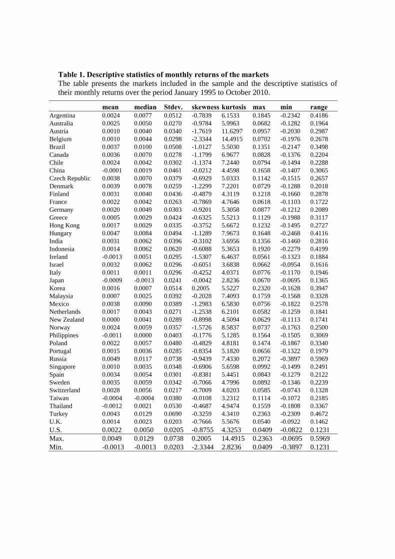
Table 1. Descriptive statistics of monthly returns of the markets The table presents the markets included in the sample and the descriptive statistics of their monthly returns over the period January 1995 to October 2010.

mean median Stdev. skewness kurtosis max min range Argentina 0.0024 0.0077 0.0512 -0.7839 6.1533 0.1845 -0.2342 0.4186 Australia 0.0025 0.0050 0.0270 -0.9784 5.9963 0.0682 -0.1282 0.1964 Austria 0.0010 0.0040 0.0340 -1.7619 11.6297 0.0957 -0.2030 0.2987 Belgium 0.0010 0.0044 0.0298 -2.3344 14.4915 0.0702 -0.1976 0.2678 Brazil 0.0037 0.0100 0.0508 -1.0127 5.5030 0.1351 -0.2147 0.3498 Canada 0.0036 0.0070 0.0278 -1.1799 6.9677 0.0828 -0.1376 0.2204 Chile 0.0024 0.0042 0.0302 -1.1374 7.2440 0.0794 -0.1494 0.2288 China -0.0001 0.0019 0.0461 -0.0212 4.4598 0.1658 -0.1407 0.3065 Czech Republic 0.0038 0.0070 0.0379 -0.6929 5.0333 0.1142 -0.1515 0.2657 Denmark 0.0039 0.0078 0.0259 -1.2299 7.2201 0.0729 -0.1288 0.2018 Finland 0.0031 0.0040 0.0436 -0.4879 4.3119 0.1218 -0.1660 0.2878 France 0.0022 0.0042 0.0263 -0.7869 4.7646 0.0618 -0.1103 0.1722 Germany 0.0020 0.0049 0.0303 -0.9201 5.3058 0.0877 -0.1212 0.2089 Greece 0.0005 0.0029 0.0424 -0.6325 5.5213 0.1129 -0.1988 0.3117 Hong Kong 0.0017 0.0029 0.0335 -0.3752 5.6672 0.1232 -0.1495 0.2727 Hungary 0.0047 0.0084 0.0494 -1.1289 7.9673 0.1648 -0.2468 0.4116 India 0.0031 0.0062 0.0396 -0.3102 3.6956 0.1356 -0.1460 0.2816 Indonesia 0.0014 0.0062 0.0620 -0.6088 5.3653 0.1920 -0.2279 0.4199 Ireland -0.0013 0.0051 0.0295 -1.5307 6.4637 0.0561 -0.1323 0.1884 Israel 0.0032 0.0062 0.0296 -0.6051 3.6838 0.0662 -0.0954 0.1616 Italy 0.0011 0.0011 0.0296 -0.4252 4.0371 0.0776 -0.1170 0.1946 Japan -0.0009 -0.0013 0.0241 -0.0042 2.8236 0.0670 -0.0695 0.1365 Korea 0.0016 0.0007 0.0514 0.2005 5.5227 0.2320 -0.1628 0.3947 Malaysia 0.0007 0.0025 0.0392 -0.2028 7.4093 0.1759 -0.1568 0.3328 Mexico 0.0038 0.0090 0.0389 -1.2983 6.5830 0.0756 -0.1822 0.2578Netherlands 0.0017 0.0043 0.0271 -1.2538 6.2101 0.0582 -0.1259 0.1841 New Zealand 0.0000 0.0041 0.0289 -0.8998 4.5094 0.0629 -0.1113 0.1741 Norway 0.0024 0.0059 0.0357 -1.5726 8.5837 0.0737 -0.1763 0.2500 Philippines -0.0011 0.0000 0.0403 -0.1776 5.1285 0.1564 -0.1505 0.3069 Poland 0.0022 0.0057 0.0480 -0.4829 4.8181 0.1474 -0.1867 0.3340 Portugal 0.0015 0.0036 0.0285 -0.8354 5.1820 0.0656 -0.1322 0.1979 Russia 0.0049 0.0117 0.0738 -0.9439 7.4330 0.2072 -0.3897 0.5969 Singapore 0.0010 0.0035 0.0348 -0.6906 5.6598 0.0992 -0.1499 0.2491 Spain 0.0034 0.0054 0.0301 -0.8381 5.4451 0.0843 -0.1279 0.2122 Sweden 0.0035 0.0059 0.0342 -0.7066 4.7996 0.0892 -0.1346 0.2239 Switzerland 0.0028 0.0056 0.0217 -0.7009 4.0203 0.0585 -0.0743 0.1328 Taiwan -0.0004 -0.0004 0.0380 -0.0108 3.2312 0.1114 -0.1072 0.2185 Thailand -0.0012 0.0021 0.0530 -0.4687 4.9474 0.1559 -0.1808 0.3367 Turkey 0.0043 0.0129 0.0690 -0.3259 4.3410 0.2363 -0.2309 0.4672 U.K. 0.0014 0.0023 0.0203 -0.7666 5.5676 0.0540 -0.0922 0.1462 U.S. 0.0022 0.0050 0.0205 -0.8755 4.3253 0.0409 -0.0822 0.1231 Max. 0.0049 0.0129 0.0738 0.2005 14.4915 0.2363 -0.0695 0.5969 Min. -0.0013 -0.0013 0.0203 -2.3344 2.8236 0.0409 -0.3897 0.1231

Table 2. Neighborhood with the US market based on different factors The table presents the neighborhood of different markets with the US market according to the different factors. In this table the entire sample is divided in two sub-periods, from 1995 to 2002 and from 2003 to 2010, respectively. We use the average value of the variables over each sub-period to define the neighborhood. The neighborhood is marked with “x” and non-neighborhood with “-”. The first/second mark is for the first/second period.

Exch. rate vol. Inflation Ind. structure Trade Foreign invest. Geographical

Argentina x x - - - - - - x - - - Australia - - x - x x x - x x - - Austria - - - - x x - - - - x x Belgium - x x x x x x x - - x x Brazil - - - - - - x x x - - - Canada x - x x x x x x x x x x Chile x - x x - - - - x x - - China x x - x - - x x - - - - Czech - - - - - x - - - - x x Denmark - - x x x x - - - - x x Finland - x - - x - - - - - x x France - x x x x x x x - - x x Germany - x x - x x x x x x x x Greece x x - x - x - - - - - - Hong Kong x x x x - - x - x x - - Hungary - - x - - - - - - x x x India x x - x - - - x - x - - Indonesia - x - - - - - - x x - - Ireland x - x - - - - x x x x x Israel x x x x - - - x x x - - Italy x x x x x x x x - - x x Japan - - - x - - x x x x - - Korea - - - - - x x x x x - - Malaysia x x - - x x x x x x - - Mexico - - x - - - x x x x x x Netherlands - - x x x - x x - - x x New Zealand - - - x x x - - - - - - Norway x - x - x - - - - - x x Philippines x x - - - - x - x x - - Poland x - - - - x - - - - x x Portugal - x - x x x - - - - x x Russia x x - - - - - - - - - - Singapore x x x x x - x x x x - - Spain x x x x x x - - - - x x Sweden - - x - x x - - - - x x Switzerland - - x x x - x x x x x x Taiwan x x - x x x x x x x - - Thailand x x - - - x x x x x - - Turkey - - - - - - - - - - - - U.K. x - x x x x x x x x x x  

Table 3. The relationship between neighborhood variables The table shows the proportion of each neighborhood matrix which overlaps with all other neighborhood matrices. Under the null-hypothesis that two different concepts of neighborhood are independent, the expected proportion is 0.5. The significance test is based on a binomial distribution.

Exch. rate vol.

Inflation Ind. structure Trade Foreign invest.

Inflation 0.62** Ind. structure 0.65** 0.62** Trade 0.66** 0.56** 0.58** Foreign Investment 0.54* 0.55** 0.56** 0.66** Geographical Distance 0.60** 0.51 0.58** 0.65** 0.64**

* denotes statistical significance at 0.05 level. ** denotes statistical significance at 0.01 level and.

Table 4. Estimated results for returns and volatility over the entire sample period The table presents the estimated results from eq(1). means the degree of spatial dependence within each defined neighborhood, whereas implies the degree of spatial dependence among non-neighboring markets. ** denotes statistical significance at 0.01 level. The coefficients of the control variables and the conditional mean of the U.S. are also presented.

Returns Exch. rate vol. Inflation Ind. structure Trade Foreign invest. Geographical

0.73** 0.61** 0.92** 0.83** 0.42** 0.63**

0.12** 0.23** -0.04** 0.03** 0.40** 0.18**

Exchange rate -0.3221** -0.3250** -0.3023** -0.3188** -0.3353** -0.3208**

Unexp. inf 0.0138** 0.0130** 0.0182** 0.0146** 0.0155** 0.0154**

Default rating 0.0017** 0.0017** 0.0016** 0.0016** 0.0017** 0.0016**

GDP growth 0.0049 0.0425 -0.0021 0.0266 0.0397  -0.0437

-0.0014 -0.0014 -0.0018** -0.0005 -0.0013 -0.0010

Volatility Exch. rate vol. Inflation Ind. structure Trade Foreign invest. Geographical

0.74** 0.66** 1.10** 1.03** 0.42** 0.75**

0.09** 0.16** 0.03** 0.09** 0.39** 0.06**

Exchange rate 0.0189** 0.0190** 0.0139** 0.0144** 0.0150** 0.0185**

Unexp. inf -0.0032** -0.0030** -0.0045** -0.0033** -0.0035** -0.0032**

Default rating 0.0003** 0.0003** 0.0004** 0.0004** 0.0004** 0.0004**

GDP growth -0.1596** -0.1587** -0.0645** -0.0980** -0.1128** -0.1191**

-0.0006** -0.0003 -0.0023** -0.0027** -0.0029** -0.0004 ** denotes statistical significance at 0.01 level.

.

Table 5. Comparison of different neighborhood factors The table presents the results of the comparison between the estimated ρ and ρ for two alternative neighborhood matrices. Panel A, shows the results for returns and panel B for volatilities. A positive sign shows that the factor in that column has larger value of ρ compared with the factor in the row. A negative sign shows the opposite.

Panel A.

   Exch. rate vol. Ind. Struct. Inflation Trade Foreign invest. Geographical

Exch. rate vol. +  ‐  +  ‐  ‐ 

Ind. structure ‐  ‐  ‐  ‐  ‐ 

Inflation +  +  +  ‐  + 

Trade ‐  +  ‐  ‐  ‐ 

Foreign invest. +  +  +  +  + 

Geographical +  +  ‐  +  ‐ 

Panel B.

   Exch. rate vol. Ind. Struct. Inflation Trade Foreign invest. Geographical

Exch. rate vol. +  ‐  +  ‐  + 

Ind. structure ‐  ‐  ‐  ‐  ‐ 

Inflation +  +  +  ‐  + 

Trade ‐  +  ‐  ‐  ‐ 

Foreign invest. +  +  +  +  + 

Geographical ‐  +  ‐  +  ‐ 

Table 6. Estimated spatial autocorrelation coefficients for returns over sub-periods The table presents the estimated :s for returns using sub-sample periods based on calendar time and the level of the volatility of the U.S. market. Low volatility (high volatility) periods are the months with lower (higher) volatility than median.

Exch. rate volatility

InflationIndustrial structure

Trade Foreign

investment Geographical

Entire period 0.73** 0.61** 0.92** 0.83** 0.42** 0.63**

Jan. 1995-Nov. 2002 0.80** 0.67** 1.13** 0.84** 0.46** 0.66**

Dec. 2002-Oct. 2010 0.59** 0.56** 0.85** 0.80** 0.40** 0.60**

Entire period 0.12** 0.23** -0.04** 0.03** 0.40** 0.18**

Jan. 1995-Nov. 2002 0.10** 0.23** -0.05** 0.07** 0.40** 0.20**

Dec. 2002-Oct. 2010 0.23** 0.25** -0.02 0.03 0.40** 0.18**

Entire period 0.62** 0.38** 0.96** 0.79** 0.02 0.46**

Jan. 1995-Nov. 2002 0.70** 0.44** 1.18** 0.78** 0.06** 0.46**

Dec. 2002-Oct. 2010 0.36** 0.32** 0.88** 0.78** 0.01 0.42** ** denotes statistical significance at 0.01 level.

Table 7. Estimated spatial autocorrelation coefficients for volatility over sub-periods The table presents the estimated :s for volatilities using sub-sample periods based on calendar time and the level of the volatility of the U.S. market. Low volatility (high volatility) periods are the months with lower (higher) volatility than median.

Exch. rate volatility

InflationIndustrial structure

Trade Foreign

investment Geographical

Entire period 0.74** 0.66** 1.10** 1.03** 0.65** 0.75**

Jan. 1995-Nov. 2002 1.06** 1.02** 1.18** 0.79** 0.79** 0.71**

Dec. 2002-Oct. 2010 0.82** 0.54** 1.52** 0.96** 0.53** 0.82**

Entire period 0.09** 0.16** 0.03** 0.09** 0.48** 0.06**

Jan. 1995-Nov. 2002 0.18** 0.21** 0.08** -0.03** 0.43** 0.05**

Dec. 2002-Oct. 2010 0.09** 0.36** -0.43** -0.08** 0.56** 0.27**

Entire period 0.65** 0.49** 1.06** 0.94** 0.17** 0.69**

Jan. 1995-Nov. 2002 0.88** 0.81** 1.11** 0.82** 0.36** 0.66**

Dec. 2002-Oct. 2010 0.73** 0.18** 1.95** 1.04** -0.03 0.56** ** denotes statistical significance at 0.01 level.

FiguThe markless appr

ure 1. The wfigure pres

kets in our than 0.5, b

roximately 1

world map sent a worldsample with

between 0.5 10 countries

depicting rd map depih the U.S. m and 0.6, bes in each int

return corrcting the m

market. We etween 0.6 terval.

relation witmonthly retu

divide the cand 0.7, be

th the U.S. murn correlaticorrelationsetween 0.7 a

market ions of the s in four inteand 1. The

equity ervals: ere are

Figure 2. The estimated and for returns compared to lower and upper quantiles of the empirical distribution of the estimated :s The figure depicts the estimated values of and for returns as dots. The lines denote the lower and upper 1%, 2.5% and 5% quantiles of the empirical distributions of and obtained from 200 randomly generated W-matrices.

‐0.20

0.00

0.20

0.40

0.60

0.80

1.00

Exch. rate vol. Ind. structure Inflation Trade Foreign investment Geographical

Rho1

Rho2

1.0%

2.5%

5.0%

Figure 3. The estimated values of and for volatility compared to lower and upper quantiles of the empirical distribution of the estimated :s from randomly generated W matrices. The figure depicts the estimated values of and for volatility as dots. The lines denote the lower and upper 1%, 2.5% and 5% quantiles of the empirical distributions of and obtained from 200 randomly generated W-matrices.

0.00

0.20

0.40

0.60

0.80

1.00

1.20

Exch. rate vol. Ind. structure Inflation Trade Foreign investment Geographical

Rho1

Rho2

1.0%

2.5%

5.0%