1

A spatial econometric model for productivity and

innovation in the manufacturing industry: the role played

by geographical and sectorial distances between firms°°°°

Ilaria Sangalli*, Marco Lamieri**

Abstract

The paper assesses spillovers from total factor productivity (TFP) in the Italian

manufacturing industry and the existence of potential TFP premiums originating from

innovation, properly accounting for spatial distances in place between firms. We resort to

firm-level geo-referenced data to estimate geographical TFP spillovers and to input-output

matrices of inter-sectorial trade to detect sectorial TFP spillovers (both demand and supply

driven). A complete spatial autoregressive model with spatial autoregressive disturbances

(SARAR) is estimated, with the purpose to analyze the spatial diffusion of productivity

shocks as well. To the best of our knowledge the present work comes to represent one of the

first attempts to estimate a model of this type based on a relatively large panel of micro-data

and resorting to dense matrices of firms’ distances: customized versions of the available R

routines were developed. Results show how total factor productivity benefits from spillover

effects originated within the neighborhood. The estimated effect is considerably higher

when geographical interactions are accounted for. Spatial diffusion of productivity shocks

might differ, depending on how spatial influences are modeled: shocks spread negatively

within geographical-based neighborhoods (competition framework) and positively within

sectorial-based neighborhoods (cooperation framework). Furthermore, firms located in

patent-intensive areas are suitable to show local productivity premiums: the result emerges

as well clearly in correspondence to the subsample of small firms, thus corroborating the

findings of an active role played by innovation in enhancing productivity.

Keywords: panel data, spatial models, TFP, manufacturing, spillover,

agglomeration economy, patents

Jel classification: C33, D24, L60, O33, O34, R12

° Presented to the Sixth Italian Congress of Econometrics and Empirical Economics

(ICEEE-2015). A very preliminary draft of the work appeared on the Journal of Industrial

and Business Economics 2013, vol. 40 (2): 67-89 - special “peer-review free” section

dedicated to Italian local productivity systems.

* Catholic University of the Sacred Heart, Milan; ilaria.sangalli@unicatt.it and Intesa

Sanpaolo SpA, Research Department; ilaria.sangalli@intesasanpaolo.com. The present work

comes to represent a chapter of my Phd Dissertation.

** Intesa Sanpaolo SpA, Research Department; marco.lamieri@intesasanpaolo.com

We wish to thank Giovanni Foresti, Fabrizio Guelpa, Angelo Palumbo and Stefania Trenti

from the Intesa Sanpaolo Research Department, as well as Maria Luisa Mancusi (Catholic

University Milan) and Giovanni Millo (Assicurazioni Generali) and the participants to the

7th edition of the Spatial Econometrics Advanced Institute held in Rome, May 10th-June 6th,

2014 (Academics: Giuseppe Arbia, Badi Baltagi, Anil Bera, Ingmar Prucha), for the support

and the useful comments.

2

Introduction

The paper assesses geographical and sectorial spillovers of total factor

productivity (TFP) in the Italian manufacturing industry and the existence

of potential TFP premiums originating from innovation, properly

accounting for spatial distances in place between firms. The role played by

industrial clustering is completely reshaped through the lens of the most

recent techniques of spatial econometrics.

As a first step TFP estimates are retrieved at the firm level, resorting to

the Levinsohn and Petrin (2003) semi-parametric approach: labour and

capital productivity coefficients are allowed to vary over branches of

economic activity. Data are extracted from the Intesa Sanpaolo Integrated

Database (ISID) on corporate customers; the reference period spans from

2004 to 2011.

TFP spillovers are then estimated based on a complete spatial

autoregressive model with spatial autoregressive disturbances (SARAR).

More precisely, geo-referenced data are exploited to detect the presence of

geographical-based spillovers and inter-sectorial trade coefficients from

input-output matrices are employed as a proxy to estimate sectorial-based

spillovers (both demand-side and supply-side driven). The model structure

allows for a complementary analysis on spatial diffusion of productivity

shocks.

The estimation framework is inclusive of a proper set of controls to

isolate TFP premiums: in primis, patent applications at the European Patent

Office (EPO) are considered to design a comprehensive indicator of

technological space, suitable to capture the presence of potential indirect

knowledge spillovers enhancing productivity.

The recursive structure pertaining to spatial models introduces

computational difficulties when the magnitude of the dataset increases, as it

is in the case of micro panels. Moreover, computational issues are

exacerbated by the choice to exploit dense matrices of pairwise distances

while setting up a spatial scheme for reciprocal influences between firms in

our dataset (a formal spatial weights matrix): positive spatial dependence is

in fact detected between levels of TFP pertaining to pairs of firms located

in a radius of 300 Km.

We solve for these problems resorting to a Feasible Spatial 2SLS (Two

Stage Least Squares) approach to consistently estimate the parameters of

the proposed SARAR model. A customized version of the available GM

package in the R software was developed.

To the best of our knowledge, the present work comes to represent one

of the first attempts to estimate a complete SARAR model based on dense

weights matrices and a relevant dataset of micro-data (around 9,000

manufacturing firms) - covering as well a consistent temporal length (8

years). From an economic perspective, we move the first steps towards a

proper quantification of spillover effects from total factor productivity.

3

Results show how, consistently to the previous literature, firms’ total factor

productivity benefits from spillovers originated by neighboring firms. The

estimated effect is considerably higher when geographical-based reciprocal

influences are accounted for but still positive and significant in the case of

sectorial-based interactions. Most of the strength of the geographical

spillover has to be attributed to interactions played by sectorially

heterogeneous geographical neighbours.

The clustering phenomenon can be regarded as reflection of long-term

common strategies to be implemented by neighboring firms. By contrast

short run dynamics, represented by the diffusion mechanism of shocks,

come to be strictly dependent on the selected neighborhood definition.

Shocks are found to spread negatively within a geographical neighborhood

and positively within a sectorial-based one, with a stronger effect when a

demand-driven logic is considered.

Results prove to be robust to the adoption of different specifications of

the spatial weights matrices.

Furthermore, econometric estimates show how firms located in patent-

intensive areas are suitable to benefit of local TFP premiums,

independently on dimensional size.

The paper is organized in six more sections. The first one is devoted to

literature review. Subsequent sections correspond to the different research

steps addressed to build our spatial model and to test it on Italian

manufacturing data. Section 2 is devoted to productivity estimation at firm

level, with a brief discussion over the relevant working hypotheses. The

features of a matched dataset between firms’ balance sheets and patent data

are instead presented in Section 3. Section 4 introduces the baseline version

of our model for productivity and innovation, without spatial approach.

Sections 5, 6 and 7 are instead devoted to a spatial econometric approach to

the productivity subject: they come to represent the core of the paper, as

well as the most innovative contribution to the existing literature.

4

1. Productivity and innovation, the main starting points in the

literature

The present paper is intended to directly contribute to the wide literature on

Total factor productivity (TFP) spillovers from industrial clustering, as well

as to the literature on localized knowledge spillovers from innovation,

modeling a formal spatial panel framework based on both geographical and

sectorial distances between Italian manufacturing firms.

Total factor productivity comes to represent a well debated subject of

the last years. Several academic works made an effort to explain what lies

behind the decreasing trend in productivity growth characterizing the

Italian manufacturing industry1. Both cyclical and structural factors are

called into question to fully address the roots of the problem. Reference is

made in primis to a set of characteristics directly attributable to the Italian

production process: i.e. differences in terms of firms’ dimensional size -

with a predominance of SMEs (small and medium-size enterprises),

ownership structure or international placement, as well as in terms of the

amount of investments undertaken by the Italian manufacturing sector2.

Despite Italian firms being penalized in the international context,

especially in comparison to the productivity growth pertaining to other

main competitors in Europe, there still exists the interest to shed light on

the role played by key factors, like agglomeration of firms and innovation,

in generating important spillovers and productivity premiums.

The most traditional way to assess the presence of TFP premiums is to

proxy for firms’ clustering. The seminal work from Marshall (1980) started

stressing the point of the advantages deriving from spatial concentration of

firms. “Sharing, learning and matching” are, according to Duranton and

Puga (2004), the three main mechanisms explaining the tendency to cluster

in space3, with particular reference to input sharing – even in the form of

specialized workers – and to potential benefits deriving from knowledge

spillovers. Interactions between firms and workers are suitable to generate

agglomeration economies: reference is made to Marshallian externalities

when firms and workers belong to the same industry and to Jacobian

externalities when they belong to different sectors of industrial activity. In

fact, according to the competing theory of Jacobs (1969) transfers of

1. Aiello, Pupo and Ricotta (2008); Bassanetti et al. (2004); Brandolini and Cipollone

(2001); Daveri and Jonia-lasinio (2005); Fachin and Gavosto (2007); ISAE (2005);

Venturini, (2004).

2. Allegra et al. (2004); Bugamelli and Rosolia (2006); Casaburi et al. (2008); Ciocca

(2004); Confindustria (2006); Daveri (2006); Faini and Sapir (2005); Milana and Zeli

(2003); Nicoletti and Scarpetta (2003).

3. Sharing (i.e. the possibility to share local indivisible public goods that raise productivity),

matching (i.e. thick labor markets facilitate the matching between firms and workers), and

learning (i.e. the frequent face to face interactions between workers and firms in the

agglomerated areas generate localized knowledge spillovers).

5

knowledge and faster growth take place only when diversity is accounted

for.

As a matter of fact, empirical tests produced from time to time quite

controversial results in terms of the prevailing effect. Italy played to be one

of the preferred environments to test the before mentioned predictions,

because of its fragmented production base: especially during the Nineties, a

popular strand of the literature focused on the so called “district effect”,

trying to quantify the advantages (in terms of TFP premiums, growth

performances or financial solidity) from the location of firms into industrial

districts - the latter being associated to externalities of the Marshallian

type4. By contrast, contributions referring to other countries put more

emphasis on the presence of “urban effects”5, or in other words, to the

presence of premiums pertaining to firms located in urban areas – the latter

being associated to externalities of the Jacobian type.

The debate arising from the binomial “Marshallian versus Jacobian

externalities” is far from having encountered a saturation point. A lot of

papers based on aggregate data tried to investigate their effects over local

economic growth6. At the micro-level, the recent papers from Di Giacinto

et al. (2011) and Buccellato and Santoni (2012) concentrate on detecting

and comparing productivity advantages of Italian firms located within

industrial districts and urban areas, with respect to firms located outside

agglomeration economies. Di Giacinto et al. (2011) shed light on the

presence of stable productivity advantages of firms located in urban areas7

(the reference period spans from 1995 to 2006), while observing a

weakening of the advantages traditionally associated to Italian industrial

districts. According to the same analysis, the productivity premium of

urban firms is not directly driven by a different composition of the labor

force, that in those areas is suitable to be characterized by a major presence

of white collars. The weakening of the local advantages associated to

industrial districts instead, does not represent per se a novelty in the

literature: a wide stream of research has in fact documented the same

4. Becattini (1990) was the first one formalizing the concept of industrial district as a

specific socio-territorial entity bounded in space. It is suitable to involve firms sharing a

common specialization - from leader firms to suppliers - as well as proper institutions (both

political and financial) whose mission is to contribute to the functioning of such an

environment. Signorini (1994), Fabiani et al. (2000) and Cainelli and De Liso (2005) are

reference papers in the literature on the “district effect”. For a more complete survey of the

empirical analysis on Italian industrial districts, refer to Iuzzolino and Micucci (2011). A

useful summary is contained also in Di Giacinto et al (2011).

5. Urban areas are density populated areas, traditionally associated to the presence of

interactions between firms belonging to different sectors of activity.

6. For the Italian case: Cingano and Schivardi (2004) and Paci and Usai (2006) conduct an

analysis at the level of ISTAT Local labor systems.

7. The manufacturing space is divided into Local labor systems (LLS) according to the

criterion provided by ISTAT, the Italian national statistical institute. The presence of

agglomeration economies, like industrial districts or urban areas, within local labor systems,

is accounted for in estimation by means of simple binary variables.

6

phenomenon during the most recent years8. Buccellato and Santoni (2012)

corroborate, as a first step, the findings of Di Giacinto et al. in terms of

detectable productivity advantages of urban firms (in the 2001-2010

surveyed period). At the same time, they move the first steps towards an in-

depth discussion of TFP productivity externalities in the Italian

manufacturing industry, both within and between sectors, exploiting

gravity variables. The variables design consists in aggregating productivity

levels of neighboring firms9. Once gravity variables are employed into a

regression of firm level productivity over a set of control variables and

territorial characteristics (it is worth mentioning a specific indicator for the

degree of urbanization of the territory where the firm is located) the result

is a totally absorption of the local productivity advantages previously

associated to firms placed in urban areas: premiums arising from increased

productivity at the neighboring firms are higher if compared to premiums

originating from an increased degree of urbanization of the territory.

Moreover, the paper from Accetturo et al. (2013) confirms that

agglomeration effects still play the major role in explaining local

productivity premiums of Italian firms located in urban areas, with respect

to firms’ selection effects10

.

From this specific points moves the interest to develop the spatial model

presented in the paper. The idea is to shed light on determinants of

productivity through the lens of the most recent techniques of spatial

econometrics. More precisely, the spatial autoregressive model proposed

into the paper allows for a complete restyling of the concept of industrial

clustering, modeling the presence of TFP spillovers originating from

neighboring firms (the productivity spatial lag) in a more formal way - both

geographical or sectorial neighbors, depending on the spatial weighting

matrix to be considered. Moreover, it goes without saying that failing to

take into account spatial dependence in the productivity phenomenon, is

suitable to produce biased coefficients in estimation, because of the

presence of considerable indirect effects: total factor productivity comes to

represent a variable sensible to changes in the surrounding operational

context.

8. Reference is made, for example, to the contributions of Brandolini and Bugamelli (2009),

Corò and Grandinetti (1999), Foresti, Guelpa and Trenti (2009), Iuzzolino (2008), Iuzzolino

and Menon (2010), Iuzzolino and Micucci (2011), Murat and Paba (2005).

9. Those firms located within a range of 20 kilometers of distance from each firm in the

analyzed panel, belonging respectively to the same sector of industrial activity (within sector

externalities) or to different sectors (between sectors externalities).

10. They expand the model of Combes et al. (2012) trying to disentangle the effects of the

different drivers of local productivity advantages of urban firms: the two main explanations

for the existing premiums are firm’s clustering and selection. Their empirical findings

confirm the prevailing effect of clustering, while showing a minor role played by selection

effects in driving productivity - especially when asymmetric trade costs at the local market

level are taken into account.

7

The reference dataset is a balanced panel of around 9,000 Italian

manufacturing firms surveyed over the 2004-11 period. Data are extracted

from the Intesa Sanpaolo Integrated Database on corporate customers

(ISID)11

.

Last but not least, the present work contributes to another important

strand of the literature, the one on localized knowledge spillovers,

exploiting the features of a rich dataset on patent data – patent applications

at the European Patent Office (EPO), referenced at the firm level - matched

to the information on firms’ balance sheets that is present in ISID12

.

The existence of a link between productivity and innovation is well

established in the literature. One of the main determinants of firms’ total

factor productivity is innovative capacity or, in other words, the stock of

accumulated knowledge. Since the pioneering paper from Jaffe (1989) -

mainly focusing on the real effects of academic research – a strand of the

literature on innovation, the so called “geography of innovation”,

concentrated indeed on measuring localized spillovers from R&D

spending. Reference is made to all the contributions based on the

“knowledge production function” approach proposed by Griliches (1979),

relating innovative outputs (patent data, at the level of states, regions or

cities) with measures of innovative inputs (R&D expenditure)13

. With the

purpose of detecting cross-border effects of the academic research, Anselin

et al. (1997) revisited Jaffe’s work applying for the first time spatial

econometrics techniques to innovation models. It is worth stressing how the

knowledge production function approach inspired also a lot of works based

on Italian (and European) data14

: the papers from Moreno, Paci and Usai

11. The dataset, belonging to the Intesa Sanpaolo Research Department, is a large and

representative proprietary database of firms where information on corporate customers’

balance sheets (certified by Centrale dei Bilanci - CEBI, the main collector of balance sheets

in Italy) is matched with qualitative variables, referring to several firms strategies (patents,

brands, international certifications, foreign direct investments etc). Refer to next sections for

further details.

12. See section 4 for a more detailed description of the data. The patent data come from the

proprietary database Thomson Innovation, managed by Thomson Reuters. The matching

with data on balance sheets was performed – and is revised on an annual basis – by the

Intesa Sanpaolo Research Department.

13. In addition to the paper from Jaffe (1989), it is worth mentioning the contributions of

Acs, Audretsch and Feldman (1994) and Audretsch and Feldman (1996, 1999), that are

considered among the most representative and influential studies in this field.

14. Like the papers from, Breschi and Lissoni (2001), Breschi and Malerba (2001), Paci and

Usai (2005), Marrocu, Paci and Usai (2011). It is worth recalling the contribution from

Bronzini and Piselli (2006) that makes use of infrastructures of the public sector while

determinants of productivity, exploiting an approach equivalent to the knowledge

production function. The contribution from Dettori, Maroccu and Paci (2008) estimates

instead a spatial Cobb-Douglas production function over a sample of European regions,

considering the impact on productivity of different intangible assets (human capital, social

capital and technological capital). The paper from Marrocu, Paci and Usai (2010)

investigates instead the effects of local agglomeration externalities In Europe (specialization

and diversity externalities) on total factor productivity. Last but not least, the paper from

Carboni (2012), despite estimating a more general empirical model for R&D spending,

8

(2005) and Marrocu, Paci and Usai (2011) make specific use of spatial

econometrics techniques to model innovation spillovers more precisely, at

the regional level.

The drawbacks of the geography of innovation approach come to

represent a well debated subject as well, mainly because of the lack of

opportunities to disentangle in empirical works the presence of pure

knowledge spillovers15

from more complex knowledge transfers, mediated

by market exchanges, the so called pecuniary or rent spillovers16

. Such a

debate – well summarized in Breschi, Lissoni and Montobbio (2004) –

represented as well a new starting point for subsequent lines of research on

innovation. Some authors started looking for alternative methods to directly

measure knowledge flows and to identify their transfer mechanisms,

retreating towards patent citations17

- as a sort of “paper trails” left by

knowledge transfers. At the same time, interest was growing towards a

better understanding of international spillovers. A popular strand of the

literature focused on detecting spillovers from the presence of multinational

corporations (foreign direct investments), mostly exploiting a production

function approach: the presence of horizontal spillovers can be inferred

indirectly, though the estimation of their effects on firms’ total factor

productivity18

.

applies spatial techniques to data at the micro-level, trying to model both geographical and

sectorial (or vertical) spillovers from innovation.

15. Pure knowledge spillovers occur when firms benefit from the R&D activities undertaken

by other firms (becoming so far a publicly available stock of knowledge), without directly

compensating them. The concept mainly refers to the process of endogenous knowledge

creation and growth introduced by Romer (1990).

16. The first theoretical distinction between the two types of spillovers is due to Griliches

(1992): pecuniary or rent spillovers are market-mediated knowledge flows. They occur

when “new or improved input is sold, but the producer cannot fully appropriate the

increased quality of the product. In this case, some of the surplus is appropriated by the

downstream producers but this mechanism per se does not create further innovations and

endogenous growth” (Breschi, Lissoni and Montobbio (2004)). It is hard distinguish

between the two types of spillovers in empirical works, especially when the main

mechanisms of transmission of accumulated knowledge are called into question: social

networks and labor mobility, in the case of local spillovers, trade and foreign direct

investments from multinational enterprises, in the case of international spillovers.

17. The first contribution making the attempt to use patent citations to measure knowledge

spillovers and to analyze their geographical distribution was the one from Jaffe, Trajtenberg

and Henderson (1993). This pioneering work was subsequently taken up and extended by

other works, like the ones from Mowery and Ziedonis (2001), Agrawal et al. (2003), Breschi

and Lissoni (2005), Thompson and Fox-Kean (2005). Patent citations came to be considered

also a powerful tool to detect international knowledge spillovers: reference is made to the

contributions of Branstetter (2001a), Malerba and Montobbio (2003), Malerba, Mancusi and

Montobbio (2003), Peri (2003).

18. Influential works are the ones from Aitken and Harrison (1999), Haskel et al. (2002)

Javorick (2004). But again, such an approach renders it hard to distinguish between different

types of the originated spillovers: interpretation of results mainly propended, in those cases,

towards the detection of market-based spillovers.

9

We employ a similar approach to embed an indirect measure of knowledge

spillover into our spatial model for productivity. Interpretation of results

mainly propend – like in the case of a production function approach -

towards the detection of market-based spillovers from innovation.

Nevertheless, it is worth stressing how a precise quantification of a pure

innovation spillover goes beyond the scope of our paper, where the effects

of knowledge spillovers are jointly considered, together with spatial

spillovers from total factor productivity.

More precisely, patent data allow the construction of specific indexes of

innovative activity, both at the territorial level (the technological space

where a firm is located) and at the firm level (applicant firm) - whose

structure will be detailed in the next chapters. In particular, the employment

of patent data that are precisely localized on the territory plays to be a valid

alternative to the availability of a comprehensive list of localized public

and private research centers in Italy19

(and of a plausible and updated

ranking of the quality of the produced research), that would have

represented the ideal framework to be combined with spatial econometrics

techniques, in order to detect the direct benefits originating from firms’

proximity to such research units20

. Up till now, in fact, technological

transfers from research centers to firms have been detected - and sometimes

quantified - with reference to the academic or public research only21

.

2. Estimating Total Factor Productivity (TFP) at the firm level: the

underlying hypotheses

The process of estimating total factor productivity at firm level requires

several issues to be preliminarily addressed. From a strictly qualitative

point of view, it is sometimes hard to deal with missing data on the number

of workers and/or on the amount of capital accumulated within firms,

especially with reference to the smallest ones in the Italian industrial

framework. Moreover it is necessary to select appropriate hypotheses to

estimate the production function from an econometric point of view.

A choice was made to adopt a standard Cobb-Douglas specification for

the production function, of the type:

19. The matching between patent data and single research centers is sometimes possible but

complex and subject to heavy measurement errors, because of the lack of an univocal

identifier for those research units, like a fiscal code (as in the case of firms).

20. It is worth stressing how Confindustria, the Italian Confederation of Industries, started a

few years ago a mapping process of the main public and private research centers in Italy

(“Mappa delle competenze delle imprese in ricerca e innovazione”), with the purpose of

detecting a precise picture of the industrial research and of the produced innovation. The

existing map is nevertheless still preliminary and incomplete.

21. Among the papers directly referring to Italian data it is worth mentioning Buganza,

Bandoni and Verganti (2007), Colombo, D’Adda and Piva (2009), Fantino, Mori and

Scalise (2012), Piergiovanni, Santarelli and Vivarelli (1997), Pietrabissa and Conti (2005).

10

Yit = Φit Litβl_sect

Kitβk_sect

[1]

where Y represents output, value added and inputs are labour L (the

number of firm workers) and capital K. The subscripts t and i refer to time

(year) and to the firm identifier, respectively.

The beta coefficients βl e βk, representing labour productivity and

capital productivity respectively, are allowed to vary over sectors of

activity (subscript sect). At this purpose and to overcome the problem of

limited number of observations available at the level of standard “2-digit

sectors” of the Ateco 2007 classification for industrial activities22

, firms

showing similar technologies were grouped into a more compact ranking:

the result are 12 final sub-groups or “branches” of economic activity (see

table A1 in the Appendix for details).

The econometric version of equation [1], that implies a logarithmic

transformation, is a model of the form (logarithms in small letters):

yit = β0 + βl_sect lit + βk_sect kit + φit + µit [2]

where φit + µit is a composite error term. The latter embeds a

productivity shock φit which is made observable only to the firm affected

by its occurrence (unobserved productivity) and an idiosyncratic error term

µit.

More specifically, the estimation framework relies on hypotheses of:

- a labor input free to vary, according to productivity shocks;

- a capital input predetermined: based on investment decisions

undertaken in the previous period and correlated to past productivity

shocks only.

In light of the above, a simultaneity problem arises in the estimation of

model [2], invalidating standard econometric techniques. The panel Pooled

OLS (Ordinary Least Squares) approach ignores, as a matter of fact, the

existing correlation between regressors and disturbances resulting into

biased and inconsistent estimates of the beta coefficients we are interested

in. The Fixed Effect approach (Within Estimator) is suitable to provide a

solution to the endogeneity problem, nevertheless implying a key

assumption of a constant unobserved productivity over time (only between

variation is preserved in the data) - quite restrictive. Moreover, it is

common knowledge in the literature on productivity that fixed effects

estimates of capital coefficients are often implausibly low and estimated

returns to scale severely decreasing.

To overcome these problems, the semi-parametric estimation method

proposed by Levinsohn and Petrin (2003) has been considered. The routine

makes use of intermediate inputs mit (raw materials) as instruments to solve

for the simultaneity critical issue. More specifically, the invertibility of the

demand for intermediate inputs (depending on capital and productivity, and

22. Ateco 2007 is the Italian version of the NACE Rev.2 classification for industrial

activities, adopted by the European Community.

11

being a strictly monotonic function of unobserved productivity) allows to

rewrite productivity as a function of observable inputs only, in the

estimation procedure: φit = φit (kit, mit)23

. In practice, labour and capital

coefficients are estimated by means of a two-step procedure that exploits

several hypotheses, in primis the one of a first order Markov process for

productivity24

(refer to Levinsohn and Petrin (2003) for a more detailed

discussion).

It is worth stressing how levels of firms’ total factor productivity (in

logs) are obtained, after a few steps, as residuals of the production function.

This implies - starting from the before mentioned labor and capital

coefficients estimated by “branch” of industrial activity (βl_sect_LEV e

βk_sect_LEV):

Log(tfp)it = yit – βl_sect_LEV lit – βk_sect_LEV kit [3]

where again, lit and kit are the levels of labor and capital of firm i at time t,

in logs and yit is the corresponding value added.

3. The reference dataset for productivity estimates

The reference dataset exploited to obtain reliable estimates of total factor

productivity, at the firm level, is a large unbalanced panel of approximately

16,000 Italian manufacturing firms, surveyed over the 2004-11 period.

Data are drawn from the Intesa Sanpaolo Integrated Database on

corporate customers (ISID), belonging to the Intesa Sanpaolo Research

Department. It is a proprietary and confidential dataset combining

information on firms’ balance sheets25

with additional information on

firms’ strategies (patents, brands, foreign direct investments, international

certifications etc.) and riskiness indicators (ratings and other indicators

constructed from reporting to the Italian Credit Register of the Bank of

Italy).

Choice was made to consider only those firms whose sales, at current

prices, were higher than the threshold of 1 million euros in the first year of

23. Alternatively, the methodology proposed by Olley and Pakes (1996) makes use of

investments as a proxy to overcome simultaneity. Nevertheless, it is difficult to recover

reliable data on investments for small and medium size firms in the Italian balance sheets.

Moreover, the estimation method requires investment to be a strictly monotonic function of

unobserved productivity. The presence of a lots of zero investments in the data, like in the

Italian case, would strongly indicate that this is not the case: we are forced to assume that all

firms presenting zero investment have the same level of unobserved productivity, that comes

to represent an unrealistic hypothesis.

24. Past levels of productivity (with the only exception of the first lag) do not provide

information about future productivity.

25. Certified by the CEBI (Centrale dei Bilanci), the main collector of balance sheets in Italy.

12

observation, to exclude micro firms26

. Moreover, a continuity of four years

in the data belonging to each surveyed firm was a strict prerequisite to enter

the panel, in order to add stability to the analysis.

Dealing with missing data on both the accumulated capital stock and the

labor force represents an obliged passage to obtain productivity estimates.

According to the Italian accounting rules no specific obligations are in

place to deposit detailed balance sheets pertaining to small firms. A

simplified version is in fact required, not necessarily inclusive of the items

needed to estimate a production function: namely the number of workers

(labor input)27

and the total capital accumulated within the firm (gross

capital input). As far as the latter is concerned, obligation is made to

declare the amount of tangible fixed assets pertaining to the same fiscal

year of the balance sheet.

In light of the above, it is necessary to proceed by steps, estimating

missing data. Following a common practice in the literature28

, the recursive

procedure adopted to estimate missing data on the labor force at firm level

(approximately the 20% in the dataset), embeds information on labor costs

(drawn from balance sheets, at constant prices29

). Missing data on the

accumulated capital stock (the 36% in the sample), if absent for multiple

years for a single firm, were instead inferred directly from ISTAT data on

gross and net capital, at the maximum detailed sectorial breakdown,

properly deflated30

.

On average, the number of workers recruited by firms in the sample is

82, while the median value is 33, indicating the presence of a substantial

26. Micro firms are in fact suitable to bias the results. However, sales are allowed to freely

vary in the subsequent years up to a threshold of 150 thousands Euros (imposed to exclude

bankrupt firms from the sample). This trick is desirable to reduce the risk of overestimating

firms performances, especially in the 2009 recessionary year.

27. This information is optional also for the most detailed financial statements.

28. A similar approach to the estimation of the number of workers, at the firm level, can be

found in Di Giacinto et al. (2011).

29. The recursive procedure adopted to estimate missing data on the labor force embeds

different steps depending on the available information at the firm level. As a first step, when

information on labor costs (deflated according to ISTAT production price indexes, at 3 digit

level - Ateco 2007/Nace Rev.2 classification for industrial activities) was made available for

at least two years in the data referring to a single firm in the panel, estimated workers were

obtained running a simple interpolation OLS framework controlling for firm size if

available. For those firms not presenting such a detailed information, as well as for all the

cases were negative values of estimated workers resulted from the first estimation step, a

second step was implemented based on a Weighted Least Squares (WLS) procedure, where

weights were calculated as the reciprocal of the labour costs, including industry and

province dummies. All the cases where estimated number of workers was still negative

were discarded from the sample. Last but not least, as a final step all the estimated values for

workers were augmented for a stochastic error, distributed according to a Normal with zero

mean and variance equal to the variance of the labour force available in the sample.

30 Reference is made to ISTAT deflators for gross and net capital, by branch of activity

(Ateco 2007/Nace Rev.2): tables “Gross fixed capital formation, stocks of fixed assets,

consumption of fixed capital by branches” June 2012 and subsequent available editions.

13

proportion of small and medium-size firms. Data are in line with the central

role played by SMEs within the Italian manufacturing base31

.

As a second step, a screening test was performed, involving the other

variables entering the estimation of the production function. As already

mentioned in the previous paragraph, the “value added” item was selected

as the reference proxy for the output variable while the “net purchases”

item to proxy directly for intermediate inputs - the ones entering the routine

proposed by Levinsohn and Petrin32

. The latter embeds all the proper costs

pertaining to the purchase of raw materials and commodities entering the

production process33

. Firms presenting missing values on valued added and

net purchases were deleted from the sample.

After these multiple steps were completed, total factor productivity was

estimated, at the firm level, based on an unbalanced panel of 16,181

manufacturing firms (115,859 observations) observed over the 2004-11

period. As far as the sectorial composition of the dataset is concerned, it is

worth observing the prevalence of the “Mechanic sector, electronic

equipment, medical equipment” branch (showing an incidence of 21.3%

over the total number of observations in the sample), followed by the

“Metallurgical sector and fabricated metal products” branch (20,3%), the

“Food and beverage” branch (11,7%) and the “Textiles and textile

products” one (7,9%). They all account to represent key sectors of

specialization within the Italian manufacturing industry.

Coefficients on capital and labor productivity, estimated by branch of

activity, are suitable to identify a prevalent regime of decreasing returns to

scale (DRS). The same DRS regime is recurrent in literature based on

Italian data (Tab.1).

31. According to standard size categories, firms are classified as “small” if presenting less

than 50 workers, “medium-size” if the number of workers spans from 50 to 249 and “large”

if workers are greater or equal to 250.

32. The routine Levpet available in STATA 12 has been exploited to estimate total factor

productivity.

33. Both the items were deflated according ISTAT production price indexes, at 3 digit level

of the Ateco 2007/Nace Rev.2 classification for industrial activities.

14

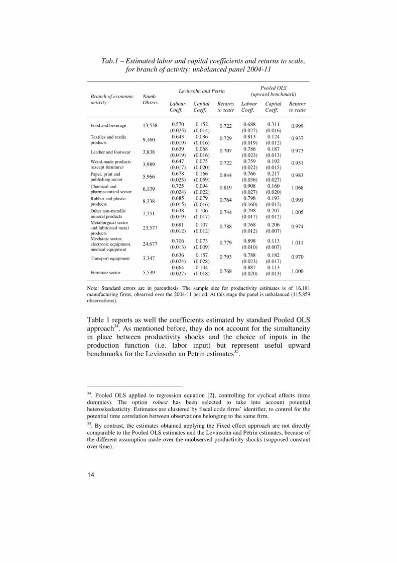
Tab.1 – Estimated labor and capital coefficients and returns to scale,

for branch of activity: unbalanced panel 2004-11

Branch of economic

activity

Numb.

Observ.

Levinsohn and Petrin

Pooled OLS

(upward benchmark)

Labour

Coeff.

Capital

Coeff.

Returns

to scale

Labour

Coeff.

Capital

Coeff.

Returns

to scale

Food and beverage 13,538 0.570

(0.025)

0.152

(0.014) 0.722 0.688

(0.027)

0.311

(0.016) 0.999

Textiles and textile

products 9,160

0.643

(0.019)

0.086

(0.016) 0.729 0.813

(0.019)

0.124

(0.012) 0.937

Leather and footwear 3,838 0.639

(0.019)

0.068

(0.016) 0.707 0.786

(0.023)

0.187

(0.013) 0.973

Wood-made products

(except furniture) 3,989

0.647

(0.017)

0.075

(0.020) 0.722 0.759

(0.022)

0.192

(0.015) 0.951

Paper, print and

publishing sector 5,966

0.678

(0.025)

0.166

(0.059) 0.844 0.766

(0.036)

0.217

(0.027) 0.983

Chemical and

pharmaceutical sector 6,139

0.725

(0.024)

0.094

(0.022) 0.819 0.908

(0.027)

0.160

(0.020) 1.068

Rubber and plastic

products 8,338

0.685

(0.015)

0.079

(0.016) 0.764 0.798

(0.160)

0.193

(0.012) 0.991

Other non-metallic

mineral products 7,751

0.638

(0.019)

0.106

(0.017) 0.744 0.798

(0.017)

0.207

(0.012) 1.005

Metallurgical sector

and fabricated metal

products 23,577

0.681

(0.012)

0.107

(0.012) 0.788 0.768

(0.012)

0.206

(0.007) 0.974

Mechanic sector,

electronic equipment,

medical equipment 24,677

0.706

(0.013)

0.073

(0.009) 0.779 0.898

(0.010)

0.113

(0.007) 1.011

Transport equipment 3,347 0.636

(0.024)

0.157

(0.028) 0.793 0.788

(0.023)

0.182

(0.017) 0.970

Furniture sector 5,539 0.664

(0.027)

0.104

(0.018) 0.768 0.887

(0.020)

0.113

(0.013) 1.000

Note: Standard errors are in parenthesis. The sample size for productivity estimates is of 16,181

manufacturing firms, observed over the 2004-11 period. At this stage the panel is unbalanced (115,859

observations).

Table 1 reports as well the coefficients estimated by standard Pooled OLS

approach34

. As mentioned before, they do not account for the simultaneity

in place between productivity shocks and the choice of inputs in the

production function (i.e. labor input) but represent useful upward

benchmarks for the Levinsohn an Petrin estimates35

.

34. Pooled OLS applied to regression equation [2], controlling for cyclical effects (time

dummies). The option robust has been selected to take into account potential

heteroskedasticity. Estimates are clustered by fiscal code firms’ identifier, to control for the

potential time correlation between observations belonging to the same firm.

35. By contrast, the estimates obtained applying the Fixed effect approach are not directly

comparable to the Pooled OLS estimates and the Levinsohn and Petrin estimates, because of

the different assumption made over the unobserved productivity shocks (supposed constant

over time).

15

Fig.1 – Total Factor Productivity (TFP) in the Italian manufacturing

industry: mean values 2004-11

4. The baseline model for productivity and innovation: exploiting the

features of a matched dataset between patent data and balance sheets

The estimated levels of firms’ total factor productivity were subsequently

applied as the reference dependent variable (in logarithms) into a baseline

model – without a spatial approach. The purpose was to shed light on

potential productivity advantages originating from a set of characteristics of

the operational context where firms are located.

At this purpose, the reference unbalanced panel for productivity

estimates was reduced into a balanced one of 8,803 geo-referenced

manufacturing firms, surveyed over the 2004-11 period as well. The

balancing of the original dataset, suitable to produce a considerable drop in

the number of available observations (70,424 observations were left, out of

the 115,859 observations in the unbalanced dataset for productivity

estimates), was desirable to prepare the ground for a further extension to a

spatial panel data approach.

16

From a dimensional point of view, a predominance of small firms is

detectable in the data: firms with less than 50 workers account for the

66,3% of the analyzed aggregate. Medium-size firms, with a number of

employees spanning from 50 to 249, present instead an incidence of 29,5%

and large firms, being those ones hiring more than 250 workers, account for

the remaining 4% of the panel dataset36

.

Following the strand of the literature on local productivity advantages,

we considered a panel data model of the form37

:

Log(tfp)it= β1mediumit +β2largeit+ β3innov_llsℓt*smallit +

+β4innov_llsℓt*mediumit +β5innov_llsℓt*largeit +

+β6innov_firmit +β7distrit +β8tecit +infrar +

+mt +mℓ +mv +εit [4]

Medium and large are binary variables describing the belonging of a

generic firm i in the specific year t to the subset of medium or large firms

described before (depending on the number of workers). They capture, as a

matter of fact, additional TFP premiums associated to medium and large

firms in the comparison to the baseline group, small firms in the sample.

The variables distrit and tecit capture instead the belonging to clusters of

firms with common specialization, identified here in the more traditional

sense: both the variables are dummy variables assuming value 1 if firms

belong to industrial districts (the 22% in the dataset) and technological

clusters (the 2% in the dataset) respectively. We exploit, at this purpose, the

definitions of the 144 industrial districts and the 22 technological clusters

monitored periodically by the Research Department of Intesa Sanpaolo:

industrial districts refer to firms’ agglomerations specialized in typical

“Made in Italy” productions (i.e. mechanical, textiles, food and beverage,

leather and footwear etc.) while technological clusters embed firms

specialized in the most “technological-based” activities (aerospace and

36. The subsample of deleted firms is made up of 7,377 subjects, with a composition in terms

of dimensional clusters similar to the one described so far for our balanced panel: small

firms account to represent the 67% of the sample, followed by medium and large firms, with

an incidence of 29% and around 3% respectively. This ensures that an almost random drop

of firms from the original dataset was performed. The only slightly higher percentage of

large firms remaining into our balanced panel (4%) is due to the higher probability of large

firms (with respect to the smallest ones) to remain in the Intesa Sanpaolo Integrated

Database for long time spans (i.e. to maintain a long banking relationship, such that their

balance sheets are present for recursive years in the dataset). By contrast, the percentage of

small firms removed from the original dataset (67%) is slightly higher with respect to the

one characterizing the balanced panel (around 66%).

37. A choice was made to exclude the constant from the model. We assume indeed that when

all the covariates of the model simultaneously assume a zero value, the dependent variable

(TFP) is zero as well.

17

aeronautical sectors, pharmaceutical sector, Ict)38

. It is worth stressing how

the definitions we account for in the present paper might encompass the

strategic proximity to urban areas, being also suitable to totally overlap to

them, in a few cases39

.

In order to (indirectly) identify the presence of potential knowledge

spillovers instead, suitable to generate important TFP premiums, we

constructed an index of the innovative activity attributable to the

operational space of firms in the panel. As already outlined in the previous

section, the presence of knowledge spillovers can be inferred indirectly,

through their impact on total factor productivity. Spillovers of these type

are mainly to be considered mixed spillovers, originating from market-

based exchanges. We exploited at this stage the features of a rich dataset on

patent data – patent applications registered at the European Patent Office

(EPO), referenced at the level of the applicant firm40

– matched to the

information on balance sheets that is present in the Intesa Sanpaolo

Integrated Database41

. To the best of our knowledge, the availability of

massive matched data on patents at the firm level is quite rare (in Italy a

similar dataset has been exploited so far only by the Bank of Italy42

).

Patent data represent, as a matter of fact, a high-quality proxy of

certified innovative output, the one subject to the lowest measurement

errors: they are directly attributable to realized and certified product

innovation at the firm level.

More precisely, we made use of patent data precisely localized on the

territory to build-up a sort of technological space for industrial activities.

We proceeded summing up demands for patents undersigned by

manufacturing firms43

at the level of broad territorial units, the ISTAT

Local labor systems (LLS)44

, for each sector of activity ℓ (3 digit, or 2 digit

38. For further details refer to the periodical reports “Industrial Districts Monitor” (quarterly)

and “Economics and Finance of Industrial Districts” (yearly) edited by Intesa Sanpaolo

SpA, Research Department.

39. There are no reason to retain “a priori” that industrial districts, being an agglomeration of

firms with a common specialization, are necessarily located far apart with respect to urban

centers and that those agglomeration economies are not in a position to benefit from the

advantages that being part of a urbanized area might offer.

40. In the (residual) cases of multiple applicant firms, decision was taken to consider a

multiple assignment of the same demand for patent.

41. The patent data come from the proprietary database Thomson Innovation, managed by

Thomson Reuters. The matching with data on balance sheets was performed – and is revised

on an annual basis according to new releases and/or revisions to the firm level data in the

Thomson Innovation dataset – by the Intesa Sanpaolo Research Department.

42. The dataset was exploited to estimate a model of innovation and trade that does not take

into account spatial features of firm productivity. Reference is made to the contribution of

Accetturo et al. (2014).

43. All the manufacturing firms associated to patent innovations available in the Intesa

Sanpaolo Integrated Database (around 4,800 firms) are considered.

44. Local labor systems are 784 territorial units identified by ISTAT (the Italian national

statistics institute) based on socio-economic relations. More precisely, they are a broad

18

sector from the Ateco 2007 classification for industrial activities,

depending on the available degree of detail in the matching process with

patents’ IPC codes – International patent classification codes45

). As

outlined before, LLS already proved to be a valid instrument to analyze the

socio-economic structure of the country. At this stage of the matching

process all the manufacturing firms associated to patent innovations

available in ISID were considered (around 4,800 firms) - and not merely

the geo-referenced firms present in our balanced panel (around 800 out of

the 4,800). The summation process of demands for patents, by sector ℓ and

LLS pair, was computed identical for each year t covered by our analysis –

that spans from 2004 to 2011. Moreover, in order to take into account the

potential time-lag occurring between a patent application at the EPO and

the moment of formal assignment of a patent to an applicant firm, we

proceeded summing up patent demands pertaining to a reference year

(pivotal year) t in the panel and to the previous four years - obtaining so far

a sort of rolling composite sum of patent applications. The variable

innov_llsℓt, being an index for relative patent intensity at the territorial

(LLS) level in the model (bounded between 0 and 100), was derived

dividing such a rolling composite sum - available at the sector ℓ /LLS pair –

for the same composite sum attributable to the ℓ-th specific manufacturing

sector at the national level46

:

������ℓ,,�� = ∑ ��������ℓ,��,������∑ ∑ ��������ℓ,��,������� ∗ 100

The variable was further assigned to firms in our balanced panel

according to their sector of activity ℓ, to the reference year t and to the LLS

they belong to. The mean value of the index is 2.7, suitable to identify a

codified innovative activity that is well spread across sectors and local

labour systems. As far as patent attitude of sectors is specifically

concerned, a traditional predominance of the electronic sector (with a mean

value of 19 demands for patents in the surveyed 2004-11 period), of the

pharmaceutical one (mean value of 15 demands), of the chemical sector

(mean value of 8 demands) and of the food sector (mean value of 5

demands) is detected.

aggregate of municipalities identified compacting information (drawn from the population

census survey) on daily trips of the resident population, for business purposes. The scope of

such a classification is to link municipalities showing consistent interdependence

relationships.

45. The matching process between IPC codes of patents and Ateco codes for industrial

activities, at the level of applicant firms, has been executed at the maximum degree of the

available breakdown (3 digits or 2 digits). The correspondence table between IPC codes and

Ateco is based on an updated version of the one present in Schmoch et al. (2003).

46. It is the aggregation of the demands for patents localized into all the Italian Local labor

systems, for a specific manufacturing sector (at 3 digit or 2 digit, depending on the

maximum degree of the available breakdown).

19

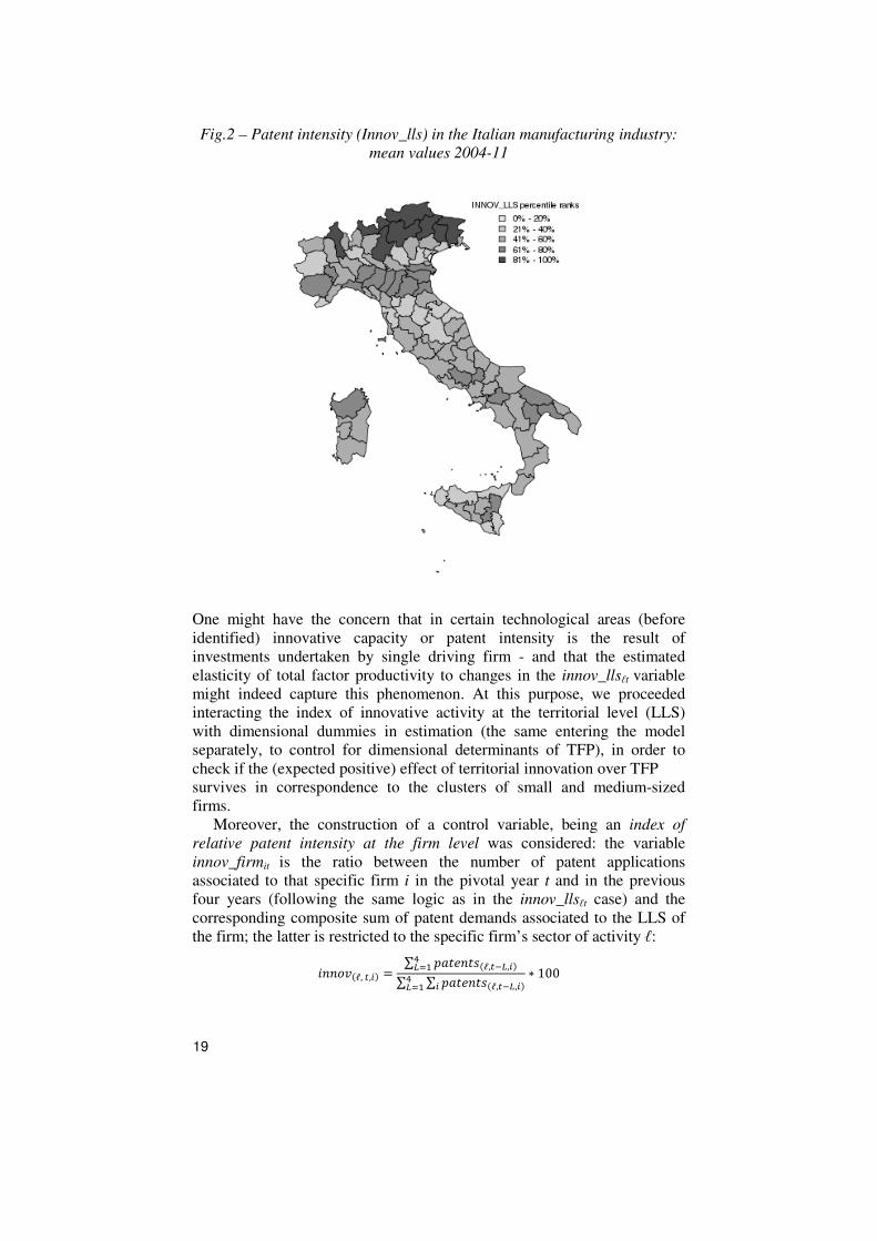
Fig.2 – Patent intensity (Innov_lls) in the Italian manufacturing industry:

mean values 2004-11

One might have the concern that in certain technological areas (before

identified) innovative capacity or patent intensity is the result of

investments undertaken by single driving firm - and that the estimated

elasticity of total factor productivity to changes in the innov_llsℓt variable

might indeed capture this phenomenon. At this purpose, we proceeded

interacting the index of innovative activity at the territorial level (LLS)

with dimensional dummies in estimation (the same entering the model

separately, to control for dimensional determinants of TFP), in order to

check if the (expected positive) effect of territorial innovation over TFP

survives in correspondence to the clusters of small and medium-sized

firms.

Moreover, the construction of a control variable, being an index of

relative patent intensity at the firm level was considered: the variable

innov_firmit is the ratio between the number of patent applications

associated to that specific firm i in the pivotal year t and in the previous

four years (following the same logic as in the innov_llsℓt case) and the

corresponding composite sum of patent demands associated to the LLS of

the firm; the latter is restricted to the specific firm’s sector of activity ℓ:

������ℓ,,�� = ∑ ��������ℓ,��,������∑ ∑ ��������ℓ,��,������� ∗ 100

20

The mean value of the index is 4.4 and the median is 0, because of the still

limited number of Italian manufacturing firms (the 9% in our panel - the

800 firms mentioned before) who gain access to a precise and codified

innovative activity (i.e. patenting).

In particular, the 3% of firms is associated one patent application and

the 2% two applications, corresponding indeed to the median value of

patent demands in the sample - while the mean value is around six

demands. In particular, the mean value of patent applications is two for the

cluster of small firms (that account to represent the 30% of the sample of

innovative firms), three for the cluster of medium firms (with an incidence

of around 49%) and 15 for the one of large firms (accounting for the

remaining 21%). Again, these evidences can be interpreted in favor of an

innovative activity that is well spread across firms belonging to a specific

LLS/sector pair and, in general, across the three broad dimensional clusters

in our dataset47

.

The error term in model [4] is a composite one; it is made up of four

components:

• a time-specific component mt accounting for business cycle

effects;

• an industry-specific component mℓ capturing sectorial

peculiarities of the TFP behavior;

• a territorial specific component mv accounting for territorial

peculiarities of the TFP phenomenon;

• an idiosyncratic error term εit.

The presence of time specific effects is accounted for introducing time

dummies (year dummies) in estimation, while sectorial dummies - at the

level of the branches of industrial activity exploited to estimate total factor

productivity - control for the presence of industry-specific effects. In order

to control for the presence of territorial peculiarities in measuring TFP

advantages, four categorical variables have been exploited, identifying the

belonging to broad macro-areas (North-East, North-West, South and

Islands, Center). Moreover, in addition to macro-geographical dummies,

the inclusion of an index proxying for the regional infrastructural

endowment was considered. At this purpose, we resorted to the indicators

of infrastructural development constructed by the Association of Italian

Chambers of Commerce (Unioncamere) in collaboration with the

“Guglielmo Tagliacarne” research institute48

. The index infrar (where the

subscript r stays for regions) allows to directly control for the effect of

47. The same checks have been executed over the subsample of firms drop from the original

unbalanced dataset for productivity estimates, in order to uncover the presence of potential

differences with respect to the balance dataset we have described so far. It is worth stressing

a mean value of 2.5 for the territorial index of innovative activity and a mean value of 4.2

for the index capturing the degree of innovative activity at the firm level.

48. The indicators were successfully employed in other works based on Italian data. See for

example the contribution from Minetti and Zhu (2011).

21

infrastructural development on firms’ total factor productivity and to

absorb (indirectly) potential spatial dependence in the data – the one

attributable to common features in the way to exploit territorial

infrastructures and institutions, that might differ considerably from one

region to the other.

Given the reduced time variability of the variables in our baseline model

(most of the regressors are time invariant), a panel estimation approach

with fixed effects does not represent an available option. By contrast, to

control for heterogeneity at the firm level (in addition to the before

mentioned sectorial and geographical dummies) we propose an estimation

framework based on random effects (RE). The representativeness of our

sample allows to reasonably consider the selected firms as randomly drawn

from a bigger population (random specific unobserved heterogeneity).

Preliminary estimates – that do not assume any spatial structure in the

data (column 1 in Tab.2)49

- highlight the presence of a strong link between

productivity, at the firm level and the patent intensity of the local labor

system where the firm is located, for what concerns its specific sector of

industrial specialization – captured by the variable innov_llsℓt. Even if firms

are not patenting directly, they might benefit from being located into a

patent intensive area. The result is suitable to support, at least indirectly,

the central role of innovation in enhancing total factor productivity. The

phenomenon is detectable in correspondence to all firms’ dimensional

clusters in the sample: it is worth stressing how a positive and strongly

significant elasticity of TFP to territorial innovation is uncovered with

reference to small firms (innov_lls*small). As mentioned before, the

inclusion of an index for relative patent intensity at the firm level within the

estimation framework (innov_firmit) ensures that the before results are not

merely driven by erroneous attribution to areas of spillover effects

pertaining to the innovative capacity of single larger firms.

Moreover, the inclusion in the model of a separate block of dimensional

dummies controls for the relevant effects of dimensions on total factor

productivity. Larger firms are traditionally associated “a priori” higher

levels of TFP.

Last but not least, consistently to the literature, a positive link is

established between total factor productivity and the belonging to clusters

of industrial subjects sharing a common specialization: positive elasticities

are in fact estimated in correspondence to dummies proxying for industrial

districts and technological clusters.

As already outlined in the introductive section, standard econometric

techniques are unable to account for important feedback loops arising from

the multidirectional nature of spatial dependence in the productivity

phenomenon: this is suitable to result into biased and inconsistent estimates

(endogeneity bias), as well as into spatially dependent residuals - like the

49. Estimates were performed through the R software (http://www.r-project.org/), plm

package (Linear models for panel data, Croissant and Millo).

22

ones plotted in Fig.3 – and a poorly predicted dependent variable (a

combined mix of underestimated and overestimated values of the variable

in space (Anselin and Le Gallo, 2006). In order to allow for a proper

estimation of the coefficient parameters, as well as for a proper

quantification of the spatial content of the productivity spillover, we move

to a formal spatial econometric framework.

Fig.3 – The plot of the residuals of the basic model, after non spatial

estimation (Panel Random Effect estimator)

5. A spatial approach to productivity: the role played by geographical

and sectorial distances between firms

Spatial econometrics comes to represent the econometric branch devoted to

formalize and measure spatial relationships in place between objects (i.e.

countries, regions or provinces at the macro level or firms at the micro

level)50

. In analyzing data pertaining to geographical entities, it is in fact

important to deal with spatial dependence, in addition to simple spatial

heterogeneity. The latter arises when diversified spatial units are employed

50. The contributions from Paelink and Klaasen (1979), Anselin (1988) and most recent ones

from Anselin and Le Gallo (2008), Le Sage and Pace (2009) are considered milestones in

the spatial econometrics field.

23

into the analysis and can be handled easily, resorting to standard

econometric techniques. Spatial dependence instead, or spatial

autocorrelation when the dependence is of the linear type, emerges when

realizations of the same variable are ordered according to a spatial

scheme51

. More precisely, it is hard detecting a unique causal direction for

connections established within a spatial context – differently from the time

series processes, where the causal direction goes from “past to future”

realizations of a variable: this renders standard econometric techniques

improper to quantify the importance of spatial relationships.

Spatial econometrics’ techniques are exactly designed to cope with this

“multi-directional feature” of spatial phenomena. Our attention will move

in particular towards the estimation of a spatial panel data model, with

random effects, exploiting at best the features of our data.

As a preliminary step, a global index of spatial autocorrelation of the

Moran’s I type was applied to our productivity data, to highlight the

importance of switching from a standard econometric approach to a spatial

one. The index is intended to detect the presence of correlation of the

spatial type: the more spatial objects (firms, in our case) are similar with

respect to the values undertaken by a certain variable under scrutiny

(productivity, our dependent variable in the model), the higher the value of

the index52

. It is nevertheless worth stressing that the Moran’s I index is

based on some restrictive assumptions53

: it is desirable to limit the

interpretation of results coming from the test to the detection of spatial

correlation in the data, leaving the assessment of its strength to a more

complex spatial econometric framework.

More precisely, we proceeded computing the Moran’s I index with

reference to our estimated (mean) TFP levels54

, the ones pertaining to the

51. Spatial autocorrelation can be defined as the relationship in place between pairs of

observations drawn from the same variable under scrutiny. The concept is implicit in the

broader one of spatial concentration of objects, i.e. the attitude of empirical phenomena to

assume similar values when close in space. More formally, spatial dependence means a

covariance different from zero between the values assumed by a variable in different

locations.

52. The values can vary between -1 (perfect dispersion) and +1 (perfect spatial correlation).

When dealing with micro-data it is reasonable to accept values of the index that fall in a

interval around zero: in the case of values of the index greater than zero, positive spatial

dependence is detected.

53. A simplifying assumption is the one of equality of variances between the value assumed

by a variable in one location i and the spatial lag of the same variable (based on the values

assumed in locations j). The test can in fact be considered an extension to the spatial case of

the Durbin Watson test applied to detect serial correlation in time series processes.

54. Choice was made to perform the test over mean TFP values (averaging over time) -

instead of switching to a pooled Moran’s I test option – to avoid computational issues and to

reduce the memory footprint. Indeed, due to the magnitude of the W matrix (8.803 x 8.803)

a pooled Moran I test would involve the construction of a pooled dense matrix of size (n*t)2

= 7.75e9. Considering a double value storage, this would imply a memory footprint of

approx. 58 GB, introducing heavy computational issues.

24

8,803 manufacturing firms of the balanced panel presented in Section 4. To

identify spatial relationships in place between testable objects, a basic W

matrix of reciprocal influences was constructed (whose role in the

estimation procedure will be detailed further and whose structure will be

subject to refinement in subsequent steps), based on their geographical

distance. At this purpose, firms were geo-referenced according to latitude

and longitude coordinates (Fig.4). The starting point was the location of the

municipality pertaining to the main operational headquarter of each firm in

the panel55

: geographical distances in kilometers dij (between a firms i and a

generic neighbor firm j) were computed accordingly, based on the great

circle method56

.

Fig.4 - The 8,803 geo-referenced Italian manufacturing firms present in

our balanced panel 2004-11

55. Choice was made to consider pluri-localized firms as uni-localized ones, based on the

coordinates attributed to the main operative headquarter of the firm. In light of the above, it

is possible to associate to each firm in the panel a univocally identified position and to build

up a unique matrix of distances W, of the order n x n, where n is the number of firms

considered in the analysis.

56. According to the great circle method, distances are measured in kilometers taking into

account the Earth curvature.

25

Based on the before mentioned “raw” W matrix, the performed Moran’s I

test for spatial correlation (under both normal approximation and

randomization assumptions) shows the presence of positive spatial

correlation in the data, with a highly robust significance (p-value < 2.2e-

16): the empirical value of the Moran's I statistic is 0.0520 (expected value

E[I] = -1/(N-1) = -0.0011 and variance V[I]=7.9685e-07).

These preliminary results encourage the adoption of a spatial approach

to properly estimate our productivity framework. If firm productivity levels

at location i depend on the levels observed in location j and vice-versa, the

data generating process becomes simultaneous: firms that are close in space

tend to display similar values of productivity, because of spillover effects.

Such a phenomenon is referred to as “clustering”57

.

More precisely the presence of a productivity spillover can be modeled,

as a first step, resorting to a spatial (random effect) panel model of the type

(in stacked form):

Log(tfp)t = λWlog(tfp)t + Xtβ + εt [5]

where the Log(tfp)t object contains levels of total factor productivity (of

a generic firm i at time t, in logs) estimated in Section 1, λ is the spatial

autoregressive parameter associated to the spatial lag of productivity

Wlog(tfp)t (the one accounting for weighted contributions of the

productivity levels pertaining to neighboring firms j), Xt is a vector of

exogenous covariates and εt is a pure idiosyncratic component. A spatial

model of this type, where a spatially lagged dependent variable is present,

is called Spatial autoregressive (SAR) of order one. Relationships in place

between spatial objects can be better visualized rewriting the linear model

in equation [5] as (substituting in Xt all the exogenous variables and

control variables already described in Section 3):

Log(tfp)it= λ ∑ ������� log(tfp)jt +β1mediumit +β2largeit +

+β3innov_llsℓt*smallit +β4innov_llsℓt*mediumit +

+β5innov_llsℓt*largeit +β6innov_firmit +β7distrit +

+β8tecit +infrar +mt +mj +mv +εit [6]

When the autoregressive parameter is greater than zero, the variable

under scrutiny (productivity) is positively autocorrelated in space and a

spillover effect is detected58

.

57. Clustering can be present in two different forms. In a true contagion framework leader

firms are assumed to locate randomly in the space while “followers” or subcontractors

display a positive probability to locate closeby. When instead exogenous conditions impose

the location of firms in certain areas (or certain areas display a higher probability to host

firms) a phenomenon of apparent contagion is in place. We will come back to this point

when discussing spatial dependence in the error term of our selected model.

58. When instead the autoregressive parameter is negative (λ<0) the variable under scrutiny

(productivity) is negatively autocorrelated in space: firms located closeby tend to display

different values (segregation).

26

The weighting scheme, the one suitable to model reciprocal influences

within the neighborhood, is contained into the W matrix. Therefore, it is

worth discussing in detail the construction of such an object, that is crucial

to correctly identify productivity spillovers: spatial econometrics estimates

are in fact particularly sensitive to the choice of W. The latter is a quadratic

matrix n x n (where n is again the number of firms in the sample, 8,803),

with zero diagonal elements59

. The generic elements wij are referred to as

“spatial weights”, measuring the strength of the relationship between a firm

i and a neighbor firm j.

W = ! 0 ⋯ w�$⋮ ⋱ ⋮w$� ⋯ 0 ' Different approaches can be accounted for to retrieve those coefficients.

The reference matrix in our analytical framework relies on geographical

influences exerted by first order neighboring firms60

. Influences are in turn

calculated relying on the dij distances mentioned before: more precisely,

spatial weights come to represent the reciprocal of the dij pairwise distances

in kilometers between firms in the dataset: wij=1/dij.

This way of modeling influences is not free from drawbacks. When

distances between firms are small, in fact, the elements wij of the matrix

tend to assume large values: limd→0 w=∞. In light of the above, it is

desirable to introduce some corrections. In primis, firms displaying

pairwise distances lower than 1 kilometer were assigned a unitary distance

(maximal reciprocal influence wij= 1).

Moreover, the structure of the W matrix was additionally refined,

exploiting results from the analysis of the Moran’s I index as a function of

pairwise distances. Upon construction of a correlogram (Fig.5) it is

possible to shed light on a clear pattern of decay in spatial correlation

between levels of TFP of Italian firms, as long as geographical distance

increases: correlation becomes close to zero when pairwise distances fall

within the range [300,400] Km.

59. The diagonal elements correspond to the influence exerted by a firm on itself.

60. It could be possible to define weights based on the interactions between neighbours of the

second order as well (neighbours of neighbours). But second order neighbours are, in their

turn, the first order neighbours of other spatial objects: this introduces simultaneous

interactions into the model, where each observation depends on the influence exerted by

both second order and first order neighbours. The influences λ of order greater than the first

one tend to decrease exponentially.

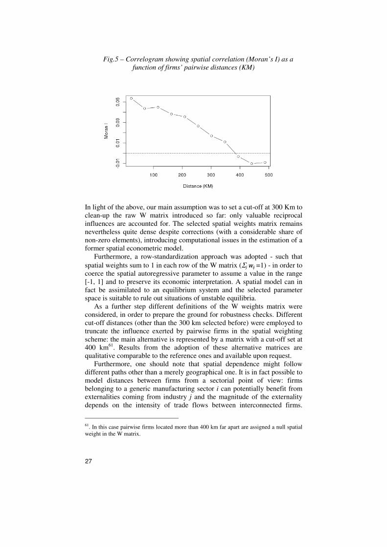
27

Fig.5 – Correlogram showing spatial correlation (Moran’s I) as a

function of firms’ pairwise distances (KM)

In light of the above, our main assumption was to set a cut-off at 300 Km to

clean-up the raw W matrix introduced so far: only valuable reciprocal

influences are accounted for. The selected spatial weights matrix remains

nevertheless quite dense despite corrections (with a considerable share of

non-zero elements), introducing computational issues in the estimation of a

former spatial econometric model.

Furthermore, a row-standardization approach was adopted - such that

spatial weights sum to 1 in each row of the W matrix (Σj wij =1) - in order to

coerce the spatial autoregressive parameter to assume a value in the range

[-1, 1] and to preserve its economic interpretation. A spatial model can in

fact be assimilated to an equilibrium system and the selected parameter

space is suitable to rule out situations of unstable equilibria.

As a further step different definitions of the W weights matrix were

considered, in order to prepare the ground for robustness checks. Different

cut-off distances (other than the 300 km selected before) were employed to

truncate the influence exerted by pairwise firms in the spatial weighting

scheme: the main alternative is represented by a matrix with a cut-off set at

400 km61

. Results from the adoption of these alternative matrices are

qualitative comparable to the reference ones and available upon request.

Furthermore, one should note that spatial dependence might follow

different paths other than a merely geographical one. It is in fact possible to

model distances between firms from a sectorial point of view: firms

belonging to a generic manufacturing sector i can potentially benefit from

externalities coming from industry j and the magnitude of the externality

depends on the intensity of trade flows between interconnected firms.

61. In this case pairwise firms located more than 400 km far apart are assigned a null spatial

weight in the W matrix.

28

Balance sheets do not report information concerning intra-firm trade but it

is reasonable to rely on sectorial proxies (Medda and Piga, 2007). ISTAT

input output matrices offer the right framework to disentangle the intensity

of trade connections in place between main sectors in the economy62

. In

order to model the effects of productivity spillovers from other industries

two additional matrices were constructed Wd (for demand-driven

spillovers) and Ws (for supply-driven spillovers). In the specific case of the

demand driven spillover matrix Wd, spatial weights wdij correspond to the

sales’ share of industry i to industry j or intermediate sales (how much of

the production of industry i is allocated to industry j63

), at 2 digit level

(Ateco 2007/Nace Rev.2 classification for industrial activities),

standardized by the total amount of sales assigned to the sector i in the

economy (the sum of intermediate sales and final sales), to control for its

relative importance. By contrast, spatial weights wdij in the supply driven

matrix Ws correspond to the purchases’ share of industry i from industry j,

properly standardized as well. Moreover, in order to preserve the same

economic interpretation for the spatial autoregressive parameter λ in the

model, sectorial-based spatial weights were further row-standardized.

From the point of view of an econometric estimation of model [6], it is

worth stressing the inconsistency and inefficiency of standard panel data

estimators (i.e. the random effect panel estimator adopted in section 4), not

accounting for the correlation in place between errors and the spatially

lagged dependent variable (endogeneity issue).

The maximum likelihood approach (Anselin, 1988) comes to represent

the “most popular”64

routine to consistently estimate the parameters of a

spatial model but results in turn to be hardly implementable on large

samples, like the one we are considering in the present paper (where the

spatial recursive system is based on a dense W weights matrix of order

8,803 x 8,803 and is extended to encompass a panel structure with a

temporal length of 8 years). In fact, when spatial dependence is detected in

the data and a spatially lagged dependent variable is considered to model it

directly (SAR model), the log-likelihood function is augmented for an

additional term depending on the autoregressive parameter λ (the Jacobian

or the log determinant of the (I-λW) matrix). That latter is going to

introduce computational difficulties in estimation: different from the time

series case, the Jacobian is not supposed to tend to zero as the sample size

increases. As a matter of fact, it constrains the autoregressive parameter

62. Specific reference is made to the ISTAT symmetric input output matrix of the “sector by

sector”62 type (release 2013 – the one corresponding to the release 2010 of the Italian

national accounts).

63. They represent, as a matter of fact, the inter-industrial intermediate flows between the

different sectors in the economy before the final product is made available on the

consumption or investment market. Sales from a generic sector i to sectors j can be red in

rows within the symmetric matrix.

64. The preferred choice in dealing with small finite samples.

29

values to their feasible range between the inverses of the smallest and

largest eigenvalues of the spatial weights matrix W 65

.

Moreover, computational issues are going to be exacerbated by a further

refinement of the spatial framework considered in our paper. With the

purpose to allow explicitly for spatial diffusion of disturbances in the

model, the error term in [5] was assigned an additional autoregressive

structure ρWut, where u is a composite error term (the sum of the AR(1)

term and the idiosyncratic term ε).

Once the new error equation is embedded into the SAR model, an

evolution of the basic model is achieved, the SARAR model (in stacked

form):

log(tfp)t = λWlog(tfp)t + Xtβ + ut

ut= ρWut +εt [7]

The W matrix in the error equation is assumed identical to the one in the

main equation.

The SARAR approach is justified by the presence of potential latent

variables correlated in space, not properly accounted for in the previous

specification of the model. While the spatial lag Wlog(tfp)t is suitable to

model direct spatial dependence in the data, the introduction of additional

structure into the error term can be indeed viewed as a way to model

indirect spatial dependence or, in other words, to model a dependence

coming from an external source. In particular, once an autoregressive

structure is considered (of order one, in our case), dependence in the error

term is potentially allowed to propagate without restrictions66

.

65. The simple SAR model y= λWy +Xβ +ε can be rewritten as (I-λW)y= Xβ +ε exploiting

matrix properties, with ε ∼ N(0, Iσ2). The parameter vector is Ө= (λ, β, σ2). For λ ≠0 the log

likelihood becomes:

ℓ(Ө) = − �) ln�2-� − �) ln�σ)� − �.�λ/0�12�3�.�λ/0�12�)σ4 + ln|7 − λW| The inclusion of the ln|7 − λW| term, that is referred to as the Jacobian, is suitable to

introduce computational problems in estimating spatial models with a consistent amount of

data (a spatial panel of 8,800 manufacturing firms surveyed over 8 years, in our specific

context), even when “saving time” or approximation procedures are adopted. The most

recurrent one is the “eigenvalues method” proposed to approximate the Jacobian. In fact,

unlike the time series case, the logarithm of the determinant of the (n x n) asymmetric matrix

(I - λW) does not tend to zero with increasing sample size: it constrains the autoregressive

parameter values to their feasible range between the inverses of the smallest and largest

eigenvalues of W – corresponding exactly to the range [-1,1] when the matrix is row-

standardized.

66. In fact, the error term AR(1) equation can be rewritten as:

ε= (I + ρW)-1u = u + ρWu + ρ2W2u + …

This expanded formula is suitable to show how spatial dependence is allowed to go far away

with respect to a Moving Average (MA) specification of the type u= ρWε +ε, where instead

dependence is much more restricted.

30

A battery of LM (Lagrange Multiplier) tests is reported here to justify the

adoption of the SARAR specification. In particular, a Conditional LM test

for λ (the autoregressive parameter of the spatially lagged dependent

variable) and a Conditional LM test for ρ (the autoregressive parameter of

the error term) were selected to properly evaluate the fit of the model.

While testing for the presence of a single type of spatial dependence in the

data (direct or indirect), these tests - extended by Baltagi et al. (2003) to the

case of spatial panel data models - prove to be robust to the simultaneous

presence of the other effect67

.

More precisely, a variant of the tests proposed by Baltagi et al. was

implemented in the paper, based on the residuals coming from a GM/IV

estimation of our spatial model (further details on the GM/IV routine will

follow)68

.

The conditional LM test for λ (assuming ρ≥0) reports a statistic of

4.6823, showing a highly significant spatial autocorrelation (p-value =

2.837e-06). The conditional LM test for ρ (assuming λ≥0) reports instead a

statistic of 192.9238, showing strong random spatial dependence (p-

value<2.2e-16). These results corroborate the previous choice for the model

structure.

To estimate a complete SARAR model, based on dense matrices and on

a large panel - like to one we introduced before, a switching to the Spatial

2SLS (Two Stage Least Squares) estimator proposed by Kapoor et al.

(2007) was considered, based on an ideal set of instruments for the

endogenous spatial lag variable69

. The Spatial 2SLS resorts in turn to a GM

approach to consistently estimate the autoregressive parameter ρ in the

error equation. From now on we will refer to this procedure as the GM/IV

routine. More precisely, the ideal estimation framework for ρ encompasses

the use of a complete list of optimally weighted70

sample moments, to

construct an expression for the “quadratic form in sample moments”, the

67. The variance of the statistic is properly adjusted to take into account the presence of the

other effect ( the one that is not the object of testing), resulting therefore in a more correct

inference.

68. The tests presented in Baltagi et al. (2003) and implemented within the splm R package

are instead based on the residuals from a maximum likelihood estimation of a spatial model.

69. The endogeneity of the spatially lagged dependent variable in a spatial model requires an

IV approach to be implemented. The ideal instrument for the spatial lag, in a generic spatial

SAC/SARAR model of the type y= Xβ +λWy +u, with u= ρWu +ε, is represented by its

expected value (conditional to the exogenous covariates of the model): E(Wy|X). The

expression can be rewritten as a linear combination of the type: E(Wy|X) = W E(y|X) = W

(I-λW)-1Xβ = W(I + λW + λ2W2 + …)Xβ = WXβ + W2X(λβ) + W3X(λ2β) +…

The ideal set of instruments H must contain at least the linearly independent columns of (X,

WX) such that H = [ X, WX, W2X, …]. The proposed 2SLS estimator is based on the

crucial assumption E(H’u)=0. See Kapoor et al. (2007) for further details.

70. In the GM theory the optimal weighting matrix, to be exploited within the expression for

the “quadratic form in sample moments”, is represented by the inverse of the variance

covariance matrix of the sample moments, at the true parameters values. Emphasis is given

to the sample moments estimated more precisely (the ones with the smallest variance).

31

core of the minimization problem in the GM theory71

. Nevertheless, to

account for situations where computational difficulties arise72

, a simplified

weighting scheme is considered in Kapoor et al. This is exactly the case of

our model. Moreover, it is worth stressing how the GM/IV multistep

procedure is suitable to bypass the problem of calculating the Jacobian in

the log-likelihood function (the most critical point in the maximum

likelihood estimation) and to relax as well the normal distributional

assumption on the disturbances (that is implicit in a maximum likelihood

framework73

).

The before mentioned procedure, with simplified weighting scheme, has

been implemented to consistently estimate the parameters of the SARAR

model proposed in equation [7]74

, exploiting different definitions of spatial

neighborhood – the ones implicitly contained in W (geographical-based or

sectorial-based neighborhood). We resort to a customized version of the

available GM/IV package in R software (spgm), rearranged to solve for

specific computational issues pertaining to the adoption of dense spatial

weights matrices75

.

6. Commenting on empirical estimates

Results from the GM/IV estimation of a Spatial Autoregressive model of

order one (SAR) and a complete SARAR model with additional AR(1)

spatially autoregressive disturbances - based on our balanced panel of

8,803 Italian manufacturing firms, surveyed over the 2004-11 period -

71. The GM estimator is exactly the minimizer of that expression and the one exploiting the

optimal weighting scheme described before is also the efficient one.

72. In fact, the asymptotic variance covariance matrix of the sample moments involve a

computational count of up to O(n3) and the computation of the matrix becomes difficult

when a huge amount of data is taken into account.

73. An hypothesis of independent and identically distributed innovations ε is instead

maintained, allowed to be heteroskedastic, and is crucial to derive the set of moment

conditions exploited in the GM framework.

74. To account for the simplified weighting scheme within the estimation procedure

implemented with R code, the option “weights” has been selected in the spgm function (GM

estimation of spatial panel data models) of the splm package (Spatial panel data models in

R, Millo and Piras).

75. The R package “splm” (Millo and Piras, 2012) was modified accordingly in order to deal

with dense matrices of distances, using the class “dgeMatrix” and the Lapack routine of the

package “Matrix” (Bates and Maechler, 2014). The routine allows for optimization of

linear algebra calculations and matrix operations in presence of dense numeric matrices.

Moreover, all the kronecker products involving the use of big dense spatial matrices W were

decomposed accordingly, thus reducing allocated memory. In some extreme cases (as the

one of a matrix exceeding 80 GB) matrices were stored as memory-mapped files, using the

infrastructure of the R packages “bigmemory” and “bigalgebra” (Kane, Emerson and

Weston, 2013).

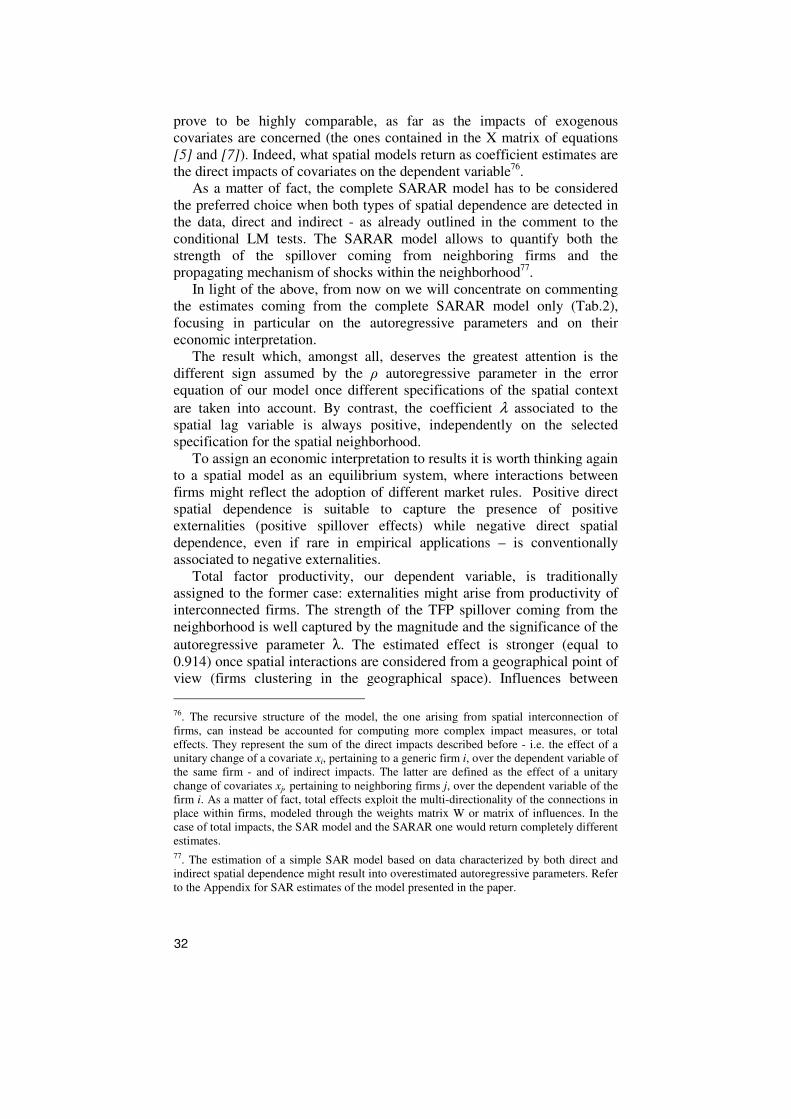
32

prove to be highly comparable, as far as the impacts of exogenous

covariates are concerned (the ones contained in the X matrix of equations

[5] and [7]). Indeed, what spatial models return as coefficient estimates are

the direct impacts of covariates on the dependent variable76

.

As a matter of fact, the complete SARAR model has to be considered

the preferred choice when both types of spatial dependence are detected in

the data, direct and indirect - as already outlined in the comment to the

conditional LM tests. The SARAR model allows to quantify both the

strength of the spillover coming from neighboring firms and the

propagating mechanism of shocks within the neighborhood77

.

In light of the above, from now on we will concentrate on commenting

the estimates coming from the complete SARAR model only (Tab.2),

focusing in particular on the autoregressive parameters and on their

economic interpretation.

The result which, amongst all, deserves the greatest attention is the

different sign assumed by the ρ autoregressive parameter in the error

equation of our model once different specifications of the spatial context

are taken into account. By contrast, the coefficient λ associated to the

spatial lag variable is always positive, independently on the selected

specification for the spatial neighborhood.

To assign an economic interpretation to results it is worth thinking again

to a spatial model as an equilibrium system, where interactions between

firms might reflect the adoption of different market rules. Positive direct

spatial dependence is suitable to capture the presence of positive

externalities (positive spillover effects) while negative direct spatial

dependence, even if rare in empirical applications – is conventionally

associated to negative externalities.

Total factor productivity, our dependent variable, is traditionally

assigned to the former case: externalities might arise from productivity of

interconnected firms. The strength of the TFP spillover coming from the

neighborhood is well captured by the magnitude and the significance of the

autoregressive parameter λ. The estimated effect is stronger (equal to

0.914) once spatial interactions are considered from a geographical point of

view (firms clustering in the geographical space). Influences between

76. The recursive structure of the model, the one arising from spatial interconnection of

firms, can instead be accounted for computing more complex impact measures, or total

effects. They represent the sum of the direct impacts described before - i.e. the effect of a

unitary change of a covariate xi, pertaining to a generic firm i, over the dependent variable of

the same firm - and of indirect impacts. The latter are defined as the effect of a unitary

change of covariates xj, pertaining to neighboring firms j, over the dependent variable of the

firm i. As a matter of fact, total effects exploit the multi-directionality of the connections in

place within firms, modeled through the weights matrix W or matrix of influences. In the

case of total impacts, the SAR model and the SARAR one would return completely different

estimates.

77. The estimation of a simple SAR model based on data characterized by both direct and

indirect spatial dependence might result into overestimated autoregressive parameters. Refer

to the Appendix for SAR estimates of the model presented in the paper.

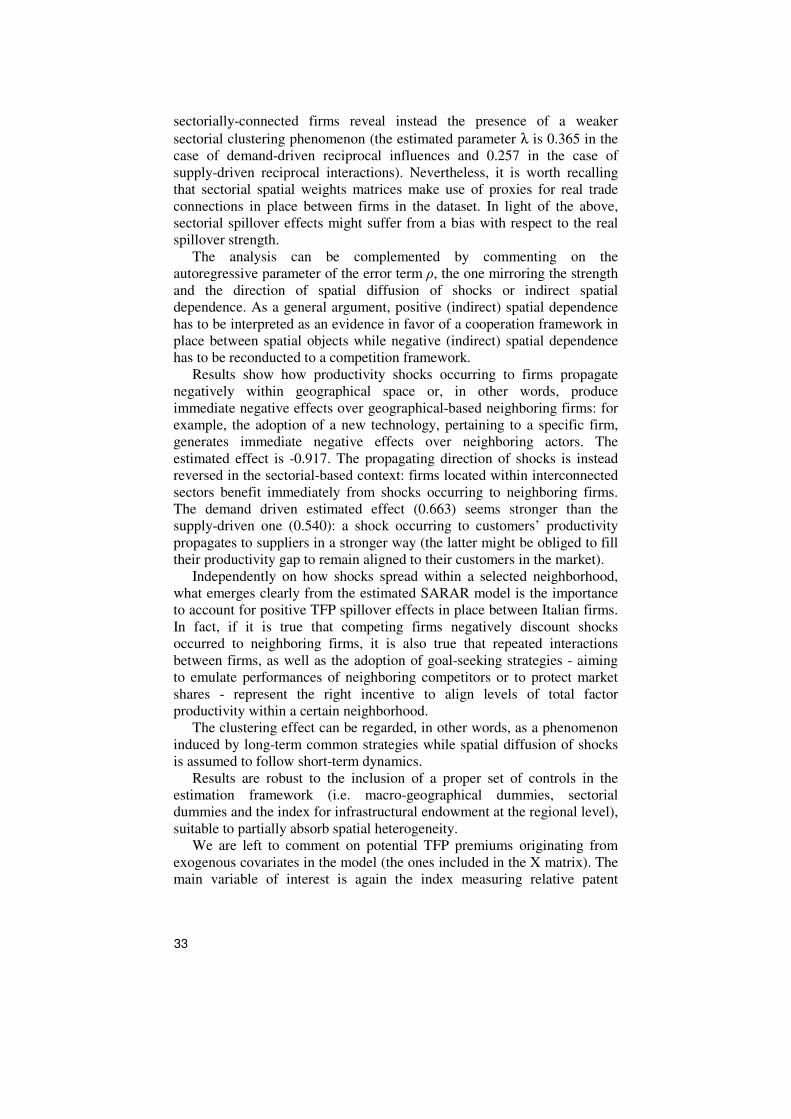
33

sectorially-connected firms reveal instead the presence of a weaker

sectorial clustering phenomenon (the estimated parameter λ is 0.365 in the

case of demand-driven reciprocal influences and 0.257 in the case of

supply-driven reciprocal interactions). Nevertheless, it is worth recalling

that sectorial spatial weights matrices make use of proxies for real trade

connections in place between firms in the dataset. In light of the above,

sectorial spillover effects might suffer from a bias with respect to the real

spillover strength.

The analysis can be complemented by commenting on the

autoregressive parameter of the error term ρ, the one mirroring the strength

and the direction of spatial diffusion of shocks or indirect spatial

dependence. As a general argument, positive (indirect) spatial dependence

has to be interpreted as an evidence in favor of a cooperation framework in

place between spatial objects while negative (indirect) spatial dependence

has to be reconducted to a competition framework.

Results show how productivity shocks occurring to firms propagate

negatively within geographical space or, in other words, produce

immediate negative effects over geographical-based neighboring firms: for

example, the adoption of a new technology, pertaining to a specific firm,

generates immediate negative effects over neighboring actors. The

estimated effect is -0.917. The propagating direction of shocks is instead

reversed in the sectorial-based context: firms located within interconnected

sectors benefit immediately from shocks occurring to neighboring firms.

The demand driven estimated effect (0.663) seems stronger than the

supply-driven one (0.540): a shock occurring to customers’ productivity

propagates to suppliers in a stronger way (the latter might be obliged to fill

their productivity gap to remain aligned to their customers in the market).

Independently on how shocks spread within a selected neighborhood,

what emerges clearly from the estimated SARAR model is the importance

to account for positive TFP spillover effects in place between Italian firms.

In fact, if it is true that competing firms negatively discount shocks

occurred to neighboring firms, it is also true that repeated interactions

between firms, as well as the adoption of goal-seeking strategies - aiming

to emulate performances of neighboring competitors or to protect market

shares - represent the right incentive to align levels of total factor

productivity within a certain neighborhood.

The clustering effect can be regarded, in other words, as a phenomenon

induced by long-term common strategies while spatial diffusion of shocks

is assumed to follow short-term dynamics.

Results are robust to the inclusion of a proper set of controls in the

estimation framework (i.e. macro-geographical dummies, sectorial

dummies and the index for infrastructural endowment at the regional level),

suitable to partially absorb spatial heterogeneity.

We are left to comment on potential TFP premiums originating from

exogenous covariates in the model (the ones included in the X matrix). The

main variable of interest is again the index measuring relative patent

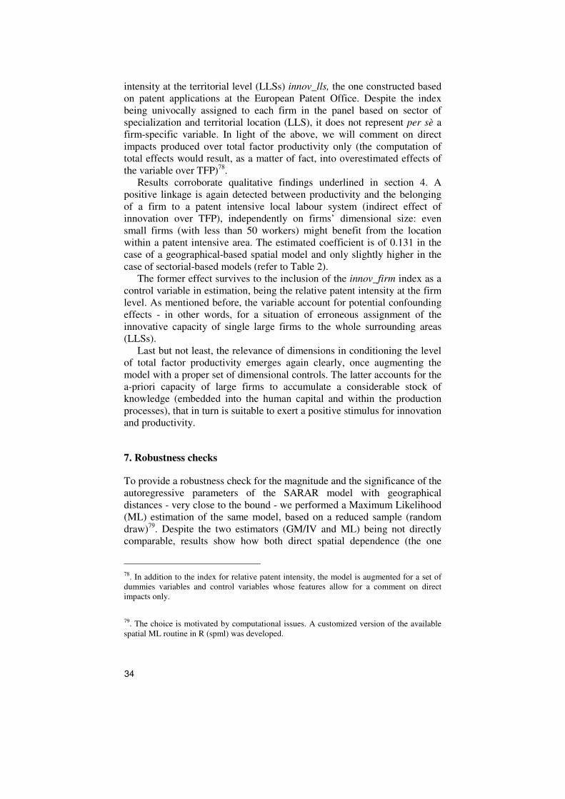
34

intensity at the territorial level (LLSs) innov_lls, the one constructed based

on patent applications at the European Patent Office. Despite the index

being univocally assigned to each firm in the panel based on sector of

specialization and territorial location (LLS), it does not represent per sè a

firm-specific variable. In light of the above, we will comment on direct

impacts produced over total factor productivity only (the computation of

total effects would result, as a matter of fact, into overestimated effects of

the variable over TFP)78

.

Results corroborate qualitative findings underlined in section 4. A

positive linkage is again detected between productivity and the belonging

of a firm to a patent intensive local labour system (indirect effect of

innovation over TFP), independently on firms’ dimensional size: even

small firms (with less than 50 workers) might benefit from the location

within a patent intensive area. The estimated coefficient is of 0.131 in the

case of a geographical-based spatial model and only slightly higher in the

case of sectorial-based models (refer to Table 2).

The former effect survives to the inclusion of the innov_firm index as a

control variable in estimation, being the relative patent intensity at the firm

level. As mentioned before, the variable account for potential confounding

effects - in other words, for a situation of erroneous assignment of the

innovative capacity of single large firms to the whole surrounding areas

(LLSs).

Last but not least, the relevance of dimensions in conditioning the level

of total factor productivity emerges again clearly, once augmenting the

model with a proper set of dimensional controls. The latter accounts for the

a-priori capacity of large firms to accumulate a considerable stock of

knowledge (embedded into the human capital and within the production

processes), that in turn is suitable to exert a positive stimulus for innovation

and productivity.

7. Robustness checks

To provide a robustness check for the magnitude and the significance of the

autoregressive parameters of the SARAR model with geographical

distances - very close to the bound - we performed a Maximum Likelihood

(ML) estimation of the same model, based on a reduced sample (random

draw)79

. Despite the two estimators (GM/IV and ML) being not directly

comparable, results show how both direct spatial dependence (the one

78. In addition to the index for relative patent intensity, the model is augmented for a set of

dummies variables and control variables whose features allow for a comment on direct

impacts only.

79. The choice is motivated by computational issues. A customized version of the available

spatial ML routine in R (spml) was developed.

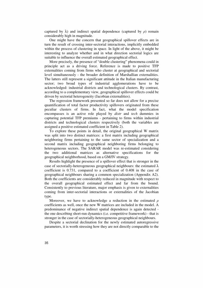
35

captured by λ) and indirect spatial dependence (captured by ρ) remain

considerably high in magnitude.

One might have the concern that geographical spillover effects are in

turn the result of crossing inter-sectorial interactions, implicitly embedded

within the process of clustering in space. In light of the above, it might be

interesting to analyze whether and in what direction sectorial logics are

suitable to influence the overall estimated geographical effect.

More precisely, the presence of “double clustering” phenomena could in

principle act as a driving force. Reference is made to positive TFP

externalities coming from firms who cluster at geographical and sectorial

level simultaneously - the broader definition of Marshallian externalities.

The latters still represent a significant attitude in the Italian manufacturing

sector; two broad types of industrial agglomerations have to be

acknowledged: industrial districts and technological clusters. By contrast,

according to a complementary view, geographical spillover effects could be

driven by sectorial heterogeneity (Jacobian externalities).

The regression framework presented so far does not allow for a precise

quantification of total factor productivity spillovers originated from these

peculiar clusters of firms. In fact, what the model specification

encompasses is an active role played by distr and tech dummies in

capturing potential TFP premiums - pertaining to firms within industrial

districts and technological clusters respectively (both the variables are

assigned a positive estimated coefficient in Table 2).

To explore these points in detail, the original geographical W matrix

was split into two distinct matrices: a first matrix including geographical

neighboring firms pertaining to the same sector of specialization and a

second matrix including geographical neighboring firms belonging to

heterogeneous sectors. The SARAR model was re-estimated considering

the two additional matrices as alternative specifications for the

geographical neighborhood, based on a GM/IV strategy.

Results highlight the presence of a spillover effect that is stronger in the

case of sectorially-heterogeneous geographical neighbours: the estimated λ

coefficient is 0.731, compared to a coefficient of 0.408 in the case of

geographical neighbours sharing a common specialization (Appendix A2).

Both the coefficients are considerably reduced in magnitude with respect to

the overall geographical estimated effect and far from the bound.

Consistently to previous literature, major emphasis is given to externalities

coming from inter-sectorial interactions or externalities of the Jacobian

type.

Moreover, we have to acknowledge a reduction in the estimated ρ

coefficients as well, once the new W matrices are included in the model. A

predominance of negative indirect spatial dependence is again detected -

the one describing short-run dynamics (i.e. competitive framework) - that is

stronger in the case of sectorially-heterogeneous geographical neighbours.

Despite a sectorial declination for the newly estimated autoregressive

parameters, it is worth stressing how they are not directly comparable to the

36

sectorial spillover effects estimated in the previous section. In the latter

cases in fact, sectorial space (proxied by trade) is considered to construct

pairwise interactions and modeled accordingly (input-output coefficients).

In the former cases instead, sectorial affiliations are exploited to further

refine the matrix of geographical interactions.

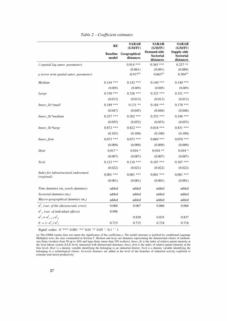
37

Table 2 – Coefficient estimates

RE SARAR

(GM/IV)

SARAR

(GM/IV)

SARAR

(GM/IV)

Baseline

model

Geographical

distances

Demand-side

Sectorial

distances

Supply-side

Sectorial

distances

λ (spatial lag autor. parameter)

0.914 *** 0.365 *** 0.257 **

(0.061) (0.091) (0.089)

ρ (error term spatial autor. parameter)

-0.917(a) 0.663(a) 0.504(a)

Medium 0.144 *** 0.142 *** 0.140 *** 0.140 ***

(0.005) (0.005) (0.005) (0.005)

Large 0.330 *** 0.326 *** 0.322 *** 0.321 ***

(0.013) (0.013) (0.013) (0.013)

Innov_lls*small 0.189 *** 0.131 ** 0.184 *** 0.178 ***

(0.047) (0.045) (0.046) (0.046)

Innov_lls*medium 0.257 *** 0.202 *** 0.252 *** 0.248 ***

(0.055) (0.052) (0.053) (0.053)

Innov_lls*large 0.872 *** 0.822 *** 0.818 *** 0.831 ***

(0.103) (0.100) (0.100) (0.100)

Innov_firm 0.073 *** 0.073 *** 0.069 *** 0.070 ***

(0.009) (0.009) (0.009) (0.009)

Distr 0.017 * 0.016 * 0.018 ** 0.018 *

(0.007) (0.007) (0.007) (0.007)

Tech 0.123 *** 0.118 *** 0.107 *** 0.107 ***

(0.022) (0.021) (0.022) (0.022)

Index for infrastructural endowment

(regional) 0.001 *** 0.001 *** 0.001 *** 0.001 ***

(0.001) (0.001) (0.001) (0.001)

Time dummies (mt, yearly dummies) added added added added

Sectorial dummies (mℓ) added added added added

Macro-geographical dummies (mv) added added added added

σ2ε (var. of the idiosyncratic error) 0.068 0.067 0.066 0.066

σ2 µ (var. of individual effects) 0.096

σ21 = σ2

ε + T σ2µ

0.830 0.835 0.837

θ = 1- σ2ε / σ

21 0.715 0.715 0.718 0.718

Signif. codes: 0 ‘***’ 0.001 ‘**’ 0.01 ‘*’ 0.05 ‘.’ 0.1 ‘ ’ 1

(a) The GMM routine does not report the significance of the coefficient ρ. The model structure is justified by conditional Lagrange Multiplier tests, the ones commented in Section 5. Medium and large are dummies representing the dimensional cluster of medium-

size firms (workers from 50 up to 249) and large firms (more than 250 workers); Innov_lls is the index of relative patent intensity at the local labour system (LLS) level, interacted with dimensional dummies; Innov_firm is the index of relative patent intensity at the

firm level; Distr is a dummy variable identifying the belonging to an industrial district; Tech is a dummy variable identifying the

belonging to a technological cluster. Sectorial dummies are added at the level of the branches of industrial activity exploited to

estimate total factor productivity.

38

Conclusions

The goal of the paper was to assess spillovers from total factor productivity

(TFP) in the Italian manufacturing industry, based on both geographical

and sectorial influences in place between firms and to disentangle the

effects of some core determinants of TFP premiums, innovation in primis.

We have provided concrete evidence of the importance to adopt a

spatial framework in dealing with series of data characterized by spatial

dependence, like productivity ones.

The concept of spillover effects from industrial clustering, still playing a

key role within the Italian industrial framework, can indeed be treated in a

more formal way while resorting to spatial econometrics techniques. More

precisely, exploiting a complete SARAR model we explicitly moved the

first steps towards a proper quantification of spillover effects from TFP and

tried to interpret propagation mechanisms of productivity shocks.

When geographical space is selected to define reciprocal interactions,

evidence was found of productivity shocks propagating in a negative way

within the neighborhood. By contrast, when attention is posed on sectorial

space, a positive propagating direction of shocks was detected. As a general

rule, positive indirect spatial dependence is suitable to identify the presence

of a cooperation framework and negative indirect spatial dependence of a

competition framework. Declining the argument towards our case, it is

feasible to think at geographical-based neighboring firms as competing

ones and to sectorial-based neighboring firms as cooperating ones.

Furthermore, the demand-driven sectorial estimated effect is stronger than

the supply-driven one: shocks occurring to customers’ productivity

propagates to suppliers in a stronger way.

The diffusion mechanism of shocks can indeed be assumed to mirror

short-run dynamics within a more general equilibrium system, like a spatial

econometric framework is. By contrast, the adoption of long-term common

strategies reflects into positive spillover effects. Significant evidence was

found of a positive spillover effect from total factor productivity of Italian

manufacturing firms. The effect is large in magnitude in the geographical

context (strong clustering phenomenon) while turning to be considerably

lower in the sectorial framework (weaker clustering phenomenon). Once

geographical spatial weights matrices are filtered according to sectorial

affiliation (common specialization versus sectorial heterogeneity), a

stronger geographical clustering effect is detected in correspondence to the

latter case – thus corroborating the findings of a primary role played by

Jacobian externalities.

The model presented in the paper contributed as well to the literature on

localized knowledge spillovers. We exploited the power of a measure of

relative innovative activity at the local labor systems’ (LLS) level, to detect

(at least indirectly) the presence of potential knowledge spillovers boosting

productivity. Firms located in patent intensive areas benefit from local

39

productivity premiums. The positive innovation effect is detectable in

correspondence to all firms’ dimensional clusters in the sample.

40

Appendix

A1. Branches of industrial activity

Branch Name

Ateco 2007/Nace

Rev.2 corresponding

codes

1 Food and beverage C.10, C.11

2 Textiles and textile products C.13, C.14

3 Leather and footwear C.15

4 Wood-made products (except furniture) C.16

5 Paper, print and publishing sector C.17, C.18

6 Chemical and pharmaceutical sector C.20, C.21

7 Rubber and plastic products C.22

8 Other non-metallic mineral products C.23

9 Metallurgical sector and fabricated metal products C.24, C.25

10 Mechanic sector, electronic equipment, medical

equipment C.26, C.27, C.28

11 Transport equipment C.29, C.30

12 Furniture sector C.31

41

A2. Robustness checks, SARAR model with geographical distances

SARAR (ML) SARAR (GM/IV) SARAR (GM/IV)

Geographical distances,

reduced sample

(random draw)

Geographical distances,

common sectorial

specialization

Geographical distances,

heterogeneous sectorial

specializations

λ (spatial lag autor. parameter) 0.905 *** 0.408 *** 0.731 ***

(0.001) (0.028) (0.060)

ρ (error term spatial autor.

parameter) -0.704 *** -0.580(a) -0.824(a)

(0.055)

Medium 0.112 *** 0.136 *** 0.143 ***

(0.008) (0.005) (0.005)

Large 0.328 *** 0.309 *** 0.328 ***

(0.019) (0.013) (0.013)

Innov_lls*small 0.149 * 0.157 * 0.160 *

(0.069) (0.042) (0.045)

Innov_lls*medium 0.296 *** 0.205 *** 0.231 ***

(0.079) (0.050) (0.053)

Innov_lls*large 0.580 *** 0.855 *** 0.845 ***

(0.148) (0.098) (0.100)

Innov_firm 0.066 *** 0.068 *** 0.073 ***

(0.013) (0.008) (0.009)

Distr 0.019 0.019** 0.015

(0.011) (0.006) (0.007)

Tech 0.122 *** 0.085 *** 0.119 ***

(0.030) (0.018) (0.021)

Index for infrastructural

endowment (regional) 0.001 *** 0.001 *** 0.001 ***

(0.001) (0.001) (0.001)

Time dummies (mt) added added added

Sectorial dummies (mℓ) added added added

Macro-geographical dummies (mv) added added added

φ = σ2µ / σ

2ε 1.743 ***

(0.049)

σ2ε (var. of the idiosyncratic error) 0.064 0.067

σ21 = σ2

ε + T σ2µ 0.847 0.832

θ = 1- σ2ε / σ

21 0.724 0.715

Signif. codes: 0 ‘***’ 0.001 ‘**’ 0.01 ‘*’ 0.05 ‘.’ 0.1 ‘ ’ 1

(a) The GMM routine does not report the significance of the coefficient ρ. The model structure is justified by conditional Lagrange

Multiplier tests, the ones commented in Section 5.

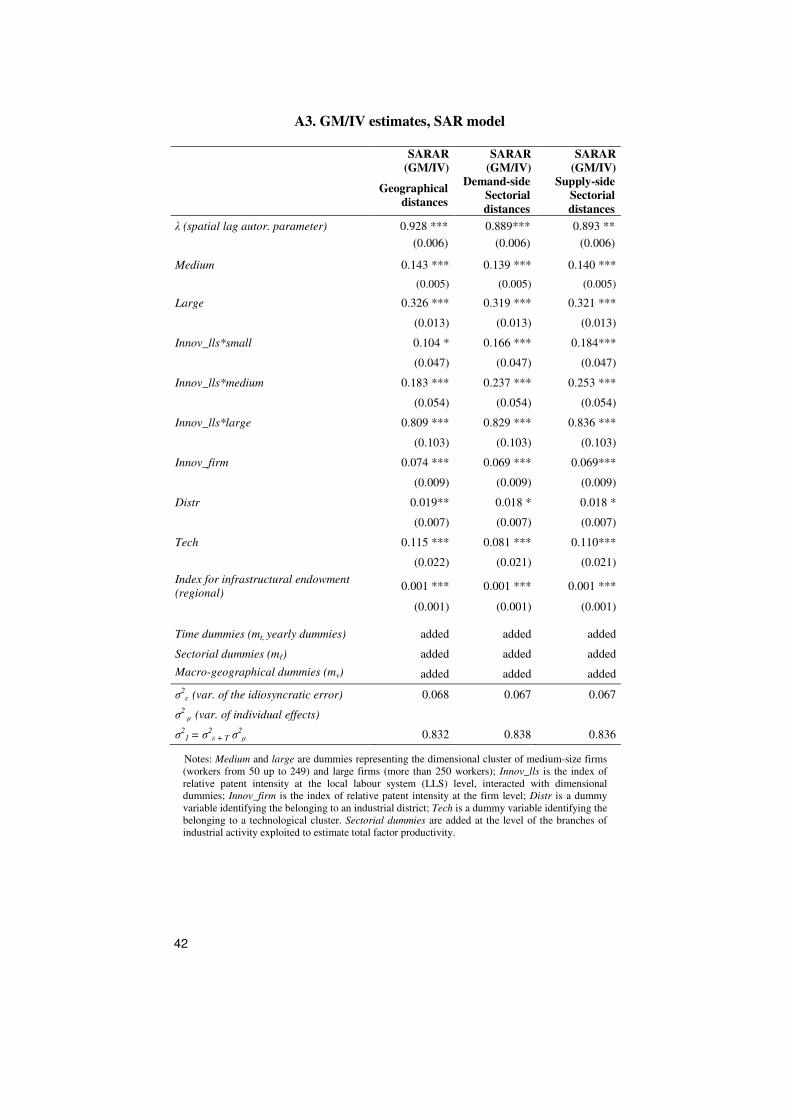
42

A3. GM/IV estimates, SAR model

SARAR

(GM/IV)

SARAR

(GM/IV)

SARAR

(GM/IV)

Geographical

distances

Demand-side

Sectorial

distances

Supply-side

Sectorial

distances

λ (spatial lag autor. parameter) 0.928 *** 0.889*** 0.893 **

(0.006) (0.006) (0.006)

Medium 0.143 *** 0.139 *** 0.140 ***

(0.005) (0.005) (0.005)

Large 0.326 *** 0.319 *** 0.321 ***

(0.013) (0.013) (0.013)

Innov_lls*small 0.104 * 0.166 *** 0.184***

(0.047) (0.047) (0.047)

Innov_lls*medium 0.183 *** 0.237 *** 0.253 ***

(0.054) (0.054) (0.054)

Innov_lls*large 0.809 *** 0.829 *** 0.836 ***

(0.103) (0.103) (0.103)

Innov_firm 0.074 *** 0.069 *** 0.069***

(0.009) (0.009) (0.009)

Distr 0.019** 0.018 * 0.018 *

(0.007) (0.007) (0.007)

Tech 0.115 *** 0.081 *** 0.110***

(0.022) (0.021) (0.021)

Index for infrastructural endowment

(regional) 0.001 *** 0.001 *** 0.001 ***

(0.001) (0.001) (0.001)

Time dummies (mt, yearly dummies) added added added

Sectorial dummies (mℓ) added added added

Macro-geographical dummies (mv) added added added

σ2ε (var. of the idiosyncratic error) 0.068 0.067 0.067

σ2 µ (var. of individual effects)

σ21 = σ2

ε + T σ2µ 0.832 0.838 0.836

Notes: Medium and large are dummies representing the dimensional cluster of medium-size firms

(workers from 50 up to 249) and large firms (more than 250 workers); Innov_lls is the index of

relative patent intensity at the local labour system (LLS) level, interacted with dimensional

dummies; Innov_firm is the index of relative patent intensity at the firm level; Distr is a dummy

variable identifying the belonging to an industrial district; Tech is a dummy variable identifying the

belonging to a technological cluster. Sectorial dummies are added at the level of the branches of

industrial activity exploited to estimate total factor productivity.

43

References

Accetturo A., Bugamelli M., Lamorgese A.R., Linarello A. 2014. Innovation and

trade. Evidence from Italian manufacturing firms. Temi di discussione della

Banca d’Italia 464.

Accetturo A., Di Giacinto V., Micucci G., Pagnini M. 2013. Geography,

productivity and trade: does selection explain why some locations are more

productive than others? Temi di discussione della Banca d’Italia 910.

Acs Z.J., Audretsch D.B., Feldman M. 1994. R&D spillovers and recipient firm

size. Review of Economics and Statistics, 76 (2) 336-340.

Agrawal A.K., Cockburn I.M., McHale J. 2003. Gone but not forgotten: labor

flows, knowledge spillovers, and enduring social capital. NBER Working Paper

9950.

Aiello F., Pupo V., Ricotta F. 2008. Sulla dinamica della produttività totale dei

fattori in Italia. Un’analisi settoriale. Università della Calabria Working Papers

03-2008.

Aitken, B., Harrison A. 1999. Do domestic firms benefit from foreign investment?

Evidence from Venezuela. American Economic Review, 89: 605-618.

Allegra E., Fiorini M., Grillo M., Magnani L. 2004. Antitrust policy and national

growth: some evidence from Italy. Giornale degli Economisti e Annali di

Economia, 63 (1): 69-86.

Anselin L., 1988, Spatial Econometrics: Methods and Models, Kluwer, Boston.

Anselin L., Le Gallo J. 2006. Interpolation of air quality measures in hedonic

house price models: spatial aspects. Spatial Economic Analysis, 1 (1): 31-52.

Audretsch D.B., Feldman M. 1996. Knowledge spillovers and the geography of

innovation and production. American Economic Review, 86 (3): 630-640.

Audretsch D.B., Feldman M. 1999. Innovation in cities: science-based diversity,

specialization and localized competition. European Economic Review, 43 (2):

409-429.

Autant-Bernard C. 2011. Spatial econometrics of innovation: recent contributions

and research perspectives. Working papers GATE (Groupe d’analyse et de

thèorie économique Lyon-St Etienne.

Baltagi B.H. 2013. Econometric analysis of panel data. 5th

edition. John Wiley &

Sons, New York.

Baltagi B.H., Song S.H., Koh W. 2003. Testing panel data regression models with

spatial error correlation. Journal of econometrics, 117: 123-150.

Bassanetti A., Iommi M., Jona-Lasinio C., Zollino F. 2004. La crescita

dell’economia italiana negli anni novanta tra ritardo tecnologico e

rallentamento della produttività. Temi di discussione della Banca d’Italia 539.

Bates D. and Maechler M. (2014) “Matrix: Sparse and Dense Matrix Classes and

Methods”

Becattini G. 1990. The Marshallian industrial district as a socio-economic notion.

in Pyke F., Becattini G., Sengenberger W. (eds.), Industrial Districts and Inter-

firm Co-operation in Italy, Geneva: International Labor Office: 37- 51.

Bera A. K., Florax, R., Yoon, M. J. 1996. Simple diagnostic tests for spatial

dependence. Regional Science and Urban Economics, 26: 77–104.

Bivand R.S., Pebesma E.J., Gomez-Rubio V. 2008. Applied Spatial Data Analysis

with R, Springer.

Brandolini A., Bugamelli M. 2009. Rapporto sulle tendenze nel sistema produttivo

italiano. Questioni di Economia e Finanza Banca d’Italia 45.

Brandolini A., Cipollone P. 2001. Multifactor productivity and labor quality in

Italy, 1981-2000. Temi di Discussione della Banca d’Italia 422.

44

Branstetter, L. 2001a. Are knowledge spillovers international or intranational in

scope? Microeconometric evidence from Japan and the United States. Journal

of International Economics, 53: 53-79.

Breschi S., Lissoni F. 2001. Cross-firm inventors and social networks: localized

knowledge spillovers revisited. Annales d’Economie et de la Statistique, 79-80:

189-209.

Breschi S., Lissoni F. 2005. Mobility and social networks: localized knowledge

spillovers revisited. Annales d’Economie et de Statistique , 79/80: 189-20

Breschi S., Lissoni F., Montobbio F. 2004. The geography of knowledge

spillovers: conceptual issues and measurement problems, in Breschi S.,

Malerba F. (ed) (2005), Clusters, Networks and Innovation. Oxford University

Press.

Breschi S., Malerba F. 2001. Geography of innovation and economic clustering.

Industrial and Corporate Change, 10 (4): 817-833.

Bronzini R., Piselli P. 2006. Determinants of long-run regional productivity: the

role of R&D, human capital and public infrastructure. Temi di Discussione

della Banca d’Italia 597.

Buccellato T., Santoni G. 2012. Produttività totale dei fattori (TFP) delle imprese

italiane: uno studio su distretti, aree urbane ed esternalità geografiche.

Fondazione Manlio Masi.

Bugamelli M., Rosolia A. 2006. Produttività e concorrenza estera. Temi di

Discussione della Banca d’Italia 578.

Buganza T., Bandoni P., Verganti R. 2007. Le relazioni tra impresa e università nel

paradigma dell’open innovation. Impresa & Stato, Franco Angeli, Milano, 78:

9-16.

Cainelli G., De Liso N. 2005. Innovation in Industrial Districts: Evidence from

Italy. Industry and Innovation, 12 (3): 383-398.

Carboni O.A. 2012. A spatial analysis of R&D: the role of industry proximity.

Working Paper, CRENoS 2012_04

Casaburi L., Minerva A., Gattai V. 2008. Firms international status and

heterogeneity in performance: evidence from Italy. Nota di Lavoro, 3.

Cingano F., Schivardi F. 2004. Identifying the Sources of Local Productivity

Growth. Journal of the European Economic Association, 2: 720-742.

Ciocca P. 2004. L’economia italiana: un problema di crescita. Rivista Italiana

degli Economisti, 9 (Supplemento al n.1): 7-28.

Colombo M.G., D’Adda D., Piva E. 2009. The contribution of university research

to the growth of academic start-ups: an empirical analysis. The Journal of

Technology Transfer.

Combes P., Duranton G., Gobillon L., Puga D., Roux S. 2012. The productivity

advantages of large cities: Distinguishing agglomeration from firm selection.

Econometrica, 80: 2543-2594 .

Confindustria. 2006. Produttività e attrattività del paese: i nodi da sciogliere.

Quaderni di Ricerca di Confindustria 2.

Corò G., Grandinetti R. 1999. Strategie di delocalizzazione e processi evolutivi

nei distretti industriali italiani. L’industria, 4.

D’Ignazio A., Menon C. 2013. The causal effect of credit guarantees for SMEs:

evidence from Italy. Discussion paper 900-13, Bank of Italy.

Daveri F. 2006. Perché la competitività ha smesso di crescere nell’economia

italiana?. Quaderni di Ricerca di Confindustria 2.

Daveri F., Jona-Lasinio C. 2005. Italy’s decline: getting the facts right. Giornale

degli Economisti e Annali di Economia, 64 (4): 365-410.

45

Dettori B., Maroccu E., Paci R. 2008. Total factor productivity, intangible assets

and spatial dependence in the European regions. CRENOS Working Papers 23.

Di Giacinto V., Gomellini M., Micucci G., Pagnini M. 2011. Mapping local

productivity advantages in Italy: industrial districts, cities or both?. Temi di

Discussione della Banca d’Italia 850.

Duranton G., Puga D. 2004. Microfoundations of urban agglomeration economies.

Within Henderson V., Thisse J.F. (eds.) Handbook of Regional and Urban

Economics, Amsterdam, NorthHolland, 4: 2063-2117.

Elhorst J.P. 2009. Specification and estimation of spatial panel data models.

International Regional Sciences Review, 26(3): 244-268.

Fabiani S., Pellegrini G., Romagnano E., Signorini L.F. 2000. Efficiency and

localization: the case of Italian districts, in Bagella M., Becchetti L. (eds.), The

Competitive Advantage of Industrial Districts: Theoretical and Empirical

Analysis, Heidelberg: Phisica-Verlag.

Fachin S., Gavosto A. 2007. The decline in Italian productivity: a study in

estimation of long-run trends in total factor productivity with panel

cointegration methods. MPRA Papers 3112.

Faini R., Sapir A. 2005. Un modello obsoleto? Crescita e specializzazione

dell’economia italiana, in Boeri T., Faini R., Ichino A., Pisauro G., Scarpa C. (a

cura di) Oltre il declino. il Mulino: Bologna.

Fantino D., Mori A., Scalise D. 2012. Collaboration between firms and universities

in Italy: the role of a firm’s proximity to top-rated departments. Temi di

Discussione Banca d’Italia 884.

Griliches Z. 1979. Issues in assessing the contribution of research and development

to productivity growth. Bell Journal of Economics, 10 (1): 92-116.

Griliches Z. 1992. The search for R&D spillovers. Scandinavian Journal of

Economics, 94: 29-47.

Haskel, J., Pereira S., Slaughter M. 2002. Does inward foreign direct investment

boost the productivity of domestic firms? NBER Working Paper 8724.

ISAE. 2005. Crescita e struttura produttiva dell’Italia: un confronto con i

principali paesi industriali. ISAE: Roma.

Iuzzolino G. 2008. Segnali di discontinuità nell’economia dei distretti: evidenze

statistiche dopo il 2001. AIP (Associazione Italiana delle Produzione) Reti di

imprese oltre i distretti Il Sole 24 Ore, Milano.

Iuzzolino G., Menon C. 2010. Le agglomerazioni industriali del Nord Est: segnali

di discontinuità negli anni duemila. Mimeo.

Iuzzolino G., Micucci G. 2011. Le recenti trasformazioni dei distretti industriali

italiani. Secondo Rapporto Nazionale dell’Osservatorio sui Distretti,

Federazione dei Distretti Italiani,Venezia.

Jacobs J. 1969. The Economy of Cities, New York: Random House.

Jaffe A. 1989. Real effects of academic research. American Economic Review, 79

(5): 957-970.

Jaffe A., Trajtenberg M., Henderson R. 1993. Geographic localization of

knowledge spillovers as evidenced by patent citations. Quarterly Journal of

Economics, 108 (3): 577-598.

Javorick B.S. 2004. Does foreign direct investment increase the productivity of

domestic firms? In search of spillovers through backward linkages. American

Economic Review, 94(3): 605-627.

Michael J. Kane, John Emerson, Stephen Weston (2013). Scalable Strategies for

Computing with Massive Data. Journal of Statistical Software, 55(14), 1-19.

46

Minetti R., Zhu S.C. (2011). Credit constraints and firm export: Microeconomic

evidence from Italy. Journal of International Economics, 83(11), 109-125.

Kapoor M., Kelejian H.H., Prucha I.R. 2007. Panel data model with spatially

correlated error components. Journal of Econometrics, 140(1): 97-130

Kelejian H.H., Prucha I.R. 1999. A generalized moments estimator for the

autoregressive parameter in a spatial model. International Economic Review,

40(2): 509-533.

Le Sage J., Pace R.K., 2009, Introduction to Spatial Econometrics, CRC Press.

Lee L-f., Yu J. 2010. Some recent developments in spatial panel data models.

Regional Science and Urban Economics, 40 (5): 255-271.

Levinsohn J., Petrin A. 2003. Estimating production functions using inputs to

control for unobservables. Review of Economic Studies, 70 (2): 317-341.

Malerba F., Montobbio F. 2003. Exploring factors affecting international

technological specialization: the role of knowledge flows and the structure of

innovative activity. Journal of Evolutionary Economics, 13 (4): 411-434.

Malerba F., Mancusi M., Montobbio F. 2003. Innovation and knowledge

spillovers: evidence from European data. Working Paper n. 39. University of

Insubria (prepared for the American Economic Association meeting, San Diego

January 5th

, 2003).

Marrocu E., Paci R., Usai S. 2010. Productivity growth in the old and new Europe:

the role of agglomerations externalities. CRENOS Working Papers 24/2010.

Marrocu E., Paci R., Usai S. 2011. The complementary effects of proximity

dimensions on knowledge spillovers. CRENOS Working Papers 21/2011.

Marshall A. 1890. Principles of Economics. London: Macmillan.

Medda G., Piga C. A., 2007. Technological Spillovers and Productivity in Italian

Manufacturing Firms. WP 2007-17 Loughborough University.

Milana C., Zeli A. 2003. Productivity slowdown and the role of ICT in Italy: a

firm-level analysis. ISAE Working Papers 39.

Millo G., Piras G. 2012. Splm: Spatial Panel Data Models in R. Journal of

Statistical Software, 47 (1)

Moran P. A. P. 1950, Notes on Continuous Stochastic Phenomena. Biometrika, 37:

17–33.

Moreno R., Paci R., Usai S. 2005. Spatial spillovers and innovation activity in

European regions. Environment and Planning, 37: 1793-1812.

Mowery D., Ziedonis A. 2001. The geographic reach of market and non-market

channels of technology transfer: comparing citations and licenses of university

patents. NBER Working Paper 8568.

Murat M., Paba S. 2005. I distretti industriali tra globalizzazione riorganizzazione.

AAVV Cambiamenti produttivi e politiche per lo sviluppo locale nell’Italia

mediana.

Nicoletti G., Scarpetta S. 2003. Regulation, productivity and growth: OECD

evidence. OECD Economics Department Working Papers 347.

Olley S., Pakes A. 1996. The dynamics of productivity in the telecommunications

equipment industry. Econometrica, 64 (6): 1263-1297.

Ord J. 1975. Estimation methods for models of spatial interaction. Journal of the

American Statistical Association, 70: 120–126.

Paci S., Usai R. 2000. The role of specialization and diversity externalities in the

agglomeration of innovative activities. Rivista Italiana degli Economisti, 5 (2):

237-268.

Paci S., Usai R. 2005. Agglomeration economies and growth. The case of Italian

local labour systems, 1991-2001. Working Paper, CRENoS 214.

47

Paelinck J.,Klaassen L.H. 1979. Spatial Econometrics, Saxon House, Farnbor

ough, 1979.

Peri G. 2003. Knowledge flows, R&D externalities and innovation. ZEW

Discussion Paper, 40 (3).

Piergiovanni R., Santarelli E., Vivarelli M. 1997. From which source do small

firms derive their innovative inputs? Some evidence from Italian industry.

Review of Industrial Organization, 12: 243-58.

Piergiovanni R., Santarelli E., Vivarelli M. 1997. From which source do small

firms derive their innovative inputs? Some evidence from Italian industry.

Review of Industrial Organization, 12: 243-58.

Pietrabissa R. e Conti G. 2005. Strategia per un rapporto responsabile fra ricerca

pubblica e industria. L’industria, 26 (3): 419-44

Piras G. (2010). sphet: Spatial Models with Heteroskedastic Innovations in R.

Journal of Statistical Software, 35(1), 1-21.

Romer P.M. 1990. Endogenous technological change. Journal of Political

Economy, 98 (5): 71-102.

Schmoch U., Laville F., Patel P., Frietsch R. 2003. Linking technology areas to

industrial sectors. Final Report to the European Commission, DG Research.

Signorini L.F. 1994. The price of Prato, or measuring the industrial district effect.

Papers in Regional Science, 73 (4): 369-392.

Thompson P., Fox-Kean M. 2005. Patent citations and the geography of

knowledge spillovers: a reassessment. American Economic Review, 95 (1):

450-460.

Venturini F. 2004. The determinants of Italian slowdown: what do the data say?.

EPKE Working Papers 29.