Embed Size (px)
Citation preview
sid.inpe.br/mtc-m21c/2020/05.27.18.15-TDI
A SPATIO-TEMPORAL BAYESIAN NETWORKMODEL: A CASE STUDY IN BRAZILIAN AMAZON
DEFORESTATION PREDICTION
Alexsandro Cândido de Oliveira Silva
Doctorate Thesis of the GraduateCourse in Applied Computing,guided by Dra. Leila Maria GarciaFonseca, approved in May 4, 2020.
URL of the original document:<http://urlib.net/8JMKD3MGP3W34R/42J382B>
INPESão José dos Campos
2020
PUBLISHED BY:
Instituto Nacional de Pesquisas Espaciais - INPEGabinete do Diretor (GBDIR)Serviço de Informação e Documentação (SESID)CEP 12.227-010São José dos Campos - SP - BrasilTel.:(012) 3208-6923/7348E-mail: [email protected]
BOARD OF PUBLISHING AND PRESERVATION OF INPEINTELLECTUAL PRODUCTION - CEPPII (PORTARIA No
176/2018/SEI-INPE):Chairperson:Dra. Marley Cavalcante de Lima Moscati - Centro de Previsão de Tempo e EstudosClimáticos (CGCPT)Members:Dra. Carina Barros Mello - Coordenação de Laboratórios Associados (COCTE)Dr. Alisson Dal Lago - Coordenação-Geral de Ciências Espaciais e Atmosféricas(CGCEA)Dr. Evandro Albiach Branco - Centro de Ciência do Sistema Terrestre (COCST)Dr. Evandro Marconi Rocco - Coordenação-Geral de Engenharia e TecnologiaEspacial (CGETE)Dr. Hermann Johann Heinrich Kux - Coordenação-Geral de Observação da Terra(CGOBT)Dra. Ieda Del Arco Sanches - Conselho de Pós-Graduação - (CPG)Silvia Castro Marcelino - Serviço de Informação e Documentação (SESID)DIGITAL LIBRARY:Dr. Gerald Jean Francis BanonClayton Martins Pereira - Serviço de Informação e Documentação (SESID)DOCUMENT REVIEW:Simone Angélica Del Ducca Barbedo - Serviço de Informação e Documentação(SESID)André Luis Dias Fernandes - Serviço de Informação e Documentação (SESID)ELECTRONIC EDITING:Ivone Martins - Serviço de Informação e Documentação (SESID)Cauê Silva Fróes - Serviço de Informação e Documentação (SESID)

sid.inpe.br/mtc-m21c/2020/05.27.18.15-TDI
A SPATIO-TEMPORAL BAYESIAN NETWORKMODEL: A CASE STUDY IN BRAZILIAN AMAZON
DEFORESTATION PREDICTION
Alexsandro Cândido de Oliveira Silva
Doctorate Thesis of the GraduateCourse in Applied Computing,guided by Dra. Leila Maria GarciaFonseca, approved in May 4, 2020.
URL of the original document:<http://urlib.net/8JMKD3MGP3W34R/42J382B>
INPESão José dos Campos
2020
Cataloging in Publication Data
Silva, Alexsandro Cândido de Oliveira.Si38s A spatio-temporal bayesian network model: a case study in
brazilian Amazon deforestation prediction / Alexsandro Cândidode Oliveira Silva. – São José dos Campos : INPE, 2020.
xxi + 100 p. ; (sid.inpe.br/mtc-m21c/2020/05.27.18.15-TDI)
Thesis (Doctorate in Applied Computing) – Instituto Nacionalde Pesquisas Espaciais, São José dos Campos, 2020.
Guiding : Dra. Leila Maria Garcia Fonseca.
1. Bayesian networks. 2. Spatio-temporal bayesian networks.3. Spatio-temporal modeling. 4. Land-use and land-cover changes.5. Deforestation. I.Title.
CDU 528.8:504.122
Esta obra foi licenciada sob uma Licença Creative Commons Atribuição-NãoComercial 3.0 NãoAdaptada.
This work is licensed under a Creative Commons Attribution-NonCommercial 3.0 UnportedLicense.
ii

FOLHA DE APROVAÇÃO
A FOLHA DE APROVAÇÃO SERÁ INCLUIDA APÓS RESTABELECIMENTO
DAS ATIVIDADES PRESENCIAIS.
Por conta da Pandemia do COVID-19, as defesas de Teses e
Dissertações são realizadas por vídeo conferência, o que vem acarretando um
atraso no recebimento nas folhas de aprovação.
Este trabalho foi aprovado pela Banca e possui as declarações dos
orientadores (confirmando as inclusões sugeridas pela Banca) e da Biblioteca
(confirmando as correções de normalização).
Assim que a Biblioteca receber a Folha de aprovação assinada, esta
folha será substituída.
Qualquer dúvida, entrar em contato pelo email: [email protected].
Divisão de Biblioteca (DIBIB).

iv

v
To my parents, to my sister
and to the love of my life.

vi
vii
ACKNOWLEDGMENTS
First of all, I would like to express my gratitude to my advisor Dra Leila Maria Garcia
Fonseca for the dedication, encouragement, and friendship with which she accompanied
me throughout my postgraduate course.
To Dr. Thales Sehn Korting for all his support and friendship. To the researches Dr.
Sidnei Sant’Anna, Dr. Solon Carvalho, Dr. Carlos Renato Francês, and Dr. Raul Feitosa
for accepting the invitation to participate and contribute to this work.
To the researches, colleagues, and employees of the National Institute for Space Research
who directly or indirectly contributed to the completion of this work and my personal and
professional growth. To the CAPES for funding this research.
To my parents Ailton and Rosana, and to my sister Gabriella for all their support and
unconditional love.
To my longtime friends.
To the love of my life.

viii
ix
ABSTRACT
The key tool for dealing with probabilities in AI is the Bayesian Network (BN). A BN
provides a coherent framework for representing and reasoning under uncertainties, which
are estimated based on probability theory. However, BNs present some limitations as they
do not explicitly model spatial and temporal relationships between variables. Some
extensions of BNs have been used to overcome those BN’s weaknesses, such as the
Spatial BN that integrates GIS and BN and confers to the BN a spatially explicitly
strategy, and the Dynamic BN that extends the concept of BNs by relating variables across
time. BN approaches have already been proposed to predict LULCC such as deforestation
processes. However, deforestation has been considered as a static process when modeled
by BNs. In this context, the main goal of this work is to build Spatio-Temporal BN
(STBN) models to incorporate both spatial and temporal information in the deforestation
risk prediction. For this, we also implemented a package for the R programming language,
which enables the development of STBN-based LULCC models for other earth
observation applications besides the deforestation process. The STBN models proposed
in this thesis are used as a LULCC model for predicting deforestation risk in three priority
areas of the Brazilian Legal Amazon: (i) in the southwest of Amazonas State; (ii) in the
northwesters of Mato Grosso State; and (iii) surrounding the BR-163 highway in the
southwest of Pará State. Among the variables selected to compose the STBN models, the
distance from hotspots fires variable stood out as one of the most important for
deforestation risk prediction, while protected areas variable was important as a
deforestation risk mitigator. The proposed STBN models presented a strong performance
with a great agreement between deforestation events and predictions over the years.
STBN models’ results also showed that there was an increase in uncertainty in predictions
over time, indicating that more long-term the prediction is, the less accurate it will be.
With this, we can state that STBN-based LULCC models are recommended for short-
term prediction of deforestation risk.
Keywords: Bayesian Networks; Spatio-Temporal Bayesian Networks; Spatio-Temporal
Modeling; Land-use and Land-cover Changes; Deforestation.

x
xi
UM MODELO DE REDE BAYESIANA ESPAÇO-TEMPORAL: UM ESTUDO
DE CASO NA PREDIÇÃO DO DESMATAMENTO DA AMAZÔNIA
BRASILEIRA
RESUMO
A principal ferramenta para lidar com probabilidades na IA é a Rede Bayesiana (RB).
Uma RB fornece uma estrutura coerente para representar e raciocinar sob incertezas, as
quais são estimadas com base na teoria da probabilidade. No entanto, os RBs apresentam
algumas limitações uma vez que não modelam explicitamente as relações espaciais e
temporais entre as variáveis. Algumas variações das RBs têm sido utilizadas para superar
tais fraqueza, como a RB espacial que integra GIS e RB e confere à RB uma estratégia
espacialmente explícita, além da RB dinâmica que estende o conceito de RBs,
relacionando suas variáveis ao longo do tempo. Algumas abordagens de RB já foram
propostas para prever as mudanças de uso e cobertura da terra (LULCC), como processos
de desmatamento. No entanto, o desmatamento tem sido considerado como um processo
estático quando modelado por RBs. Nesse contexto, o principal objetivo deste trabalho é
construir modelos de RBs espaço-temporais (STBN) para incorporar informações
espaciais e temporais na previsão de risco de desmatamento. Para isso, também foi
implementado um pacote para a linguagem de programação R, que permite o
desenvolvimento de modelos LULCC baseados em STBN para outras aplicações de
observação da terra além do desmatamento. Os modelos STBN propostos nesta tese são
utilizados como modelo LULCC para prever o risco de desmatamento em três áreas
prioritárias da Amazônia Legal Brasileira: (i) no sudoeste do estado do Amazonas; (ii) no
noroeste do estado de Mato Grosso; e (iii) ao redor da rodovia BR-163, no sudoeste do
estado do Pará. Entre as variáveis selecionadas para compor os modelos STBN, a variável
distância dos focos de incêndio se destacou como uma das mais importantes na previsão
de risco de desmatamento, enquanto a variável áreas protegidas foi importante como
mitigadora de risco de desmatamento. Os modelos STBN propostos apresentaram um
ótimo desempenho com uma grande concordância entre eventos e previsões de
desmatamento ao longo dos anos. Os resultados dos modelos STBN também mostraram
que houve um aumento na incerteza nas previsões ao longo do tempo, indicando que,
quanto mais longa for a previsão, menos precisa ela será. Com isso, pode-se afirmar que
os modelos LULCC baseados no STBN são recomendados para a previsão a curto prazo
do risco de desmatamento.
Palavras-chave: Redes Bayesianas; Redes Bayesianas Espaço-Temporais; Modelagem
Espaço-Temporal; Mudanças do Uso e Cobertura da Terra; Desmatamento.

xii
xiii
LIST OF FIGURES
Figure 2.1 - Deforestation rates in Brazilian Legal Amazon over the years. ................................ 6
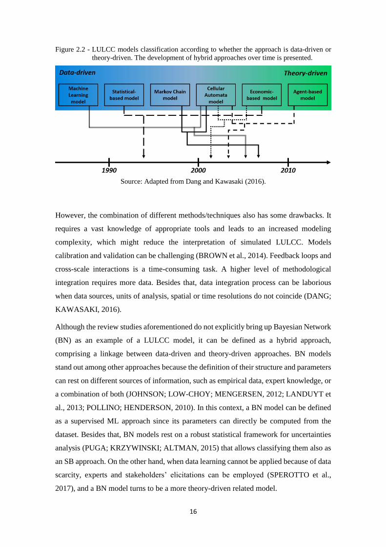
Figure 2.2 - LULCC models classification according to whether the approach is data-driven
or theory-driven. The development of hybrid approaches over time is presented. . 16
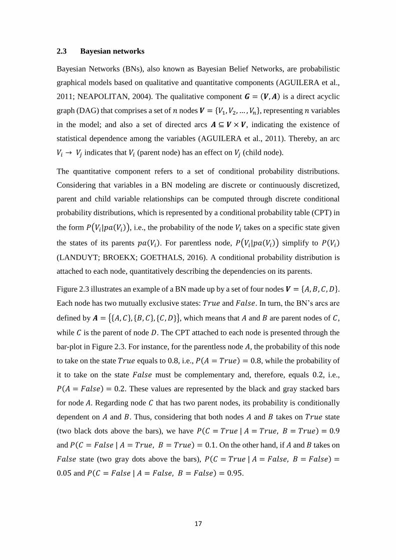
Figure 2.3 - Example of a BN model with four variables 𝐕 = {A, B, C, D} (on the left). Grey
colored node indicates an evidence presence by selecting a state C = true. Values
in other nodes are the posterior probabilities given such evidence. Bar plot (on the
right) illustrates the probability distributions attached to each variable.
Conditional probabilities for variables C and D describe dependencies on their
parents. .................................................................................................................... 18
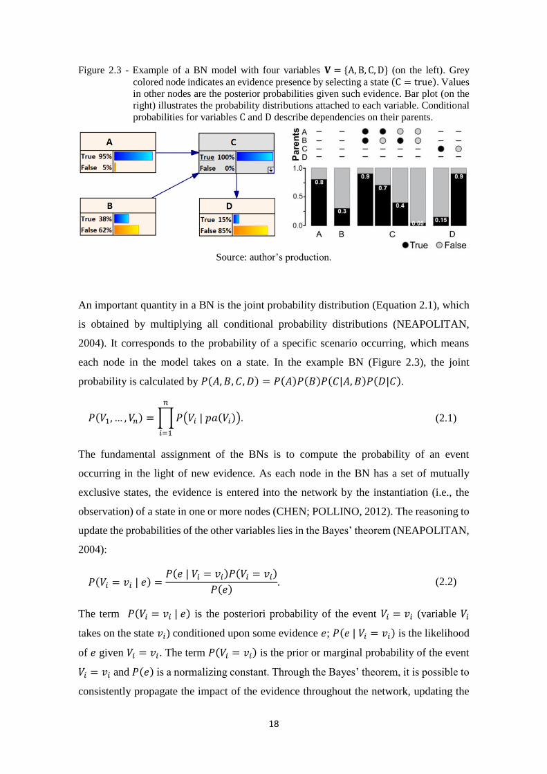
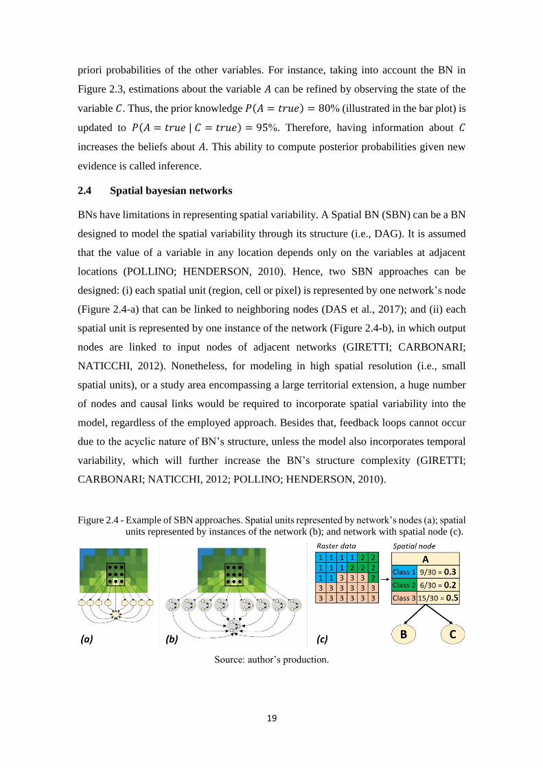
Figure 2.4 - Example of SBN approaches. Spatial units represented by network’s nodes (a);
spatial units represented by instances of the network (b); and network with spatial
node (c). .................................................................................................................. 19
Figure 2.5 - Example of a Dynamic Bayesian Network (DBN). A collapsed DBN (a); and an
unrolled DBN in three time-slices (b). Full-filled black arrows indicate non-
temporal arcs, while the red dashed arrows are temporal arcs. ............................... 22
Figure 2.6 - Example of STBN approaches. Spatial units represented by network’s node (a);
spatial units represented by instances of networks (b); and spatio-temporal node
(c). ........................................................................................................................... 27
Figure 3.1 - General workflow of the stbnR package. Blue boxes represent procedures, while
yellow boxes represent input/outputs. ..................................................................... 30
Figure 3.2 - The example STBN model. It is composed of A, B, C, and D nodes in two different
time-slices. Full-filled black arrows indicate non-temporal arcs, while the red
dashed arrows are temporal arcs. ............................................................................ 31
Figure 3.3 - Raster data of the variables included in the example STBN model. On the left –
A, C, and D are discrete spatio-temporal variables. The first column shows how
these variables were spatially distributed at time-slice t − 1. The second column
shows how these variables were spatially distributed in the next time-slice t. On
the right – B is a continuous static spatial variable. The mask defines the region
of interest (ROI). ..................................................................................................... 32
Figure 3.4 - Settings file. Specifications for each node in the example STBN model are
presented. ................................................................................................................ 34
Figure 3.5 - Graphical point-and-click interfaces for the user interact with to define nodes’
relationships. The example STBN model as illustrated in Figure 3.2 is designed.
The graphical interface to define non-temporal arcs (a), and the graphical
interface to define temporal arcs (b). In (b) time-slices are differentiated by colors.
................................................................................................................................. 38
Figure 3.6 - Prior probability distribution of node Dt − 1 (a), and the conditional probability
of node. Dt − 1 given the node Ct − 1(b). .............................................................. 40
Figure 3.7 - Conditional probability tables attached to nodes of the example STBN model. ..... 41
Figure 3.8 - The rolling up process for an STBN. For each iteration, a new time-slice is added
in front of the STBN, while the last one is removed (gray time-slices). ................. 43
Figure 4.1 - Regions of interest located in the Brazilian Legal Amazon. Amazonas state (a);
Mato Grosso state (b); and Pará state (c). Red-colored regions correspond to
xiv
deforested areas until 2018. Green-colored regions are forest areas. Yellow-
colored regions represent non-forest areas. ........................................................ 47
Figure 4.2 - Masks used to define case study regions. Amazon case study mask (a); Mato
Grosso case study mask (b); and Pará case study mask (c). Black-colored areas
correspond to regions of no interest. ....................................................................... 50
Figure 4.3 - Settings file employed in all case studies. ............................................................... 54
Figure 4.4 - First-order Markov STBN. Blue-colored nodes represent temporal nodes, while
yellow-colored nodes represent static nodes. Black fulfilled lines represent non-
temporal arcs, while red dotted lines represent temporal arcs. ............................... 56
Figure 4.5 - First-order Markov STBN. Blue-colored nodes represent temporal nodes, while
yellow-colored nodes represent static nodes. Black fulfilled lines represent non-
temporal arcs. In turn, red dotted lines represent temporal arcs between a one-
time interval, while blue dashed lines represent temporal arcs between a two-time
interval. ................................................................................................................... 57
Figure 5.1 - Probability images time series resulting from the first-order Markov STBN in the
Amazon case study. ............................................................................................ 62
Figure 5.2 - Probability images time series resulting from the second-order Markov STBN in
the Amazon case study. ........................................................................................... 63
Figure 5.3 - Variables importance according to the MI for the first-order Markov STBN in the
Amazonas case study. ............................................................................................. 64
Figure 5.4 - Distribution of the predicted probability values for deforestation and forest pixels
selected for accuracy assessment in the Amazonas case study. On the left, for the
first-order Markov STBN, and second-order Markov STBN on the right. ............. 65
Figure 5.5 - Assessment metrics of the STBNs predictions in the Amazon case study. Fulfilled
lines represent assessment metrics of the First-order Markov STBN model
predictions, while dashed lines represent assessment metrics of the Second-order
Markov STBN model predictions. Red lines refer to AUC-ROC values, while
green and blue lines refer to Kappa and Precision values, respectively. ................. 66
Figure 5.6 - Probability images time series resulting from the first-order Markov STBN in the
Mato Grosso case study. ......................................................................................... 67
Figure 5.7 - Probability images time series resulting from the second-order Markov STBN in
the Mato Grosso case study. .................................................................................... 68
Figure 5.8 - Variables importance according to the MI for the first-order Markov STBN in the
Mato Grosso case study. ......................................................................................... 69
Figure 5.9 - Distribution of the predicted probability values for deforestation and forest pixels
selected for accuracy assessment in the Mato Grosso case study. On the left, for
the first-order Markov STBN, and second-order Markov STBN on the right. ....... 70
Figure 5.10 - Assessment metrics of the STBNs predictions in the Mato Grosso case study.
Fulfilled lines represent assessment metrics of the First-order Markov STBN
model predictions, while dashed lines represent assessment metrics of the
Second-order Markov STBN model predictions. Red lines refer to AUC-ROC
values, while green and blue lines refer to Kappa and Precision values,
respectively. ............................................................................................................ 71
Figure 5.11 - Probability images time series resulting from the first-order Markov STBN in
the Pará case study. ................................................................................................. 72
Figure 5.12 - Probability images time series resulting from the second-order Markov STBN in
the Pará case study. ................................................................................................. 73
xv
Figure 5.13 - Variables importance according to the MI for the first-order Markov STBN in
the Pará case study. ................................................................................................. 74
Figure 5.14 - Distribution of the predicted probability values for deforestation and forest pixels
selected for accuracy assessment in the Pará case study. On the left, for the first-
order Markov STBN, and second-order Markov STBN on the right. ..................... 75
Figure 5.15 - Assessment metrics of the STBNs predictions in the Pará case study. Fulfilled
lines represent assessment metrics of the First-order Markov STBN model
predictions, while dashed lines represent assessment metrics of the Second-order
Markov STBN model predictions. Red lines refer to AUC-ROC values, while
green and blue lines refer to Kappa and Precision values, respectively. ................. 75
Figure 5.16 - Processing time of the STBN approaches in each case study. Orange bars refer
to the bottleneck step processing time, while the green bars refer to the remaining
steps of the entire modeling. ................................................................................... 77
Figure B.1 - Mean of the AUCROC, Precision, and Kappa metrics by STBN models and by
case studies with standard deviation error bars. .................................................... 100

xvi
xvii
LIST OF TABLES
Table 3.1 - BuildDataFrame function. ........................................................................................ 35
Table 3.2 - BuildDataFrame function result for the example data. ............................................. 36
Table 3.3 - BuildSTBN function. ................................................................................................ 37
Table 3.4 - QuerySTBN function. ............................................................................................... 42
Table 3.5 - TargetMapping function. .......................................................................................... 45
Table 4.1 - Target and context variables with their original format and source.......................... 51
Table 4.2 - Settings file specifications. (to be continued) .......................................................... 55
Table 4.3 - A confusion matrix used to evaluate presence-absence models. .............................. 58
Table 4.4 - Assessment metrics calculated from the confusion matrix. ...................................... 58
Table 5.1 - Processing time of the STBN approaches. ................................................................ 77
Table A.1 - Assessment metrics of the STBNs predictions in the Amazon case study. ............. 97
Table A.2 - Assessment metrics of the STBNs predictions in the Mato Grosso case study. ...... 97
Table A.3 - Assessment metrics of the STBNs predictions in the Pará case study. .................... 97
Table B.1 - AUC-ROC, Precision, and Kappa metrics mean and standard deviation for the STBN
models. The p-value obtained from the independent t-test is also shown. .............. 99

xviii

xix
LIST OF ABBREVIATIONS
AB – Agent-based
AI Artificial Intelligence
ANN – Artificial Neural Network
AUC-ROC – Area Under the Receiver Operating Characteristic curve
AWIFS – Advanced Wide Field Sensor
BLA – Brazilian Legal Amazon
BN – Bayesian Network
CA – Cellular Automata
CBERS – China-Brazil Earth-Resources Satellite
CPT – Conditional Probability Table
CRAN – Comprehensive R Archive Network
DBN – Dynamic Bayesian Network
DETER – Near Real-Time Deforestation Detection System
DT – Decision Tree
EB – Economic-base
EBF – Evidential Belief Function
FR – Frequency Ratio
GAM – Generalized Additive Model
GIS – Geographic Information System
INPE – National Institute for Space Research
LAI – Leaf Area Index
LR – Logistic Regression
LULCC – Land Use Land Cover Change
MC – Markov Chain
ML – Machine Learning
MODIS – Moderate-Resolution Imaging Spectroradiometer
PPCDAm – Action Plan to Prevent and Control Deforestation in Amazon
PRODES – Brazilian Amazon forest monitoring by satellite
RF – Random Forest
ROC – Receiver Operating Characteristic
ROI – Region of Interest
SB – Statistical-based
SBN – Spatial Bayesian Network
STBN – Spatio-Temporal Bayesian Network
SVM – Support Vector Machine
WFI – Wide Field Imager
WoE – Weights of Evidence

xx
xxi
CONTENTS
1. INTRODUCTION ............................................................................................................... 1
2. LITERATURE REVIEW ................................................................................................... 4
2.1 Amazon forest environmental governance .................................................................... 4
2.2 Land use and land cover change models ....................................................................... 8
2.2.1 Machine learning ................................................................................................. 10
2.2.2 Statistical-based ................................................................................................... 11
2.2.3 Markov chains ..................................................................................................... 11
2.2.4 Cellular automata ................................................................................................ 12
2.2.5 Economic-based .................................................................................................. 13
2.2.6 Agent-based ......................................................................................................... 14
2.2.7 Hybrid approaches ............................................................................................... 15
2.3 Bayesian networks....................................................................................................... 17
2.4 Spatial bayesian networks ........................................................................................... 19
2.5 Dynamic bayesian networks ........................................................................................ 21
2.6 Spatio-temporal bayesian networks............................................................................. 25
3. SPATIO-TEMPORAL BAYESIAN NETWORK FOR R (stbnR) ............................... 29
3.1 Input raster data ........................................................................................................... 31
3.2 Settings file .................................................................................................................. 33
3.3 Formatted data ............................................................................................................. 34
3.4 STBN model training .................................................................................................. 36
3.4.1 STBN graphical model definition ....................................................................... 37
3.4.2 Conditional probability tables computation ........................................................ 39
3.5 STBN query ................................................................................................................ 41
3.6 STBN model outputs ................................................................................................... 44
4 STBN MODELS FOR DEFORESTATION RISK PREDICTION .............................. 46
4.1 Case study regions ....................................................................................................... 46
4.1.1 Amazonas case study .......................................................................................... 47
4.1.2 Mato Grosso case study ....................................................................................... 47
4.1.3 Pará case study .................................................................................................... 48
4.2 Dataset and pre-processings ........................................................................................ 48
4.3 Building the STBN models ......................................................................................... 54
4.4 STBN models assessment ........................................................................................... 58
5 RESULTS AND DISCUSSION ........................................................................................ 61
5.1 Amazonas case study .................................................................................................. 62
5.2 Mato Grosso case study ............................................................................................... 66
5.3 Pará case study ............................................................................................................ 71
5.4 Processing time analysis .............................................................................................. 76
6 CONCLUSION .................................................................................................................. 78
REFERENCES .......................................................................................................................... 80
APPENDIX A: ASSESSMENT METRICS OF THE STBN MODELS PREDICTIONS. . 97
APPENDIX B: HYPOTHESIS TESTING FOR THE ASSESSMENT METRICS. ........... 98
1
1. INTRODUCTION
Artificial Intelligence (AI) systems should be able to reason probabilistically to cope with
uncertainties that may affect the results of any modeling. The probability theory is a
suitable foundation for representing the strengths of beliefs and summarize uncertainties
that may come from various sources. The key tool for dealing with probabilities in AI is
the Bayesian Network (BN), which is a type of probabilistic graphical model capable of
representing the dependency relationship among variables with an explicit treatment of
uncertainty by means of probabilities. This makes the BNs a suitable approach for
probabilistic reasoning of multiple areas.
BNs are acknowledged for their unique probabilistic modeling approach and their high
model transparency (LANDUYT et al., 2013). They provide an intuitive graphical
representation of the variables conditional dependencies via a directed acyclic graph.
Since variables’ relationships are graphically represented, the BN’s semantic facilitates
the understanding and the decision-making process for the users (DE SANTANA et al.,
2007). A BN also provides an inference mechanism, which is possible thanks to
conditional probability distributions that quantify the causal relationships between the
network variables. The usefulness of BNs lies in the fact that by using Bayes’ theorem,
one can proceed not only from causes to consequences but also deduce the probabilities
of different causes given the consequences (UUSITALO, 2007).
Additionally, BNs can model complex systems with a large number of variables, besides
to handle small and incomplete data sets and perform proper predictions. In case of a lack
of sufficient empirical data, expert and stakeholder knowledge can be incorporated via a
participatory modeling procedure (AGUILERA et al., 2011; LANDUYT et al., 2013).
Notwithstanding such advantages, BNs present some limitations. BNs do not explicitly
model the spatial domain. However, the states of a phenomenon in the field of Earth
observation, for example, may have some spatial variability. To represent changes in
space statically, the solution is straightforward so that BN and Geographic Information
System (GIS) are integrated to overcome BN’s weakness in representing spatially
distributed variables. This approach, known as Spatial BN (SBN), confers to the BN a
spatially explicit strategy, but it only permits to reproduce static changes through space
(SPEROTTO et al., 2017).
2
A BN also does not explicitly model temporal relationships between variables. The
probabilistic reasoning is carried out at a particular point in time and, therefore, a BN is
actually a static model. The only way to relate a variable with its past or future is by
replicating it for each time-step and assigning a time index to it. Consequently, we have
to work with a given discrete time scale to adapt the BN as a Markovian process. A
Markov process is any stochastic process that satisfies the Markov property that the
current state depends on only a finite fixed number of previous states. The simplest one
is a first-order Markov process, in which the current state depends only on the previous
state and not on any earlier state (RUSSELL; NORVING, 2010). One way of extending
Markov models is to allow higher-order interactions between variables.
Even with the Markov property, there is a classical problem when working with BNs in
the temporal domain: do we need to specify a different conditional probability distribution
for each time-step? To avoid this problem, we assume that changes in the world state are
caused by a stationary process, i.e., a process of change that is driven by laws that do not
themselves change over time (DE SANTANA et al., 2007; RUSSELL; NORVING,
2010). A BN replicated over time that satisfies the Markov property and is stationary is
know as a Dynamic Bayesian Network (DBN). Hence, DBNs extend the concept of BNs
by relating variables across time.
Therefore, the SBN and DBN overcome BN’s weaknesses of not explicitly model spatial
and temporal relationships between variables, respectively. However, space and time play
a crucial role in monitoring and managing environmental systems and, thus, should not
be considered separately. To that end, a Spatio-Temporal Bayesian Network (STBN)
seems to be an appropriate approach to combine the spatial and temporal variability of a
spatio-temporal process, such as deforestation, into the BN modeling.
SBNs have been employed in the land-use and land-cover changes (LULCC) modeling
(CELIO; KOELLNER; GRÊT-REGAMEY, 2014), as well as to predict deforestation risk
(DLAMINI, 2016; KRÜGER; LAKES, 2015; MAYFIELD et al., 2017). However, in
these studies, deforestation has been considered as a static process, in which the temporal
domain is not taken into account. An attempt to fill this gap was made by Silva et al.
(2020), in which the authors presented a stepwise application of an SBN approach over
time, which can be seen as a snapshot model for each moment. In this way, the temporal
dynamics of deforestation processes was not directly incorporated into the modeling. In
fact, static SBN modeling was carried out in each step.
3
In this context, the main goal of this work is to build STBN models to predict
deforestation risk areas. To accomplish that, we assume the hypothesis that STBN-based
LULCC models are able to represent and capture the variables’ spatio-temporal
relationships to appropriately predict deforestation risk. The STBN models developed in
this work ware tested to predict deforestation risk in three deforestation frontiers in the
Amazon forest: (i) in the southwestern of Amazon state, (ii) in the northwestern of Mato
Grosso state, and (iii) in the southwestern of Pará state. Within the context of this study,
we define Amazon deforestation as the total removal of primary forests (clear cut).
In order to develop the STBN-based LULCC models, we implemented in the context of
this thesis the package named stbnR (Spatio-Temporal Bayesian Network for R), which
enables the development of STBN-based LULCC models within the R environment. The
stbnR package was developed in R because it is a constantly evolving open-source
programming language. This allows anyone to test and contribute to improvements to the
stbnR package. Furthermore, R is a powerful language for statistical computing and
analysis and has available a massive collection of packages to support the development
of new ones.
Therefore, this thesis presents mainly three contributions. First, we encompass the
temporal domain into the LULCC modeling, specifically in the prediction of deforestation
risk. Second, we implemented the stbnR package, which enables the development of
STBN-based LULCC models within the R environment for other earth observation
applications besides the deforestation process. And third, we proposed a new approach
for predicting deforestation risk areas based on the Spatio-Temporal Bayesian Network
(STBN).
This thesis is organized as follows. This first chapter provides the context, contribution,
hypothesis, and objective of the work. Chapter 2 presents an overview of the Brazilian
Amazon environmental governance as well as a taxonomy of LULCC models and BN
approaches. Chapter 3 provides a detailed description of the stbnR package functions,
while Chapter 4 describes the case studies in addition to the dataset used and pre-
processings carried out. Chapter 5 presents the results of each case study. Finally, Chapter
6 concludes this thesis with an overview of the work.
4
2. LITERATURE REVIEW
2.1 Amazon forest environmental governance
Amazon Biome encompasses an area of about 6.7 million km2 shared by nine countries:
Brazil, Bolivia, Peru, Ecuador, Colombia, Venezuela, Guyana, Suriname, and French
Guiana, with the majority area inside Brazilian boundaries. The Amazon rainforest covers
most of the Amazon Biome, being the most extensive continuous remaining tropical
forest in the globe. Much attention has been given to this region since it provides unique
environmental services, houses at least one in ten of the world’s known biodiversity, and
plays a critical role in maintaining climate functions regionally and globally (ALVES et
al., 2017; NOBRE; BORMA, 2009; WWF, 2019).
In Brazil, an anthropization process started in the 1960s in response to the government
policies to integrate the Amazon region with the rest of the country (SHIMABUKURO
et al., 2012). In 1966, the government instituted the Brazilian Legal Amazon1 (BLA),
which corresponds to more than 60% of the Brazilian territory, encompassing the states
of Acre, Amapá, Amazonas, Mato Grosso, Pará, Rondônia, Tocantins, and the western
part of Maranhão state (BRASIL, 2007), hence, including the Brazilian Amazon biome
and part of the Cerrado and Pantanal Biomes. BLA’s territorial boundaries have a
sociopolitical rather than geographical bias as it was established as a way to plan and
promote the social and economic development of the region (IBGE, 2014).
Such integration process was carried out mainly through the construction of a massive
highway network, and migration incentive policies such as the National Development
Plans (SIMMONS, 2002). Consequently, this shifted the agricultural frontier towards the
Amazon region, creating the so-called arc of deforestation (SHIMABUKURO et al.,
2012). At the time, cattle ranching became a great investment choice, given the plentiful
and inexpensive lands, besides high world beef prices (SIMMONS, 2002). Afterward,
development policies in the Amazon region shifted toward mineral extraction, and during
the Brazilian government transition from a military regime to democracy in the 1980s,
1 The term "Legal Amazon" was only incorporated in recent legislations and is not explicitly stated in the laws that defined the Brazilian Amazon area for public policy purposes in previous decades. The use of the adjective "legal" is due to the need to differentiate the Amazon basin, Amazon Biome, as well as the International Amazon (IBGE, 2014).
5
concerns about forest loss increased as the incentive to economic development also
presented several environmental damages (ARIMA et al., 2014; SIMMONS, 2002).
In the late 1980s, indigenous rights got much attention, which resulted in a significant
number of indigenous reserves along with some conservation units (SIMMONS, 2002).
Additionally, the National Institute for Space Research (INPE) started to monitor the
BLA with satellite images, reporting yearly deforestation rates, which the Brazilian
government has been using as an indicator for proposing environmental public policies
and for evaluating their effectiveness (INPE, 2019c). The Brazilian Forest Code was a
significant restriction on deforestation on private lands that established a minimum
portion of each property (20 to 50%) that should be kept as a forest reserve (NEPSTAD
et al., 2014). Nevertheless, in 1995, INPE announced the largest deforestation rate in
history (INPE, 2019a). The president at the time increased forest reserves portion in the
properties to 80%, making compliance practically unattainable and reducing the law’s
credibility (NEPSTAD et al., 2014). Although rates declined in the following years,
Amazon deforestation became far more sensitive to commodity market conditions, and
technological advances favored the large-scale expansion of mechanizes crops, mainly
soybean, whose prices spiked in the early 2000s, so did deforestation rates, which
returned to the high levels in 2004 (ARIMA et al., 2014; NEPSTAD et al., 2014).
After deforestation rates in the BLA sharply increased in 2004, the Brazilian government
implemented the Action Plan to Prevent and Control Deforestation in Amazon
(PPCDAm-I) (BRASIL, 2004). Deforestation rates declined in the following years, but
this trend reversed in 2008 (INPE, 2019a), and the government instituted the PPCDAm-
II (BRASIL, 2009). Deforestation reduction became the central issue in the government
climate change agenda, and the implemented environmental public policies produced
significant externalities such as the restructuring of Brazil’s environmental enforcement
agency (IBAMA) and the expansion of the protected areas network and indigenous lands
(ARIMA et al., 2014; MELLO; ARTAXO, 2017).
Along with these government actions, other factors also influenced deforestation
reduction. In 2004, law enforcement capacity increased with the release of a real-time
deforestation detection system (DETER) by INPE (SHIMABUKURO et al., 2012). In
2005, the profitability of soybean production plummeted (NEPSTAD et al., 2014), as well
as the cattle ranching (ARIMA et al., 2014). In the next year, the Soy Moratorium was
established (GIBBS et al., 2015), and the Term of Adjustment of Conduct for
6
meatpacking companies was signed in 2009 (CARVALHO et al., 2019). Both were
agreements to block the commercialization of soybean and cattle, respectively, from
deforested areas. As a result of all those factors, deforestation in BLA reached the lowest
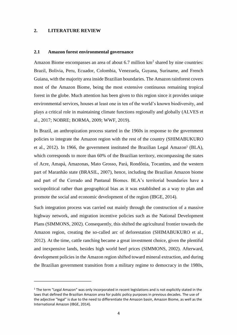
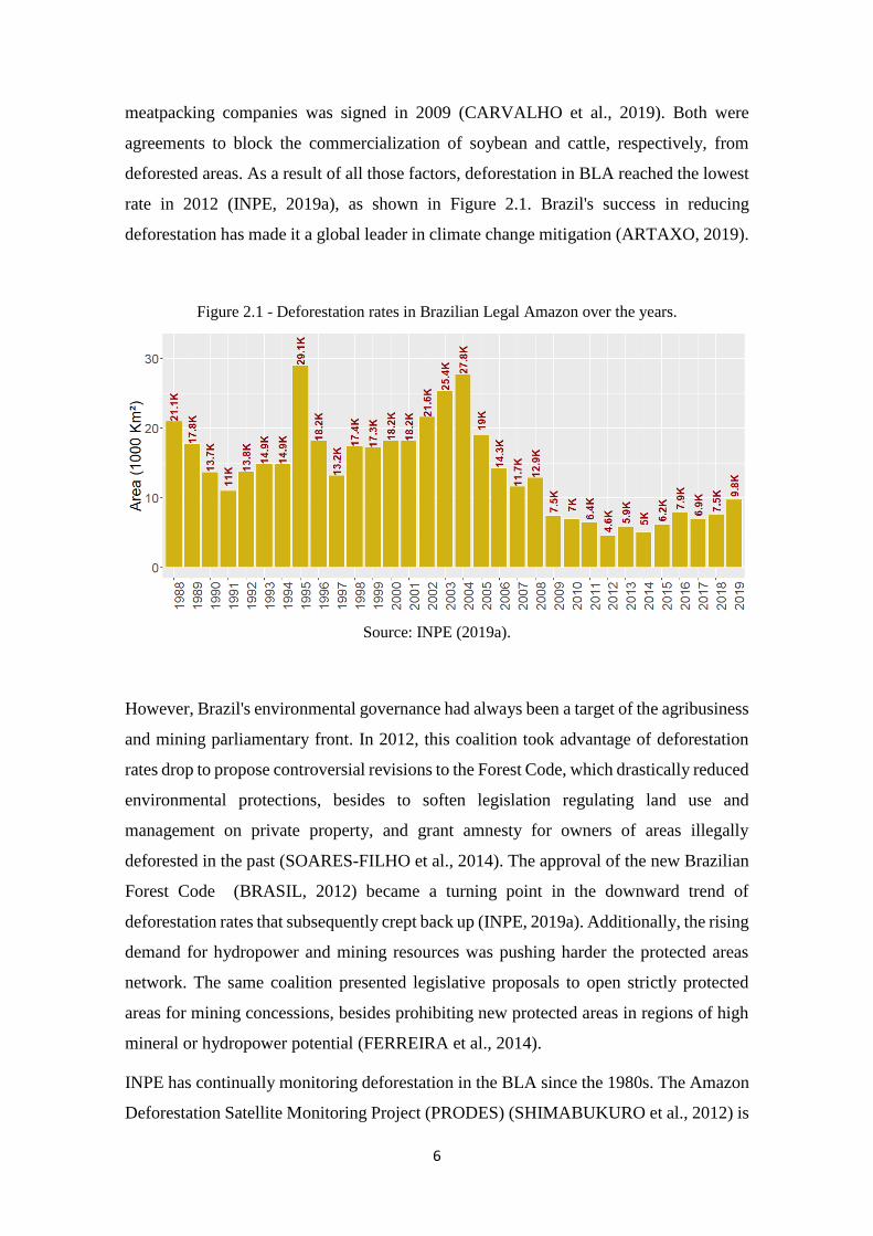
rate in 2012 (INPE, 2019a), as shown in Figure 2.1. Brazil's success in reducing
deforestation has made it a global leader in climate change mitigation (ARTAXO, 2019).
Figure 2.1 - Deforestation rates in Brazilian Legal Amazon over the years.
Source: INPE (2019a).
However, Brazil's environmental governance had always been a target of the agribusiness
and mining parliamentary front. In 2012, this coalition took advantage of deforestation
rates drop to propose controversial revisions to the Forest Code, which drastically reduced
environmental protections, besides to soften legislation regulating land use and
management on private property, and grant amnesty for owners of areas illegally
deforested in the past (SOARES-FILHO et al., 2014). The approval of the new Brazilian
Forest Code (BRASIL, 2012) became a turning point in the downward trend of
deforestation rates that subsequently crept back up (INPE, 2019a). Additionally, the rising
demand for hydropower and mining resources was pushing harder the protected areas
network. The same coalition presented legislative proposals to open strictly protected
areas for mining concessions, besides prohibiting new protected areas in regions of high
mineral or hydropower potential (FERREIRA et al., 2014).
INPE has continually monitoring deforestation in the BLA since the 1980s. The Amazon
Deforestation Satellite Monitoring Project (PRODES) (SHIMABUKURO et al., 2012) is
7
an internationally recognized INPE’s monitoring systems that map the clear-cutting
deforestation (when there is the complete removal of the forest cover) to compute the
official yearly deforestation rates. Despite that, PRODES methodology (CÂMARA et al.,
2013) requires time to produce such data, which rule out the rapid intervention from
government and environmental control agencies to stop illegal deforestation activities.
To get around this, INPE created the Near Real-Time Deforestation Detection System
(DETER) to exploit the high temporal resolution of nearly daily coverage of the MODIS
sensor at 250 𝑚 spatial resolution (SHIMABUKURO et al., 2012). The DETER system
was designed to be an early warning system to support surveillance and control of
deforestation, mapping the occurrence of forest degradation and clear-cutting areas
greater than 25 ha (DINIZ et al., 2015). However, the reduction in the average size of
deforested areas over the years became a major limitation for MODIS-based
methodology. Because of that, DETER system started using AWIFIS and WFI sensors
imageries at 56 𝑚 and 64 𝑚 spatial resolutaion, respectively, both with 5 days temporal
resolution, to adapt to the changes in deforestation process (DINIZ et al., 2015).
Additionally, INPE maintains the TerraClass Project, which represents a concerted effort
to monitor LULCC in the BLA. The database used in this project comprises deforested
areas mapped under the PRODES Project, as well as LANDSAT5/TM images and
MODIS time-series. Based on information about deforestation dynamics, remote sensing,
and geoprocessing techniques, systemic maps of the use and coverage of deforested lands
in the BLA have been produced (ALMEIDA et al., 2016). INPE also supports the Wildfire
System that detects vegetation fires from different polar-orbiting and geostationary
satellites operationally processed in near-real-time (INPE, 2008, 2019b; SETZER et al.,
2012).
Given the overview in this chapter, one can be seen that the Amazon rainforest has been
under constant pressure despite numerous efforts to monitor it and mitigate deforestation.
As stated by Rochedo et al. (2018), “deforestation control is a result of forces arising from
institutional arrangements such as enforcing the rule of law and sending signals that may
[…] incentivize economic agents to decide whether or not to deforest illegally.” In
summary, environmental governance in Brazil can be separated into three majors periods:
before 2004, a period with weak governance and high deforestation rates; between 2005–
2012, when there were improvements in environmental governance with effective results
8
in reducing deforestation; and the period after 2013 when governance has been gradually
deteriorating (ROCHEDO et al., 2018).
2.2 Land use and land cover change models
Understanding LULCC is essential for effective natural resource management. Usually,
involved parties employ models to explore LULCC dynamics and driving factors, and to
support causes and consequences analysis of these changes in order to formulate proper
environmental policies. In addition to that, analyses of past LULCC provide necessary
information that may assist in comprehend current changes and can be used as parameters
to draft alternative scenarios of future LULCC.
LULCC modeling is a complex domain. As stated by Noszczyk (2018), it requires
interdisciplinary knowledge, familiarity with statistical and spatial data, and skill in
analyses and statistical methods. The selection of the appropriate approach depends on
various factors, such as research aims and problems, spatial and temporal scale, and data
availability (DANG; KAWASAKI, 2016; NOSZCZYK, 2018). Given the various
modeling approaches, choosing the appropriate one can be complicated. Hence, the
arrangement of models into similar conceptual approaches allows for a better
understanding of their advantages and limitations (CHANG-MARTÍNEZ et al., 2015).
Indeed, LULCC models can be classified in different ways. For instance, as spatial or
non-spatial models, which attempt to, respectively, explore the spatial distribution and
patterns of change (land allocation), or estimate the rates or quantity of change (land
demand) (DALLA-NORA et al., 2014; MAS et al., 2014). LULCC models can also be
arranged as static or dynamic. A static model is time-invariant, meaning that it considers
the modeled system in equilibrium (steady-state). In turn, a dynamic model is time-
dependent, accounting for changes in the system’s state over time (WAGNER et al.,
2019).
LULCC models can yet be classified as deterministic or stochastic. In deterministic
models, there is no randomness associated with it. The output is fully determined by
model parameters values and a given set of initial conditions. Therefore, the same model
run several times will always produce the same result (possibly repeated over time and
spatial units). Conversely, stochastic models, also known as probabilistic models, have
inherent randomness. Inputs are described by probability distributions as a way to
incorporate uncertainty into the model calculations, and the same parameter values and
9
initial conditions may lead to different outputs (ABIDEN et al., 2013; ROSA; AHMED;
EWERS, 2014; UUSITALO et al., 2015).
Several review studies have previously been produced to create LULCC model
taxonomies (VERBURG et al., 2004; HEISTERMANN; MÜLLER; RONNEBERGER,
2006; KOOMEN; RIETVELD; DE NIJS, 2008). More recently, Brown et al. (2012) and
Chang-Martínez et al. (2015) described LULCC models into two categories: according to
whether the approach is data-driven or theory-driven. The first category includes
inductive models, which are consistent in reproducing LULCC patterns, but weak in
explaining correlations (KOOMEN; BEURDEN, 2011). These models are empirically
fitted (training) from LULCC pattern data over space and time. The variable to be
predicted represents the LULCC, whereas predictor variables are factors or indicators that
may be related to the changes, such as accessibility (e.g., distance to roads), terrain
suitability (e.g., slope), public policies (e.g., protected areas), besides non-spatial data like
census data. The data-driven model’s output is a map of potential changes, and the
model’s evaluation is usually centered on the spatial comparison between observed and
simulation maps (BROWN et al., 2012; CHANG-MARTÍNEZ et al., 2015).
In turn, the theory-driven approach includes deductive models that are consistent in
explaining how and why LULCC will happen, but weak in the spatial allocation of the
change (KOOMEN; BEURDEN, 2011). Usually, theory-driven models rest on expert
knowledge and information about decision-making that leads to LULCC (process-based).
These models seek to represent the essential interactions between agents and their
environment, which means the model’s calibration consists of determining the agent’s
behavior rules. Simulation is fundamental to the theory-driven models. Having
prospective LULCC maps as output, theory-driven models can be evaluated by the same
methods as data-driven models do, but as the primary goal of these models is modeling
the change processes, their evaluation centers on agent’s rules for decision-making
(BROWN et al., 2012; CHANG-MARTÍNEZ et al., 2015).
In addition to those two categories, a hybrid modeling approach could also be defined,
representing a compromise between data-driven and theory-driven models. Indeed, there
are overlaps among modeling approaches, which complicates their exact classification
into one of those two categories. In this context and based on the reviews presented by
Brown et al. (2014), Dang and Kawasaki (2016), Michetti and Zampieri (2014), and
Noszczyk (2018), seven types of LULCC modeling approaches could be identified: (i)
10
machine learning; (ii) statistical-based; (iii) Markov chains; (iv) cellular automata; (v)
economic-based; (vi) agent-based; and (vii) hybrid approach. It is worthy of mentioning
that these approaches are not the only ones to cover the full range of LULCC modeling
approaches, but can be considered the key ones.
2.2.1 Machine learning
Machine learning (ML) models are powerful techniques for simulating and predicting
LULCC. They are computer algorithms developed to learn from data on how to carry out
a particular task automatically (ABURAS; AHAMAD; OMAR, 2019). Hence, ML
models are useful for situations where patterns data are available, and theory about
processes is scant (BROWN et al., 2014). In LULCC modeling, the learning is commonly
supervised and, consequently, both input (change-related variables) and output (change)
data must be provided to the ML model to build a functional relationship between these
data, capturing LULCC patterns. Unsupervised ML models are less common in LULCC
modeling (OMRANI et al., 2015).
As ML models are data-driven, there is a risk of overfitting. This happens when the model
fits too well to details of input data (training data) in a way that it fails in generalization
(BROWN et al., 2014). Even though, ML models are useful for extrapolations of the
functional relationship among variables under the strong assumption of a stationary
LULCC process, in which change patterns stay the same as in the precedent time (i.e.,
business-as-usual scenario). In this sense, the stationarity assumption turns to be a
limitation to ML models. New predictor variables might arise over time, and this cannot
be accounted for in the predictions. Moreover, calculated transitions rules cannot be
changed and be uninterpretable to the users as in an Artificial Neural Network (ANN),
which is known as a “black-box” model (DANG; KAWASAKI, 2016; NOSZCZYK,
2018).
ANNs plays a central role in the ML approaches (ABURAS; AHAMAD; OMAR, 2019),
but several ML techniques, such as Support Vector Machine (SVM), Decision Trees (DT)
(SAMARDŽIĆ-PETROVIĆ et al., 2017), Randon Forest (RF) (KAMUSOKO; GAMBA,
2015), ensemble approaches (BRADLEY et al., 2017), and even deep learning
approaches (CAO; DRAGIĆEVIĆ; LI, 2019; HELBER et al., 2018; ZHANG et al., 2019)
are also employed for LULCC modeling. ML models are commonly integrated with
process-based models, such as Cellular Automata (CA), to improve overall simulation
capabilities (BASSE et al., 2014; MUSTAFA et al., 2018).
11
2.2.2 Statistical-based
Statistical-based (SB) models are also dependent on data to delineate a relationship
between LULCC and predictor variables. Such a relationship is generally obtained
through linear or logistic regression, binomial or multinomial logit methods, among
others (DANG; KAWASAKI, 2016; NOSZCZYK, 2018). SB models assume a fixed
mathematical equation whose coefficients are estimated by a statistical process to produce
an optimal fit. That is, coefficients are estimated in order to a regression curve fits as
closely as possible to the data. Hence, coefficients indicate the influence of independent
variables regarding the dependent variable. SB models also provide a confidence degree
concerning the contribution of independent variables (BROWN et al., 2014; DANG;
KAWASAKI, 2016)
Some limitations might compromise the SB model's usefulness (BROWN et al., 2012).
Like ML models, SB models are built based on historical data, and they also assume a
stationary LULCC process to extrapolate the mathematical equation to the future.
However, SB models are limited in the ability to make out-of-sample predictions and are
not suitable for long-term and divergent scenarios. Also, spatial and temporal dependence
of data affects SB models (DANG; KAWASAKI, 2016; NOSZCZYK, 2018). SB models
are generally used to address linear problems (ABURAS; AHAMAD; OMAR, 2019), and
assumptions such as a log-linear relationship between independent and dependent
variables are required, which might be a limitation in modeling (BROWN et al., 2012).
Even though Logistic Regression (LR) is a widely used SB model in LULCC modeling
(ABURAS; AHAMAD; OMAR, 2019). Other SB models such as Frequency Ratio (FR),
Weights of Evidence (WoE), Evidential Belief Function (EBF) (AL-SHARIF;
PRADHAN, 2016; DING; CHEN; HONG, 2016; SOMA; KUBOTA; ADITIAN, 2019),
and non-linear methods, as Generalized Additive Model (GAM) (FENG; TONG, 2017;
SUN; ROBINSON, 2018) have also been employed to model LULCC.
2.2.3 Markov chains
Markov chain (MC) models provide a straightforward methodology by which a dynamic
system can be analyzed (KUMAR; RADHAKRISHNAN; MATHEW, 2014). MC
models are probably the most well-known approach for LULCC models rest on the
continuation of historical trends (BROWN et al., 2014), which means that these models
also work under the stationarity assumption. In a Markov process, the future system’s
state can be simulated purely based on the immediately preceding state. Hence, MC
12
models describe LULCC from one period to another and apply it to predict future changes
(KUMAR; RADHAKRISHNAN; MATHEW, 2014). To do so, these models employ a
stochastic transition matrix to represent all possible changes among LULCC classes. For
instance, three classes of LULCC result in a matrix 𝑀3𝑋3 with nine possible changes.
Transition matrix defines the probabilities of shifting from one LULCC category to
another. It can be obtained by comparing two maps of LULCC classes over time or by
expert knowledge (DANG; KAWASAKI, 2016; MAS et al., 2014).
Due to its simplicity, the MC model was a common approach in the early phase of
LULCC modeling (BROWN et al., 2014). However, a drawback of MC models is the
disregard of the LULCC spatial aspect, i.e., the assumption of spatial independence
(NOSZCZYK, 2018). Only cell states are considered, and the influence of neighboring
cells is not considered (DANG; KAWASAKI, 2016). To overcome this limitation, MC
models have been combined with GIS systems to spatialize the LULCC probabilities, and
several hybrid approaches have been proposed by merging MC models with other
approaches that simulate the spatial pattern of change, such as Cellular Automata
(KUMAR; RADHAKRISHNAN; MATHEW, 2014; LOSIRI et al., 2016; NASIRI et al.,
2018).
2.2.4 Cellular automata
Cellular automata (CA) models rest on a mathematical theory of self-reproduction in
automata and stochasticity within a two-dimension cellular-grid environment, which is
discrete in terms of time and space (DANG; KAWASAKI, 2016; NOSZCZYK, 2018). A
CA model consists of five elements: cell space, cell states, neighborhood, transition rules,
and time steps. The CA’s basic unit of simulation is the cell, and the set of cells make up
the cell space. In remote sensing and GIS fields, cells are usually concerned with pixels
or any other land unit. All the possible states that can be assigned to the cells correspond
to the cell states. Neighborhood defines which adjacent cells to a given cell will be
considered during the simulation. In turn, transition rules specify which new state will be
assigned to a given cell, taking into account neighboring cells states. Lastly, time step
concerns to a time interval between changes in the course of the simulation.
Underlying assumptions of CA models are the continuation of historical trends and
patterns, and allocation based on land suitability and neighborhood interaction (BROWN
et al., 2014). CA’s core principle is that the state of a given cell at time 𝑡 + 1 can be
13
determined by its state and neighboring cells states at time 𝑡 (NOSZCZYK, 2018).
Changes in each cell are simulated either rest on transition rules or some algorithm.
Transition rules can be derived from expert knowledge or statistical analysis. Unlike
ANNs, transition rules in CA models are clearly defined. In turn, an algorithm can be
employed to update cell states, representing decision-making. This algorithm is applied
synchronously to all cell space, and its output stems solely from the cell’s attributes
(BROWN et al., 2014; NOSZCZYK, 2018).
As CA are spatial models, they are compatible with most spatial data, easily integrated
with GIS, and allows to represent straightforward LULCC processes. On the other hand,
CA models are entirely reliant on the spatial unit, which means modeling results may
change with the variation of cell size and neighborhood configuration (NOSZCZYK,
2018). Nevertheless, CA models are widely used for LULCC modeling (ABURAS;
AHAMAD; OMAR, 2019). They are often combined with other modeling approaches
(MUSTAFA et al., 2017; RIMAL et al., 2018) besides being part of GIS software (MAS
et al., 2014; SOARES-FILHO; RODRIGUES; FOLLADOR, 2013).
2.2.5 Economic-based
Economic-based (EB) models stem from traditional economic theories and aim at
explaining changes in land-use patterns with economic-related variables, such as
production, consumption, prices, access to markets (MICHETTI; ZAMPIERI, 2014).
Hence, these models rest on the assumption that economics is the primary driver of
LULCC, and they do not usually take the climate and biophysical drivers into account.
Moreover, EB models consider that landowners will use the land to maximize the land’s
usefulness and expected profits (BROWN et al., 2014; NOSZCZYK, 2018). These
models also assume the equilibrium theory to estimate land changes considering the
demand-supply relationship (DANG; KAWASAKI, 2016; MICHETTI; ZAMPIERI,
2014). Some EB models can be distinguished by the scope of the economic system they
represent. A general equilibrium model represents the global economy, while partial
equilibrium models consider detailed descriptions of specific sectors, such as agriculture
or forestry production (BROWN et al., 2014; REN et al., 2019).
EB models can describe and quantify the influence of LULCC drivers on land demand.
Besides that, they provide the means for exploring the interactions within the human-
environment system, as well as for accessing the consequences of policies and decisions
14
made regarding land uses and their probable effects (CHANG-MARTÍNEZ et al., 2015;
MICHETTI; ZAMPIERI, 2014). EB models' parameters are often estimated using
econometric methods. In other cases, parameters may be guided by either theory taken
from previous studies or a range of values to explore the model’s sensitivity (BROWN et
al., 2014). A drawback of EB models is that they do not take into full account the
geographical location of change (NOSZCZYK, 2018), as these models assume economics
as the primary driver of LULCC.
2.2.6 Agent-based
Agent-based (AB) models, often called as multi-agent systems, describe intelligent
agents, their environment, and possible interactions. Agents are discrete entities
characterized by their attributes and their behaviors. They can interact with each other
and with the environment to collect information or carry out actions that modify their
context. Regarding the LULCC, agents could be landowners, households, farmers,
policy-making bodies, or any actors that make decisions or take actions that affect the
LULCC patterns (BROWN et al., 2014). AB models allow modelers to capture the
stakeholder's specialized knowledge and perform scenario analysis (DANG;
KAWASAKI, 2016). Hence, an AB model for LULCC consists of a map of the area of
interest and a model with agents representing human decision-making in a very flexible
and context-dependent way (GROENEVELD et al., 2017; NOSZCZYK, 2018).
As stated by Groeneveld et al. (2017), the majority of human decisions AB models for
LULCC are not explicitly based on theory, and the flexibility of these models comes along
with ad hoc assumptions of the decision process. AB models facilitate modeling of
feedback loops between human and environmental systems. Any interaction in AB
models is based on prescribed rules whose descriptions can be difficult and controversial.
For instance, agent preferences may be determined by expert judgment with questionnaire
surveys. Apart from expert knowledge, AB models facilitate the integration of other data
sources, such as current trends and existing models (NOSZCZYK, 2018). However, these
models tend to concentrate on the most readily apparent and quantifiable aspects of
LULCC and do not account for factors such as outmigration, changes in techniques and
input use, and the influence of regional and global economic variables (DANG;
KAWASAKI, 2016).
15
2.2.7 Hybrid approaches
No single model can take all LULCC characteristics into account owing to the complex
nature of it. In light of this, a hybrid approach, i.e., a merger of two or more individuals
models, is employed to represent the various aspect of LULCC patterns and processes
(BROWN et al., 2014; NOSZCZYK, 2018). Hybrid approaches take advantage of the
strengths of individual ones in order to reduce some of their inherent limitations, allowing
better representation of the LULCC (BROWN et al., 2014). As stated by Dang and
Kawasaki (2016), combining the best aspect of different approaches helps to cover several
disciplines, mutual relationships, and link social science with spatial data to represent the
LULCC process.
Broad diversity of hybrid approaches have evolved over the years. Figure 2.2 tries to
summarize the development of hybrid approaches for LULCC modeling with a relative
timing. The arrows indicate the approximate moment when two or more different
approaches were ensemble and employed in LULCC modeling, according to Dang and
Kawasaki (2016). Additionally, Figure 2.2 presents a rough arrangement of LULCC
models in terms of their emphasis on data-driven (blue zone) or theory-driven (green
zone).
Some hybrid approach achievements include solving problems of temporal and spatial
scale and covering multi-discipline and multi-scale approach (DANG; KAWASAKI,
2016). For example, an SB model like spatial regression can be used to solve spatial
mismatches between the imposition of regular boundaries on grid cells of a CA model.
On the other hand, an EB model is used to estimate land demand, while an ML model
like ANN is used to explain land allocation (DALLA-NORA et al., 2014; DANG;
KAWASAKI, 2016).
16
Figure 2.2 - LULCC models classification according to whether the approach is data-driven or
theory-driven. The development of hybrid approaches over time is presented.
Source: Adapted from Dang and Kawasaki (2016).
However, the combination of different methods/techniques also has some drawbacks. It
requires a vast knowledge of appropriate tools and leads to an increased modeling
complexity, which might reduce the interpretation of simulated LULCC. Models
calibration and validation can be challenging (BROWN et al., 2014). Feedback loops and
cross-scale interactions is a time-consuming task. A higher level of methodological
integration requires more data. Besides that, data integration process can be laborious
when data sources, units of analysis, spatial or time resolutions do not coincide (DANG;
KAWASAKI, 2016).
Although the review studies aforementioned do not explicitly bring up Bayesian Network
(BN) as an example of a LULCC model, it can be defined as a hybrid approach,
comprising a linkage between data-driven and theory-driven approaches. BN models
stand out among other approaches because the definition of their structure and parameters
can rest on different sources of information, such as empirical data, expert knowledge, or
a combination of both (JOHNSON; LOW-CHOY; MENGERSEN, 2012; LANDUYT et
al., 2013; POLLINO; HENDERSON, 2010). In this context, a BN model can be defined
as a supervised ML approach since its parameters can directly be computed from the
dataset. Besides that, BN models rest on a robust statistical framework for uncertainties
analysis (PUGA; KRZYWINSKI; ALTMAN, 2015) that allows classifying them also as
an SB approach. On the other hand, when data learning cannot be applied because of data
scarcity, experts and stakeholders’ elicitations can be employed (SPEROTTO et al.,
2017), and a BN model turns to be a more theory-driven related model.
17
2.3 Bayesian networks
Bayesian Networks (BNs), also known as Bayesian Belief Networks, are probabilistic
graphical models based on qualitative and quantitative components (AGUILERA et al.,
2011; NEAPOLITAN, 2004). The qualitative component 𝑮 = (𝑽, 𝑨) is a direct acyclic
graph (DAG) that comprises a set of 𝑛 nodes 𝑽 = {𝑉1, 𝑉2, … , 𝑉𝑛}, representing 𝑛 variables
in the model; and also a set of directed arcs 𝑨 ⊆ 𝑽 × 𝑽, indicating the existence of
statistical dependence among the variables (AGUILERA et al., 2011). Thereby, an arc
𝑉𝑖 → 𝑉𝑗 indicates that 𝑉𝑖 (parent node) has an effect on 𝑉𝑗 (child node).
The quantitative component refers to a set of conditional probability distributions.
Considering that variables in a BN modeling are discrete or continuously discretized,
parent and child variable relationships can be computed through discrete conditional
probability distributions, which is represented by a conditional probability table (CPT) in
the form 𝑃(𝑉𝑖|𝑝𝑎(𝑉𝑖)), i.e., the probability of the node 𝑉𝑖 takes on a specific state given
the states of its parents 𝑝𝑎(𝑉𝑖). For parentless node, 𝑃(𝑉𝑖|𝑝𝑎(𝑉𝑖)) simplify to 𝑃(𝑉𝑖)
(LANDUYT; BROEKX; GOETHALS, 2016). A conditional probability distribution is
attached to each node, quantitatively describing the dependencies on its parents.
Figure 2.3 illustrates an example of a BN made up by a set of four nodes 𝑽 = {𝐴, 𝐵, 𝐶, 𝐷}.
Each node has two mutually exclusive states: 𝑇𝑟𝑢𝑒 and 𝐹𝑎𝑙𝑠𝑒. In turn, the BN’s arcs are
defined by 𝑨 = {{𝐴, 𝐶}, {𝐵, 𝐶}, {𝐶, 𝐷}}, which means that 𝐴 and 𝐵 are parent nodes of 𝐶,
while 𝐶 is the parent of node 𝐷. The CPT attached to each node is presented through the
bar-plot in Figure 2.3. For instance, for the parentless node 𝐴, the probability of this node
to take on the state 𝑇𝑟𝑢𝑒 equals to 0.8, i.e., 𝑃(𝐴 = 𝑇𝑟𝑢𝑒) = 0.8, while the probability of
it to take on the state 𝐹𝑎𝑙𝑠𝑒 must be complementary and, therefore, equals 0.2, i.e.,
𝑃(𝐴 = 𝐹𝑎𝑙𝑠𝑒) = 0.2. These values are represented by the black and gray stacked bars
for node 𝐴. Regarding node 𝐶 that has two parent nodes, its probability is conditionally
dependent on 𝐴 and 𝐵. Thus, considering that both nodes 𝐴 and 𝐵 takes on 𝑇𝑟𝑢𝑒 state
(two black dots above the bars), we have 𝑃(𝐶 = 𝑇𝑟𝑢𝑒 | 𝐴 = 𝑇𝑟𝑢𝑒, 𝐵 = 𝑇𝑟𝑢𝑒) = 0.9
and 𝑃(𝐶 = 𝐹𝑎𝑙𝑠𝑒 | 𝐴 = 𝑇𝑟𝑢𝑒, 𝐵 = 𝑇𝑟𝑢𝑒) = 0.1. On the other hand, if 𝐴 and 𝐵 takes on
𝐹𝑎𝑙𝑠𝑒 state (two gray dots above the bars), 𝑃(𝐶 = 𝑇𝑟𝑢𝑒 | 𝐴 = 𝐹𝑎𝑙𝑠𝑒, 𝐵 = 𝐹𝑎𝑙𝑠𝑒) =
0.05 and 𝑃(𝐶 = 𝐹𝑎𝑙𝑠𝑒 | 𝐴 = 𝐹𝑎𝑙𝑠𝑒, 𝐵 = 𝐹𝑎𝑙𝑠𝑒) = 0.95.
18
Figure 2.3 - Example of a BN model with four variables 𝐕 = {A, B, C, D} (on the left). Grey
colored node indicates an evidence presence by selecting a state (C = true). Values
in other nodes are the posterior probabilities given such evidence. Bar plot (on the
right) illustrates the probability distributions attached to each variable. Conditional
probabilities for variables C and D describe dependencies on their parents.
Source: author’s production.
An important quantity in a BN is the joint probability distribution (Equation 2.1), which
is obtained by multiplying all conditional probability distributions (NEAPOLITAN,
2004). It corresponds to the probability of a specific scenario occurring, which means
each node in the model takes on a state. In the example BN (Figure 2.3), the joint
probability is calculated by 𝑃(𝐴, 𝐵, 𝐶, 𝐷) = 𝑃(𝐴)𝑃(𝐵)𝑃(𝐶|𝐴, 𝐵)𝑃(𝐷|𝐶).
𝑃(𝑉1, … , 𝑉𝑛) = ∏ 𝑃(𝑉𝑖 | 𝑝𝑎(𝑉𝑖))
𝑛
𝑖=1
. (2.1)
The fundamental assignment of the BNs is to compute the probability of an event
occurring in the light of new evidence. As each node in the BN has a set of mutually
exclusive states, the evidence is entered into the network by the instantiation (i.e., the
observation) of a state in one or more nodes (CHEN; POLLINO, 2012). The reasoning to
update the probabilities of the other variables lies in the Bayes’ theorem (NEAPOLITAN,
2004):
𝑃(𝑉𝑖 = 𝑣𝑖 | 𝑒) =𝑃(𝑒 | 𝑉𝑖 = 𝑣𝑖)𝑃(𝑉𝑖 = 𝑣𝑖)
𝑃(𝑒). (2.2)
The term 𝑃(𝑉𝑖 = 𝑣𝑖 | 𝑒) is the posteriori probability of the event 𝑉𝑖 = 𝑣𝑖 (variable 𝑉𝑖
takes on the state 𝑣𝑖) conditioned upon some evidence 𝑒; 𝑃(𝑒 | 𝑉𝑖 = 𝑣𝑖) is the likelihood
of 𝑒 given 𝑉𝑖 = 𝑣𝑖. The term 𝑃(𝑉𝑖 = 𝑣𝑖) is the prior or marginal probability of the event
𝑉𝑖 = 𝑣𝑖 and 𝑃(𝑒) is a normalizing constant. Through the Bayes’ theorem, it is possible to
consistently propagate the impact of the evidence throughout the network, updating the
19
priori probabilities of the other variables. For instance, taking into account the BN in
Figure 2.3, estimations about the variable 𝐴 can be refined by observing the state of the
variable 𝐶. Thus, the prior knowledge 𝑃(𝐴 = 𝑡𝑟𝑢𝑒) = 80% (illustrated in the bar plot) is
updated to 𝑃(𝐴 = 𝑡𝑟𝑢𝑒 | 𝐶 = 𝑡𝑟𝑢𝑒) = 95%. Therefore, having information about 𝐶
increases the beliefs about 𝐴. This ability to compute posterior probabilities given new
evidence is called inference.
2.4 Spatial bayesian networks
BNs have limitations in representing spatial variability. A Spatial BN (SBN) can be a BN
designed to model the spatial variability through its structure (i.e., DAG). It is assumed
that the value of a variable in any location depends only on the variables at adjacent
locations (POLLINO; HENDERSON, 2010). Hence, two SBN approaches can be
designed: (i) each spatial unit (region, cell or pixel) is represented by one network’s node
(Figure 2.4-a) that can be linked to neighboring nodes (DAS et al., 2017); and (ii) each
spatial unit is represented by one instance of the network (Figure 2.4-b), in which output
nodes are linked to input nodes of adjacent networks (GIRETTI; CARBONARI;
NATICCHI, 2012). Nonetheless, for modeling in high spatial resolution (i.e., small
spatial units), or a study area encompassing a large territorial extension, a huge number
of nodes and causal links would be required to incorporate spatial variability into the
model, regardless of the employed approach. Besides that, feedback loops cannot occur
due to the acyclic nature of BN’s structure, unless the model also incorporates temporal
variability, which will further increase the BN’s structure complexity (GIRETTI;
CARBONARI; NATICCHI, 2012; POLLINO; HENDERSON, 2010).
Figure 2.4 - Example of SBN approaches. Spatial units represented by network’s nodes (a); spatial
units represented by instances of the network (b); and network with spatial node (c).
Source: author’s production.
20
As any LULCC has a spatial dimension of interest, it should be considered in the
modeling. Thus, another approach to overcome BN’s weakness in representing
geographic information is by using spatial nodes (Figure 2.4-c). This type of node is
spatially described (JOHNSON; LOW-CHOY; MENGERSEN, 2012), and it summarizes
the spatial distribution of the variable through the probability distribution. This approach
confers to the BN a spatially explicit strategy, but it only permits to reproduce static
changes through space (SPEROTTO et al., 2017), representing the system and variables
relationships at a particular point in time (CHEN et al., 2019). In general, the LULCC
analysis relies on the use of static data from two points in time corresponding to the begin
and end of the time frame (WAGNER et al., 2019)
For each spatial node in the SBN, a raster layer from a GIS tool must be available. Hence,
it is useful to consider the integration of BNs with GIS. BN-GIS integration has gained
considerable interest over the years as the potential way to include spatial information
into the modeling (CHEN; POLLINO, 2012; LANDUYT et al., 2013). The connection between
BNs and GIS can be accomplished in different ways (JOHNSON; LOW-CHOY; MENGERSEN,
2012), but it is predominantly used to map BN’s outputs based on the georeferenced inputs
(LANDUYT et al., 2013). That means a GIS tool stores the raster data needed to parametrize
the BN, whose output is then computed for each location (region/cell/pixel as inputted
from GIS) to represent the outcomes in spatially explicit maps. Therefore, BN-GIS
integration allows for quantifying and visualizing the uncertainties associated with the
spatial system (LANDUYT et al., 2015).
Among the several BN software and packages available (KORB; NICHOLSON, 2010),
Netica and Hugin are commonly used in BN-GIS integration. The reviews presented by
Aguilera et al. (2011), Landuyt et al. (2013), and Pérez-Miñana (2016) demonstrate the
scientific community preference for the software Netica, followed by Hugin. For instance,
Grêt-Regamey and Straub (2006) embedded a BN from the Hugin software into the
ArcGIS to accesses the uncertainties involved in the avalanche run-out zones as well as
estimating the damage potential. Aitkenhead and Aalders (2009) applied an evolutionary
process to a BN developed from Netica with spatial input data extracted from ArcGIS to
predict LULCC. Stelzenmüller et al. (2010) used the Netica software to develop a BN-
GIS framework that supports marine spatial planning and evaluate the impact of human
activities on marine habitats.
21
To enhance the interaction between BN models and spatial data, Landuyt et al. (2015)
developed a plug-in that couples Netica and QGIS software to model spatial processes
and associated uncertainties. Balbi et al. (2016) proposed a BN-GIS framework
combining the software GeNIe and QGIS to assess the benefits of early warning for urban
flood risk to people. Likewise, Abebe, Kabir, and Tesfamariam (2018) embedded spatial
information from ArcGIS into the BN constructed from Netica to model the urban areas'
flood vulnerability. In turn, Sahin et al. (2019) presented an integrated approach
combining BNs developed on Netica, with input data extracted from ArcGIS spatial layers
to predict coastal erosion induced by sea-level rise.
Therefore, SBNs may integrate two tools: one to build the BN and another to deal with
spatial data. Those commonly used BNs software aforementioned (Netica and Hugin)
provide efficient Bayesian inference algorithms with a comprehensible user-friendly
interface. However, they are expensive when compared to open source software
(LANDUYT et al., 2015). Besides that, there are packages and libraries from specific
programming languages like R (R CORE TEAM, 2019) capable of dealing with both BNs
and spatial data in the same programming environment.
In this context, studies have employed R’s packages to create SBN methods for different
purposes. For instance, Mello et al. (2013) developed a method able to incorporate
expert’s knowledge and tested it on a case study for soybean crop mapping. This method
has been improved by Silva, Fonseca, and Körting, (2017) and applied it as a prediction
tool for identifying potential areas for sugarcane expansion. Gonzalez-Redin et al. (2016)
proposed a tool also developed with R’s packages to evaluate trade-offs between forest
production and conservation measures to preserve biodiversity in forested habitats. In
turn, Wijesiri et al. (2018) presented a spatial BN method to model urban water quality
and identify environmental and anthropogenic factors that pose risks to human health. All
these studies are pixel-based, which means the outputs of the proposed method are raster
layers, where pixels values correspond to occurrence probabilities of the studied
phenomenon.
2.5 Dynamic bayesian networks
In addition to spatial variability, it is also essential to model how the world changes over
time. However, BNs also have limitations in representing dynamic systems (POLLINO;
HENDERSON, 2010; UUSITALO, 2007). Due to the acyclic characteristics of its
structure (i.e., DAG), a BN is unable to represent feedback loops and systems that change
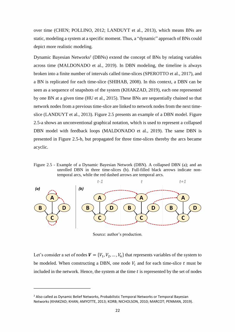
22
over time (CHEN; POLLINO, 2012; LANDUYT et al., 2013), which means BNs are
static, modeling a system at a specific moment. Thus, a “dynamic” approach of BNs could
depict more realistic modeling.
Dynamic Bayesian Networks2 (DBNs) extend the concept of BNs by relating variables
across time (MALDONADO et al., 2019). In DBN modeling, the timeline is always
broken into a finite number of intervals called time-slices (SPEROTTO et al., 2017), and
a BN is replicated for each time-slice (SHIHAB, 2008). In this context, a DBN can be
seen as a sequence of snapshots of the system (KHAKZAD, 2019), each one represented
by one BN at a given time (HU et al., 2015). These BNs are sequentially chained so that
network nodes from a previous time-slice are linked to network nodes from the next time-
slice (LANDUYT et al., 2013). Figure 2.5 presents an example of a DBN model. Figure
2.5-a shows an unconventional graphical notation, which is used to represent a collapsed
DBN model with feedback loops (MALDONADO et al., 2019). The same DBN is
presented in Figure 2.5-b, but propagated for three time-slices thereby the arcs became
acyclic.
Figure 2.5 - Example of a Dynamic Bayesian Network (DBN). A collapsed DBN (a); and an
unrolled DBN in three time-slices (b). Full-filled black arrows indicate non-
temporal arcs, while the red dashed arrows are temporal arcs.
Source: author’s production.
Let’s consider a set of nodes 𝑽 = {𝑉1, 𝑉2, … , 𝑉𝑛} that represents variables of the system to
be modeled. When constructing a DBN, one node 𝑉𝑖 and for each time-slice 𝑡 must be
included in the network. Hence, the system at the time 𝑡 is represented by the set of nodes
2 Also called as Dynamic Belief Networks, Probabilistic Temporal Networks or Temporal Bayesian Networks (KHAKZAD; KHAN; AMYOTTE, 2013; KORB; NICHOLSON, 2010; MARCOT; PENMAN, 2019).
23
𝑽𝒕 = {𝑉1𝑡, 𝑉2
𝑡 , … , 𝑉𝑛𝑡}. As variables can be related to each other at the same time-slice as
well as at successive time-slice, a DBN can present arcs connecting (i) different nodes at
the same time-slice, 𝑉𝑖𝑡 → 𝑉𝑗
𝑡; (ii) the same node over time, 𝑉𝑖𝑡 → 𝑉𝑖
𝑡+1; and (ii) different
nodes over time, 𝑉𝑖𝑡 → 𝑉𝑗
𝑡+1 (KORB; NICHOLSON, 2010).
Temporal variables that change over time and have effects on other variables in the future
are represented by temporal nodes in the DBN. These nodes are linked by temporal arcs
(i.e., arcs linking nodes from different time-slices). In turn, those static variables that do
not change over time and are related to others only in the current time-slice, are
represented by static nodes. In Figure 2.5, just 𝐵 is a static node, while 𝐴, 𝐶, and 𝐷 are
temporal nodes. One can observe that a DBN does not have backward links between
successive time-slices. Only forward temporal arcs are allowed, reflecting the causal flow
of time (HU et al., 2015; MURPHY, 2002)
Normally, it is assumed that the structure of the replicated BN is the same, regardless of
the time-slice (RUSSELL; NORVING, 2010). Furthermore, the assumption of a steady
process is taken (GIRETTI; CARBONARI; NATICCHI, 2012) and, therefore, temporal
arcs are also the same for any transition 𝑡 → 𝑡 + 1. In this context, a DBN is a time-
invariant model (MALDONADO et al., 2019). Note that the term “dynamic” means that
the system’s development is modeled over time and not that the model structure and its
parameters change over time (MOLINA et al., 2013; MURPHY, 2002).
In the case of systems with multiple variables, the number of nodes and arcs in a DBN
can increase very quickly in a few time-slices, especially if the interval between time-
slices is too short. Moreover, considering that the system's state at time 𝑡 may depend on
its states at previous 𝑘 time-slices, with 1 ≤ 𝑘 < 𝑡 − 𝑘 (MOLINA et al., 2013), establish
dependence relationships among nodes can become cumbersome, requiring more time
and computational power to run the DBN (POLLINO; HENDERSON, 2010). To work
around this issue, the system is considered to be a first-order Markov process, so that:
This assumption takes that the system’s state depends only on the immediately preceding
state (𝑘 = 1) and not on any earlier ones. In other words, the current state provides enough
information to make the future conditionally independent of the past (MOLINA et al.,
2013; RUSSELL; NORVING, 2010). However, there is no fundamental reason why a
system cannot be depended on its earlier states, and even though the first-order Markov
𝑃(𝑽𝒕 | 𝑽𝟎:𝒕−𝟏) = 𝑃(𝑽𝒕 | 𝑽𝒕−𝟏). (2.3)
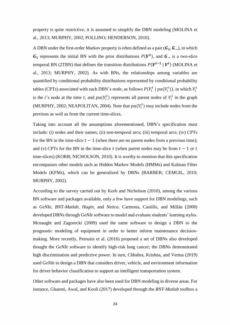
24
property is quite restrictive, it is assumed to simplify the DBN modeling (MOLINA et
al., 2013; MURPHY, 2002; POLLINO; HENDERSON, 2010).
A DBN under the first-order Markov property is often defined as a pair (𝑮𝟏, 𝑮→), in which
𝑮𝟏 represents the initial BN with the prior distributions 𝑃(𝑽𝟏), and 𝑮→ is a two-slice
temporal BN (2TBN) that defines the transition distributions 𝑃(𝑽𝒕−𝟏 | 𝑽𝒕) (MOLINA et
al., 2013; MURPHY, 2002). As with BNs, the relationships among variables are
quantified by conditional probability distributions represented by conditional probability
tables (CPTs) associated with each DBN’s node, as follows 𝑃(𝑉𝑖𝑡 | 𝑝𝑎(𝑉𝑖
𝑡)), in which 𝑉𝑖𝑡
is the 𝑖’s node at the time 𝑡, and 𝑝𝑎(𝑉𝑖𝑡) represents all parent nodes of 𝑉𝑖
𝑡 in the graph
(MURPHY, 2002; NEAPOLITAN, 2004). Note that 𝑝𝑎(𝑉𝑖𝑡) may include nodes from the
previous as well as from the current time-slices.
Taking into account all the assumptions aforementioned, DBN’s specification must
include: (i) nodes and their names; (ii) non-temporal arcs; (iii) temporal arcs; (iv) CPTs
for the BN in the time-slice 𝑡 − 1 (when there are no parent nodes from a previous time);
and (v) CPTs for the BN in the time-slice 𝑡 (when parent nodes may be from 𝑡 − 1 or 𝑡
time-slices) (KORB; NICHOLSON, 2010). It is worthy to mention that this specification
encompasses other models such as Hidden Markov Models (HMMs) and Kalman Filter
Models (KFMs), which can be generalized by DBNs (BARBER; CEMGIL, 2010;
MURPHY, 2002).
According to the survey carried out by Korb and Nicholson (2010), among the various
BN software and packages available, only a few have support for DBN modelings, such
as GeNIe, BNT-Matlab, Hugin, and Netica. Carmona, Castillo, and Millán (2008)
developed DBNs through GeNIe software to model and evaluate students’ learning styles.
Mcnaught and Zagorecki (2009) used the same software to design a DBN to the
prognostic modeling of equipment in order to better inform maintenance decision-
making. More recently, Petousis et al. (2016) proposed a set of DBNs also developed
thought the GeNIe software to identify high-risk lung cancer; the DBNs demonstrated
high discrimination and predictive power. In turn, Chhabra, Krishna, and Verma (2019)
used GeNIe to design a DBN that considers driver, vehicle, and environment information
for driver behavior classification to support an intelligent transportation system.
Other software and packages have also been used for DBN modeling in diverse areas. For
instance, Ghanmi, Awal, and Kooli (2017) developed through the BNT-Matlab toolbox a
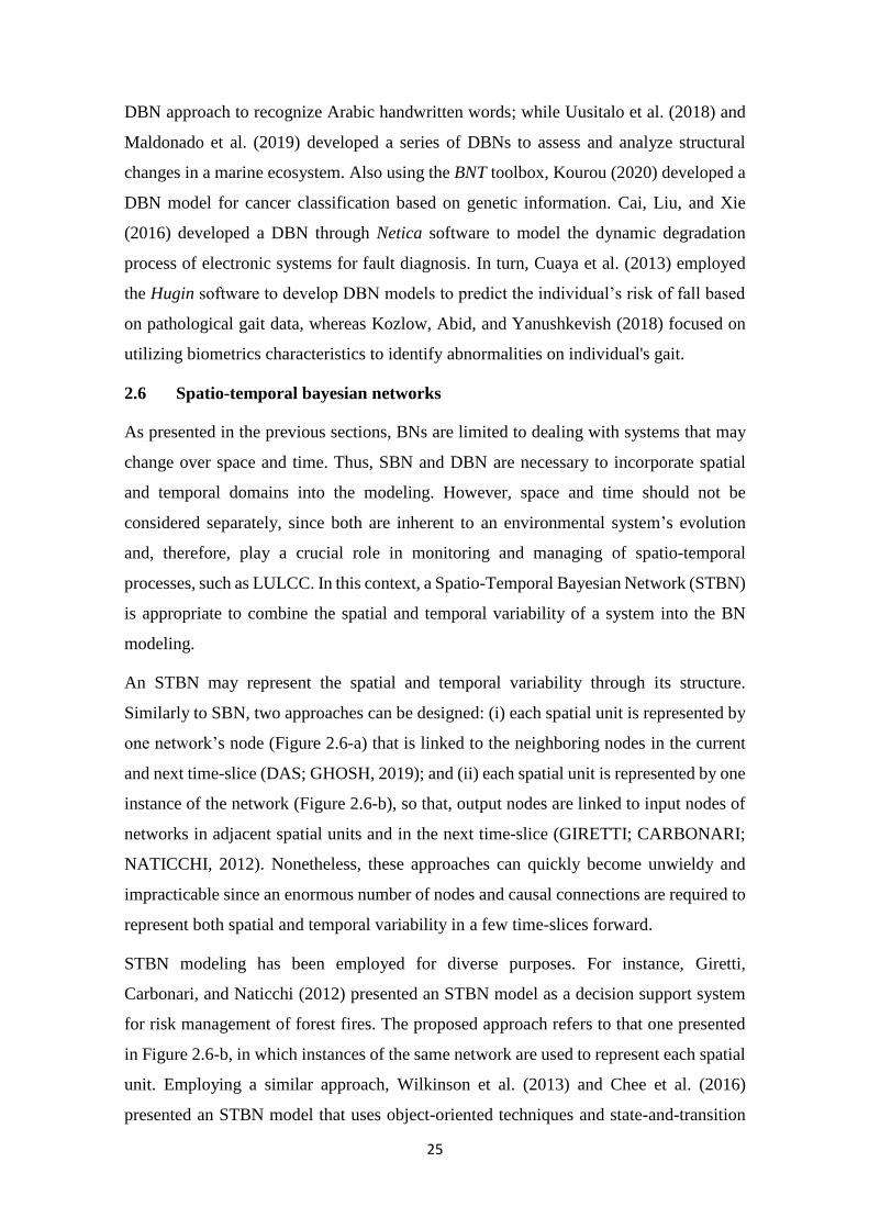
25
DBN approach to recognize Arabic handwritten words; while Uusitalo et al. (2018) and
Maldonado et al. (2019) developed a series of DBNs to assess and analyze structural
changes in a marine ecosystem. Also using the BNT toolbox, Kourou (2020) developed a
DBN model for cancer classification based on genetic information. Cai, Liu, and Xie
(2016) developed a DBN through Netica software to model the dynamic degradation
process of electronic systems for fault diagnosis. In turn, Cuaya et al. (2013) employed
the Hugin software to develop DBN models to predict the individual’s risk of fall based
on pathological gait data, whereas Kozlow, Abid, and Yanushkevish (2018) focused on
utilizing biometrics characteristics to identify abnormalities on individual's gait.
2.6 Spatio-temporal bayesian networks
As presented in the previous sections, BNs are limited to dealing with systems that may
change over space and time. Thus, SBN and DBN are necessary to incorporate spatial
and temporal domains into the modeling. However, space and time should not be
considered separately, since both are inherent to an environmental system’s evolution
and, therefore, play a crucial role in monitoring and managing of spatio-temporal
processes, such as LULCC. In this context, a Spatio-Temporal Bayesian Network (STBN)
is appropriate to combine the spatial and temporal variability of a system into the BN
modeling.
An STBN may represent the spatial and temporal variability through its structure.
Similarly to SBN, two approaches can be designed: (i) each spatial unit is represented by
one network’s node (Figure 2.6-a) that is linked to the neighboring nodes in the current
and next time-slice (DAS; GHOSH, 2019); and (ii) each spatial unit is represented by one
instance of the network (Figure 2.6-b), so that, output nodes are linked to input nodes of
networks in adjacent spatial units and in the next time-slice (GIRETTI; CARBONARI;
NATICCHI, 2012). Nonetheless, these approaches can quickly become unwieldy and
impracticable since an enormous number of nodes and causal connections are required to
represent both spatial and temporal variability in a few time-slices forward.
STBN modeling has been employed for diverse purposes. For instance, Giretti,
Carbonari, and Naticchi (2012) presented an STBN model as a decision support system
for risk management of forest fires. The proposed approach refers to that one presented
in Figure 2.6-b, in which instances of the same network are used to represent each spatial
unit. Employing a similar approach, Wilkinson et al. (2013) and Chee et al. (2016)
presented an STBN model that uses object-oriented techniques and state-and-transition
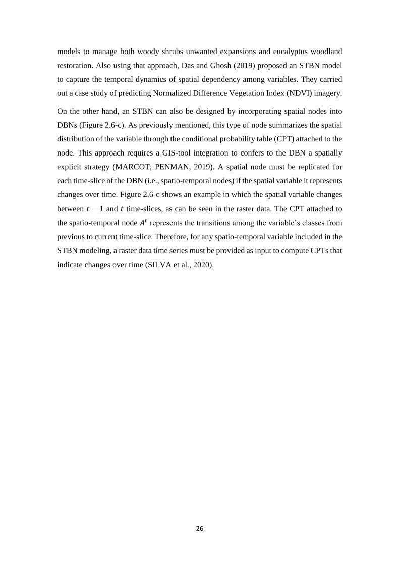
26
models to manage both woody shrubs unwanted expansions and eucalyptus woodland
restoration. Also using that approach, Das and Ghosh (2019) proposed an STBN model
to capture the temporal dynamics of spatial dependency among variables. They carried
out a case study of predicting Normalized Difference Vegetation Index (NDVI) imagery.
On the other hand, an STBN can also be designed by incorporating spatial nodes into
DBNs (Figure 2.6-c). As previously mentioned, this type of node summarizes the spatial
distribution of the variable through the conditional probability table (CPT) attached to the
node. This approach requires a GIS-tool integration to confers to the DBN a spatially
explicit strategy (MARCOT; PENMAN, 2019). A spatial node must be replicated for
each time-slice of the DBN (i.e., spatio-temporal nodes) if the spatial variable it represents
changes over time. Figure 2.6-c shows an example in which the spatial variable changes
between 𝑡 − 1 and 𝑡 time-slices, as can be seen in the raster data. The CPT attached to
the spatio-temporal node 𝐴𝑡 represents the transitions among the variable’s classes from
previous to current time-slice. Therefore, for any spatio-temporal variable included in the
STBN modeling, a raster data time series must be provided as input to compute CPTs that
indicate changes over time (SILVA et al., 2020).
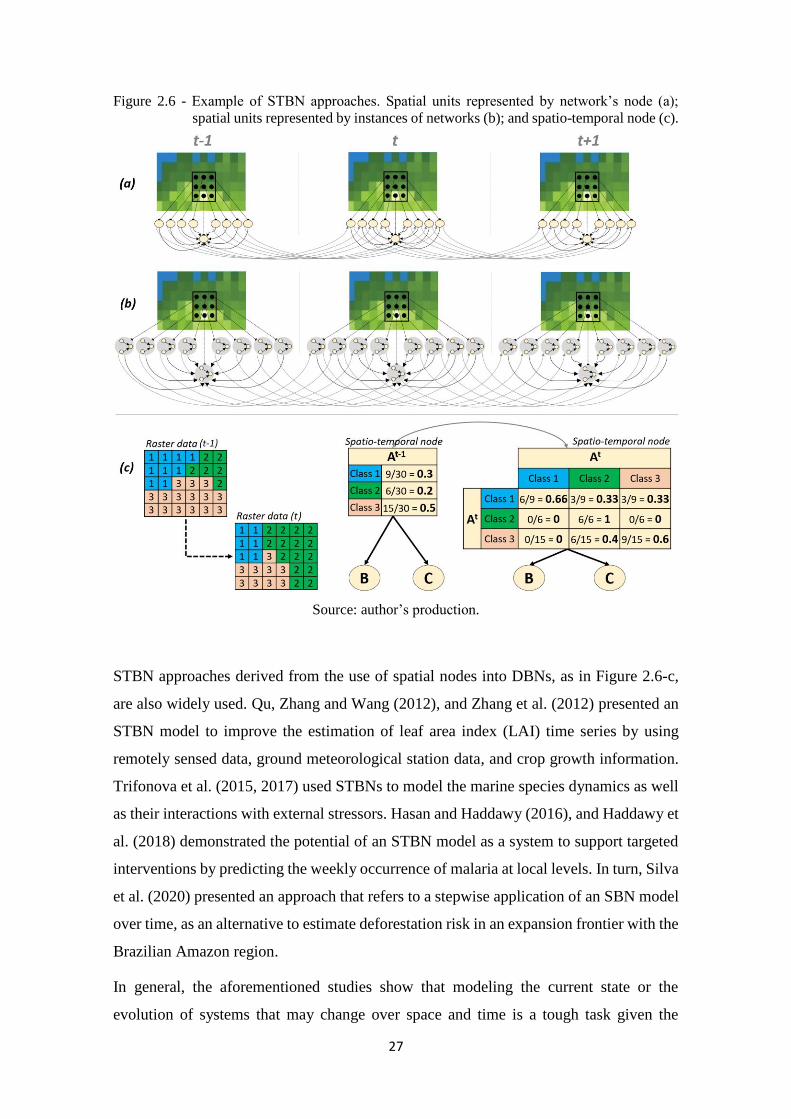
27
Figure 2.6 - Example of STBN approaches. Spatial units represented by network’s node (a);
spatial units represented by instances of networks (b); and spatio-temporal node (c).
Source: author’s production.
STBN approaches derived from the use of spatial nodes into DBNs, as in Figure 2.6-c,
are also widely used. Qu, Zhang and Wang (2012), and Zhang et al. (2012) presented an
STBN model to improve the estimation of leaf area index (LAI) time series by using
remotely sensed data, ground meteorological station data, and crop growth information.
Trifonova et al. (2015, 2017) used STBNs to model the marine species dynamics as well
as their interactions with external stressors. Hasan and Haddawy (2016), and Haddawy et
al. (2018) demonstrated the potential of an STBN model as a system to support targeted
interventions by predicting the weekly occurrence of malaria at local levels. In turn, Silva
et al. (2020) presented an approach that refers to a stepwise application of an SBN model
over time, as an alternative to estimate deforestation risk in an expansion frontier with the
Brazilian Amazon region.
In general, the aforementioned studies show that modeling the current state or the
evolution of systems that may change over space and time is a tough task given the
28
various uncertainties involved. As an STBN model can perform probabilistic reasonings
considering both the spatial and temporal domains, it seems to be an appropriate approach
to estimate LULCC, particularly deforestation risk. Apply BNs to predict deforestation
risk is not unprecedented (DLAMINI, 2016; KRÜGER; LAKES, 2015; MAYFIELD et
al., 2017). However, deforestation has been considered as a static process when modeled
by BNs, which means no time information has been incorporated into the modeling. In
this context, the STBN models developed in this thesis can be readily used to predict
deforestation risk taking into account both space and time information.
29
3. SPATIO-TEMPORAL BAYESIAN NETWORK FOR R (stbnR)
Including spatio-temporal information into the BN model presents some challenges.
Several works that employ Spatial BNs (SBNs) or Spatio-Temporal BN (STBNs) use at
least two different tools to perform the complete analysis: a BN software to build the
network structure and carry out Bayesian analysis, in addition to GIS that provides
necessary functions for spatial data collection, management, and storage (STEINIGER;
HAY, 2009). Although efforts have already been made to BN-GIS integration
(LANDUYT et al., 2015), the use of two different tools can bring up challenges such as
the integration, transfer, and conversion of data from one tool to another.
Therefore, a framework capable of integrating all the steps to perform STBN modeling
into a single environment seems to be a great demand. In this context, the contribution of
this thesis is the implementation of a package for R programming language named stbnR
(Spatio-Temporal Bayesian Network for R), which enables complete STBN modeling
within the R environment. This package integrates other ones already available for R
language that specifically deal with either spatial and spatio-temporal data manipulation
or BN analysis and inference. Hence, the stbnR package enables the development of
STBN-based models for any phenomenon that has some spatio-temporal variation and/or
is influenced by some spatio-temporal variable.
R is free software and programming language (R CORE TEAM, 2019) that provides a
consistent working environment for statistical computing and analysis. Packages are
fundamental units of reproducible R code that increase the power of R by improving
existing base R functionalities or by adding new ones. For instance, the raster package
(HIJMANS et al., 2019) is for gridded spatial data manipulation and analysis, while the
gRain package (HØJSGAARD, 2012, 2019) handles with analysis and inference of
categorical BNs. Both raster and gRain packages were the basis for the stbnR package
development.
In addition to those, special attention should be given to the bnspatial package
(MASANTE, 2019) as it is directly related to the work developed in this thesis. This
package also integrates functions from both raster and gRain packages to enable the
development of SBN models, employing the spatial node concept (as represented in
Figure 2.3-c). Hence, the bnspatial package provides the necessary functions for a
complete SBN modeling in R. On the other hand, there seem to be no available options
for STBN modeling.
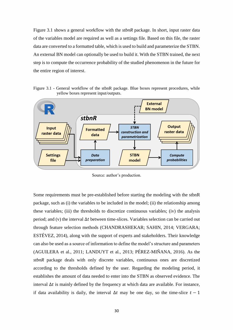
30
Figure 3.1 shows a general workflow with the stbnR package. In short, input raster data
of the variables model are required as well as a settings file. Based on this file, the raster
data are converted to a formatted table, which is used to build and parameterize the STBN.
An external BN model can optionally be used to build it. With the STBN trained, the next
step is to compute the occurrence probability of the studied phenomenon in the future for
the entire region of interest.
Figure 3.1 - General workflow of the stbnR package. Blue boxes represent procedures, while
yellow boxes represent input/outputs.
Source: author’s production.
Some requirements must be pre-established before starting the modeling with the stbnR
package, such as (i) the variables to be included in the model; (ii) the relationship among
these variables; (iii) the thresholds to discretize continuous variables; (iv) the analysis
period; and (v) the interval ∆𝑡 between time-slices. Variables selection can be carried out
through feature selection methods (CHANDRASHEKAR; SAHIN, 2014; VERGARA;
ESTÉVEZ, 2014), along with the support of experts and stakeholders. Their knowledge
can also be used as a source of information to define the model’s structure and parameters
(AGUILERA et al., 2011; LANDUYT et al., 2013; PÉREZ-MIÑANA, 2016). As the
stbnR package deals with only discrete variables, continuous ones are discretized
according to the thresholds defined by the user. Regarding the modeling period, it
establishes the amount of data needed to enter into the STBN as observed evidence. The
interval ∆𝑡 is mainly defined by the frequency at which data are available. For instance,
if data availability is daily, the interval ∆𝑡 may be one day, so the time-slice 𝑡 − 1
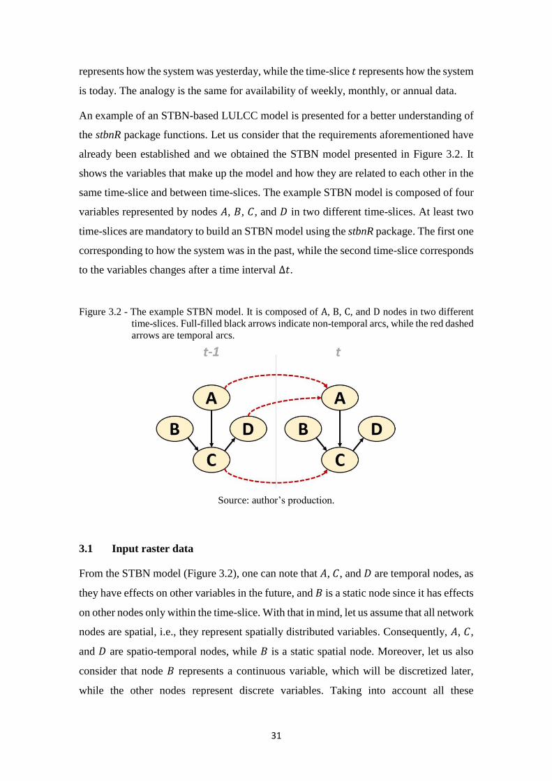
31
represents how the system was yesterday, while the time-slice 𝑡 represents how the system
is today. The analogy is the same for availability of weekly, monthly, or annual data.
An example of an STBN-based LULCC model is presented for a better understanding of
the stbnR package functions. Let us consider that the requirements aforementioned have
already been established and we obtained the STBN model presented in Figure 3.2. It
shows the variables that make up the model and how they are related to each other in the
same time-slice and between time-slices. The example STBN model is composed of four
variables represented by nodes 𝐴, 𝐵, 𝐶, and 𝐷 in two different time-slices. At least two
time-slices are mandatory to build an STBN model using the stbnR package. The first one
corresponding to how the system was in the past, while the second time-slice corresponds
to the variables changes after a time interval ∆𝑡.
Figure 3.2 - The example STBN model. It is composed of A, B, C, and D nodes in two different
time-slices. Full-filled black arrows indicate non-temporal arcs, while the red dashed
arrows are temporal arcs.
Source: author’s production.
3.1 Input raster data
From the STBN model (Figure 3.2), one can note that 𝐴, 𝐶, and 𝐷 are temporal nodes, as
they have effects on other variables in the future, and 𝐵 is a static node since it has effects
on other nodes only within the time-slice. With that in mind, let us assume that all network
nodes are spatial, i.e., they represent spatially distributed variables. Consequently, 𝐴, 𝐶,
and 𝐷 are spatio-temporal nodes, while 𝐵 is a static spatial node. Moreover, let us also
consider that node 𝐵 represents a continuous variable, which will be discretized later,
while the other nodes represent discrete variables. Taking into account all these
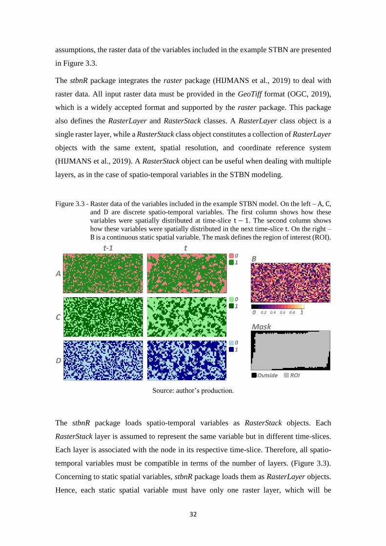
32
assumptions, the raster data of the variables included in the example STBN are presented
in Figure 3.3.
The stbnR package integrates the raster package (HIJMANS et al., 2019) to deal with
raster data. All input raster data must be provided in the GeoTiff format (OGC, 2019),
which is a widely accepted format and supported by the raster package. This package
also defines the RasterLayer and RasterStack classes. A RasterLayer class object is a
single raster layer, while a RasterStack class object constitutes a collection of RasterLayer
objects with the same extent, spatial resolution, and coordinate reference system
(HIJMANS et al., 2019). A RasterStack object can be useful when dealing with multiple
layers, as in the case of spatio-temporal variables in the STBN modeling.
Figure 3.3 - Raster data of the variables included in the example STBN model. On the left – A, C,
and D are discrete spatio-temporal variables. The first column shows how these
variables were spatially distributed at time-slice t − 1. The second column shows
how these variables were spatially distributed in the next time-slice t. On the right –
B is a continuous static spatial variable. The mask defines the region of interest (ROI).
Source: author’s production.
The stbnR package loads spatio-temporal variables as RasterStack objects. Each
RasterStack layer is assumed to represent the same variable but in different time-slices.
Each layer is associated with the node in its respective time-slice. Therefore, all spatio-
temporal variables must be compatible in terms of the number of layers. (Figure 3.3).
Concerning to static spatial variables, stbnR package loads them as RasterLayer objects.
Hence, each static spatial variable must have only one raster layer, which will be
33
replicated to all time-slices. It is important to mention that the stbnR package
distinguishes the variables between temporal or static according to the number of layers.
Therefore, spatio-temporal variables must have two or more raster layers, while static
spatial variables must have only one.
As not all pixels in the entire geographic area may be of interest, the user can provide a
mask as an input raster layer to specify the region of interest (ROI), as presented in Figure
3.3. Only pixels within the ROI will be considered in the analysis, and results will be
calculated only for these pixels. This can bring a significant gain in processing time.
Additionally, the coordinates of the pixels within the ROI will be used as a reference to
observe/collect the values from the other input raster data. Because of this, input raster
data with different spatial resolutions are allowed, saving some data pre-processing time.
The proposal of using a mask to define the ROI is based on the bnspatial package
(MASANTE, 2019). In Figure 3.3, the gray region in the mask represents the ROI, while
the black region represents the area of no interest.
If a mask is provided, its bounding box and spatial resolution will be inherited by the
output raster data. However, if the user does not provide a mask, output raster data inherit
the finest resolution of the input raster data and the maximum extent that encloses all of
them. Besides that, results are calculated for all pixels within the outlined bounding box.
Therefore, it is strongly recommended to provide a mask, otherwise, huge output raster
data can be created, once the stbnR package allows input raster data to have different
extents and spatial resolutions. The only requirement is all of them have the same
coordinate reference system.
3.2 Settings file
Once defined the variables to be included in the model, the user must prepare the settings
file, which is used to format a table according to the Raster*3 objects. The settings file is
a text file (.txt) and must contain some specifications for those nodes that will be
associated with a Raster* objects. The text has to be formatted as follows: (i) the first line
specifies the node name, (ii) the second line lists the node states, and (iii) the third line
enumerates the values from the Raster* object to be associated to the node states; such
values will be integers for discrete data or thresholds of each interval to discretize
3 Raster* refers to RasterLayer or RasterStack.
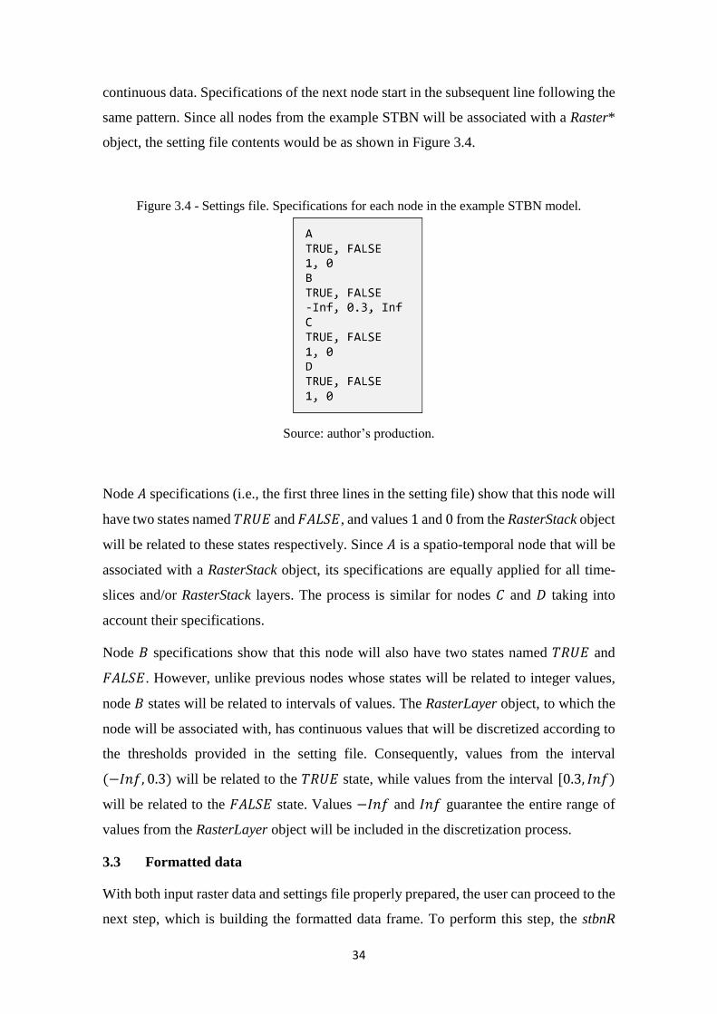
34
continuous data. Specifications of the next node start in the subsequent line following the
same pattern. Since all nodes from the example STBN will be associated with a Raster*
object, the setting file contents would be as shown in Figure 3.4.
Figure 3.4 - Settings file. Specifications for each node in the example STBN model.
Source: author’s production.
Node 𝐴 specifications (i.e., the first three lines in the setting file) show that this node will
have two states named 𝑇𝑅𝑈𝐸 and 𝐹𝐴𝐿𝑆𝐸, and values 1 and 0 from the RasterStack object
will be related to these states respectively. Since 𝐴 is a spatio-temporal node that will be
associated with a RasterStack object, its specifications are equally applied for all time-
slices and/or RasterStack layers. The process is similar for nodes 𝐶 and 𝐷 taking into
account their specifications.
Node 𝐵 specifications show that this node will also have two states named 𝑇𝑅𝑈𝐸 and
𝐹𝐴𝐿𝑆𝐸. However, unlike previous nodes whose states will be related to integer values,
node 𝐵 states will be related to intervals of values. The RasterLayer object, to which the
node will be associated with, has continuous values that will be discretized according to
the thresholds provided in the setting file. Consequently, values from the interval
(−𝐼𝑛𝑓, 0.3) will be related to the 𝑇𝑅𝑈𝐸 state, while values from the interval [0.3, 𝐼𝑛𝑓)
will be related to the 𝐹𝐴𝐿𝑆𝐸 state. Values −𝐼𝑛𝑓 and 𝐼𝑛𝑓 guarantee the entire range of
values from the RasterLayer object will be included in the discretization process.
3.3 Formatted data
With both input raster data and settings file properly prepared, the user can proceed to the
next step, which is building the formatted data frame. To perform this step, the stbnR
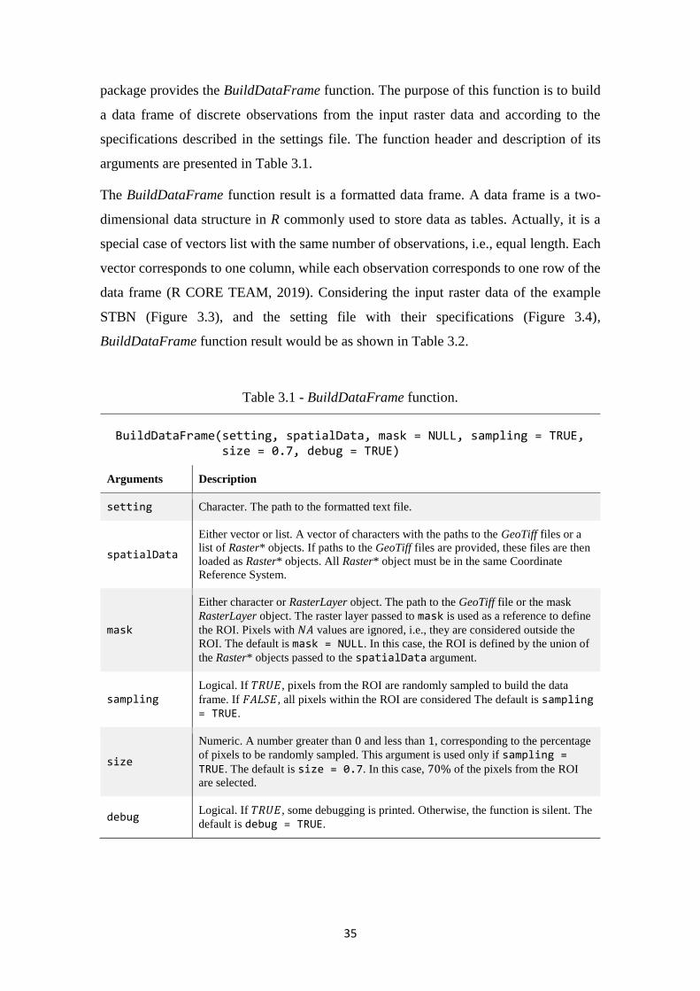
35
package provides the BuildDataFrame function. The purpose of this function is to build
a data frame of discrete observations from the input raster data and according to the
specifications described in the settings file. The function header and description of its
arguments are presented in Table 3.1.
The BuildDataFrame function result is a formatted data frame. A data frame is a two-
dimensional data structure in R commonly used to store data as tables. Actually, it is a
special case of vectors list with the same number of observations, i.e., equal length. Each
vector corresponds to one column, while each observation corresponds to one row of the
data frame (R CORE TEAM, 2019). Considering the input raster data of the example
STBN (Figure 3.3), and the setting file with their specifications (Figure 3.4),
BuildDataFrame function result would be as shown in Table 3.2.
Table 3.1 - BuildDataFrame function.
BuildDataFrame(setting, spatialData, mask = NULL, sampling = TRUE, size = 0.7, debug = TRUE)
Arguments Description
setting Character. The path to the formatted text file.
spatialData
Either vector or list. A vector of characters with the paths to the GeoTiff files or a
list of Raster* objects. If paths to the GeoTiff files are provided, these files are then
loaded as Raster* objects. All Raster* object must be in the same Coordinate
Reference System.
mask
Either character or RasterLayer object. The path to the GeoTiff file or the mask
RasterLayer object. The raster layer passed to mask is used as a reference to define
the ROI. Pixels with 𝑁𝐴 values are ignored, i.e., they are considered outside the
ROI. The default is mask = NULL. In this case, the ROI is defined by the union of
the Raster* objects passed to the spatialData argument.
sampling Logical. If 𝑇𝑅𝑈𝐸, pixels from the ROI are randomly sampled to build the data
frame. If 𝐹𝐴𝐿𝑆𝐸, all pixels within the ROI are considered The default is sampling = TRUE.
size
Numeric. A number greater than 0 and less than 1, corresponding to the percentage
of pixels to be randomly sampled. This argument is used only if sampling = TRUE. The default is size = 0.7. In this case, 70% of the pixels from the ROI
are selected.
debug Logical. If 𝑇𝑅𝑈𝐸, some debugging is printed. Otherwise, the function is silent. The
default is debug = TRUE.
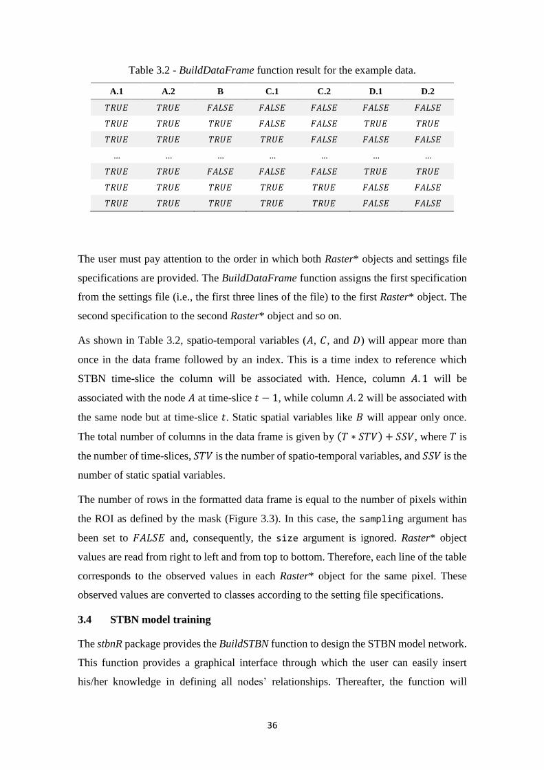
36
Table 3.2 - BuildDataFrame function result for the example data.
A.1 A.2 B C.1 C.2 D.1 D.2
𝑇𝑅𝑈𝐸 𝑇𝑅𝑈𝐸 𝐹𝐴𝐿𝑆𝐸 𝐹𝐴𝐿𝑆𝐸 𝐹𝐴𝐿𝑆𝐸 𝐹𝐴𝐿𝑆𝐸 𝐹𝐴𝐿𝑆𝐸
𝑇𝑅𝑈𝐸 𝑇𝑅𝑈𝐸 𝑇𝑅𝑈𝐸 𝐹𝐴𝐿𝑆𝐸 𝐹𝐴𝐿𝑆𝐸 𝑇𝑅𝑈𝐸 𝑇𝑅𝑈𝐸
𝑇𝑅𝑈𝐸 𝑇𝑅𝑈𝐸 𝑇𝑅𝑈𝐸 𝑇𝑅𝑈𝐸 𝐹𝐴𝐿𝑆𝐸 𝐹𝐴𝐿𝑆𝐸 𝐹𝐴𝐿𝑆𝐸
… … … … … … …
𝑇𝑅𝑈𝐸 𝑇𝑅𝑈𝐸 𝐹𝐴𝐿𝑆𝐸 𝐹𝐴𝐿𝑆𝐸 𝐹𝐴𝐿𝑆𝐸 𝑇𝑅𝑈𝐸 𝑇𝑅𝑈𝐸
𝑇𝑅𝑈𝐸 𝑇𝑅𝑈𝐸 𝑇𝑅𝑈𝐸 𝑇𝑅𝑈𝐸 𝑇𝑅𝑈𝐸 𝐹𝐴𝐿𝑆𝐸 𝐹𝐴𝐿𝑆𝐸
𝑇𝑅𝑈𝐸 𝑇𝑅𝑈𝐸 𝑇𝑅𝑈𝐸 𝑇𝑅𝑈𝐸 𝑇𝑅𝑈𝐸 𝐹𝐴𝐿𝑆𝐸 𝐹𝐴𝐿𝑆𝐸
The user must pay attention to the order in which both Raster* objects and settings file
specifications are provided. The BuildDataFrame function assigns the first specification
from the settings file (i.e., the first three lines of the file) to the first Raster* object. The
second specification to the second Raster* object and so on.
As shown in Table 3.2, spatio-temporal variables (𝐴, 𝐶, and 𝐷) will appear more than
once in the data frame followed by an index. This is a time index to reference which
STBN time-slice the column will be associated with. Hence, column 𝐴. 1 will be
associated with the node 𝐴 at time-slice 𝑡 − 1, while column 𝐴. 2 will be associated with
the same node but at time-slice 𝑡. Static spatial variables like 𝐵 will appear only once.
The total number of columns in the data frame is given by (𝑇 ∗ 𝑆𝑇𝑉) + 𝑆𝑆𝑉, where 𝑇 is
the number of time-slices, 𝑆𝑇𝑉 is the number of spatio-temporal variables, and 𝑆𝑆𝑉 is the
number of static spatial variables.
The number of rows in the formatted data frame is equal to the number of pixels within
the ROI as defined by the mask (Figure 3.3). In this case, the sampling argument has
been set to 𝐹𝐴𝐿𝑆𝐸 and, consequently, the size argument is ignored. Raster* object
values are read from right to left and from top to bottom. Therefore, each line of the table
corresponds to the observed values in each Raster* object for the same pixel. These
observed values are converted to classes according to the setting file specifications.
3.4 STBN model training
The stbnR package provides the BuildSTBN function to design the STBN model network.
This function provides a graphical interface through which the user can easily insert
his/her knowledge in defining all nodes’ relationships. Thereafter, the function will
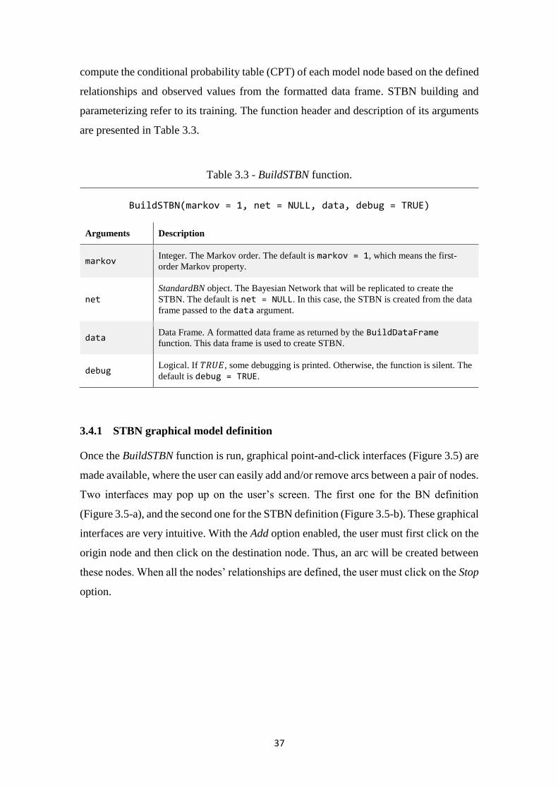
37
compute the conditional probability table (CPT) of each model node based on the defined
relationships and observed values from the formatted data frame. STBN building and
parameterizing refer to its training. The function header and description of its arguments
are presented in Table 3.3.
Table 3.3 - BuildSTBN function.
BuildSTBN(markov = 1, net = NULL, data, debug = TRUE)
Arguments Description
markov Integer. The Markov order. The default is markov = 1, which means the first-
order Markov property.
net StandardBN object. The Bayesian Network that will be replicated to create the
STBN. The default is net = NULL. In this case, the STBN is created from the data
frame passed to the data argument.
data Data Frame. A formatted data frame as returned by the BuildDataFrame
function. This data frame is used to create STBN.
debug Logical. If 𝑇𝑅𝑈𝐸, some debugging is printed. Otherwise, the function is silent. The
default is debug = TRUE.
3.4.1 STBN graphical model definition
Once the BuildSTBN function is run, graphical point-and-click interfaces (Figure 3.5) are
made available, where the user can easily add and/or remove arcs between a pair of nodes.
Two interfaces may pop up on the user’s screen. The first one for the BN definition
(Figure 3.5-a), and the second one for the STBN definition (Figure 3.5-b). These graphical
interfaces are very intuitive. With the Add option enabled, the user must first click on the
origin node and then click on the destination node. Thus, an arc will be created between
these nodes. When all the nodes’ relationships are defined, the user must click on the Stop
option.
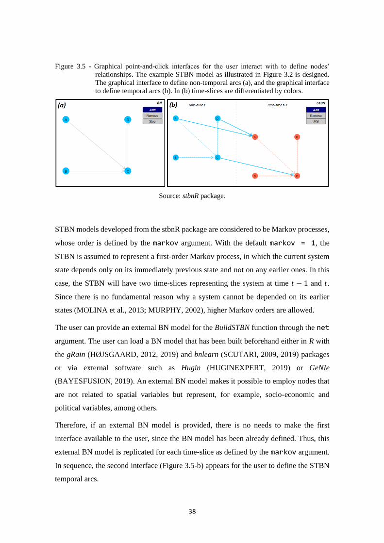
38
Figure 3.5 - Graphical point-and-click interfaces for the user interact with to define nodes’
relationships. The example STBN model as illustrated in Figure 3.2 is designed.
The graphical interface to define non-temporal arcs (a), and the graphical interface
to define temporal arcs (b). In (b) time-slices are differentiated by colors.
Source: stbnR package.
STBN models developed from the stbnR package are considered to be Markov processes,
whose order is defined by the markov argument. With the default markov = 1, the
STBN is assumed to represent a first-order Markov process, in which the current system
state depends only on its immediately previous state and not on any earlier ones. In this
case, the STBN will have two time-slices representing the system at time 𝑡 − 1 and 𝑡.
Since there is no fundamental reason why a system cannot be depended on its earlier
states (MOLINA et al., 2013; MURPHY, 2002), higher Markov orders are allowed.
The user can provide an external BN model for the BuildSTBN function through the net
argument. The user can load a BN model that has been built beforehand either in R with
the gRain (HØJSGAARD, 2012, 2019) and bnlearn (SCUTARI, 2009, 2019) packages
or via external software such as Hugin (HUGINEXPERT, 2019) or GeNIe
(BAYESFUSION, 2019). An external BN model makes it possible to employ nodes that
are not related to spatial variables but represent, for example, socio-economic and
political variables, among others.
Therefore, if an external BN model is provided, there is no needs to make the first
interface available to the user, since the BN model has been already defined. Thus, this
external BN model is replicated for each time-slice as defined by the markov argument.
In sequence, the second interface (Figure 3.5-b) appears for the user to define the STBN
temporal arcs.
39
The user also has the option to build the STBN model from scratch from the formatted
data frame provided through the data argument. The BuildSTBN function will identify
the unique nodes from the data frame columns. Thereafter, the first interface (Figure 3.5-
a) will pop up on the screen, and the user has to define the directed acyclic graph (DAG)
of the BN model. This first interface helps the user not to make mistakes like creating a
cycle in the graph. Whenever an arc closes a cycle, it is promptly ignored.
After finishing the DAG editing, the second interface automatically appears (Figure 3.5-
b), and the user has to define the STBN temporal arcs. Only forward arcs between pairs
of temporal nodes are allowed. This second interface does not allow the user to create
backward temporal arcs, temporal arcs between static nodes, or to edit non-temporal arcs.
Figure 3.5 shows the graphical interfaces to create the example STBN.
3.4.2 Conditional probability tables computation
Once the STNB graphical model is defined, the BuildSTBN function will automatically
compute the CPTs of all network nodes using the observed values in the formatted data
frame. A CPT is calculated from the frequency table, which contains the number of
occurrences of specific observations within a dataset. Probabilities are then calculated
from the ratio between each frequency table entry by the total number of observations.
Let us consider the observed values for the node 𝐷𝑡−1 (i.e., node 𝐷 in the time-slice 𝑡 − 1
of the example STBN model). Figure 3.6-a shows that among all observations of this
node, approximately 42% belong to the 𝑇𝑅𝑈𝐸 state and, therefore, 58% belong to the
𝐹𝐴𝐿𝑆𝐸 state. These values represent what would be the prior probability of the node
𝐷𝑡−1, that is 𝑃(𝐷𝑡−1 = 𝑇𝑅𝑈𝐸) = 0.42 and 𝑃(𝐷𝑡−1 = 𝐹𝐴𝐿𝑆𝐸) = 0.58.
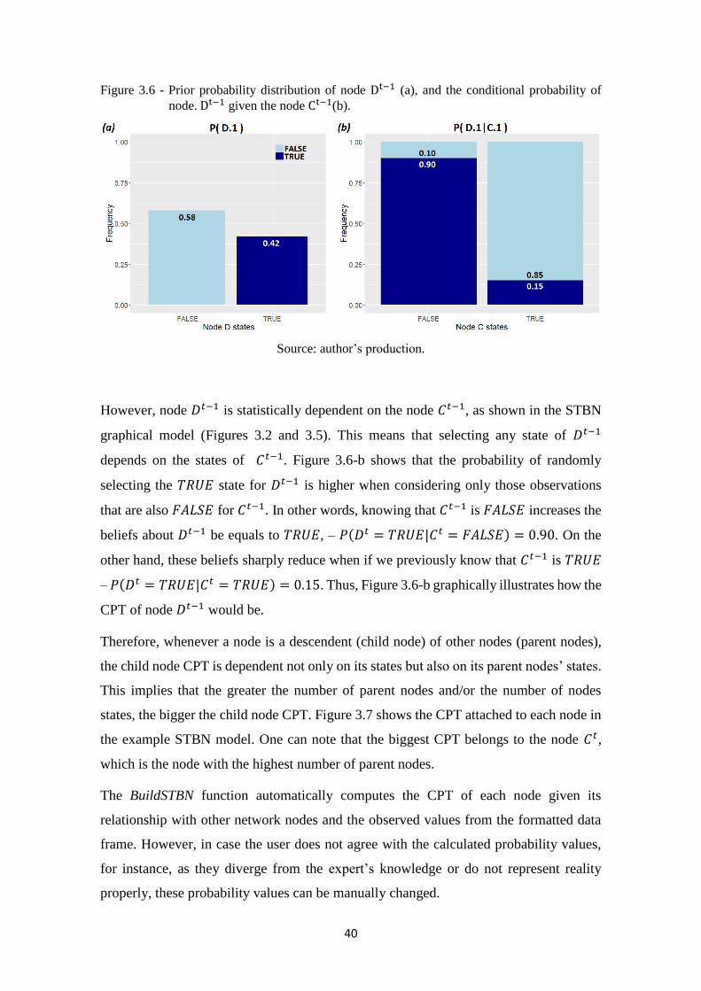
40
Figure 3.6 - Prior probability distribution of node Dt−1 (a), and the conditional probability of
node. Dt−1 given the node Ct−1(b).
Source: author’s production.
However, node 𝐷𝑡−1 is statistically dependent on the node 𝐶𝑡−1, as shown in the STBN
graphical model (Figures 3.2 and 3.5). This means that selecting any state of 𝐷𝑡−1
depends on the states of 𝐶𝑡−1. Figure 3.6-b shows that the probability of randomly
selecting the 𝑇𝑅𝑈𝐸 state for 𝐷𝑡−1 is higher when considering only those observations
that are also 𝐹𝐴𝐿𝑆𝐸 for 𝐶𝑡−1. In other words, knowing that 𝐶𝑡−1 is 𝐹𝐴𝐿𝑆𝐸 increases the
beliefs about 𝐷𝑡−1 be equals to 𝑇𝑅𝑈𝐸, – 𝑃(𝐷𝑡 = 𝑇𝑅𝑈𝐸|𝐶𝑡 = 𝐹𝐴𝐿𝑆𝐸) = 0.90. On the
other hand, these beliefs sharply reduce when if we previously know that 𝐶𝑡−1 is 𝑇𝑅𝑈𝐸
– 𝑃(𝐷𝑡 = 𝑇𝑅𝑈𝐸|𝐶𝑡 = 𝑇𝑅𝑈𝐸) = 0.15. Thus, Figure 3.6-b graphically illustrates how the
CPT of node 𝐷𝑡−1 would be.
Therefore, whenever a node is a descendent (child node) of other nodes (parent nodes),
the child node CPT is dependent not only on its states but also on its parent nodes’ states.
This implies that the greater the number of parent nodes and/or the number of nodes
states, the bigger the child node CPT. Figure 3.7 shows the CPT attached to each node in
the example STBN model. One can note that the biggest CPT belongs to the node 𝐶𝑡,
which is the node with the highest number of parent nodes.
The BuildSTBN function automatically computes the CPT of each node given its
relationship with other network nodes and the observed values from the formatted data
frame. However, in case the user does not agree with the calculated probability values,
for instance, as they diverge from the expert’s knowledge or do not represent reality
properly, these probability values can be manually changed.
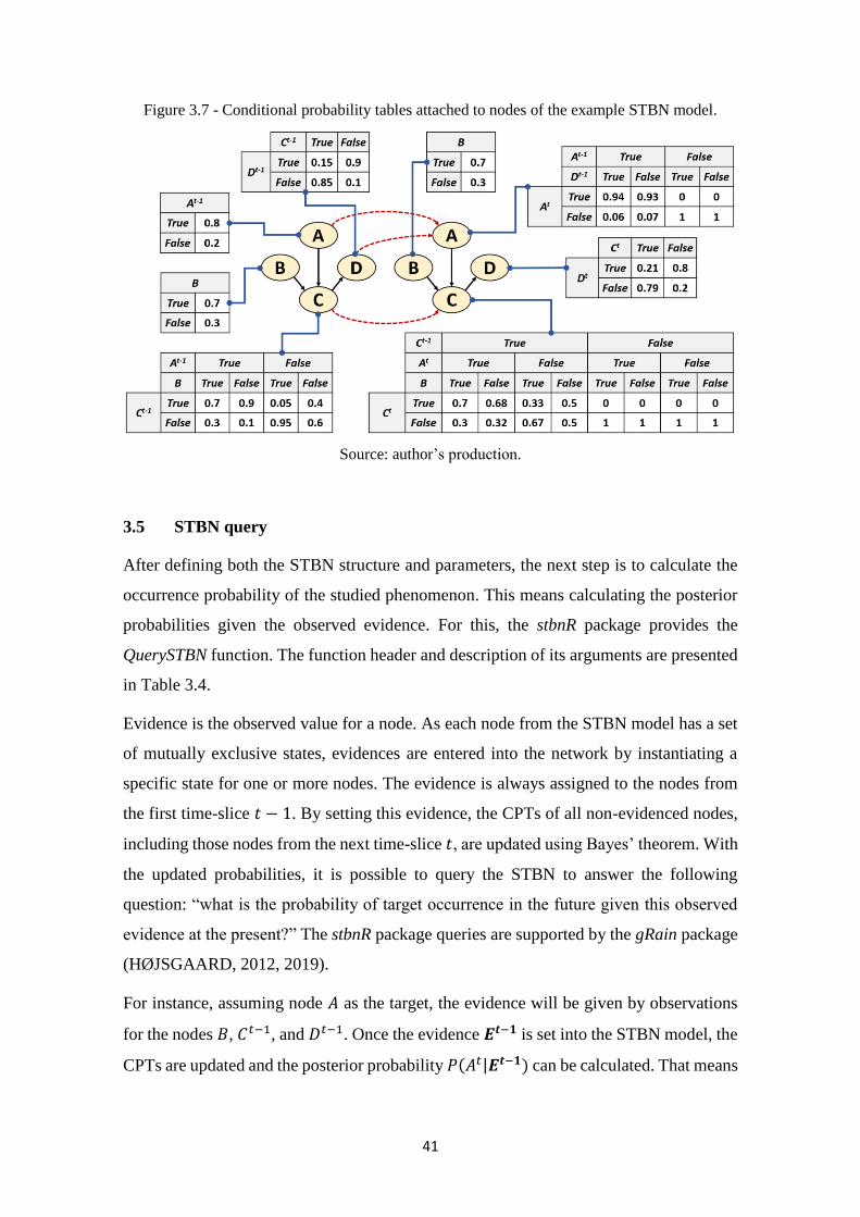
41
Figure 3.7 - Conditional probability tables attached to nodes of the example STBN model.
Source: author’s production.
3.5 STBN query
After defining both the STBN structure and parameters, the next step is to calculate the
occurrence probability of the studied phenomenon. This means calculating the posterior
probabilities given the observed evidence. For this, the stbnR package provides the
QuerySTBN function. The function header and description of its arguments are presented
in Table 3.4.
Evidence is the observed value for a node. As each node from the STBN model has a set
of mutually exclusive states, evidences are entered into the network by instantiating a
specific state for one or more nodes. The evidence is always assigned to the nodes from
the first time-slice 𝑡 − 1. By setting this evidence, the CPTs of all non-evidenced nodes,
including those nodes from the next time-slice 𝑡, are updated using Bayes’ theorem. With
the updated probabilities, it is possible to query the STBN to answer the following
question: “what is the probability of target occurrence in the future given this observed
evidence at the present?” The stbnR package queries are supported by the gRain package
(HØJSGAARD, 2012, 2019).
For instance, assuming node 𝐴 as the target, the evidence will be given by observations
for the nodes 𝐵, 𝐶𝑡−1, and 𝐷𝑡−1. Once the evidence 𝑬𝒕−𝟏 is set into the STBN model, the
CPTs are updated and the posterior probability 𝑃(𝐴𝑡|𝑬𝒕−𝟏) can be calculated. That means
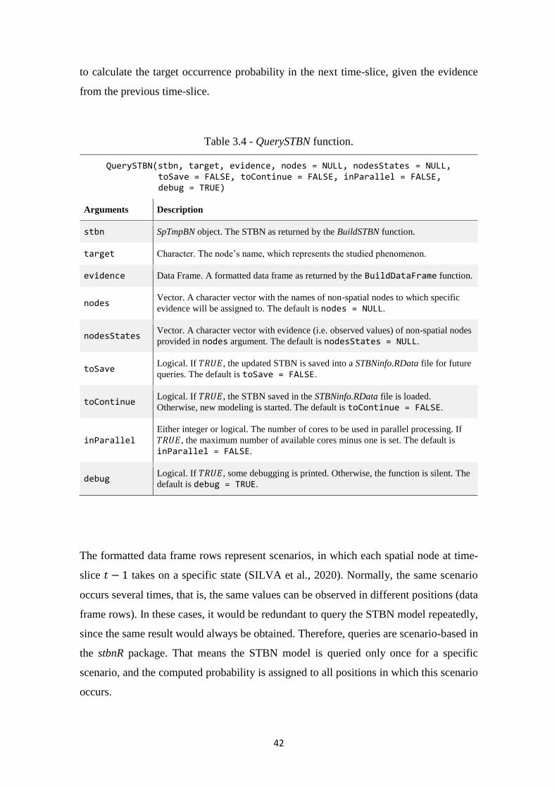
42
to calculate the target occurrence probability in the next time-slice, given the evidence
from the previous time-slice.
Table 3.4 - QuerySTBN function.
QuerySTBN(stbn, target, evidence, nodes = NULL, nodesStates = NULL, toSave = FALSE, toContinue = FALSE, inParallel = FALSE, debug = TRUE)
Arguments Description
stbn SpTmpBN object. The STBN as returned by the BuildSTBN function.
target Character. The node’s name, which represents the studied phenomenon.
evidence Data Frame. A formatted data frame as returned by the BuildDataFrame function.
nodes Vector. A character vector with the names of non-spatial nodes to which specific
evidence will be assigned to. The default is nodes = NULL.
nodesStates Vector. A character vector with evidence (i.e. observed values) of non-spatial nodes
provided in nodes argument. The default is nodesStates = NULL.
toSave Logical. If 𝑇𝑅𝑈𝐸, the updated STBN is saved into a STBNinfo.RData file for future
queries. The default is toSave = FALSE.
toContinue Logical. If 𝑇𝑅𝑈𝐸, the STBN saved in the STBNinfo.RData file is loaded.
Otherwise, new modeling is started. The default is toContinue = FALSE.
inParallel Either integer or logical. The number of cores to be used in parallel processing. If
𝑇𝑅𝑈𝐸, the maximum number of available cores minus one is set. The default is
inParallel = FALSE.
debug Logical. If 𝑇𝑅𝑈𝐸, some debugging is printed. Otherwise, the function is silent. The
default is debug = TRUE.
The formatted data frame rows represent scenarios, in which each spatial node at time-
slice 𝑡 − 1 takes on a specific state (SILVA et al., 2020). Normally, the same scenario
occurs several times, that is, the same values can be observed in different positions (data
frame rows). In these cases, it would be redundant to query the STBN model repeatedly,
since the same result would always be obtained. Therefore, queries are scenario-based in
the stbnR package. That means the STBN model is queried only once for a specific
scenario, and the computed probability is assigned to all positions in which this scenario
occurs.
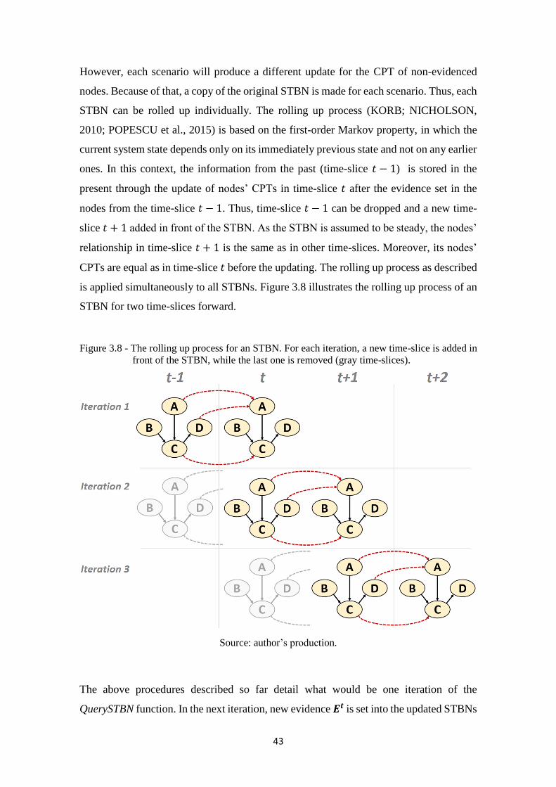
43
However, each scenario will produce a different update for the CPT of non-evidenced
nodes. Because of that, a copy of the original STBN is made for each scenario. Thus, each
STBN can be rolled up individually. The rolling up process (KORB; NICHOLSON,
2010; POPESCU et al., 2015) is based on the first-order Markov property, in which the
current system state depends only on its immediately previous state and not on any earlier
ones. In this context, the information from the past (time-slice 𝑡 − 1) is stored in the
present through the update of nodes’ CPTs in time-slice 𝑡 after the evidence set in the
nodes from the time-slice 𝑡 − 1. Thus, time-slice 𝑡 − 1 can be dropped and a new time-
slice 𝑡 + 1 added in front of the STBN. As the STBN is assumed to be steady, the nodes’
relationship in time-slice 𝑡 + 1 is the same as in other time-slices. Moreover, its nodes’
CPTs are equal as in time-slice 𝑡 before the updating. The rolling up process as described
is applied simultaneously to all STBNs. Figure 3.8 illustrates the rolling up process of an
STBN for two time-slices forward.
Figure 3.8 - The rolling up process for an STBN. For each iteration, a new time-slice is added in
front of the STBN, while the last one is removed (gray time-slices).
Source: author’s production.
The above procedures described so far detail what would be one iteration of the
QuerySTBN function. In the next iteration, new evidence 𝑬𝒕 is set into the updated STBNs
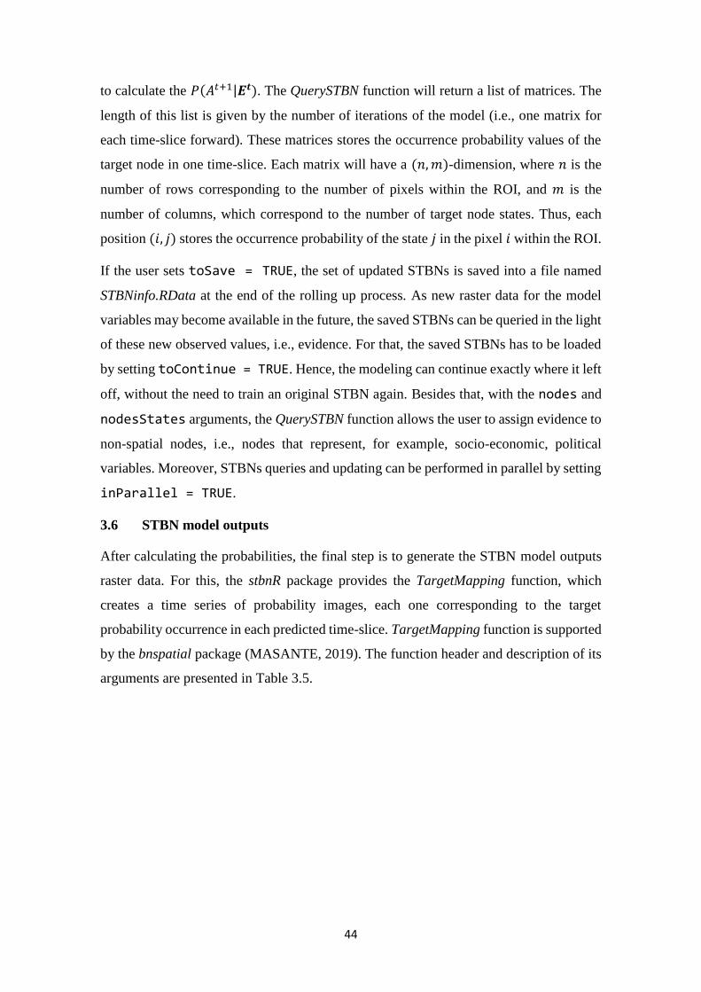
44
to calculate the 𝑃(𝐴𝑡+1|𝑬𝒕). The QuerySTBN function will return a list of matrices. The
length of this list is given by the number of iterations of the model (i.e., one matrix for
each time-slice forward). These matrices stores the occurrence probability values of the
target node in one time-slice. Each matrix will have a (𝑛, 𝑚)-dimension, where 𝑛 is the
number of rows corresponding to the number of pixels within the ROI, and 𝑚 is the
number of columns, which correspond to the number of target node states. Thus, each
position (𝑖, 𝑗) stores the occurrence probability of the state 𝑗 in the pixel 𝑖 within the ROI.
If the user sets toSave = TRUE, the set of updated STBNs is saved into a file named
STBNinfo.RData at the end of the rolling up process. As new raster data for the model
variables may become available in the future, the saved STBNs can be queried in the light
of these new observed values, i.e., evidence. For that, the saved STBNs has to be loaded
by setting toContinue = TRUE. Hence, the modeling can continue exactly where it left
off, without the need to train an original STBN again. Besides that, with the nodes and
nodesStates arguments, the QuerySTBN function allows the user to assign evidence to
non-spatial nodes, i.e., nodes that represent, for example, socio-economic, political
variables. Moreover, STBNs queries and updating can be performed in parallel by setting
inParallel = TRUE.
3.6 STBN model outputs
After calculating the probabilities, the final step is to generate the STBN model outputs
raster data. For this, the stbnR package provides the TargetMapping function, which
creates a time series of probability images, each one corresponding to the target
probability occurrence in each predicted time-slice. TargetMapping function is supported
by the bnspatial package (MASANTE, 2019). The function header and description of its
arguments are presented in Table 3.5.
45
Table 3.5 - TargetMapping function.
TargetMapping(target, probs, what = “probability”, mask, toExport = FALSE, path, debug = TRUE)
Arguments Description
target Character. The node’s name, which represents the studied phenomenon.
probs List. A list of matrixes as returned by the QuerySTBN function.
what Vector. A character vector specifying the required output. The options are (i) class,
which returns the most likely state; (ii) entropy, which returns the Shannon entropy;
and (iii) probability. The default is what = “probability”.
mask
Either character or RasterLayer object. The path to the GeoTiff file or the mask
RasterLayer object. The raster layer passed to mask is used as a reference to define
the ROI. Pixels with 𝑁𝐴 values are ignored, i.e., they are considered outside the
ROI.
toExport Logical. If 𝑇𝑅𝑈𝐸 output raster data are saved as GeoTiff files. The default is
toExport = FALSE.
debug Logical. If 𝑇𝑅𝑈𝐸, some debugging is printed. Otherwise, the function is silent. The
default is debug = TRUE.
The TargetMapping function will return a raster layer for each time-slice rolled up
forward. The results of this function can be changed according to what argument. For
instance, if what = class, the value of each pixel within the ROI will refer to the most
likely target state to occur. With what = entropy, pixel values will refer to the
calculation of Shannon’s entropy, which evaluates the uncertainties of each prediction
(HAMMER et al., 2000). In turn, if what = probability, pixels values will be the
probability values. In this case, a probability image will be generated for each target node
state.
The target node must be the same as the one defined for the QuerySTBN function. The
mask to be provided for the TargetMapping function must be the same as that provided
for the BuildDataFrame function. As mentioned previously, this mask is used as a
reference, its extension and spatial resolution will be inherent by the output raster data.
Finally, the user can save all output raster data as GeoTiff files if toExport = TRUE.
46
4 STBN MODELS FOR DEFORESTATION RISK PREDICTION
This chapter aims to present the application of the STBN models proposed in this work
to predict deforestation risk in some regions of the Brazilian Legal Amazon (BLA).
Although employing BNs as an approach to predict deforestation risk had been proposed
before (DLAMINI, 2016; KRÜGER; LAKES, 2015; MAYFIELD et al., 2017), the
temporal domain has not been considered until then. Therefore deforestation has been
considered as a static process when modeled by BN approaches. In this context, the STBN
models developed from the stbnR package aim to meet this demand, since they enable
incorporating spatial and temporal information into the modeling. Furthermore, with the
case studies presented in this work, we can evaluate the potential of the STBN as a
LULCC model.
4.1 Case study regions
To evaluate the STBN model to predict deforestation risk, three regions of interest (ROIs)
were selected (Figure 4.1) with expert support to encompass different deforestation
frontiers within the BLA. The selected regions are located in the Amazonas, Mato Grosso,
and Pará states. These last two states accumulate more than 60% (480728 𝑘𝑚2) of the
entire deforested area in the BLA (788352.9 𝑘𝑚2) until 2018 (INPE, 2019a). Hence,
Pará and Mato Grosso are respectively the first and second states with the largest
deforested areas. Although Amazonas state occupies the fifth position in this rank, there
is a great concern due to the emergence of a new deforestation expansion frontier. Figure
4.1 also shows deforested areas until 2018 (red-colored) as well as forest areas (green-
colored) within each region (INPE, 2019a). Following, we describe each of these regions.
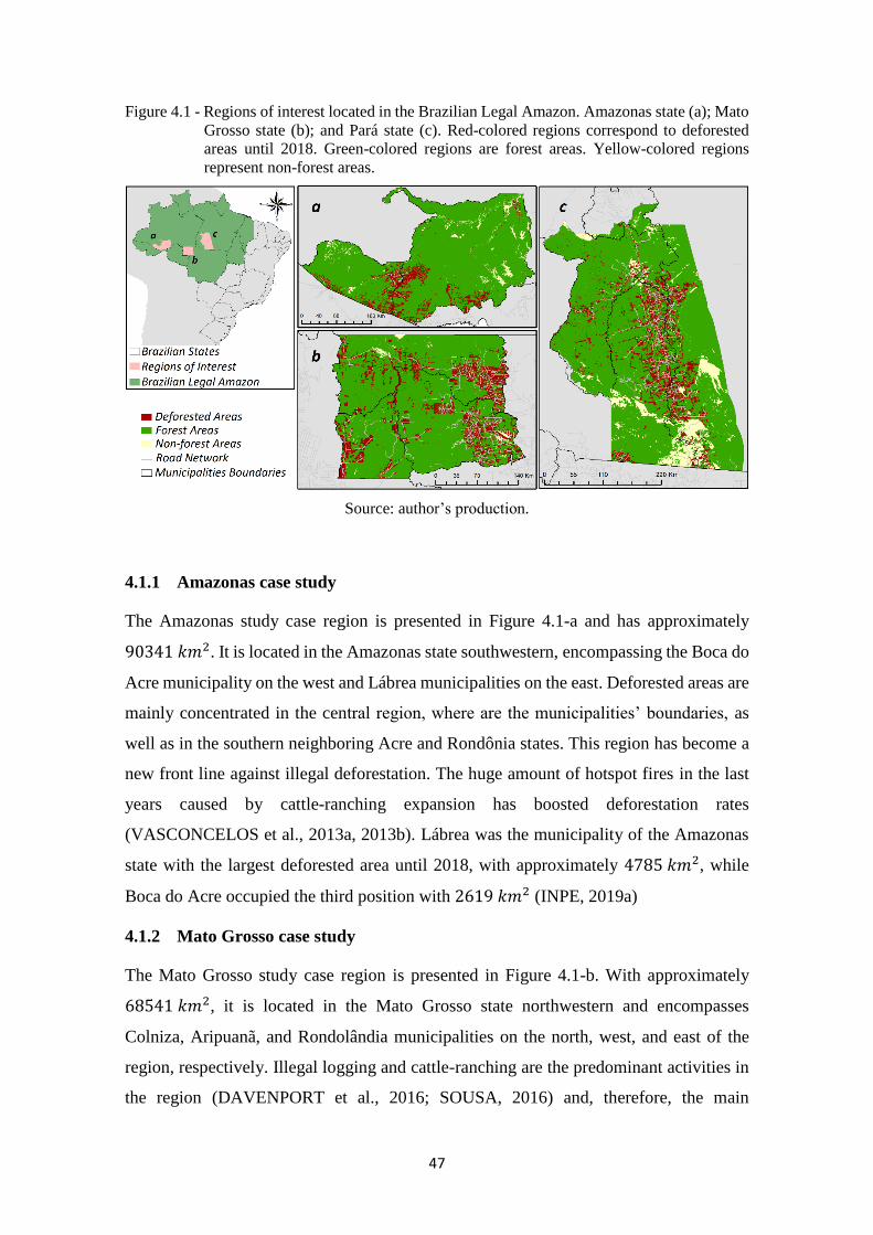
47
Figure 4.1 - Regions of interest located in the Brazilian Legal Amazon. Amazonas state (a); Mato
Grosso state (b); and Pará state (c). Red-colored regions correspond to deforested
areas until 2018. Green-colored regions are forest areas. Yellow-colored regions
represent non-forest areas.
Source: author’s production.
4.1.1 Amazonas case study
The Amazonas study case region is presented in Figure 4.1-a and has approximately
90341 𝑘𝑚2. It is located in the Amazonas state southwestern, encompassing the Boca do
Acre municipality on the west and Lábrea municipalities on the east. Deforested areas are
mainly concentrated in the central region, where are the municipalities’ boundaries, as
well as in the southern neighboring Acre and Rondônia states. This region has become a
new front line against illegal deforestation. The huge amount of hotspot fires in the last
years caused by cattle-ranching expansion has boosted deforestation rates
(VASCONCELOS et al., 2013a, 2013b). Lábrea was the municipality of the Amazonas
state with the largest deforested area until 2018, with approximately 4785 𝑘𝑚2, while
Boca do Acre occupied the third position with 2619 𝑘𝑚2 (INPE, 2019a)
4.1.2 Mato Grosso case study
The Mato Grosso study case region is presented in Figure 4.1-b. With approximately
68541 𝑘𝑚2, it is located in the Mato Grosso state northwestern and encompasses
Colniza, Aripuanã, and Rondolândia municipalities on the north, west, and east of the
region, respectively. Illegal logging and cattle-ranching are the predominant activities in
the region (DAVENPORT et al., 2016; SOUSA, 2016) and, therefore, the main
48
deforestation drivers. Deforested areas can be found throughout the case study region, but
mainly concentrated in the eastern portion. Colniza, Aripuanã, and Rondolândia
municipalities showed the largest deforestation increases in the Mato Grosso state
between 2017-2018. Until this year, deforested areas in Colniza, Aripuanã, and
Rondolândia was 4970 𝑘𝑚2, 4319 𝑘𝑚2, and 2031 𝑘𝑚2, respectively (INPE, 2019a).
4.1.3 Pará case study
The Pará study case region corresponds to a buffer around the BR-163 highway and has
approximately 117138 𝑘𝑚2. The construction of this highway and more recent
improvements in transportation infrastructure have intensified deforestation along its
route over the years (FEARNSIDE, 2007; PINHEIRO et al., 2016), which has created an
expansion deforestation corridor (SILVA et al., 2020), as can be seen in Figure 3.9-c.
Extensive and traditional cattle farming is the main land use in this region (MÜLLER et
al., 2016). The case study region encompasses the Novo Progresso municipality as well
as the southern part of the Altamira and Itaituba municipalities. Until 2018, these
municipalities were among those with the largest extension of deforested areas in the
entire BLA. Novo Progresso municipality, which is completely within the case study
region, had approximately 6289 𝑘𝑚2 of deforested area (INPE, 2019a).
4.2 Dataset and pre-processings
The variables chosen to compose the modeling as well as their pre-processing are detailed
below. All procedures were carried out through the R software (R CORE TEAM, 2019).
The same set of variables was used in three case studies. Therefore, all the procedures
described here were equally applied in all case studies.
The target variable named deforestation represents yearly deforested areas, therefore, it
is a temporal variable, meaning that it changes over time. We use as reference the yearly
deforestation data from 2013 to 2018 from the PRODES project (INPE, 2019a). The
original dataset was processed to a time series of raster data, in which pixels with a value
equal to 1 represent deforestation in the current year, while 2 represents forested pixels.
As the focus of the study is to identify deforestation risk, deforested areas before 2013
were removed from the ROI, as well as non-forested areas. Hereafter, each raster layer at
30 𝑚 spatial resolution was resampled to 100 𝑚 using the nearest neighbor method,
which is more appropriate for categorical data.
49
Thus, the deforestation variable is formed by a raster time series with raster layers
referring to yearly deforested areas (from 2013 to 2018). Each raster layer contains pixels
representing: (i) target presence – deforested areas, and (ii) target absence – forested
areas. However, classes (i) and (ii) are completely unbalanced, in general, class (i)
represents less than 1% of all pixels within an ROI. Because of that, an undersampling
process was carried out for the majority class. In each raster layer, twice the number of
pixels of the minority class (deforested areas) was randomly selected for the majority
class (forested areas). The value equal to 0 was then assigned to the remaining pixels
from class (ii), representing hidden observations. Therefore, each raster layer from
deforestation variable ends up having pixels from (i) deforested areas, (ii) forested areas,
and (iii) hidden observations. From this raster time series, two datasets were created for
both model training and evaluation. Approximately two-thirds of the pixels from classes
(i) and (ii) were randomly selected to model training, while the remaining one-third of
each class was then used to accuracy assessment.
The masks used to define the ROIs are shown in Figure 4.2. The gray-colored areas
represent the ROI in each case study, while the black-colored areas represent regions of
no interest. All masks have a spatial resolution of 100x100𝑚 and SIRGAS2000
coordinate reference system.
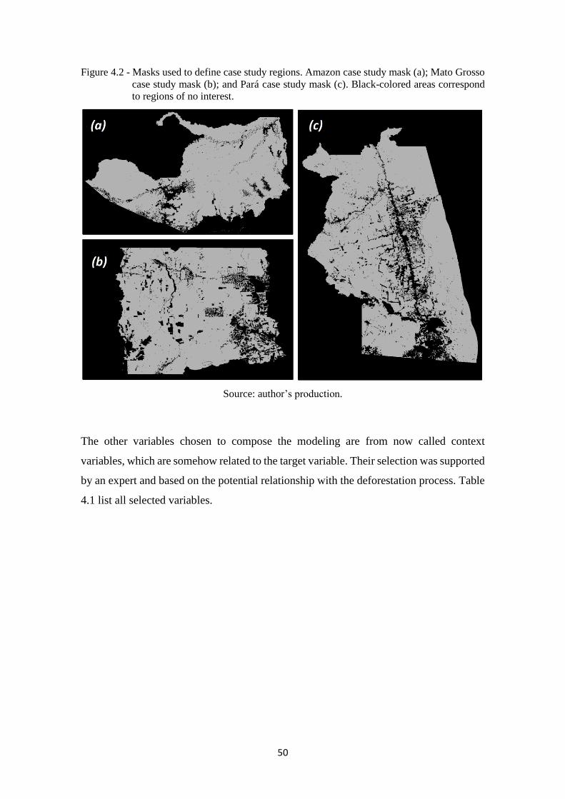
50
Figure 4.2 - Masks used to define case study regions. Amazon case study mask (a); Mato Grosso
case study mask (b); and Pará case study mask (c). Black-colored areas correspond
to regions of no interest.
Source: author’s production.
The other variables chosen to compose the modeling are from now called context
variables, which are somehow related to the target variable. Their selection was supported
by an expert and based on the potential relationship with the deforestation process. Table
4.1 list all selected variables.
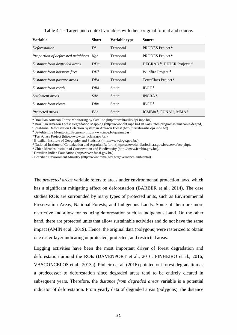
51
Table 4.1 - Target and context variables with their original format and source.
Variable Short Variable type Source
Deforestation Df Temporal PRODES Project a
Proportion of deforested neighbors Ngb Temporal PRODES Project a
Distance from degraded areas DDa Temporal DEGRAD b, DETER Projects c
Distance from hotspots fires DHf Temporal Wildfire Project d
Distance from pasture areas DPa Temporal TerraClass Project e
Distance from roads DRd Static IBGE f
Settlement areas SAr Static INCRA g
Distance from rivers DRv Static IBGE f
Protected areas PAr Static ICMBio h, FUNAI i, MMA j
a Brazilian Amazon Forest Monitoring by Satellite (http://terrabrasilis.dpi.inpe.br/). b Brazilian Amazon Forest Degradation Mapping (http://www.obt.inpe.br/OBT/assuntos/programas/amazonia/degrad). c Real-time Deforestation Detection System in Amazon Forest (http://terrabrasilis.dpi.inpe.br/). d Sattelite Fire Monitoring Program (http://www.inpe.br/queimadas) e TerraClass Project (https://www.terraclass.gov.br/) f Brazilian Institute of Geography and Statistics (http://www.ibge.gov.br/). g National Institute of Colonization and Agrarian Reform (http://acervofundiario.incra.gov.br/acervo/acv.php). h Chico Mendes Institute of Conservation and Biodiversity (http://www.icmbio.gov.br/). i Brazilian Indian Foundation (http://www.funai.gov.br/). j Brazilian Environment Ministry (http://www.mma.gov.br/governanca-ambiental).
The protected areas variable refers to areas under environmental protection laws, which
has a significant mitigating effect on deforestation (BARBER et al., 2014). The case
studies ROIs are surrounded by many types of protected units, such as Environmental
Preservation Areas, National Forests, and Indigenous Lands. Some of them are more
restrictive and allow for reducing deforestation such as Indigenous Land. On the other
hand, there are protected units that allow sustainable activities and do not have the same
impact (AMIN et al., 2019). Hence, the original data (polygons) were rasterized to obtain
one raster layer indicating unprotected, protected, and restricted areas.
Logging activities have been the most important driver of forest degradation and
deforestation around the ROIs (DAVENPORT et al., 2016; PINHEIRO et al., 2016;
VASCONCELOS et al., 2013a). Pinheiro et al. (2016) pointed out forest degradation as
a predecessor to deforestation since degraded areas tend to be entirely cleared in
subsequent years. Therefore, the distance from degraded areas variable is a potential
indicator of deforestation. From yearly data of degraded areas (polygons), the distance
52
(in meters) to the nearest edge of degraded area for each pixel was calculated. The result
is a raster time series with raster layers referring to the distance to yearly degraded areas.
Besides turning closed forests into degraded areas, logging activities also turn forest
highly vulnerable to droughts and fires (VASCONCELOS et al., 2013a). Indeed, fires
occurrence is one of the leading causes of forest degradation and deforestation (SETZER
et al., 2012; TASKER; ARIMA, 2016). Thus, the distance from hotspots fires variable is
another potential indicator of deforestation. From the hotspots fires data (points) clustered
annually, the distance (in meters) to the nearest hotspot fire for each pixel was calculated.
The result is a raster time series, in which each layer refers to the distance to yearly
hotspots fires.
Cattle-ranching expansion is also a significant driver of deforestation (BARONA et al.,
2010; SOLER; VERBURG; ALVES, 2014). As presented by Almeida et al. (2016)
pasture areas occupy most of the deforested areas in the BLA, as in the case study ROIs.
Thus, the distance from pasture areas was selected as an indicator of deforestation.
LULCC annual maps from the TerraClass project (ALMEIDA et al., 2016) were
processed to a raster time series with each layer representing yearly pasture and non-
pasture areas. For each raster layer, the distance to the nearest pasture area for each pixel
was calculated.
The construction of new roads allows access to previously inaccessible forests.
Subsequently, it leads to forest fragmentation, new colonizations, and increases fire risk,
as stated by Barber et al. (2014). The authors also verified more than 90% of all
deforestation in the BLA occurred within 5.5 𝑘𝑚 of roads. Consequently, the distance
from roads variable should be considered as a deforestation indicator. From the road
network data (lines) with the principal roads only, one raster layer was generated with the
distance (in meters) to the nearest road for each pixel.
Major roads stimulate deforestation by facilitating the construction of smaller side roads
as well as human settlements in remote areas (FEARNSIDE, 2015). Indeed, studies have
shown that settlements with human activities (e.g., agriculture and logging) play a major
role in deforestation (CHEN et al., 2015; TRITSCH; LE TOURNEAU, 2016) and fires
occurrences (ALENCAR et al., 2015). Therefore, the settlement area variable can be
considered as a deforestation indicator. The original data (polygons) were rasterized to
obtain one raster layer indicating undersigned and settlement areas.
53
Despite roads make way for previously inaccessible areas, several locations in the BLA
do not offer road accesses. The only access to roadless municipality and villages is via
navigable rivers (JUSYS, 2016). According to Barber et al. (2014), navigable rivers
provide another potential mode of access to untouchable forest regions and further
promote logging and deforestation. The authors also show that most deforested areas in
the BLA are located near to roads or navigable rivers. Consequently, the distance from
rivers variable also should be considered as a deforestation indicator. From the river
network data (lines), one raster layer was generated with the distance (in meters) to the
nearest river for each pixel.
Ongoing forest fragmentation increases the changes of forest destruction in general since
fragmented forests are far more susceptible to droughts, fires, logging, and any
anthropogenic impact (ALENCAR et al., 2015; LAURANCE et al., 2018). Forest
fragmentation creates forest areas susceptible to edge effects and, for accessibility
reasons, deforestation tends to occur near to already deforested areas (BROADBEND et
al., 2008). Therefore, the proportion of deforested neighbors variable was also selected
as a deforestation indicator. To compute this variable, the original data (polygons) were
processed to a raster time series with each layer containing the cumulative deforested and
forested areas. The proportion of deforested neighbors for each pixel was calculated from
a 5 x 5 moving window.
All the raster data collected and described above can be separated into two categories:
static and temporal variables. Static variables are those features that are assumed to stay
constant over time either because it is an inherent characteristic or due to the lack of
information to update them (ROSA et al., 2015). Among the selected variables, protected
areas, distance from roads, settlements areas, and distance from rivers are static
variables. By contrast, temporal variables are those features that change over time, which
were calculated for each time interval within the analysis period (ROSA et al., 2015).
Hence, deforestation, distance from degraded areas, distance from hotspots fires,
distance from pasture areas, and proportion of deforested neighbors are temporal
variables. Since the data pre-processing was carried out using R software, all variables
raster data are already as Raster* objects, i.e., RasterLayer for static variables or
RasterStack for temporal variables, as required by the stbnR package. Moreover, all raster
data are in the SIRGAS2000 coordinate reference system.
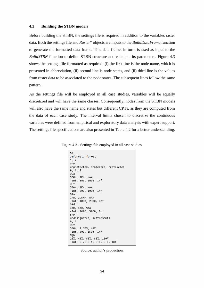
54
4.3 Building the STBN models
Before building the STBN, the settings file is required in addition to the variables raster
data. Both the settings file and Raster* objects are inputs to the BuildDataFrame function
to generate the formatted data frame. This data frame, in turn, is used as input to the
BuildSTBN function to define STBN structure and calculate its parameters. Figure 4.3
shows the settings file formatted as required: (i) the first line is the node name, which is
presented in abbreviation, (ii) second line is node states, and (ii) third line is the values
from raster data to be associated to the node states. The subsequent lines follow the same
pattern.
As the settings file will be employed in all case studies, variables will be equally
discretized and will have the same classes. Consequently, nodes from the STBN models
will also have the same name and states but different CPTs, as they are computed from
the data of each case study. The interval limits chosen to discretize the continuous
variables were defined from empirical and exploratory data analysis with expert support.
The settings file specifications are also presented in Table 4.2 for a better understanding.
Figure 4.3 - Settings file employed in all case studies.
Source: author’s production.
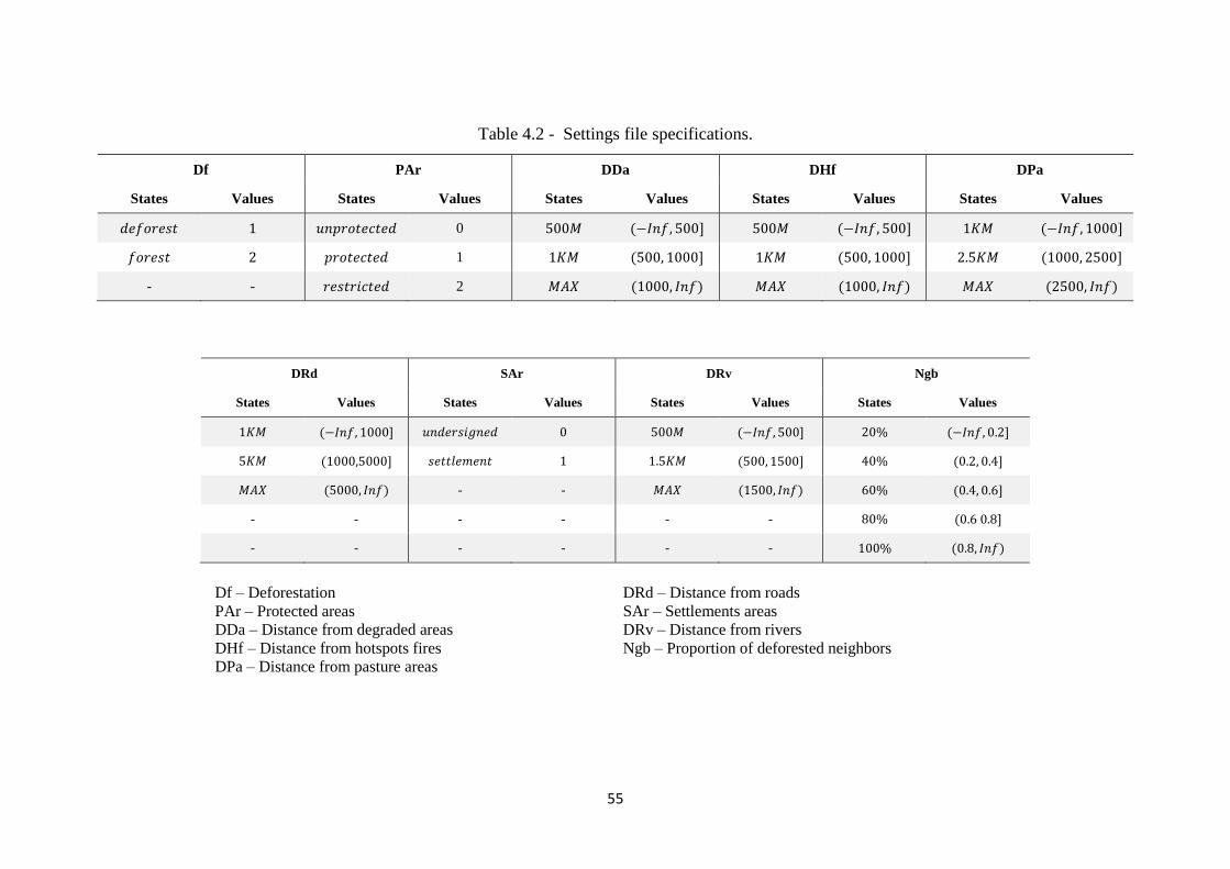
55
Table 4.2 - Settings file specifications.
Df PAr DDa DHf DPa
States Values States Values States Values States Values States Values
𝑑𝑒𝑓𝑜𝑟𝑒𝑠𝑡 1 𝑢𝑛𝑝𝑟𝑜𝑡𝑒𝑐𝑡𝑒𝑑 0 500𝑀 (−𝐼𝑛𝑓, 500] 500𝑀 (−𝐼𝑛𝑓, 500] 1𝐾𝑀 (−𝐼𝑛𝑓, 1000]
𝑓𝑜𝑟𝑒𝑠𝑡 2 𝑝𝑟𝑜𝑡𝑒𝑐𝑡𝑒𝑑 1 1𝐾𝑀 (500, 1000] 1𝐾𝑀 (500, 1000] 2.5𝐾𝑀 (1000, 2500]
- - 𝑟𝑒𝑠𝑡𝑟𝑖𝑐𝑡𝑒𝑑 2 𝑀𝐴𝑋 (1000, 𝐼𝑛𝑓) 𝑀𝐴𝑋 (1000, 𝐼𝑛𝑓) 𝑀𝐴𝑋 (2500, 𝐼𝑛𝑓)
DRd SAr DRv Ngb
States Values States Values States Values States Values
1𝐾𝑀 (−𝐼𝑛𝑓, 1000] 𝑢𝑛𝑑𝑒𝑟𝑠𝑖𝑔𝑛𝑒𝑑 0 500𝑀 (−𝐼𝑛𝑓, 500] 20% (−𝐼𝑛𝑓, 0.2]
5𝐾𝑀 (1000,5000] 𝑠𝑒𝑡𝑡𝑙𝑒𝑚𝑒𝑛𝑡 1 1.5𝐾𝑀 (500, 1500] 40% (0.2, 0.4]
𝑀𝐴𝑋 (5000, 𝐼𝑛𝑓) - - 𝑀𝐴𝑋 (1500, 𝐼𝑛𝑓) 60% (0.4, 0.6]
- - - - - - 80% (0.6 0.8]
- - - - - - 100% (0.8, 𝐼𝑛𝑓)
Df – Deforestation
PAr – Protected areas
DDa – Distance from degraded areas
DHf – Distance from hotspots fires
DPa – Distance from pasture areas
DRd – Distance from roads
SAr – Settlements areas
DRv – Distance from rivers
Ngb – Proportion of deforested neighbors
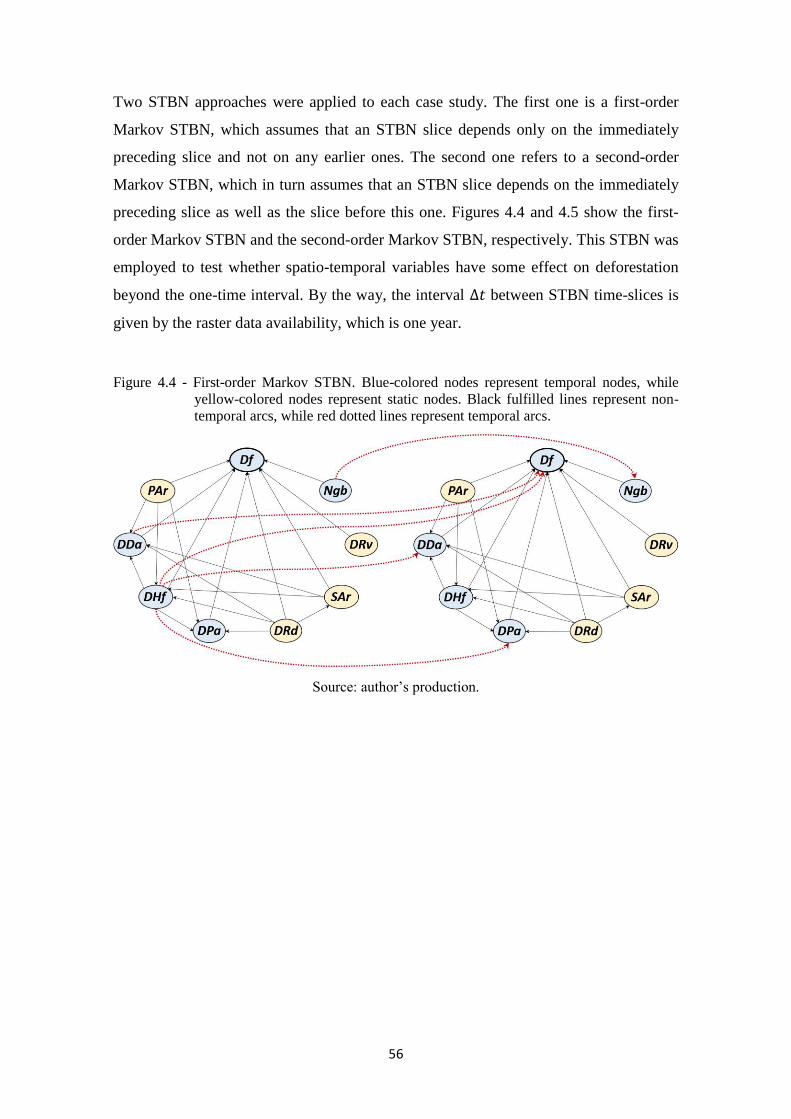
56
Two STBN approaches were applied to each case study. The first one is a first-order
Markov STBN, which assumes that an STBN slice depends only on the immediately
preceding slice and not on any earlier ones. The second one refers to a second-order
Markov STBN, which in turn assumes that an STBN slice depends on the immediately
preceding slice as well as the slice before this one. Figures 4.4 and 4.5 show the first-
order Markov STBN and the second-order Markov STBN, respectively. This STBN was
employed to test whether spatio-temporal variables have some effect on deforestation
beyond the one-time interval. By the way, the interval ∆𝑡 between STBN time-slices is
given by the raster data availability, which is one year.
Figure 4.4 - First-order Markov STBN. Blue-colored nodes represent temporal nodes, while
yellow-colored nodes represent static nodes. Black fulfilled lines represent non-
temporal arcs, while red dotted lines represent temporal arcs.
Source: author’s production.
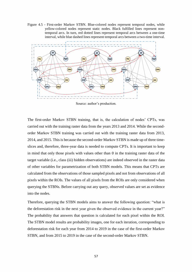
57
Figure 4.5 - First-order Markov STBN. Blue-colored nodes represent temporal nodes, while
yellow-colored nodes represent static nodes. Black fulfilled lines represent non-
temporal arcs. In turn, red dotted lines represent temporal arcs between a one-time
interval, while blue dashed lines represent temporal arcs between a two-time interval.
Source: author’s production.
The first-order Markov STBN training, that is, the calculation of nodes’ CPTs, was
carried out with the training raster data from the years 2013 and 2014. While the second-
order Markov STBN training was carried out with the training raster data from 2013,
2014, and 2015. This is because the second-order Markov STBN is made up of three time-
slices and, therefore, three-year data is needed to compute CPTs. It is important to keep
in mind that only those pixels with values other than 0 in the training raster data of the
target variable (i.e., class (iii) hidden observations) are indeed observed in the raster data
of other variables for parametrization of both STBN models. This means that CPTs are
calculated from the observations of those sampled pixels and not from observations of all
pixels within the ROIs. The values of all pixels from the ROIs are only considered when
querying the STBNs. Before carrying out any query, observed values are set as evidence
into the nodes.
Therefore, querying the STBN models aims to answer the following question: “what is
the deforestation risk in the next year given the observed evidence in the current year?”
The probability that answers that question is calculated for each pixel within the ROI.
The STBN model results are probability images, one for each iteration, corresponding to
deforestation risk for each year from 2014 to 2019 in the case of the first-order Markov
STBN, and from 2015 to 2019 in the case of the second-order Markov STBN.
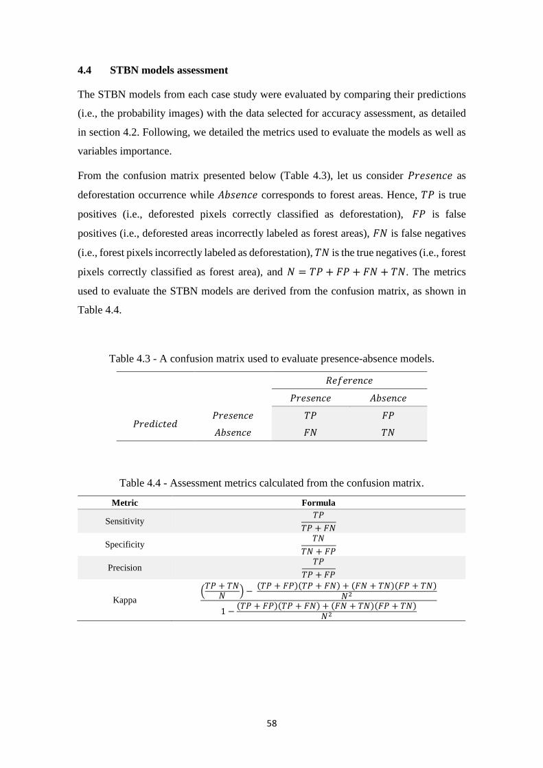
58
4.4 STBN models assessment
The STBN models from each case study were evaluated by comparing their predictions
(i.e., the probability images) with the data selected for accuracy assessment, as detailed
in section 4.2. Following, we detailed the metrics used to evaluate the models as well as
variables importance.
From the confusion matrix presented below (Table 4.3), let us consider 𝑃𝑟𝑒𝑠𝑒𝑛𝑐𝑒 as
deforestation occurrence while 𝐴𝑏𝑠𝑒𝑛𝑐𝑒 corresponds to forest areas. Hence, 𝑇𝑃 is true
positives (i.e., deforested pixels correctly classified as deforestation), 𝐹𝑃 is false
positives (i.e., deforested areas incorrectly labeled as forest areas), 𝐹𝑁 is false negatives
(i.e., forest pixels incorrectly labeled as deforestation), 𝑇𝑁 is the true negatives (i.e., forest
pixels correctly classified as forest area), and 𝑁 = 𝑇𝑃 + 𝐹𝑃 + 𝐹𝑁 + 𝑇𝑁. The metrics
used to evaluate the STBN models are derived from the confusion matrix, as shown in
Table 4.4.
Table 4.3 - A confusion matrix used to evaluate presence-absence models.
𝑅𝑒𝑓𝑒𝑟𝑒𝑛𝑐𝑒
𝑃𝑟𝑒𝑠𝑒𝑛𝑐𝑒 𝐴𝑏𝑠𝑒𝑛𝑐𝑒
𝑃𝑟𝑒𝑑𝑖𝑐𝑡𝑒𝑑 𝑃𝑟𝑒𝑠𝑒𝑛𝑐𝑒 𝑇𝑃 𝐹𝑃
𝐴𝑏𝑠𝑒𝑛𝑐𝑒 𝐹𝑁 𝑇𝑁
Table 4.4 - Assessment metrics calculated from the confusion matrix.
Metric Formula
Sensitivity 𝑇𝑃
𝑇𝑃 + 𝐹𝑁
Specificity 𝑇𝑁
𝑇𝑁 + 𝐹𝑃
Precision 𝑇𝑃
𝑇𝑃 + 𝐹𝑃
Kappa (
𝑇𝑃 + 𝑇𝑁𝑁
) − (𝑇𝑃 + 𝐹𝑃)(𝑇𝑃 + 𝐹𝑁) + (𝐹𝑁 + 𝑇𝑁)(𝐹𝑃 + 𝑇𝑁)
𝑁2
1 −(𝑇𝑃 + 𝐹𝑃)(𝑇𝑃 + 𝐹𝑁) + (𝐹𝑁 + 𝑇𝑁)(𝐹𝑃 + 𝑇𝑁)
𝑁2
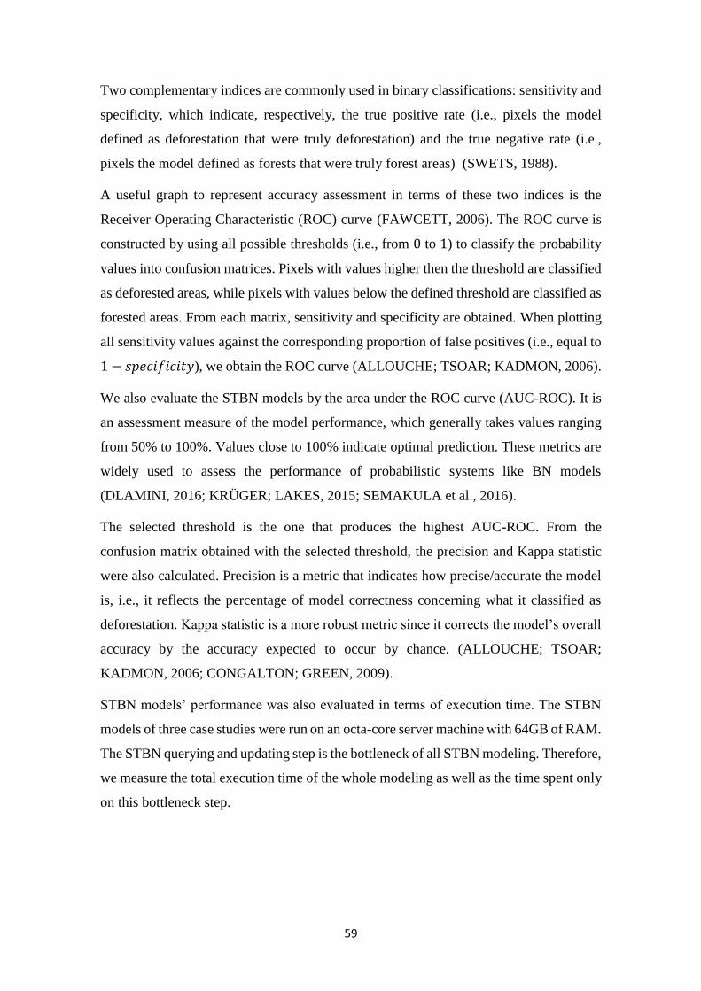
59
Two complementary indices are commonly used in binary classifications: sensitivity and
specificity, which indicate, respectively, the true positive rate (i.e., pixels the model
defined as deforestation that were truly deforestation) and the true negative rate (i.e.,
pixels the model defined as forests that were truly forest areas) (SWETS, 1988).
A useful graph to represent accuracy assessment in terms of these two indices is the
Receiver Operating Characteristic (ROC) curve (FAWCETT, 2006). The ROC curve is
constructed by using all possible thresholds (i.e., from 0 to 1) to classify the probability
values into confusion matrices. Pixels with values higher then the threshold are classified
as deforested areas, while pixels with values below the defined threshold are classified as
forested areas. From each matrix, sensitivity and specificity are obtained. When plotting
all sensitivity values against the corresponding proportion of false positives (i.e., equal to
1 − 𝑠𝑝𝑒𝑐𝑖𝑓𝑖𝑐𝑖𝑡𝑦), we obtain the ROC curve (ALLOUCHE; TSOAR; KADMON, 2006).
We also evaluate the STBN models by the area under the ROC curve (AUC-ROC). It is
an assessment measure of the model performance, which generally takes values ranging
from 50% to 100%. Values close to 100% indicate optimal prediction. These metrics are
widely used to assess the performance of probabilistic systems like BN models
(DLAMINI, 2016; KRÜGER; LAKES, 2015; SEMAKULA et al., 2016).
The selected threshold is the one that produces the highest AUC-ROC. From the
confusion matrix obtained with the selected threshold, the precision and Kappa statistic
were also calculated. Precision is a metric that indicates how precise/accurate the model
is, i.e., it reflects the percentage of model correctness concerning what it classified as
deforestation. Kappa statistic is a more robust metric since it corrects the model’s overall
accuracy by the accuracy expected to occur by chance. (ALLOUCHE; TSOAR;
KADMON, 2006; CONGALTON; GREEN, 2009).
STBN models’ performance was also evaluated in terms of execution time. The STBN
models of three case studies were run on an octa-core server machine with 64GB of RAM.
The STBN querying and updating step is the bottleneck of all STBN modeling. Therefore,
we measure the total execution time of the whole modeling as well as the time spent only
on this bottleneck step.
60
To quantify the influence of the predictor variables on the target variable, we used Mutual
Information (MI), which is defined within the information theory. MI measures how
much knowing one variable reduces the uncertainty about the other. In other words, it is
a measure of the amount of information that one random variable has about another
variable. In this sense, MI is zero when both variables are statistically independent
(VERGARA; ESTÉVEZ, 2014). The MI of two variables 𝑋 and 𝑌 is given by the
following equation:
Here, 𝑃(𝑋 = 𝑥) and 𝑃(𝑌 = 𝑌) are marginal probabilities and 𝑃(𝑋 = 𝑥, 𝑌 = 𝑌) is the
joint probability distribution.
𝑀𝐼(𝑋, 𝑌) = ∑ ∑ 𝑃(𝑋 = 𝑥, 𝑌 = 𝑦) ∗ log𝑃(𝑋 = 𝑥, 𝑌 = 𝑦)
𝑃(𝑋 = 𝑥)𝑃(𝑌 = 𝑦)
𝑛
𝑦
𝑛
𝑥
(4.1)
61
5 RESULTS AND DISCUSSION
This chapter presents the deforestation risk predictions obtained with STBN models. The
analyses and evaluation of results are presented by case studies. First, the Amazon case
study is presented, followed by Mato Grosso case study, and last the Para case study.
Two STBNs approaches were applied in each case study. The first-order Markov STBN
was trained with raster data from 2013 and 2014. Thus, predictions were made for the
year 2014 onwards. As raster data were observed until 2018, the last prediction was made
for 2019, so the result of the first-order Markov STBN is a six-layer raster time series,
one for each year from 2014 to 2019. On the other hand, the second-order Markov STBN
was trained with raster data from 2013, 2014, and 2015, as it is made up of three time-
slices. Thus, predictions were made for the year 2015 until 2019, and, therefore, the result
of this STNB approach is a five-layer raster time series.
Each raster layer (from both STBN models) corresponds to a probability image, in which
every pixel value within the ROI represents the probability that location be deforested
given observation on the context variables. From the visual analysis, it is not possible to
notice significant differences among the probability images resulting from both STBN
models. Regions with the highest deforestation risk are indicated by red-colored pixels in
the Figures, while dark green-colored pixels indicate the contrary. White pixels within
the ROIs refer to previously deforested areas (i.e., before the prediction year). These areas
were removed from the probability images since there is no interest in prediction
assessment in areas already deforested.
The probability images with deforestation risk over the year can be considered the main
result of the STBN models developed from the stbnR package. The analyzes carried out
from now onwards no longer concern the package implemented in this thesis. Thus, we
evaluated the probability image time series in each case study by comparing them with
those datasets previously selected to perform model accuracy assessment. We analyze the
distribution of the probability values for the target presence and absence classes (i.e.,
deforested and forested areas, respectively). In general, predictions were consistent, so
that the highest probability values were assigned to the majority of deforested pixels,
while the lowest probability values were assigned to the majority of forest pixels.
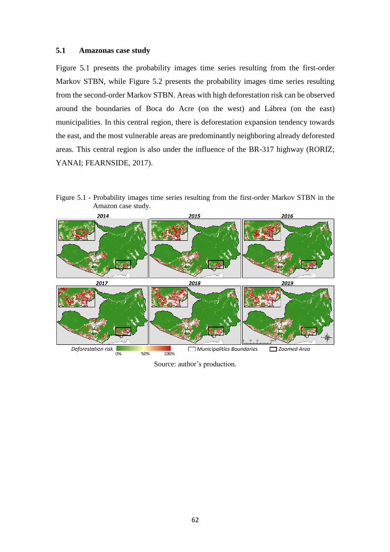
62
5.1 Amazonas case study
Figure 5.1 presents the probability images time series resulting from the first-order
Markov STBN, while Figure 5.2 presents the probability images time series resulting
from the second-order Markov STBN. Areas with high deforestation risk can be observed
around the boundaries of Boca do Acre (on the west) and Lábrea (on the east)
municipalities. In this central region, there is deforestation expansion tendency towards
the east, and the most vulnerable areas are predominantly neighboring already deforested
areas. This central region is also under the influence of the BR-317 highway (RORIZ;
YANAI; FEARNSIDE, 2017).
Figure 5.1 - Probability images time series resulting from the first-order Markov STBN in the
Amazon case study.
Source: author’s production.
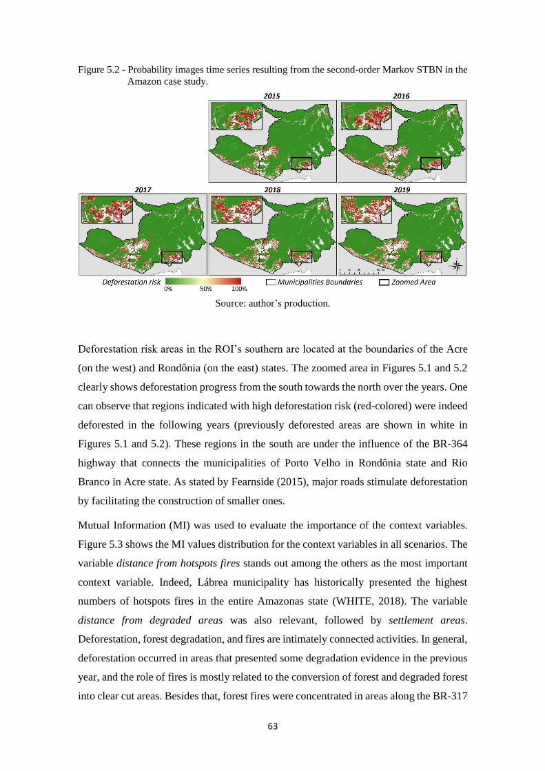
63
Figure 5.2 - Probability images time series resulting from the second-order Markov STBN in the
Amazon case study.
Source: author’s production.
Deforestation risk areas in the ROI’s southern are located at the boundaries of the Acre
(on the west) and Rondônia (on the east) states. The zoomed area in Figures 5.1 and 5.2
clearly shows deforestation progress from the south towards the north over the years. One
can observe that regions indicated with high deforestation risk (red-colored) were indeed
deforested in the following years (previously deforested areas are shown in white in
Figures 5.1 and 5.2). These regions in the south are under the influence of the BR-364
highway that connects the municipalities of Porto Velho in Rondônia state and Rio
Branco in Acre state. As stated by Fearnside (2015), major roads stimulate deforestation
by facilitating the construction of smaller ones.
Mutual Information (MI) was used to evaluate the importance of the context variables.
Figure 5.3 shows the MI values distribution for the context variables in all scenarios. The
variable distance from hotspots fires stands out among the others as the most important
context variable. Indeed, Lábrea municipality has historically presented the highest
numbers of hotspots fires in the entire Amazonas state (WHITE, 2018). The variable
distance from degraded areas was also relevant, followed by settlement areas.
Deforestation, forest degradation, and fires are intimately connected activities. In general,
deforestation occurred in areas that presented some degradation evidence in the previous
year, and the role of fires is mostly related to the conversion of forest and degraded forest
into clear cut areas. Besides that, forest fires were concentrated in areas along the BR-317
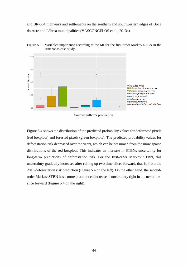
64
and BR-364 highways and settlements on the southern and southwestern edges of Boca
do Acre and Lábrea municipalities (VASCONCELOS et al., 2013a)
Figure 5.3 - Variables importance according to the MI for the first-order Markov STBN in the
Amazonas case study.
Source: author’s production.
Figure 5.4 shows the distribution of the predicted probability values for deforested pixels
(red boxplots) and forested pixels (green boxplots). The predicted probability values for
deforestation risk decreased over the years, which can be presumed from the more sparse
distributions of the red boxplots. This indicates an increase in STBNs uncertainty for
long-term predictions of deforestation risk. For the first-order Markov STBN, this
uncertainty gradually increases after rolling up two time-slices forward, that is, from the
2016 deforestation risk prediction (Figure 5.4 on the left). On the other hand, the second-
order Markov STBN has a more pronounced increase in uncertainty right in the next time-
slice forward (Figure 5.4 on the right).
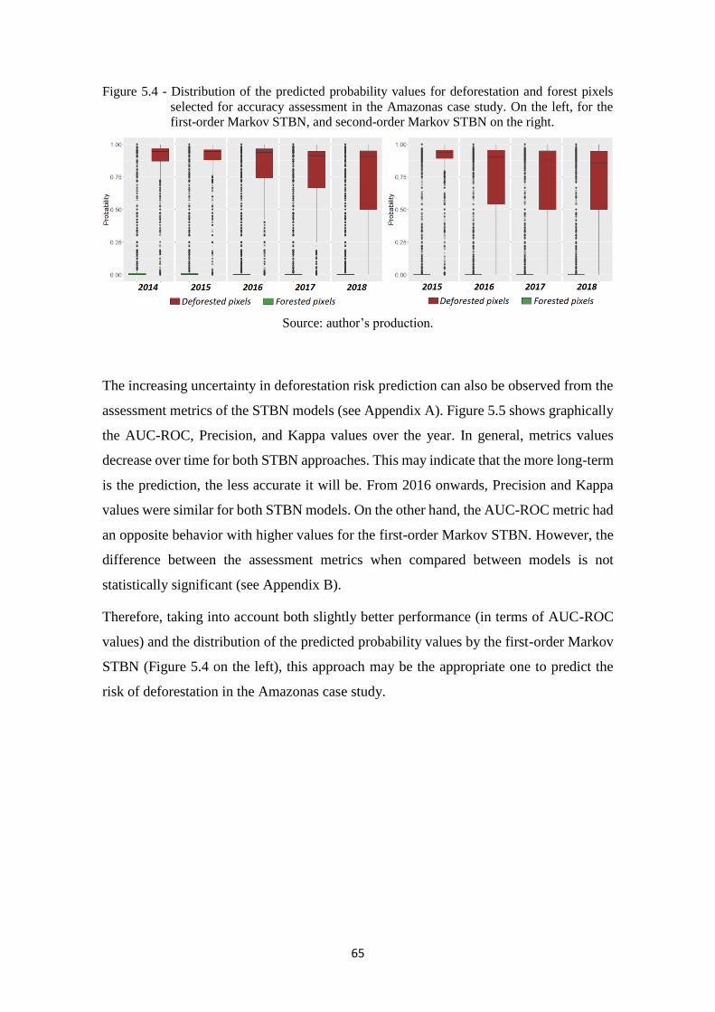
65
Figure 5.4 - Distribution of the predicted probability values for deforestation and forest pixels
selected for accuracy assessment in the Amazonas case study. On the left, for the
first-order Markov STBN, and second-order Markov STBN on the right.
Source: author’s production.
The increasing uncertainty in deforestation risk prediction can also be observed from the
assessment metrics of the STBN models (see Appendix A). Figure 5.5 shows graphically
the AUC-ROC, Precision, and Kappa values over the year. In general, metrics values
decrease over time for both STBN approaches. This may indicate that the more long-term
is the prediction, the less accurate it will be. From 2016 onwards, Precision and Kappa
values were similar for both STBN models. On the other hand, the AUC-ROC metric had
an opposite behavior with higher values for the first-order Markov STBN. However, the
difference between the assessment metrics when compared between models is not
statistically significant (see Appendix B).
Therefore, taking into account both slightly better performance (in terms of AUC-ROC
values) and the distribution of the predicted probability values by the first-order Markov
STBN (Figure 5.4 on the left), this approach may be the appropriate one to predict the
risk of deforestation in the Amazonas case study.
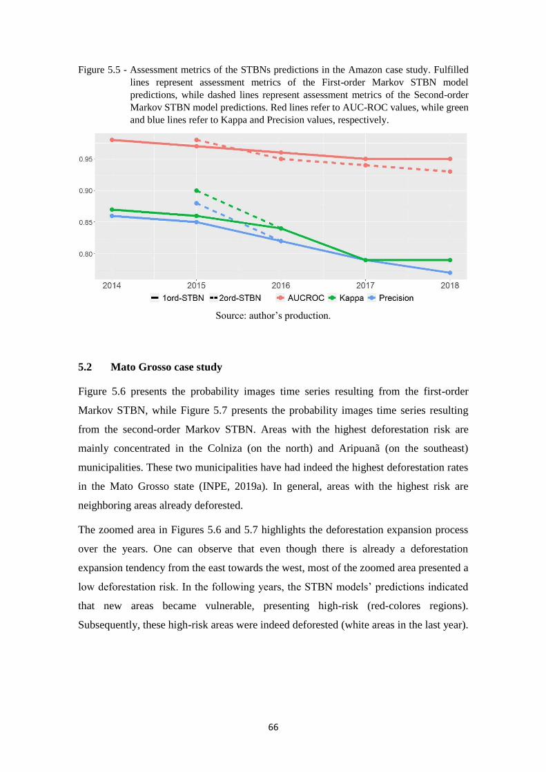
66
Figure 5.5 - Assessment metrics of the STBNs predictions in the Amazon case study. Fulfilled
lines represent assessment metrics of the First-order Markov STBN model
predictions, while dashed lines represent assessment metrics of the Second-order
Markov STBN model predictions. Red lines refer to AUC-ROC values, while green
and blue lines refer to Kappa and Precision values, respectively.
Source: author’s production.
5.2 Mato Grosso case study
Figure 5.6 presents the probability images time series resulting from the first-order
Markov STBN, while Figure 5.7 presents the probability images time series resulting
from the second-order Markov STBN. Areas with the highest deforestation risk are
mainly concentrated in the Colniza (on the north) and Aripuanã (on the southeast)
municipalities. These two municipalities have had indeed the highest deforestation rates
in the Mato Grosso state (INPE, 2019a). In general, areas with the highest risk are
neighboring areas already deforested.
The zoomed area in Figures 5.6 and 5.7 highlights the deforestation expansion process
over the years. One can observe that even though there is already a deforestation
expansion tendency from the east towards the west, most of the zoomed area presented a
low deforestation risk. In the following years, the STBN models’ predictions indicated
that new areas became vulnerable, presenting high-risk (red-colores regions).
Subsequently, these high-risk areas were indeed deforested (white areas in the last year).
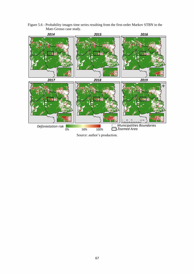
67
Figure 5.6 - Probability images time series resulting from the first-order Markov STBN in the
Mato Grosso case study.
Source: author’s production.
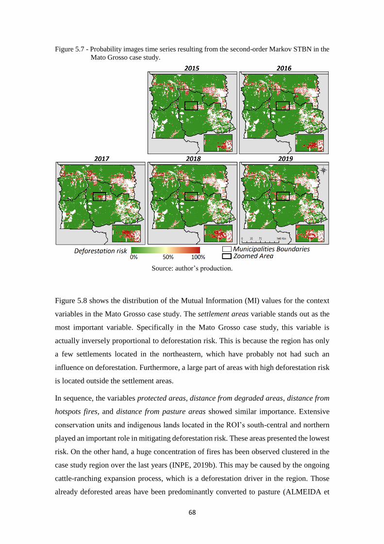
68
Figure 5.7 - Probability images time series resulting from the second-order Markov STBN in the
Mato Grosso case study.
Source: author’s production.
Figure 5.8 shows the distribution of the Mutual Information (MI) values for the context
variables in the Mato Grosso case study. The settlement areas variable stands out as the
most important variable. Specifically in the Mato Grosso case study, this variable is
actually inversely proportional to deforestation risk. This is because the region has only
a few settlements located in the northeastern, which have probably not had such an
influence on deforestation. Furthermore, a large part of areas with high deforestation risk
is located outside the settlement areas.
In sequence, the variables protected areas, distance from degraded areas, distance from
hotspots fires, and distance from pasture areas showed similar importance. Extensive
conservation units and indigenous lands located in the ROI’s south-central and northern
played an important role in mitigating deforestation risk. These areas presented the lowest
risk. On the other hand, a huge concentration of fires has been observed clustered in the
case study region over the last years (INPE, 2019b). This may be caused by the ongoing
cattle-ranching expansion process, which is a deforestation driver in the region. Those
already deforested areas have been predominantly converted to pasture (ALMEIDA et
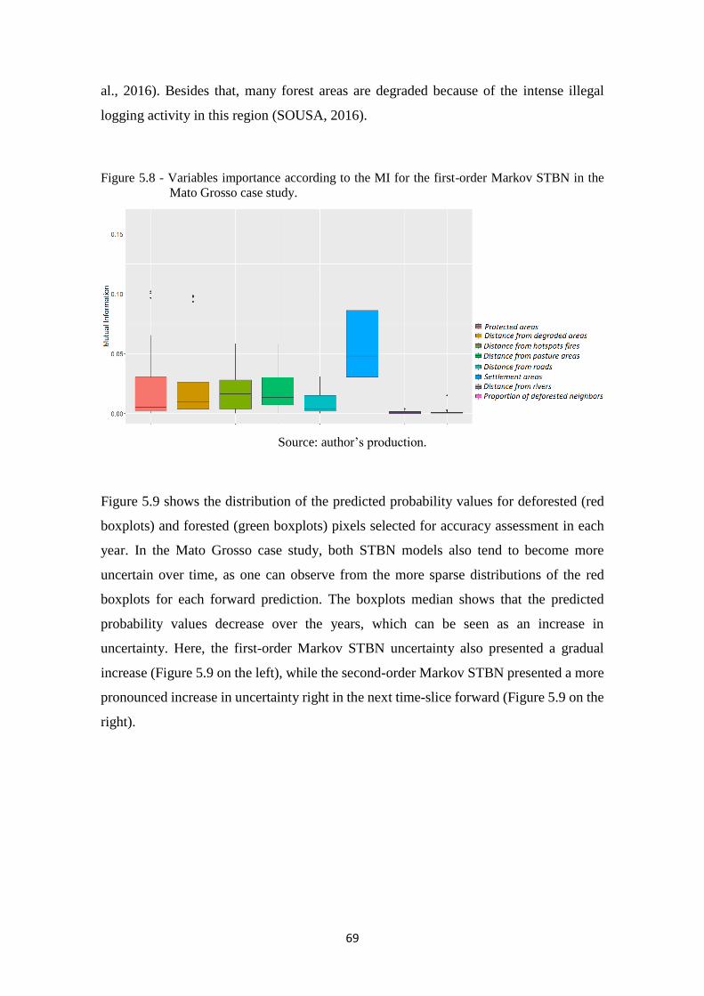
69
al., 2016). Besides that, many forest areas are degraded because of the intense illegal
logging activity in this region (SOUSA, 2016).
Figure 5.8 - Variables importance according to the MI for the first-order Markov STBN in the
Mato Grosso case study.
Source: author’s production.
Figure 5.9 shows the distribution of the predicted probability values for deforested (red
boxplots) and forested (green boxplots) pixels selected for accuracy assessment in each
year. In the Mato Grosso case study, both STBN models also tend to become more
uncertain over time, as one can observe from the more sparse distributions of the red
boxplots for each forward prediction. The boxplots median shows that the predicted
probability values decrease over the years, which can be seen as an increase in
uncertainty. Here, the first-order Markov STBN uncertainty also presented a gradual
increase (Figure 5.9 on the left), while the second-order Markov STBN presented a more
pronounced increase in uncertainty right in the next time-slice forward (Figure 5.9 on the
right).
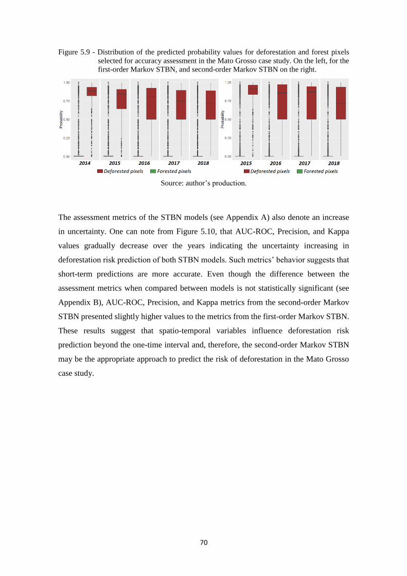
70
Figure 5.9 - Distribution of the predicted probability values for deforestation and forest pixels
selected for accuracy assessment in the Mato Grosso case study. On the left, for the
first-order Markov STBN, and second-order Markov STBN on the right.
Source: author’s production.
The assessment metrics of the STBN models (see Appendix A) also denote an increase
in uncertainty. One can note from Figure 5.10, that AUC-ROC, Precision, and Kappa
values gradually decrease over the years indicating the uncertainty increasing in
deforestation risk prediction of both STBN models. Such metrics’ behavior suggests that
short-term predictions are more accurate. Even though the difference between the
assessment metrics when compared between models is not statistically significant (see
Appendix B), AUC-ROC, Precision, and Kappa metrics from the second-order Markov
STBN presented slightly higher values to the metrics from the first-order Markov STBN.
These results suggest that spatio-temporal variables influence deforestation risk
prediction beyond the one-time interval and, therefore, the second-order Markov STBN
may be the appropriate approach to predict the risk of deforestation in the Mato Grosso
case study.
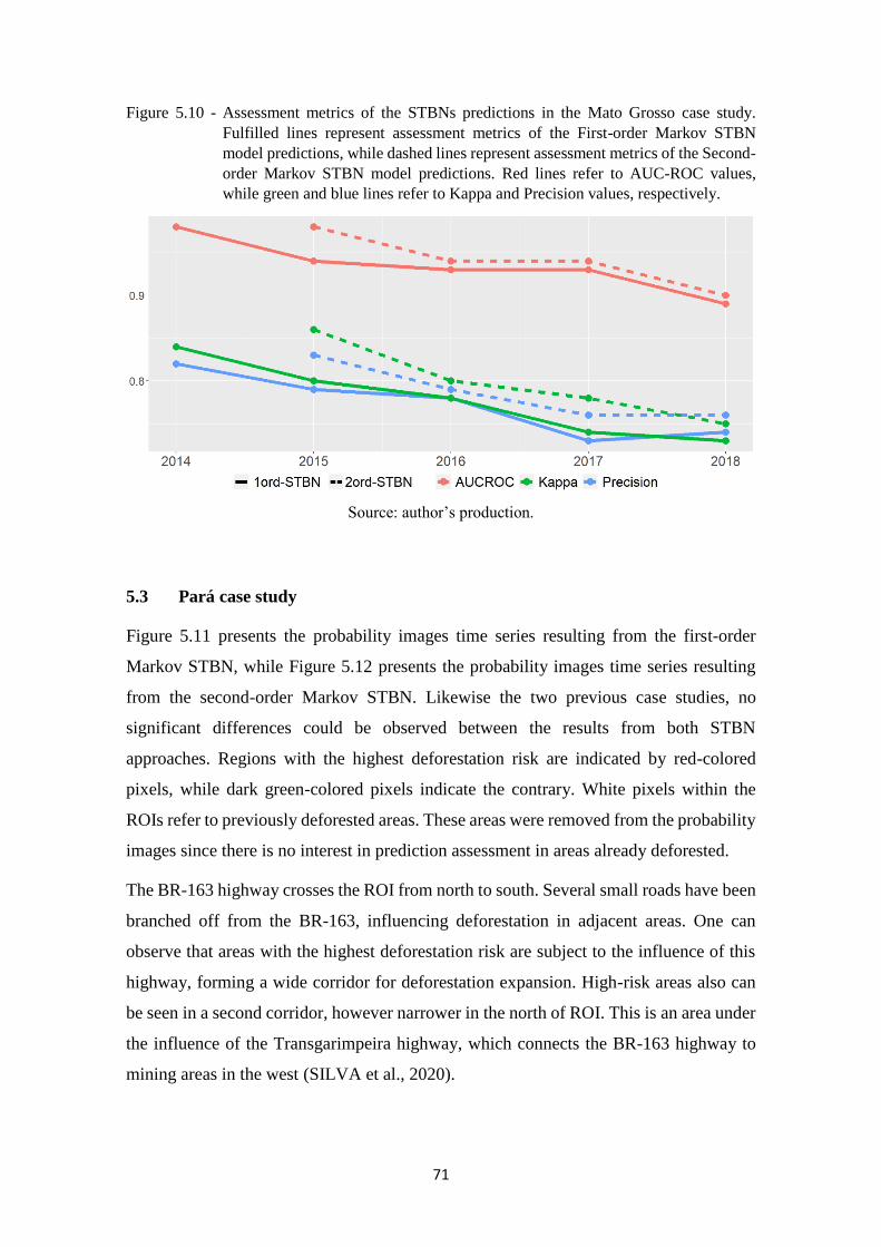
71
Figure 5.10 - Assessment metrics of the STBNs predictions in the Mato Grosso case study.
Fulfilled lines represent assessment metrics of the First-order Markov STBN
model predictions, while dashed lines represent assessment metrics of the Second-
order Markov STBN model predictions. Red lines refer to AUC-ROC values,
while green and blue lines refer to Kappa and Precision values, respectively.
Source: author’s production.
5.3 Pará case study
Figure 5.11 presents the probability images time series resulting from the first-order
Markov STBN, while Figure 5.12 presents the probability images time series resulting
from the second-order Markov STBN. Likewise the two previous case studies, no
significant differences could be observed between the results from both STBN
approaches. Regions with the highest deforestation risk are indicated by red-colored
pixels, while dark green-colored pixels indicate the contrary. White pixels within the
ROIs refer to previously deforested areas. These areas were removed from the probability
images since there is no interest in prediction assessment in areas already deforested.
The BR-163 highway crosses the ROI from north to south. Several small roads have been
branched off from the BR-163, influencing deforestation in adjacent areas. One can
observe that areas with the highest deforestation risk are subject to the influence of this
highway, forming a wide corridor for deforestation expansion. High-risk areas also can
be seen in a second corridor, however narrower in the north of ROI. This is an area under
the influence of the Transgarimpeira highway, which connects the BR-163 highway to
mining areas in the west (SILVA et al., 2020).
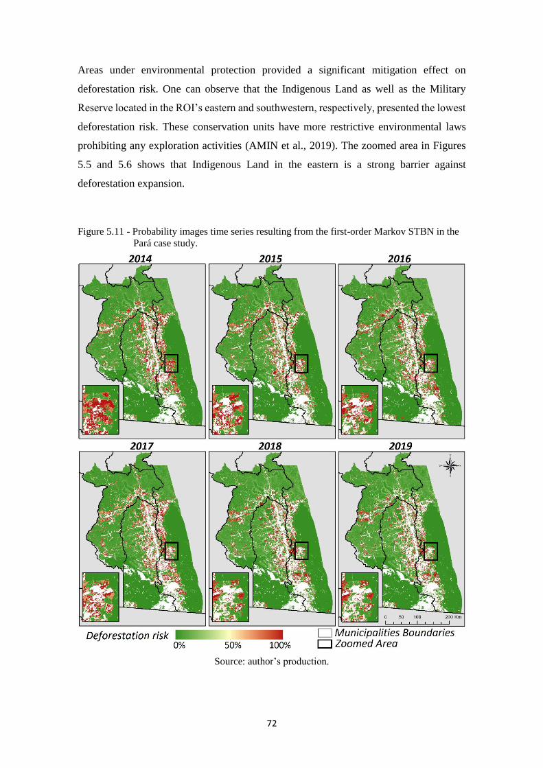
72
Areas under environmental protection provided a significant mitigation effect on
deforestation risk. One can observe that the Indigenous Land as well as the Military
Reserve located in the ROI’s eastern and southwestern, respectively, presented the lowest
deforestation risk. These conservation units have more restrictive environmental laws
prohibiting any exploration activities (AMIN et al., 2019). The zoomed area in Figures
5.5 and 5.6 shows that Indigenous Land in the eastern is a strong barrier against
deforestation expansion.
Figure 5.11 - Probability images time series resulting from the first-order Markov STBN in the
Pará case study.
Source: author’s production.
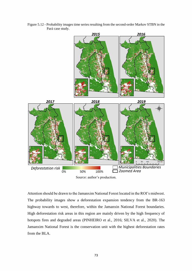
73
Figure 5.12 - Probability images time series resulting from the second-order Markov STBN in the
Pará case study.
Source: author’s production.
Attention should be drawn to the Jamanxim National Forest located in the ROI’s midwest.
The probability images show a deforestation expansion tendency from the BR-163
highway towards to west, therefore, within the Jamanxin National Forest boundaries.
High deforestation risk areas in this region are mainly driven by the high frequency of
hotspots fires and degraded areas (PINHEIRO et al., 2016; SILVA et al., 2020). The
Jamanxim National Forest is the conservation unit with the highest deforestation rates
from the BLA.
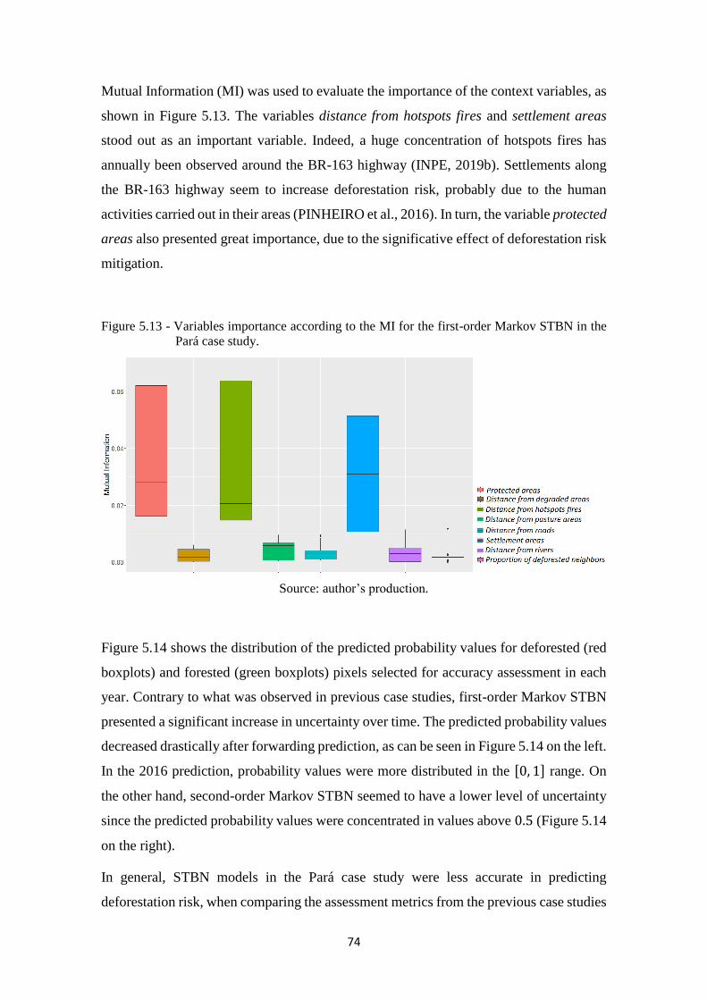
74
Mutual Information (MI) was used to evaluate the importance of the context variables, as
shown in Figure 5.13. The variables distance from hotspots fires and settlement areas
stood out as an important variable. Indeed, a huge concentration of hotspots fires has
annually been observed around the BR-163 highway (INPE, 2019b). Settlements along
the BR-163 highway seem to increase deforestation risk, probably due to the human
activities carried out in their areas (PINHEIRO et al., 2016). In turn, the variable protected
areas also presented great importance, due to the significative effect of deforestation risk
mitigation.
Figure 5.13 - Variables importance according to the MI for the first-order Markov STBN in the
Pará case study.
Source: author’s production.
Figure 5.14 shows the distribution of the predicted probability values for deforested (red
boxplots) and forested (green boxplots) pixels selected for accuracy assessment in each
year. Contrary to what was observed in previous case studies, first-order Markov STBN
presented a significant increase in uncertainty over time. The predicted probability values
decreased drastically after forwarding prediction, as can be seen in Figure 5.14 on the left.
In the 2016 prediction, probability values were more distributed in the [0, 1] range. On
the other hand, second-order Markov STBN seemed to have a lower level of uncertainty
since the predicted probability values were concentrated in values above 0.5 (Figure 5.14
on the right).
In general, STBN models in the Pará case study were less accurate in predicting
deforestation risk, when comparing the assessment metrics from the previous case studies
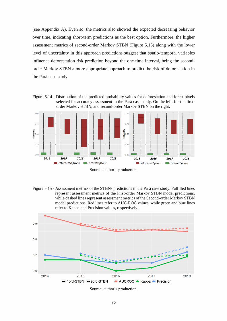
75
(see Appendix A). Even so, the metrics also showed the expected decreasing behavior
over time, indicating short-term predictions as the best option. Furthermore, the higher
assessment metrics of second-order Markov STBN (Figure 5.15) along with the lower
level of uncertainty in this approach predictions suggest that spatio-temporal variables
influence deforestation risk prediction beyond the one-time interval, being the second-
order Markov STBN a more appropriate approach to predict the risk of deforestation in
the Pará case study.
Figure 5.14 - Distribution of the predicted probability values for deforestation and forest pixels
selected for accuracy assessment in the Pará case study. On the left, for the first-
order Markov STBN, and second-order Markov STBN on the right.
Source: author’s production.
Figure 5.15 - Assessment metrics of the STBNs predictions in the Pará case study. Fulfilled lines
represent assessment metrics of the First-order Markov STBN model predictions,
while dashed lines represent assessment metrics of the Second-order Markov STBN
model predictions. Red lines refer to AUC-ROC values, while green and blue lines
refer to Kappa and Precision values, respectively.
Source: author’s production.
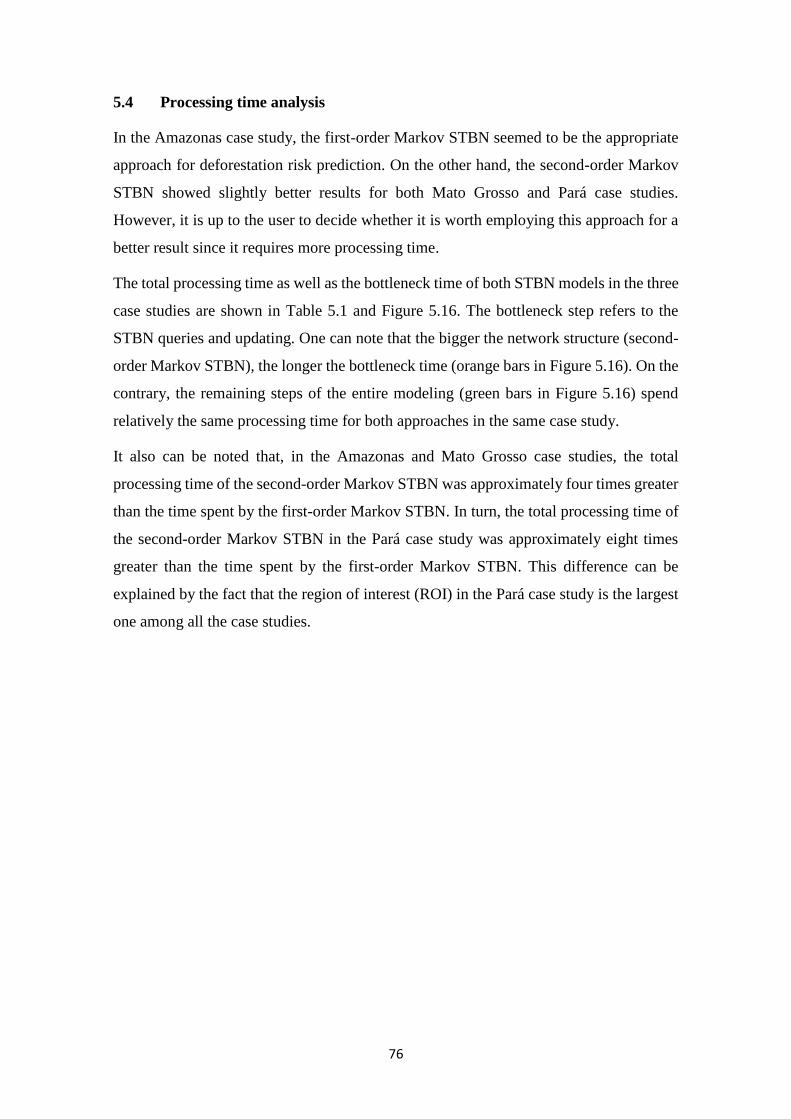
76
5.4 Processing time analysis
In the Amazonas case study, the first-order Markov STBN seemed to be the appropriate
approach for deforestation risk prediction. On the other hand, the second-order Markov
STBN showed slightly better results for both Mato Grosso and Pará case studies.
However, it is up to the user to decide whether it is worth employing this approach for a
better result since it requires more processing time.
The total processing time as well as the bottleneck time of both STBN models in the three
case studies are shown in Table 5.1 and Figure 5.16. The bottleneck step refers to the
STBN queries and updating. One can note that the bigger the network structure (second-
order Markov STBN), the longer the bottleneck time (orange bars in Figure 5.16). On the
contrary, the remaining steps of the entire modeling (green bars in Figure 5.16) spend
relatively the same processing time for both approaches in the same case study.
It also can be noted that, in the Amazonas and Mato Grosso case studies, the total
processing time of the second-order Markov STBN was approximately four times greater
than the time spent by the first-order Markov STBN. In turn, the total processing time of
the second-order Markov STBN in the Pará case study was approximately eight times
greater than the time spent by the first-order Markov STBN. This difference can be
explained by the fact that the region of interest (ROI) in the Pará case study is the largest
one among all the case studies.
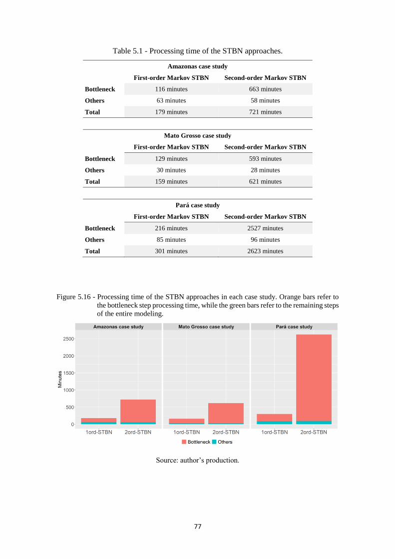
77
Table 5.1 - Processing time of the STBN approaches.
Amazonas case study
First-order Markov STBN Second-order Markov STBN
Bottleneck 116 minutes 663 minutes
Others 63 minutes 58 minutes
Total 179 minutes 721 minutes
Mato Grosso case study
First-order Markov STBN Second-order Markov STBN
Bottleneck 129 minutes 593 minutes
Others 30 minutes 28 minutes
Total 159 minutes 621 minutes
Pará case study
First-order Markov STBN Second-order Markov STBN
Bottleneck 216 minutes 2527 minutes
Others 85 minutes 96 minutes
Total 301 minutes 2623 minutes
Figure 5.16 - Processing time of the STBN approaches in each case study. Orange bars refer to
the bottleneck step processing time, while the green bars refer to the remaining steps
of the entire modeling.
Source: author’s production.
78
6 CONCLUSION
The main goal of this doctoral thesis was to build a Spatio-Temporal Bayesian Network
(STBN) model to predict deforestation risk. To accomplish the objective of this work, we
implemented an R package called stbnR (Spatio-Temporal Bayesian Network for R),
which allows the development of STBN-based LULCC models within a single integrated
environment, thus avoiding challenges such as data conversion and transfer from different
software tools. The stbnR package was developed in R because this is an open-source
programing language, which allows the proposed package to be thoroughly tested in
several applications. The stbnR package documentation is being finalized and will soon
be available on the GitHub website https://github.com/alexsandrocandido/stbnR and
maybe in the CRAN repository (Comprehensive R Archive Network).
We presented in the main functions of the stbnR package and how to use them to carry
out a complete workflow of LULCC modeling based on an STBN. Although employing
BNs to predict deforestation risk has been proposed before (DLAMINI, 2016; KRÜGER;
LAKES, 2015; MAYFIELD et al., 2017), the temporal domain has not been taken into
account, and deforestation has been considered as a static process when modeled by BN
approaches. Therefore, the STBN models developed in this work aimed to meet such
demand, by incorporating both spatial and temporal information into the modeling.
Three deforestation frontier regions in the Amazon Forest were selected to apply the
STBN models to evaluate them and demonstrate their potential in predicting deforestation
risk over time. For each case study region, two STBN approaches were applied: a first-
order Markov STBN and a second-order Markov STBN. Through the application of both
models, we were able to confirm the work’s hypothesis that STBN-based LULCC models
are able to capture and represent the variables’ spatio-temporal relationships to
appropriately predict deforestation risk.
The probability images time series are the main STBN models outputs. In each probability
image, each pixel value represents the probability of that location being deforested given
the values observed in the context variables. According to the accuracy assessment
indexes, the STBN models presented a strong performance with a great agreement
between deforestation events and predictions. Furthermore, the second-order Markov
STBN overperformed the first-order Markov STBN in two case study regions. This
79
indicates that deforestation risk prediction is influenced not only by variables in the
previous time-slice but also by variables from earlier time-slices.
However, we could note that there was an increase in uncertainty for both STBN models
in deforestation risk prediction over time, indicating that the more long-term is the
prediction, the less accurate it will be. Thus, we can state that STNB-based LULCC
models are suitable for short-term predictions. Besides the uncertainty increasing, the
second-order Markov STBN application can bring another concern about the execution
time. In the three case study regions, this model spent much more time than the first-order
Markov STBN. Therefore, even though computer systems currently offer sufficient
resources to perform robust tasks, the user may consider weighting between a better result
or a faster result.
Among the variables selected to compose the STBN models, the distance from hotspots
fires stood out as one of the most important variables for predicting deforestation risk.
This variable is directly related to human activities such as illegal logging and cattle-
ranching expansion, which are the main deforestation drivers in the Amazon forest. In
addition to that, the protected areas variable was also extremely important but not as a
driver but as a mitigator of deforestation risk. Indeed, the lowest values of risk were found
in conservation units such as indigenous land.
The probability images obtained from the STBN models can be used as indicators of the
areas most vulnerable to deforestation and support for decision-makers to implement
directed preventive action plans, for instance, focused on priority areas. As future work,
we suggest testing the application of STBN models with higher-order Markov for
predicting deforestation risk. These models may obtain more accurate results.
Furthermore, a thorough sensitivity analysis should be conducted to measure the impact
in the STBN models’ predictions from changes in the discretization thresholds of the
context variables as well as in the variables’ relationship. It is also important to test the
robustness of the stbnR package with available benchmarking to ensure its quality. In
addition to that, we also suggest the development of STBN-based LULCC models from
the stbnR package for other Earth observation applications besides the deforestation
process.

80
REFERENCES
ABEBE, Y.; KABIR, G.; TESFAMARIAM, S. Assessing urban areas vulnerability to
pluvial flooding using GIS applications and Bayesian Belief Network model. Journal
of Cleaner Production, v. 174, p. 1629–1641, Feb. 2018.
ABIDEN, M. Z. Z. et al. Comparative study on stochastic and deterministic
approaches in urban growth model. In: IEEE INTERNATIONAL COLLOQUIUM
ON SIGNAL PROCESSING AND ITS APPLICATIONS, 9., 2013. Anais...IEEE,
2013. Available from: <http://ieeexplore.ieee.org/document/6530064/>.
ABURAS, M. M.; AHAMAD, M. S. S.; OMAR, N. Q. Spatio-temporal simulation and
prediction of land-use change using conventional and machine learning models: a
review. Environmental Monitoring and Assessment, v. 191, n. 4, p. 205, 5 Apr. 2019.
AGUILERA, P. A. et al. Bayesian networks in environmental modelling.
Environmental Modelling & Software, v. 26, n. 12, p. 1376–1388, Dec. 2011.
AITKENHEAD, M. J.; AALDERS, I. H. Predicting land cover using GIS, Bayesian and
evolutionary algorithm methods. Journal of Environmental Management, v. 90, n. 1,
p. 236–250, 2009.
AL-SHARIF, A. A. A.; PRADHAN, B. Spatio-temporal prediction of urban expansion
using bivariate statistical models: assessment of the efficacy of evidential belief
functions and frequency ratio models. Applied Spatial Analysis and Policy, v. 9, n. 2,
p. 213–231, 8 June. 2016.
ALENCAR, A. A. et al. Landscape fragmentation, severe drought, and the new Amazon
forest fire regime. Ecological Applications, v. 25, n. 6, p. 1493–1505, Sept. 2015.
ALLOUCHE, O.; TSOAR, A.; KADMON, R. Assessing the accuracy of species
distribution models: prevalence, kappa and the True Skill Statistic (TSS). Journal of
Applied Ecology, v. 43, n. 6, p. 1223–1232, 12 Sept. 2006.
ALMEIDA, C. A. DE et al. High spatial resolution land use and land cover mapping of
the Brazilian Legal Amazon in 2008 using Landsat-5/TM and MODIS data. Acta
Amazonica, v. 46, n. 3, p. 291–302, Sept. 2016.
81
ALVES, L. M. et al. Sensitivity of Amazon regional climate to deforestation. American
Journal of Climate Change, v. 06, n. 01, p. 75–98, 2017.
AMIN, A. et al. Neighborhood effects in the Brazilian Amazônia: protected areas and
deforestation. Journal of Environmental Economics and Management, v. 93, p.
272–288, Jan. 2019.
ARIMA, E. Y. et al. Public policies can reduce tropical deforestation: lessons and
challenges from Brazil. Land Use Policy, v. 41, p. 465–473, Nov. 2014.
ARTAXO, P. Working together for Amazonia. Science, v. 363, n. 6425, p. 323–323, 25
Jan. 2019.
BALBI, S. et al. A spatial Bayesian network model to assess the benefits of early
warning for urban flood risk to people. Natural Hazards and Earth System Sciences,
v. 16, p. 1323–1337, 2016.
BARBER, C. P. et al. Roads, deforestation, and the mitigating effect of protected areas
in the Amazon. Biological Conservation, v. 177, p. 203–209, Sept. 2014.
BARBER, D.; CEMGIL, A. Graphical models for time-series. IEEE Signal Processing
Magazine, v. 27, n. 6, p. 18–28, Nov. 2010.
BARONA, E. et al. The role of pasture and soybean in deforestation of the Brazilian
Amazon. Environmental Research Letters, v. 5, n. 2, e 024002, Apr. 2010.
BASSE, R. M. et al. Land use changes modelling using advanced methods: cellular
automata and artificial neural networks: the spatial and explicit representation of land
cover dynamics at the cross-border region scale. Applied Geography, v. 53, p. 160–
171, Sept. 2014.
BAYESFUSION. BayesFusion|GeNIe. Available from:
<https://www.bayesfusion.com/genie/>. Access in: July 3, 2019.
BRADLEY, A. V. et al. An ensemble of spatially explicit land-cover model projections:
prospects and challenges to retrospectively evaluate deforestation policy. Modeling
Earth Systems and Environment, v. 3, n. 4, p. 1215–1228, 5 Dec. 2017.
82
BRASIL. MINISTÉRIO DO MEIO AMBIENTE. Action plan to prevent and control
deforestation in Amazon. Available from:
<https://www.mma.gov.br/informma/item/616-prevenção-e-controle-do-desmatamento-
na-amazônia>.
BRASIL. MINSTÉRIO DO MEIO AMBIENTE Action plan to prevent and control
deforestation in Amazon - 2nd phase. Available from:
<https://www.mma.gov.br/informma/item/616-prevenção-e-controle-do-desmatamento-
na-amazônia>.
BRASIL. PRESIDÊNCIA DA REPÚBLICA. Lei complementar no124, de 03 de
janeiro de 2007: institui a Superintendência do Desenvolvimento da Amazônia:
SUDAM. Available from: <http://www.planalto.gov.br/ccivil_03/leis/lcp/Lcp124.htm>.
Access in: Jjune 22, 2019.
BRASIL. PRESIDÊNCIA DA REPÚBLICA. Lei no 12.727, de 17 de outubro de
2012: altera a Lei nº 12.651, de 25 de maio de 2012, que dispõe sobre a proteção da
vegetação nativa. Available from: <http://www.planalto.gov.br/ccivil_03/_Ato2011-
2014/2012/Lei/L12727.htm>. Access in: June 22, 2019.
BROADBEND, E. et al. Forest fragmentation and edge effects from deforestation and
selective logging in the Brazilian Amazon. Biological Conservation, v. 141, n. 7, p.
1745–1757, July 2008.
BROWN, D. G. et al. Modeling land use and land cover change. In: GUTMAN, G. et
al. (Ed.). Land change science: remote sensing and digital image processing.
Dordrecht: Springer Netherlands, 2012. v. 6, p. 395–409.
BROWN, D. G. et al. Opportunities to improve impact, integration, and evaluation of
land change models. Current Opinion in Environmental Sustainability, v. 5, n. 5, p.
452–457, Oct. 2013.
BROWN, D. G. et al. Advancing land change modeling: opportunities and research
requirements. Washington: National Academies Press, 2014.
CAI, B.; LIU, Y.; XIE, M. A dynamic-bayesian-network-based fault diagnosis
methodology considering. IEEE Transactions on Automation Science and
Engineering, v. 14, n. 1, p. 276–285, 2016.

83
CÂMARA, G. et al. Metodologia para o cálculo da taxa anual de desmatamento na
Amazônia Legal. São José dos Campos, Brazil: INPE. Available from:
<http://www.obt.inpe.br/prodes/metodologia_TaxaProdes.pdf>.
CAO, C.; DRAGIĆEVIĆ, S.; LI, S. Land-use change detection with convolutional
neural network methods. Environments, v. 6, n. 2, p. 25, 2019.
CARMONA, C.; CASTILLO, G.; MILLÁN, E. Designing a dynamic Bayesian network
for modeling students’ learning styles. In: IEEE INTERNATIONAL CONFERENCE
ON ADVANCED LEARNING TECHNOLOGIES, 8., 2008. Proceedings... IEEE,
2008. Available from: <http://ieeexplore.ieee.org/document/4561705/>.
CARVALHO, W. D. et al. Deforestation control in the Brazilian Amazon: a
conservation struggle being lost as agreements and regulations are subverted and
bypassed. Perspectives in Ecology and Conservation, v. 17, n. 3, p. 122–130, July
2019.
CELIO, E.; KOELLNER, T.; GRÊT-REGAMEY, A. Modeling land use decisions with
Bayesian networks: Spatially explicit analysis of driving forces on land use change.
Environmental Modelling & Software, v. 52, p. 222–233, Feb. 2014
CHANDRASHEKAR, G.; SAHIN, F. A survey on feature selection methods.
Computers & Electrical Engineering, v. 40, n. 1, p. 16–28, Jan. 2014.
CHANG-MARTÍNEZ, L. et al. Modeling historical land cover and land use: a review
from contemporary modeling. ISPRS International Journal of Geo-Information, v.
4, n. 4, p. 1791–1812, 2015.
CHEE, Y. E. et al. Modelling spatial and temporal changes with GIS and Spatial and
Dynamic Bayesian Networks. Environmental Modelling & Software, v. 82, p. 108–
120, 2016.
CHEN, G. et al. Spatiotemporal patterns of tropical deforestation and forest degradation
in response to the operation of the Tucuruí hydroelectric dam in the Amazon basin.
Applied Geography, v. 63, p. 1–8, Sept. 2015.
CHEN, J. et al. Risk analysis for real-time flood control operation of a multi-reservoir
system using a dynamic Bayesian network. Environmental Modelling & Software, v.
111, p. 409–420, Jan. 2019.
84
CHEN, S. H.; POLLINO, C. A. Good practice in Bayesian network modelling.
Environmental Modelling and Software, v. 37, p. 134–145, 2012.
CHHABRA, R.; KRISHNA, C. R.; VERMA, S. Smartphone based context-aware
driver behavior classification using dynamic bayesian network. Journal of Intelligent
& Fuzzy Systems, v. 36, n. 5, p. 4399–4412, 2019.
CONGALTON, R. G.; GREEN, K. Assessing the accuracy of remotely sensed
dData: principles and practices. 2.ed. [S.l.]: CRC Press/Taylor & Francis, 2009.
CUAYA, G. et al. A dynamic Bayesian network for estimating the risk of falls from real
gait data. Medical and Biological Engineering and Computing, v. 51, n. 1–2, p. 29–
37, 2013.
DALLA-NORA, E. L. et al. Why have land use change models for the Amazon failed to
capture the amount of deforestation over the last decade? Land Use Policy, v. 39, p.
403–411, 2014.
DANG, A. N.; KAWASAKI, A. A review of methodological integration in land-use
change models. International Journal of Agricultural and Environmental
Information Systems, v. 7, n. 2, p. 1–25, Apr. 2016.
DAS, M. et al. FORWARD: a model for forecasting reservoir water dynamics using
Spatial Bayesian Network (SpaBN). IEEE Transactions on Knowledge and Data
Engineering, v. 29, n. 4, p. 842–855, 2017.
DAS, M.; GHOSH, S. K. Space-time prediction of high resolution raster data: an
approach based on Spatio-temporal Bayesian Network (STBN). In: ACM INDIA
JOINT INTERNATIONAL CONFERENCE ON DATA SCIENCE AND
MANAGEMENT OF DATA, 2019. Proceedings… New York, USA: ACM Press,
2019. Available from: <http://dl.acm.org/citation.cfm?doid=3297001.3297017>.
DAVENPORT, R. B. et al. A policy mix to prevent a non-commons tragedy for
collective forest reserves in agrarian settlements in northwest Mato Grosso. Revista de
Economia Contemporânea, v. 20, n. 3, p. 405–429, 2016.
DE SANTANA, Á. L. et al. Strategies for improving the modeling and interpretability
of Bayesian networks. Data & Knowledge Engineering, v. 63, n. 1, p. 91–107, Oct.
2007.
85
DING, Q.; CHEN, W.; HONG, H. Application of frequency ratio, weights of evidence
and evidential belief function models in landslide susceptibility mapping. Geocarto
International, v. 32, n. 6, p. 1–21, 2016.
DINIZ, C. G. et al. DETER-B: The new Amazon near real-time deforestation detection
system. IEEE Journal of Selected Topics in Applied Earth Observations and
Remote Sensing, v. 8, n. 7, p. 3619–3628, 2015.
DLAMINI, W. M. Analysis of deforestation patterns and drivers in Swaziland using
efficient Bayesian multivariate classifiers. Modeling Earth Systems and
Environment, v. 2, n. 4, p. 1–14, 2016.
FAWCETT, T. An introduction to ROC analysis. Pattern Recognition Letters, v. 27,
n. 8, p. 861–874, June 2006.
FEARNSIDE, P. M. Brazil’s Cuiabá- Santarém (BR-163) highway: the environmental
cost of paving a soybean corridor through the Amazon. Environmental Management,
v. 39, n. 5, p. 601–614, 2007.
FEARNSIDE, P. M. Highway construction as a force in the destruction of the Amazon
Forest. In: VAN DER REE, R.; SMITH, D. J.; GRILO, C. (Ed.). Handbook of road
ecology. Chichester, UK: John Wiley & Sons, 2015. p. 414–424.
FENG, Y.; TONG, X. Calibrating nonparametric cellular automata with a generalized
additive model to simulate dynamic urban growth. Environmental Earth Sciences, v.
76, n. 14, p. 496, 2017.
FERREIRA, J. et al. Brazil’s environmental leadership at risk. Science, v. 346, n. 6210,
p. 706–707, 2014.
GHANMI, N.; AWAL, A.-M.; KOOLI, N. Dynamic Bayesian networks for handwritten
Arabic word recognition. In: INTERNATIONAL WORKSHOP ON ARABIC SCRIPT
ANALYSIS AND RECOGNITION (ASAR), 1., 2017. Proceedings… IEEE, 2017.
Available from: <http://ieeexplore.ieee.org/document/8067769/>.
GIBBS, H. K. et al. Brazil’s soy moratorium. Science, v. 347, n. 6220, p. 377–378,
2015.
GIRETTI, A.; CARBONARI, A.; NATICCHI, B. A spatio-temporal Bayesian network
for adaptive risk management in territorial emergency response operations. In:
PREMCHAISWADI, W. (Ed.). . Bayesian networks. [S.l.]: InTech, 2012. p. 114.
86
GONZALEZ-REDIN, J. et al. Spatial Bayesian belief networks as a planning decision
tool for mapping ecosystem services trade-offs on forested landscapes. Environmental
Research, v. 144, p. 15–26, 2016.
GRÊT-REGAMEY, A.; STRAUB, D. Spatially explicit avalanche risk assessment
linking Bayesian networks to a GIS. Natural Hazards and Earth System Science, v.
6, n. 6, p. 911–926, 2006.
GRINAND, C. et al. Estimating deforestation in tropical humid and dry forests in
Madagascar from 2000 to 2010 using multi-date Landsat satellite images and the
random forests classifier. Remote Sensing of Environment, v. 139, p. 68–80, Dec.
2013.
GROENEVELD, J. et al. Theoretical foundations of human decision-making in agent-
based land use models: a review. Environmental Modelling & Software, v. 87, p. 39–
48, Jan. 2017.
HADDAWY, P. et al. Spatiotemporal Bayesian networks for malaria prediction.
Artificial Intelligence in Medicine, v. 84, p. 127–138, Jan. 2018.
HAMMER, D. et al. Inequalities for Shannon entropy and Kolmogorov complexity.
Journal of Computer and System Sciences, v. 60, p. 442–464, 2000.
HASAN, A. H. M. I.; HADDAWY, P. Integrating ARIMA and spatiotemporal
Bayesian networks for high resolution malaria prediction. Frontiers in Artificial
Intelligence and Applications, v. 285, p. 1783–1790, 2016.
HEISTERMANN, M.; MÜLLER, C.; RONNEBERGER, K. Land in sight?
achievements, deficits and potentials of continental to global scale land-use modeling.
Agriculture, Ecosystems & Environment, v. 114, n. 2–4, p. 141–158, June 2006.
HELBER, P. et al. Introducing Eurosat: a novel dataset and deep learning benchmark
for land use and land cover classification. In: IEEE INTERNATIONAL GEOSCIENCE
AND REMOTE SENSING SYMPOSIUM (IGARSS), 2018. Proceedings… IEEE, jul.
2018. Disponível em: <https://ieeexplore.ieee.org/document/8519248/>.
HIJMANS, R. J. et al. raster: Geographic Data Analysis and ModelingCRAN, ,
2019. Disponível em: <https://cran.r-project.org/web/packages/raster/index.html>
HØJSGAARD, S. Graphical Independence Networks with the gRain Package for R.
Journal of Statistical Software, v. 46, n. 10, p. 1–26, 2012.
87
HØJSGAARD, S. gRain: graphical independence networks. CRAN, , 2019.
Available from: <https://cran.r-project.org/web/packages/gRain/index.html>.
HU, J. et al. Fault propagation behavior study and root cause reasoning with dynamic
Bayesian network based framework. Process Safety and Environmental Protection,
v. 97, p. 25–36, 2015.
HUGINEXPERT. Hugin expert. Available from: <http://www.hugin.com/>. Access in:
July 3, 2019.
INSTITUTO BRASILEIRO DE GEOGRAFIA E ESTATÍSTICA - IBGE. Amazônia
Legal. Available from: <https://www.ibge.gov.br/geociencias/organizacao-do-
territorio/estrutura-territorial/15819-amazonia-legal.html?=&t=sobre>. Access in: Aug.
22, 2019.
INSTITUTO NACIONAL DE PESQUISAS ESPACIAIS - INPE. Monitoramento da
cobertura florestal da Amazônia por satélites: sistemas PRODES, DETER,
DEGRAD e QUEIMADAS 2007-2008. São José dos Campos: INPE. Available from:
<http://www.obt.inpe.br/prodes/Relatorio_Prodes2008.pdf>.
INSTITUTO NACIONAL DE PESQUISAS ESPACIAIS - INPE. PRODES
(Deforestation). Available from:
<http://terrabrasilis.dpi.inpe.br/app/dashboard/deforestation/biomes/legal_amazon/rates
>. Access in: June 22, 2019a.
INSTITUTO NACIONAL DE PESQUISAS ESPACIAIS - INPE Programa
QUEIMADAS. Available from:
<http://queimadas.dgi.inpe.br/queimadas/bdqueimadas>. Access in: Aug. 23, 2019b.
INSTITUTO NACIONAL DE PESQUISAS ESPACIAIS - INPE. Brazilian Amazon
deforestation monitoring by satellite. Available from:
<http://www.obt.inpe.br/OBT/assuntos/programas/amazonia/prodes>. Access in: 23
ago. 2019c.
JOHNSON, S.; LOW-CHOY, S.; MENGERSEN, K. Integrating Bayesian networks and
geographic information systems: good practice examples. Integrated Environmental
Assessment and Management, v. 8, n. 3, p. 473–479, July 2012.
JUSYS, T. Fundamental causes and spatial heterogeneity of deforestation in Legal
Amazon. Applied Geography, v. 75, p. 188–199, Oct. 2016.
88
KAMLUN, K. U.; BÜRGER ARNDT, R.; PHUA, M.-H. Monitoring deforestation in
Malaysia between 1985 and 2013: insight from South-Western Sabah and its protected
peat swamp area. Land Use Policy, v. 57, p. 418–430, Nov. 2016.
KAMUSOKO, C.; GAMBA, J. Simulating urban growth using a Random Forest-
Cellular Automata (RF-CA) model. ISPRS International Journal of Geo-
Information, v. 4, n. 2, p. 447–470, 2015.
KHAKZAD, N. Modeling wildfire spread in wildland-industrial interfaces using
dynamic Bayesian network. Reliability Engineering and System Safety, v. 189, p.
165–176, 2019.
KHAKZAD, N.; KHAN, F.; AMYOTTE, P. Risk-based design of process systems
using discrete-time Bayesian networks. Reliability Engineering & System Safety, v.
109, p. 5–17, 2013.
KOOMEN, E.; BEURDEN, J. B. Land-use modelling in planning practice.
Dordrecht: Springer Netherlands, 2011. v. 101
KOOMEN, E.; RIETVELD, P.; DE NIJS, T. Modelling land-use change for spatial
planning support. The Annals of Regional Science, v. 42, n. 1, p. 1–10, 2008.
KORB, K. B.; NICHOLSON, A. E. Bayesian artificial intelligence. 2.ed. [s.l.] CRC
Press, 2010.
KOUROU, K. et al. Cancer classification from time series microarray data through
regulatory Dynamic Bayesian Networks. Computers in Biology and Medicine, v. 116,
p. 103577, Jan. 2020.
KOZLOW, P.; ABID, N.; YANUSHKEVICH, S. Gait type analysis using dynamic
bayesian networks. Sensors (Switzerland), v. 18, n. 10, 2018.
KRÜGER, C.; LAKES, T. Bayesian belief networks as a versatile method for assessing
uncertainty in land-change modeling. International Journal of Geographical
Information Science, v. 29, n. 1, p. 111–131, 2 jan. 2015.
KUMAR, S.; RADHAKRISHNAN, N.; MATHEW, S. Land use change modelling
using a Markov model and remote sensing. Geomatics, Natural Hazards and Risk, v.
5, n. 2, p. 145–156, 2014.
89
LANDUYT, D. et al. A review of Bayesian belief networks in ecosystem service
modelling. Environmental Modelling & Software, v. 46, p. 1–11, Aug. 2013.
LANDUYT, D. et al. A GIS plug-in for Bayesian belief networks: towards a transparent
software framework to assess and visualise uncertainties in ecosystem service mapping.
Environmental Modelling & Software, v. 71, p. 30–38, 2015.
LANDUYT, D.; BROEKX, S.; GOETHALS, P. L. M. Bayesian belief networks to
analyse trade-offs among ecosystem services at the regional scale. Ecological
Indicators, v. 71, p. 327–335, 2016.
LAURANCE, W. F. et al. An Amazonian rainforest and its fragments as a laboratory of
global change. Biological Reviews, v. 93, n. 1, p. 223–247, 2018.
LOSIRI, C. et al. Modeling urban expansion in Bangkok metropolitan region using
demographic – economic data through cellular automata-Markov chain and multi-layer
perceptron-Markov chain models. Sustainability, v.8, n.7, 686, 2016.
MALDONADO, A. D. et al. Prediction of a complex system with few data: evaluation
of the effect of model structure and amount of data with dynamic bayesian network
models. Environmental Modelling & Software, v. 118, p. 281–297, Aug. 2019.
MARCOT, B. G.; PENMAN, T. D. Advances in Bayesian network modelling:
integration of modelling technologies. Environmental Modelling & Software, v. 111,
p. 386–393, Jan. 2019.
MAS, J.-F. et al. Inductive pattern-based land use/cover change models: a comparison
of four software packages. Environmental Modelling & Software, v. 51, p. 94–111,
Jan. 2014.
MASANTE, D. bnspatial: spatial implementation of Bayesian networks and
mapping. CRAN, , 2019. Available from: <https://cran.r-
project.org/web/packages/bnspatial/index.html>.
MAYFIELD, H. et al. Use of freely available datasets and machine learning methods in
predicting deforestation. Environmental Modelling & Software, v. 87, p. 17–28, Jan.
2017.
90
MCNAUGHT, K. R.; ZAGORECKI, A. Using Dynamic Bayesian Networks for
prognostic modelling to inform maintenance decision making. In: IEEE
INTERNATIONAL CONFERENCE ON INDUSTRIAL ENGINEERING AND
ENGINEERING MANAGEMENT, 2009. Proceedings... IEEE, 2009.
MELLO, N. G. R.; ARTAXO, P. Evolução do plano de ação para prevenção e controle
do desmatamento na Amazônia Legal. Revista do Instituto de Estudos Brasileiros, n.
66, p. 108, 2017.
MELLO, M. et al. Bayesian Networks for Raster Data (BayNeRD): plausible reasoning
from observations. Remote Sensing, v. 5, n. 11, p. 5999–6025, 2013.
MICHETTI, M.; ZAMPIERI, M. Climate–human–land interactions: a review of major
modelling approaches. Land, v. 3, n. 3, p. 793–833, 2014.
MOLINA, J. et al. Dynamic Bayesian Networks as a decision support tool for assessing
climate change impacts on highly stressed groundwater systems. Journal of
Hydrology, v. 479, p. 113–129, Feb. 2013.
MÜLLER, H. et al. Beyond deforestation: differences in long-term regrowth dynamics
across land use regimes in southern Amazonia. Remote Sensing of Environment, v.
186, p. 652–662, Dec. 2016.
MURPHY, K. P. Dynamic Bayesian Networks: representation, inference and learning.
Berkeley: University of California, 2002.
MUSTAFA, A. et al. Coupling agent-based, cellular automata and logistic regression
into a hybrid urban expansion model (HUEM). Land Use Policy, v. 69, p. 529–540,
Dec. 2017.
MUSTAFA, A. et al. Comparing support vector machines with logistic regression for
calibrating cellular automata land use change models. European Journal of Remote
Sensing, v. 51, n. 1, p. 391–401, 2018.
NASIRI, V. et al. Land use change modeling through an integrated multi-layer
perceptron neural network and Markov Chain analysis (case study: Arasbaran region ,
Iran). Journal of Forestry Research, v. 30, 2018.
NEAPOLITAN, R. E. Learning bayesian networks. 2.ed. New Jersey: Person Prentice
Hall, 2004.
91
NEPSTAD, D. et al. Slowing Amazon deforestation through public policy and
interventions in beef and soy supply chains. Science, v. 344, n. 6188, p. 1118-1123,
2014.
NOBRE, C. A.; BORMA, L. D. S. ‘Tipping points’ for the Amazon forest. Current
Opinion in Environmental Sustainability, v. 1, n. 1, p. 28–36, Oct. 2009.
NOSZCZYK, T. A review of approaches to land use changes modeling. Human and
Ecological Risk Assessment: An International Journal, p. 1–29, May 2018.
NOWOSAD, J.; STEPINSKI, T. F.; NETZEL, P. Global assessment and mapping of
changes in mesoscale landscapes: 1992–2015. International Journal of Applied
Earth Observation and Geoinformation, v. 78, p. 332–340, June 2019.
OGC, O. G. C. OGC GeoTIFF standard. Available from:
<http://www.opengis.net/doc/IS/GeoTIFF/1.1>. Accesso in: Dec. 3, 2019.
OMRANI, H. et al. Multi-label class assignment in land-use modelling. International
Journal of Geographical Information Science, v. 29, n. 6, p. 1023–1041, 2015.
PÉREZ-MIÑANA, E. Improving ecosystem services modelling: insights from a
Bayesian network tools review. Environmental Modelling & Software, v. 85, p. 184–
201, Nov. 2016.
PETOUSIS, P. et al. Prediction of lung cancer incidence on the low-dose computed
tomography arm of the National Lung Screening Trial: a dynamic Bayesian network.
Artificial Intelligence in Medicine, v. 72, p. 42–55, Sept. 2016.
PINHEIRO, T. F. et al. Forest degradation associated with logging frontier expansion in
the Amazon: the BR-163 Region in Southwestern Pará, Brazil. Earth Interactions, v.
20, n. 17, p. 1–26, July 2016.
POLLINO, C. A.; HENDERSON, C. Bayesian networks : a guide for their application
in natural resource management and policy landscape logic technical report. Available
from: <www.landscapelogic.org.au>.
POPESCU, V. et al. A Lane assessment method using visual information based on a
Dynamic Bayesian Network. Journal of Intelligent Transportation Systems, v. 19, n.
3, p. 225–239, 2015.
92
PUGA, J. L.; KRZYWINSKI, M.; ALTMAN, N. Points of significance: Bayesian
statistics. Nature Methods, v. 12, n. 5, p. 377–378, 2015.
QU, Y.; ZHANG, Y.; WANG, J. A dynamic Bayesian network data fusion algorithm
for estimating leaf area index using time-series data from in situ measurement to remote
sensing observations. International Journal of Remote Sensing, v. 33, n. 24, p. 1106–
1125, 2012.
R CORE TEAM. R: a language and environment for statistical computing. Vienna,
Austria, 2019. Available from: <https://www.r-project.org/>.
REICHE, J. et al. Fusing Landsat and SAR time series to detect deforestation in the
tropics. Remote Sensing of Environment, v. 156, p. 276–293, Jan. 2015.
REN, Y. et al. Spatially explicit simulation of land use/land cover changes: current
coverage and future prospects. Earth-Science Reviews, v. 190, p. 398–415, Mar. 2019.
RIMAL, B. et al. Land use/land cover dynamics and modeling of urban land expansion
by the integration of cellular automata and Markov Chain. ISPRS International
Journal of Geo-Information, v. 7, n. 4, p. 154, 2018.
ROCHEDO, P. R. R. et al. The threat of political bargaining to climate mitigation in
Brazil. Nature Climate Change, v. 8, n. 8, p. 695–698, 2018.
RORIZ, P. A. C.; YANAI, A. M.; FEARNSIDE, P. M. Deforestation and carbon loss in
southwest Amazonia: impact of Brazil’s revised forest code. Environmental
Management, v. 60, n. 3, p. 367–382, 2017.
ROSA, I. M. D. et al. Modelling land cover change in the Brazilian Amazon: temporal
changes in drivers and calibration issues. Regional Environmental Change, v. 15, n. 1,
p. 123–137, 2015.
ROSA, I. M. D.; AHMED, S. E.; EWERS, R. M. The transparency, reliability and
utility of tropical rainforest land-use and land-cover change models. Global Change
Biology, v. 20, n. 6, p. 1707–1722, June 2014.
RUSSELL, S. J.; NORVING, P. Artificial intelligence: a modern approach. 3.ed.
Egnlewood Cliffs - New Jersey: [s.n.], 2009.
93
SAHIN, O. et al. Spatial Bayesian Network for predicting sea level rise induced coastal
erosion in a small Pacific Island. Journal of Environmental Management, v. 238, p.
341–351, May 2019.
SALES, M. et al. A spatiotemporal geostatistical hurdle model approach for short-term
deforestation prediction. Spatial Statistics, v. 21, p. 304–318, Aug. 2017.
SAMARDŽIĆ-PETROVIĆ, M. et al. Machine learning techniques for modelling short
term land-use change. ISPRS International Journal of Geo-Information, v. 6, n. 12,
p. 387, 2017.
SCUTARI, M. Learning Bayesian Networks with the bnlearn R package. Journal of
Statistical Software, v. 35, n. 3, p. 22, 2009.
SCUTARI, M. bnlearn: Bayesian Network structure learning, parameter learning
and inference. 2019. Available from: <http://cran.r-
project.org/web/packages/bnlearn/index.html>.
SEMAKULA, H. M. et al. A Bayesian belief network modelling of household factors
influencing the risk of malaria: a study of parasitemia in children under five years of age
in sub-Saharan Africa. Environmental Modelling and Software, v. 75, p. 59–67,
2016.
SETZER, A. W. et al. A case of illegal clearing in Amazonia antecipated by the
detection of fires and forest degradation. In: SEMINÁRIO DE ATUALIZAÇÃO EM
SENSORIAMENTO REMOTO E SISTEMAS DE INFORMAÇÕES GEOGRÁFICAS
APLICADOS À ENGENHARIA FLORESTAL, 10., 2012. Anais...Curitiba, PR, 2012.
Available from:
<http://queimadas.cptec.inpe.br/~rqueimadas/documentos/201210_Setzer_etal_Desmate
Ilegal_XSengef.pdf>.
SHIHAB, K. Dynamic modeling of groundwater pollutants with Bayesian Networks.
Applied Artificial Intelligence, v. 22, n. 4, p. 352–376, 2008.
SHIMABUKURO, Y. E. et al. The Brazilian Amazon Monitoring Program: PRODES
and DETER projects. In: ACHARD, F.; HANSEN, M. C. (Ed.). Global forest
monitoring from Earth observation. [S.l.]: CRC Press/Taylor & Francis, 2012. p.
354.
94
SILVA, A. C. O.; FONSECA, L. M. G.; KÖRTING, T. S. Bayesian network model to
predict areas for sugarcane expansion in Brazilian Cerrado. Brazilian Journal of
Cartography, v. 69, n.5, p. 857–467, 2017.
SILVA, A. C. O. et al. A spatio-temporal Bayesian Network approach for deforestation
prediction in an Amazon rainforest expansion frontier. Spatial Statistics, v. 35, e
100393, Mar. 2020.
SIMMONS, C. S. The local articulation of policy conflict: land use, environment, and
Amerindian rights in eastern Amazonia. The Professional Geographer, v. 54, n. 3, p.
241–258, Aug. 2002.
SOARES-FILHO, B. et al. Cracking Brazil’s forest code. Science, v. 344, n. 6182, p.
363–364, 2014.
SOARES-FILHO, B.; RODRIGUES, H.; FOLLADOR, M. A hybrid analytical-
heuristic method for calibrating land-use change models. Environmental Modelling &
Software, v. 43, p. 80–87, May 2013.
SOLER, L.; VERBURG, P.; ALVES, D. Evolution of land use in the Brazilian
Amazon: from frontier expansion to market chain dynamics. Land, v. 3, n. 3, p. 981–
1014, 2014.
SOMA, A. S.; KUBOTA, T.; ADITIAN, A. Comparative study of land use change and
landslide susceptibility using frequency ratio, certainty factor, and logistic regression in
upper area of Ujung-Loe watersheds South Sulawesi Indonesia. International Journal
of Erosion Control Engineering, v. 11, n. 4, p. 103–115, 2019.
SONG, X.-P. et al. Global land change from 1982 to 2016. Nature, v. 560, n. 7720, p.
639–643, 2018.
SOUSA, P. Decreasing deforestation in the southern Brazilian Amazon: the role of
administrative sanctions in Mato Grosso State. Forests, v. 7, n. 12, p. 66, 2016.
SOUZA, JR, C. et al. Ten-year Landsat classification of deforestation and forest
degradation in the Brazilian Amazon. Remote Sensing, v. 5, n. 11, p. 5493–5513,
2013.
SPEROTTO, A. et al. Reviewing Bayesian Networks potentials for climate change
impacts assessment and management: a multi-risk perspective. Journal of
Environmental Management, v. 202, p. 320–331, Nov. 2017.
95
STEINIGER, S.; HAY, G. J. Free and open source geographic information tools for
landscape ecology. Ecological Informatics, v. 4, n. 4, p. 183–195, Sept. 2009.
STELZENMÜLLER, V. et al. Assessment of a Bayesian Belief Network-GIS
framework as a practical tool to support marine planning. Marine Pollution Bulletin, v.
60, n. 10, p. 1743–1754, 2010.
SUN, B.; ROBINSON, D. Comparisons of statistical approaches for modelling land-use
change. Land, v. 7, n. 4, p. 144, 2018.
SWETS, J. Measuring the accuracy of diagnostic systems. Science, v. 240, n. 4857, p.
1285–1293, 1988.
TASKER, K. A.; ARIMA, E. Y. Fire regimes in Amazonia: the relative roles of policy
and precipitation. Anthropocene, v. 14, p. 46–57, June 2016.
TEGEGNE, Y. T. et al. Evolution of drivers of deforestation and forest degradation in
the Congo Basin forests: exploring possible policy options to address forest loss. Land
Use Policy, v. 51, p. 312–324, Feb. 2016.
TRIFONOVA, N. et al. Spatio-temporal Bayesian network models with latent variables
for revealing trophic dynamics and functional networks in fisheries ecology. Ecological
Informatics, v. 30, p. 142–158, 2015.
TRIFONOVA, N. et al. Predicting ecosystem responses to changes in fisheries catch,
temperature, and primary productivity with a dynamic Bayesian network model. ICES
Journal of Marine Science, v. 74, n. 5, p. 1334–1343, 1 maio 2017.
TRITSCH, I.; LE TOURNEAU, F.-M. Population densities and deforestation in the
Brazilian Amazon: New insights on the current human settlement patterns. Applied
Geography, v. 76, p. 163–172, Nov. 2016.
UUSITALO, L. Advantages and challenges of Bayesian networks in environmental
modelling. Ecological Modelling, v. 203, n. 3/4, p. 312–318, 2007.
UUSITALO, L. et al. An overview of methods to evaluate uncertainty of deterministic
models in decision support. Environmental Modelling & Software, v. 63, p. 24–31,
Jan. 2015.
UUSITALO, L. et al. Hidden variables in a Dynamic Bayesian Network identify
ecosystem level change. Ecological Informatics, v. 45, p. 9–15, May 2018.
96
VASCONCELOS, S. S. et al. Forest fires in southwestern Brazilian Amazonia:
estimates of area and potential carbon emissions. Forest Ecology and Management, v.
291, p. 199–208, Mar. 2013a.
VASCONCELOS, S. S. et al. Variability of vegetation fires with rain and deforestation
in Brazil’s state of Amazonas. Remote Sensing of Environment, v. 136, p. 199–209,
Sept. 2013b.
VERBURG, P. H. et al. Land use change modelling: current practice and research
priorities. GeoJournal, v. 61, n. 4, p. 309–324, Dec. 2004.
VERGARA, J. R.; ESTÉVEZ, P. A. A review of feature selection methods based on
mutual information. Neural Computing and Applications, v. 24, n. 1, p. 175–186, Jan.
2014.
WAGNER, P. D. et al. Comparing the effects of dynamic versus static representations
of land use change in hydrologic impact assessments. Environmental Modelling &
Software, v. 122, e103987, Dec. 2019.
WHITE, B. L. A. Spatiotemporal variation in fire occurrence in the state of Amazonas,
Brazil, between 2003 and 2016. Acta Amazonica, v. 48, n. 4, p. 358–367, Dec. 2018.
WIJESIRI, B. et al. Use of surrogate indicators for the evaluation of potential health
risks due to poor urban water quality: a Bayesian Network approach. Environmental
Pollution, v. 233, p. 655–661, Feb. 2018.
WILKINSON, L. et al. An object-oriented spatial and temporal bayesian network for
managing willows in an american heritage river catchment. CEUR Workshop
Proceedings, v. 1024, p. 77–86, 2013.
WORLDWIDE FOUND - WWF. Inside the Amazon. Available from:
<https://wwf.panda.org/knowledge_hub/where_we_work/amazon/about_the_amazon/>.
Access in: Aug. 22, 2019.
ZHANG, C. et al. Joint deep learning for land cover and land use classification. Remote
Sensing of Environment, v. 221, p. 173–187, Feb. 2019.
ZHANG, Y. et al. Estimating leaf area index from MODIS and surface meteorological
data using a dynamic Bayesian network. Remote Sensing of Environment, v. 127, p.
30–43, 2012.
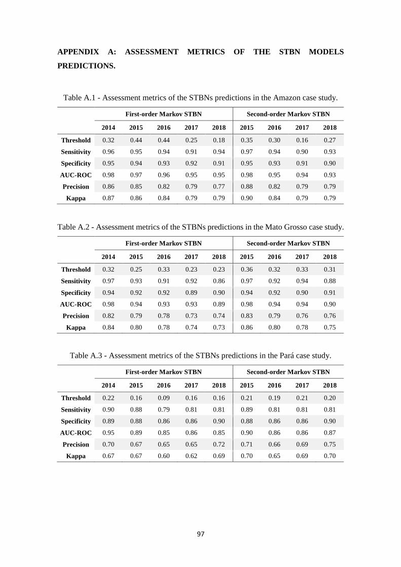
97
APPENDIX A: ASSESSMENT METRICS OF THE STBN MODELS
PREDICTIONS.
Table A.1 - Assessment metrics of the STBNs predictions in the Amazon case study.
First-order Markov STBN Second-order Markov STBN
2014 2015 2016 2017 2018 2015 2016 2017 2018
Threshold 0.32 0.44 0.44 0.25 0.18 0.35 0.30 0.16 0.27
Sensitivity 0.96 0.95 0.94 0.91 0.94 0.97 0.94 0.90 0.93
Specificity 0.95 0.94 0.93 0.92 0.91 0.95 0.93 0.91 0.90
AUC-ROC 0.98 0.97 0.96 0.95 0.95 0.98 0.95 0.94 0.93
Precision 0.86 0.85 0.82 0.79 0.77 0.88 0.82 0.79 0.79
Kappa 0.87 0.86 0.84 0.79 0.79 0.90 0.84 0.79 0.79
Table A.2 - Assessment metrics of the STBNs predictions in the Mato Grosso case study.
First-order Markov STBN Second-order Markov STBN
2014 2015 2016 2017 2018 2015 2016 2017 2018
Threshold 0.32 0.25 0.33 0.23 0.23 0.36 0.32 0.33 0.31
Sensitivity 0.97 0.93 0.91 0.92 0.86 0.97 0.92 0.94 0.88
Specificity 0.94 0.92 0.92 0.89 0.90 0.94 0.92 0.90 0.91
AUC-ROC 0.98 0.94 0.93 0.93 0.89 0.98 0.94 0.94 0.90
Precision 0.82 0.79 0.78 0.73 0.74 0.83 0.79 0.76 0.76
Kappa 0.84 0.80 0.78 0.74 0.73 0.86 0.80 0.78 0.75
Table A.3 - Assessment metrics of the STBNs predictions in the Pará case study.
First-order Markov STBN Second-order Markov STBN
2014 2015 2016 2017 2018 2015 2016 2017 2018
Threshold 0.22 0.16 0.09 0.16 0.16 0.21 0.19 0.21 0.20
Sensitivity 0.90 0.88 0.79 0.81 0.81 0.89 0.81 0.81 0.81
Specificity 0.89 0.88 0.86 0.86 0.90 0.88 0.86 0.86 0.90
AUC-ROC 0.95 0.89 0.85 0.86 0.85 0.90 0.86 0.86 0.87
Precision 0.70 0.67 0.65 0.65 0.72 0.71 0.66 0.69 0.75
Kappa 0.67 0.67 0.60 0.62 0.69 0.70 0.65 0.69 0.70
98
APPENDIX B: HYPOTHESIS TESTING FOR THE ASSESSMENT METRICS.
AUC-ROC, Precision, and Kappa metrics values for the first-order Markov STBN were
compared with the values of the same metrics for the second-order Markov STBN. To
test the hypothesis that there is a significant difference between the metrics of both
models, an independent t-test was performed for each one of those three metrics in each
case study. Considering 𝜇1 as the mean of the first-order Markov STBN assessment
metric, and 𝜇2 as the mean of the same assessment metric but for the second-order
Markov STBN, all independent t-tests performed had the null and alternative hypotheses
as follows:
𝐻0: 𝜇1 − 𝜇2 = 0, i.e., the difference between the means equals to zero,
𝐻𝑎: 𝜇1 − 𝜇2 ≠ 0, i.e., the difference between the means differs from zero.
Table B.1 shows the mean and standard deviation of each metric for both models as well
as the p-value obtained from the independent t-test with a significance level of 5%. One
can note that the p-value is greater than 0.05 in all t-tests performed, this states that the
difference found between the means is not statistically significant.
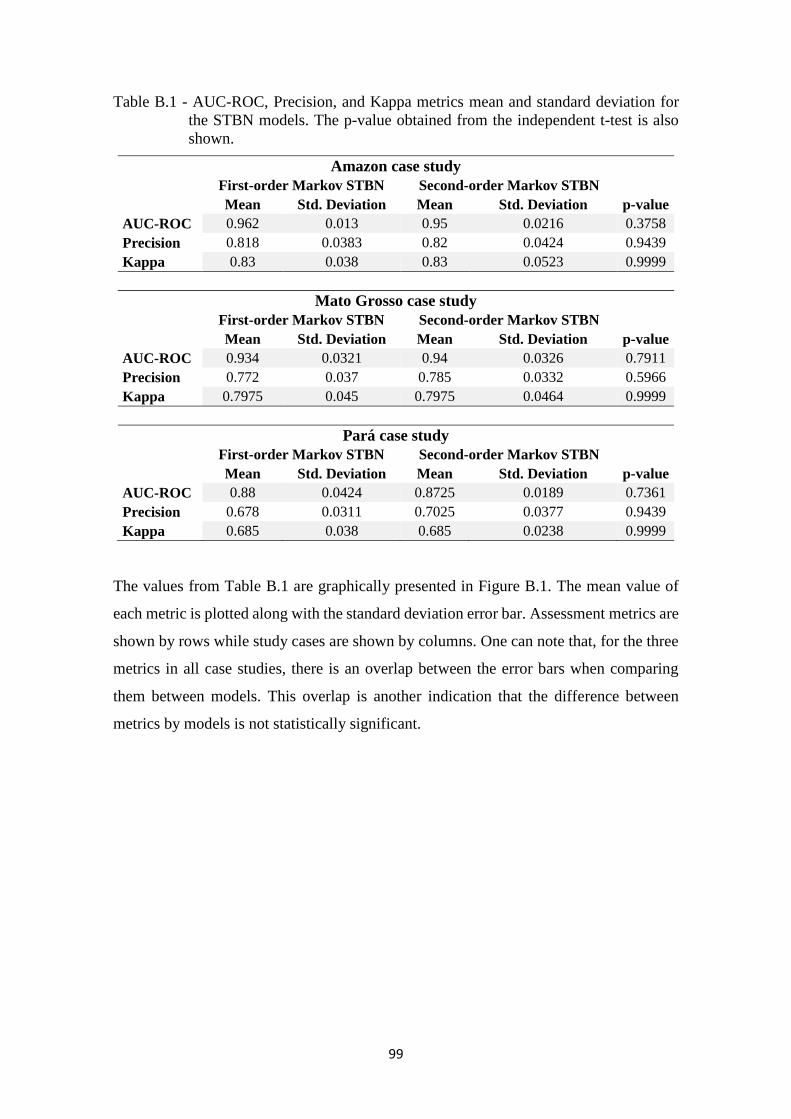
99
Table B.1 - AUC-ROC, Precision, and Kappa metrics mean and standard deviation for
the STBN models. The p-value obtained from the independent t-test is also
shown.
Amazon case study First-order Markov STBN Second-order Markov STBN
Mean Std. Deviation Mean Std. Deviation p-value
AUC-ROC 0.962 0.013 0.95 0.0216 0.3758
Precision 0.818 0.0383 0.82 0.0424 0.9439
Kappa 0.83 0.038 0.83 0.0523 0.9999
Mato Grosso case study First-order Markov STBN Second-order Markov STBN
Mean Std. Deviation Mean Std. Deviation p-value
AUC-ROC 0.934 0.0321 0.94 0.0326 0.7911
Precision 0.772 0.037 0.785 0.0332 0.5966
Kappa 0.7975 0.045 0.7975 0.0464 0.9999
Pará case study First-order Markov STBN Second-order Markov STBN
Mean Std. Deviation Mean Std. Deviation p-value
AUC-ROC 0.88 0.0424 0.8725 0.0189 0.7361
Precision 0.678 0.0311 0.7025 0.0377 0.9439
Kappa 0.685 0.038 0.685 0.0238 0.9999
The values from Table B.1 are graphically presented in Figure B.1. The mean value of
each metric is plotted along with the standard deviation error bar. Assessment metrics are
shown by rows while study cases are shown by columns. One can note that, for the three
metrics in all case studies, there is an overlap between the error bars when comparing
them between models. This overlap is another indication that the difference between
metrics by models is not statistically significant.
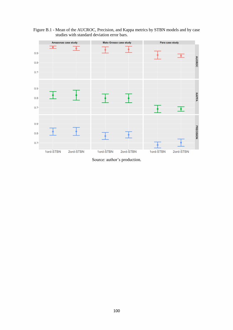
100
Figure B.1 - Mean of the AUCROC, Precision, and Kappa metrics by STBN models and by case
studies with standard deviation error bars.
Source: author’s production.


![Bayesian spatio-temporal epidemic models with applications ...arXiv:1403.1783v1 [stat.AP] 7 Mar 2014 Bayesian spatio-temporal epidemic models with applications to sheep pox C. Malesios1,](https://img.pdfslide.net/doc/110x75/5f315b202139fe2ba9185fef/bayesian-spatio-temporal-epidemic-models-with-applications-arxiv14031783v1.jpg)