Embed Size (px)
Citation preview
A SS FINITE ELEMENT APPROACH
AND VIBRATION ANALYSIS
ANISOTROPIC ELASTICITY
J. TINSLEY UlkN,
bY GERALD W. FLY and L. MAHADEVAN
TR-87-05
An Interim Technical Report to the
NAUTICS 81 SPACE ADMINISTRATION =ALL SPACE FLIGHT CENTER, AL
pertaining to Contract No. NAS 8-37283
October, 1987
Computational Mechanics Company, Inc. 4804 Avenue H Austin, Texas 78751
THE COIIPL7ATIOh'AL YECHAWCS COM?AM'. ISC.
- .
[NAS4-CR-119311) a XYBRID-STRESS FII.LI;TB N88- 197 84 ELEHENT APPROACH POE STRESS AND V I B R A 2 I O I ANALYSIS XU LIMBAB AMISOTROPIC BLASTXCITY
Sep., 1987 (Computational Plechanics Co.2 G3/39 0119639 Interim Technical Report, period endiny 3 9 . Unclas
*.,-
https://ntrs.nasa.gov/search.jsp?R=19880010400 2018-08-15T06:12:15+00:00Z
A HYBRID-STRESS FINITE ELEMENT APPROACH
FOR STRESS AND VIBRATION ANALYSIS
IN LINEAR ANISOTROPIC ELASTICITY
bY J. TINSLEY ODEN, GERALD W. FLY and L. MAHADEVAN
TR-87-05
An Interim Technical Report to the
NATIONAL AERONAUTICS & SPACE ADMINISTRATION MARSHALL SPACE FLIGHT CENTER, AL
pertaining to
Contract No. NAS 8-37283
October, 1987
/\ T H E C O \ I P t T A f l O S A L HECH4YICS C O V P A Y l , I \ C
Computational Mechanics Company, Inc. 4804 Avenue H Austin, Texas 78751
A HYBRID-STRESS FINITE ELEMENT APPROACH FOR STRESS AND VIBRATION ANALYSIS IN LINEAR ANISOTROPIC ELASTICITY
Abstract
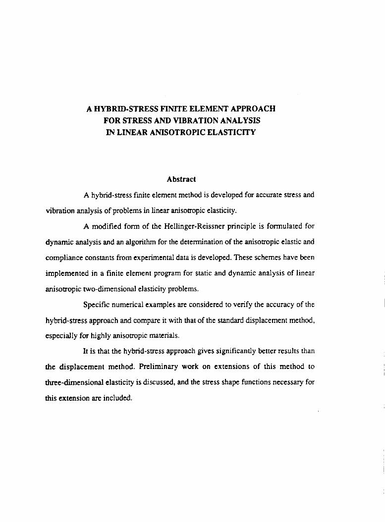
A hybrid-stress finite element method is developed for accurate stress and
vibration analysis of problems in linear anisotropic elasticity.
A modified form of the Hellinger-Reissner principle is formulated for
dynamic analysis and an algorithm for the detennination of the anisotropic elastic and
compliance constants from experimental data is developed. These schemes have been
implemented in a finite element program for static and dynamic analysis of linear
anisotropic two-dimensional elasticity problems.
Specific numerical examples are considered to verify the accuracy of the
hybrid-stress approach and compare it with that of the standard displacement method,
especially for highly anisotropic materials.
It is that the hybrid-stress approach gives significantly better results than
the displacement method. Preliminary work on extensions of this method to
three-dimensional elasticity is &scussed, and the stress shape functions necessary for
this extension are included.
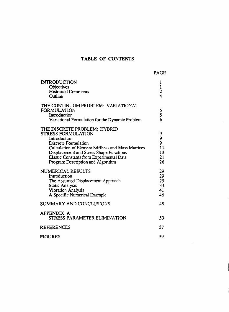
TABLE OF CONTENTS
PAGE
INTRODUCIION Objectives Historical Comments Outline
THE CONTINUUM PROBLEM: VARIATIONAL FORMULATION
Introduction Variational Formulation for the Dynamic Problem
THE DISCRETE PROBLEM: HYBRID STRESS FORMULATION
Introduction Discrete Formulation Calculation of Element Stiffness and Mass Matrices Displacement and Stress Shape Functions Elastic Constants from Experimental Data Program Description and Algorithm
NUMERICAL RESULTS Introduction The Assumed-Displacemen t Approach Static Analysis Vibration Analysis A Specific Numerical Example
SUMMARY AND CONCLUSIONS
APPENDIX A STRESS PARAMETER ELIMINATION
1 1 2 4
5 5 6
9 9 9 11 13 21 26
29 29 29 33 41 46
48
50
REFERENCES 57
FIGURES 59
INTRODUCTION
Objectives Stress-hybrid finite elements are developed for the study of equilibrium
and vibration problems in two- and three-dimensional linear anisotropic elasticity. It has been observed that standard displacement-type finite element
methods may produce very poor approximations of stresses, displacements, natural frequencies and mode shapes for strongly anisotropic elastic bodies, such as structures composed of single metallic crystals. The possibility of resolving these deficiencies by using elements based on assumed stresses is explored in this study.
Further motivation of this work is a result of problems faced in the analysis of single crystal turbine blades subjected to very large centrifugal and fluid forces as in the fuel pump for the space shuttle main engine, where the high degree of anisotropy in the crystal leads to very poor results using standard displacement-type finite elements.
The static problem is solved using a form of the Hellinger-Reissner energy functional where the displacements and stresses may be independently interpolated. To accommodate anisotropic materials, an algorithm for computing the elasticity and compliance constants from experimental data is developed. For the analysis of vibration problems, a special Hellinger-Reissner-type variational principle, valid for dynamic problems in linear elasticity, is also developed. The eigen pairs are extracted using a standard subroutine package.
Some numerical examples in two-dimensional linear elasticity are chosen to verify the accuracy of the assumed-stress approach and compare the results obtained therein with those obtained using the standard displacement-type finite element method. Specifically, end loaded cantilever beams are chosen to simulate in a crude way turbine blades without unnecessary complexity in geometry or loading. Various degrees of anisotropy are assumed for the materials and the results obtained .
1
are compared with analytic solutions whenever the latter are available. It is observed that there is a significant difference in the results obtained
using conventional and assumed-stress finite elements, especially as the degree of anisotropy increases and the orientation of the local axes changes with respect to the global axes. The hybrid-stress elements behave very consistently and give good approximations of the stresses, natural frequencies and mode shapes, independent of the degree of anisotropy and element orientation while displacement elements are found to be sensitive to changes in material propemes and element orientation.
Historical Comments The mathematical, and practical aspects of assumed-displacement finite
elements have been the subject of extensive research for many years. As a result of the sound theoretical fundamentals, the existence of a good mathematical basis and the ease of element formulation has resulted in the widespread use of such formulations. Indeed, most general-purpose computer programs employ the classical dxplacemen t approach.
However, the displacement finite element model has some shortcomings which are evident in constrained media problems such as those involving incompressible materials and plate elements requiring only Co continuity interpolations (instead of the more difficult C1 continuity interpolations that are based on thin plate theories). In these cases, "element locking" may occur as a result of very snff solutions that arise as the constraint condition is approached. Reduced integration or selective-reduced integration can alleviate the problem partially, but an undesirable consequence may be the appearance of unwanted spurious energy modes.
An alternative approach is to use the hybrid-stress model initiated by Pian [ 11, who independently interpolated intra-element stresses and compatible boundary displacements, using a variational principle akin to the principle of minimum
2
complementary energy. The ability to interpolate the stresses independently led to the solution of
problems in fracture mechanics [2], thick, laminated composite materials [3], and constrained media (nearly incompressible materials) [4]. However, the versatility of independently interpolating stresses also leads to serious numerical difficulties.
A minimum number of stress parameters is required to ensure correct stiffness rank and care has to be taken to make sure that the stiffness is invariant under simple transformations of the coordinates, and to prevent the entry of spurious energy modes into the element stiffness. Work on a systematic approach to the selection of these stress parameters has been done by Spilker, Maskeri and Kania [SI (for complete stress polynomials) and recently by Rubinstein, Punch and Atluri [ 61 and Punch and Atluri [7,8] using group theoretical methods to minimize the number of stress parameters and still satisfy rank and invariance conditions, for both two- and three-dimensional isoparametric elements.
In addition, Pian and Chen [12] as well as Pian, Chen and Kang [lo] have proposed new formulations for the hybrid-stress method, where the Hellinger-Reissner principle is used to generate elements in which equilibrium is not satisfied a-priori. Stress equilibrium is introduced in these methods by means of Lagrange multipliers. Another formulation, following the Hu-Washizu principle, is also suggested in [ 191.
Outline Following a brief discussion of some variational principles, the variational
formulation for dynamic problems in linear anisotropic elasticity, based on a Hellinger-Reissner-type principle, is developed.
Our third section, entitled "The Discrete Problem: Hybrid Stress Formulation", deals with the finite element discretization of the continuum problem, and the calculation of the element stiffness and mass matrices. A separate section is
3
devoted to the development of an algorithm for determining the elastic and compliance constants from experimental data in the form of Young's moduli and Poisson's ratios in different directions.
In a further section, some numerical examples are presented and the hybrid-stress rtsults are compared with those obtained using the displacement model. Problems involving materials with varying degrees of anisotropy are also considered to compare the two models.
Conclusions and suggestions for further work, especially in three dimensions, are discussed in our final section.
4
THE CONTINUUM PROBLEM: VARIATIONAL FORMULATION
Introduction In this section, following a brief description of some general variational
principles, a modified form of the Hellinger-Reissner principle valid for dynamic problems in linear elasticity is developed.
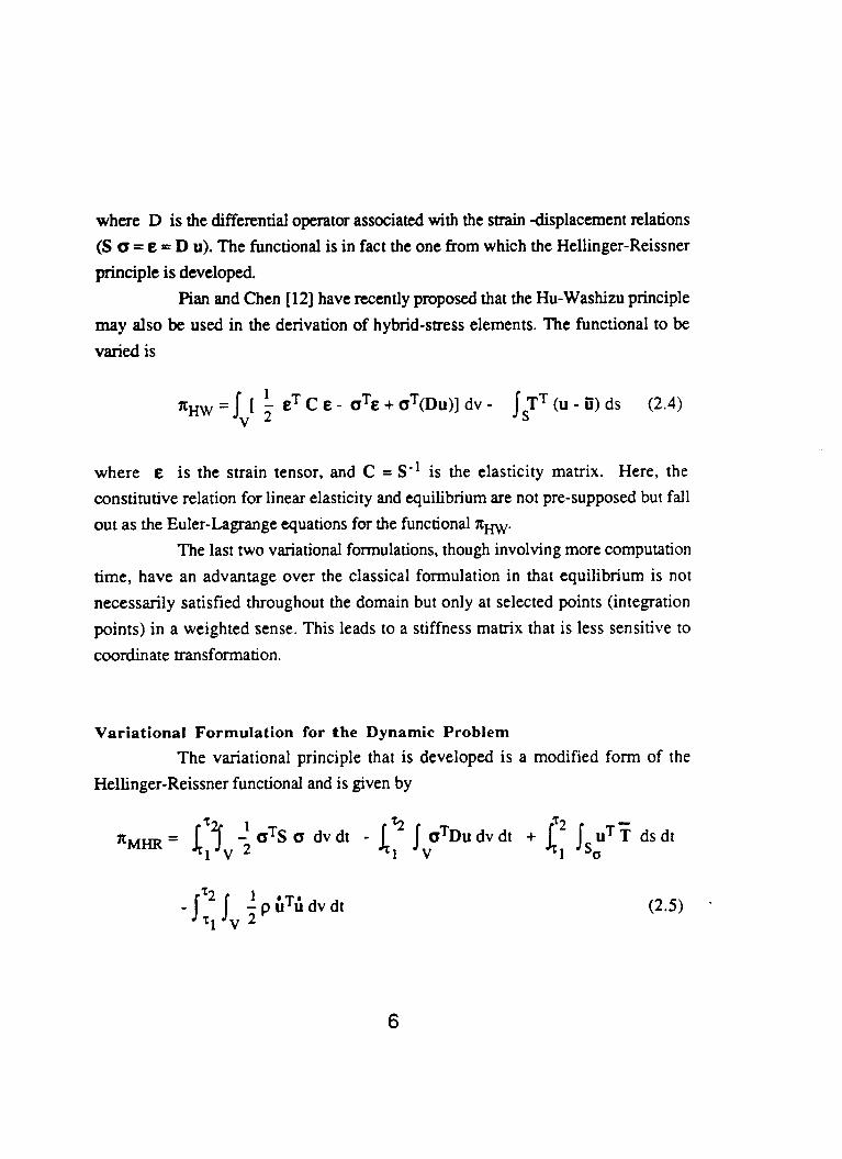
The classical stress-hybrid models for finite element analysis [ 13 are derived from the principle of minimum complementary energy for which the functional to be varied is given by
7tc = j a T S a d v - j T T n d s v 2 SU
where d is the stress tensor (here a vector of stress components) which satisfies the equilibrium equation DT a + f = 0, fare the body forces, S is the compliance matrix, u are the prescribed displacements on the boundary S,, and T is the surface traction vector, where DT is the mamx divergence operator.
Alternatively, the equilibrium conditions may be regarded as a constraint and a term of the form hT (DT a + f) can be introduced into the functional with the Lagrangian multipliers h being identified with the displacement field. Then,
Integrating the second tern by parts, we get
1 - oT S Q dv - aT(Du) dv - TT (u - 0 ) ds V SU
(2.3)
5
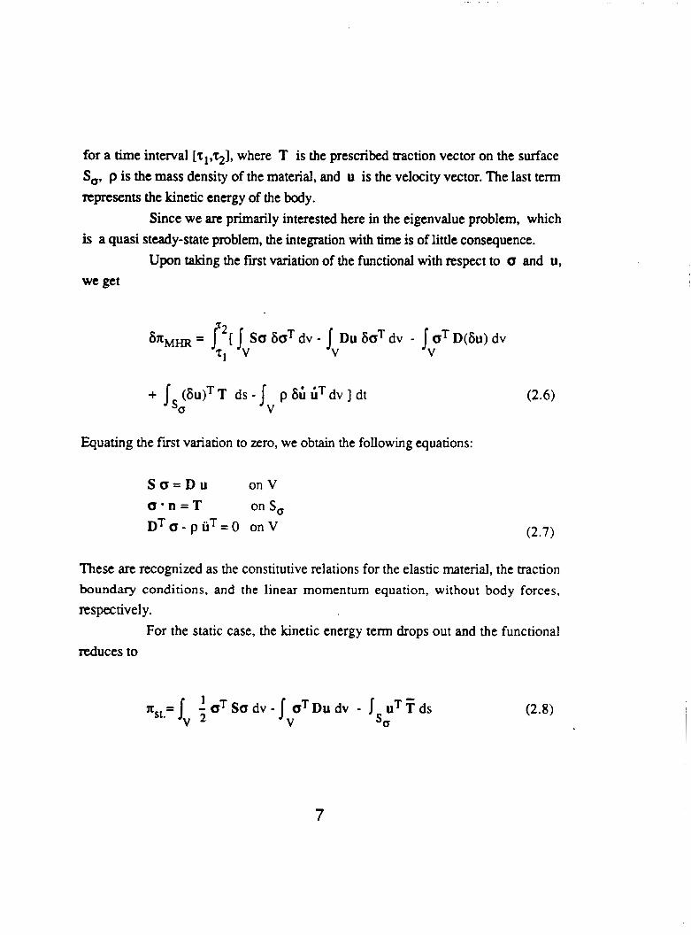
where D is the differential operator associated with the strain displacement relations (S G = & = D u). The functional is in fact the one from which the Hellinger-Reissner principle is developed.
Pian and Chen [12] have recently proposed that the Hu-Washizu principle may also be used in the derivation of hybrid-stress elements. The functional to be varied is
1 x.w=Jv [ - ET C E - bT& + aT(Du)] dv - IFT (u - 6) ds (2.4)
where E is the strain tensor, and C = S-l is the elasticity matrix. Here, the constitutive relation for linear elasticity and equilibrium are not pre-supposed but fall out as the Euler-Lagrange equations for the functional nHw.
The last two variational formulations, though involving more computation time, have an advantage over the classical formulation in that equilibrium is not necessarily satisfied throughout the domain but only at selected points (integration points) in a weighted sense. This leads to a stiffness mamx that is less sensitive to coordinate transformation.
Variational Formulation for the Dynamic Problem
The variational principle that is. developed is a modified form of the Hellinger-Reissner functional and is given by
aTDu dv dt + [: Is u T T ds dt - r: I, 0
1 x M m = L:7v -- aTS a dv dt
- J:jv f p h T 3 d v d t (2.5) *
6
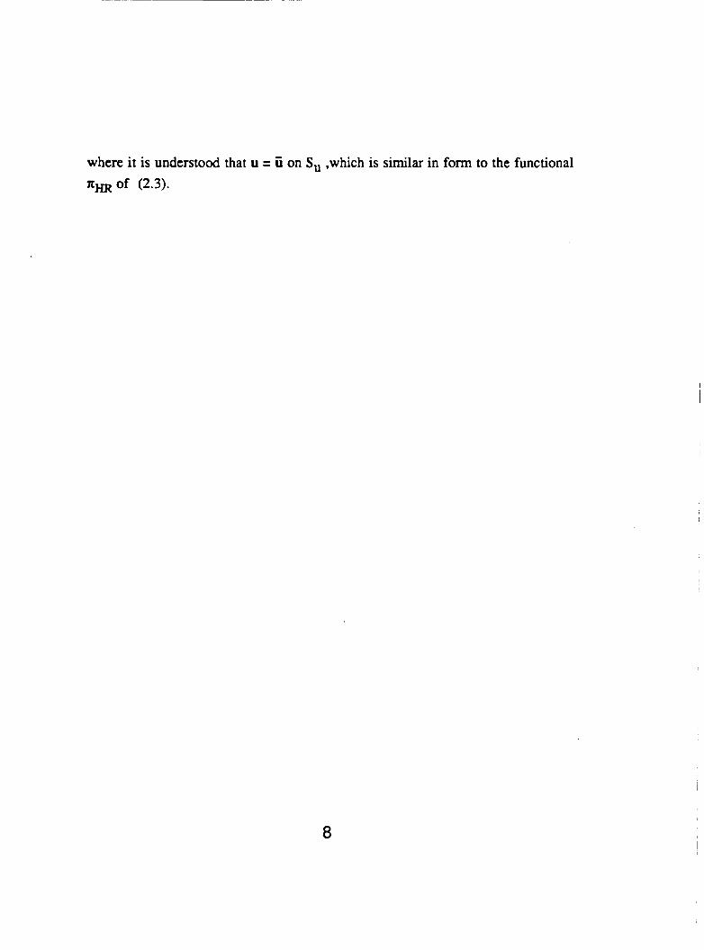
for a time interval [9,~~], where T is the prescribed traction vector on the surface Sa, p is the mass density of the material, and u is the velocity vector. The last term represents the kinetic energy of the body.
Since we arc primarily interested here in the eigenvalue problem, which is a quasi steady-state problem, the integration with time is of little consequence.
Upon taking the first variation of the functional with respect to Q and u, we get
8xMm = r2[ Sa 6aT dv - Du 6aT dv - aT D(6u) dv V v TI
( 6 ~ ) ~ T ds - p 6; iT dv 3 dt V
Equating the first variation to zero, we obtain the following equations:
S o = D u on V a * n = T on So ~ T a - p i i T = ~ o n v (2.7)
These are recognized as the constitutive relations for the elastic material, the traction boundary conditions, and the linear momentum equation, without body forces, respectively.
For the static case, the kinetic energy term drops out and the functional reduces to
1 - a T S a d v - j oTDudv - u T T d s
V so
7
where it is understood that u = ii on Su ,which is similar in form to the functional I C ~ of (2.3).
8
THE DISCRETE PROBLEM: HYBRID STRESS FORMULATION
Introduction In this section, we discuss the discrete hybrid-stress approximation to the
continuous problem defined in the previous section. A detailed account of the calculations of the stiffness and mass matrix are given, along with derivations of the stress shape functions for both two- and three-dimensional finite elements.
Following this, an extended discussion of the algorithm for the determination of the elasticity and compliance constants from experimental data is presented.
The section ends with a note on the algorithm used to write a general finite element program using either displacement or hybrid-stress elements to solve static and dynamic problems in two-dimensional linear elasticity.
Discrete Formulation The functional to be minimized in the continuum problem is given by
If the continuum is discretized into n elements then the discrete form of the continuous functional is given by
where R, represents the volume of the elements, and aR, boundary over which the surface traction is prescribed.
represents the m
9
As shown in the previous section, the above functional (for the static case) reduces to the conventional assumed-stress model when the stresses are forced to satisfy equilibrium (in the absence of body forces). This was noted by Pian [ 13 who also demonstrated its equivalence to the Hellinger-Reissner functional with the smsses satisfying equilibrium.
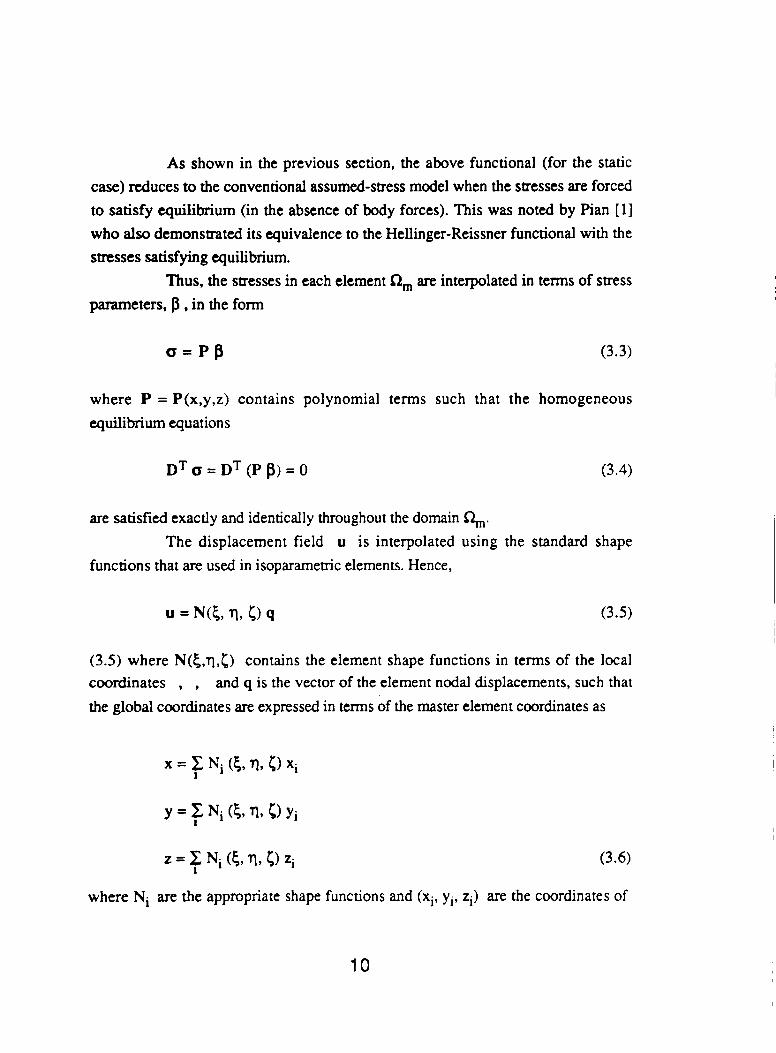
Thus, the stresses in each element R, are interpolated in terms of stress parameters, p , in the form
a = P P (3.3)
where P = P(x,y,z) contains polynomial terms such that the homogeneous equilibrium equations
are satisfied exactly and identically throughout the domain %.
functions that are used in isoparamemc elements. Hence, The displacement field u is interpolated using the standard shape
(3.5) where N(k,q,C) contains the element shape functions in terms of the local coordinates , , and q is the vector of the element nodal displacements, such that the global coordinates are expressed in terms of the master element coordinates as
z = C Nj (5, V, {> zj (3.6) 1
where Ni are the appropriate shape functions and (xi, yi, zi) are the coordinates of
10
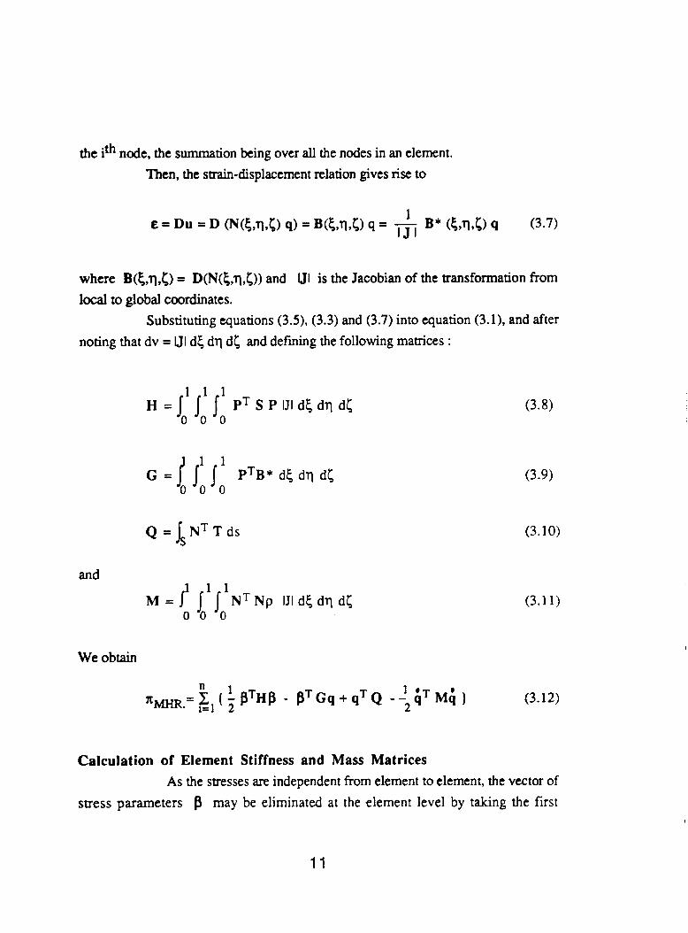
the ith node, the summation being over ~.IJ the nodes in an element. Then, the strain-displacement relation gives rise to
where B(C,q,r) = D(N(t,q,r)) and UI is the Jacobian of the transformation from local to global coordinates.
Substituting equations (3.5), (3.3) and (3.7) into equation (3.1), and after noting that dv = UI dc dq dc and defining the following matrices :
1 1 1
0 0 0 H =I PT S P IJI dk dq dc
1 1
0 0 0 G = { PTB* dc dq dc
(3.8)
(3.9)
Q = i N T T d s (3.10)
and
M = ( I I J I N T Np IJI dc dq d r 0 0 0
(3.1 1)
We obtain
Calculation of Element Stiffness and Mass Matrices As the stresses are independent from element to element, the vector of
may be eliminated at the element level by taking the first stress parameters
11
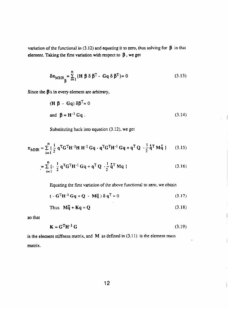
variation of the functional in (3.12) and equating it to zero, thus solving for element. Taking the fmt variation with respect to p , we get
in that
Since the p's in every element are arbitrary,
(H p - Gq) 6BT=0
and p = H - ' G q . (3.14)
Substituting back into equation (3.12), we get
" 1 1 2 2
= C ( - qTGTH-'H H-' Gq - qTGTH-' Gq + qT Q - - ;IT M 4 ) (3.15) i= 1
" 1 1 b = c ( - %qTGTH-IGq+qTQ - -qTMq 2 ) i= 1
(3.16)
Equating the first variation of the above functional to zero, we obtain
Thus M c + K q = Q (3.18)
so that
K = GTH-' G (3.19)
is the element stiffness matrix, and M as defined in (3.1 1) is the element mass
UMtriX.
12
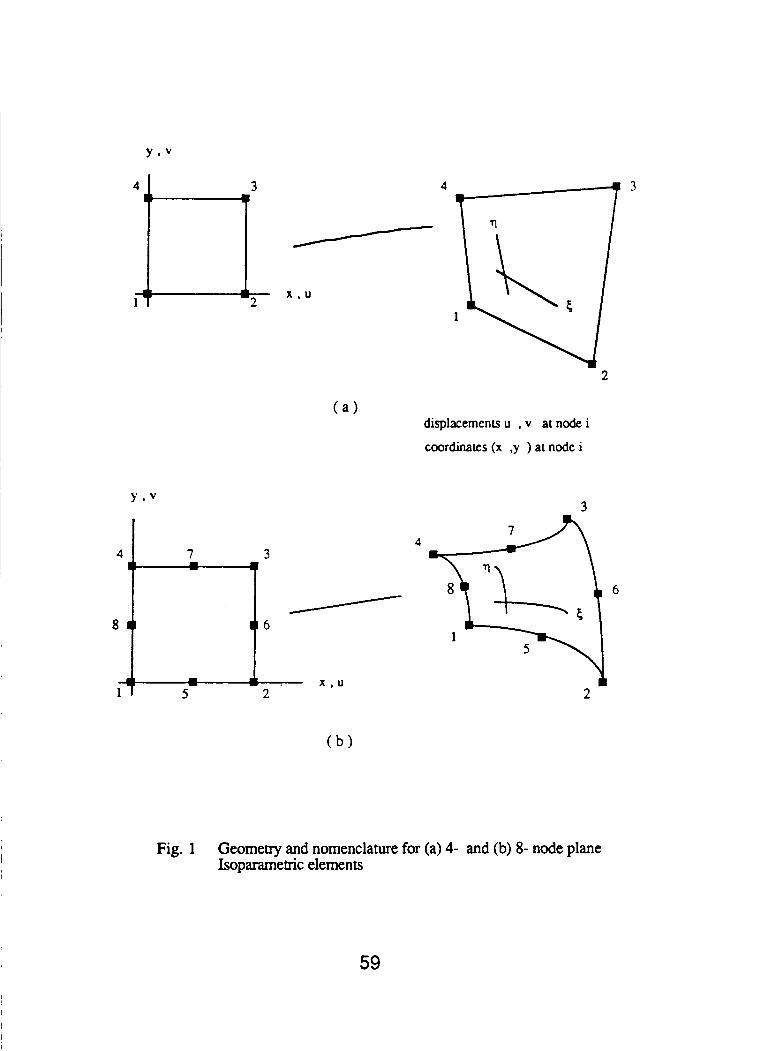
Displacement and Stress Shape Functions The displacement functions are the same as those i n the
assumed-displacement model. For two-dimensional elements, two kinds of elements are chosen: the four-noded bilinear quadrilateral elements and the eight-noded quadratic quadrilateral elements (serendipity elements). These are shown in Figure 1.
Since the stresses inside each element are interpolated independently of the displacement, a multitude of choices exists for the stress polynomials that constitute the P matrix. A number of factors govern the choice of these polynomials, however.
In the assumed displacement model, the stiffness mamx is automatically free from zero-energy or kinematic deformation (rigid body) modes, and is invariant with respect to simple transformations of the referencdnatural coordinates.
In addition to the advantages of a hybrid-stress model, viz., accurate stress evaluation and a stiffness mamx that is not overly rigid, it is important that the inherent properties of the assumed displacement model, namely, invariance with respect to coordinate transformations and freedom from rigid body modes of the stiffness matrix are preserved when the stress polynomials are chosen, for the hybrid-stress model to have any real use in finite element analysis.
To avoid the presence of kinematic deformation modes, it is necessary that the stiffness mamx satisfy the following condition that determines its minimum rank (Pian [l] , and Atluri and Punch [7]).
If the number of stress parameters per element is s , the mamx H defined in equation (3.8) will be positive-definite and of rank s (as the energy density functional is always positive-definite). The rank of the stiffness matrix is then determined by that of the G mamx as defined in equation (3.9).
The order of the G mamx is s x d where d is the number of generalized degrees of freedom per element. If there are r rigid body modes per element, then at best the rank of the G matrix is given by min(s, d-r), and as a consequence the rank of the stiffness mamx is given by min(s, d-r).
Since any stiffness matrix should include all the rigid body modes of the element, the rank of K in equation (3.19) should be d-r.
13
I
For a linear quadrilateral element, the minimum number of stress parameters is
s = d-r = 2 x 4 - 3 = 5 .
After satisfying equilibrium, the 9 P field reduces to a seven parameter linear stress approximation given by
aq = P3 + P4 5 + P7 rl (3.23)
where 6 and rl are the local coordinates as shown in Fig. 1.
of stress parameters is For a quadratic quadrilateral element with 8 nodes, the minimum number
s = d-r = 2 x 8 - 3 = 1 3 .
Choosing a complete cubic stress approximation with 30 p's, upon enforcing equilibrium we get the following 18 parameter stress field :
PRECElDING PAGE BLANK NOT FILMED 15
To reduce the number of parameters still further, we impose the Beltrami-Michell compatibility conditions for isotropic materials or the stress field. For the more general case of plane strain, in addition to equilibrium, this requires that (Sokolnikoff [ 1 11)
v2 (66 + Oq) = 0 (3.25)
when there are no body forces.
renumbering, we get a 15 P stress field given by Substituting (3.24) into (3.25), eliminating any redundant P's and
However, as mentioned earlier, the Beltrami-Michell equations in the form (3.25) are valid only for isotropic materials. For the general case of anisotropy, the compatibility conditions as expressed in terms of the strain are given by
V X V X E = O (3.27)
16
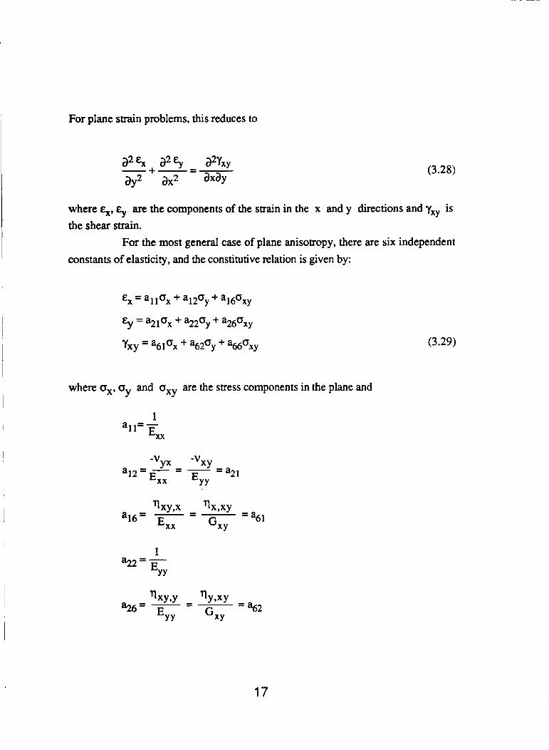
For plane strain problems, this reduces to
(3.28)
where %, ~y are the components of the strain in the x and y directions and y,, is the shear strain.
For the most general case of plane anisotropy, there are six independent constants of elasticity, and the constitutive relation is given by:
&x = a120y + a160xy
Ey = a21ox + a22oy + a26oxy
yx y = a6 1 Ox + a620y +
where ox, o and oxy are the stress components in the plane and Y
1
-V -vx y
E,, = a21 yx - - - -
l2 = E,, a
1 %=-
E,,
(3.29)
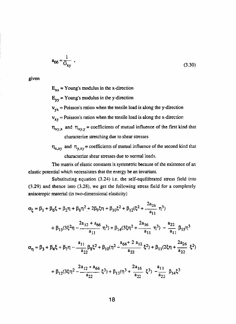
1 %=- '
GXY (3.30)
given
En = Young's modulus in the x-direction
E,, = Young's modulus in the y-direction
= Poisson's ration when the tensile load is along the y-direction
= Poisson's ration when the tensile load is along the x-direction "yx
v,Y
qxy,x and qxyVy = coefficients of mutual influence of the first kind that
characterize stretching due to shear stresses
and qy,xy = coefficients of mutual influence of the second kind that
characterize shear stresses due to n o d loads. qxYY
The matrix of elastic constants is symmetric because of the existence of an elastic potential which necessitates that the energy be an invariant.
Substituting equation (3.24) i.e. the self-equilibrated stress field into (3.29) and thence into (3.28), we get the following stress field for a completely anisotropic material (in two-dimensional elasticity)
18
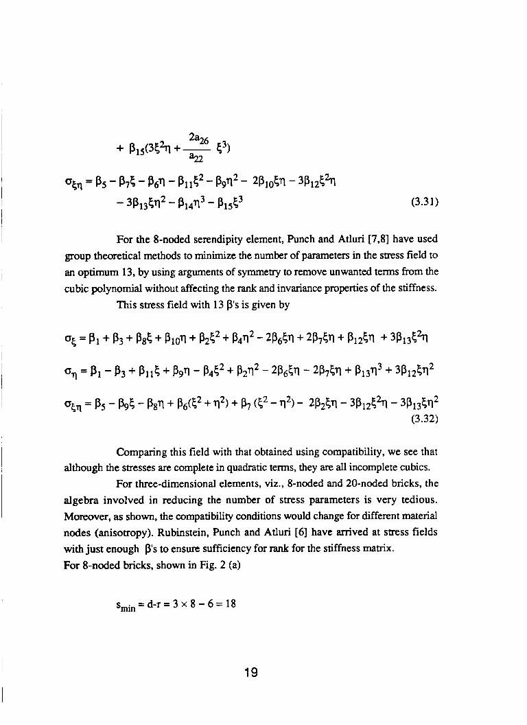
For the 8-noded serendipity element, Punch and Atluri [7,8] have used group theoretical methods to minimize the number of parameters in the stress field to an optimum 13, by using arguments of symmetry to remove unwanted terms from the cubic polynomial without affecting the rank and invariance properties of the stiffness.
This stress field with 13 P's is given by
Comparing this field with that obtained using compatibility, we see that although the stresses are complete in quadratic terms, they are all incomplete cubics.
For three-dimensional elements, viz., 8-noded and 20-noded bricks, the algebra involved in reducing the number of stress parameters is very tedious. Moreover, as shown, the compatibility conditions would change for different material nodes (anisotropy). Rubinstein, Punch and Atluri [6] have anived at stress fields with just enough p's to ensure sufficiency for rank for the stiffness matrix.
For 8-noded bricks, shown in Fig. 2 (a)
smin = d-r = 3 x 8 - 6 = 18
19
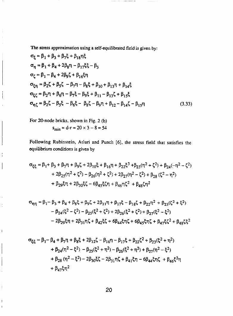
(3.33)
For 20-node bricks, shown in Fig. 2 (b) smi, = d-r = 20 x 3 - 8 = 54
Following Rubinstein, Atluri and Punch [6 ] , the stress field that satisfies the equilibrium conditions is given by
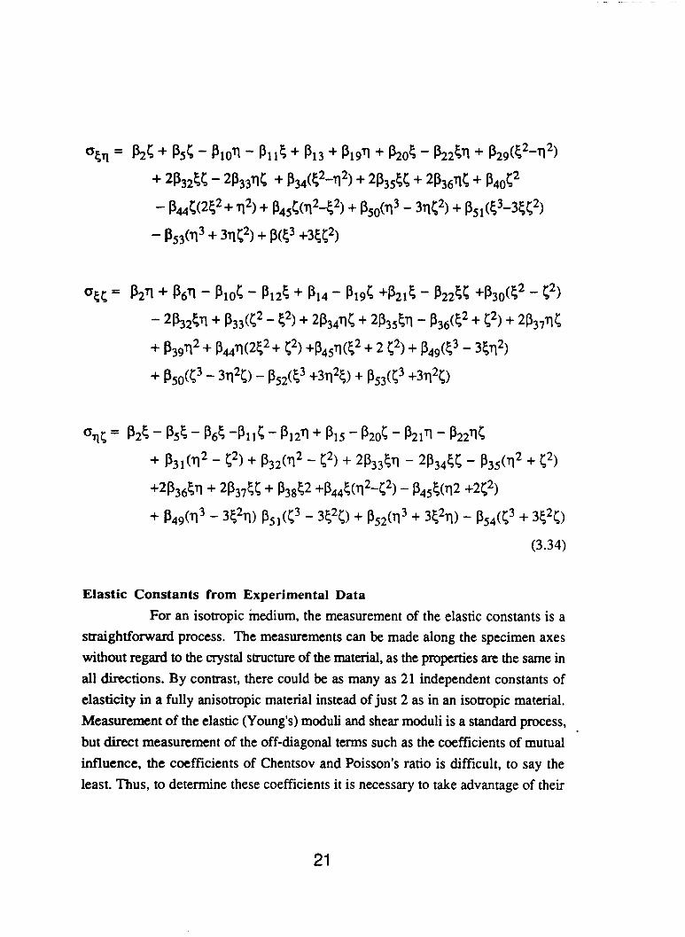
Elastic Constants from Experimental Data For an isotropic medium, the measurement of the elastic constants is a
straightforward process. The measurements can be made along the specimen axes without regard to the crystal structure of the material, as the properties are the same in all directions. By contrast, there could be as many as 21 independent constants of elasticity in a fully anisotropic material instead of just 2 as in an isotropic material. Measurement of the elastic (Young’s) moduli and shear moduli is a standard process, but direct measurement of the off-diagonal terms such as the coefficients of mutual influence, the coefficients of Chentsov and Poisson’s ratio is difficult, to say the least. Thus, to determine these coefficients it is necessary to take advantage of their
21
internlationship under rotation. If the measurements of the material properties are taken along an
orthogonal coordinate system which is rotated with respect to the primary material axes, the compliance (or elastic) matrix with respect to the rotated coordinate system will be a transformation of the matrix with respect to the original coordinate system dependent solely on the direction cosines of the rotation of the coordinate system from the primary material axes to the global coordinate axes.
In the realm of linear isothermal elasticity, there are a maximum of 21 independent constants. Hence, any quantity that is measured in the rotated (global) frame of reference is a function of all 21 components of the compliance matrix in the unrotated frame. For a unique determination of the coefficients of the unrotated compliance matrix, 21 independent equations in 21 unknowns are required. These could be obtained by the measurement of the same quantity in 21 independent directions or by measuring more than one quantity in many independent directions so that there are at least 21 independent equations. Thus, a least square fit can be carried out on the data to determine the best approximation to the elastic constants in the compliance matrix.
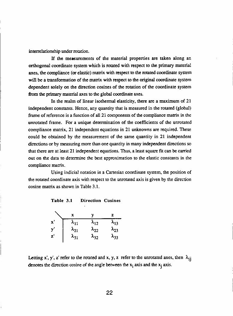
Using indicial notation in a Cartesian coordinate system, the position of the rotated coordinate axis with respect to the unrotated axis is given by the direction cosine matrix as shown in Table 3.1.
Y' 2'
Table 3.1 Direction Cosines
+21 +22 +23
'3 1 '32 h33
\ x Y Z
X' '11 h12 '13
LetMg x', y', z' refer to the rotated and x, y, z refer to the unrotated axes, then Aij denotes the direction cosine of the angle between the xi axis and the Xj axis.
22
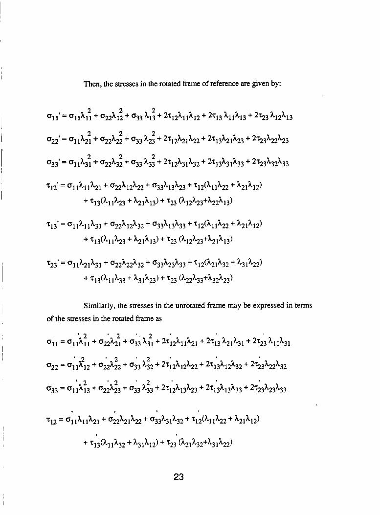
Then, the stresses in the rotated frame of reference are given by:
Similarly, the stresses in the unrotated frame may be expressed in terms of the stresses in the rotated frame as
' I I I
'12 = O1 l'llhl + O22%1h2 033'31'32 + '12('11%2 %1'12)
23
I I
I I 1 I
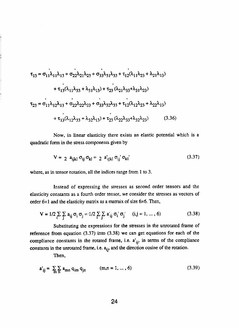
Now, in linear elasticity there exists an elastic potential which is a quadratic form in the stress components given by
(3.37)
where, as in tensor notation, all the indices range from 1 to 3.
Instead of expressing the stresses as second order tensors and the elasticity constants as a fourth order tensor, we consider the stresses as vectors of order 6x1 and the elasticity matrix as a matraix of size 6x6. Then,
V = 1/2 C aij oi oj =,1/2 C C a I i j oil aj' (iJ = 1, ... , 6) (3.38)
Substituting the expressions for the stresses in the unrotated frame of reference from equation (3.37) into (3.38) we can get equations for each of the compliance constants in the rotated frame, i.e. atij, in terms of the compliance constants in the unrotated frame, i.e. aij, and the direction cosine of the rotation.
1 J 1 J
Then,
24
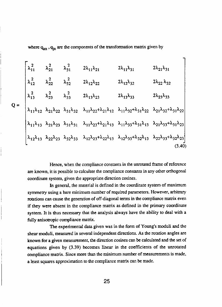
where qim , qjn are the components of the transformation matrix given by
Q =
p1 ',2, '3: 2'1 1'21
'?2 '22 A322 2' 12'22 2
'323 2'13'23
2'11'31
2'12'32
2'13'33
'2 1 '3 1
2'22 '32
2'23'33
'11'12 '21'22 '31'32 '11'22+'21'12 '11'32S'31'22 '21'32+'31'22
'1 1x1 3 '21 '23 '3 1 '3 1 '1 1 h23+x21h1 3 ' 1 1 '33+'3 1'13 '21 '33+'3 1'23
'1 2' 13 '&23 '32'33 12h23+x22h 13 12'33+'32' 13 '22'33+'32'21
(3.40)
Hence, when the compliance constants in the unrotated frame of reference are known, it is possible to calculate the compliance constants in any other orthogonal coordinate system, given the appropriate direction cosines.
In general, the material is defined in the coordinate system of maximum symmetry using a bare minimum number of required parameters. However, arbitrary rotations can cause the generation of off-diagonal terms in the compliance matrix even if they were absent in the compliance mamx as defined in the primary coordinate system. It is thus necessary that the analysis always have the ability to deal with a fully anisotropic compliance matrix.
The experimental data given was in the form of Young's moduli and the shear moduli, measured in several independent directions. As the rotation angles are known for a given measurement, the direction cosines can be calculated and the set of equations given by (3.39) becomes linear in the coefficients of the unrotated compliance matrix. Since more than the minimum number of measurements is made, a least squares approximation to the compliance matrix can be made.
25
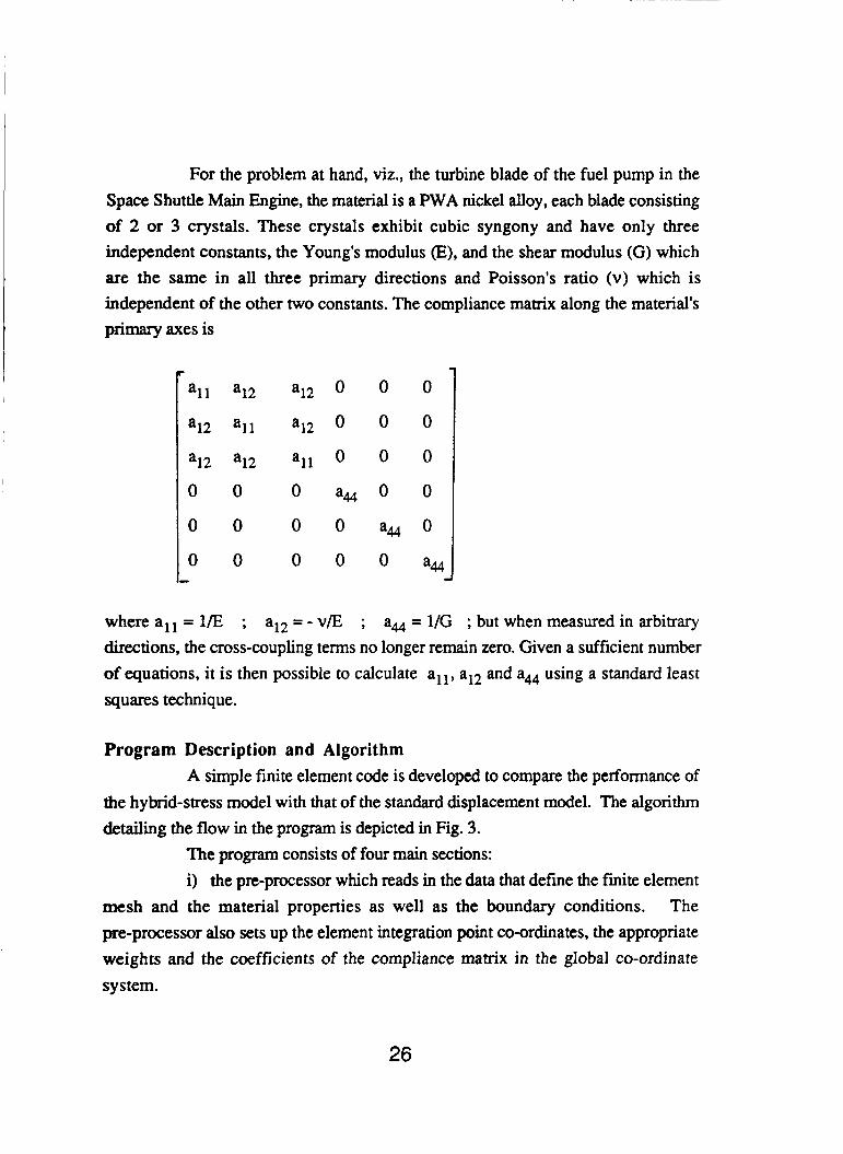
For the problem at hand, viz., the turbine blade of the fuel pump in the Space Shuttle Main Engine, the material is a PWA nickel alloy, each blade consisting of 2 or 3 crystals. These crystals exhibit cubic syngony and have only three independent constants, the Young's modulus (E), and the shear modulus (G) which are the same in all three primary directions and Poisson's ratio (v) which is independent of the other two constants. The compliance matrix along the material's primary axes is
a12 al l a12 0 0 0
a12 a12 all O O 0 0 0 0 a , O 0
0 0 0 0 a , O
0 0 - where all = 1/E ; aI2 = - v/E ; aU = 1/G ; but when measured in arbitrary directions, the cross-coupling terms no longer remain zero. Given a sufficient number of equations, it is then possible to calculate all, aI2 and a44 using a standard least squares technique.
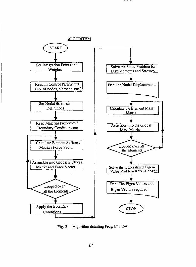
Program Description and Algorithm A simple finite element code is developed to compare the performance of
the hybrid-stress model with that of the standard displacement model. The algorithm detailing the flow in the program is depicted in Fig. 3.
The program consists of four main sections: i) the pre-processor which reads in the data that define the finite element
mesh and the material properties as well as the boundary conditions. The pre-processor also sets up the element integration point co-ordinates, the appropriate weights and the coefficients of the compliance matrix in the global co-ordinate system.
26
ii) the processor which calculates the individual element stiffness matrices as in equation (3.19) and assembles them to form a global stiffness matrix. It also calculates the individual force vectors and assembles them to form a global force vector. The processor then enforces the various boundary conditions, viz., prescribed displacement, surface traction and nodal forces, and finally solves for the unknown nodal displacements using a standard solver.
iii) the post-processor which calculates the stresses in each element once the nodal displacements are known. Unlike in the standard displacement model, where the strains are calculated first and then the stresses are obtained by using the stress-strain law, in the hybrid model, the stresses are calculated directly using equation (3.14), i.e.
= H" G q (3.14)
where the q's are the generalized nodal displacements in an element. Once the p's are known, the stresses are given as
a = P $ (3.3)
and are calculated at the Gauss points of integration. iv) the eigensolver, which sets up the element mass matrices as in
equation (3.1 l), assembles them to form a global mass mamx, and after weighting
the diagonal terns that correspond to prescribed displacement boundary conditions, calls a generalized eigensolver subroutine to calculate the eigen-pairs for the specified problem.
The Eigensolver used for these calculations was based on the Householder scheme.
The main feature of the complete code is that even though it has been set up to solve 2-dimensional static and dynamic problems, it is possible to solve 3-dimensional problems by making only minor modifications.
The number of degrees of freedom per node may be easily changed by means of a parameter statement, and the addition of 3-dimensional shape functions,
27
for displacements and stresses as well as Gaussian integration can make this program completely general.
28
NUMERICAL RESULTS
Introduction In this section, initially, a brief discussion of the standard
displacement model is presented, since it is used as a yardstick of comparison for the hybrid-stress model. The primary differences between the two schemes of analysis are also highlighted.
Following this, some examples for the statically loaded case are studied, with an emphasis on the displacements and stresses in a cantilever beam subjected to an end shear. Both hybrid-stress and displacement finite elements are used to analyze beams that are isotropic and anisotropic.
Then, an eigenvalue analysis of the cantilever beams is carried out to determine the first few natural frequencies and mode shapes, using both models for isotropic and anisotropic materials.
All the results are compared to analytical solutions whenever the latter are available.
The Assumed Displacement Approach
approach is alcin to the principle of minimum potential energy and is of the form The variational principle that is used in the standard displacement
22 - jZl E ds dt (4.1)
when there are no body forces, where
e = the strain tensor
29
c = the elasticity tensor = S-1
u = prescribed displacement on the boundary S,
T = prescribed traction on the boundary S,
- -
S, U S, = aV , the total boundary.
On taking the first variation of the functional given in (4.1) and
equating it to zero, we get the equations of motion and the traction boundary
condition, provided that the variation in the displacement 6u is zero on the boundary
Su , where the displacements are prescribed, i.e.
p; - D% = o on v u = u on S,
0 . n = T on S,
- - (4.2)
If the continuum is divided into n discrete elements, then the
discrete foxm of the functional xpE is given by
1 22 1 -i [ I" 2 p i T ; d v d t + 2 - E ~ C E d v d t 'tPE - i=l .rl R, 21
where R, represents the volume of the element and aR, is the part of the boundary of the element that has either prescribed displacement or prescribed traction.
30
As the problem being solved is not truly transient but that of steady-state vibration, the integration in time may be left out without altering the results, so that
1 - 2 pbT; dv + 6, eTCe dv n
%SPE = { m
Interpreting the displacements within each element by means of shape functions that are expressed in terms of Legendre polynomials, we have
where N(5, q, c) contain the element shape functins in terms of the local co-ordinates 5, q, C and q is the vector of generalized nodal displacements.
The global co-ordinates expressed in terms of the shape functions are
the summation being carried out over all the nodes in each element. The strain-displacement relation then leads to
(4.6)
31
Substituting equations (4.5) and (4.7) into (4.4) and defming the following matrices
K = f f BTCBIJIdcdqd[ 0 0 0
M = f1 ( pNTN IJIdtdqdc 0 0
and
Q = f N T T d s S
we get
(4.8)
(4.9)
(4.10)
(4.1 1)
Taking the fist variation of the above functional and equating it to zero, we get
n {M; + Kq - Q16qT = 0 (4.12)
Since the &J are independent from element to element, this implies that
MC + Kq = Q (4.13)
so that K and M as defined by equations (4.8) and (4.9) respectively are the element stiffness and mass matrices respectively, and Q as defined in (4.10) is the force vector.
32
For the case of static loading, the acceleration is zero, so that
Kq = Q (4.14)
while for the case of free vibration,
MC + Kq = 0 (4.15)
For purposes of comparison with the hybrid stress model, two types of displacement elements are considered, namely, the four-noded linear quadrilateral and the eight-noded serendipity element. A finite element program incorporating these assumed displacement-type elements has been developed by modifying the stiffness matrix calculations as well as the stress evaluation routine.
Unlike in the hybrid-stress model, where intra-element stresses are calculated without numerical differentiation of the displacements, the strains (and hence the stresses) in the assumed-displacement model are obtained in the following way:
and the stresses are thus
a = C & (4.17)
being calculated at the integration points in each element. Numerical examples are considered in the following paragraphs .
Static Analysis
displacement and the hybrid models, and the results are compared. Some problems in plane elasticity are analyzed using both the
33
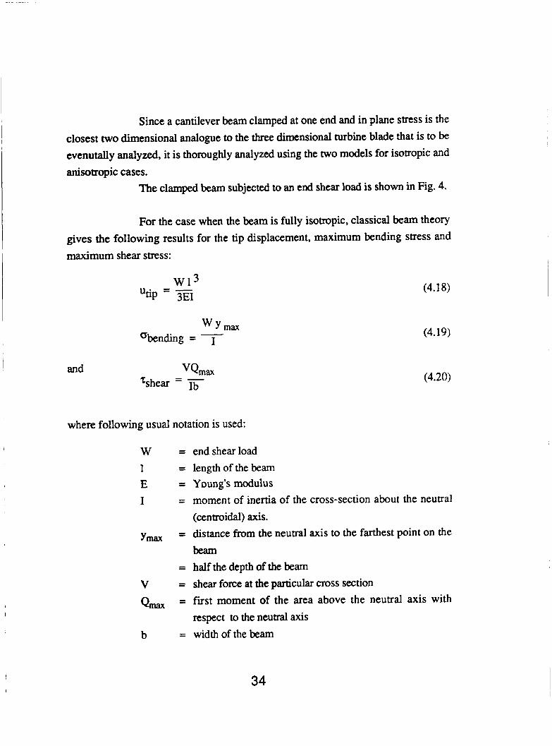
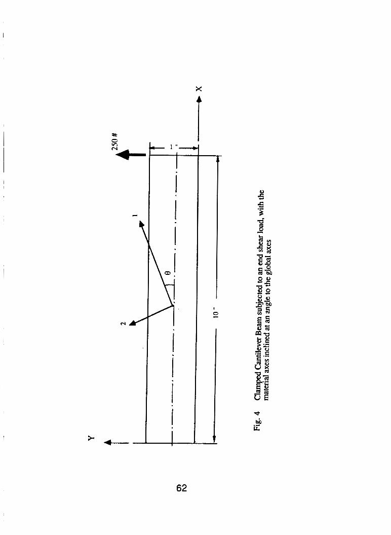
Since a cantilever beam clamped at one end and in plane stress is the closest two dimensional analogue to the three dimensional turbine blade that is to be evenutally analyzed, it is thoroughly analyzed using the two models for isotropic and anisotropic cases.
The clamped beam subjected to an end shear load is shown in Fig. 4.
For the case when the beam is fully isotropic, classical beam theory gives the following results for the tip displacement, maximum bending stress and maximum shear stress:
and
where following usual notation is used:
W 1 E I
V Qmax
b
(4.18)
(4.19)
(4.20)
= end shear load = length of the beam = Young's modulus = moment of inertia of the cross-section about the neutral
(centroidal) axis.
= distance from the neutral axis to the farthest point on the beam
= half the depth of the beam = shear force at the particular cross section = first moment of the area above the neutral axis with
respect to the neutral axis = width of the beam
34
In the case at hand,
W = 2501b. ;
For a rectangular cross section, I = 1/12 bh3 ; b = 1"
= 10" ; h = 1"; E = 3 x lo7 lb./in.2
utip = 0.03333"
%ending max. = 15000 1b./in.2
'shear max. = 375 lb./in.2
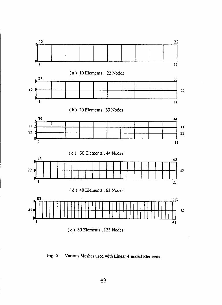
Linear Element Results Using the displacement and the hybrid-stress models, five different
cases were run for an isotropic beam, with the number of linear four-noded elements varying from 10 to 80. The various meshes used in the analysis are shown in Fig. 5.
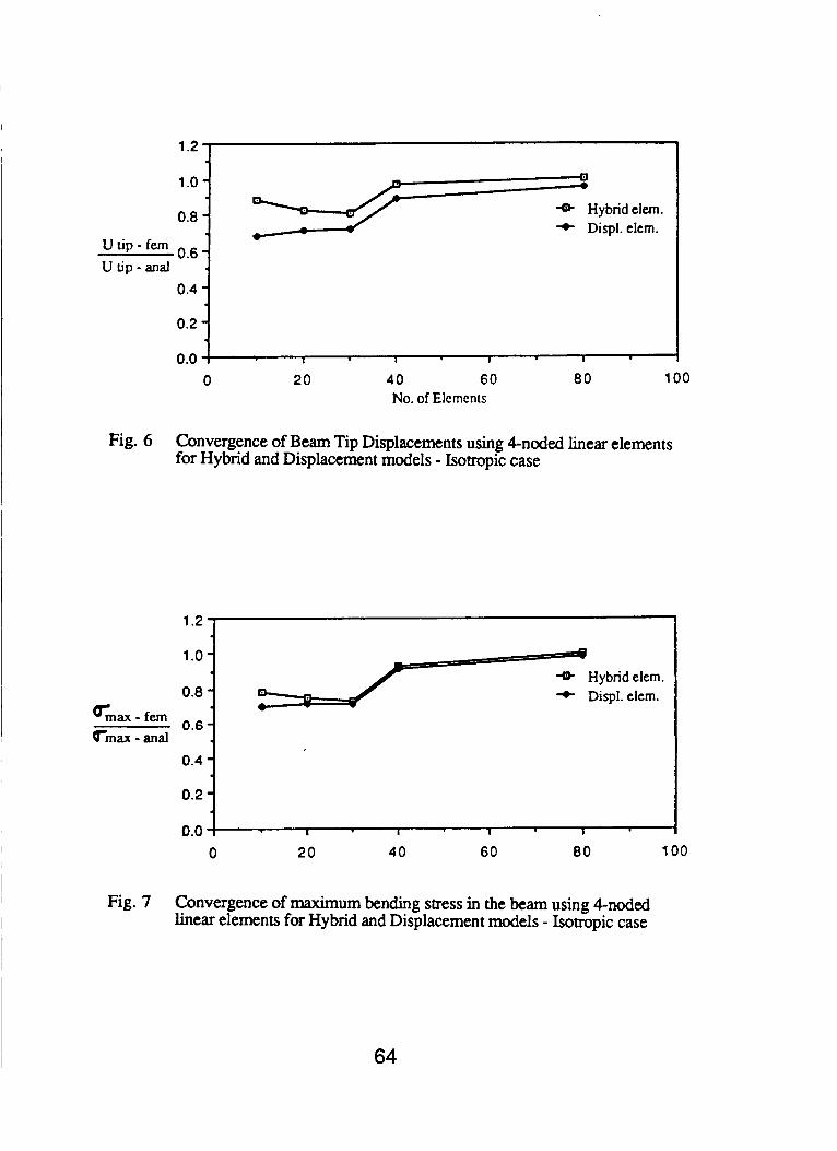
For comparison with analytically obtained results, the normalized tip displacement (Uhybrid/uana].) and the normalized maximum bending stress (q,ybfi&md.) are plotted against the number of elements, and are shown in Fig. 6 and Fig. 7.
It is seen that even for the isotropic case, the hybrid model converges to the analytical solution faster than the assumed displacement model, for identical finite element meshes. Both displacements and stresses obtained using the
hybrid-stress model are consistently better than those obtained using the assumed displacement model.
For the anisotropic case, the material model chosen is that of cubic syngony to simulate the single crystal turbine blade made of the nickel alloy.
From the experimental data supplied, the following material properties were obtained using the materials subroutine described in the previous section discussing Elastic Constants from Experimental Data:
35
E, = 1.9716 x 1071b./in2
4 = 1.9716 x lo7 lb./in2 [neglecting the small difference from E, due to possible errors in measurement].
vi2 = 0.2875 G12 = 5.4758 x lo6 lb./in.2
Using these material properties, the same problem, viz., an end-loaded cantilever, is solved using hybrid and displacement methods.
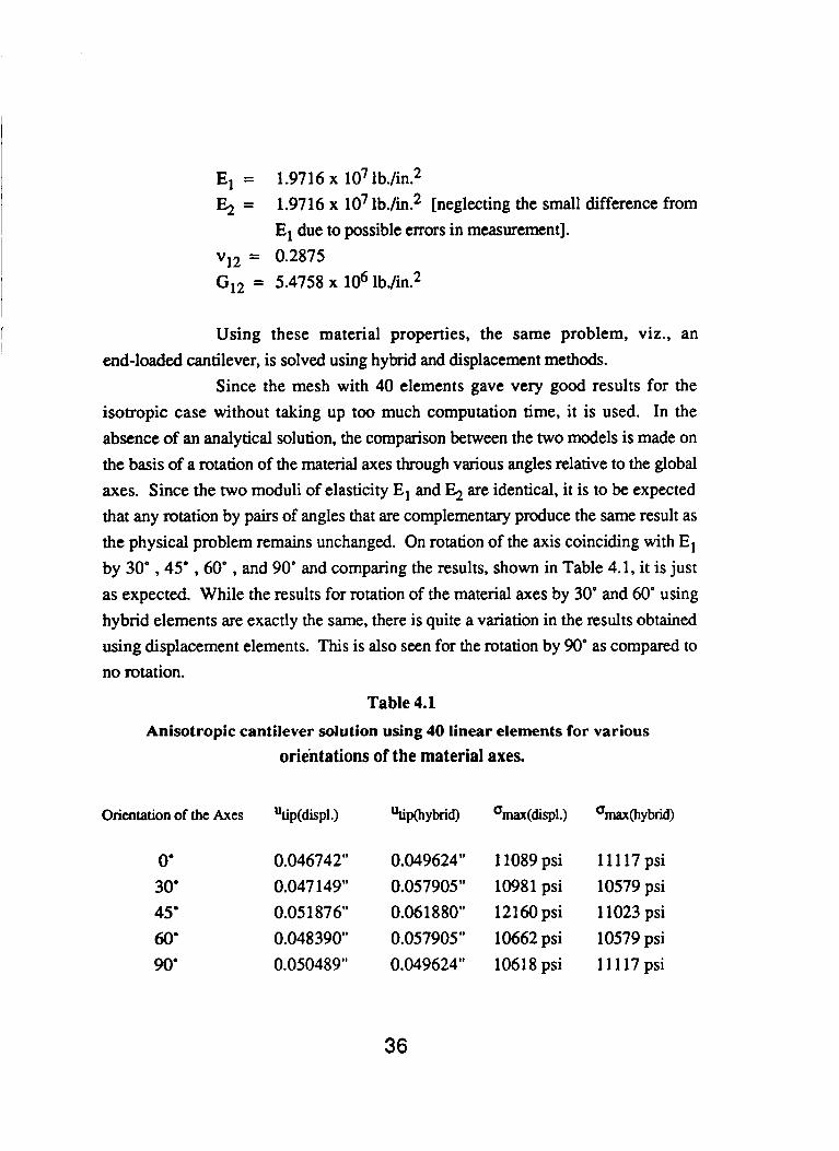
Since the mesh with 40 elements gave very good results for the isotropic case without taking up too much computation time, it is used. In the absence of an analytical solution, the comparison between the two models is made on the basis of a rotation of the material axes through various angles relative to the global axes. Since the two moduli of elasticity E, and 4 are identical, it is to be expected that any rotation by pairs of angles that are complementary produce the same result as the physical problem remains unchanged. On rotation of the axis coinciding with E, by 30" ,45' ,60" , and 90' and comparing the results, shown in Table 4.1, it is just as expected. While the results for rotation of the material axes by 30" and 60" using hybrid elements are exactly the same, there is quite a variation in the results obtained using displacement elements. This is also seen for the rotation by 90' as compared to no rotation.
Table 4.1 Anisotropic cantilever solution using 40 linear elements for various
orientations of the material axes.
Orientation of the Axes Qp(disp1.) %pol ybrid)
0' 0.046742" 0.049624" 30' 0.047 149" 0.057905 I' 45' 0.05 1876" 0.061880" 60' 0.048390" 0.057905 'I 90' 0.050489" 0.049624"
11089 psi 11 117 psi 10981 psi 10579 psi 12160 psi 11023 psi 10662 psi 10579 psi 1061 8 psi 11 117 psi
36
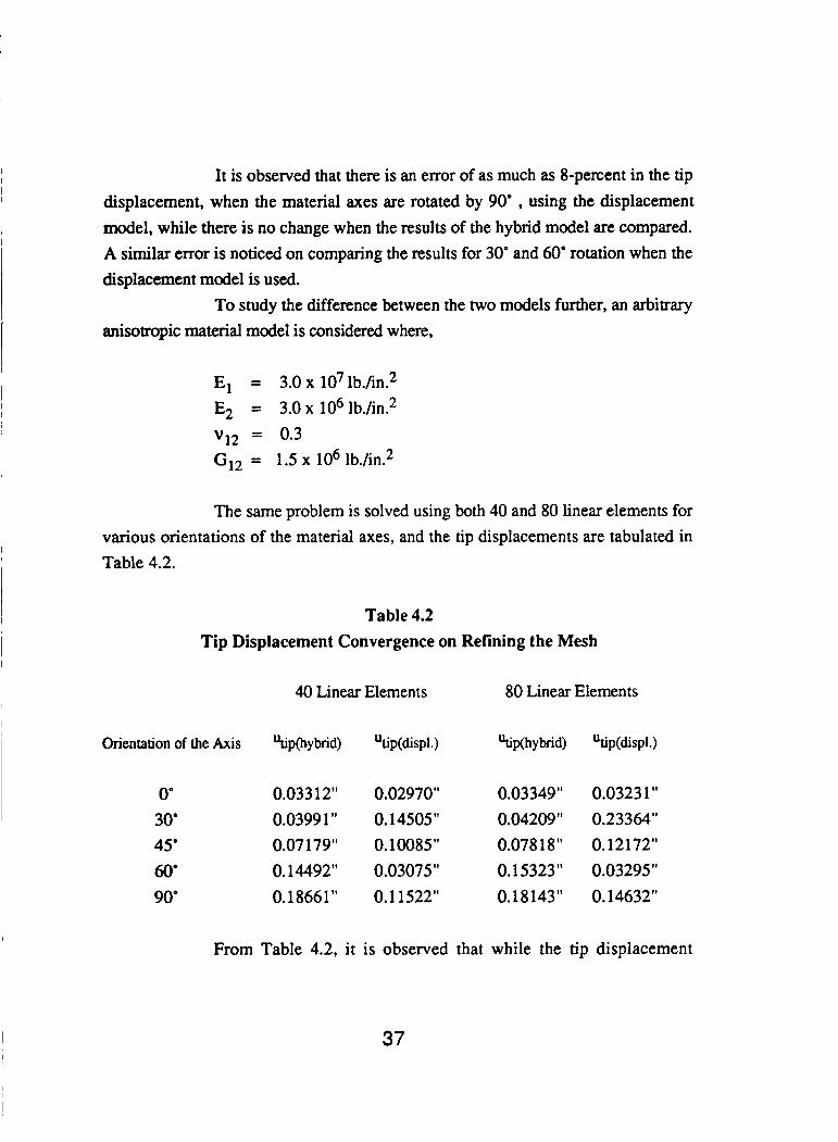
It is observed that there is an error of as much as 8-percent in the tip displacement, when the material axes are rotated by 90' , using the displacement model, while there is no change when the results of the hybrid model are compared. A similar error is noticed on comparing the results for 30' and 60' rotation when the displacement model is used.
To study the difference between the two models further, an arbitrary anisotropic material model is considered where,
E, = 3.0 x lo7 Ib./in., E2 = 3.0 x lo6 Ib./in.2
G,, = 1.5 x lo6 lb./in.2 vi2 = 0.3
The same problem is solved using both 40 and 80 linear elements for various orientations of the material axes, and the tip displacements are tabulated in Table 4.2.
Table 4.2 Tip Displacement Convergence on Refining the Mesh
40 Linear Elements 80 Linear Elements
Orientation of the Axis
0' 30' 45'
60' 90'
%p(hybrid) 'tip(disp1.) %p(hybrid) 'tip(disp1.)
0.033 12" 0.02970" 0.03349" 0.0323 1" 0.03991" 0.14505" 0.04209" 0.23364" 0.07179" 0.10085" 0.078 18" 0.12172" 0.14492" 0.03075" 0.15323" 0.03295" 0.1866 1" 0.1 1522" 0.18143" 0.14632"
From Table 4.2, it is observed that while the tip displacement
37
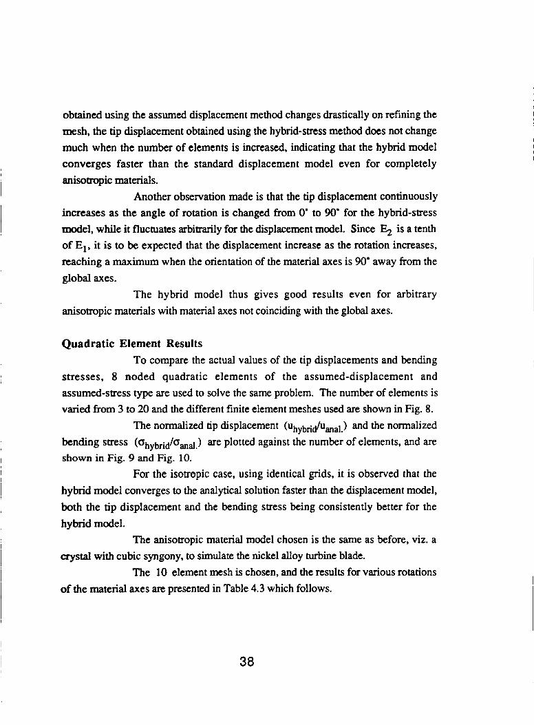
obtained using the assumed displacement method changes drastically on refining the mesh, the tip displacement obtained using the hybrid-stress method does not change much when the number of elements is increased, indicating that the hybrid model converges faster than the standard displacement model even for completely anisotropic materials.
Another observation made is that the tip displacement continuously increases as the angle of rotation is changed from 0' to 90' for the hybrid-stress model, while it fluctuates arbitrarily for the displacement model. Since is a tenth of E,, it is to be expected that the displacement increase as the rotation increases, reaching a maximum when the orientation of the material axes is 90' away from the global axes.
The hybrid model thus gives good results even for arbitrary anisotropic materials with material axes not coinciding with the global axes.
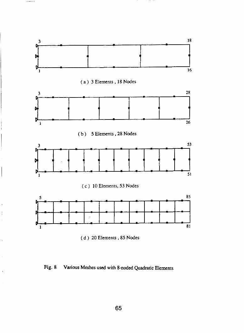
Quadratic Element Results To compare the actual values of the tip displacements and bending
stresses, 8 noded quadratic elements of the assumed-displacement and assumed-stress type are used to solve the same problem. The number of elements is varied from 3 to 20 and the different finite element meshes used are shown in Fig. 8.
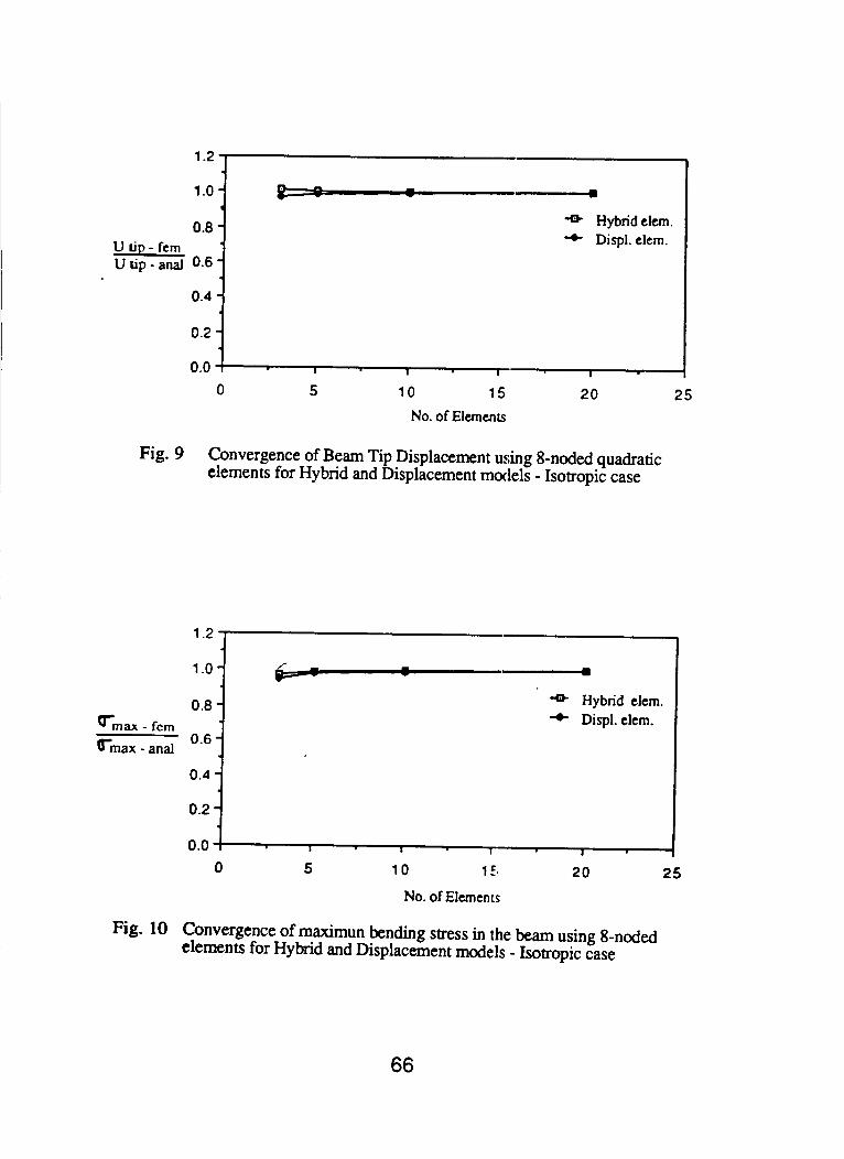
The normalized tip displacement (q,ybfi&anal.) and the normalized bending stress (ohybri&r,,.) are plotted against the number of elements, and are
For the isotropic case, using identical grids, it is observed that the hybrid model converges to the analytical solution faster than the displacement model, both the tip displacement and the bending stress being consistently better for the hybrid model.
The anisotropic material model chosen is the same as before, viz. a crystal with cubic syngony, to simulate the nickel alloy turbine blade.
The 10 element mesh is chosen, and the results for various rotations of the material axes are presented in Table 4.3 which follows.
shown in Fig. 9 and Fig. 10.
38
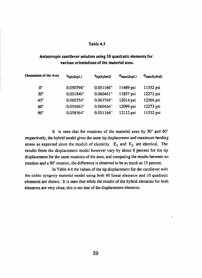
Table 4.3
Anisotropic cantilever solution using 10 quadratic elements for various orientations of the material axes.
Orientation of the Axes
0' 30' 45' 60' 90'
utiP(disp1.) %p(hybrid) %ax(dspl.) %ax(hybrid)
0.050798" 0.05 1 166" 1 1489 psi 1 1532 psi 0.05 1840" 0.060461" 11857 psi 12272 psi 0.060356" 0.063769" 12014 psi 12566 psi 0.054663" 0.060464" 12099 psi 12273 psi 0.05 8 364" 0.051 166" 121 12 psi 11532 psi
It is seen that for rotations of the material axes by 30' and 60" respectively, the hybrid model gives the same tip displacement and maximum bending stress as expected since the moduli of elasticity E, and E, are identical. The results from the displacement model however vary by about 6 percent for the tip displacement for the same rotations of the axes, and comparing the results between no rotation and a 90" rotation, the difference is observed to be as much as 15 percent.
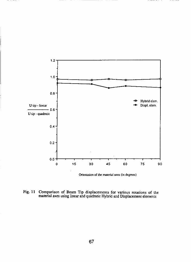
In Table 4.4 the values of the tip displacement for the cantilever with the cubic syngony material model using both 40 linear elements and 10 quadratic elements are shown. It is seen that while the results of the hybrid elements for both elements are very close, this is not true of the displacement elements.
39
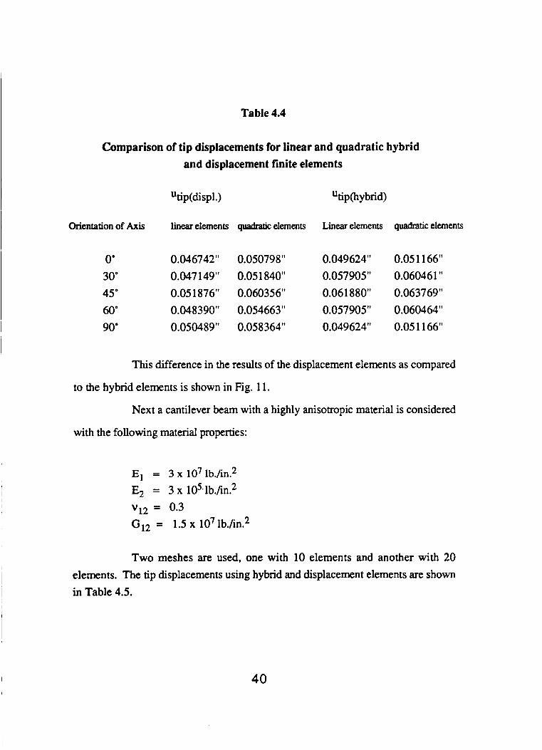
Table 4.4
Comparison of tip displacements for linear and quadratic hybrid and displacement finite elements
Utip(disp1.) tipmybrid)
Orientation of Axis linear elements quadratic elements Linear elements quadratic elements
0' 0.046742" 0.050798" 0.049624" 0.05 1 166" 30' 0.047 149" 0.05 1840" 0.057905" 0.060461 45' 0.05 1876" 0.060356" 0.061 880" 0.063769" 60' 0.048390" 0.054663" 0.057905" 0.060464" 90" 0.050489" 0.058364" 0.049624" 0.05 1 166"
This difference in the results of the displacement elements as compared
to the hybrid elements is shown in Fig. 11.
Next a cantilever beam with a highly anisotropic material is considered
with the following material properties:
E, = 3 x lo7 Ib./h2 E, = 3 x 1O5,lb./in2
GI, = 1.5 x 1071b./in.* vi2 = 0.3
Two meshes are used, one with 10 elements and another with 20 elements. The tip displacements using hybrid and displacement elements are shown in Table 4.5.
40
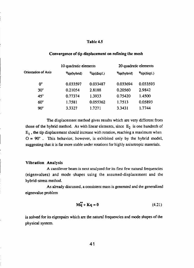
Table 4.5
Convergence of tip displacement on refining the mesh
10 quadratic elements 20 quadratic elements
Orientation of Axis %p(hybrid) "tip(disp1.) "upolybrid) utip(displ.)
0' 0.033597 0.033487 0.033694 0.033593 30' 0.21054 2.8188 0.20560 2.9842 45' 0.77374 1.3933 0.75420 1.4500 60' 1.7581 0.05 5 3 62 1.7513 0.05893 90' 3.3327 1.727 1 3.3431 1.7744
The displacement method gives results which are very different from those of the hybrid method. As with linear elements, since is one hundreth of E, , the tip displacement should increase with rotation, reaching a maximum when 0 = 90' . This behavior, however, is exhibited only by the hybrid model, suggesting that it is far more stable under rotations for highly anisotropic materials.
Vibration Analysis A cantilever beam is next analyzed for its first few natural frequencies
(eigenvalues) and mode , shapes using the assumed-displacement and the hybrid-stress method.
As already discussed, a consistent mass is generated and the generalized eigenvalue problem
Mt+ Kq = 0 (4.21)
is solved for its eigenpairs which are the natural frequencies and mode shapes of the physical system.
41
Since the size of the matrices is not very large, a solver from IMSL that determines all the eigenvalues and eigenvectors is used instead of the sub-space iteration scheme suggested by Bathe [13].
For Bernoulli-Euler beams made of isotropic materials, neglecting the effect of shear deformation and rotatory inertia as we will consider only the first two modes where the correction introduced as a result of these effects is small, the equation of motion for transverse vibration is
where
d2 d% d%
dx2 dx2 dt2 - @I-) + P A - = 0
v = v(x,t) is the transverse displacement,
(4.22)
A = area of cross section of the beam
x = axial distance from the point of support
p = mass density of the material
I = centroidal moment of inertia of the cross-section
The boundary conditions for the cantilever are:
v = O and
dv - = o dx
At the futed end;
2 d v - = O and dx2
At the free end; d3v - = o d x 3 (4.23)
Substituting the boundary conditions into general solution, we get three homogeneous linear algebraic equations which yield a non-trivial solution only if the
42
determinant of the coefficients vanishes, i.e.
1 +CoshL CoshhL + 1 = 0 (4.24)
which is the characteristic equation whose roots are the eigenvalues h, times length L. A numerical solution exists for the above equation, determined by Craig and Chang [ 141. The first few values are
hlL = 1.8751
&L = 4.6941
and the natural frequencies for the cantilever are given by
so that 3.516 E1 ”
01 = -( -) L2 PA
and
(4.25)
Substituting the numerical values for the given problem, we get
01 = 17.58 Hz. , 02 = 110.15 Hz.
The mode shapes are given by
V,(x) = Cosh (Q) - Cos(+) - k,[Sinh(+) - Sin (+)I (4.26)
where
43
(4.27)
as in Craig [20].
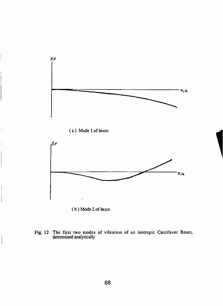
Fig. 12. The first two mode shapes for a cantilever in free vibration are shown in
Linear Element Results The meshes that were used for the static problem axe used here, with the
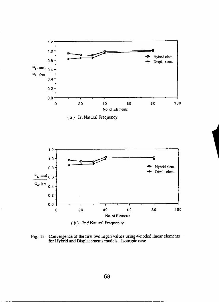
number of elements varying from 10 to 80. The normalized natural frequencies (a1 anal. /~l f.e. and 02 anal./% f.e.)
are plotted against the number of elements, and are shown in Fig. 13 . For the isotropic case, the hybrid model converges to the analytical
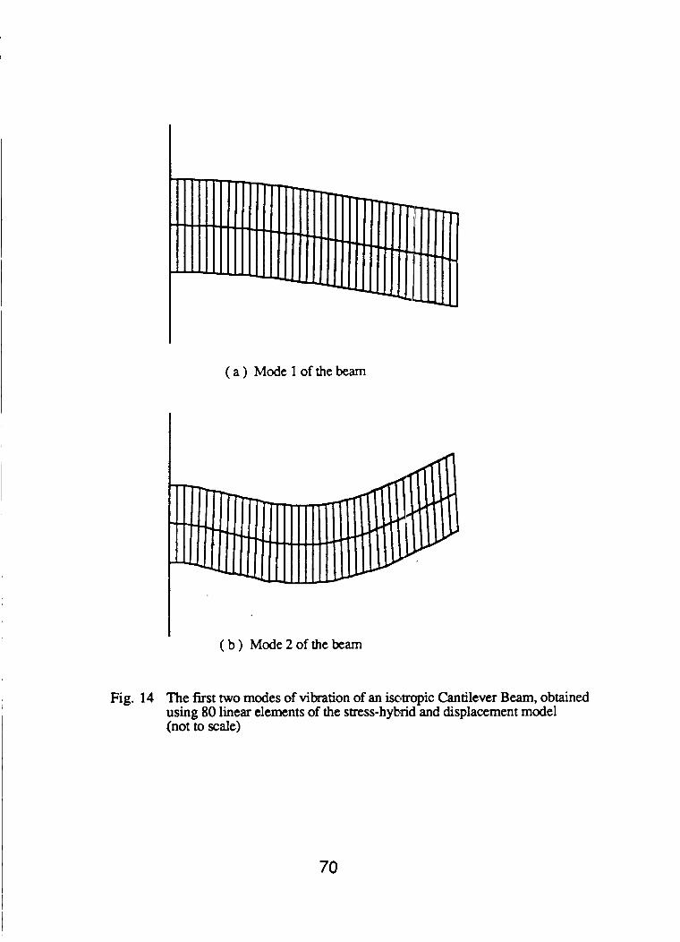
solution faster than the assumed displacement model. The mode shapes however do not seem to vary much, as seen in Fig. 14 (for the mesh with 80 elements).
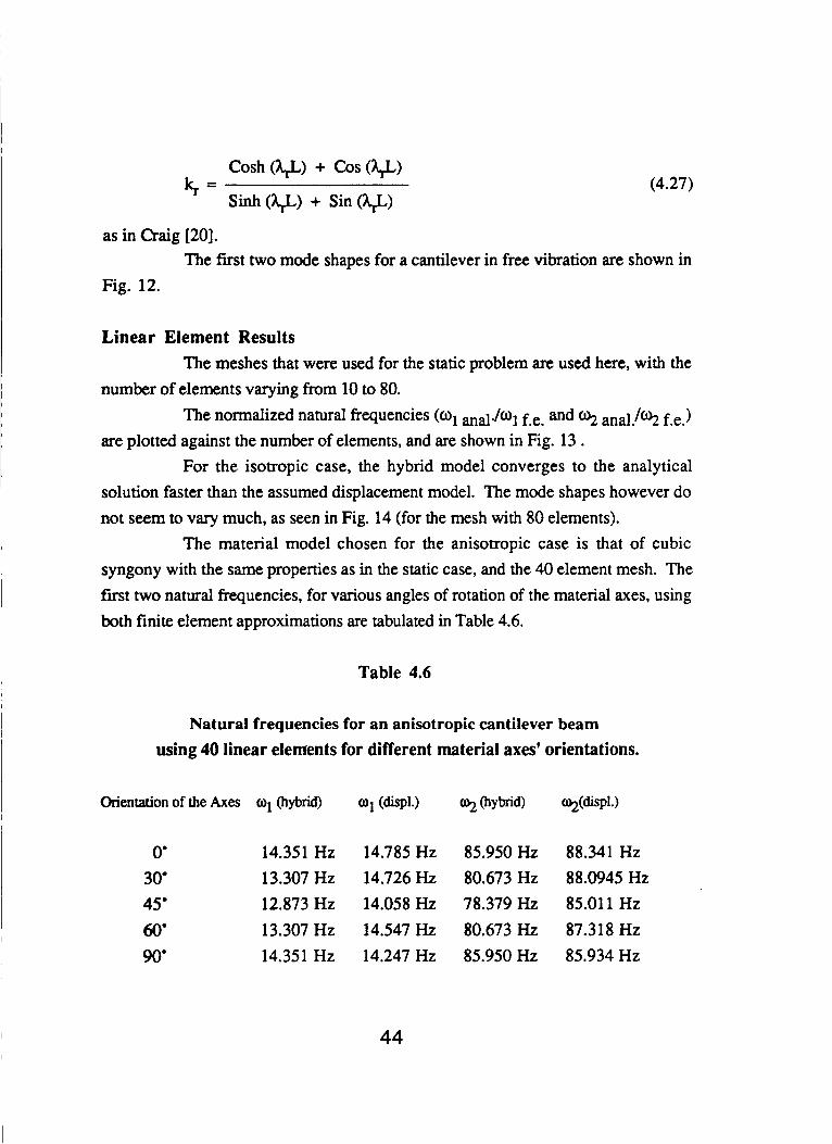
The material model chosen for the anisotropic case is that of cubic syngony with the same properties as in the static case, and the 40 element mesh. The first two natural frequencies, for various angles of rotation of the material axes, using both finite element approximations are tabulated in Table 4.6.
Table 4.6
Natural frequencies for an anisotropic cantilever beam using 40 linear elements for different material axes' orientations.
Orientation of the Axes o1 (hybrid)
0' 14.351 Hz 30' 13.307 Hz 45' 12.873 Hz 60' 13.307 Hz 90' 14.351 Hz
14.785 Hz 85.950 Hz 14.726 Hz 80.673 Hz 14.058 Hz 78.379 Hz 14.547 Hz 80.673 Hz 14.247 Hz 85.950 Hz
y p s p l . )
88.341 Hz 88.0945 Hz 85.011 Hz 87.318 Hz 85.934 Hz
44
From the above table it is observed that the hybrid model gives identical results for a rotation of 90' and no rotation of the material axes, 30' and 60' of the axes. The displacement method however gives results that vary, even though the moduli E1 and E2 are q u a l .
The first two mode shapes for the anisotropic cantilever, obtained using both the models do not vary much as shown in Fig. 15 (even for the case when the the difference between the eigen values is a maximum, viz., for 8 = 45O).
Quadratic Element Results The natural frequencies and mode shapes of the isotropic and anisotropic
cantilever beams are now calculated using an 8-node43 finite element mesh with the number of elements varying from 3 to 20. The meshes used are the same as for the static case and are shown in Fig. 8.
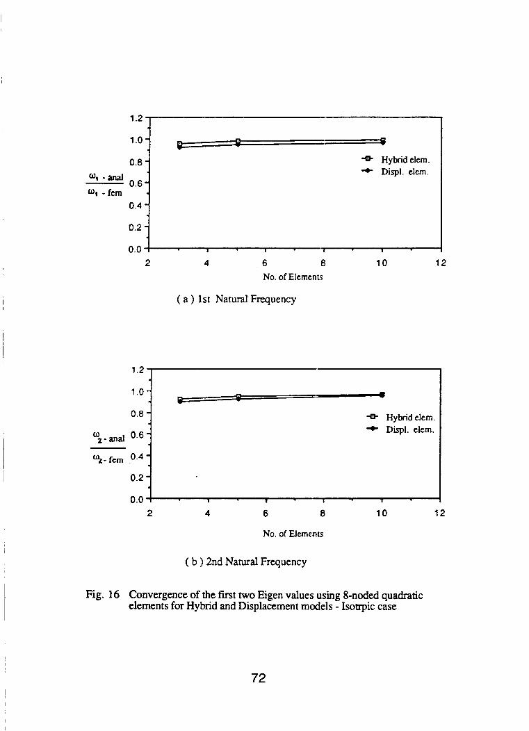
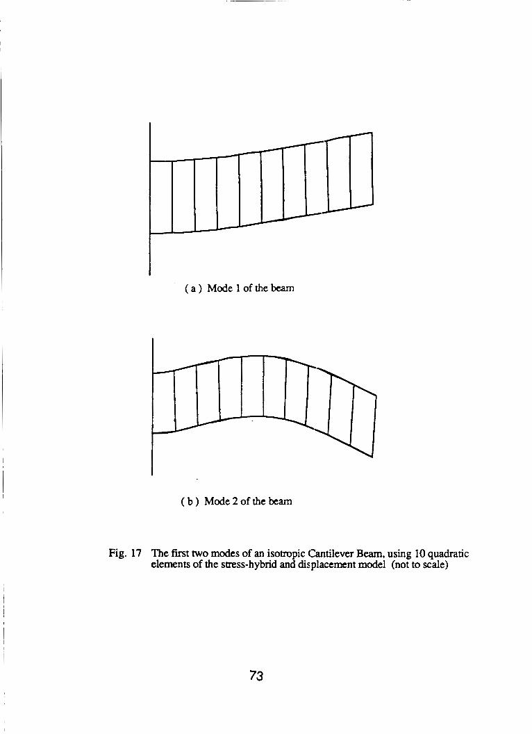
The normalized natural frequencies (01 anal . /~l f.e. and 02 f.e.) are plotted against the number of elements, and are shown in Fig. 16. Again, it is observed that the hybrid model converges to the analytical solution faster than the assumed-displacement method. The mode shapes however are very similar in both models, except for the maximum "amplitude" (when 10 quadratic elements are used) as shown in Fig. 17.
The first two natural frequencies for various angles of rotation of the material axes, in an anisotropic cantilever beam, using both the displacement and hybrid approximations are tabulated in Table 4.7. The material properties and the
material model assumed are the same as for the static anisotropic case, viz. 3 independent constants in a crystal with cubic syngony, where
E, = E, = 1.9716~ 1071b./in.2
~ 1 2 = 0.2875
G12 = 5.4758 x 1O61b./in2
45
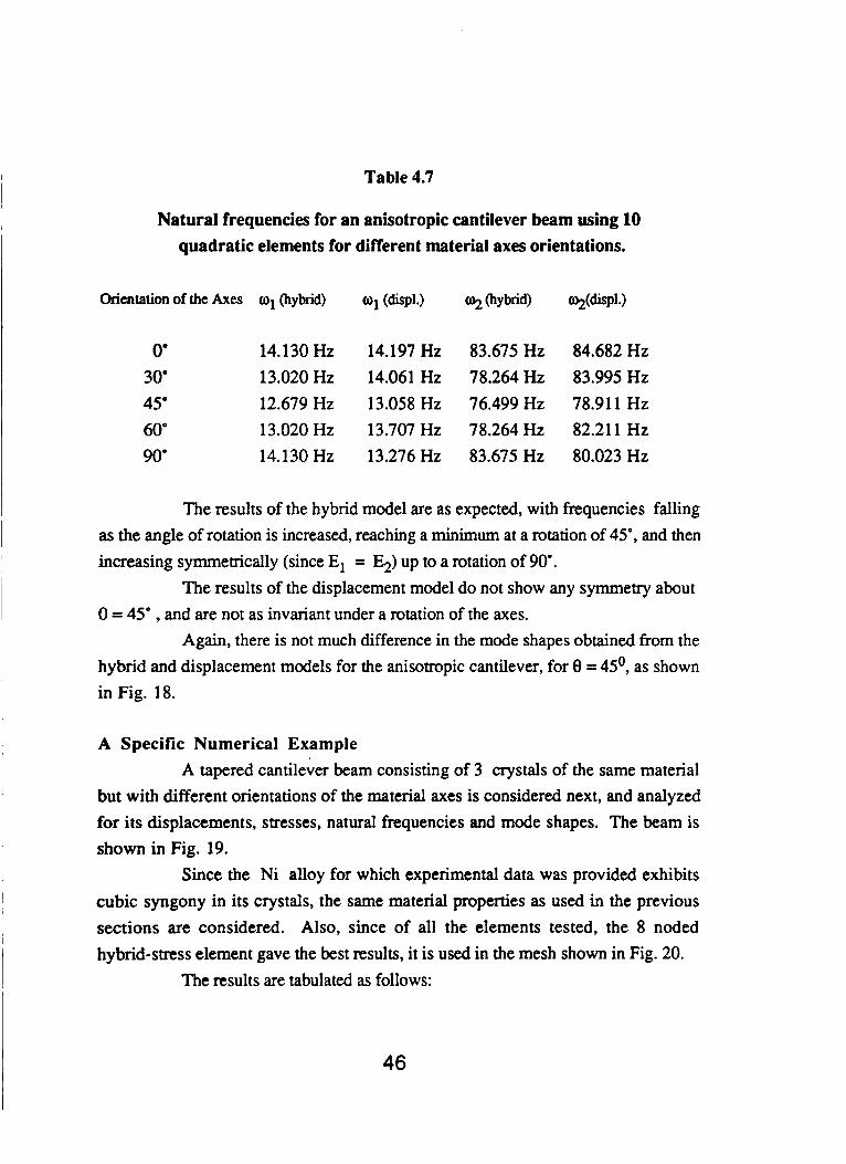
Table 4.7
Natural frequencies for an anisotropic cantilever beam using 10 quadratic elements for different material axes orientations.
Orientation of the Axes o1 (hybrid)
0' 14.130 Hz 30' 13.020 Hz 45' 12.679 Hz 60' 13.020 Hz 90' 14.130 Hz
0 1 (diSpl.1
14.197 Hz 14.061 Hz 13.058 Hz 13.707 Hz 13.276 Hz
02 (hybrid)
83.675 Hz 78.264 Hz 76.499 Hz 78.264 Hz 83.675 Hz
02(diSpl.)
84.682 Hz 83.995 Hz 78.911 Hz 82.211 Hz 80.023 Hz
The results of the hybrid model are as expected, with frequencies falling as the angle of rotation is increased, reaching a minimum at a rotation of 45', and then increasing symmetrically (since E, = E2) up to a rotation of 90".
The results of the displacement model do not show any symmetry about 0 = 45' , and are not as invariant under a rotation of the axes.
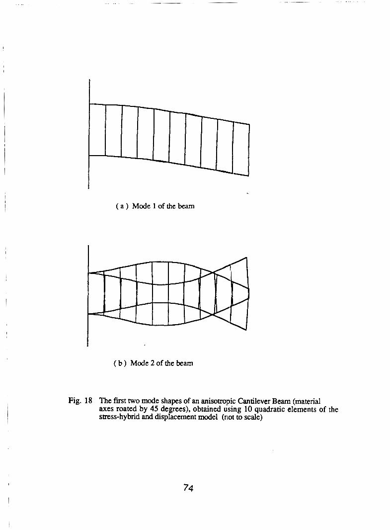
Again, there is not much difference in the mode shapes obtained from the hybrid and displacement models for the anisotropic cantilever, for 0 = 45O, as shown in Fig. 18.
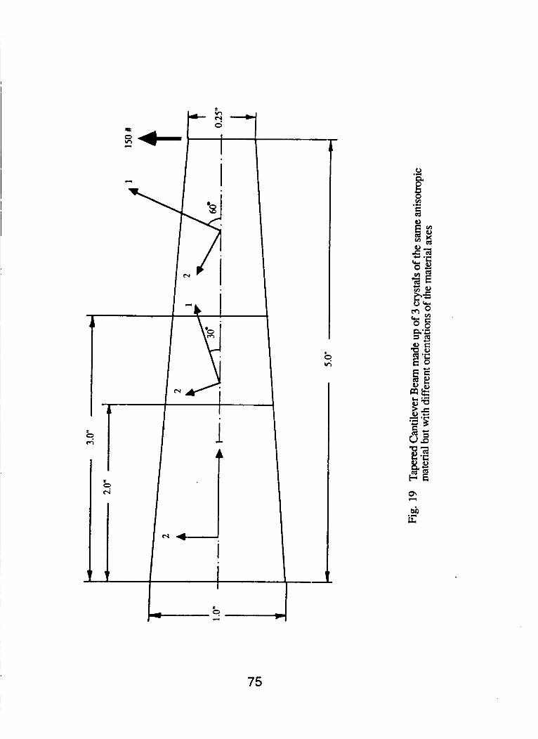
A Specific Numerical Example A tapered cantilever beam consisting of 3 crystals of the same material
but with different orientations of the material axes is considered next, and analyzed for its displacements, stresses, natural frequencies and mode shapes. The beam is shown in Fig. 19.
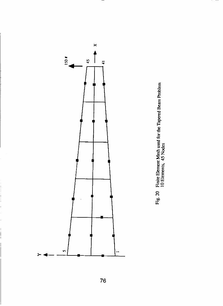
Since the Ni alloy for which experimental data was provided exhibits cubic syngony in its crystals, the same material properties as used in the previous sections are considered. Also, since of all the elements tested, the 8 noded hybrid-stress element gave the best xesults, it is used in the mesh shown in Fig. 20.
The results are tabulated as follows:
46
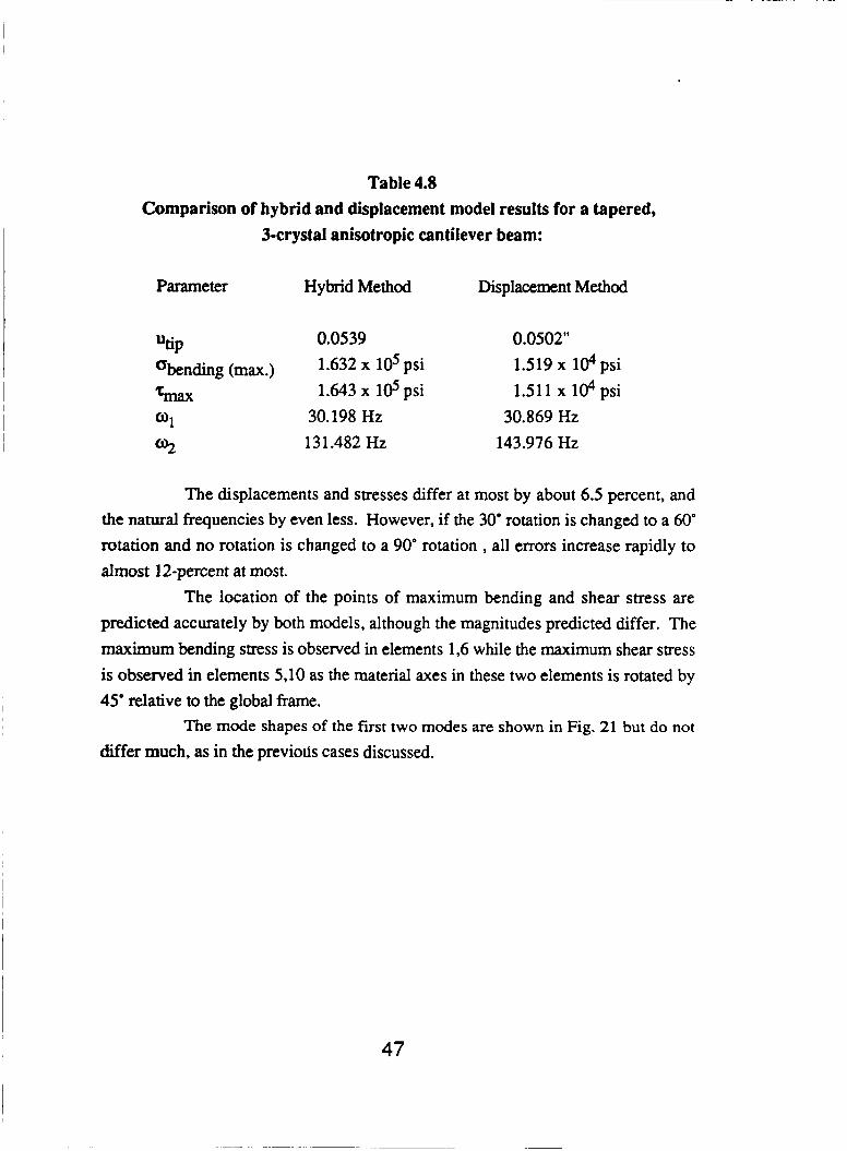
Table 4.8 Comparison of hybrid and displacement model results for a tapered,
3-crystal anisotropic cantilever beam:
Parameter Hybrid Method Displacement Method
"tip 0.0539 0.0502" %ending (max.) 1.632 x lo5 psi 1.519 x l@psi
%lax 1.643 x 10⁵ psi 1.511 x 10⁴ psi
0 1 30.198 Hz 30.869 Hz
w2 13 1.482 Hz 143.976 Hz
The displacements and stresses differ at most by about 6.5 percent, and the natural frequencies by even less. However, if the 30' rotation is changed to a 60' rotation and no rotation is changed to a 90' rotation , all errors increase rapidly to almost 12-percent at most.
The location of the points of maximum bending and shear stress are predicted accurately by both models, although the magnitudes predicted differ. The maximum bending stress is observed in elements 1,6 while the maximum shear stress is observed in elements 5,lO as the material axes in these two elements is rotated by 45' relative to the global frame.
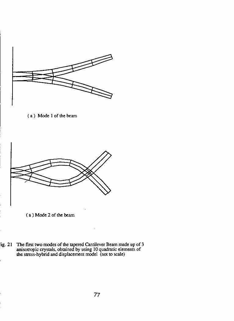
The mode shapes of the first two modes are shown in Fig, 21 but do not
differ much, as in the previods cases discussed.
47
SUMMARY AND CONCLUSIONS
In this work, a hybrid-stress finite element method is developed for equilibrium and vibration analysis of problems in two-dimensional anisotropic elasticity.
A number of sample problems are solved using the hybrid-stress method and the standard displacement method and the results are compared. Emphasis is placed on a cantilever beam loaded in end shear because of its similarity to a turbine blade.
It is observed that even for the isotropic case, the hybrid-stress model gives more accurate displacements, stresses and natural frequencies as compared to the results of the displacement method, although the variation between the two is not large.
For anisotropic materials, especially when the material axes are rotated relative to the global axes, the hybrid-stress model is observed to be stable and invariant, while the displacement model shows some variation for pairs of rotations that are complementary when the two Young's moduli E, and E, are equal.
comparisons are made by increasing the number of elements and checking for convergence. The hybrid model behaves well even if the number of elements used is not too large, although if the degree of anisotropy is very high, e.g. E1E2 = 104, both models do not seem to converge rapidly.
Work is now in progress to extend the finite element code to include three
dimensional problems. The'stress shape functions for 8-noded linear bricks and 20-noded quadratic brick elements as proposed by Rubinstein, Punch and Atluri [6] will be implemented in the hybrid-stress finite element code and compared with the 8-noded and 20-noded brick elements using a displacement approximation.
Instead of using group theoretical methods to determine stable, invariant stress fields, complete stress polynomials may be chosen and the number of stress parameters reduced by forcing equilibrium and compatibility conditions to be satisfied. Although the algebra involved is tedious and the matrices are slightly stiffer, the element matrices will be very stable under rotation and the results thus
In the absence of analytical solutions for anisotropic cantilever beams,
48
obtained may be compared with those obtained using the group theoretical stress polynomials.
Once a three-dimensional finite element mesh has been generated for the anisotropic crystalline turbine blade, the above scheme may be used to analyze it statically and dynamically for stresses, displacements, natural frequencies and mode shapes.
Another suggested development would be to investigate the use of triangular elements for two-dimensional hybrid-stress finite element analysis, and tetrahedrons for three-dimensional problems.
49
APPENDIX A
C-LCULATION OF THE POLYNOML -L STRESS FUP. CTIONS FOR LINEAR (7 R) AND QUADRATIC (15 R) QUADRILATERAL
ELEMENTS
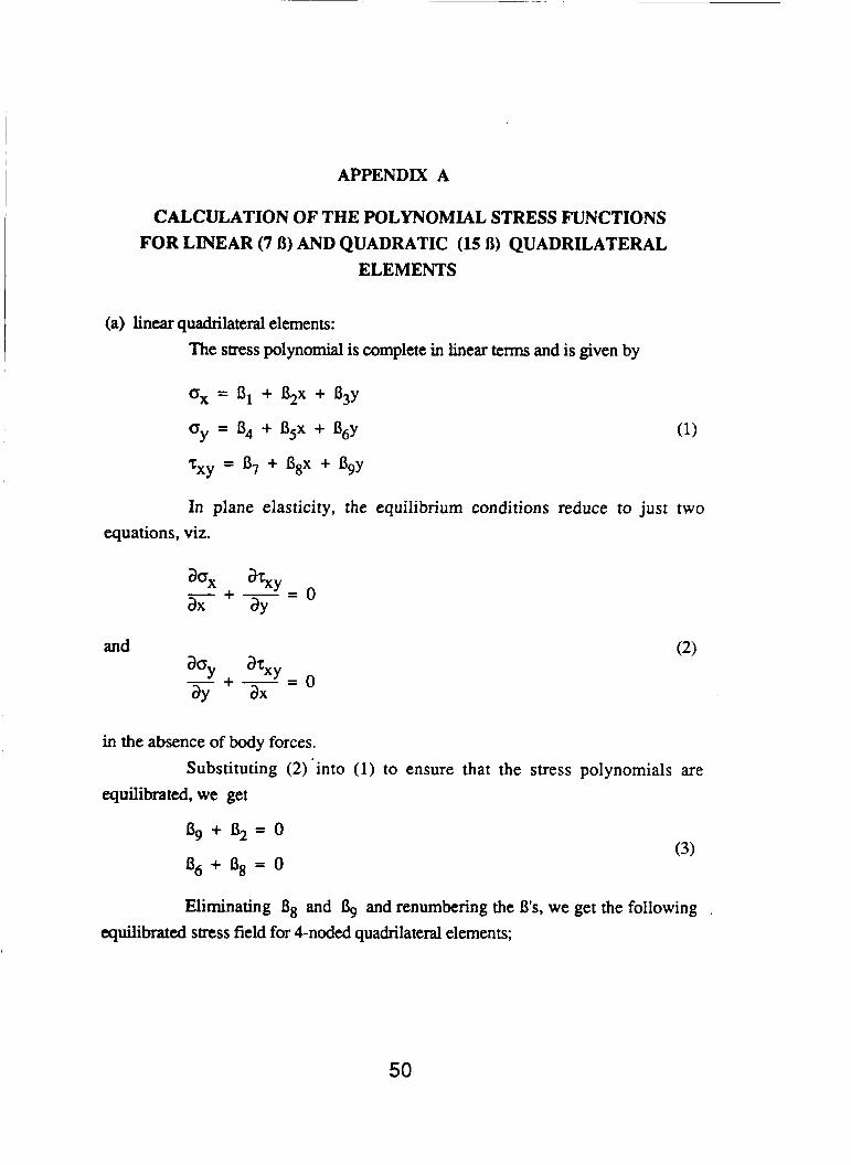
(a) linear quadrilateral elements: The stress polynomial is complete in linear t e rn and is given by
l ox = 13, + B ~ x + B ~ Y
= 13, + 13,x + 13gy =XY
I oy = 84 + B,x + 13,y (1)
In plane elasticity, the equilibrium conditions reduce to just two equations, viz.
and - aoY + - = 0 ay ax
in the absence of body forces.
equilibrated, we get Substituting (2)'into (1) to ensure that the stress polynomials are
Eliminating B8 and 4 and renumbering the B's, we get the following equilibrated stress field for 4-noded quadrilateral elements;
50
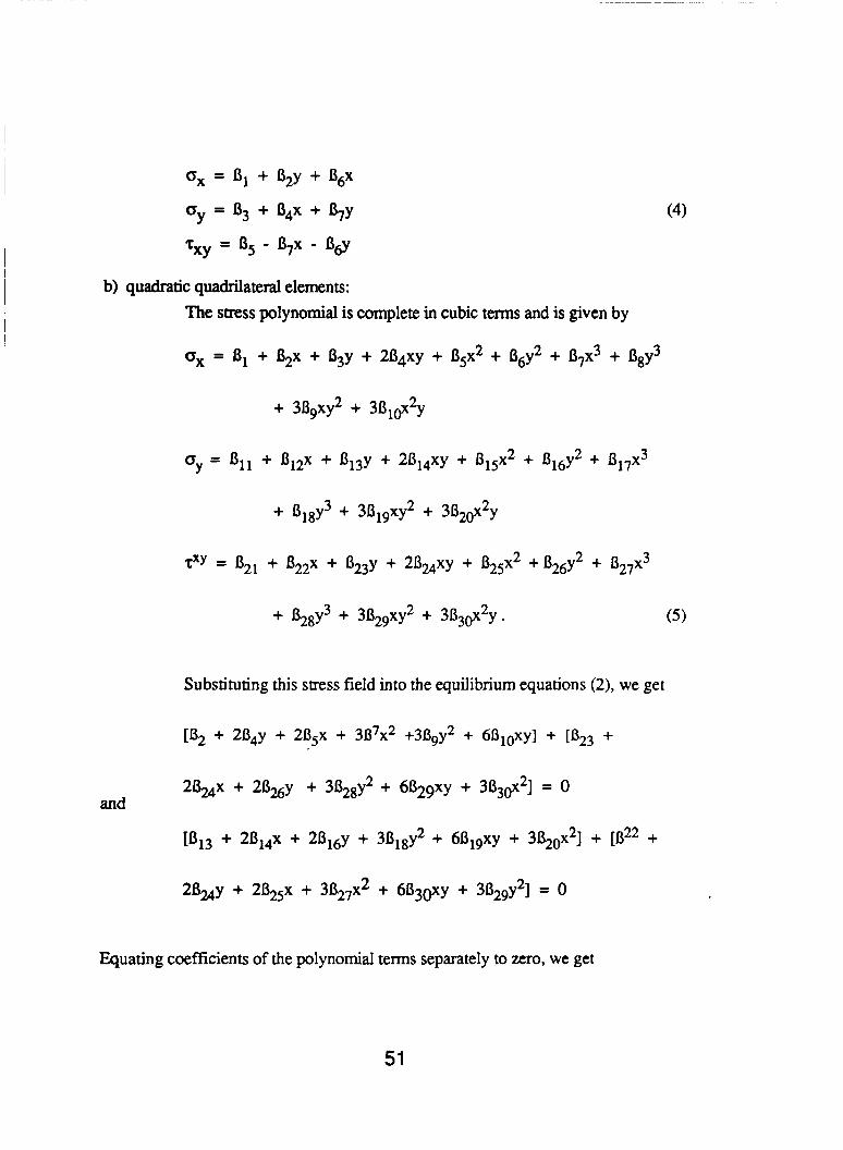
b) quadratic quadrilateral elements: The stress polynomial is complete in cubic terms and is given by
ox = S, + B2x + B3y + 2S4xy + B5x2 + 06y2 + B7x3 + 08y3
Substituting this stress field into the equilibrium equations (2), we get
Equating coefficients of the polynomial terms separately to zero, we get
51
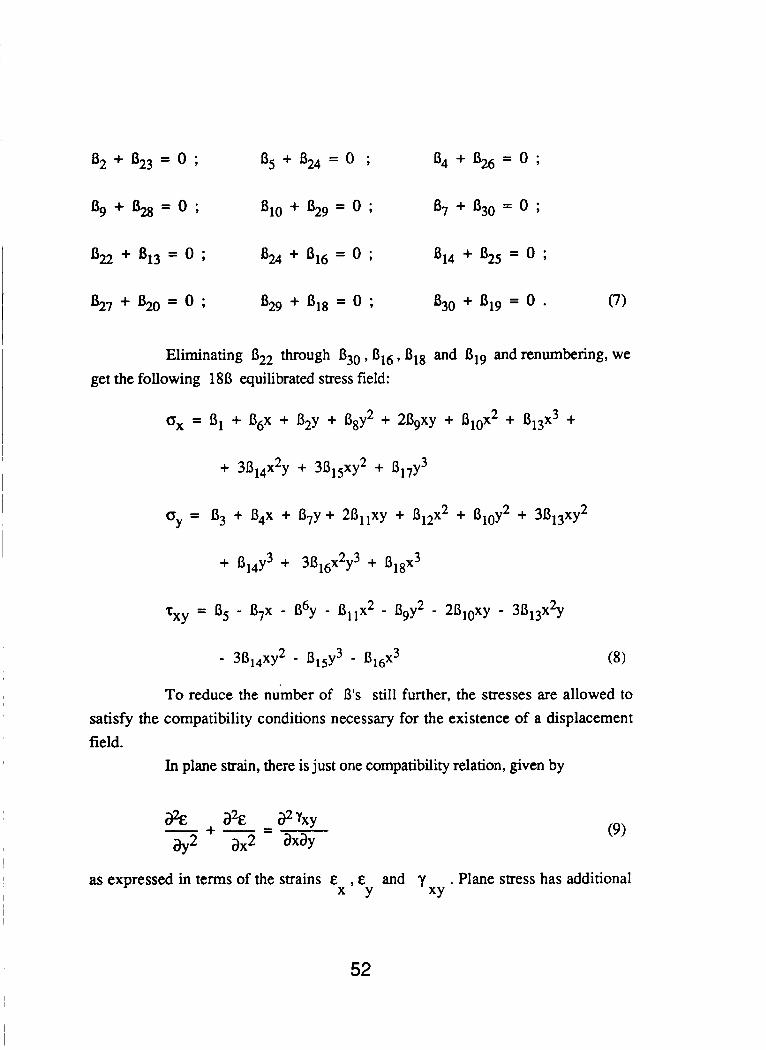
B2 + 823 = 0 ; 135 + B24 = 0 ; 84 + B, = 0 ;
0g+B28=0; 1310 + 829 = 0 ; 0, + B,, = 0 ;
0, + 4 3 = 0 ; B, + B1(j = 0 ; B14 + B25 = 0 ;
Eliminating B2, through 830, B 1 6 , 818 and 819 and renumbering, we get the following 1813 equilibrated stress field:
= 11, + 134x + B7y + 2B,,xy + B,,x2 + B,oY + 3013Xy2 OY
- 3814Xy2 - ~ , , y 3 - (8)
To reduce the number of 13's still further, the stresses are allowed to satisfy the compatibility conditions necessary for the existence of a displacement field.
In plane strain, there is just one compatibility relation, given by
as expressed in terms of the strains E , E and y . Plane stress has additional X Y XY
52
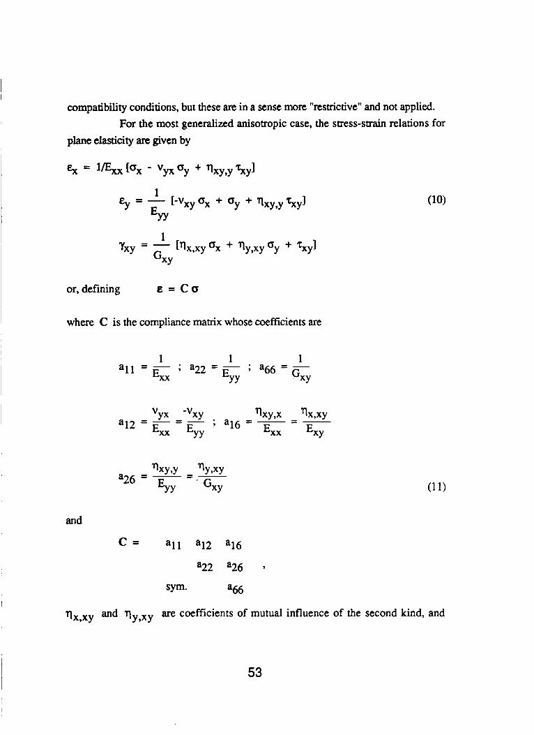
compatibility conditions, but these are in a sense more "restrictive" and not applied.
plane elasticity are given by For the most generalized anisotropic case, the stress-strain relations for
1 [qx,xyox + qy,xy'y + '5xYl Yxy = -
GXY
or, defining e = c o
where C is the compliance matrix whose coefficients are
1 1 1
and
C = al l a12 a16
a22 a26 9
SYm. a66
rlx,xy and qy,xy are coefficients of mutual influence of the second kind, and
53
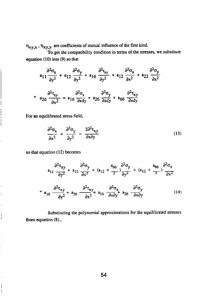
are coefficients of mutual influence of the fmt kind. “Y,X ’ qxy,y To get the compatibility condition in terms of the stresses, we substitute
equation (10) into (9) so that
For an equilibrated stress field,
azox a%, 2a2zxy
ax2 ay2 axay + - = -
so that equation (12) becomes
Substituting the polynomial approximations for the equilibrated stresses from equation (8) ,
54
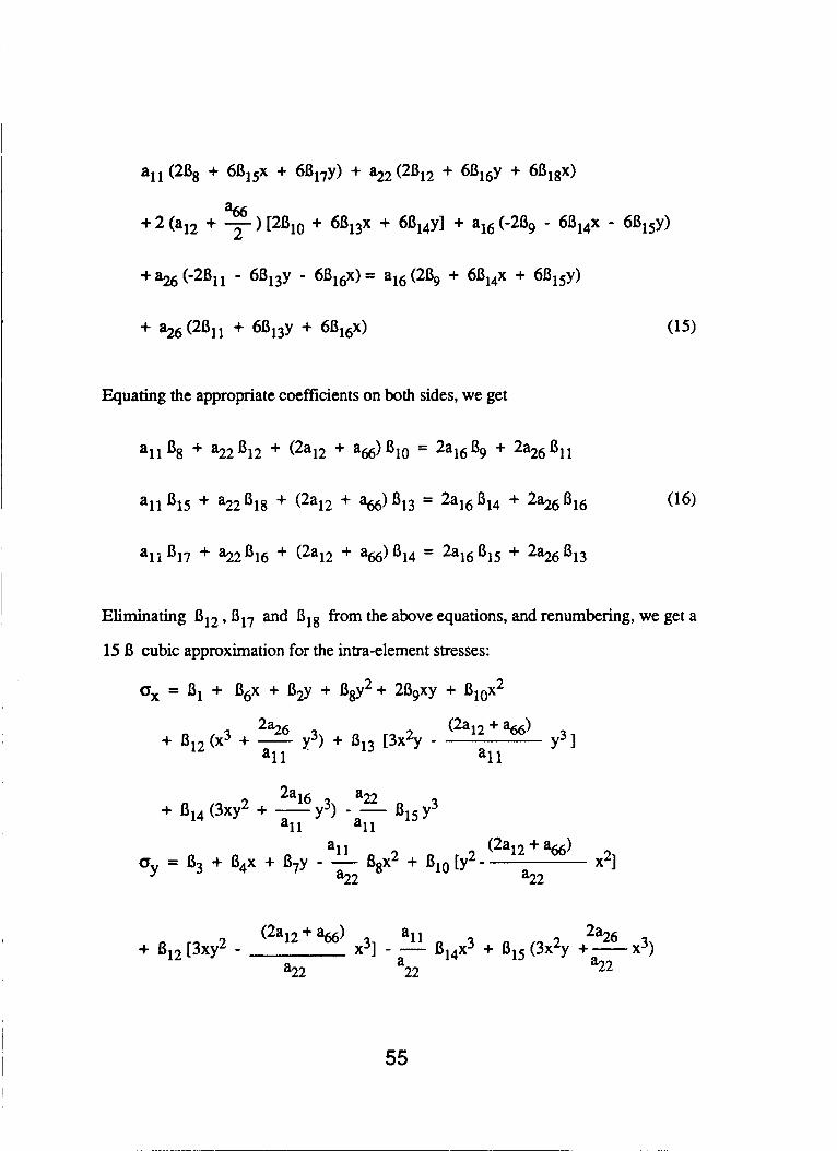
Equating the appropriate coefficients on both sides, we get
Eliminating 13,, ,1317 and '18 from the above equations, and renumbering, we get a
15 13 cubic approximation for the intra-element stresses:
*X = 131 + 136x + 82y + 6gy2+ 2139xy + 810x2
Y3 I + a66) 2%6 3 + B12(x + - Y3) + '13 i3'5
a1 1 a1 1
55

2a16 x3) + 2a16 - BgX2 + 81, (2xy + 2%- x2) a22 a22
+ B13(Y3 + 822
For an isotropic material,
a16 - - a26 = 0 , and 2a12 + a& = 2all
all = a22 ' so that the stress field loses all dependence on the compliance constants and becomes simply
56
REFERENCES
1. pian, T.H.H., "Derivation of Element Stiffness Matrices by Assumed Stress Distributions," A.I.A.A. Journal, Vol. 2, pp. 1333-1335, 1964.
2. Tong, P., pian, T.H.H., and Lasry, S., "A Hybrid Element Approach to Crack Problems in Plane Elasticity," Int. J. for Num. Meth. in Engng.,
3. Mau, S.T., Pian, T.H.H., and Tong, P., "Finite Element Solutions for Laminated
Vol. 7, pp. 297-308, 1973.
Thick Plates," J. Composite Materials, Vol. 6, pp. 304-311, 1972.
4. pian, T.H.H. and Lee, S.W., "Improved Axisymmefrk Hybrid-Stress Elements Including Behavior for Nearly Incompressible Materials," Computers & Structures, Vol. 9, pp. 273-279, 1978.
5. Spilker, R.C., Maskeri, S.M. and Kania, E., "Plane Isoparametric Hybrid-Stress Invariance and Optimal Sampling," Int. J. for Num. Elements:
Meth. in Engng., Vol. 17, pp. 1469-1496, 1981.
6. Rubinstein, R., Punch, E.F., and Atluri, S.N., "An Analysis of, and Remedies for, Kinematic Modes in Hybrid-Stress Finite Elements: Selection of Stable, Invariant Stress Fjelds," Comp. Meth. in App. Mech. and Engng., Vol. 28, pp. 63-92, 1983.
7. Punch, E.F. and Atluri, S.N., "Development and Testing of Stable, Invariant, Isoparamemc Curvilinear 2 and 3-D Hybrid-Stress Elements," Comp. Meth. in App. Mech. and Engng, Vol. 47, pp.331-356, 1984.
8. Punch, E.F. and Atluri, S.N., "Applications of Isoparamemc Three-dimensional Hybrid-Stress Finite Elements with Least Order Stress Fields," Computers & Structures, Vol. 19 (3), pp. 409-430, 1984.
9. Pian, T.H.H. and Chen, D.P., "Alternative Ways for Formulation of Hybrid Stress Elements," Int. J. for Num. Meth. in Engng., Vol. 18, pp. 1679-1684, 1982.
10. Pian, T.H.H., Chen, D.P., and Kang, D., "A New Formulation of HybridMxed Finite Elements," Computers & Structures, Vol. 16 .
11. Sokolnikoff, I.S., Mathematical Theory of Elasticity, 2nd Edition,
(1-4), pp. 81-87, 1983.
McGraw-Hill, New York, 1956.
57
12. Pian, T.H.H., and Chen, D.P., "On the Suppression of Zero Energy Deformation Modes," Int. J. for Num. Meth. in Engng., Vol. 19,
13. Bathe, K.J. , Finite Element Procedures in Engineering Analysis, Prentice Hall, New York, 1982
14. Craig, R.R. and Chang, T-C. ,"Normal Modes of Uniform Beams", Proc. ASCE, Vol. 95, no. EM 4, 1025-1031,1969
15. Timoshenko, S.P. and Goodier, J.N., Theory of Elasticity, 3rd Edition, McGraw-Hill, New York, 1970.
16. Lekhnitskii, S.G., Theory of Elasticity of an Anisotropic Elastic Body, Holden-Day, San Francisco, 1983.
17. Nye, J.F., Physical Properties of Crystals, 2nd Edition, Oxford University Press, 1957.
18. Zienkiewicz, O.C., The Finite Element Method, 3rd Edition, McGraw-Hill, New York, 1977.
19. Becker, E.B., Carey, G.F. and Oden, J.T., Finite Elements: An Introduction, Prentice-Hall, Eaglewood Cliffs, 1981.
20. Craig, R.R., Structural Dynamics: An Introduction to Computer Methods, John Wiley & Sons, New York, 1981.
21. Washizu, K., Variational Methods in Elasticity and Plasticity, 3rd Edition, Pergamon Press, 1982.
22. Atluri, S.N., Gallagher, R.H. and Zienkiewicz, O.C., eds., Hybrid and Mixed Finite Element Methods, John Wiley & Sons, New York, 1983.
pp. 1741-1752, 1983.
58
4
displacementsu , v atnodei
coordinates (x .y ) at node i
Fig. 1 Geometry and nomenclature for (a) 4- and (b) 8- node plane Isoparametric elements
59

7 z , w
6 7 I
5
3 2 3
4
displacements u , v at node i
coordinates (x .y ) at node i ( a )
13
19
4
Fig. 2 Geometry and nomenclature for (a) 8- and (b) 20- node 3-dimensional brick elements
60
ALGQEmm
START
Set Nodal Element Definitions
Set Integration Points and Weights -
Read in Control Parameters (no. of nodes, elements etc.)
1
Read Material hperties / Boundary Conditions etc.
c -
3 Calculate Element Stiffness I Matrix /Force Vector I
1 Assemble into Global Suffness 1 I Mamx and Force Vector
I I
Looped over
I + Solve the Static Problem for Displacements and Stresses
Print the Nodal Displacements
1 I 71 T 1 Calculate the Element Mass I
I Mamx 1 I
Mass Matrix
1 T 1 Print The Eigen Values and
Fig. 3 Algorithm detailing Program Flow
61
- 1 ” +
I
I:’ i i I I I
r
c, 3 .r(
t4 .r(
LL
62
12
23 12
22
0 ' 22
( a ) 10 Elements, 22 Nodes
0 0 . V A
33 22
1 11
42 D
( b ) 20 Elements ,33 Nodes
- 82
P -
( c ) 30 Elements ,44 Nodes
42
1 21
( d ) 40 Elements ,63 Nodes
1 41
( e ) 80 Elements, 123 Nodes
Fig. 5 Various Meshes used with Linear 4-noded Elements
63
I
1.0 1
1.2
1.0 - 0.8 - 0.6 - 0.4 - 0.2 - 0.0 -
0.8 4 //
Q Hybridelem. 0 - + Displ. elem. 0 -
I I I I
0.6 j U tip - fem ULip-anal
Q Hybridelem. + Displ. elem. :::I. I . . , .
0.0 100 0 20 40 60 80
NO. of Elements
Fig. 6 Convergence of Beam Tip Displacements using 4-noded linear elements for Hybrid and Displacement models - Isotropic case
Fig. 7 Convergence of maximum bending stress in the beam using 4-noded linear elements for Hybrid and Displacement models - Isotropic case
64
3 18
( a ) 3 Elements , 18 Nodes
3 28
( b ) 5 Elements ,28 Nodes
3 53
- 1 5 1
( c ) 10 Elements, 53 Nodes
( d ) 20 Elements ,85 Nodes
Fig. 8 Various Meshes used with 8-noded Quadratic Elements
65
1.0 - 0.8 4
I - - U tip- fern u tip - and 0.6
1.2
1.0-
0.8 - 0.6 - 0.4 - 0.2 - 0.0
Qlmax - fern
Gnax - and
-Q Hybridelem. * Displ. elern.
&- -Q Hybrid elem. * Displ. elem.
1 1 1 I
::I , . , . , 0 5 10 15 20 25
No. of Elements
0.0 I
Fig. 9 Convergence of Beam Tip Displacement using 8-noded quadratic elements for Hybrid and Displacement models - Isotropic case
Fig. 10 Convergence of maximun bending stress in the beam using 8-noded elements for Hybrid and Displacement models - Isotropic case
66
1 .:
1 .c
o.e
U tip - linear V.\r
u tip - quadratic
0.4
0.2
0.0
4 b Hybridelem. + Displ.elem.
I I I I I 1
0 15 30 45 60 75 90
Orientation of the material axes (in degrees)
Fig. 11 Comparison of Beam Tip displacements for various rotations of the material axes using linear and quadratic Hybrid. and Displacement elements
67
x
J*v ( a ) Modelofbeam
( b ) Mode 2 of beam
Fig. 12 The first two modes of vibration of an isotropic Cantilever Beam, determined analytically
68
____llQ
* Hybridelem. 0.8 + Displ. elem.
" I - @ 0.6- 01 - fem
0.4 - 0.2 - 0.0 I I I I
( a ) 1st Natural Frequency
0.2 - 0 .o
1 .o f3
* Hybridelem. 0.8
I 1 I I
1 * Displ. elem.
0 20 40 6 0 80 1 0 0 No. of Elemenis
( b ) 2nd Natural Frequency
Fig. 13 Convergence of the first two Eigen values using 4-nodd linear elements for Hybrid and Displacements models - Isotropic case
*
69
( a ) Modelofthebeam
( b ) ModeZofthebeam
Fig. 14 The fist two modes of vibration of an iscltropic Cantilever Beam, obtained using 80 linear elements of the stress-hybrid and displacement model (not to scale)
70
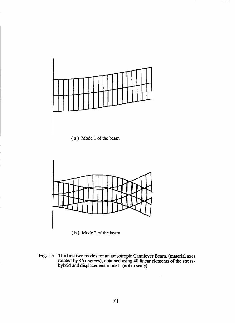
( a ) Modelofthebeam
( b ) Mode2ofthebeam
Fig. 15 The first two modes for an anisotropic Cantilever Beam, (material axes rotated by 45 degrees), obtained using 40 linear elements of the stress- hybrid and displacement model (not to scale)
71
1 . 2 ~ - 1 .o
0.2 -
0.8 4 a' -anal 0.61
-fern
-Q Hybrid elem. * Displ. elem.
0.0 I. 1
2 4 6 8 10 12 No. of Elements
( a ) 1st Natural Frequency
1 1 . 2 ~ - .o
Q Hybridelem. * Displ. elem.
2 4 6 8 10 12
No. of Elements
( b ) 2nd Natural Frequency
Fig. 16 Convergence of the first two Eigen values using 8-noded quadratic elements for Hybrid and Displacement models - Isotrpic case
72
( a ) Modelofthebeam
( b ) Mode2ofthebeam
Fig. 17 The first two modes of an isotropic Cantilever Beam, using 10 quadratic elements of the stress-hybrid and displacement model (not to scale)
73
( a ) Modelofthebeam
( b ) Mode2ofthebeam
Fig. 18 The first two male shapes of an anisotropic Cantilever Beam (material axes roated by 45 degrees), obtained using 10 quadratic elements of the stress-hybrid and displacement model (riot to scale)
74
75
x
t
76
( a ) Modelofthebeam
( a )Mode 2 of the beam
'ig. 21 The first two modes of the tapered Cantilever Beam made up of 3 anisotropic crystals, obtained by using 10 quadratic elements of the stress-hybrid and displacement model (not to scale)
77