A static model of a Sendzimir mill for use in shape control.

GUNAWARDENE, G. W. D. M.

Available from Sheffield Hallam University Research Archive (SHURA) at:

http://shura.shu.ac.uk/19734/

This document is the author deposited version. You are advised to consult the publisher's version if you wish to cite from it.

Published version

GUNAWARDENE, G. W. D. M. (1982). A static model of a Sendzimir mill for use in shape control. Doctoral, Sheffield Hallam University (United Kingdom)..

Copyright and re-use policy

See http://shura.shu.ac.uk/information.html

Sheffield Hallam University Research Archivehttp://shura.shu.ac.uk

! * v n u J iiv iiiii I _ _SHEFFIELD S I 1VVB | jJ QO

79294-64-0, ,6

Sheffield City Polytechnic Library

REFERENCE ONLYR6297

ProQuest Number: 10697036

All rights reserved

INFORMATION TO ALL USERS The quality of this reproduction is dependent upon the quality of the copy submitted.

In the unlikely event that the author did not send a com ple te manuscript and there are missing pages, these will be noted. Also, if material had to be removed,

a note will indicate the deletion.

uestProQuest 10697036

Published by ProQuest LLC(2017). Copyright of the Dissertation is held by the Author.

All rights reserved.This work is protected against unauthorized copying under Title 17, United States C ode

Microform Edition © ProQuest LLC.

ProQuest LLC.789 East Eisenhower Parkway

P.O. Box 1346 Ann Arbor, Ml 48106- 1346

STATIC MODEL OF A SENDZIMIR MILL FOR USE IN SHAPE CONTROL

BY

G W D M GUNAWARDENE MSc

A thesis submitted in partial fulfilment of the requirements of the Council for National Academic Awards for the Degree of Doctor of Philosophy (Ph D)

Department of Electrical and Electronics Engineering Sheffield City Polytechnic Pond Street Sheffield

Collaborating bodies :British Steel Corporation Swindon House Rotherham S60 3ARGEC Electrical Projects LtdBoughton RoadRugby

September 1982

A STATIC MODEL OF A SENDZIMIR MILLFOR USE IN SHAPE CONTROL

byG W D M GUNAWARDENE MSc

ABSTRACT

The design of shape control systems is an area of current interest in the steel industry. Shape is defined as the internal stress distribution resulting from a transverse variation in the reduction of the strip thickness. The object of shape control is to adjust the mill so that the rolled strip is free from internal stresses. Both static and dynamic models of the mill are required for the control system design.

The subject of this thesis is the static model of the Sendzimir cold rolling mill, which is a 1-2-3-4 type cluster mill. The static model derived enables shape profiles to be calculated for a given set of actuator positions, and is used to generate the steady state mill gains. The method of calculation of these shape profiles is discussed. The shape profiles obtained for different mill schedules are plotted against the distance across the strip. The corresponding mill gains are calculated and these relate the shape changes to the actuator changes. These mill gains are presented in the form of a square matrix, obtained by measuring shape at eight points across the strip.

DECLARATION

I hereby declare that this thesis is a record of work undertaken by myself, that it has not been the subject of any previous application for a degree and that all sources of information have been duly referenced.

ACKNOWLEDGEMENTS

This thesis, being the result of three years of research work, naturally involves the co-operation, consultation and discussion with many people. I wish to express my gratitude to everybody concerned.

I wish to thank my supervisor and the project leader Prof. M. J. Grimble for his guidance andencouragement throughout this research work, and also to my second supervisor Dr. G. F. Raggett of the Department of rfethematics for his valuable assistance.

I would specially like to thank Dr. A. Thomson of GSC Electrical Projects Ltd., whose advice was invaluableand to Mr. K. Dutton of BSC.

Thanks are also to our indutrial collaborators at BSC and GEC specifically Mr. M. Foster and Mr. A. Kidd

FOR USE IN SHAPE CONTROL

G ¥ D M GUNAWARDENE MSc

ABSTRACT

The design of shape control systems is an

area of current interest in the steel industry. Shape is

defined as the internal stress distribution resulting from

a transverse variation in the reduction of the strip

thickness. The object of shape control is to adjust the

mill so that the rolled strip is free from internal

stresses. Both static and dynamic models of the mill are

required for the control system design.

The subject of this thesis is the static

model of the Sendzimir cold rolling mill, which is a

1-2-3”^ type cluster mill. The static model derived enables

shape profiles to be calculated for a given set of

actuator positions, and is used to generate the steady

state mill gains. The method of calculation of these

shape profiles is discussed. The shape profiles obtained

for different mill schedules are plotted against the

distance across the strip. The corresponding mill gains

are calculated and these relate the shape changes to the

actuator changes. These mill gains are presented in the

form of a square matrix, obtained by measuring shape at

eight points across the strip.

CONTENTS.

DECLARATIONACKNOWLEDGEMENTS iABSTRACT iiCONTENTS iii

1 INTRODUCTION1.1 Review of the history of rolling mills 11.2 The purpose of rolling mill research 31.3 The Sendzimir cold rolling mill 51.4 Shape control problem 8

1.5 Objectives and summary of presentation 11

2 THE SHAPE CONTROL IROBLEM2.1 Introduction 152.2 Definition and units of shape 172.3 Shape measuring devices 192.4 Shape control mechanisms 21

2.5 Disturbances to shape 222.6 Interaction between shape and gauge 232.7 Description of the mill 232.8 Elementary shape control scheme 26

2.9 Purpose of the study 27

3 THE STATIC MODEL

3.1 Introduction 393.2 Roll bending calculation 42

3.3 Roll flattening calculation 43

iii

3.4 Roll force calculation 463.5 Output gauge and shape profile

calculations 483 .6 Brief description of the static model

computer algorithm 50

Chapter 4 COMPLETE STATIC MODEL ALGORITHM4.1 Introduction 544.2 Strip width adjustment 554.3 Strip dimensions 554.4 Back-up roll profile 574.5 First intermediate roll profile

calculation 60

4.6 Static forces in the mill cluster 6l4.7 Elastic foundation constant K 624.8 Roll force model 65

4 .9 Inter roll pressures 67

4.10 Roll deflections 714.11 Strip thickness and stress profiles 744.12 Pressure and deflection profiles for

one quarter of the mill cluster 784.13 Mill gain matrix 82

Chapter 5 STATE SPACE REPRESENTATION OF THE MILL5.1 Introduction 1035.2 Mill representation in state space form 1065*3 State equation of the complete system 1155.4 Shape profile parameterisation 118

iv

5.5

Chapter 6

6.16.26.36.4

6.5

6.6

Chapter 77.17.27.3 7 >

REFERENCES BIBLIOGRAPHY APPENDIX 1 APPENDIX 2 APPENDIX 3 APPENDIX 4 APPENDIX 5 APPENDIX 6

APPENDIX 7

Shape control system design 121

RESULTS AND DISCUSSION OF RESULTSProperties of shape profiles 130Properties of the mill gain matrix 132Shape changes for strip width variation 135The effect on gains of changing other variables 138

Shape control system diagonalisationusing singular value decomposition 142Gain matrices for different schedules 149

CONCLUSIONSGeneral conclusions 212Shape profiles and static gains 215Shape control design 218Future work 221

223230

Forces in the roll gap 235Theory on elastic foundations 24lActuator transfer function gains 250Strip dynamics 252Shapemeter time constants 254Mill transfer functions for low, medium and high speeds 255

Yield stress curve for stainless steel type 304 256

v

APPENDIX 8 The transformation matrixAPPENDIX 9 Copies of published papers

Errata

p45 Line -9 Replace "eq.(3.6)” by ”eq.(3.7)"

p71 Eq. 4.53 Replace ” q = ... = q(x)” by "cf = ..

p76 Eq. 4.65 Replace "h^ Q h ..." by "hn ft

p83 Eq. 4.89 Replace the limits by "M x

d97 Fig 4.14 2nd box should read y . = f(F.(x), a,a J Jp124 Line -5 Replace "U^ and V” by "V and l)""

p129 Fig 5.5 Replace "V" by "U *” and "U” , by

□140 Line 11 Replace "decrease" by "increase"

Line 12 Replace "0^ to O2" to "0^ to 02"

■ = q ( * )

vv

( i-1) "

b)

”V"

Chapter 1.

INTRODUCTION.

1.1. Review of the history of rolling mills.

First evidence of a possible attempt to design a cold rolling mill appears in a sketch byLeonardo da Vinchi1. The machine was built later to stretchand roll copper strips of sufficient evenness and thinness, for the making of mirrors. The history of rolling records the construction of a hand mill for lead rolling in 1615. Nearly a century later there were various plate millspowered by water wheels or horses for rolling lead andcopper. By around 1700, reasonably large mills were inoperation for rolling hot ferrous metals. The idea of thethree - high mill for rolling metal was more than acentury old before it was first introduced into iron works in Sweden in 1856 and in England in 1862. Its inventor,Christopher Polheim had realised the value of being ableto pass the metal back and forth without having toreverse the rolls.

Another idea from the previous century, thecontinuous mill, had been patented by William Hazeldine in1798, but was not used until it was reinvented by GeorgeBedson in 1862. Here the metal was fed successively intoa series of roller stands placed in line so that itssize was reduced.3

- 1 -

The development of rolling mills has continued at a high increasing rate from 1920*s onwards. Today there are a wide range of mill configurations and associatedequipment to suit all applications. The period of greatest evolutionary change, which spans the last fifty five years,

can be divided into three distinct periods: first generationmills from 1927 to i960, second generation from 1961 to I969 and third generation from 1970 to present day!

Up to i960, strip mills operated at low speeds (with exit speeds not more than 12 m/s) and handled small coils weighing up to about 10,000 kg. From i960 the progress was rapid and the second generation mills were designed to deal with heavier coils and at faster speeds.By the end of the decade automatic gauge control was introduced to meet the more demanding market. The third generation mills emerged in response to the need to roll much larger coils. These mills were capable of handling 45,000 kg coils at speeds up to about 29 m/s.

Major requirements of rolling may be outlinedas increasing coil sizes, gauge and shape performance, and led to many new developments. These include the introductionof more stands per tandem mill, improved automatic gauge control systems, hydraulically loaded mills, automatic roll changing, strip threading and coil stripping facilities and continuous rolling.5

- 2 -

The development of computers helped the automation of tandem mills. The first computer controlled mill was commissioned at British Steel Corporation, Port Talbot, England in 1964. This was followed by a chain of developments of computer controlled mills, with the objective of obtaining good shape and accurate gauge. The subject of automatic gauge control and shape control became more important in computer control development with the application of shape measuring devices6.

1.2. The purpose of rolling mill research.

Rolling first started with hot materials, with the knowledge of how to obtain a desired result. In many cases the reasons were unknown and the practical knowledge was more advanced than the theory. Weaknesses and defects of rolling were discovered through failures, and succesful designs were produced by improving the faulty parts. This experience of success through failure stimulated the understanding of rolling, such as what happened to a material when it passed between rolls, what forces were required to deform it, etc. The knowledge was needed by the designer to estimate, for example, the stresses in his machine, and by the operator to produce his product as cheaply and efficiently as possible.

Later, when cold rolling was introduced, a new set of problems had to be faced, since the requirements of the rolling process was to produce materials reasonably flat and

- 3 -

of uniform thickness across the width and length of thematerial. This required that the screwdown mechanism wascarefully adjusted for each pass and that the rolls weremaintained in good condition with the right shape. Whenrolling at high speeds, the rolls became heated and lost their shape, so that temperature control of the rollsbecame necessary. The lubricant to use on the strip demanded further investigation, and the best type to use for a given case is still a matter for experiment.

Materials also began to be rolled in theform of very long strip, so that it had to be wound ondrums driven from the mill. Front and back tensions were introduced to obtain a better product. These tensions affected the performance of the mill and suitable valueshad to be found by experience.

The friction forces between two rolls, and between work rolls and material cannot be directly measured. It was found, by experience, that the pressure required to deform the material between the rolls is much greater than that needed for a similar reduction between flatfrictionless plates, owing to the friction effects. It wasalso found that the pressure varies with the thickness ofthe material. Vertical plane sections of the materialbecame distorted in an almost unpredictable manner and thematerial was found to spread laterally in addition to thelongitudinal spread. The amount of spread was found to be

- 4 -

dependent not only on the dimensions and type of material used, but also on the diameter and surface conditions of the rolls, rolling speed, etc. To understand these it was necessary to develop the mathematics of rolling.

In addition to these, new materials, higheroutputs, lower rolling costs, better products with uniform gauge, etc., demand more knowledge of the principles underlying rolling. The functions of rolling mill research are to provide this knowledge and to show the ways of improvement!

1.3. The Sendzimir cold rolling mill.

The Sendzimir cold rolling mill has achieved recognition throughout industry in rolling ferrous and

gnon-ferrous metals. Sendzimir mills axe cluster mills and they differ fundamentally from conventional mills. This fundamental difference is the way in which the roll separating forces are transmitted from the work rolls, through the intermediate rolls to the back-up assemblies, and finally to the rigid housing. As this design permits the support of the work rolls throughout their length,deflection is minimised and extremely close gauge tolerances can be acheived across the full width of the material being rolled. In comparison to Sendzimir mills, the rigidity of conventional mills is governed by the size of the workrolls and the back-up rolls, which are supported by their

- 5 -

necks in two separate housings. Under rolling pressures this results in roll deflection and therefore thicknessvariation, especially near the centre of the strip.

The housing of Sendzimir mills is designed todeflect uniformly across the entire width of the mill. It provides continuous backing to the roll cluster and has the heaviest cross section at the centre of the mill where the forces are greatest. It also has short heavycolumns to carry the roll separating forces which makesthe mill very rigid. This makes it possible to produce strips with extremely close tolerances across and throughout the length.

All bearing shafts (see fig.l.l) of Sendzimirmills have concentrically mounted roller bearings and are located eccentrically in saddles. A cross section of one is shown in fig. 1.2. By rotating the bearing shafts, theposition of the backing bearings can be changed with respect to the housing, to closely control the distance between the work rolls. This is the basic control movement of the mill that permits accurate positioning of its rolls.A detailed description is given in section 2.7.2.

On Sendzimir mills crown control adjustmentoperates on the top backing bearings. It is known as "As-U-Roll" crown adjustment and is actuated hydraulically from the operator's desk while the mill is running.As-U-Roll operation is described in detail in section

2.7.3.

- 6 -

Another feature of Sendzimir mills is the capability of using small work rolls. Small work rolls are subject to less flattening and can continue to reducemetal even after it has become work hardened and verythin. This means that the mill is capable of rollingharder metals without intermediate annealing. Another advantage of the small rolls is that tungsten carbide rollscan be used economically. Rolls of this material produce high standard surface finish and maintain it over long production runs. Small rolls can be changed very easily and quickly so that strip of various widths and finishes can be rolled without stopping the mill for long periods of time.

On Sendzimir mills, lateral adjustment of the first intermediate rolls provide a means for rolling strip of various widths with a minimum of set up time, (see section 2.7.4). These intermediate rolls are furnished with tapered ends and this exclusive feature adds greatly to the flexibility of the mill.

When rolling materials like stainless steel the rolls and the strip get extremely hot due to friction effects. Recirculating coolant is used to lubricate and coolthe roll gap, rolls and backing bearings of the mill. The main cooling of the mill is done at the roll gap byusing high pressure sprays. In general, the flow of thelubricant is directed from the centre to the outside edges

- 7 -

of the strip so that the lubricant would wash away anyloose particles of the metal being rolled. One of the requirements for good operation of the mill is good filtration of the lubricant and good maintenance of thefilters. Normally the coolant system consists of a dirtylubricant tank, pumps to send the lubricant to filters, a clean oil tank and pumps to send the lubricant to the mill.9

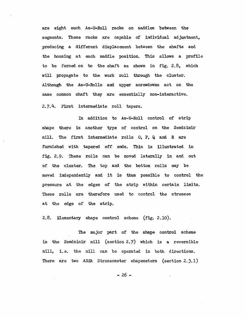
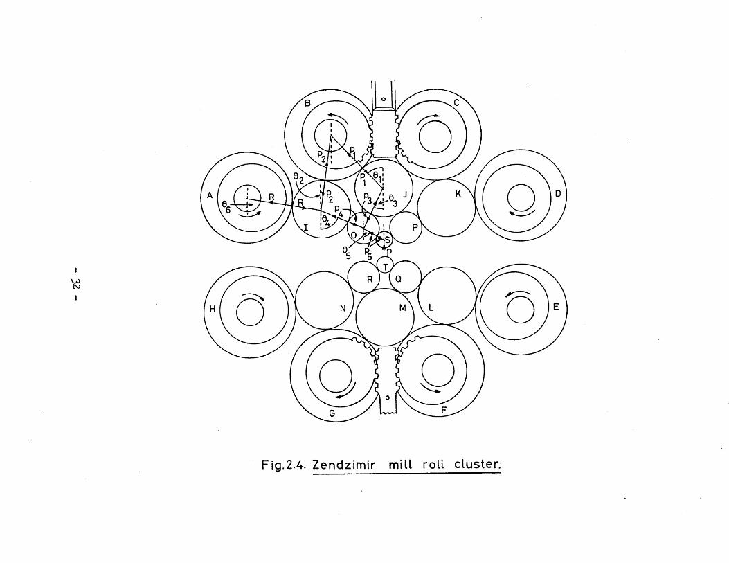
There are several different types of Sendzimir10mill and the four basic types are shown in fig. 1.1. The

subject of this study is the type 1-2-3-4 Sendzimir millwhich is the most powerful and most flexible. The rollcluster contains twelve rolls and eight backing bearing assemblies as shown in fig. 2.4. The type 1-2-3-4 millalso varies with size, and are used to roll differentdimension strips. In particular this study is concerned with a1.7 m wide type 1-2-3-4 mill which is situated at British Steel Corporation Stainless, Shepcote Lane, Sheffield, England.

1.4. Shape control problem1.1"”18

Shape describes a deviation from flatness in sheet or strip of metal. The change in demand from sheetto coil experienced by wide strip produced over the past fifteen years has brought about the need for good shape to be acheived during continuous strip processing. The demandson shape for domestic products such as washing machines,

- 8 -

fridges, freezers, etc., are most severe.

Shape is the second largest single cause for the rejection of cold rolled steel strip. Bad shape is often caused by the mismatch between the roll gap profileand the incoming strip thickness profile. This can produce transverse variations in thickness (or variations in reduction of thickness across the width) which resultin differential elongations across the width of the rolled strip. These differences can be accommodated only by large internal stresses within the strip which may cause local elastic buckling. Shape is related to internal stresses of the strip and shape is defined as the internal stress distribution due to a transverse variation in thickness reduction. The strip is said to have good shape when the internal stress distribution is uniform (see sections 2.1 and 2.2). Hence shape control refers to control of internalstress distribution across strip width when undergoing a thickness reduction.

The assessment of shape during rolling was simple when waves and the profile of ends could be seen in strips. The changing pattern of reflections on the surface may allow the deviation of flatness to be detected and the effect of corrective actions to be judged. However,with increases in strip tension, speed, coolant supply and enclosure of rolling mills, the observation is often unreliable. An instrumental method of detecting shape has

- 9 -

thus became desirable and essential for closed loop control. It was only in the last fifteen years that reliable shape measuring devices have become commercially available and the situation with shape control is now rapidly changing.

It has been well known that transverse variations in thickness are associated with bad shape and cambered rolls were used to counteract the mismatch between roll gap profile and the incoming thickness profile. Ithas been suggested that roll deflections should be minimised, to correct shape defects, by reducing roll force with smaller work rolls and backing them with stiff support rolls. It has also been suggested that roll force should be maintained constant at the correct value to match camber and that thermal camber should be minimised by efficient cooling. Strips may have localised bad shape due to uneven coolant application causing hot bands on the rolls and this may be remedied using efficient coolant distribution.

Tension can correct bad shape during rolling, but its effectiveness is not prominent, and it must be kept well below the yield stress to avoid fracture. By regulating screw-down settings, tension or speed it is possible to adjust roll force and deflection, but this action may affect the mean gauge as well as the transverse gauge variation. The resultant effect on shape is judged by the operator and he will attempt to choose a suitable

- 10 -

corrective action for improving flatness as well as gaugeuniformity.

One of the main obstacles for automaticclosed loop control of shape was the commercial availability of reliable shape measuring devices. In the last fifteen years this has been overcome and reliable shape meters are available as shape monitoring element. The design of closed loop shape control systems became the current interest in the metal rolling industry.

1.5. Objectives and summary of presentation.

The first requirement in the design of ashape control system for a rolling mill is a model ofthe mill. Both static and dynamic models are required forthis purpose. The static model is used to calculate thesteady state gains which will then be used in the dynamicsimulation. The main objective of this study is thedevelopment of the mill model which represents the roll

19cluster and the conditions within the roll gap.

The shape problem is discussed in chapter two. The definition and units of shape are given and shape measuring devices are discussed briefly. A detaileddiscription of the Sendzimir type 1-2-3-4 mill is also given.

Chapter three describes the basic foundationsof the static model and in chapter four the complete

- 11 -

static model algorithm is discussed. A discussion of the state space representation of the whole shape control system is also given in chapter five. The static model results are presented and discussed in chapter six and some suggestions for improvement of the model are also given.

- 12 -

Backing bearing

- Bearing shaft -

(a ) 1-1 mill (4 high) (b)1-1-2 mill (e high)

Backing bearing

Bearing s haf t

(c) 1-2-3 mill (12 high) (d) 1-2-3-4 mill (20 high)

Fig. 1.1. Typ es of Sendzimir mill.

- 13 -

Eccentric ring

Backing bearing

Bearing shaf t

Foot of the sadd le

Fig. 1.2. Cross section of a bearing s h a f t

showing eccentr ic r ings.

Chapter 2.

THE SHAPE CONTROL PROBLEM.

2.1. Introduction.

In recent years, the problem of the controlof the gauge of steel strip leaving a rolling mill, has

20largely been solved. The major problem of current interest in cold rolling mills involves the control of internal

21— 27stresses in the rolled strip. This is referred to asshape control, a term which often causes confusion. Stripwith good shape does not have internal stresses rolled intoit. When such a strip is cut into sections, they shouldremain flat when laid on a flat surface. Shape measurement is generally a difficult problem, since the strip is normally rolled under very high tensions which makes theshape defects not visible to the naked eye. It is only in the last fifteen years that reliable shape measuringdevices have become available and this has enabled recent work on shape control to progress to the closed loopcontrol stage.

To illustrate how bad shape might ariseconsider a strip having an entry gauge profile of uniform thickness. Assume also that the work roll has a profilesuch that the diameter of the work roll at the centre islarger than at the edges (barrel shape). When a strip having uniform thickness is rolled using the work roll

- 15 -

described above the reduction of thickness at the centre ofstrip will be greater than at the edges, assuming thatthere is no lateral spread. Since strip is one homogeneous mass such differential elongations cannot occur and internal stresses result. Clearly if the strip is to be flat after rolling, the reduction of thickness as it passes throughthe roll gap must be a constant across the strip width.

Shape may be defined as the internal stressdistribution due to a transverse variation of reduction ofthe strip thickness. There are two types of bad shape. Ifa section of strip is sufficiently stiff to resistdeformation the strip may appear to have good shape, butlatent forces will be released causing deformations duringslitting operations. This type of bad shape is referred toas latent shape. Hie second type of bad shape is calledmanifest shape, where thin strip having insufficient strengthto resist forces imposed, exhibits bad shape in the formof waves or ripples extending along the length of the

12strip and covering the whole or part of the width. Thesetwo types of bad shape are illustrated in fig. 2.1.

The stress distribution patterns giving riseto bad. shape may be tensile or compressive in nature. Theactual appearance of buckling will depend upon the

28distribution of stresses and some examples of manifestshape known generally as long edge, long middle, herringbone and quarter buckle are illustrated in fig. 2.2. Long

- 16 -

edge and long middle arise ftrom- fairly elementary stress configurations. As the strip thickness decreases the latent stress capacity decreases and hence manifest shape defects are more often observed. Frequently these appear in complexforms such as herring bone and quarter buckle.

Deformations such as long edge and long middle are caused by the mismatch between the strip and roll gap profiles under rolling. The factors which affect

29strip shape may be listed as:1. Incoming hot band strip profile,2. Roll separating force and its effect on roll

camber,3. Strip entry and exit tensions,4. Slip in the roll gap.

2.2. Definition and units of shape.

Shape may be defined as the internal stressdistribution due to transverse variations of reduction of the strip thickness. The transverse variation in the longitudinal stresses is caused by the transverse variations in the slip and hence the strip velocity at the exit ofthe stand (or at the entry to the next stand in amultistand mill).

14Pearson has defined a unit of shape calledthe •mon* in terms of the classical long edge or longmiddle defects. Pearson relates shape to the amount of

- 17 -

bowing present in narrow bands slit from the strip. Themon defines the shape of strip which if slit into bandsof 1 cm wide, would produce a lateral curvature corresponding

/fto a radius of 10 cm. If this definition is applied to a long edge or long middle defect, the shape in mons isthe fractional difference in elongation between the centreand edge of the strip multiplied by a factor of 10 .That is, let A^ represent the difference in length between the longest and shortest line segments of the strip, then

mons = — .10** (2.1)t

For example, for 0.01 % elongation A-#/# = 0.0001 and thisequals one mon unit. The strip shape may be defined as the relative length difference per unit width expressed inmortem. That is

Shape = ~r"~~ *10** modern (2.2)I ws

where w is the width of the strip in cm. For most sapplications a shape of 0.05 moi^cm is considered very good and a shape of 1 mon/cm is considered very bad in rolling strip.

30Sivilotti et al define another unit for shape called I units. It is defined as

I unit = -1^5 (2.3)V

- 18 -

2.3. Shape measuring devices.

The lack of a good shape measuring device for many years frustrated the proper control of flatness of strip. As compared to gauge measurement, shape is rather difficult to measure. The strip tension between the last stand and the coiler is usually high and therefore the strip appears perfectly flat (latent shape). Here thevisual inspection is no use and is little help to theoperator who has to decide whether the shape is acceptable or not. Therefore a reliable measuring device which indicates the shape was required. It was only in the last fifteen years that reliable shape measuring devices have become commercially available and have been applied in thesteel industry. Due to this fact the situation with shape control is now rapidly changing.

There are various types of shape measuringdevices. The most successful and reliable devices seem to

31be the Leowy Robertson Vidimon shapemeter and the ASEA.32.34Stressometer shapemeter. The Japanese have already applied

35,36the former to open loop control on a Sendzimir mill. However the latter device will be considered here since this is the instrument employed on the steel mill ofinterest.

1 2 ,21,222.3.1. Principles for shape measurement.

Only two practical basic methods are availablefor shape measurement. The first method which can be

- 19 -

applied to magnetic materials, uses the fact that magnetic permeability of ferromagnetic materials changes with stress. This system consists of two U-shaped iron cores, where one core is magnetised with alternating current which induces a magnetic field in the strip. The other core is used for sensing the magnetic potential difference between two points in the field, which will produce an output voltage proportional to the local stress without touching the strip.A set of devices spaced across the strip or one single device moving across the strip will produce a measurement of strip stress distribution.

The second method uses a device which deflects the strip a certain angle by means of a roll and measures the deflecting forces on a number of measuring zones.

2.3.2. ASEA Stressometer.

The ASEA Stressometer shapemeter uses the second method mentioned above. The stressometer measuring equipment consists of a measuring roll, a slip ring device, an electronic unit and a display unit. A schematic diagram is shown in fig. 2.3. The measuring roll is divided into a number of measuring zones (for the Sendzimir mill 31 zones) across the roll, and the display unit has the same number of indicating panels. Stress in each section of strip is measured in the zone independent of adjacent zones. A condition for this independence is that the whole roll assembly and the individual measuring zones are very much

- 20 -

stiff er than the curved part of strip. The sensors are aform of magnetoelastic force transducer and these are placed in four slots equally spaced around the roll periphery. Theperiodic signals from each zone are filtered and the stress in each zone is calculated. The average stress is alsocalculated and the deviation of actual stress from the mean is displayed on corresponding display units. To obtain thebest possible representation of the actual stress distribution,it is required to arrange the measuring roll and coiler parallel to the roll gap. Any deviation from this willintroduce false stress profiles superimposed on the true profile.

2.4. Shape control mechanisms.

The main task of any shape control scheme isto produce a strip with low transverse variation of stressat the mill exit. The shape can be affected either by

37changing the roll deformation, by changing the roll profile,or by changing the thickness profile of the ingoing strip.Roll deformation can be changed either by varying the reduction or by applying bending forces to roll bending mechanisms. It is usual to maintain the correct exit gauge and thence the reduction must be kept constant. Thus roll bending mechanisms are used to affect the shape. Anotherfactor affecting the shape is the strip tension. Byaltering the strip tension, the roll force can be changed which in turn changes the roll gap profile.

- 21 -

Another method sometimes used is to change thethermal camber of the rolls. The thermal profiles developedon the rolls during rolling are due to friction and theheat input across the strip width in the roll gap. Byvarying the amount and/or distribution of the coolant ondifferent parts of the rolls, the thermal expansion andhence the strip shape can be modified. Coolant spraycontrol has the advantage that it can produce a widerange of roll profiles. Ibis type of control has a longtime constant, sometimes several minutes, which can be a

38disadvantage. Regulation by tension and roll bending can clearly be faster than the action of the thermal camber control. Regulation by tension, though it is faster, is limited by what additional tensile stress the strip can sustain. The comparative efficiency of these methods still remains to be investigated.

2.5. Disturbances to shape.

Changes in mill entry gauge profile can be considered as one type of disturbance to shape. Another disturbance would be due to changes in roll force followingfrom changes in the mean entry thickness of strip, hardness or friction. Changes in friction or the properties of thecoolant may cause a change in thermal camber which also can be considered as a disturbance to shape. Changes in the thermal profile will always be slow. Roll wear, which

- 22 -

is very gradual, is also a problem in shape control.

2.6. Interaction between shape and gauge.

If a gauge error is corrected by the screwdownthen the total rolling force changes the resulting shape.If a shape is corrected by adjusting tension then again roll force changes affect the gauge. On the other hand ifshape is corrected by roll bending, then in addition to achange in the distribution of rolling pressures, the overall pressure between work roll and back-up roll willchange altering their mutual flattenning. This will produce a change in the roll gap, thus affecting the gauge.

The gauge and shape control therefore always interact and a combined gauge and shape control system is required to be effective. However, since shape control systems are often added to existing steel mills, this isnot always possible. In this study the effect of thegauge control loop will be neglected.

2.7. Description of the mill.

2.7.1. General description of the mill.

There are various types of Sendzimir mill.The mill considered here is 1.7 m wide and is a clustermill where the work rolls rest between supporting rolls.The mill has eight backing shafts labelled A to H, sixsecond intermediate rolls (I to N), four first intermediate

- 23 -

rolls (0 to R) and two work rolls (S to T) as shown infig. 2.4. This type of mill is used for rolling hardmaterials such as stainless steel.

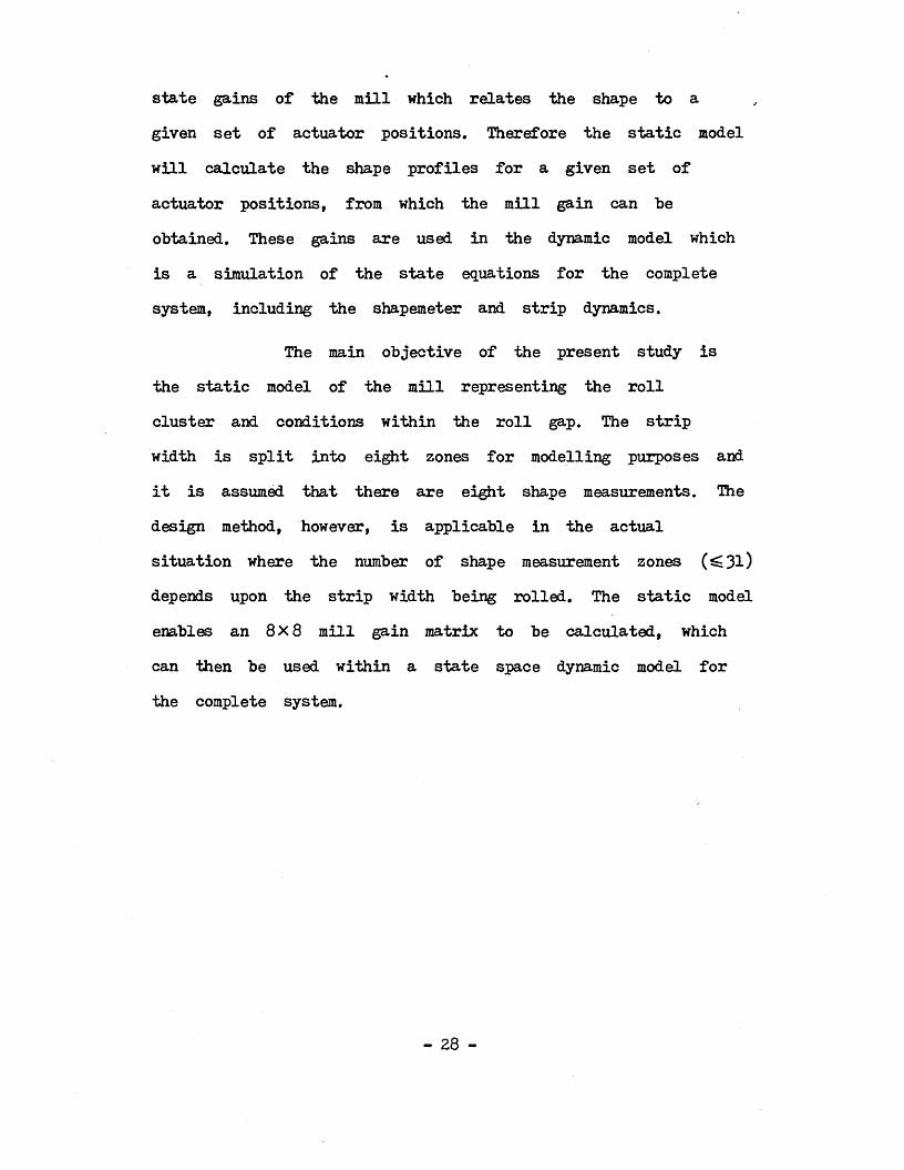
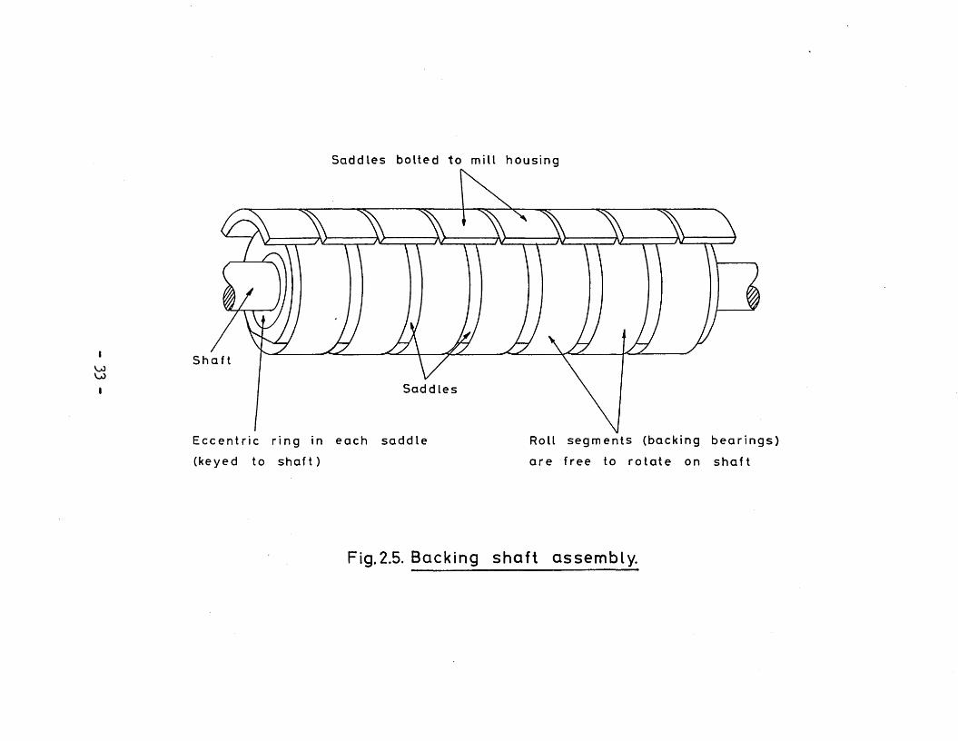
The motor drive is applied to the outersecond intermediate rolls (I, K, L and N) and the transmission of the drive to the work rolls via the first intermediaterolls is due to inter roll friction. Rolls labelled I to Thave free ends and are free to float. The outer rolls (Ato H) are split into seven roll segments as shown in fig.2.5. The shafts in which these rotate are supported byeight saddles per shaft, positioned between each pair of roll segments and at the shaft ends. The saddles arerigidly fixed to the mill housing. The saddles containeccentric rings. The outer circumferences of these rings arefree to rotate in the circular saddle bores, while the inner circumferences are keyed to the shafts.

2.7.2. Upper and lower screwdown operation.

The upper screwdown racks act on assembles Band G, while assemblies F and G are responsible for the lower screwup system. Ehch saddle of the assemblies B and Gis constructed as shown in fig. 2.6. The saddles on theF and G assemblies are also constructed in the same waybut without the As-U-Roll eccentric rings. When the shaft is rotated, the eccentric screwdown ring also rotates in the saddle bore, since it is keyed to the shaft. This allows the centre c^ of the shaft to rotate about the centre c^

- 24 -

of the saddle bore, thus causing a nett movement of the shaft towards or away from the mill housing. Since theshaft is keyed to the screwdown eccentric rings in alleight saddles, the same motion will occur at each endand the shaft will remain parallel to the mill housing. Essentially, the screwdowns cause the movement of rollsI, J, K, 0, P and S up or down which enables the distancebetween the two work rolls to be adjusted finely during rolling. A similar operation takes place at the lowerassemblies F and G, which is used principally for rollchanging and mill threading.

2.7.3* As-U-Roll operation.

In addition to the screwdown system, theupper shaft assemblies B and G contain further eccentrics, which allow roll bending to take place during rolling to adjust strip shape. Such a facility is referred to as the •As-U-Roll\

Each of the saddles supporting these two shafts is fitted with an extra eccentric ring (fig. 2.6) situated between the saddle and the screwdown eccentricring. This eccentric ring can be rotated independently tothe shaft and screwdown eccentric ring, by moving a rack which operates on two annular cheeks fitted on each side of this extra ring, as shown in fig. 2.7. Such a rotation will cause the centre c^ of the inner bore of this ringto move in a circular path about the centre c . There

- 25 -

are eight such As-U-Roll racks on saddles between the segments. These racks are capable of individual adjustment, producing a different displacement between the shafts andthe housing at each saddle position. This allows a profile to be forced on to the shaft as shown in fig. 2.8, whichwill propagate to the work roll through the cluster.Although the As-U-Rolls and upper screwdowns act on the same common shaft they are essentially non-interactive.

2.7.4. First intermediate roll tapers.

In addition to As-U-Roll control of stripshape there is another type of control on the Sendzimir mill. The first intermediate rolls 0, P, Q and R are furnished with tapered off ends. This is illustrated infig. 2.9. These rolls can be moved laterally in and outof the cluster. The top and the bottom rolls may bemoved independently and it is thus possible to control the pressure at the edges of the strip within certain limits.These rolls are therefore used to control the stresses at the edge of the strip.

2.8. Elementary shape control scheme (fig. 2.10).

The major part of the shape control scheme is the Sendzimir mill (section 2.7) which is a reversible mill, i.e. the mill can be operated in both directions.There are two ASEA Stressometer shapemeters (section 2.3.1)

- 26 -

on either side of the mill to measure the shape of theoutgoing strip from the mill. Only one shapemeter is in operation at any particular pass. There is a decoiler which feeds the strip to be rolled into the mill. Thepurpose of the coiler is to roll the outgoing strip into a coil. When the mill is operating in the reversedirection the actions of decoil er and coiler areinterchanged.

Between the coiler and the shapemeter, thereis a third roll called the deflector roll. As the stripis rolled the coiler diameter is increased which changes the shapemeter deflector angle. The purpose of the deflector roll is to keep the deflector angle constant so that the shape is measured relative to this constantdeflector angle.

There are two X-ray measurement devices on either side of the mill which measure the input and output mean gauge of the strip. In addition there is acontrol computer and an operator desk with the shape display unit. The basic scheme is illustrated in fig. 2.10.

2.9. Purpose of the study.

The first requirement in the design of a shape control system for a cold rolling mill is a model of the mill. Both static and dynamic models are required for this purpose. The static model must provide steady

- 27 -

state gains of the mill which relates the shape to a given set of actuator positions. Therefore the static model will calculate the shape profiles for a given set of actuator positions, from which the mill gain can be obtained. These gains are used in the dynamic model which is a simulation of the state equations for the complete system, including the shapemeter and strip dynamics.

The main objective of the present study isthe static model of the mill representing the roll cluster and conditions within the roll gap. The strip width is split into eight zones for modelling purposes and it is assumed that there are eight shape measurements. The design method, however, is applicable in the actual situation where the number of shape measurement zones 3l)depends upon the strip width being rolled. The static modelenables an 8x8 mill gain matrix to be calculated, which can then be used within a state space dynamic model forthe complete system.

- 28 -

Latent shape on subsequent

sl it ting along edge or middle

Manifest shape

with long edges

Fig. 2.1. Various forms of shape defect

- 29 -

(/)co■*->DJD-■o

- 30 -

Long edge Long middle Herringbone Quarter buckle

Fig. 2.2. Manifest buckling forms.

Display unit

a.CO

XJ

h-

- 31 -

Fig. 2.3. Schematic diagram of Stressometer shapemeter.

- 32 -

Fig .2.A. Zendzimir mill roll cluster.

Saddles bolted to mill housing

WcnTJsz

sz

oo *

iLl wjCto- 33 -

Fig.2.5. Backing shaft assembly.

cnccnc

w ~ * ° Scn 'Z c a

cnJCn

TJTJCM

- 34 -

Fig .2.6. Saddle detail shafts B and C (not to scale).

X

>*\jQE)U)V)d

0 cn13ICO<c<CsJcn

- 35 -

ivi U U Lvwl U twJ □

2nd Intermediate roll

1st Intermediate roll

work rol l

(a) A s -U - R o l l racks before motion

TU

2nd Intermediate roll

1st Intermediate roll

work ro l l

(b ) A s -U - R o l l racks a f t e r motion

Fig. 2.8. E xam p le of A s -U -R o l l action.

- 3 6 -

- 37 -

o

cn

jC

o O'*

CL<L> *U CL

O

J—

C

cncnck_Z3(Aa<b£

-oQl

CL

~oX)o£ou.

- 38 -

Fig.2.10. Schematic diagram showing the basic components in the system.

Chapter 3*

THE STATIC MODEL.

3.1. Introduction.

The study of any scheme for control of stripshape must he preceded by an accurate analysis of theformation of the loaded roll gap in the rolling stand. A

39static model for the single stand Sendzimir cold rollingmill is described in this chapter, which provides acomplete analysis of strip shape. The static model is amechanical model for the mill which represents all forcedeformation relationships in the roll cluster and in the roll gap. It is important for control purposes to note thatthese relationships are both non-linear and scheduledependent.

The static model must allow for the bendingand flattening of the rolls in the mill cluster and forthe plastic deformation of the strip in the roll gap. Themodel should provide

(a) mill gains between actuator movements and stripshape changes based upon a small perturbationanalysis,

(b) details of the degree of control which may beachieved with a given shape actuator or the firstintermediate roll tapers and

(c) an understanding of the mechanisms involved in the

- 39 -

roll cluster and the roll gap which affect strip shape.

The model was developed in the form of a Fortran computer program. The model enables the outputshape profile to be calculated corresponding to a givenset of shape actuator (As-U-Roll rack) positions and hence the change in shape for a given change in actuator positions; model also enables the shape change due toa change in the roll cambers to be calculated. Such a change can result from movement of the first intermediate rolls.

There are four main sets of calculations involved in the model which may be listed as followsj

1. Roll bending calculation: This is based on the40theory of beams on elastic foundations. This is

justified, as in the mill cluster, rolls rest oneach other and will be deflected due to elastic properties under loading conditions.

2. Roll flattening and inter roll pressure calculations:This enables the roll flattening between two rolls to be found for a given pressure distribution. Thepressure distribution itself depends on rollflattening and hence this calculation is iterative.

3. Roll force calculation: This enables the roll forceto be calculated for given strip dimensions and properties.

- *to -

k. Output gauge and shape profiles calculation: Thisdetermines output gauge and shape profilescorresponding to inter roll pressure and deflection profiles.

The assumptions made in deriving the staticmodel described may be listed as:

1. Elastic recovery of the strip may be neglected.2. Horizontal deflections of rolls may be neglected.3. The centre line strip thickness is assumed to be

specified.The mill is symmetrical about a line passing through the work roll centres (this need not be the case if the side eccentrics are set differently).

5. Strip edge effects may be neglected.6. Deflections due to shear stresses may be neglected.

The first assumption is justified as smallwork rolls are used in the Sendzimir mill, which limit the arc contact and give small roll gap angles. The workrolls are laterally supported by the roll cluster andtherefore there are no appreciable deflections of rolls in the horizontal direction, hence the second assumptionfollows. Because shape control depends on the profile ofthe loaded roll gap, it is assumed that the stand isoperating under automatic gauge control and assumptionthree follows.

The strip is normally placed at the centreof the mill so that the strip' width is symmetrical about the line passing through the work roll centres. The sideeccentrics are used to adjust the roll gap and for normaloperation both side eccentrics are moved by the sameamount and hence the fourth assumption follows. The fifth assumption is made to simplify the calculations and this is one of the areas where improvements have to be made. The sixth assumption is justified as the deflection of a beamdue to shear forces is- very small compared to that dueto bending forces.

3.2. Roll bending calculation.

It is well known that if a force is appliedto a beam supported at two ends, the reactions at the ends and the deflection of the beam can be calculated using simple beam theory. If the beam is resting upon anelastic foundation, where the whole length of the beam isin contact with the foundation, the deflection of the beammay be calculated by assuming that the deflection isproportional to the reaction at that point. All the rollsin the middle of the mill cluster are resting upon oneanother and since these rolls are elastic bodies it canbe assumed that each roll is resting on an elasticfoundation. Thus the actual bending deflection y can becalculated as a function of the applied force F and the

- 42 -

distance x from one end of the beam; i.e. y = f(F,x). Tobe more specific if £ is the length of the roll andthe force F is applied at a point x = a, then

y ( x ) = l ± M l t U . p ( x ^ , a ) (0«=xsSa) (3-1)

where K is the foundation constant for a given roll andX is a constant given by,

X 4 [k/(4-EI)]* (3.2)

Here p(X,£,a) is a function of X and the length & anda. The gap between the unloaded roll and the foundationis denoted by Ay(x). Si. (3.1) is the solution to the differential equation,

EX-2a = F - K(y -Ay) (3-3)dx

which follows from the theory of elastic foundations?0Si. (3.1) is true only when x is less than or equal toa. Deflections of points on the beam at distances greater than a may be calculated using the eq. (3.1) but with a replaced by (4 - a) and with x replaced by (-£ - x).

3.3* Roll flattening calculation.

The calculation of the deformation which occurs between two touching rolls in the cluster, or between the work rolls and the strip, is discussed in this section. The roll surfaces may be assumed to be

- ^3 -

cylindrical, neglecting minor bending distortions. Now when two infinitely long elastic cylinders are in contact the total interference y]j?(x) c3-11 written as a function of

the load per unit length q[ (x). That is,

y12(x ) = <1 (x ) ' (G! + c2) ' lo Se52/ 3 (dj + d2)

2a7 (x).^ + C2)(3.4)

where d^ and d^ are the diameters of the cylinders and

and are two elastic constants for respective41*43cylinders. The loading along a roll is of course

non-uniform and the roll is also of finite length.However, the influence of a point load does not extend far along the roll and, neglecting second order errors,

q7 (x) may be replaced by the inter roll specific force q(x) to calculate the interference y^(x). That is,

yi2(x) = fj/aM). (3.5)

The interference y^2(x) can also calculatedusing the roll contours due to bending. If y^(x) and y2(x)

are the deflections of the two rolls respectively, then the interference y^2(x) is a function of these two

deflections. Also the interference depends upon the thermal and ground camber yQ(>0* Thus,

y ^ M = ^ ( y ^ ) . y2 (x )» yc M ) * (3.6)

- -

Now deflections y^(x) and will clearly

depend upon the pressure q(x) between the rolls and hence on y12(x). Therefore a third equation can be written for

q(x) given by,

From eqs. (3.5) and (3.7) it is seen that y ^ W depends

on q(x) and q(x) depends on y ^ O O and hence q(x) and

yi^(x) must be solved iteratively. The total pressure

across the roll width w must be equal to the applied force F for the system to be in equilibrium, i. e.,

to substitute for y ^ & O in (3*7) from eq. (3.6) and to

solve eq. (3*5) and eq. (3.6) iteratively by changing the distance between the roll centres until eq. (3.8) is satisfied to within a specified tolerance.

work roll flattening can occur. He also suggested a relatively complex method for calculating work roll flattening. However, for the present model, approximate results are used based upon the work of Edwards and

i M = fjCy^OO). (3.7)

o(3.8)

The method of calculating q(x) and y., (x) is

Orowan has previously noted that extensive

0 ASpooner. They noted that the work roll flattening was

- 43 -

slightly dependent upon specific roll force and related tothe Hertzian flattening which occurs between two elasticcylinders of the same diameter. The model proposed by themfor the work roll flattening y___(x) is given by,W s

yws(x) = [\ + t>2p(x)jyh (x) (3-9)

where" ,2/3

yH (x) « 2p(x)-C-log d2p(x)*C (3.10)

01. (3.10) is obtained from eq. (3.4) by setting = C

and d^ = d^ = d. The constants b^ and b^ are estimated

using plant test results and C i (1 - v^)/(tc E), where v is the Poison's ratio and E is the Young's modulus ofelasticity.

3.4. Roll force calculation.

The roll force calculations are an important part of the static model. The amount of reduction inthickness of the strip is related to the total load inthe mill or roll force. An extensive literature exists onthe calculation of specific rolling force p(x) as a function of input output thicknesses, input output tensions and work roll radius?5 i.e.,

P(x) = f(h1(x), h2(x),01(x),CT2(x)> R). (3.11)

- 46 -

When rolling hard materials, like stainlesssteel, very high forces must be applied. Since work rollsare elastic bodies they will be deformed and flattened at

46the roll gap. In order to calculate the roll force, including the flattening effects, an iterative procedure must be adopted because the deformed roll . radius is a

/function of the roll force. The deformed roll radius R43 47can be calculated using Hitchcock’s formula ’ given as

!'-! + « £ & (3.12)

where c is a constant,6 is the amount of reduction equal to Jh^(x) - h^x^, R is the initial roll radius.

The roll force may be calculated by solving eqs. (3.H) and (3.12) iteratively.

The disadvantage of the above approach forroll force calculation is the time the algorithm takesto converge. For modelling purposes the width of the stripis split into 25 mm sections (this is to match the physical dimensions of the back-up-roll) and the roll forcemust be calculated in each of these sections. Thus forone metre wide strip the roll force model must be made to converge forty times. The shape calculation is alsoiterative and thus all the roll force calculations must beperformed on each of the iterations of the shape algorithm.Thus, although the roll force calculation does not require

- 4 7 -

a very large computing time this is multiplied by the number of strip sections and the number of shape program iterations.

3.5. Output gauge and shape profile calculations.

The output gauge profile may be calculated once a given set of inter roll pressures and deflections are known. The shape profile then follows from the input and output gauge profiles and the input shape profile.

3.5.1. Output gauge profile calculation.

combined effects of roll bending, thermal and ground roll cambers and differential strip flattening. The change in the gauge profile due to these effects is given by

Ah^(x) = 2[yws(x) - yws] + ys(x) + yt(x) + 2ywo(x) (3.13)

where y (x) and y represent interference and meanws wsinterference between the work roll and the strip, ys(x)

and y .(x) represent the upper and lower cluster work roll

deflections and y (x) is the total of the thermal andwcground work roll cambers. The mean of the change inoutput gauge is thus given by

The output gauge profile is determined by the

(3.14)

- 48 -

and hence the deviation of the change in gauge from mean is given by

Ah^(x) =Ah^(x) -Ah^ . (3.15)

The new change in output gauge is calculated from the iterative formula

Alu + 1(x) =Ah?(x) -a[Ah?(x) -Ahu(x) (3.16)

where a is chosen to give a stable solution. The new output gauge profile is therefore given by

h2 W = h2m +Ah2 + 1(x) (3.17)

where is the specified output gauge.

3.5.2. Input and output stress profile calculation.

The new output stress profile can be calculated using the new gauge profile and the followingresult due to Edwards and Spooner:24

Acr (x) = (SE h2 «hl W h2m

- 1 +A°o(x)1 + Y

The input stress profile is given by

Acr^x) =YA<t2(x)

(3.18)

(3.19)

where

Y A V * ) - cn.(3.20)

- 49 -

and 3 is a constant (f3^b0.5)j details are described in section 4.10.

3.6. Brief description of the static model computer algorithm.

The static model program uses an iterative procedure as shown in fig. 3.1. The model includes the calculations for the top half of the cluster as well asfor the bottom half of the mill. It is assumed that themill is symmetrical about the line passing through work roll centres. The model can be used for different values of strip width but for the present analysis the rollflattening equations ignore strip edge effects. The input data required by the model may be summarised as follows:

1. Cluster angles (see fig. 2.4)2. Roll diameters

3. Roll profiles (camber, wedge etc.)4. As-U-Roll positions

5. First intermediate roll positions6. Entry gauge profile

7. Mean entry gauge8. Mean exit gauge

9. Annealed gauge10. Yield stress curve11. Entry tension12. Exit tension

- 5 -

13. Width of stripThe output data may he listed as:

1. Inter roll pressures (12 profiles)2. Roll force profile3. Roll deflections (12 profiles)4. Exit shape (stress distribution) profile5. Exit gauge profile

The mill width is divided into a number ofsection multiples of 67 and the following assumptions are made (the number 67 is chosen to match the physical dimensions of the back-up-roll and its segments).

1. The pressure distribution in each section may be calculated using a point load applied at the centre of the section and the width of thesection.

2. The mean deflection of a roll over a section istaken to be equal to the deflection at the centre of the section.

These assumptions also apply to the stress distribution,strip profile, rolling pressure profile etc.

The computer algorithm enables a change in theshape profile due to a change in the rack position, andhence the gains of the mill to be calculated. The flowchart for the main program is shown in fig. 3-1.

The program begins by initialising all thevariables and the roll force is then calculated using the

- 51 -

roll gap model. Symmetry about a line passing through the work roll centres can be assumed so that calculations arenecessary only for the left half of the mill cluster. Thesubroutine BEND calculates the pressure profiles and roll profiles of one half of either the top or bottom millcluster. If symmetry is not assumed then the routine BENDhas to be called four times to calculate all the pressureand roll profiles. At the end of each calculation of all pressure and roll profiles a convergence test is carried out on the output shape profile. The above calculationsare repeated until the error between two successive shapeprofiles is less than a predetermined value.

- 52 -

Calculate constants and initialise h^Cx), roll deflections and inter roll pressures

Calculate mean roll force p(x)

Adjust h~(x)

Call subroutine BEND to calculate roll deflections and inter-roll pressures of upper half cluster

Call subroutine BEND to calculate roll deflections and inter-roll pressures of lower half cluster

Calculate new output and input stress

profiles and a].(x)

Hasoutput stress

converged ?No

PRINT

Calculate new gauge profile h9(x)and update stress profiles

Fig. 3.1. Flow chart for the main program.

Chapter

COMPLETE STATIC MODEL ALGORITHM.

4.1. Introduction.

The complete description of the mill gain calculation is described in this chapter. Sections 4.2 to4.7 describe the calculation of mill constants. Sections 4.8 to 4.11 describe the roll force model, roll pressure and deflection calculation, thickness and stress profile calculation. The final two sections describe the complete model and the gain matrix calculation.

The mill width is divided into 67 sections or multiples of 67 sections. This odd number 67 is chosen to match the back-up roll dimensions to its segments. To be more precise, for one segment of the back-up roll (see fig. 4.1), the ratio between the portion in contact withthe second intermediate roll b to non contact area (& - b) is an integer if the mill width is divided into 67

sections. That is lengths b and (-6 - b) can be dividedinto an integer number of sections. The width of each section is given by

\

4-. 2. Strip width adjustment.

The width of the strip w has also to hesadjusted so that the strip width will have an integernumber of sections. This is done in * the following manner.The strip is placed in the mill so that the centre ofthe strip width lies on the vertical line passing throughthe mill centre. If the edge of the strip lies inside asection (see fig. 4*.2) the distance between the edge ofsection and the edge of the strip is calculated. This isdenoted by Aw .s

where (r + l) is the integer number of the section in which the strip edge lies inside.

k.J. Strip dimensions.

either rectangular or parabolic the model considers onlythese two types of profile. If the strip centre linethickness h and the amount of strip camber h are m cspecified then the strip profile can be obtained as shown

If Aw >-5-, thenS c*

ws = [(N - r - l) - (r + l)J dx = (N - 2r - 2)dx (^.2)

If Aw thens &

a 3)

Since most of the input gauge profiles are

- 55 -

below.

An equation for a parabolic profile as shown in fig. can be written as (variables defined infig. 4.3a)

y(x) = h (^.*0

As shown in fig. *K3b the thickness at any point distance x from the left hand end of the mill can be written as

h(x) = hw + 2y(x) (*•5)

= h + 2h w c i - ( It - 1>2m

= h + 2h - 2h ( — - I)2 w c cv w 7mBut

h = h + 2h m w ci. e.

h(x) = h - 2h ( — - 1 )2 ' 7 m cv w 7 *m(4.6)

If the strip is rectangular then this profile can be obtained by putting hQ = 0 in eq. (*K 6).

The input thickness profile is given by

V x> " - 2V tr - D 2m(4.7)

where the suffix 1 stands for the input side of the mill. The output thickness h9(x) can be calculated if the

- 56 -

reduction is known. This can he done by specifying the centreline output strip thickness. Let this be h^. Assuming

that there is constant reduction across strip width, h^(x)

is given by

h2w = lm

The mean output thickness is given by

therefore the deviation of output gauge from mean is given

BjL. (A. 8) assumes constant reduction which implies that the output strip has perfect shape. This is only an initialization process and the deviation Ah^(x) given by

eq. (A. 10) will be updated at later stages, since the workroll profile will be deformed when forces are applied.

A. k. Back-up roll profile.

distance the back-up roll axis is deflected. The back-up roll profile calculation for a given As-U-Roll movement is

( M )

When the As-U-Rolls are moved by a certain

- 57 -

described here. When the As-U-Roll is moved verticallyupwards or downwards the mechanics are designed in such away that the centre c^ of disc B rotates about a fixed

point c^ (see section 2.7.3) as shown in fig. 4.4a. If c

is the distance between c^ and c , the centre c^

describes a circle of radius c with centre at c . This

means that, since disc B is solid, any point on the disc describes a circular arc with radius c. Let z be thevertical movement made by the As-U-Roll. Since the disc B is geared to racks, any point on the circumference alsoexperiences a net movement of z. This point also rotates about c^ and therefore the angle of rotation 0 about c^

as shown in fig. A. 4b is given by

where R is the distance between c^ to the racks. Therefore

the net vertical distance y travelled by c^ or any other

point on the circumference is given by

On either side of each segment there are two such discs which can be moved independently. The profile of the back-up roll between two racks are calculated assuming a linear relationship. Fig. 4*. 5^ shows the profile when the first rack is moved by a distance z^ with zero movement

(4.11)

y = c-sin0 = o-sin( ). (4.12)

- 58 -

in all other racks. The profile y^(x^) can be calculated

from

where Z is the distance between two racks. Fig. 5b shows the profile when only the first and second racks are moved by distances z^ and ’ z . In this case the profiles

yi(xi) and corresponding to first and second segments

are given by

The profile for the case when alternative racks are moved by the same amount (say z^) is shown in

fig.4.5c. Fig.*h51 shows the profile when all racks are

racks are moved by the same amount then obviously the whole of the back-up roll will be moved vertically. The same result can be achieved by moving the two screwdowns situated at both ends of the back-up roll, by the same amount.

(4.14)

and

(4.15)

moved by different amounts (say z , z , Zg). When all

- 5 9 -

4.5. First intermediate roll profile calculation.

The first intermediate rolls are furnished with tapered ends (see section 2.7.4). The top and bottomrolls can be moved laterally in and out independently and therefore will have different profiles depending on the position at which they are placed. These rolls can bemodelled by defining the position of the tapered edges (vertical planes e^ and e^ in fig. 4.6) with respect to the mill.

If x is the distance from the left handrcorner of the mill to the plane e and 0 is the angleof inclination of the tapered end, then the tapered profile y^Cx) is given by

0 for 0^ x^ xy t i (x ) = -4 (4.16)

(x - x )tan0 for x < x<w .v r' r m

Similarly for the bottom first intermediate roll the taperedprofile S^ven ^y

(x - x)tan© for 0^x<xx m ' myt 2 ^ = \ (4.17)

0 for x < x<wm mwhere variables x, x and w are defined in fig, 4.6. Thesem mprofiles must be added to the camber profile (if any) to obtain the total first intermediate roll profiles.

- 60 -

4.6. Static forces in the mill cluster.

When three forces are acting on a cylinder as shown in fig. 4.7, the two unknown forces P^ and P^

can be calculated in terns of the known force P and the angles of inclination. If forces are resolved in a direction XX (fig. 4.7a) perpendicular to P^* P- can be

calculated. That is

E jc o s fk - (90 - e2 )l = Pcosje - (90 - e2 )l

i. e.sin( 0 + 0?)

f q— T~pT\ • (4.18)1 sm( 0. + 0^) v '

Similarly if forces are resolved in a direction YY (fig. 4.7b) perpendicular to P^

P^cosj^ - (90 - 01)J = Pcosj© + 90 - 0^j

1. e.

sin(0n - 0)P0 = P--~ • (^.19)2 sm(01 + 02) • v

The eqs.(4.l8) and (4.19) can be applied to obtain the static forces P , P , Py P^f P^ and R shown in fig.2.4

in terms of the roll force P. If symmetry is assumed then P^ can be written as

p5 - 255Se5 ^ 20)

- 61 -

andsin (0« + 0 p — p . 3___ 2.4 5 sin(0~ + 0^

P« = Psin(0^ - 05

3 5 sin(0^ + 0^

sin(06 - 0,2 x4 sin(02 + 06

sin(02 + 0.) R “ P4 sin(©2 + 0^)

(4. 21)

(4.22)

(4.23)

(4.24)

and finally

COS0,

P. = P1 3 cos01 (^.25)

4. 7. Elastic foundation constant K.

If two cylinders are in contact the elastic foundation constant K can be found by knowing the force applied. If the mean force per unit length is p^ then the

41 43Hertzian flattening equation ’ can be written as

y = 2Cp log m ee2/3 (d1 + d2)

4Cpm(4.26)

where the force p is proportional to y and the constantmof proportionality is the foundation constant K (eq. (4.26) is obtained by putting = C2 = G in eq. (3.4)). Therefore

- 62 -

K can be written as

2C*log°ee (dx + d2)

4Cpm

At various points in the roll cluster two rolls rest on one roll. In order to use bending equationsit is convenient to use a single equivalent value for the foundation constant. This is illustrated in fig. f. 8.

Let the deflection of roll A in the direction of P be yA« The deflection y^g in the direction P^ is

given by

yAB = yA°0S(ei " 0) (4.28)

and similarly the deflection in the direction P^ isgiven by

yAC = yAcos(0 + 02^ (^-29)

If and are the foundation constants between the

cylinder A and B, and between A and Cf respectively, then

P1 - (4-30)and

P2 “ K2yAC • ^-31>

Butp = p1cos(e1 - e) + P2cos(e + e ). (^.32)

Substituting for P^ and P^ from eqs, (4-.30) and (4*. 31) and

- 63 -

eliminating and yAG we have

p = k^ a005^ 6! ~ 0) + V acos2(0 + 02^ (^-33)

But

K= “ (4.34)yA

and we obtain

2,« \ • „ 2K = K1cos^(01 - 0) + K2cosc(e + 02). (4.35)

By applying eq. (4.35) to the mill cluster (see fig.2.4) the foundation constants for rolls I, Jf 0 and S can be written as

Kj = Kaioos2(66 - 6 ) + Kbi0082(62 + e^), (4.36)

Kj = KBJcos261 + KjjjCos2^ , (4.37)

k0 = KI0oos2(e/f - e5) + KJ0oos2(e3 + e5), (4.38)

Ks = k oscos205 + kpscos205 • (4.39)

01.(4.37) is obtained by resolving forces in a vertical direction and, if symmetry is assumed, K^j = K^j and

K0S =

- 64 -

4.8. Roll force model.

For the reasons given in section 3*4 iterative roll force algorithms are not used in the present mill

force formula which thus avoids iterative calculations. The formula is not so accurate as the algorithm described in section 3*4 this type of mill but is efficient inthe use of computer time. The error of the roll force using this method was found to be about one per cent.

The Bryant and Osborne model has equation for roll force given by

48model. Bryant and Osborne developed an explicit roll

The roll force is a function of input/output thicknesses, input/output stresses and input/output yield stresses and can be written as

P ^ 1 * ^ 2 * ^ 1 * ^ 2 * ^ 1 * ^ 2 *(4.40)

PP = o (4.41)1 - bP - 0.4ab o <o

where

Po = (k - (l + o . \ ) + Pgo ,

R = work roll radius ,

- 65 -

8 = h i - h2 ,

MV oca = e°- 1 ,o . I h, 9

a - E MO — »h

p. = coefficient of fiiction,

h = 0.72h2 + 0.281 ,

- W -= 4(1 - v2)

TIE

b = 26 - J ^ / 5)2 •

bQ = (k - a)/R6.

To calculate the roll force profile eq. (4.4l) must be solved at every point across the strip. If p(x)is the roll force profile then to obtain the requiredreduction the mean of p(x) must be equal to the meanroll force j> which is the roll force required to obtainthe specific reduction. That is,

- 66 -

/wsp(x)dx. (kAz)

s 0

Every time the roll force p(x) is . calculated itmust satisfy eq.. (4-. 4-2) and if the mean of p(x) deviates from p, then p(x) must he adjusted until eq. (4-.42) is satisfied. This can he done hy moving the two work rolls away from or towards each other. If they are moved away from each other then the distance d between their two centres will he increased, thus reducing the roll force p(x) (see fig. 4*. 9). The roll force will he increased if the work rolls are moved towards each other, that is decreasing d. The flowchart for this process is shown in fig.4\ 10.

494-. 9. Inter roll pressures.

When two elastic cylinders are in contact the total interference y ^ (x) can he written as a function of

the load per unit length q(x) as

The loading is of course non-uniform but, neglecting second is

order errors, given hyA

( 1 + c2)-iog((< 1 + d~)

e 2 ^ + C2)q(x)

- 67 -

Eg.. (4-.44) contains q(x) on the right hand side and q(x) to be calculated from the knowledge of y ^ M ? thus the

term q(x) must be eliminated from the right hand side. A new variable q^(x) is defined as

^(x) - Sfe) - i WF/j2, q

(4'.45)

where F is the rolling force, Jb is the length of the roll and q is the mean specific rolling force. Thus

yi2(x)l(x) =(^i + c2)-i°g(

r'e2/3(d1 + d2)2(Ci+ C2)qqd (x)

yi2(x)

(Cl + CZ)J log{re2/3(di + d2j2(Ci + C2)q

( k M )

Now

log.e2/3(di + d2)2(Ci + C2)q » loge[qd (x)]

as q(x) =£bq.

Thus eq. (4*. 46) becomes

q(x) = y12^X)(Ol + C2)|loge 273

2 (Ci + C2) + log0(di + d£) - loge(q)\

(4.^7)Eg. (4-. 4-7) is only true for positive values of

- 68 -

Therefore it is assumed that when y ^ M ^(x) =

The interference y ^ & O can a -so calculated

from roll "bending using roll contours. If two perfectly flat cylinders (i.e. without any ground camber), one resting on the other, are considered and if there are no forces acting on these cylinders, then y^(x) must be equal to

zero. That is y*u>(x) can tie written as

y12(x) = K*! + d2) - di2 = 0

where d^ and d^ are the diameters of the two cylinders

and d ^ is the distance between the two centres. Now let

an external force be applied to the roll 1 which is thetop roll, so that only roll 1 is deflected downwards. Ifit is assumed that roll 2 has zero deflection then the distance between the two centres must increase and, tokeep d ^ = -§-(d + d^), the roll surface must be flattened

by y^(x) the actual deflection of roll 1. Therefore the

interference y ^ M can written as

y12(x) “ tC3! + d2) - di£ + y^x). (4.49)Similarly if forces are applied so that only roll 2 isdeflected upwards the interference y^(x)» to keep the

distance between two centres the same as before, can be

written as

y ^ M = l(di + d2) " di2 ■ y2W - (4.50)

If both cylinders are allowed to deflect then y-jj?(x)

becomes

y12(x) = + d2) - di2 + yi(x) - y2(x). (4.50

If both cylinders are grounded with camber (e.g. barrelshape) then the camber profiles must be added to the interference term y-^(x) to keep d ^ “ + That is

y ^ M = l(d! + d2) - ai2 + yi(x) - y2(x)

+ yl0(x) + y2o(x). (4.52)

If the cylinders have concave camber profiles then y,0(x)

and y£c(x) will be negative in eq. (^.52).

When a roll pressure q(x) between any tworolls in the mill cluster is to be calculated the mean of q(x) must be equal to the mean q, to keep the forcebalance in the mill. The pressure q(x) can be adjusted bymoving the two rolls either away or towards each other. This is done by adjusting mathematically the term d^2 in

eq. (^.52). The pressure q(x) can be increased by decreasing ^12* -s moving the rolls towards each other. The

force balance equation is given by

- 70 ~

■wq(x)dx = q(x). (4.53)

0

The method of calculation of p(x) is to change in

eq. (4.52) to change y ^ M f and ^ence <l(x) iteratively

until eq. ( f.53) is satisfied. A flowchart for this process is shown in fig. k, 11 and the subroutine used in the computer program is called INERESS.

Jf.lO. Roll deflections.

by a point load, applied to a roll resting upon an elastic foundation is given in this section. From bending theory the deflection y is given by the differential equation

where F is the applied force and K is the elastic foundation constant. This equation is only true if the roll is in complete contact with its foundation under no load conditions. However in the mill cluster, this is not always time as one particular roll may be resting on an already deflected roll, as shown in fig. 4.12. In a case like this there will be a gap between the roll and its foundation under no load conditions; let this gap be Ay.

An expression for the roll deflection caused

dxo. 5^)

- 71 -

Then eq. (4.52) becomes

-4E l - = F - K(y - Ay)

dx= F - Ky + KAy, (4.55)

ButKAy = AF.

EJg.. (4.55) becomes

,4EI-^4 = (F +AF) - Ky (4.56)

dx

where F + A f is the equivalent total force.

The solution to the differential equation (4.56) is given by

y(x) = (F + AF).|-[b(C - D) + H(J + G)] (4.57)

where

A = sinh2(\£) - sin2(\&),

B = 2cosh(Xx)cos(Xx)t

G = sinh(X£)cos(\a)coshb) ,

D = sin(X£-)cosh(Xa)cos(Xb),

H = cosh(\x)sin(\x) + sinh(Xx)cos(\x) 9

J = sinh(X^)[sin(\a)cosh(Xb) - cos(Xa)sinh(Xb)] ,

G = sinft$[sinh(Xa)cos(Xb) - cosh(Xa)sin(Xb)j

- 72 -

X =' Kand

' “ P i,

All variables not defined are shown in fig.4-.13. The eq. (4*. 57) is only true for values of x<a. The deflectionfor distances a<x<.& can be calculated using eq. (4-. 57) but with a and b interchanged while measuring the distance from right hand end.

At various points in the roll cluster threerolls are in contact with a fourth roll as shown in fig. 4-. 8. If the deflection of roll A is required the netforce acting on A must be calculated. In direction P thenet force per unit length is given by

F(x) = P(x) - P1(x)cos(01 - 0) - P2(x)cos(0 +02). (4-. 58)

If an elemental length dx across the roll length isconsidered, then the total net force acting on dx isgiven by

Fj.(x) = F(x)dx

= [P(x) - P-L(x)cos(01 - 0) - P2(x)cos(0+02)Jdx. (4-.59)

If the roll length is divided into N such small segmentsof length dx then the distributed load can be treated asa series of point loads acting on each segment. The deflection due to one such force at the jth element, given by eq. (4-. 59), can be written as

yaj(X) + yb / x) = f(?j(x)dx» a> b) (4-.60)

- 73 -

where yaj(x) is the deflection for x^a, -s the

deflection for a < x < £ and x = a defines the point of

roll deflection, from the theorem of superposition is given

Subroutine MUMMY1 in the computer program calculates the total deflection and a simple flowchart is shown in fig. 4.14.

if. 11. Strip thickness and stress profiles.

to find the interference y (x) between work roll and stripwswas to compute the roll flattening for numerous rolling schedules, roll diameters and Young's modulus. From the results they found a strong correlation between the total roll flattening y (x) and Hertzian flattening yu(x)WS rloccurring between two infinitely long elastic cylindershaving the same diameters. They computed the ratio

yws(x)/yH(x) and- a mociel was proposed to match these

results. The proposed model is given by eqs.(3.9) and(3.10). The constants b^ and b^ are estimated using least square methods to be 0.5 and 0.325 mm/tonne respectively.

application of the force F.(x)dx (see fig.*f,13). The total

kyN

(f. 61)3 = 1

The procedure adopted by Edwards and Spooner24

- 74 -

First, the mean interference y between stripWS

and work rolls is calculated using mean roll force pwhich corresponds to the required reduction. If h^(x) is

the actual output thickness, then the change in interference corresponding to a deviation in strip thickness from h^m is

(y (x) “ y„ )» where y__(x) is the true interference betweenWS ws wsstrip and work rolls. That is the change in gauge ishigher if the change in interference is high. The changein gauge also increases with the increase of work rolldeflection. If work roll camber is included, then thechange in gauge can be written as

Ah2<» - ywW + ywoW + [yHS« - yws] (*,&)

where y (x) is the work roll camber.WO

Since there are two work rolls the effectwill be doubled and Ah^(x) becomes

Ahz M = + + + 2[ywsw - ^ - 63)

where y (x) and y fx) refer to upper and lower workwuN ' W£roll deflections.

The output thickness profile is calculated asexplained in section 3.5.1 and is given by eq. (3.17)» i.e.

h2(x) = hZm + Ah^ + 1 . (4.6*0

- 75 -

The change in output stress is calculated by24the model proposed by Edwards and Spooner given by

eqs.(3.l8) and (3.19)» using the output thickness calculated.Edwards and Spooner found p to be 0.5 and that the shapedistribution was insensitive to p. The constant Y is calculated as described below.

From the geometry of fig. 4.15 it can be easily shown that

hn ~ V R6£ * (iK65)

From continuity of mass flow

v2h2 = VA • ^ - 66)

By substituting hn from eq.. (4.65) in eq.. (4.66) we have

v2 “ vn<1 + ^ > - ^ 67)

The per unit slip is defined as

v9 - vS = ^ . (4.68)

n

From eqs. (4.67) and (4.68) the value of s is found to be

2R0s = H2 69)2

- 76 -

where

9 = — - tan n v Rb i nIR 2

H1 1 Hn = 2 + Z\i

'h2 1 ~ V kl

hl 1 “ a2//k2

(4.70)

(4.71)

(4.72)

Bis. (4.70), (4.71) and. (4.72) can be derived by consideringroll gap variables and are given in Appendix 1.

By differentiating s with respect to wehave

ds 2R d0ndo. nd5j

de„ dH2R o n nh n dH "da, d n l

(4.73)

But

dS h? n j. ^dH " 2*R n 1 + (Jr'ir. (4.74)

and

dH , i n _-_l____1da1 2|i*k - ax * (4.75)

By substituting these values in eq.. (4.73) and simplifying we obtain

dsda.

- aki-C; (4.76)

- 77 -

where

A a “ 2\1 1 + tan^ l\/ R 2 I (4.77)

Similarly

ds (4.78)2

In order that the slip variations are to remain very small we must have

As = Aal i 1 +A<T2 f § 2 = 0 - P - 79)

By substituting for ^ and in eq.. (4.79) we have

A oi = y Ao'2 (4.80)

where

2 2

*f.l2. Pressure and deflection profiles for one quarter of the mill cluster.

Pressure and deflection profiles for onequarter of the mill are calculated hy using the subroutinecalled BEND. This routine has to be called four times tocalculate the profiles of all twenty rolls. If symmetryis assumed it is only necessary to calculate only one half of the mill and therefore routine BEND is used only twice.

- 78 -

Since the pressure between two rolls depends on the interference between them, and the interference is afunction of the roll deflections which directly depend onpressure, the process is iterative. Whenever two rolls are in contact this iterative procedure must be adopted to calculate the pressure profiles. In the mill cluster every roll is in contact with more than one roll. Suppose that the first profile is obtained after satisfying a convergence criterion. In the process of convergence the roll deflectionsand pressures, other than those of the one in question, change at every iteration. On the other hand, if convergence is obtained on the second profile then the first profile may have deviated from the true value. The procedure adopted is therefore to converge the first profile and then the second profile initially, and then return tofirst and then the second until convergence is obtained onboth profiles. If other pressures are included then theprocess becomes a nested convergence procedure.

For one such pressure (e.g. q^j between rolls B

and J in cluster) the convergence procedure can be explained.First the vertical deflection yj(x) of roll J (see

fig. 4.16) is calculated using existing pressure profiles qgj(x) and qj^(x). The deflection Yj(x) is resolved into

q^j and q ^ directions and these together with yB(x) and

y^(x) are used to calculate new <lgj(x) and qjQ(x). That

- 79 -

is

<iBj M = fq(yBoosei’ yjoosei) (4.82)

and

1j0W = fq(yjoos02' *^* (4.83)

since y^ and y^ are calculated in vertical and

directions respectively. At this point a convergence test is carried out on q^j using a root mean square error

criteria. If this criteria is satisfied, the present profiles <3LB j (x ) a-nd y j ( x ) are taken as the corrected

pressure profile between B and J and the deflection of J. If a convergence has not been reached the nett force F acting on J in the vertical direction is calculated, i. e.

Using this value F a new vertical deflection yj(x) is

calculated. This is done using the subroutine MUMMT and can be written as

The new deflection y T(x) is calculated using the iterative

where a is a convergence parameter chosen to give a stable solution. The above procedure is repeated until a

F = qJ0oos62 - qBJcos9r (4.84)

yj(*) = y F)- (4.85)

formula

yj + 2(x) = yjOO - a [VjOO - yj(x)] (4.86)

- 80 -

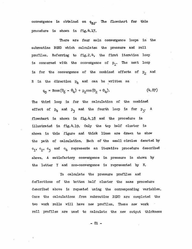
convergence is obtained on qBT. The flowchart for thisJbJ

procedure is shown in fig. 17.

There are four main convergence loops in the subroutine BEND which calculates the pressure and roll profiles. Referring to fig. 2.4, the first iteration loop is concerned with the convergence of p . The next loop

is for the convergence of the combined effects of p2 and

R in the direction p^ and can be written as

qD = Rcos (0£ - 6^) + p2cos(02 + 0^). (4.87)

The third loop is for the calculation of the combined effect of p^ and p^ and the fourth loop is for p . A

flowchart is shown in fig. 4.18 and the procedure is illustrated in fig. 4.19. 0nlY 'the half cluster isshown in this figure and thick lines are drawn to showthe path of calculation. Each of the small circles denoted by

cl* °Z9 °3 an^ °4 rePresen^s an iterative procedure described

above. A satisfactory convergence in pressure is shown by the letter Y and non-convergence is represented by N.

To calculate the pressure profiles and deflections of the bottom half cluster the same proceduredescribed above is repeated using the corresponding variables. Once the calculations from subroutine BEND are completed the two work rolls will have new profiles. These new workroll profiles are used to calculate the new output thickness

- 81 -

profile and hence the new stress profile. A finalconvergence test is applied on the stress deviation profile as shown in the flowchart of fig. 3.1 and describedin section 3.5. The convergence test carried out here isalso based on the root mean square error criterion.

39*f.l3. Mill gain matrix.

The model calculates output gauge and shapeprofiles and roll deflection and pressure profiles for agiven set of rack movements. The static gain of the mill is the ratio of the change in stress due to a change in rack position. There are eight racks and the gainsmust show the effect of shape at each point on the strip due to each rack. Therefore, the gains are calculated by changing each rack at a time by the same amount. First the stress profile is calculated by setting all the racks at a common position. Then eight new stress profiles arecalculated by changing one rack at a time by the same amount. The difference between any one of these stress profiles and the previous profile is taken as the stresschange due to that particular rack change. For computing purposes the mill width and the strip width are dividedinto a number of sections as explained in section ^.l. Therefore the gain can be represented as an N X 8 matrix, where N is the number of sections. Any element of this

- 82 -

matrix is therefore given by

A ct. .gi i = Az1J i = l,2,...N and j - 1,2,.. .8 (4.88)

5

where A ct and A z are the changes in stress and rack position respectively.

The above matrix is not a square matrix and for the use in the dynamic model it is convenient to have a square matrix. The non-square matrix can be converted into a square matrix by considering eight zones in the strip. This is done by dividing the strip into eight zones and calculating the average gain in each zone.If M is the number of sections in each zone, then eachelement G ^ in the square matrix is given by

M +i = 1,2,... .8

G = \ fU. „ (4.89)ij M j = 1,2....8k = 1 + Mx(i.-»V

so the gain matrix G can be written asmC m = G ^ i = 1,2,.... 8 and j = 1,2,.... 8. (^.90)

Therefore each column of G^ contains the shape change at

each zone due to a change in the corresponding rack.

- 83 -

Fig. 4.1. Mill constants .

1 r r+1 N - r -

...................H H-1 N - r N-1

- M Aws —* ws *

^ \kf ^

m ^

Fig. 4.2 Strip with adjustment

- 85 -

XwX m

(a )

o

W

(b )

Fig. 4*3. Strip profi le dimensions.

- 86 -

A/VH,

(a )

(b)

Fig. 4.4* Back up roll As-U-Roll movement.

- 87 -

I (a)

(b)

( c )

T

il I ( d )

Fig. 4.5. Back up roil profiles.

- 88 -

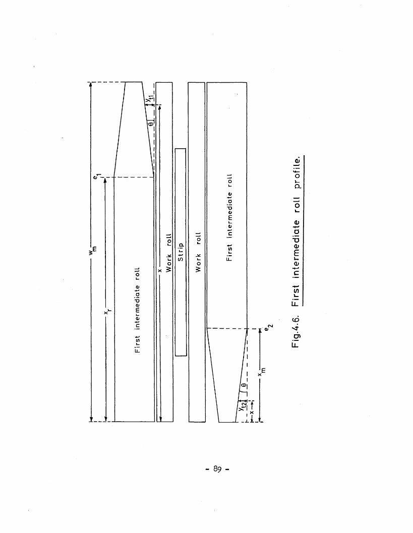
i>ri

aLi_

CM

®l

to

oi-Q.

toOioOE u.<U

•HC•*-»(/)i_lZCD

&L

- 89 -

X

(a)

Y

Fig. A.7. Forces acting on one roll in cluster.

- 90.-

BC

Fig. 4.8. Equivalent elastic foundation constant.

- 91 -

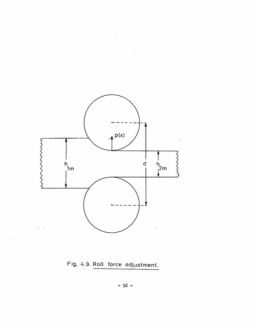
. P(X)

2 m1m

Fig. 4.9. Roll force adjustment.

- 92 -

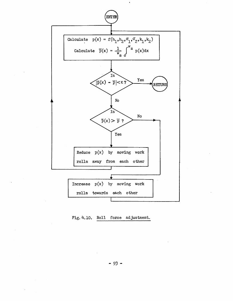
Calculate p(x) = f (h^l^^O^k^,!^)i rwCalculate p(x) = --- j s p(x)dxw J s o

1 t

RETURN

Yes

v____Reduce p(x) fcy moving workrolls away from each other

________________ iIncrease p(x) by moving work rolls towards each other

Fig. k. 10. Roll force adjustment.

ENTER

Calculate y ^ (x )

Calculate q(x) = f(y12(x))_ i fwCalculate q(x) = J q(x)dx

No

^ I s \ ^ Noq(x)> a ? /

V i e sJ!_____

Reduce <l(x) by moving the tworolls away from each other

___________________ f~Increase q(x) by moving the two

rolls towards each other

Fig. 4.11. Flow chart for roll pressure calculation(Subroutine INPRESS).

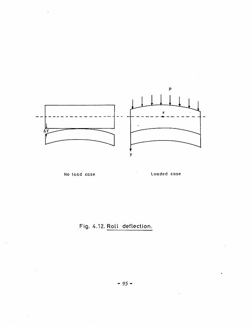
p

y

No load case Loaded case

Fig. A.12. Roll deflection.

- 95 -

F+AF

Fig. 4.13. Roll resting on an elastic foundation.

X a?

Yes

retur:

Calculate force acting on jth segment F.(x) = f(P(x),P1(x),P,(x))

and replace x by (£ - x). y, . = f(F.(x),b,a)

Fig. k.lU. Flow chart for deflection calculation(Subroutine MUMMY ).

B-N

F + d F

h + d h

d x

Fig. 4.15. Roll gap v a r ia b le s .

- 98 -

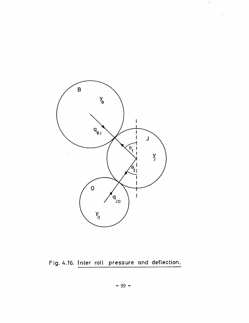
JO

ig. 4.16. Inter roll pressure and deflection.

START'

IsYes

E < ACC ?

No

Calculate yj using q^j and q ^

Calculate E = •BJNEW •BJOLDJL

-dJpdate qBJ Calculate net force acting on J

Calculate yJNQJ = fy(P) Calculate Yj = Yj - a(Yj - YJ M

Fig. k.l7. Flow chart for qBJ calculation.

- 100 -

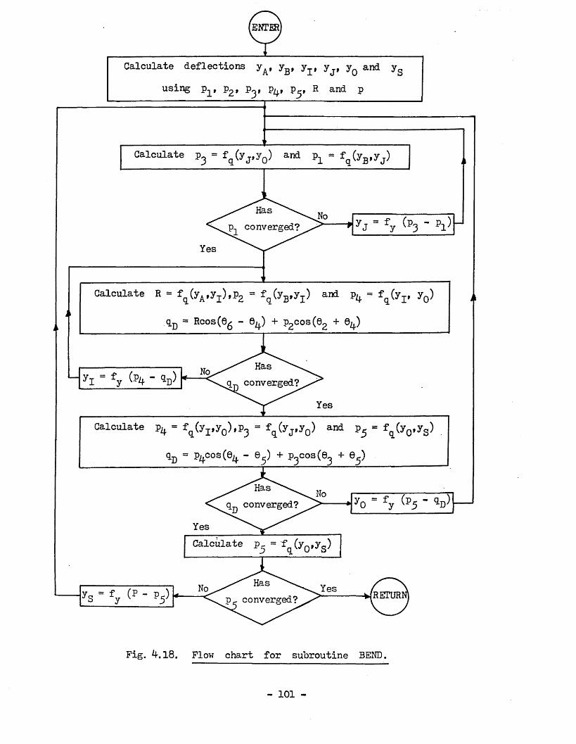
Calculate deflections yA , yB , y.^ yJf yQ and ys

using •Pi* P£» PZj.* Pjj» ® and p

Calculate ?3 = fq(yJfy0) and P;L « fq(yB,yj)

yJ = fy (p3 ' *1>

Calculate R = fq(yA,yI),P2 = fq(yB,y-[) and p^ = fq(yI( yQ)

tD = Rcos(6g - e4) + p2cos(e2 + 9^)

L yi - fy (pH - 1D)

YesCalculate p^ = fq(yI,y0),P3 = fq(yj,y0) and = fq(y0,ys)

iD = p c°s(e - ep + p3cos(e3 + e5)

yo = fy (p5 ‘ ^

Calculate = fq(y0>ys)

yS = fy (p - p5} RETUR

Fig. 18. Flow chart for subroutine BEND.

- 101 -

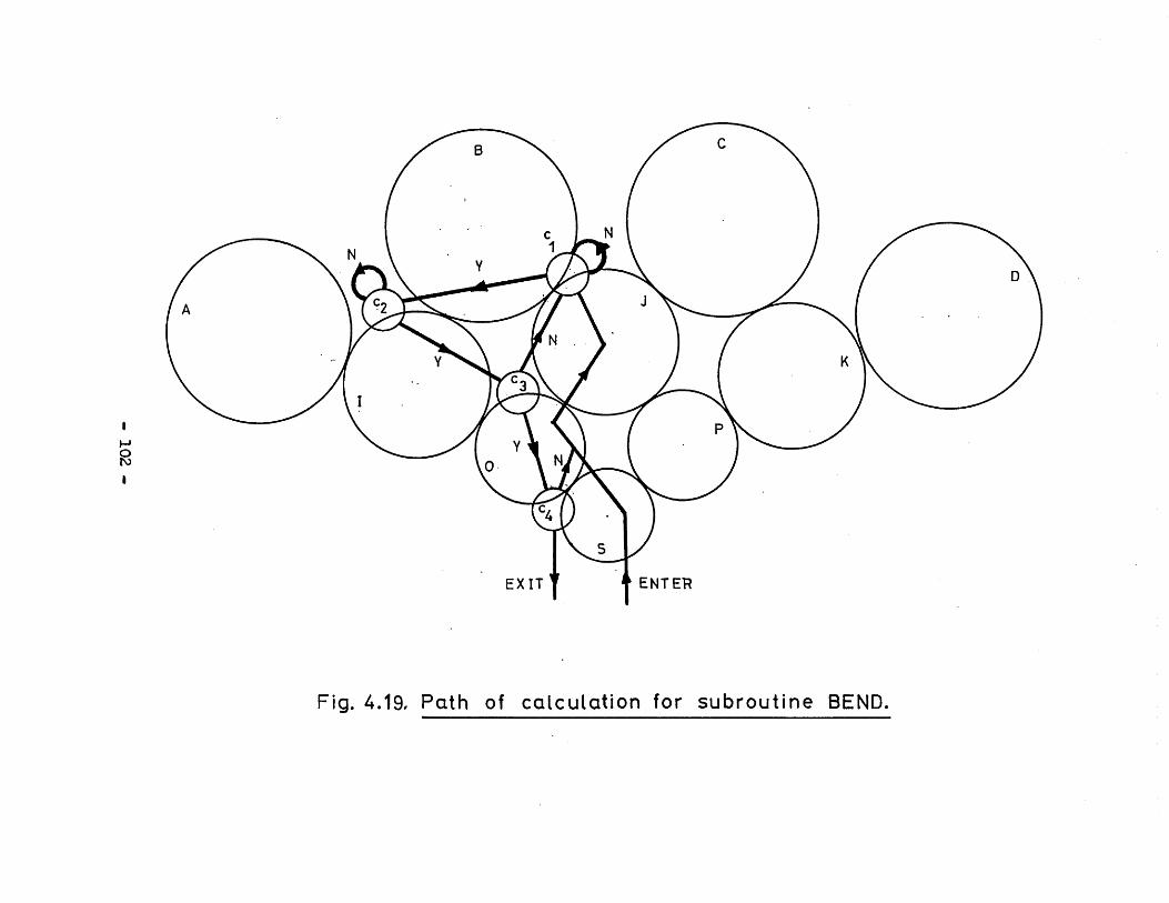
in

h-xUJ

- 102 -

Fig. 4.19, Path of calculation for subroutine BEND.

Chapter 5.

STATS SPACE REPRESENTATION OF THE MILL.

5.1. Introduction.

The analysis and design of linear systems can be achieved by using one of two major approaches. Onemethod uses Laplace and z-transforms, transfer functions, and block diagrams. The other approach, in which modern control system design techniques are based, is the statevariable technique.

The state variable method has at least thefollowing advantages over the transfer function methods

1. It is convenient for computer solutions.2. It allows a unified representation of digital

systems with various types of sampling schemes.3. It allows a unified representation of single and

multivariable systems.4. It can be applied to certain types of nonlinear

and time varying systems.

In the state variable method a continuousdata system is represented by a set of first orderdifferential equations called state equations. For a discrete system the state equations become first order difference equations?0,51

- 103 -

5.1.1. State equations for continuous systems.

The multivariable continuous system with m inputs and r outputs shown in fig. 5.1 can be characterised by the following set of n first order differential equations:

where x^(t),..*xn(t) are called state variables. The r

outputs yk(t) (k = 1,2,.. .r), can be related to the state

variables and the inputs in the following manner:

Sis. (5.1) and (5.2) can be written in compact form using vector terminology as

where A, B, G and D are constant matrices for linear timeinvariant systems.

The solution to eq. (5.3) can be obtainedusing the Laplace transform method and is given by

x(t) = Ax(t) + Bu(t) (5.3)

and

y(t) = Cx(t) + Du(t) (5 A)

§ (t - x)Bu(x)dx t^O■t

(5.5)0

-1 04-

where

-1 00

$(*) " J Z [(sl - A)_1] = eAt = / Ak-j| (5.6)k = 0

and §(t) is called the state transition matrix. Bq. (5.5) is true only when the initial time is taken at t = 0. If the initial time is taken to be t then eq. (5.5) can be

modified to include t and is written aso

f.x(t) = $ (t - tQ)x(to) + I §(t - x)Bu(x)dx t^tQ. (5.7)t o

5.1.2. State equations for discrete systems.

A discrete system is shown in fig. 5.2. The inputs to the linear system are discretised and they are described by

u^t) = u^(kT) = ei(kT). (5.8)

Now letting t = kT and since u(x) = u(kT) = constant vector,

eq.. (5.5) for discrete system can be written as

-tx(t) = $(t - kT)x(kT) + I$ (t - x )Bdx

kTu(KT). (5.9)

Bq. (5.9) is only valid for one sampling period. If we are interested only in the response at the sampling instants by setting t = (k + l)T we obtain the discrete version of

- 105 -

(5.10)

(5.U)

(5.12)

5.2. Mill representation in state space form.

5.2.1. Introduction.

The overall block diagram of the shape controlscheme is shown in fig. 5.3• The control scheme is divided into several subsystems. The system has 8 + 2 inputs and anumber of shapemeter measurements (^31) as outputs. The 8 + 2 inputs represent eight As-U-Roll actuators plus thetwo first intermediate roll positions. For the present analysis it is not proposed to control the first intermediate roll positions. Therefore only the eight actuators are considered as inputs. The investigation becomeseasier when the number of inputs are equal to the number of outputs, hence for the initial design it is assumed that there are eight shapemeter outputs. This is done by dividing the strip into eight zones and treating shape at each zone as constant.

eq. (5.5) as

x[(k + 1)T] = $(T)x(kT) + A (T)u(kT)

where

§(T) = eAT

and

A(T)= f §[(k + l)T-t]J n

Bdl

- 106 -

The set point actuators are assumed to controltheir positions by means of a servo type control system.Variations in the actuator positions are assumed to have aninstantaneous additive effect to incoming shape. This isjustified, as the dynamics of the mill cluster are muchfaster than the overall system dynamics and can be ignored.A movement in any one actuator affects the shape acrossthe entire strip width. Any corrective effect of the shapeat the roll gap due to actuator movement is calculated

39from the static mill gains. These effects are added to the incoming strip shape disturbance. The shapemeter is situated at a fair distance from the roll gap and therefore the stress distribution of the strip, as it movesdownstream to the shapemeter, is affected by a combinationof pure transport delay and a lag effect. The shapemeter transducer is effectively a discrete system, as explained insection 2.3.2, the output from it being electronically smoothed by filters.

52A cascade controller is proposed to correctshape changes and the control is obtained by comparing theshapemeter measurements with the actuator signals whichproduces zero shape.

5.2.2. The actuator subsystem.

The eight actuator's are assumed to benoninteracting and are modelled as second order systems. Inpractice actuators are simple integrators accompanied by a

- 107 -

dead space arising from the solenoid valve spool, and from friction in the hydraulic motor. The open loop transfer

The output position can he fed hack via a position tranducer to control the actuator positions accurately. The forward path has a variable gain k and the closed loop system for one actuator is shown in fig. 5. . The closed loop transfer function of the actuator can he written as

of eq. (5.1^0 are complex then the actuator positions will have overshoots. Since the mill dynamics are much faster than the overall system dynamics, these overshoots have instantaneous effect on shape which will cause a problem on control. Therefore it is proposed to choose k to give equal roots for the characteristic equation so that the actuators will have the fastest response without any overshoot. Hence the closed loop transfer function of each actuator can he written as

function for the actuators can he written as'52

Ga(s) s(l + sT ) ‘EL

(5.13)

sa ^ s(l + sT ) + kk k„ - N a' a fkka (5.14)

3f the roots of the characteristic equation

(5.15)

- 108 -

The state space form of each actuator is therefore given by

= V i a M + Baua (t)CL CL CL CL CL

= 0A ( t )(5.i6)

where

1i —101

~ '

A = ' Ba =CL

1 2CL

kay k

11

and Ca = [l 0] (5.17)

(See Appendix 3 for numerical values of and T^). Since

there are eight actuators with eight inputs and eight outputs, and they have the same transfer function, the state space form of the multivariable nature actuator subsystem can be written as

l i W [/

U b W .

al 0

0 a8

Bal 0

0 Ba8

and

G ,al 0 0 •

0 • •

5al<tJ iv. 0 • •• •• •• •« #0

. ° ’Ca§ra8l0 0

0 00 -i X_o(t)-a8(5.18)

- 109 -

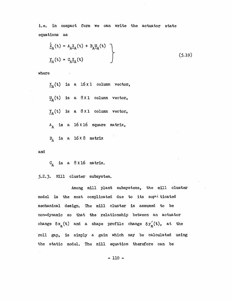
i.e. in compact form He can write the actuator state equations as

= aa ^ a W + ba2a W 1I (5.19)

rA(t) = cAxA(t) J

where

xA(t) is a 16 X 1 column vector,

is a 8X1 column vector,

is a 8X1 column vector,

Aa is a 16 X 16 square matrix,

ba is a 16 X 8 matrix

CA is a 8 X16 matrix.

5.2.3. Mill cluster subsystem.

Among mill plant subsystems, the mill clustermodel is the most complicated due to its so^i ticatedmechanical design. The mill cluster is assumed to benon-dynamic so that the relationship between an actuatorchange 6x (t) and a shape profile change 5y/(t), at thea mroll gap, is simply a gain which may be calculated usingthe static model. The mill equation therefore can be

- 110 -

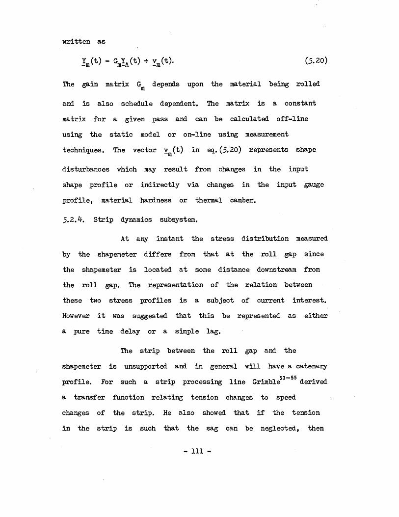
written as

i W - W * ) + I.W- ^-2°)

The gain matrix G^ depends upon the material being rolled

and is also schedule dependent. Ihe matrix is a constantmatrix for a given pass and can be calculated off-lineusing the static model or on-line using measurement techniques. The vector Y (t) in eq. (5.20) represents shape

disturbances which may result from changes in the input shape profile or indirectly via changes in the input gauge profile, material hardness or thermal camber.

5.2. f. Strip dynamics subsystem.

At any instant the stress distribution measuredby the shapemeter differs from that at the roll gap sincethe shapemeter is located at some distance downstream from the roll gap. The representation of the relation betweenthese two stress profiles is a subject of current interest. However it was suggested that this be represented as eithera pure time delay or a simple lag.

The strip between the roll gap and the shapemeter is unsupported and in general will have a catenary

5 3 —55profile. For such a strip processing line Grimble deriveda transfer function relating tension changes to speed changes of the strip. He also showed that if the tension in the strip is such that the sag can be neglected, then

- Ill -

the transfer function can be represented by a simple lag term. Since the stress at the roll gap depends on the input/output strip velocities it can easily be shown thatthe relationship between the shape at the roll gap and the

52shape at the shapemeter is also a simple lag term. The shapemeter is situated at a certain distance from the roll gap, and therefore the shape measured at the shapemeter is not the true shape, but delayed by time x. Thus for the present analysis the transfer function of the strip includes a time delay term and a simple lag term in cascade. Therefore the transfer function of the strip is written as

•■STFor simulation purposes the delay term e is replaced by first order Fade approximation and hence the strip transfer function is given by

The state space form of one of the strip zones is given by

(5.22)

- 112 -

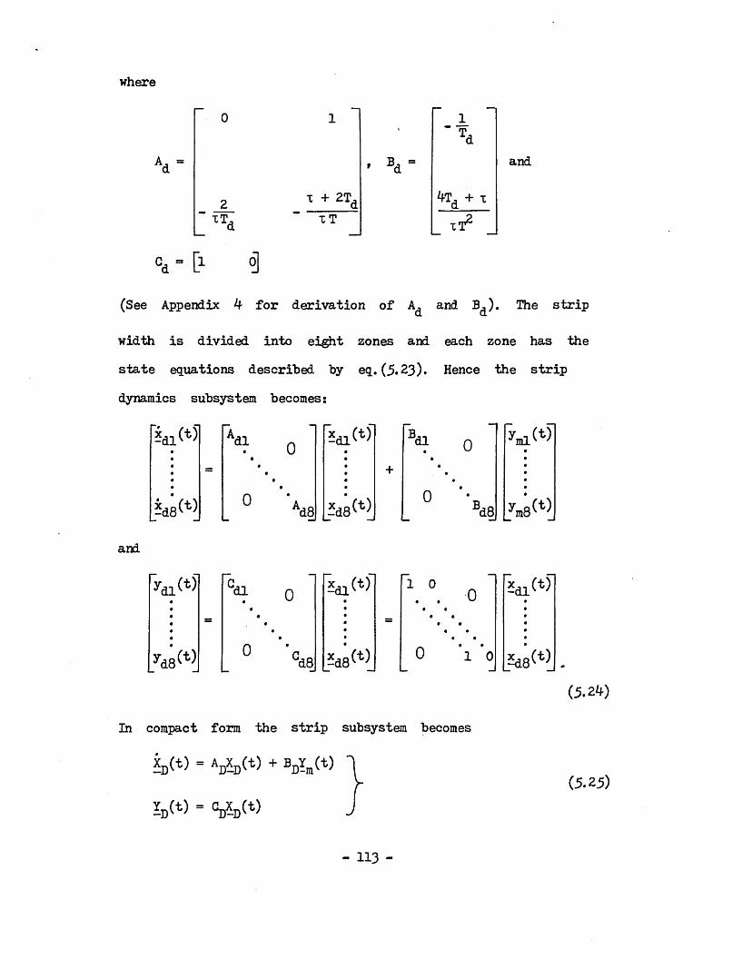
where

0 1 -

1 .

rH 16- 1

1

Ad = • Bd =

2 x + 2Td tod + xXT 1R1

and

cd = C1 o]

(See Appendix U for derivation of and B^). The strip

width is divided into eight zones and each zone has the state equations described by eq. (5.23). Hence the strip dynamics subsystem becomes:

*41(*J

SaaW

(11

0

0

<18

Bdi ot

0 Bd8

"y» l W

and

’ydi^>••••••

yd8^t}_ —

“dl

0

0 5 a i W

3) _^d8(t)_

l o0« •

# •• •

• •• •

• •• •0 1 0

i a i M

(5.2*0In compact form the strip subsystem becomes

& (*> - W * ) +

V * ) "

(5.25)

- 113 -

ifech strip zone is second order and therefore eq.(5.25) has the dimensions as eq. (5.19).

5.2.5. The shaperneter dynamics subsystem.

is represented by a second order system with a dominant shapemeter filter time constant which varies as the strip speed (see Appendix 5). A series of filters is switched on at preset mill speeds to smooth the discretised shapemeter signals. The shapemeter signals from the thirty one measuring zones are assumed to be non-interactive and are reduced to eight signals to avoid dimensionality problems. The shapemeter transfer function approximates to a unity gain second order system and is given by

where Tg^ is the speed dependent dominant time constant. In

state space form the shapemeter is represented as

The shapemeter forms an output subsystem and

1 (5.26)(1 + sTsl)(l + sTs2)

(5.27)J

where

The complete shapemeter subsystem consists of eight zones and hence this subsystem is represented in state space form as

2s8(t).

si 0

o \•••

•+

3J•

2s8W

Bsi

0

0

Bs8

and

ys l W••«•••

Ja8(t>

si

0

0

-s8

2 s l ^

2s8 W

1 0 0• •• •

• •• •• •

# #• •o l o

yd l(t)

yd 8 ^

*sl(t)

*38^(5.28)

In vector form the shapemeter subsystem becomes

Xs(t) - AgXs(t) + BgYjj(t)

Ys(t) = CsXs(t).(5.29)

Since each zone is second order eq. (5.29) has the same dimensions as eq.(5.19)*

5.3, State equation of the complete system.

Efts. (5.19). (5.20), (5.25) and (5.29) can be combined, to represent the complete multivariable system in state space form, as follows:

YA(t) is substituted from eq. (5.19) in eq. (5.20) to give]L(t) - 5 C X ( t ) + Vm(t). (5.30)

- 115 “

Bj. (5.30) is substituted in eq. (5.25) to give

y * ) = w * ) + 4 V A W +

- w Ay * > + w * > + y y ) • (5.31)

From eq. (5.29) YrjC ) *s eliroi^ted using eq. (5.25) to give

y * ) - + * * < * 5 • (5.32)

The state equations of the complete system in terms of subsystems can be written as

XA(t) = AAxA(t) + BAuA(t),

y *> = w a w + w + •

Xs(t) = BgCjjXjj(t) + AsXs(t),(5.33)

Ig(t) ^

Hie set of eq. (5.33) can be put in the matrix form as

X(t) = AX(t) + BU(t) + Dym(t),

Y(t) = CX(t)

where

(5.3*0

B_G C.D m A

*3%

( W x M ) (5.35)

- 116 -

'ba

B = 0

0 _

"o'

» (48 X 8) (5.36)

D = bd _0 .

t (48 X 8) (5.37)

G = [° ^ Cs], (8 X 48) (5.38)

XT(t) =1j£(t) *£(*) Xg(t)]. (5.39)

uT(t)= 1~ua l W ........ “a S ^ ’ (5.40)

yT(t) -[/s l(t) W * ) ........ (5.41)

This state space description of the mill forms the basis of the dynamic model simulation. In the above description the A matrix being lower triangular allows some simplifications in the computation. For control design the transfer function form of the system is more convenient.Also the plant structure is indicated far more clearly than in the time domain equations. As explained in section 5.2 all the dynamic elements are non-interactive. Therefore the actuator, strip and shapemeter subsystems can be written respectively in matrix form as

K,G (s) = ---- £

(1 + sT.)2 I 8 (5.42)

(5.43)

and

(5.44)

where Ig is the 8x 8 identity matrix.

Therefore the open loop transfer function matrix G(s) of the system can he obtained as

where N(s) and D(s) are numerator and denominator polynomials respectively. (See Appendix 6 for polynomials N(s) and D(s) obtained for low, medium and high speeds).

5 A. Shape profile parameterisation.

profile presents several advantages and is often used. In the present system the maximum number of shapemeter outputs to be controlled are thirty one. The number of shape outputs also varies with the strip width. It is convenient if the number of outputs to be controlled is fixed for design purposes. Since the shape profile is a smooth curve

G(s) - Gs(s)Gd(s)G]liGa(s)

Ka(1 - st/2)(1 + sTa)2(1 + st/2)(1 + sTd)(l + sTsl)(l + sTs2) m

(5.45)

The use of parameterisation of the shape

- 118 -

this can be represented by a polynomial of given order. If the parameters of this polynomial are taken as outputs then the number of outputs to be controlled become fixed ratherthan controlling the shape outputs directly. If the shape profile is represented by a third order polynomial (say

ax*' + bx + cx + d) then the number of parameters to be controlled become four namely a, b, c and d. This means that parameterisation reduces the number of outputs to be controlled.

Let y (x) be the shape measured or observed sat the shapemeter and x be the distance across the strip width. The measured shape can be expressed in matrix formas

Y(x) = xp + e (5.46)

where p is a vector containing the parameters to be controlled, £ is a vector of errors and X is a known constant matrix. If the polynomial which describes shape is third order then

pT - [a b o d], (5.47)

The error sum of squares is

eTe = (Y - Xp)T(Y - Xp)

= yty - 2pTxTy + pTxTxp . (5.48)ALet p be the least square estimates of p which when

Tsubstituted in eq. (5. +8) minimises ee. This can be obtainedby differentiating eq. (5.^8) with respect to p and equating

representing the shape are taken as the outputs of thecontrol system. A modified block diagram of the shapecontrol system is shown in fig. 5.5. In this figure G(s) represents the transfer function matrix of the plant and is given by eq. (5. 5). There are eight actuator input signals to this block and the outputs are the eight shapemeter measurements. These eight signals are transformed into fourestimated parameter outputs using eq.(5.^9). These four estimated parameters are compared with four reference parameters (r to r^) which will produce the desired shape.

The controller is a tyx k matrix which transforms these error signals to control signals u(t). These four control inputs must be transformed via a matrix to act on theplant matrix G(s). This transformation matrix may be chosen freely. However, if same matrix X is selected, as shown in fig.5.5f the open loop transfer function becomes

the result to zero. This will give a solution to p as56

A T 1 Tp = (xAx) •LxJ,y ..Tv N-1vT, (5.49)

Thus the estimated values of the parameters

Gx(s) = (XTX)"1XTG(s)X

(5.50)

- 1 20 -

where G ^ = (X^X)"^X^G X and G^(s) will be a matrix.

5.5. Shape control system design.

An acceptable control scheme must provide:1. Transient response with small overshoot and rise

time in the region of say 5 seconds (experience of mill operators).

2. Relative insensitivity to errors of calculation andvariations of static gain matrix G .m

3. Relative insensitivity to line speed.

Furthermore there are certain shape profiles which must never be reached, even in transients, for the safe operation of the mill. These aspects are still under discussion with the mill engineers.

As discussed in section 5.2 the mill is amultivariable plant with eight inputs and eight outputs. Straight forward application of either of the two modern

57multivariable design methods, i.e. the Characteristic Locus58or the Inverse Nyquist Array, will produce compensators

highly dependent on G~^ as all the interactions in the

plant comes from G . From the properties of G describedm mby eqs.(6.l) and (6.2) in section 6.1, the matrix G^ is not

of full rank and therefore the inverse does not exist. But the matrix G , calculated from the static model described

- 121 -

in chapters 2 and 3» is often full rank and this may bedue to numerical errors. Consequently a control systemcannot be based on G~\m

The use of input-output transformation of theplant discussed in section 5.^ produces a smaller dimensionsystem. This yields a four by four multivariable system with Gx(s) as the forward path transfer function (eq. (5.50)).The gain matrix G ^ in eq. (5.50) is not diagonal. Suitable

pre and post compensators can be found to diagonalise G ^

using singular value decomposition to reduce interactions.

5.5.1. Singular value decomposition.

The singular value decomposition was developedfor real square matrices in the 1870's by Beltrami andJordan?9 The singular value decomposition theorem60 can be stated as, 'If A is a real nxn square matrix then there exists orthogonal real square matrices U and V such that

A = USVT (5.51)

whereS = diag(olf 02, on) (5.52)

Proofs-TSince A A is symmetric and positive definite

Tthe characteristic roots or eigenvalues of A A are real and positive. Denoting these characteristic roots by

i = 1, 2,.......n

we can arrange that

o - j (5.53)

Let v^f v^f....vn be the corresponding orthogonal

characteristic vectors, i.e. V = (v.,, vot..... v ) is' 1 c. northogonal. If

S = diag(<rlf 02,.... 0n) (5.5*0

and

S2 = diag(o2, .....a2) (5.55)

then we have

ATAV = VS? (5.56)TSince V is orthogonal V V = I and eq. (5.56) can be written

as

s“1vtatavs“1 = s"1vTvsss"1 = I . (5.57)

Let

U = AV3"1. (5.58)

- 123 -

Therefore

UT = S ' V W (5.59)

Then from eq. (5.57) we have

UTU = I (5.6o)

which means that U is orthogonal. Then from eq. (5.57) we have

U'*’A VS*"1 = I (5.61)

from which

A = USVT. (5.62)

Prom the above theorem, the transformed gainmatrix G can be written as mx

Gnx = U I V T (5.63)

where I is a diagonal matrix, and U and V are orthogonal matrices. Prom eq.(5.63)

utg v = I . (5.64)mxTIf V and U are chosen61 to be the pre and

post compensators, the forward transfer function of the plant can be written as

F G P, = Mf2.UTG V 1 x 2 D(s) mx

= 5 ^D(s)

I (5.65)

- 124 -

and the closed loop transfer function matrix becomes-1

Gci/S)- N(s)D(s)

•I- + W(b )D(s)

(5.66)

The present study is only concerned with thestatic model and therefore the actual control system designis not discussed any further. The results for singula valuedecomposition are given in chapter 6 and the complete blockdiagram for the plant is shown in fig. 5.5.

- 125 -

U1(t)------------►u 2( t ) ----------- ►

u m < t ) ---------------------------- ►

Sta te variables

yn ct)

-► y 2( t )

-► y r ( t )

Fig. 5.1. M u lt iva r iab le linear continous system.

>y(t)e ( t )

* y ( t )

Z.O.H.

State variables

Fig. 5.2. Multivariable linear discrete system.

- 126 -

X *D CL Q. Oo w

cn>tn

* uE E0> oQ. cO

SZ *D

r 00

(/)cn

“T

I 1I -IU),| cn I

y>■ 1

CDt/>cn

00

.9*6 r ~ •— i 1-1 CO"D X>, "D

m | cn 1 cnL « J

co a><u u

-W-+X 1

r-o_ • ‘-i ood i ° dcn 'cn 1 cn

L.J

EdL_cnOx>oo

o>ocoLOg>u_

- 127 -

Forw

ard

Act

uato

r tr

ansf

erinoa.

*o

E<DI/)>*I/)

Coac oI/)oCl

d3ud

E ocndTJ

ooCD

LOdi

Ll

- 128 -

CO

00

X

f-XXX

oh-

E<DWcn

c o<J

)CLa_ccn

£d»_cnd"Ou

_oCD

LOinCTL

- 129 -

Chapter 6.

RESULTS AND DISCUSSION OF RESULTS.

6.1. Properties of shape profiles.

The static model provides two main types ofresult for a given rolling schedule. The first category is concerned with the physical processes and is the calculated shape, gauge and pressure profiles. These are important when the degree of control of a particularprofile is of interest. The shape profiles for eightactuator changes (RUN 0) are shown in fig. 6.1 (e.g. infig. 6. la the curve marked with a cross is the shape profile due to a change of 6 mm in rack 8, keeping all other racks at zero position etc.). Inspection of figs. 6.1 to 6.22 shows the property of symmetry when the strip is placed at the centre of the mill. Units used in these figures are N/m for shape and the distance x is given in terms of number of sections. The actual distancecan be obtained by multiplying the number of sections by dx the width of one section. Inter roll pressure distributions and the corresponding roll deflections for a change in rack 1 are shown in fig. 6.2^ and fig. 6.25

respectively. These profiles are obtained for the mill schedule given in table 6.1. The corresponding gain matrix is denoted by G ." m

- 130 -

If the shape profiles shown in fig. 6.1 are inspected closely it is seen that the largest shape changeis found in the vicinity of a point, which is directly under the particular shape actuator which has been moved from the null point, across the strip width. It is also clear that a rack change appears to affect widely separated sections of the strip. This can be explained by considering a localised change in the back-up rolls. This change in the back-up rolls will modify the inter roll forces between the back-up and second intermediate rolls. Similarly, this change in the inter roll force will change the effective profiles of both the back-up and second intermediate rolls. From the study of a point force acting on a roll, it can be seen that the roll profile is changed, not just below the point of action of the force but over a regionsurrounding the point. The change is significant in the vicinity of the point of application of the force. Thus, a localised change in the back-up roll profile is converted to a distributed change in the profile of the second intermediate roll. Further interaction between the second intermediate rolls and the first intermediate rolls and between the first intermediate rolls and work rolls spread the effect. Thus in general the largest shape change occurs under the actuator which is moved.

In fig.6.1 the negative shape corresponds tocompressive stresses and the positive shape to tensile

- 131 -

stresses. When rack 1 is moved downwards for example, the left hand side of all the rolls will be deflecteddownwards with respect to the other end. This results in an increase in reduction of the thickness at the left hand edge of the strip which will produce a longer edge.To keep the applied tension constant, the left hand edgeof the strip must be compressed and at the same time the right hand end will have tensile forces. This corresponds to the compressive and tensile nature of the stress and is shown in fig. 6. la.

*■' The static model developed ignores the strip edge effects. When the strip width is less than the millwidth (or the length of the work rolls) there will be two portions from either end of the upper work roll withno support. The model is based on the assumption of zero shape directly under these two portions and therefore the shape changes from zero to a high value at the edge ofthe strip. This is shown in fig. 6.1 (and in all other shape profiles where the strip width is less than the mill width) by the rapid change at the edges. The calculated shape near the edge of the strip is therefore not the true shape.

6.2. Properties of the mill gain matrix.

The mill gains represent the second majorsource of information available from the static model.

- 132 -

Linearised mill gains are calculated about a given shapeoperating point and these relate the shape changes to theAs-U-Roll changes. If the shape is measured at eight zonesacross the strip, the gain matrix has the form G^ givenin section 6.6 (units = N/mm^). The eight rows of thegain matrix represent the eight zones across the stripand the eight columns correspond to eight As-U-Rolls, e.g.the elements in the second column give the shape at eachzone across the strip width when the second As-U-Roll is moved. Thus, g ^ = -0.377 in G^ is the shape at zone 4- when As-U-Roll 6 is moved. The negative gains result fromthe assumption that the average tension is maintainedconstant. The gains include small errors due to numerical problems and due to the fact that the mill is non-linear. The gains are dependent upon the operating point and arevery dependent. upon the strip width. The way the gainmatrices vary with different schedule settings are shownin table 6.3.

If the strip is centred across the mill thenthe gain matrix has a special type of symmetry. The firstfour columns of the matrix are repeated as the last fourcolumns but in reverse order and vice versa. Anotherproperty of the gain matrix is that the elements of eachcolumn and row sum to zero. That is, it must satisfy

- 1 33 -

8 ^

2 Z eij = 0 . (6,1)3 = 1

and

8g. . = 0 .

Z_ , e i 3i = 1

Eg. (6.1) describes the condition that the row elements sum to zero. This can be explained by consideringa situation where all actuators are moved together by the same amount. This would result in a movement of the work rolls vertically downwards without introducing any bending effects, which is equivalent to a screwdown movement situatedat the sides of the mill. The resulting major effect willbe on the strip thickness and there will be no appreciableshape change. This is the case for RUN 22 and fig. 6.23shows the corresponding shape profile which illustrates this point clearly,

Bg.(6.2) is the condition that the columnelements sum to zero. This is so since by the definitionof shape (the deviation in the tensile stress from themean), the average value across the strip should be zero.

Table 6.3 is obtained by comparing matrices

G^ to G ^ with G . The diagonal elements are compared andm m mthe changes are expressed as a percentage change. The

(6.2)

- 1 3 ^ -

negative sign indicates a reduction in gain compared to

and the overall, change is the average percentage change when all actuators are considered.

6.3. Shape changes for strip width variation.

1 7The gain matrices G to G given in sectionm m6.6 are obtained by varying the strip width from 1.7m to1.0m and keeping all other variables constant. The corresponding shape profiles are shown in figs. 6.1 to 6.7.All these shape profiles and gain matrices have theproperties discussed in sections 6.1 and 6.2 if minor numerical errors are ignored.

The maximum shape occurs in the vicinity ofthe particular actuator which has been moved. In figs.6.1to 6 .8 this is shown as the minimum or the trough of theshape profiles. A graphical representation of the variation of these maximum values is shown in fig. 6.26. As seen from the figure the maximum shape hardly changes with the strip width if actuators 3» 5 and 6 are used. This is becauseall actuators are situated well within the strip considered. The distance between racks 3 and 6 is about 0.68m and theminimum width considered is 1.0m. Therefore racks 3t 5and 6 lie well within the strip widths considered. When there is any change occurring in these four lacks, there isa portion of the strip directly under the particular rackmoved to support the work roll. For these widths the

- 135 -

conditions of the strip in the vicinity of racks 3» 5

and 6 do not change considerably, and hence the shapechange due to the same movement in any of these four rackswill be roughly the same (see figs. 6.1 to 6.8).

The maximum shape for strip widths 1.7m and1.6m remain approximately the same when racks 2 and 7 are used. This is similar to the above case as racks 2. and 7 are situated well within these two strip widths. If thestrip width w is reduced further then the work rolls have nosstrip to support and they act as cantilevers. This cantileverbending action will attempt to reduce the thickness of thestrip at the edges more than at the middle and thereforewill produce higher compressive stresses near the edge. Thelength of this cantilever portion increases when w issreduced, and hence the bending action which produces thevariation in the maximum shape. As seen from fig. 6.26, thevariation of maximum shape for racks 1 and 8 has amaximum (in the negative sense) when w = 1.5®, and forsracks 2 and 7 this occurs at w = 1.4m. When w iss sfurther reduced than these two limiting values, the twowork rolls will touch each other. This reduces thecantilever bending effects on the strip edge and thereforeresults in a reduction of the magnitude of the maximumshape.

- 136 -

The corresponding gain matrices for the seven1 7different widths are denoted by G to G in section 6.6.m m

It is seen from these matrices that the gain elementsreduce in magnitude as w decreases. In table 6.3 thesfirst seven rows represent the percentage change in diagonal

1 7 0elements of G to G compared with G which is the gainm m mmatrix when w = 1.4m. The details of RUN numbers are given sin table 6.2. The overall percent change is the averagechange in diagonal elements. This overall percent change isjust an indication showing how the gain matrices varycompared to G°. RUNS 1 to 3 have widths wider than for mRUN 0 (w = l.Jfia) while RUNS k to 7 have narrower widths,sIt is seen from table 6.3 that the overall percent changedecreases with w .s

When using narrower widths the region of workroll which is in contact with the strip is less and thereforethe roll force p(x) must be larger to keep the force balance in the mill cluster. The interference between strip and work roll must be higher for larger roll force and hence the output thickness becomes smaller, j rom eq.(3.13) it is seen that the output stress is smaller for smalleroutput thicknesses and hence the gains must decrease withthe strip width.

- 137 -

6.4-. The effect on gains of changing other variables.

In the previous section the effect of theg

variation of strip width was discussed. The matrices Gm22to Gm axe the gains of the mill for the cases in which

the strip width is fixed at w = 1.4m. All these casesshave the mill schedule used for RUN 0 (see table 6.1)with one change in at least one of the input data, "thesecases will be discussed here.

The test for RUN 8 is to see the effect onyield stress of the material being rolled. The yield stresscurve (see Appendix 7) is increased by a factor of 0.5 so that the material rolled is stiffer. It is seen from table6.3 that the overall gain is reduced by 7$ for this case. When rolling harder materials the rolling force must be greater to obtain the same reduction. Higher rolling forcesproduce more interference between strip and work roll, and hence the change in output thickness will be more. This results in a smaller output stress profile and thereforethis case will have smaller gains.

The RUNS 9 and 10 are carried out to seethe effect of changing the mean reduction. For RUN 9 ihe input mean thickness is increased by 2.5 times to 6mm witha reduction of 20$ compared to 15$ for RUN 0. For RUN 10the mean input thickness is adjusted to 1.5m with areduction of 13$. That is, for the first case the reduction

- 138 -

is increased by 5$ and for the second case this is reducedby about 2$ which is roughly half the value of theprevious case. When the overall gain change figures are inspected it is seen that for case one it is -40$ andfor the second case it is about +21$, which is roughlyhalf of the previous figure. From these two results it isseen that the gains of the mill obey approximately alinear relationship with the percentage reduction.

The RUNS 11 to 16 correspond to changes in roll diameters. RUNS 11 to 12 show the effect of workroll diameters, RUNS 13 to 14- the effect of firstintermediate roll diameters and finally RUNS 15 to 16 theeffect of second intermediate roll diameters. In each case the diameters are changed by + 15$ and the changes of the overall gain are given in table 6.3. When the work rolldiameter is reduced the overall change in gain is + 7.9$ and this figure is -6.7$ for the bigger work roll. For the first and second intermediate rolls these figures are + 2.3$ and - 2.8$, and + 8.8$ and - 8.0$ respectively. When the diameter of a roll is increased the deflection caused by a given mill loading will decrease, that is, the roll will become stiffer. In other words, the bending effects will decrease. When the roll diameters are changed by the same amount ( + 15$) the figures show that the correspondingchanges in gain also have the same order of magnitude, except for the case of the first intermediate roll. This may

- 1 3 9 -

be due to the fact that the first intermediate rolls arefurnished with tapered ends, which will produce a lessbending effect than a roll without tapered ends. The function of first and second intermediate rolls and back-up rolls is to prevent excessive bending of the work rollswhich assist the elimination of shape and gauge defects.Also the roll separating force for a given reduction increases with roll radius. The effect of increasing roll diameters is therefore to increase the roll force which inturn reduces the gains of the mill. Conversely if smallerrolls are used the corresponding gains will (<3 crease}

For RUN 17 the mill cluster angles 0^ to

are changed as given in table 6.2. For this RUN theoverall gain is increased by 9.8$. The change in clusterangles will disturb the mill cluster configuration and the vertical and horizontal components of roll separating forces will therefore differ. This will change the roll force and hence the change in gain follows.

The RUNS 18 and 19 show the effect ofchanging the output tensile force. In RUN 18 the tension is decreased by 50$ to 95294-N and for RUN 19 it isincreased to 285882N again by 50$. The overall gain changefigure for these two cases are +2.4$ and - 3.1$ respectively. When rolling metal strips higher reductions or smaller output thicknesses can be obtained for higher output tensions, assuming that the roll force remains the same.

- 1 40 -

Smaller output thicknesses mean smaller stress profiles and hence mill gains will be smaller for higher tensions.

The first intermediate rolls are moved by 100mm for RUN 20, and there is an increase of 6. Z% in the overall gains of the mill. The edges of thetapered wedge positions (vertical planes e^ and e^ in

fig.^.6 ) of the first intermediate rolls are set at the vertical plane passing through the strip edges for RUN 0.That is, along the strip width, first intermediate rolls havea flat surface. This is not the case for RUN 20, wherethese rolls are pushed in by 100mm, so that the roll surface is no longer flat. That is, near the strip edgearea first intermediate rolls have a smaller diameter. This increases the bending effect of this roll thus increasingthe gain.

RUN 21 is carried out to see the effect ofincrease in the roll rack movement. Here all racks aremoved, individually one at a time, by twice the distance as

0 21for RUN 0. If each element of gain matrices G and ism mcompared it is seen that the change is quite small. Theoverall gain changes by +0.3$ an& theoretically these twomatrices must be the same. The variation is due to numerical errors.

RUN 22 is a special case where no comparisonis made with matrix G . This is to see the effect ofm

- l 4 l -

moving all racks at the same time by 6mm. As seen from22the gain matrix all elements are very small compared

to other cases considered. The shape profile for this caseis shown in fig. 6.23 and the variation is hardly noticable. The effect of moving all racks by the same amount is tomove the whole of the back-up roll vertically. This willnot produce an appreciable change in the shape profile asthe incoming strip profile is rectangular, and there will be no transverse variations in the reduction. Hie same effectcan be produced by moving the two side screwdowns by the same amount and hence the very small gain matrix results *

6.5. Shape control system diagonalisation using singular value decomposition.

One of the most important results obtained from the static model is the mill gain matrix which is a square 8X8 matrix. £hch column of this matrix represents theshape at eight zones of the strip due to each rack movement. The overall mill block diagram is shown in fig. 5*3 and is an eighth order multivariable system and the only interaction comes ftom the mill gain matrix. It is convenient to represent the shape profile by a third order polynomial and to control the polynomial coefficients, rather than controlling the shape at eight zones directly (see section 5.^). By using a transformation matrix (see Appendix 8) it is possible to transform the eighth order

- I* f2 -

system into a fourth order system as explained in section5 A. The block diagram of the transformed system is shownin fig. 5.5. Here G(s) is the transfer function matrix ofthe plant and is given by eq. (5 A 5 )» As seen from thisequation G(s) contains the static mill gain matrix Gm andtherefore will be interactive. The transformed planttransfer function G^(s) is given by eq. (5.50), whichcontains G = (X x T V g X.mx ' m

£hch transfer matrix for all twenty one RUNSconsidered are computed and presented in section 6.6 as•Transformed gain matrix G *. A quick glance at thesemxreduced order matrices show that they are non-diagonalmatrices. To design controls it is convenient if the systemcan be made diagonal by removing interactions. The singularvalue decomposition is used for this purpose and theorthogonal matrices U and V together with the diagonalmatrix are computed. The diagonal form is obtained by

Tcomputing I = U G V for each case. In section 6.6 themxdiagonal elements of X are presented under the heading•Transpose of W vector is*, and matrices U and V directlyunder these elements. The pre and post compensators can be

Tchosen as V and U which are pure gain terms and can be implemented easily.

If these sets of U and V (for different schedules considered) are compared, it is seen that the

- 1^ 3 -

variation is quite small and they are remarkably similar. This is • encouraging as it is possible to use one set of U and V instead of one set for each schedule. This set of U and V can be derived, for example, by taking the average of each element. This has to be investigated further. By doing this of course the interactions cannot be removed completely, but can be made small so that they can be ignored. Again this area has to be investigated further by considering more mill schedules.

- l^f -

MILL DATA-.Back-up-roll diameter = 0.405 mSecond intermediate roll diameter = 0.235 mFirst intermediate roll diameter = 0.137 mWork roll diameter = 0.09 mWork roll crown(camber) = 0.0508 mmSecond intermediate roll crown(camber) = 0.0762 mmFirst intermediate roll tapered end gradient = 1 mm/mLength of tapered end = 0.355 mMill cluster angles (see fig. 2 A) 0^ = 4l.69

e2 = 3.72°e3 = 22.56°

= 6o.54° = 41.04°

06 = 79.59STRIP DATA.Strip width = 1.4 mInput mean thickness = 2.4 mmOutput mean thickness = 2.05 imiPercentage reduction = 15 %Input mean tension = 134352.0 NOutput mean tension = 190588.0 NInput mean stress = 55.98 MN/m

2Output mean stress = 92.9699 MN/mCoefficient of friction between strip and work roll = 0.06 Incoming strip is rectangular. The tapered first intermediate roll is set up so that the end of wedge is in line with the edge of strip.

Table 6.1. Mill schedule for gain matrix G^ (RUN 0).

- 145 -

RUN 1 to RUN 7 infect of changing the strip width.

RUN 1 Strip width = 1.7 mRUN 2 s- Strip width = 1.6 mRUN 3 Strip width = 1.5 mRUN 4 Strip width = 1,3 mRUN 5 Strip width = 1.2 mRUN 6 Strip width = 1,1 iRUN 7 Strip width = 1.0 m

RUN 8 to RUN 22 Effect of changing other variables.

RUN 8 Yield stress increased by 50 %,RUN 9 j- Input mean thickness = 6 mm, output mean

thickness = 4.8mm, mean reduction = 20 %.RUN 10 Input mean thickness = 1.5 mm, output mean

thicknes = 1.3 mm, mean reduction = 13 %»RUN 11 Work roll diameter reduced by 15 % to 0.076 m.RUN 12 s- Work roll diameter increased by 15 % to 0.104 m.RUN 13 First intermediate roll diameter reduced by 15 %

to 0.116 m.RUN 14 First intermediate roll diameter increased by 15 %

to 0.158 m.RUN 15 Second intermediate roll diameter reduced by 15 %

to O.I98 m.RUN 16 Second intermediate roll diameter increased by 15 %

to 0,272 m.

Table 6.2 cond.

- 146 -

RUN 17 Mill cluster angle changes and new angles areQ1 = 40.99°e2 = 2.69° e3 = 23.63°% = 59^3e5 = 37.89° e6 = 79.05

RUN 18 s- Output tension reduced by 50 % to 95294.0 N.RUN 19 Output tension increased by 50 % to 283882.^ N.RUN 20 Wedge position moved in by 100 mm.RUN 21 5hch actuator moved individually by 12 mm.Run 22 : - All actuators moved together by 6 mm.

All RUNS given above have the mill schedule used for RUN 0 (Table 6.1), and the changes in input data in each particular RUN are given against that RUN number.

Table 6.2. Input data for different cases considered.

- 147 -

% Change in Shape Gain Overall % changeRack 1 Rack 2 Rack 3 Rack 4 Rack 5 Rack 6 Rack 7 Rack 8

RUN 1 7.7 23.9 10.6 7.4 5.4 10.1 20.4 -29.8 7.0RUN 2 13.0 18.6 7.2 5.5 4.5 6.5 17.5 -17.5 6.9RUN 3 8.5 6.7 4.9 3.0 2.7 4.9 7.2 -7.0 3-9RUN 4 -15.3 -9.5 -6.1 -3.4 -3.0 -5.8 -8.2 -1.2 -6.6RUN 5 -29.O -13.8 -16.2 -8.7 -8.6 -14.9 -7.5 -7.1 -13.2RUN 6 -41.4 -25.0 -28.5 -16.7 -16.0 -24.9 -10.5 -15.1 -22.3RUN 7 -47.2 -31.1 -38.9 -24.1 -24.3 -32.3 -5.5 -24.8 -28.5RUN 8 2.2 -14.7 -4.1 -6.0 —6,2 -4.5 -6.0 -16.4 -7.0RUN 9 -29.9 -50.6 -42.6 -40.5 -40.5 -37.7 -30.7 -50.9 -4o.4RUN 10 7.9 33.9 23.6 22.1 21.7 19.1 27.4 17.1 21.6RUN 11 3.0 11.4 6.8 8.2 7.8 8.7 9.8 7.2 7.9RUN 12 -4.0 -9.1 -6.0 -6.7 -6.8 -7.7 -6.9 -6.5 -6.7RUN 13 0.6 2.2 2.8 3.6 3.6 3.4 2 .0 -0.3 2.3RUN 14 -0.9 -2.5 -3.7 -4.2 -4.3 -4.4 -1.6 -0.3 -2.8RUN 15 1.2 2.6 15.7 14.9 15.1 14.5 3.1 3.2 8.8RUN 16 -3.7 -1.3 -14.5 -12.5 -13.0 -13.6 -1.6 -4.2 -8.0RUN 17 10.0 9.1 9.7 10.2 9.5 10.0 9.1 10.6 9.8RUN 18 2.6 1.8 3.0 2.3 2.4 2.9 2.1 1.8 2.4RUN 19 -4.7 -3.4 -2.6 -2.7 -2.8 -3.2 -3.0 -2.5 -3.1RUN 20 -0.7 9.6 3.0 6.5 7.1 7.2 9.8 7.2 6.3RUN 21 4.4 2.0 0.9 1.5 0.9 -1.5 -5.0 -1.1 0.3

Table 6.3. Percent changes in gain for RUNS 1 to 21.

- 148 -

6.6. Gain matrices for different scedules.

GAIN MATRIX G° FOR RUN (m D

2.4-23 3.262 0.453 -1.211 -1.645 -1.4l4 -1.095 -1.171o .405 1.520 1.631 0.321 -0.915 -1.279 -1.057 -1.110-0.447 0.145 1.588 1.324 -0.104 -1.119 -1.178 -1.221-0.616 -0.710 0.633 1.587 1.024 -0.377 -1.122 -1.169-0.315 -1.025 -0.437 0.863 1.618 0.734* -0.758 -0.816-0.423 -1.082 -1.091 -0.234 1.182 1.603 0.180 0.143-0.341 -1.003 -1.255 -O.969 0.147 1.578 1.630 1.661

-0.485 -1.109 -1.523 -1.680 -1.308 0.275 3.399 3.679SUM OF COLUMN ELEMENTS-0.000 -0.002 -0.003 0.001 -0.001 0.001 -0.001 -0.005

TRANSFORMED GAIN MATRIX G°mx

7.4*93 -1.353 -3.038 -0.997-0.367 4.848 -0.369 -2.2120.365 0.234 2.004 0.1120.135 0.165 0.193 0.407TRANSPOSE OF W VECTOR IS

8.325 5.271 2.014 0.422MATRIX U IS-O.988 0.145 -0.060 -0.0040.146 0.989 -0.015 0.0070.057 -0.022 -0.989 -0.1310.003 -0.009 -0.131 0.991MATRIX V IS

-0.893 0.135 -0.409 0.1310.247 0.871 -0.121 0.4060.368 -0.161 -0.903 -0.1490.080 -0.443 -0.035 O.892

- 1 4 9 -

GAIN MATRIX G1 FOR RUN 1m

2.610 2.596 -0.315 -1.135 -O.98I -0.779 -0.809 -0.8490.847 1.883 1.243 -0.180 -I.O89 -1.268 -1.234 -1.254

-0.429 0.447 1.756 I.I89 -0.243 -1.085 -1.256 -1.260-0.750 -0.663 O.831 1.704 1.031 -0.343 -1.194 -1.220-0.673 -1.108 -0.412 0.861 1.706 0.969 -0.630 -0.712-0.6o6 -I.I83 -1.045 -0.352 0.998 1.765 0.654 0.604-0.616 -1.177 -1.208 -1.083 -0.354 1.046 1.961 2.070-0.447 -0.84l -0.812 -0.960 -1.026 -0.266 2.464 2.581SUM OF COLUMN ELEMENTS-0.064 -0.046 0.039 0.044 0.043 0.038 -0.042 -0.041

TRANSFORMED GAIN MATRIX G1mx

6.856 -0.795 -1.774 -0.6830.032 4*. 572 -0.054 -1.695

-0.937 0.666 2.443 0.3400.246 -0.755 0.383 0.862TRANSPOSE OF W VECTOR IS

7.373 4 .968 2.171 0.459MATRIX u IS

-0.964 0.109 -0.226 -O.O63

0.091 0.972 0.023 0.2150.241 0.051 -0.940 -0.234

-0.025 -0.201 -0.253 0.946MATRIX V IS

-0.929 0.137 -0.337 0.0640.185 0.914 -0.070 0.3530.310 -o.o4o -0.918 -0.2410.077 -0.378 -0.194 0.902

- 150 -

GAIN MATRIX G2 FOR RUN 2m

2.739 2.951 -0.121 -1.216 -1.172 -O.968 -0.924 -0.9890.726 1.802 1.394 -0.002 -1.036 -I.269 -1.178 -1.208

-0.471 0.318 1.702 1.235 -0.228 -1.113 -1.259 -1.274-0.731 -0.701 0.765 1.673 1.028 -0.343 -1.190 -1.220-0.638 -1.095 -0.420 O.869 I.69O O.896 -0.701 -0.771-0.567 -1.176 -1.081 -0.329 I.O63 1.706 0.478 0.432-0.536 -1.123 -1.217 -1.045 -0.194 1.225 1.914 1.990-0.524 -0.977 -1.023 -1.187 -1.155 -0.138 2.860 3.036SUM OF COLUMN ELEMENTS-0.002 -0.002 -0.003 -0.002 -0.006 -0.002 -0.001 -0.004

TRANSFORMED GAIN MATRIX G2mx

7.274 -O.96I -2.072 -0.793-0.082 4.768 -0.142 -1.848-0.445 0.564 2.395 0.296

0.228 -0.432 0.354 0.733TRANSPOSE OF W VECTOR IS

7.789 5.128 2.237 0.463MATRIX U IS

-O.98O 0.116 -0.156 -0.0360.108 0.984 0.023 0.1400.165 0.034 -0.963 -0.209

-0.017 -0.130 -0.217 0.967MATRIX V IS

-0.926 0.140 -0.340 0.0800.200 0.903 -0.085 0.3580.303 --0.067 -0.922 -0.221

0.079 *•0.389 -0.161 O.903

- 151 -

GAIN MATRIX G3 FOR RUN 3m

2.629 3.175 0.163 -1.242 -1.433 -1.206 -1.040 -1.1130.515 1.622 1.536 0.208 -0.95? -1.271 -1.128 -1.176-0.477 0.210 1.665 1.317 -0.148 -1.111 -1.218 -1.255-0.683 -0.712 0.713 1.635 1.025 -O.366 -1.164 -1.209-0.582 -I.O69 -0.433 0.858 1.661 0.826 -0.740 -0.804-0.496 -1.133 -1.084 -0.271 1.150 1.681 0.308 0.269

-0.44-2 -1.076 -1.242 -1.000 0.001 1.436 1.747 1.798-0.525 -1.082 -1.279 -1.435 -1.234 0.052 3.176 3.421SUM OF COLUMN ELEMENTS-0.062 -0.065 0.039 O.O69 0.065 0.037 -0.058 -0.067

TRANSFORMED GAIN MATRIX G5mx

7.446 -I.I69 -2.581 -0.919-O.229 4.856 -0.268 -2.0430.034 0.411 2.232 0.1730.190 -0.075 0.259 0.549

TRANSPOSE OF W VECTOR IS

8.099 5.229 2.158 0.449

MATRIX U IS-0.986 0.130 -0.099 -0.016

0.129 O.989 0.012 0.0600.102 0.008 -0.981 -0.161

-0.007 -0.057 -0.162 0.985

MATRIX V IS-0.910 0.140 -0.374 0.109

0.225 O.89I -0.101 0.3800.338 -0.114 -0.918 -0.1740.081 -0.415 -0.089 0.901

- 152 -

GAIN MATRIX G^ FOR RUN 4m

2.051 3.129 0.801 -1.123 -1.834 -1.640 -1.144 -1.223

0.292 1.376 1.747 0.502 -0.815 -1.256 -0.946 -1.003-0.412 0.087 1.490 1.340 -o.o46 -1.117 -1.116 -1.170-0.533 -0.665 0.560 1.532 1.003 -0.393 -1.055 -1.111-0.436 -0.956 -0.449 0.851 1.570 0.659 -0.734 -0.789-0.345 -1.010 -1.081 -0.174 1.228 1.510 0.067 0.041-0.222 -O.898 -1.231 -0.870 0.370 1.741 1.496 1.538-0.455 -1.138 -1.809 -1.971 -1.388 0.522 3*348 3.634SUM OF COLUMN ELEMENTS-0.060 -0.075 0.027 0.087 O.O89 0.026 -0.084 -0.086

4TRANSFORMED GAIN MATRIX G vmx

7.304 -1.551 -3.551 -1.039-0.479 4.700 -0.457 -2.3460.575 0.039 1.700 0.0810.098 0.391 0.133 0.207TRANSPOSE OF W VECTOR IS8.400 5.205 1.774 0.354MATRIX U IS

-0.987 0.154 -0.035 0.00020.155 0.985 -0.045 -0.0480.026 -0.056 -0.991 -0.1160.011 0.041 -0.119 0.991MATRIX V IS

-0.865 0.121 -0.461 0.1550.270 0.846 -0.138 0.4370.414 -0.209 -0.876 -0.1280.079 -0.474 0.022 0.8 76

- 153 -

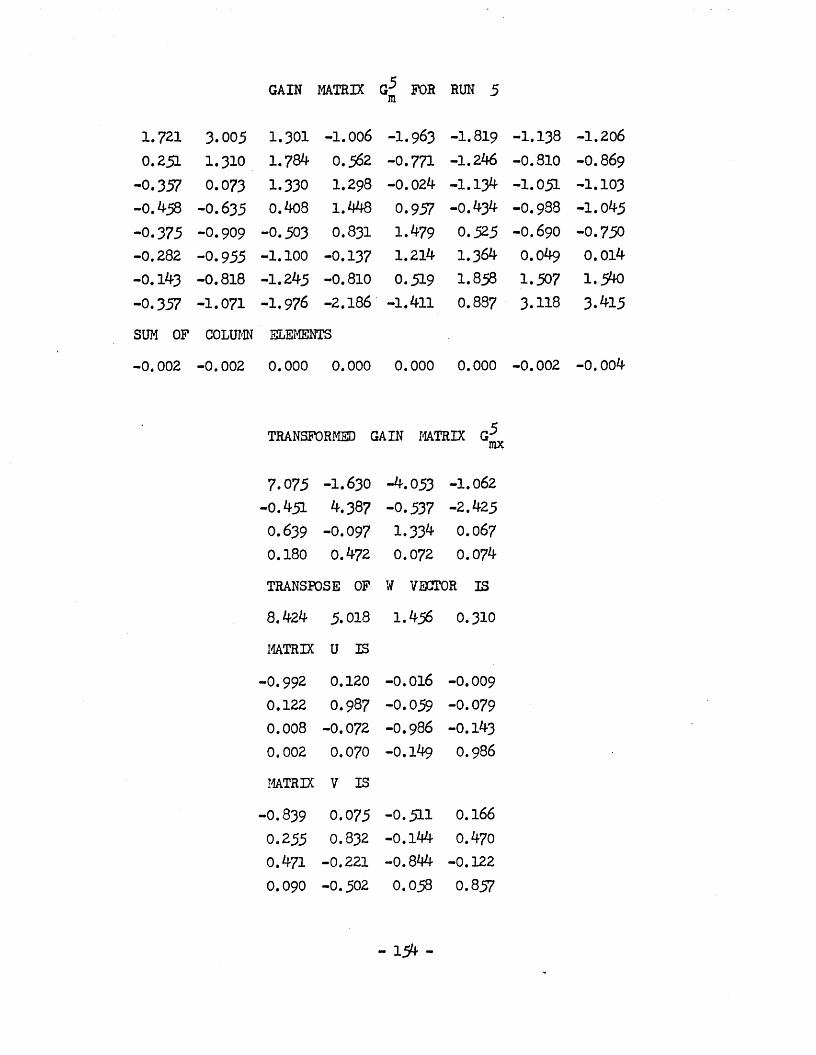
GAIN MATRIX G*5 FOR RUN 5m

1.721 3.005 1.301 -1.006 -1.963 -1.819 -1.138 -1.206

0.251 1.310 1.784 0.562 -0.771 -1.246 -0.810 -O.869

-0.357 0.073 1.330 1.298 -0.024 -1.134 -1.051 -1.103-0.458 -0.635 0.408 1.448 0.957 -0.434 -O.988 -1.045-0.375 -0.909 -0.503 0.831 1.479 0.525 -O.69O -0.750-0.282 -0.955 -1.100 -0.137 1.214 1.364 0.049 0.014-0.143 -0.818 -1.245 -0.810 0.519 1.858 1.507 1.540-0.357 -1.071 -1.976 -2.186 -1.411 0.887 3.118 3.415SUM OF COLUMN ELEMENTS

-0.002 -0.002 0.000 0.000 0.000 0.000 -0.002 -0.004

TRANSFORMED GAIN MATRIX Gmx

7.075 -1.630 -4.053 -1.062-0.451 4.387 -0.537 -2.425

0.639 -0.097 1.334 0.0670.180 0.472 0.072 0.074TRANSPOSE OF W VECTOR IS8.424 5.018 1.456 0.310MATRIX U IS

-0.992 0.120 -0.016 -0.0090.122 0.987 -0.059 -0.0790.008 -0.072 -O.986 -0.1430.002 0.070 -0.149 0.986

MATRIX V IS-0.839 0.075 -0.511 0.166

0.255 0.832 -0.144 0.4700.471 -0.221 -0.844 -0.1220.090 -0.502 0.058 0.857

- 154 -

GAIN MATRIX G6 FORm RUN 6

1.420 2.846 1.839 -0.731 -1.974 -1.909 -1.092 -1.156

O.15B 1.140 1.742 0.637 -0.744 -1.251 -O.698 r0.762

-0.327 0.021 1.135 1.243 -0.037 -1.166 -1.000 -1.064-0.398 -0.599 0.261 1.321 0.847 -0.525 -0.944 -1.013-0.328 -0.864 -0.579 0.750 1.359 0.374 -0.651 -0.717-0.240 -0.907 -1.125 -0.114 1.200 1.203 0.017 -0.016

-0.091 -0.758 -1.280 -0.755 0.688 1.955 1.458 1.510-0.244 -0.957 -1.99^ -2.249 -1.232 1.323 2.823 3.122

SUM OF COLUMN ELEMENTS

-0.051 -0.076 0.000 0.102 0.105 0.003 -0.089 -0.098

TRANSPORT® GAIN MATRIX G6nix

6.72 8 -1.640 -4.498 -I.069-0.425 3.857 -0.604 -2.3660.650 -0.199 0.968 0.0610.290 0.456 -0.005 -0.042TRANSPOSE OF W VECTOR IS8.348 4.585 1.138 0.254MATRIX U IS

-0.996 0.078 0.003 -0.0230.080 0.989 -O.O69 -0.101-0.006 -0.088 -0.976 -0.195-0.016 0.087 -0.203 0.975MATRIX V IS

-0.808 0.016 -0.561 0.1760.232 0.816 -0.150 0.506

0.530 -0.226 -0.808 -0.1180.104 -0.530 0.095 0.835

- 155 -

GAIN MATRIX G7 FOR RUN 7m

1.278 2.837 2.283 -0.531 -2.026 -2.018 -1.119 -1.162

0.119 1.04? 1.664 0.629 -0.755 -1.252 -0.591 -0.638

-0.302 -0.013 0.969 1.185 -0.019 -1.159 -0.913 -0.971-O.367 -0.593 O.129 1.204 0.761 -0.605 -0.893 -0.963-0.301 -0.828 -0.618 0.693 1.225 0.205 -0.599 -0.674

-0.195 -0.839 -1.107 -0.073 1.171 1.085 0.097 0.051-0.060 -0.703 -1.307 -0.741 0.775 2.060 1.540 1.592-0.168 -0.906 -2.013 -2.367 -1.132 1.684 2.479 2.766

SUM OF COLUMN ELEMENTS0.003 -0.000 -0.000 -0.000 -0.000 -0.001 0.001 0.000

TRANSFORMED GAIN MATRIX G?mx

6.538 -1.595 -4.862 -1.050-0.274 3.427 -0.617 -2.3380.667 -0.248 O.616 0.0450.481 0.404 -0.082 -0.126

TRANSPOSE OF W VECTOR IS

8.383 4.231 0.893 0.217

MATRIX U IS-0.998 -0.031 0.036 0.035

0.033 -0.991 -0.050 0.116

-0.025 0.084 -0.942 0.321-0.042 -0.095 -0.327 -0.938MATRIX V IS

-0.784 0.018 -0.598 -0.162

0.202 -0.805 -0.143 -0.5380.575 0.195 -0.783 0.1320.116 0.559 0.086 -0.816

- 156 -

GAIN MATRIX G8 FORm RUN 8

2.475 3.068 0.286 -1.269 -1.685 -1.461 -1.118 -1.1910.287 1.295 1.496 0.318 -0.797 -1.113 -0.886 -0.936-0.467 0.126 1.522 1.275 -0.041 -0.973 -O.998 -1.030

-0.577 -0.613 0.625 1.492 0.971 -0.317 -O.962 -0.994-0.480 -0.907 -0.379 0.817 1.518 0.710 -0.630 -0.671-0.400 -0.966 -0.966 -0.174 1.134 1.530 0.229 0.201-0.319 -0.899 -1.101 -0.831 0.197 1.515 1.531 1.548-0.519 -1.105 -1.484 -1.625 -1.299 0.108 2.832 3.075SUM OF COLUMN ELEMENTS-0.000 -0.001 -0.001 0.002 -0.002 -0.002 -0.003 0.001

TRANSFORMED GAIN MATRIX G8mx

6.85L -1.040 -2.7*K) -0.902 -0.078 4.605 -0.249 -2.0660.415 0.350 1.886 0.1070.307 0.290 0.185 0.331TRANS BOSE OF W VECTOR IS7.534 5.033 1.951 0.4l4MATRIX U IS

-0.99^ 0.091 -0.046 -0.027O.O89 0.995 0.039 -0.0190.053 0.030 -0.981 -0.179-0.016 0.027 -0.180 0.983

MATRIX V IS-0.902 0.112 -0.402 0.1010.194 0.895 -0.086 0.3910.371 -0.086 -0.905 -0.1850.094 -0.422 -0.104 0.895

- 157 -

GAIN MATRIX G9 FOR RUN 9in

1.698 2.032 0.449 -0.695 -1.139 -1.083 -0.814 -0.8580.228 0.750 0.958 0.288 -0.427 -0.701 -0.560 -0.604

-0.344 -0.023 0.910 0.860 0.095 -0.572 -0.687 -0.735-0.409 -0.417 O.36I 0.944 0.710 -0.032 -0.6l6 -0.671

-0.337 -0.564 -0.272 0.466 O.962 0.567 -0.323 -0.379-0.282 -0.591 -0.663 -0.185 0.640 0.998 0.267 0.249-0.202 -0.517 -0.726 -0.561 0.078 0.951 1.128 1.193-0.350 -o. 665 -1.014 -1.116 -0.919 -0.079 1.603 1.805

SUM OF COLUMN ELEMENTS-0.000 -0.000 0.002 0.000 0.000 -0.002 -0.002 0.000

TRANSFORMED GAIN MATRIX G9mx

4.512 -0.900 -1.742 -0.4080.226 2.990 -0.357 -1.2880.224 0.363 1.069 -0.0170.346 0.122 0.098 0.144TRANSPOSE OF W VECTOR IS

4.951 3.290 1.126 0.195MATRIX U IS

-0.996 0.042 -0.035 -0.059.0.039 0.995 0.082 -0.0070.051 0.077 -0.971 -0.219

-0.049 0.027 -0.220 0.973MATRIX V IS

-0.907 0.135 -0.387 0.0870.207 0.902 -O.O89 0.3650.357 -0.104 -0.912 -0.1680.070 -0.39^ -0.094 0.911

- 158 -

GAIN MATRIX G FOR RUN 10m

2.615 3.789 0.687 -1.334 -1.654 -1.339 -1.041 -1.1100.470 2.034 2.231 0.258 -1.349 -1.819 -1.407 -1.426-0.439 0.294 1.962 1.499 -0.378 -1.656 -1.532 -1.538-0.711 -0.932 0.623 1.937 1.135 -0.746 -1.468 -1.484-0.617 -1.372 -0.739 1.050 1.969 0.669 -1.007 -1.052-0.503 -1.437 -1.568 -0.413 1.405 1.908 0.258 0.215-0.447 -1.334 -1.745 -1.374 0.050 2.043 2.075 2.092

-0.362 -1.035 -1.447 -1.613 -1.174 0.995 4.126 4.308SUM OF COLUMN ELEMENTS0.004 0.006 0.004 0.010 o.oo4 0.004 0.002 0.004

TRANSFORMED GAIN MATRIX Gmx

8.953 -1.470 -4.142 -1.335-0.652 5.2 43 -0.367 -2.686-0.132 0.381 2.654 0.2230.087 -0.191 0.350 0.766

TRANSPOSE OF W VECTOR IS10.202 5.882 2.360 0.537MATRIX U IS

-0.983 0.115 -0.138 0.0020.121 0.987 -0.037 0.0940.133 -0.040 -0.979 -0.1450.010 -0.100 -0.140 0.984MATRIX V IS

-0.872 0.065 -0.466 O.1290.208 0.852 -0.144 0.4570.430 -0.166 -0.872 -0.1610.100 -0.491 -0.016 0.864

- 159 -

GAIN MATRIX G FOR RUN 11m

2.496 3.443 0.612 -1.201 -1.675 -1.451 -1.093 -1.178

0.475 1.693 1.767 0.270 -1.065 -1.460 -1.199 -1.270

-0.459 0.161 1.695 1.413 -0.124 -1.223 -1.282 -1.347-0.660 -0.785 0.641 1.717 1.101 -0.425 -1.230 -1.299

-0.554 -1.123 -0.518 0.922 1.744 0.781 -0.334 -0.903-0.446 -1.174 -1.217 -0.285 1.256 1.741 0.216 0.188-0.390 -1.119 -1.443 -1.146 0.053 1.655 1.789 1.867-0.458 -1.095 -1.537 -1.688 -1.289 0.384 3.639 3.943SUM OF COLUMN ELEMENTS

-0.001 -0.001 -0.001 0.002 0.001 0.001 -0.001 -0.001

TRANSFORMED GAIN MATRIX Gmx

8.056 -1.525 -3.323 -1.113-0.424 5.090 -0.478 -2.35L0.225 0.281 2.144 0.1140.123 -0.016 0.209 0.522

TRANSPOSE OF W VECTOR IS

8.997 5.563 2.081 0.449MATRIX U IS

-0.987 0.138 -0.079 -0.0010.140 O.988 -0.025 0.0450.076 -0.030 -0.989 -0.1180.001 -0.049 -0.117 0.991MATRIX V IS

-0.888 0.122 -0.418 0.1420.249 0.865 -0.135 0.4120.375 -0.181 -0.397 -0.1410.086 -0.450 -0.012 0.888

- 160 -

GAIN MATRIX G FOR RUN 12m

2.325 3.065 0.353 -1.214 -1.602 -1.368 -1.073 -1.1480.366 1.381 1.522 0.347 -0.793 -1.137 -0.937 -0.983-0.436 0.130 1.492 1.247 -0.076 -1.038 -1.099 -1.132-0.572 -0.634 0.619 1.481 0.962 -0.335 -1.035 -1.072-0.477 -0.933 -0.376 0.820 1.507 0.695 -0.695 -0.7^4-0.395 -0.995 -0.991 -0.188 1.109 1.479 0.140 0.108-0.292 -0.894 -1.103 -0.820 0.223 1.517 1.516 1.532-0.518 -1.120 -1.512 -1.677 -I.330 0.181 3.181 3.440SUM OF COLUMN ELEMENTS-0.000 -0.001 0.002 -0.003 0.001 -0.005 -0.002 0.000

TRANSFORMED GAIN MATRIX G12mx

7.025 -1.248 -2.787 -0.915 -0.352 4.635 -0.295 -2.091

0.455 0.190 1.873 0.1110.138 0.290 0.171 0.305TRANSPOSE OF W VECTOR IS

7.778 5.020 1.930 0.385MATRIX U IS

-O.986 0.157 -0.043 -0.0050.158 0.987 -0.010 -0.0240.040 -0.019 -0.989 -0.1330.004 0.022 -0.134 O.99OMATRIX V IS

-O.895 0.150 -O.39S 0.1270.253 0.872 -0.113 0.4010.357 -0.152 -0.908 -0.1520.074 -0.438 -0.047 0.894

- 161 -

GAIN MATRIX G13 FORm RUN 13

2.438 3.286 0.415 -1.247 -1.634 -1.413 -1.104 -1.1800.392 1.553 1.688 O.296 -0.950 -1.286 -1.057 -1.110

-0.470 0.117 1.632 1.351 -0.140 -1.133 -1.164 -1.206

-0.612 -0.733 0.621 1.643 1.037 -0.4o6 -1.117 -1.164-0.506 -1.030 -0.473 0.876 1.676 0.731 -0.776 -0.834-0.421 -1.081 -1.112 -0.265 1.208 1.657 0.167 0.130

-0.336 -1.002 -1.261 -1.001 0.110 1.624 1.662 1.697-0.488 -1.110 -1.510 -1.653 -1.305 0.224 3.388 3.668SUM OF COLUMN ELEMENTS

-0.005 -0.001 0.001 0.000 0.000 -0.003 -0.002 -0.001

TRANSFORMED GAIN MATRIX G13mx

7.517 -1.351 -3.056 -1.031 0.353 4.887 -0.389 -2.2500.357 0.250 2.093 0.1030.153 0.140 0.208 0.471TRANSPOSE OF W VECTOR IS8.356 5.331 2.093 0.472MATRIX U IS

-O.988 0.138 -0.065 -0.0040.139 0.989 -0.015 0.0160.063 -0.022 -O.988 -0.1350.001 -0.019 -0.134 0.990MATRIX V IS

-0.892 0.128 -0.411 0.1350.243 0.870 -0.122 0.4090.370 -0.161 -0.902 -0.1460.085 -0.446 -0.029 0.890

- 162 -

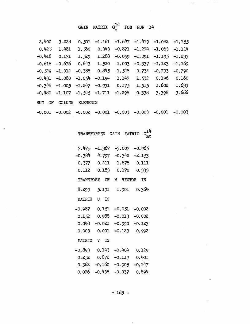
GAIN MATRIX 14 G FORm RUN 14

2.400 3.228 0.501 -1.161 -1.647 -1.419 -1.082 -1.1550.42 5 1.481 1.560 0.343 -O.871 -1.274 -1.063 -1.114

-0.418 0.171 1.529 1.288 -0.059 -1.091 -1.195 -1.233-0.618 -O.676 0.643 1.520 1.003 -0.337 -1.123 -1.169

-0.529 -1.012 -O.388 0.845 1.5*18 0.732 -0.733 -0.790-0.431 -1.080 -1.054 -0.194 1.147 1.532 0.196 0.160-0.348 -1.005 -1.247 -0.931 0.175 1.515 1.602 1.633-0.480 -1.107 -1.545 -1.711 -1.298 0.338 3.398 3.666

SUM OF COLUMN ELEMENTS-0.001 -0.002 -0.002 -0.001 -0.003 -0.003 -0.001 -0.003

TRANSFORMED GAIN MATRIX G Zmx

7A75 -1.367 -3.007 -0.965 -0.384 4.797 -0.342 -2.1530.377 0.211 1.878 0.1110.112 0.183 0.170 0.333TRANSPOSE OF W VECTOR IS

8.299 5.191 1.901 0.364MATRIX U IS

-0.937 0.151 -0.051 -0.0020.152 O.988 -0.013 -0.0020.048 -0.021 -0.990 -0.123

0.003 0.001 -0.123 0.992MATRIX V IS

-0.893 0.143 -0.404 0.1290.252 0.8 72 -0.119 0.4010.362 -0.160 -0.905 -0.1470.076 -0.438 -0.037 O.894

- 163 -

GAIN MATRIX G1-5 FOR RUN 15m

2.452 3-354 0.297 -1.379 -1.601 -1.3^3 -1.100 -1.1730.215 1.559 1.894 0.282 -1.068 -1.309 -1.000 -1.049

-0.542 0.081 1.836 1.487 -0.265 -1.276 -1.137 -1.175-0.565 -0.793 0.605 1.822 1.079 -0.570 -1.166 -1.206

-0.419 -1.056 -0.637 0.915 1.862 0.722 -0.889 -0.944-0.349 -1.062 -1.234 -0.364 1.343 1.635 0.082 0.044-0.292 -0.962 -1.268 -1.078 0.114 1.804 1.679 1.711-0.497 -1.120 -1.490 -1.683 -1.462 0.136 3.532 3.797SUM OF COLUMN ELEMENTS0.002 0.000 0.003 0.002 0.003 -0.001 0.002 0.003

TRANSFORMED GAIN MATRIX G1-5mx

7.526 -1.434 -3.232 -1.084-0.496 5.056 -0.444 -2.4770.402 0.228 2.487 0.1600.212 0.197 0.301 0.624TRANSPOSE OF W VECTOR IS8.482 5.573 2.460 0.622MATRIX U IS

-0.982 0.163 -0.090 -0.0060.168 0.984 -0.049 0.0200.081 -0.059 -O.98I -O.I630.003 -0.029 -0.162 O.986

MATRIX V IS

-0.877 0.127 -0.440 0.1390.268 0.847 -0.152 0.4310.339 -0.201 -0.834 -0.1590.078 -0.474 -0.015 0.876

- 1 6 4 -

GAIN MATRIX

2.333 3.096 0.583 -1.032

0.570 1.499 1.408 0.301-0.310 0.225 1.357 1.149-0.609 -0.614 0.6l4 1.388

-0.537 -0.975 -0.283 0.819-0.506 -1.085 -0.933 -0.128-0.403 -1.035 -1.205 -0.861

-0.485 -1.108 -1.540 -I.638

SUM OF COLUMN 2LEH3NTS0.002 0.003 -0.004 -0.001

r° FOR RUN 16m

-1.603 -1.474 -1.116 -1.195-0.775 -1.211 -1.107 -1.1750.014 -0.943 -1.199 -1.2590.962 -0.204 -1.058 -1.1211.408 0.726 -0.627 -0.6881.018 1.384 0.276 0.2530.140 1.367 1.603 1.662

-1.165 0.355 3.232 3.525

0.001 0.000 0.003 0.000

TRANSFORM GAIN MATRIX Gl6mx

7.444 -1.323 -2.771 -0.926-0.266 4.568 -0.332 -1.9400.286 0.200 1.533 0.0790.077 0.109 0.113 0.269TRANSPOSE OF W VECTOR IS

8.153 4.913 1.552 0.281MATRIX U IS

-0.991 0.126 -0.038 -0.0010.126 0.991 -0.001 0.0030.038 -0.006 -0.994 -0.1000.001 -0.004 -0.100 0.994MATRIX V IS

-0.907 0.131 -0.374 0.1280.232 0.887 -0.107 0.3310.338 -•0.l40 -0.919 -0.1390.082 -•0.415 -0.042 0.904

- 165 -

GAIN MATRIX 1G17 FORm RUN 17

2.664 3.589 0.542 -1.298 -1.781 -1.545 -1.198 -1.2760.441 1.658 1.779 0.325 -1.019 -1.425 -1.184 -1.246-0.467 0.154 1.740 1.453 -O.O98 -1.214 -1.290 -1.342-0.675 -0.779 O.69O 1.748 1.128 -0.401 -1.229 -1.286-0.565 -1.121 -0.484 0.954 1.772 0.812 -0.830 -O.896-0.464 -1.180 -1.197 -0.250 1.294 1.761 0.200 0.161

-0.389 -1.111 -1.399 -1.084 0.138 1.708 1.777 1.821-0.523 -1.204 -1.668 -1.846 -1.437 0.303 3.755 4 .068

SUM OF COLUMN ELEMENTS0.000 0.004 0.003 0.002 -0.003 0.001 0.000 0.003

TRANSFORMED GAIN MATRIX G17mx

8.255 -1.533 -3.328 -1.091

-0.405 5.329 -0.430 -2.4200.409 0.240 2.182 0.1220.138 0.159 0.204 0.462TRANSPOSE OF W VECTOR IS9.172 5.789 2.195 0.469MATRIX U IS

-0.987 0.146 -0.058 -0.0020.148 O.988 -0.020 0.0100.054 -0.027 -0.990 -0.1250.003 -0.014 -0.125 0.992MATRIX V IS

-0.892 0.138 -0.407 0.1330.252 0.869 -0.126 0.4o40.364 -0.162 -0.904 -0.1460.071 -0.442 -0.030 0.892

- 166 -

GAIN MATRIX G FOR RUN 18m

2 .486 3.325 0.429 -1.246 -1.700 -1.468 -1.139 -1.216

0.424 1.547 1.675 0.348 -0.916 -1.292 -1.071 -1.125-0.462 0.144 1.635 1.365 -0.086 -1.125 -1.194 -1.237-0.629 -0.714 0.660 1.622 1.056 -0.366 -1.137 -1.184-0.523 -1.033 -0.435 0.882 1.657 0.766 -0.769 -0.825-0.429 -1.092 -1.100 -0.229 1.216 1.648 0.180 0.147-0.342 -1.011 -1.264 -0.973 0.167 1.619 1.663 1.698

-0.526 -1.165 -1.597 -1.768 -1.391 0.215 3.466 3.744SUM OF COLUMN ELEMENTS-0.002 0.001 0.002 0.001 0.002 -0.002 -0.002 0.001

TRANSFORMED GAIN MATRIX G "mx

7.669 -1.409 -3.076 -0.996 -0.370 5.006 -0.376 -2.2670.401 0.225 2.051 0.1190.134 0.208 0.193 0.391

TRANSPOSE OF W VECTOR IS8.512 5.430 2.073 0.425

MATRIX U IS-O.986 0.151 -0.056 -0.0030.152 O.988 -0.016 -0.002

0.053 -0.024 -O.989 -0.129

0.003 -0.001 -0.129 0.991

MATRIX V IS

-0.893 0.144 -0.405 0.1300.254 0.870 -0.121 0.4030.362 -0.163 -0.905 -0.1480.075 -0.440 -0.036 0.893

- 167 -

GAIN MATRIX G19 TORIQ RUN 19

2.309 3.153 0.448 -1.167 -1.564 -1.346 -1.032 -1.106

0.392 1.468 1.590 0.296 -0.910 -1.260 -1.036 -1.087-0.420 0.138 1.545 1.278 -0.121 -1.101 -1.154 -1.195-0.592 -0.695 0.609 1.543 0.985 -0.370 -1.099 -1.145-0.497 -1.000 -0.436 0.841 1.573 0.712 -0.746 -0.802-0.408 -1.055 -1.075 -0.234 1.146 1.551 0.170 0.136-0.332 -0.979 -1.239 -0.959 0.126 1.519 1.581 1.614-0.449 -1.032 -1.442 -1.596 -1.232 O.297 3.318 3.586SUM OP COLUMN ELEMENTS0.000 0.003 0.000 0.002 0.003 0.002 0.001 -0.001

TRANSFORMED GAIN MATRIX G19mx

7.254 -1.321 -2.956 -0.988-0.388 4.675 -0.377 -2.1480.318 0.223 1.956 0.1020.118 0.120 0.185 0.410TRANSPOSE OF W VECTOR IS8.074 5.092 1.946 0.407MATRIX U IS

-0.937 0.146 -0.065 -0.002

0.147 O.988 -0.020 0.0150.062 -0.027 -O.989 -0.123

0.003 -0.018 -0.123 0.992MATRIX V IS

-O.89I 0.130 -0.411 0.1380.248 0.863 -0.125 0.4100.369 -O.I69 -O.902 -0.l4l0.082 -0.44 7 -0.022 0.890

- 1 6 8 -

GAIN MATRIX G FOR RUN 20m

2.440 3.202 0.488 -0.981 -1.254 -0.950 -0.605 -0.6530.232 1.374 l >75 0.108 -1.181 -1.564 -1.275 -I.298

-0.448 0.136 1.540 1.234 -0.212 -1.215 -1.204 -1.217

-0.658 -0.771 0.553 1.484 0.905 -0.494 -1.163 -1.204-0.563 -1.087 -0.506 0.769 1.503 0.6o4 -0.747 -0.827-0.445 -1.108 -1.120 -0.291 I.O96 1.488 0.299 0.248-0.551 -1.227 -1.506 -1.268 -0.192 1.233 1.470 1.545-0.024 -0.5L9 -0.917 -1.053 -0.663 0.899 3.229 3.412SUM OF COLUMN elements

0.002 -0.001 0.007 0.004 0.001 -0.000 0.002 0.005

TRANSFORMED GAIN MATRIX G2°mx

7.435 -1.245 -3.060 -1.052-0.176 4.736 -0.422 -2.1600.270 0.369 1.954 0.0320.320 0.047 0.168 0.425TRANSPOSE OF W VECTOR IS8.245 5.193 1.949 0.4l6MATRIX U IS

-0.993 0.092 -0.065 -0.029

0.090 0.995 0.013 0.0310.071 0.011 -0.984 -0.159

-0.020 -0.025 -0.161 0.986

MATRIX V IS-0.895 0.097 -0.415 0.1240.205 0.885 -0.115 0.4000.380 -0.131 -0.900 -0.1640.102 -0.434 -0.056 0.893

- 169 -

GAIN MATRIX 21G FORm RUN 21

2.5^9 3.319 0.491 -1.172 -1.509 -1.333 -1.051 -1.095

0.373 1.550 1.699 0.228 -1.006 -1.3^2 -1.087 -1.106

-0.463 0.167 1.601 1.277 -0.199 -1.178 -1.168 -1.180-0.628 -0.724 0.590 1.610 0.971 -0.471 -1.119 -1.133-0.530 -1.057 -0.499 0.894 1.632 0.642 -0.778 -0.799-0.440 -1.114 -1.146 -0.239 1.213 1.578 0.143 0.128-0.374 -1.049 -1.315 -1.019 0.120 1.601 1.5^7 1.551-0.463 -1.088 -1.422 -1.577 -I.223 0.503 3.513 3.637SUM OF COLUMN ELEMENTS0.000 0.002 0.000 0.001 0.000 0.001 0.000 0.001

TRANSFORMED GAIN MATRIX G21mx

7.521 -1.190 -3.175 -O.98I-0.359 4.695 -0.250 -2.219

0.379 0.226 2.068 0.2170.093 0.104 0.228 0.508TRANSPOSE OF W VECTOR IS8.364 5.152 2.079 0.463MATRIX U IS

-0.990 0.121 -0.067 0.0020.122 0.991 -0.023 0.0260.063 -0.027 -0.987 -0.1440.008 -0.031 -0.143 0.989

MATRIX V IS-0.892 0.104 -0.426 0.1010.211 0.874 -0.129 0.4170.388 -0.135 -O.89I -0.189

0.085 -0.45^ -0.081 0.882

- 170 -

GAIN MATRIX G FOR RUN 22m

-0.015 -0.021 -0.028 -0.034 -0.040 -0.046 -0.052 -0.0570.015 0.019 0.023 0.028 0.033 0.037 0.04l 0.044

-0.001 -0.001 -0.000 0.000 0.001 0.002 0.002 0.0030.002 0.003 0.004 0.005 0.007 0.008 0.009 0.0100.002 0.003 0.004 0.005 0.007 0.008 0.009 0.010-0.001 -0.001 -0.000 0.000 0.001 0.002 0.002 0.003

0.015 0.019 0.023 0.028 0.033 0.037 0.04l 0.044-0.015 -0.021 -0.028 -0.034 -o. o4o -o.o46 -O.052 -0.057

- 171 -

Rack 1 Rack 8

o©-

fiO 26.^^X d i s t a n c e

oo 42.^^ 7^ . ^

eo

CO

R H 0 6Mf1 CHG W = 1 . 4f1

Fig. 6.1a.

Rack 2CD

CO

7^.^^42.20 .^^ STANCE

14 .00^^

a :

CJCO

CO

RZ*7 6Mn CHG Wni .4(1r»>

- 172 -

SHP

CHAN

GF

*10

SHP

CH

AN

GE

oRack 3

o-co

oOQ ^^ 14 .0 0 fB . 42.00 56/^^ no .^^

R346 6 nn CHG W r l .4

oRack 4oao-

o-

56 .00 70 .00.00,8 .00.00

o _

to

o _

R4<5 6fin CHG W =Pig. 6.Id.

Fig. 6.1. Shape profiles for RUN 0.

- 173 -

ooRack 1 — Rack 8 -*■

t—i lC’— 1—' cn

acd

o .00 GO 70 -GO

•STANCEao-1— o LJ o

GO o _oR U 8 6MM CHG Wzl ,7M

Rackoo Rack/— )tc>— i—> cn

oo

7 0 - 0 056 -002 6 - 0 0I ST A NCE

M .0000

a:a(_J o

GO CD.

CDID R2&7 611(1 C H G W=1 .711

Pig. 6.2b.I

- 1 7k -

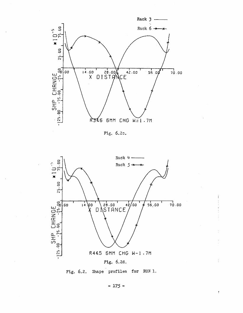
Rack 3o

J - i o

oo

00 S. 00, 55 0 70 -00

CL

CO o _o

6 6MM CHG W=1.7M

Fig. 6.2c.

Racko Rack

4 2 / 0 0 55 -002 9 . 0 0STANCE

70 -0000

CL

CO

_r>CJ R445 6 MM CHG W-l ,7M Fig. 6.2d.

Fig. 6.2. Shape profiles for RUN 1.

- 175 -4

ooin Rack 1Rack 9-*

oCD

8^ .^^ 100 . 0 00 00 60 040 -00X D I S T f l N

130

cco _

oCDQ_

GO c?_oo R H 8 6MM CHG U~ 1 .6M

Fig. 6,33..

oRack 2

oo

o70 00/ 20-00 *

D I S T A N C E4Z • 56 0014 00

CEo _oa<n

CL

GO o _CD

CD R247 6MM CHG W=1.6MFig. 6.3b.

- 176 -

ooRackRack

oo-40

00 14 .00 29 .0, 7 0 - 0 0

cc o _CD

CDan

CD o _o

R346 6MM CHG W=1-6M

Fig. 6.3c.

CD

Rack 4

CDCD

CD— 4C

CD

°0 70 .00.009 . 0 000ANG

cc o _oLJ oCDCL

CO o _oR465 6Mf1 CHG W=1 .6M

Fig. 6.3d.

Fig. 6.3. Shape profiles for RUN 2,

- 177 -

ooRack 1

u>

42 .00 56 .00 70 .00to 2 8 - 0 0X D I S T A N C E

14

CL o _

o

CO

iFig. 6.4a.

oU1 RackRack

o-CO

56 .00 70 .0014 .00 42 .^^

coa_co o _

R2*7 6nn CHG VJ=1 .5M Fig. 6.4b.

- 178 -

Rack 3 Rack 6

oa-m

16 -00 48 . ^ 64 . ^^^ 3^ . ^

CL~r~ ° -

R 3 4 6 6 n n C H G W=1 .511

Fig. 6. c.

CM-*

ORack ----Rack 5 -*— *

o

1 6\^^ 32.^^ / *

S T A N C E80 .^^4^/^^ 64 .00^^

XCO

CD R4£>5 6MM CHG U = 1 .5f1Fig. 6.4d

Fig. 6 A, Shape profiles for RUN 3*

- 179 -

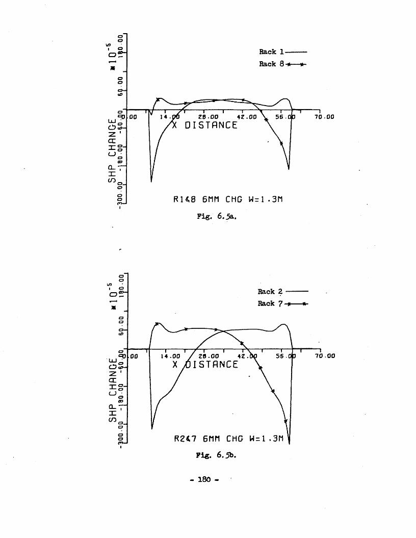
Rack 1

iO

70-0000 28-00 - D I S T A N C E

4 2 . 0 0

CC3Z

CDQ_CO

R U 8 6MM CHG U - 1 .3HiFig. 6.5a.

aoo Rack

RackO

(O

70 0055 ■ 0 314 .00 4200occ

CDCLXco

R247 6nf1 CHG W=1 .3HiFig. 6 .5b.

- 1 8 0 -

ooi o□ r Rack

Rack

2 9 . 70 -0000 42 .00 • 00

cr

on

CD C5_oR346 6MM CHG W=1.3M

Fig. 6.5c.

OORackRack

o

00 2 .00 70 00

c e o _CJ o

ana_oo o _

o

Fig. 6.5* Shape profiles for RUN 4.

- 181 -

ooRack 1

o i H

si

70 00005542 .002 5 - 0 0D I S T A N C E

00

a:oCPQ_

COsi

R 148 6nn CHG W=1 -2(1§ Jpo—Ii

Fig. 6.6a.

o

Rack 2o

oo

70 -0000562 5 . 0 0 <STANCE

1 4 .00<=0 u j ■c7> 5-CEnr °--1— QLJ • o

CD0-7“co 0-1

R2£7 6MM CHG W=1 .2MFig. 6.6b.

- 182 -

oRack 3 — Rack 6-*

I o ^ C O -

70.DO14 .0000 42 .00TNC

cc o _oCD

Ic.CO o _o

o R3£6 6MM CHG Wri,2M

ooRack k Rack 5

oo

70 0055 .00.00 2 .0000

CC o _ooCD

CO o _

o R4«,5 6MM CHG W=1 .2M Fig. 6.6d.

Fig. 6.6. Shape profiles for RUN 5.

- 183 -

oa Hack 1— Hack 8-*

CDCD

oH

7 0 -00e -ooZS -00D I S T A N C E

.00loo

cc

CJ C3

COsi

I

ooRack 2

oo

7 0 - 0 056 -004 Z \ 0 0Z9 -00STANCE

00oLlJ

cc §1CMCL.

COsiR2&7 W=1. 1M 6P1M C

- -

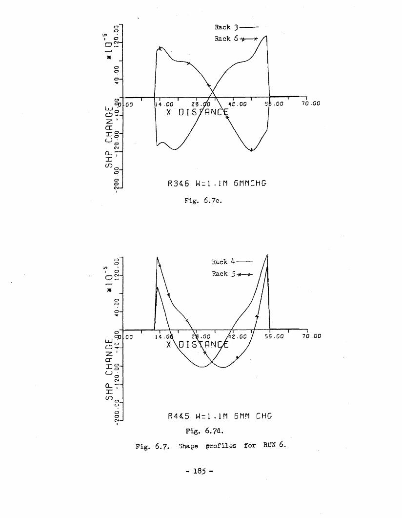
Rack 3CDCD

CDCD

O-

CD5 .0042 .004 .0000UJ

CD

CCT" CDCJ •C3<NQ-7“zc

oCD CD CJ—1 l

R3^6 . i n 6nnchG

Fig. 6.7c.

Rack ^---Rack 5-*— *■

oo

oo-

7 0 - 0 05 5 -042 -000StflN

ccT °- -L- OCJ •

CDCJ

Q-7"JZ^ o _

CD

R4«.5 w = i . m gnn chg-

Fig. 6.7<1.Fig. 6.7. Shape profiles for RUN 6.

- 185 -

ooI oo ^ “ Rack 1

Rack 8ooo—

0 -CO55 002 3 - 0 0

X/ DISTANCEtoooo

c d

ccT ° - o

Q_CO o _c?

ooC>i—1I

R H 8 W=1M 6rin CHGFig. 6.8a

oouOI o Rack 2□ r Rack 7ooo-'

O<=0

i.00 1 1 / 1 1 \ 1 00 /23.C0 4a.00 t i i55.00 70CD -r- X O/ i STf l NCE \:z ’ccx °--1— oLJ oCNQ_7"X00 o.o

oo (R247 W=1M 6MM CHOOJ-11

1 Fig. 6.3b.

- 186 -

Hack 3 Rack 6

o o

oc:

ooo-

70 .0042 -000000

CC-T- o _o

CL.

o _oooCM-1I

Fig. 6.8c.

o oo

o £!'Rack 4 Rack 5

ooo-

70 0014 .0000CDCTT- °- LJ o

CMQ_7“oo o _

R445 Wrin 6MP1 CHGFig. 6.8d.

Fig. 6.9. Shape profiles for RUN 7.

- 187 -

ooRack 1Rack 3

oo

7 0 -042 .0000D I S T A N C E

a:T" C3- oC_JoCD

0 - 7 “

CO

po-JIYS 50'/. MO R E

Fig. 6.9*.

OORack 2 Rack 7

oo

70 .0000 / 2 3 . 0 0X / D I STANCE

oo

ccoCOQ_

CO

o

Pig. 6.9^.

- 188 -

oC3Rack 3 Rack 6

ooo-<r

o70 .0042 .0014 .0000

ccc?_oCP

CLCO o _o

o YS 5 O X MOR E R3 4 6 1 .4I

o

Rack 4- Rack 5oo

cn-

oo

,8 .00 55 .00.0000A N

CCo

CO o _oo

Fig. 6.9d.Fig. 6.9. Shape profiles for RUN 3.

- I89 -

om o

Rack 1 Rack 2

o-n

70 .0042 .00 56 .0000

CO

U o

CO o _

RACKU7 W=1 .4Fig. 6.10a

Rack 2mRack 7

o -

14 .00 7 0 . 0 000 56 .00

CCo C_J o

RACK 247 W=1.4Fig. 6.10b

190 -

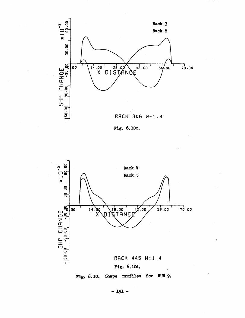
Rack 3 Rack 6

in

oo—o

00 14 .00 28 -0 42 .00 70 .00

cr(—) CD

Q_CJ-CO o_

RACK 3*6 W-l .4ini

Pig. 6.10c.

o Rack Rack 5

in

o-

56 .00 70 .0028 .00 'ST ANC

00

ccCJ CDQ_ 7-CO

oin RACK 4£5 W=1.4f

Fig. 6.10d.Fig. 6.10. Shape profiles for RUN 9.

- 191 -

Rack 1 Rack 8

oo->/>

70 .0 05 6 .0 000 42 .0 0

d~ r ° -

oW9

RACK 148 Ucl .4 Fi*. 6.11a.

Rack 2 Rack 7O

00 7 0 .0 056 .0 01 4 .0 0 20.00 <

I STANCELU o

CC

RRCK 247 W=1 .4VI

Fi«. 6.111)

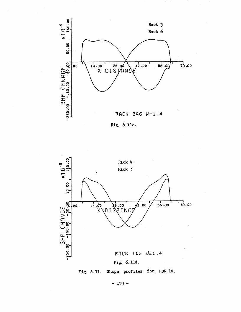
oo Rack 3

Rack 6I o

oIP

7 0 .0 056 .0i26 .0/ 42 .0 01 4 .0 000

o _

RACK 3*6 W=1 .4Fig. 6.11c.

o Rack 4 Rack 3

ooo -LO

7 0 .0 05 6 .0 0.00,8 .00TNC

X - °- -1— o(_J • o

1/3

0.7"XCO o _

o

RACK 4*5 U=1.4 Fig. 6.lid.

Fig. 6 .1 1 . Shape profiles for RUN 10.

- 193 -

oo

Rack 1 Rack 8

oO

o-

4 2 .0 026.^^DISTANCE

7 0 .0 05 6 .0 000i. 1 * oo S -a:nr

RACK 3 48incm-jFig. 6.12a

Rack Z Rack 7

i i14 .00

i r28 .00 5 6 .0 0

x d i s t a n c e

RACK Z*i7 Fig. 6.12b.

7 0 .0 0

- 19^ -

o Rack 3

Rack 6

o -vO

28 .a 42 .0014 .^^ 70.0056 100^^

CLo _

CLo _

IFig. 6.12c,

Rack Rack 5

oin

Oea­rn

7 0 -0 056 .008.00 X \D I 3\T A N C

.0014 .000

CL00 o _

RACK 4*5Fig. 6.12d.

Fig. 6.12. Shape profiles for RUN 11.

- 195 -

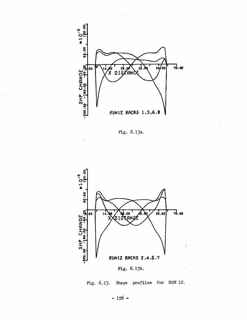
ooM •I O0 2 “

70.00

RUN12 RACKS 1.3,6,8

Fig. 6.13a.

a

56.00.00

9-J

RUN12 RACKS 2,4.5.7Fig. 6.13b.

Fig. 6.13. Shape profiles for RUN 12,

- 196 -

10.0056/00X Q1SJAN

RUN13 RACKS 1,3,6.8

Fig. 6.1^a.

56.00 70.00U.

RUN13 RACKS 2,4.5.7

Fig. 6.1 . Shape profiles for RUN 13.

- 197 -

i y I---------1— JP-------114.>80 28 .00 \ 42.X OIS/flN

S6/00

RUN!4 RACKS t .3.6,8

Fig. 6.15a.

56.00

RUN14 RACKS 2 , 4.5.1

Fig. 6.15b.

Fig. 6.15. Shape profiles for

i 170.00

“170.00

RUN 14.

- 198 -

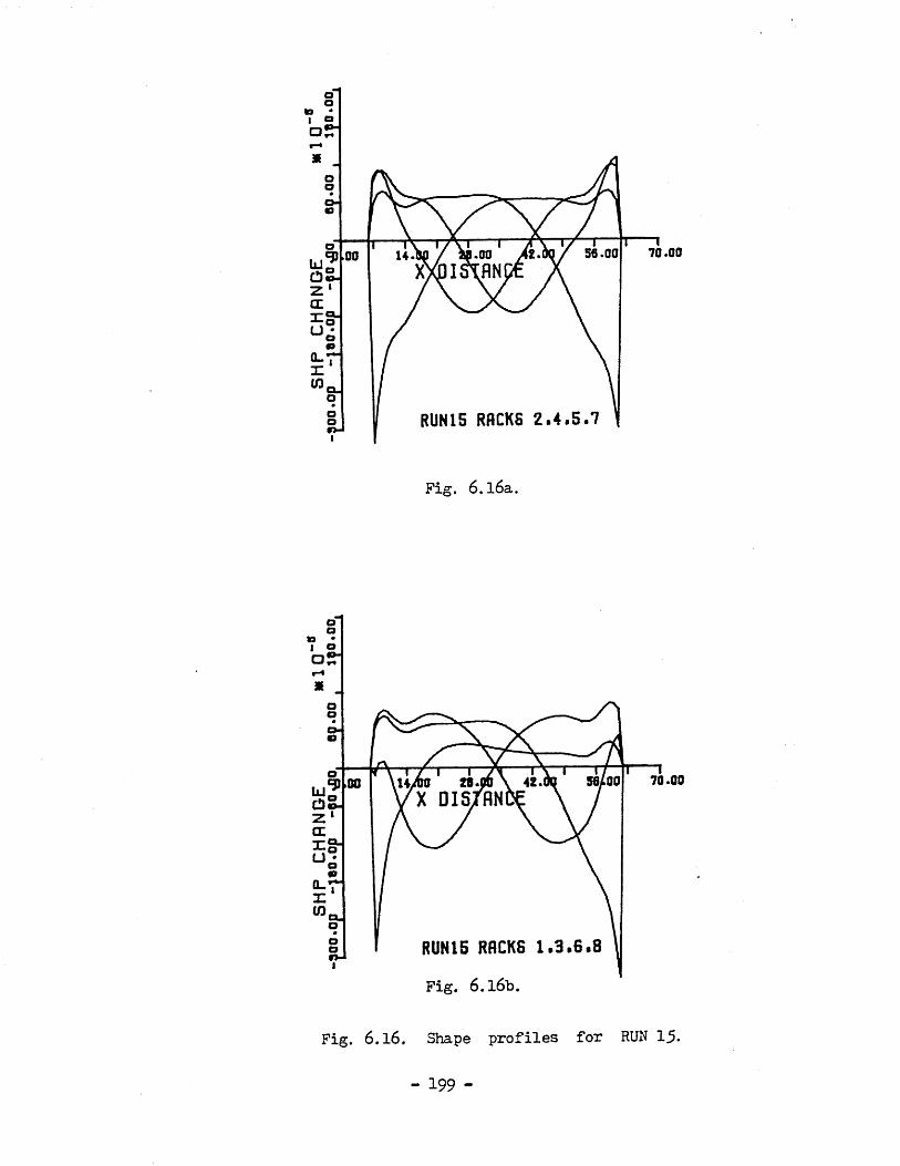
o

70.0056.00.00

RUN15 RACKS 2.4.5.7

Fig. 6.l6a.

70.0056/00!X DISJflN

RUN15 RACKS 1.3.6.8

Fig. 6.l6b.

Fig. 6.16. Shape profiles for RUN 15•

- 199 -

70.0056/00

RUN16 RflCKSl.3.6,8rvJ

Fig. 6.17a.

16.00 56.00

o RUN16 RACKS 2.4.5.7r>Ji

Fig. 6.17b.

Fig. 6.17. Shape profiles for RUN 16.

- 2 0 0 -

oo Rack 1 Rack 3

o

o-tn

70 -0 055 0042 . 0 000D I S T A N C E

R A C K U 8

Fig. 6.18a

oo Rack 2

Rack 7i o0 cn-

ooo -1/5

o <=0 LU •e>°-7 0 . 0 055 0 020.00

I S T A N C E14 . 0 000

a:-1— o

Q_XCO o _

Fig. 6.18b

- 201

Rack 3 Rack 6

oI o

oo-1/5

2 3 - 0 . 42 . 0 0 5 / 0 0 70 0000

CC

-1— o (_J o

i/5

0-7“cn o_o

RfiCK 3&6

Fig. 6.13c.

o Rack 4 Rack 5

ooo-U">o

U J^CZ)S-7 0 . 0 055 003 .00

CCo _oCDm

0_T“co

Fig. 6.l8d.

Fig. 6.18. Shape profiles for RUN 17.

- 2 0 2 -

oo Rack 1I oo!? Rack 8

ooo-

o 00 3 . 0 0 42 . 0 0 55 00 70 . 0 0

CC

Q_31CO o _o

oCM— I

oolD 1 OO —“/ Rack 2

Rack 7

*ooo-1/7 \oRD11 l

cl ) -n-. 00

1 1 - 1 14 -00x /

/ 1 1 1 V / Z 3 - 0 0 4 Z . 0 I

D I S T A N C E

i i3 5 5 - 0 0

i i70

2: ' c cnz °-o CJ •Q

in0 - 7 -31^ o _o

-25

0 RAC K 2£7

Fig. 6.19b.

- 203 -

oo Rack 3 Rack 6

oo

7 0 -0 04Z . 0 000 2 3 - 0 .

CCo _ooin

0-7“co o _o

Fig. 6.19c.

Rack k Rack 5

ooI O

oo

o7 0 - 0 05 5 - 0 0.0000

CC o_oolOQ_

CO o _oo

Fig. 6.19d.

Fig. 6.19. Shape profiles for RUN 13.

- 204 -

o

a»

SB/^^ 70.00X 0 IS/ANCbo-

a

o RUN19 RACKS 1.3.6.8

Fig. 6.20a.

o

14.1 .00 56.00 70.00

Xg-u~-

RUN19 RACKS 2.4*5,7r>-J

Fig. 6.20b.

Fig. 6.20. Shape profiles for RUN 19.

- 2 0 5 -

o

70.0056/00X DIS.

RUN20 RACKS 1.3.6,8

Fig. 6.21a,

70.0056.00

RUN20 RACKS 2A . 5,7

Fig. 6.21b.

Fig. 6.21. Shape profiles for RUN 20.

- 206 -

70.00UJ X DIS/AN

RUN21 RACKS 1.3.6.8

Fig. 6.22a.

70.0056.00IU

RUN21 RACKS 2.4.5.7

Fig. 6.22b.

Fig. 6.22. Shape profiles for RUN 21. - 207 -

o om

OO-iCO

o o

LO1 o Q ocm

*

o o

CD

o t^ i 1--- 1--- 1--- 1— n ---r ^ T°0 .00 14.00 28.00 42.00 56.00 70.00S £ | X D I S T A N C E

z 1 cct - o -I-I— Q

o •oCD

CL7IEC/D o j

o

I RUN22 FILL RACKSCO— II

Fig. 6.23. Shape profile for RUN 22.

- 208

MOO

o»-n«oo

o

LU 1o:D pj o(0*togiuria: a_

to0+-I

r9^ nr — X—

— 1-r i r— $00 14.00 28.00 42.00 56.00 70.00

X DISTANCE0 S i

x S i

b S j

Fig. 6.24a.

ao

olJ0

14.00 28.00 42.00X DISTANCE

56.00 70.00ato-

•MI

Fig. 6.24. Inter-roll pressure profiles for RUN 1.

- 209 -

ID

70.0056.00

O o*—i

a

i

Fig. 6.25a.

oa

70.0014.00 28.00 42.00X DISTNACE

56.00

Oo>•—1H*

1

Fig. 6.25. Roll deflections for RUN 1.

- 210 -

1.0

CM

- 1.0 -

o

Rack 1 Rack 2 Rack 3 Rack 4

Z-3.0

Fig. 6.26 a.

S trip width in meters 1.0 1.2 1.4 1.6

CM

- 1.0

Rack 5

Rac k 7 Rack 8x

Fig. 6.26b.

Fig.6.26. Variation in maximum shape with s tr ip w id th .

- 211 -

Chapter 7.

CONCLUSIONS.

7.1. General conclusions.

In early days of rolling, mills were designedwith the knowledge of how to obtain a desired result. In many cases the reasons were unknown and the practical knowledge was more advanced than the theory. The experienceof success through failure stimulated the understanding of rolling. As technology advanced the demand for better products with uniform gauge and reasonable flatness increased.This needed the rolling mill research, which provides the knowledge and know how of rolling and shows ways ofimprovement.

The subject of this study is the 1-2-3-^Sendzimir mill which has several advantages over conventionalmills. The design of this mill permits a roll separating force to be transmitted through the mill cluster directly to the rigid mill housing and the support of the workrolls throughout their length. This allows the use of smaller work rolls. The first intermediate rolls are furnished with tapered ends which is an added advantage. Another feature is that the back-up roll has eight racks, which can be used to set any desired profile on theback-up roll.

- 212 -

In recent years, the gauge control problem haslargely been solved. The major problem of current interest is the shape control problem or the control of internalstress. The main task of a shape control system is to produce a strip with very low or no transverse variations in stress at the mill exit. If it is a multistand mill,appreciable stress variations may be present between intermediate stands without affecting the primary aim, provided that buckling and edge tears do not develop. Thisis because the input stress has little influence on theoutput stress profile.

In general gauge and shape errors occurtogether. A gauge corrective action, such as a change in side screwdown • settings, alters the roll force distribution across the roll gap and this influences the shape.Likewise a shape corrective action, such as a change in tension, changes the roll force which alters the mutualflattening between work roll and strip, and therefore gauge is affected. As a result separate control of shape andgauge is, in general, undesirable and it is advantageousto control both these quantities simultaneously in oneintegrated scheme. However, in most existing mills a gauge control system is already installed. Combined shape and gauge control schemes must be designed for new mills and the control system of existing mills must be redesigned by adding the shape control system. For a shape control

- 213 -

system to be successful the following requirements should be met:

1. The system should be non-interactive. This means corrective actions should not interfere with one another.

2. The steady state shape errors after a disturbance must be zero.

3. The overall system must be stable. This means that the system will settle to a steady state condition in a finite time interval after it is disturbed.

One of the main obstacles for automatic shape control system design was the availability of a reliable shape measuring device. There are two basic types of shape measuring instruments available, namely non-contact and contact instruments. The non-contact instruments or magnetic instruments use the properties of the strip itself and so have to be calibrated for each material and gauge. The contact instruments have the advantage of making a direct measurement and hence are independent of any intermediate material properties. The obvious difficulty is that of slip between strip and measuring roll, particularly during acceleration periods. This can be overcome to a large degree by using a high deflector or wrap angle. The Sendzimir mill in question uses a .contact type instrument to measure the shape.

214 -

7.2. Shape profiles and static gains.

The study of any scheme for control of strip shape must be proceeded by an accurate analysis of the mill. The first requirement in the design of the shape control system for the Sendzimir mill is a mathematical model of the mill. Both static and dynamic models are required. The static model is a mechanical model which represents all force deformation relationships in the roll cluster and in the roil gap. The static model must allow for the bending and flattening of the rolls and for the plastic deformation of the strip in the roll gap. The model must provide mill gains and an understanding of the mechanisms involved. Such a model has been derived and presented in chapters 3 and 4. The model was developed in the form of a Fortran computer program. The model enabled the output shape profiles and hence the gains of the mill to be calculated and these were presented in chapter 6.

When the strip is placed at the centre of the mill, the shape profiles for racks 1 and 8 must be symmetrical about the vertical axis passing through the centre of the mill. (Similarly the profiles for racks 2 and 7» for racks 3 and 6 and for racks 4 and 5 should be symmetrical.) Inspection of all the shape profiles presented in chapter 6 verify this point.

- 215 -

Inspection of gain matrices presented insection 6.6 confirms the special property of symmetrydiscussed in section 6.2 if minor numerical errors areignored. However, use of these symmetry properties may bemade to reduce the effects of these numerical errors.Theoretically derived gain matrices must satisfy theproperties described by eqs. (6.1) and (6.2). This meansthat G is not of full rank and therefore its inversemdoes not exist. It is seen, however, from section 6.6 thatthese matrices do not satisfy eqs. (6.1) and (6.2) and are of full rank. This is due to numerical problems and thesum of the column elements and the sum of the rowelements will never be exactly zero.

The calculated gain matrices show that they are highly dependent on mill schedules. The strip widthhas a considerable effect on the shape and the variationof the gains is significantly large. The gains reduce with the strip width and the overall percentage change in gainshow that the relationship is roughly linear. The hardness of the material being rolled has an effect on the shape and the results show that the gain becomes less when rolling harder materials. Softer materials are more likelyto have worse shape defects.

The percentage reduction and the magnitude of mean thicknesses seem to affect the shape quitesignificantly. The results show that it is easier to

- 216 -

control strip shape when rolling thicker materials. It isa well known fact that shape defects increase as thestrip thickness reduces in size, and there is a minimumthickness of the strip that can he rolled with good shape,for given rolling conditions.

The shape is affected by the roll diametersand the variations are discussed in section 6.4. For bigger rolls the mill has reduced gains, and results are consistent for the three cases considered (work roll, first and second intermediate rolls).

A slight change in the cluster angles willchange the shape profile, as this will move the positionof cluster rolls thus changing rolling pressures. For the case considered the gain has increased.

The output tensile force investigation showsthat the shape defects increase with the reduction oftensile force. This is so as the buckling will increasewith the reduction in tension.

The first intermediate rolls seem to have agreater effect on strip shape. The movement of the first intermediate rolls is available as a control input to the system. In normal practice the position of the tapered wedge is used to relieve the stress at the strip edge.Here the gain is increased when these rolls are pushed into the mill. This area must be investigated further.

- 217 -

The gain matrix is checked by increasing therack position by twice the distance, and obviously theshape must be twice as before. It is seen that the gain matrix remains almost the same, and the small variationis due to numerical errors.

The derived model is based on theoreticalresults and the accuracy of the model will depend uponthe assumptions made. One such assumption is that theadditional stresses at the strip edges due to rollflattening are neglected. This will introduce errors into the final results. When calculating the deflections of the rolls the contribution due to shear is neglected This will also introduce some minor errors.

The roll force model does not involve aniterative procedure but uses an approximate explicitsolution. However, the iterative solution which employsHitchcock's formula is more accurate. These two methods ofsolution of roll force were compared against differentinput/output thicknesses, input/ output tensions and input/output yield stresses. The error of the approximate solutionwas found to be less than 1 %.

7.3* Shape control design.

The design of closed loop shape control systems is a relatively new problem. There is difficulty in defining the dynamic model of the mill due to lack of

- 218 -

work in this area. For example, the best way to representthe strip transfer function is still debated. Identification methods can be helpful in choosing the most appropriatereperesentation of elements. However, the Sendzimir mill is used to roll stainless steel and therefore such tests can be expensive. A dynamic model is clearly necessary to test the controller design under various operating conditions.

Bad shape is often caused by the mismatchbetween the roll gap profile and the incoming stripthickness profile. It follows that in order to affect achange in shape of the rolled strip, one must alter eitherthe cross sectional profile of the ingoing strip or theprofile of the loaded roll gap. An idea for altering the

62input thickness has been patented but so far thisprinciple has not been tried. The latter method is usedto regulate the shape of the mill in question.

The actuator movements affect the shape asseen from the static model results. There are eight actuators whose movements can be controlled. When theactuators are moved, a roll bending effect is introduced, which is transmitted through the cluster to the work roll,thus affecting the roll gap profile. From the static modelit is seen that the output tension affects the stripshape. This is so as the tension alters the roll force,and so the degree of flattening of the rolls and hence the loaded roll gap profile. It is also concluded that

- 2 1 9 -

the position of the first intermediate rolls has an effect on shape. Another method which can he used aims at changing the thermal camber of the rolls by altering the amount and/or distribution of coolants. However, thermal effects are not considered for the present analysis. Basically the shape control system must therefore consist of feedback loops from the shapemeter to the back-up roll actuators, tension controls and first intermediate roll positions.

The mechanical construction of the millensures that there are significant interactions betweenactuator inputs and shape changes at each zone. This isconfirmed from the mill gains calculated from the staticmodel. These interactions are non-dynamic and the dynamicelements of the mill system are non-interactive. The gainmatrix elements calculated have significant uncertainty dueto the complexity of the model. Due to the properties ofthe gain matrix described by eqs. (6.1) and (6.2) theinverse does not exist and therefore the control systemdesign cannot be based on The design must berelatively insensitive to errors in calculating Gm,variations in G and changes in line speed. This allows a mminimum number of controller gains and time constants to be used and stored. Thus, the objective of the multivariable design must be to produce a design which is robust to modelling errors. The steps in the design

- 220

procedure may be to calculate the transformation matrix, tocalculate appropriate pre and post compensators U and Vto diagonalise, and to calculate a cascade compensator using single loop techniques. The control design is not the main topic of this study and therefore will not bediscussed any further.

7.4. Future work.

The derived model is based on theoreticalanalysis and must be tested against plant test results.This may be expensive as the mill in question is used toroll stainless steel.

One of the assumptions used in deriving themodel is that the stresses at the edge of the strip maybe neglected. The work roll flattening is modelled using theHertzian expression for flattening between cylinders andflat plates. The Hertzian expression is true for cylindershaving uniform pressure distributions. Over most of thestrip width this method provides adequate results as thevariations in the roll force profile are small. In theregion of the strip edges the errors generated will behigh as the roll force suddenly drops to zero. However,the model must be modified, to include the roll flatteningat the strip edges, using the influence functions developed

13by Spooner and Bryant. The results from the improved model must be checked against the present results for accuracy.

- 221 -

When calculating the deflections of the rolls, the contribution due to shear is neglected. This will introduce some errors and these errors must be checked by including this effect.

Some results are obtained by varying the constant p which appears in the stress equation. This constant is varied between 0.2 and 1.0 and the results seem to be insensitive to these values of p. This must be confirmed by further investigation. The model produces reasonable results for strip shape, but this must be confirmed by detailed experimental investigations. Normal operating records can be used where possible to test the model.

222 -

References.

1. CHARLES G S , 'The inventions of Leonardo da Vinchi', Phaidon, Oxford, 1978.

2. 'A history of technology and inventions', edited byM. BAUMAS, translated by E. B. HENNESSY, pub. John Murray, London, 1969.

3. BURSTALL A F, *A history of mechanical engineering *, Bhber and Faber, 19^3*

4. E&RNSHAW I, KEEFE J, SCHOFIELD P A, Review of hot mill developments, Metal Society Inter Conf on 'Flat rollings a comparison of rolling mill types', Univ of Cardiff, Sept 1978.

5. MDRRIS N, SCHOFIELD W H, FRANCIS P I T , Review of cold rolling mills, ibid.

6. EDWARDS J K, Automation of tandem mills, ibid.

7. UNDERWOOD L R, 'The rolling of metals theory andexperiance', Vol 1, Chapman & Hall, London, 1950.

8. WARD H W, The continuing development of Sendzimir multi roll cold rolling mills in world wide strip production,Sheet Metal Industries, Jfey 1969.

9. Publicity brochure, Sendzimir cold rolling mills, Poole, Leowy Robertson Eng Co Ltd, 1973*

223 -

10. BILL A J, SCRIVEN H, Sendzimir mills for cold rolling in BSC Stainless, Metal Society Inter Conf on 'Flat rolling: a comparison of rolling mill types, Univ of Cardiff, Sept 1978.

11. KIRKHAM R, Shape requirements and the problems of bad shape as experienced by uses of cold reduced wide stripand sheet steel, Metals Society, Shape Control Conf, Chester, ffer 1976.

12. SHEPPARD T, Shape in metal strip: the state of theart, ibid.

13. SPOONER P D, BRYANT G F, Analysis of shape and discussionof problems of scheduling set-up and shape control, ibid.

14. PEARSON W K J, Shape measurement and control, J of theInst of Metals, vol 93* 1964 - 65.

15. SABATINI B, YEOMANS I C A, An algebra of strip shapeand its application to mill scheduling, J of the Ironand Steel Inst, vol 206, Dec 1968.

16. HARAGUCHI S, KAJIWARA T, HATA K, Shape of strip steelin cold rolling process, Bulletin of JSME, vol 14,no 67, 1971.

17. O'CONNER H W, WEINSTEIN A S, Shape and flatness in thinstrip rolling, Trans of the ASME J of Eng for Industry,Nov 1972.

- 224 -

18. JORTNER D, OSTERLE J F, ZOROWSKI C F, An analysis of cold strip rolling, Int J Mech Sci, vol 2, i960.

19. GUNAWARDENE G O M , GRIMBLE M J, Development of a staticmodel for a Sendzimir cold rolling mill, presented at IMACS(AICA) symposium on Simulation of control systems,Tech Univ, Vienna, Austria, Sept 1978.

20. BUTTERFIELD M H, Set up by computer, and automatic gaugecontrol of a 4 stand cold steel strip mill, Trans ofthe Society of Instrument Technology, Sept 1965.

21. GRIMBLE M J, Shape control for rolled strip, Inst Mech Eng, vol 92, Nov 1975.

22. DAVIES N, Measurement of strip shape, speed and length, Iron and Steel, Aug 1972.

23. BRAVINGTON G A, BARRY D G, McCLURE C H, Design and development of shape control system, Shape Control Conf, Metal Society, Chester, Mar 1976.

24. EDWARDS W J, SPOONER P D, Analysis of strip shape, from 'Automation of tandem mills', edited by G. F. BRYANT, pub by Iron and Steel Inst, 1973*

25. PAWELSKI 0, SCHULER V, BERGER B, Development of a shape control system in cold strip rolling, Proc IG3TIS section 4, suppl Trans ISIJ, vol 11, 1971.

26. SHEPPARD T, ROBERTS J M, Shape control and correction in strip and sheet, Int Metallurgical Reviews, vol 18, 1973.

- 225 -

27. SANTO T, SAKAKI T, MATSUSHIMA T, SHIBATA H, EMDRI T, ARIMIZU M, Automatic shape control, Proc of Int Confon the Science and Technology of Iron and Steel, Tokyo,Sept 1970.

28. WISTREICH J G, Control of strip shape during rolling,J of the Iron and Steel Inst, Dec 1968.

29. SANSOME D H, E&ctors affecting the shape of stripemerging from a rolling mill, Metals Technology, Nov 1975.

30. SIVHOTTI 0 G, DAVIES W E, HENZE M, DAHLE 0, ASEA-ALCANAFC system for cold rolling flat strip, Iron and SteelEtog, Jun 1973.

31. KNOX T J, Operating experience with the Leowy RobertsonVidimon Shapemeter at Shotton works, Shape Control Conf,Metal Society, Chester, Ifer 1976.

32. HENZE M, NILSSON A, Development of a new generation ofSTRESSOMETER shapemeter system, ibid.

33* WORTBERG H J, Operating experiences with the STR ESSO METERinstalled in cold mills at Alunorf GmbH, Federal Republic of Germany, ibid.

34. ASEA publicity pamphlet no AV83-102E, Jan 1971.

35. IWAWAKI A, SHIBATA H, EMORI T, Operating experience withthe shapemeter for hot rolling mill, Shape Control Conf,Metal Society, Chester, 1-fe.r I976.

- 226 -

36. URAYAMA S, TAKATOKU Y, NIWA Y, SAWADA Y, Experience indeveloping shape control for a Sendzimir mill, ibid.

37. STONE M D, GRAY R, Theory and practical aspects incrown control, Iron and Steel Eng, Aug 1965.

38. PAWELSKI 0, SCHULER V, Time behaviour of thermal rollgap variation during cold rolling of strip, British Ironand Steel Translation Service, Sept 1972.

39. GUNAWARDENE G W D M, GRIMBLE M J, THOMSON A, Static modelfor Sendzimir cold rolling mill, Metals Technology, Jul1981.

40. HETENYI M, 'Beams on elastic foundations', Univ of Michigan Press, 19 6.

41. TBDSHENKO S, GOODIES J N, 'Theory of elasticity', McGrawHill, New York, 1951.

42. BLAND DR, A theoretical investigation of roll flattening,Proc Inst Mech Eng, vol 163, 1950.

43. ROARK R J, YOUNG W C, 'Formulas for stress and strain*,5th edition, McGraw Hill, 1975.

44. OROWAN E, The calculation of roll pressure in hot andcold flat rolling, Proc Inst Mech Eng, vol 150, 19^3.

45. BLAND D R, FORD H, The calculation of roll force andtorque in cold strip rolling with tensions, Proc InstMech Eng, vol 159» 1948.

- 227 -

46. GRIMBLE M J, FULLER M A, BRYANT G F, A non-circular arcroll force model for cold rolling, Int J for NumericalMethods in Eng, vol 12, 1978.

47. HITCHCOCK J H, Roll neck bearings, Report of AS ME Research Commitee, 1935.

48. BRYANT G F, OSBORNE R, Derivation and assessment of roll force models, ftom 'Automation of tandem mills', editedby G. F. BRYANT, pub Iron and Steel Inst, London, 1973*

49. POLUKHIN V P, TUTYNIN V K, Calculation of inter rollpressures on multi roll mills, Izv Vuz Chern Met, 1973(12), Translation BISITS 12222, Apr 1974.

50. KUO B C, 'Discrete data control systems', Prentice HallInc, 1970.

51. SAUCEDO R, SCHIRIM3 E E, 'Introduction to continuous and digital control systems', Macmillan, 1968.

52. Research Report, edited by M. J. GRIMBLE, No EEE/36,Sheffield City Polytechnic, Mar 1979.

53. GRIMBLE M J, M.Sc. Thesis, Univ of Birmingham, .1971.

54. GRIMBLE M J, Catenary controls in metal strip processinglines, GEC J of Sci and Tech, vol 4l, No 1, 1974.

55. GRIMBLE M J, Tension controls in strip processing lines,Metals Technology, Oct 1976.

56. DRAPER N R, SMITH H, 'Applied regression analysis', JohnWiley, 1966.

- 228 -

57. MACFARLANE A G J, KOUVARITAKIS B, A design technique for linear multivariable feedback systems, Inst J Cont,vol 25, No 6, 1977.

58. ROSENBROGK H H, 'Computer aided control system design',Acadamic Press, 1974.

59. MACDUFFEE C C, 'The theory of matrices', Berlin: Springer,

1933.

60. KLEMA V C, LAUB A J, The singular value decomposition: itscomputation and some applications, IEEE Trans on AutomaticControl, vol AC-25, No 2, Apr I98O.

61. GARBOW B S et al, Matrix eigensystem routines - EISPACKGuide Extension (Lect notes in computer science), vol 51,New York: Springer-Verlag, 1977.

62. Brit. Patent IOO2936, 1964.

- 229 -

Bibliography.

1. BELLmAN R, 'Introduction to matrix algebra', McGrawHill, 1970.

2. BERNSMANN G P, Lateral flow during cold rolling ofstrip, Iron and Steel Eng, Ito 1972.

3. CARLTON A J, EDWARDS W J, JOHNSTON P W, KUHN N, Asub-optimal approach to the scheduling of multistand cold rolling mills, The J of the Australian Inst ofMetals, vol 18, no 1, 1973.

4. CARTER C E, GRIMBLE M J, Dynamic simulation and controlof a Sendzimir cluster mill, Int Conf on Systems Eng,Lanchester polytechnic, Sept I98O.

5. CONTE S D, 'ELementary numerical analysis', McGraw Hill,New York, 1965.

6. CUMMING I G, SANDERS C, On line identification oftandem mills, from 'Automation of tandem mills', editedby G F BRYANT, pub by Iron and Steel Inst, 1973.

7. DAHM J R, On line sensor gages shape of strip steel,Instrumentation Technology, May 1970.

8. DOWSING R J, Rolling mill design matches modern flatrolling practice, Metals and Materials, Nov 1978.

9. EDWARDS W J, The influence of strip width on rollingmill stand deformation, Conf on Stress and Strain inEng, Inst of Eng, Brisbane, Australia, Aug 1973.

- 230 -

10. FOTAKIS I E, Design of optimal control systems andindustrial applications, Ph.D. Thesis, Sheffield CityPblytechnic, I98I.

11. GRAYBILL F A, 'Introduction to matrices with applicationin statistics', Wadswath Publishing Co, Belmont,California, 1969.

12. GRIMBLE M J, A roll force model for tinplate rolling,GEC J of Science & Technology, vol 43, no 1, 1976.

13. GRIMBLE M J, Solution of the non-linear functionalequations representing the roll gap relationships in a cold mill, J of Optimisation Theory and Applications, vol 26, no 3, Nov 1978.

14. GRIMBLE M J, Ph.D. Thesis, Univ of Birmingham, 1974.

15. GRIMBLE M J, FOTAKIS J, The design of strip shapecontrol systems of Sendzimir mill, I FEE Trans onAutomatic Control, vol AC27, no 3» Jun 1982.

16. HERMAN A S Jr, WRIGHT J, Determination of hot stripmill torque amplification factors, Iron & Steel Eng,Dec 1969.

17. H0NJY0 H, WATANABE H, Impact loading and vibration ofthe slabbing mill, Iron & Steel Ehg, I&y 1975.

18. HUGGINS P J G, Roll indentation; Its relation to limitingthickness in cold rolling, J of Inst of Metals, 1966.

- 231 -

19. LARKE E C, 'The rolling of strip, sheet and plate',Chapman & Hall, 1957.

20. LOSS F J, WEINSTEIN AS, ZOROWSKI C F, Elasticbehaviour in cold strip rolling at the onset of plasticity, J of the Inst of Metals, vol 92, 1963-

21. MORLSY A, 'Strength of materials', 11th edition,Longmans, 1954.

22. NOEL J H, MACDONALD A J, LATIMAR J V, Operatingexperience of the electric drives and control systems of an 84- inch cold rolling mill, IEEE Trans onIndustry and General Applications, Pfey/jun, 1965.

23. OHAMA T, SASAKI S, SENDZIMIR M G, World's firstSendzimir tandem mill, Iron & Steel Eng, Apr 1973.

24. PAWSLSKI 0, SCHULER V, Experiments in controlling theflatness in cold strip rolling (BISI 9156) Stahl Eisen, 90 (22), 1970.

25. POLAKOWSKI N H, REDDY D M, SCHEISSING H N, Principles of self control of product flatness in strip rollingmills, Trans of the ASME J of Eng for Industry,Aug 1969.

26. RADZIPOTSKY E I, Stress distribution and strengthcondition of two rolling cylinders pressed together, Univ of Illinois Bulletin no 403, Feb 1953*

- 232 -

iiI

27. SABATINI B, WOODCOCK J W, YED MANS K A, Shape regulation in flat rolling, J of the Iron & Steel Inst,Dec 1968.

28. SAXL K, Transverse gauge variation in strip and sheet \

rolling, Proc of the Inst of Mech Eng, vol 172,no 22, 1958.

29. SHIOZAKI H, The calculation of roll bending effects,IHI Eng Review, Special Issue, Jun 1970.

30. SHOHET K N, TOWNSEND N A, Roll bending methods ofcrown control in four high mills, J of the Iron &Steel Inst, Nov 1968.

31. SMITH J J, Torque monitoring for failure prevention onmill spindles and couplings, Iron & Steel Eng, Nov1976.

32. SOROKIN V 0, Design and operation of tensiometers, Iron& Steel Eng Year Book, I96I.

33. SPOONER P D, SMYTH R M, Diameter of back-up rolls ina 4-high rolling stand, Metals Technology, Nov 1975.

34. THOMAS H R, H05RSCH V A, Stresses due to pressure ofone elastic solid upon another, Univ of Illinois EngExperiment Station, Bulletin no 212, Jul 1930.

35. WILMOTTE S, MIGGON J, ECONOMOPOULOS M, A study of thecross profile of hot rolled strip, CRM no 30,Mar 1972.

- 233 “

3 6. YAMAZAWA K, Automation of the mill plant control system on the cold mill, IHI Eng review, Special Issue, Jun 1970.

37. YOKOTA T, ANBE Y, EZURE H, Hybrid simulation of tension control system for hot tandem mills, •Simulation of Systems', ed by L DEKKAR, North Holland Publishing Co, 1976.

- 234 -

Appendix 1.

Forces in the Roll Gap.

By referring to fig. 4.15 in which the widthof the material is taken as unity, it will be seen thatthe normal force L acting on the elemental length A3 dueto a stress s is given by

L = sAB. (Al.l)

The horizontal component is

= sABsin<t> . (A1.2)

Similarly the frictional force N acting on AB is

N = [isAB (A1.3)

where p. is the coefficient of friction between strip andwork roll.

From the plane of entry to the neutral planethe force N acts as a tensile pull on the material,while from the neutral plane to the plane of exit itacts as a compressive force. If compressive forces aretaken as positive then over the full length of the arcof contact the horizontal component can be written as

= + |isABcos4) . (A1.4)

Here the negative sign refers to the entry zone. Thetotal horizontal force is given by

= sAB(sin<{) + p.cos<|>) (A1.5)

- 235 -

and by taking both rolls into account the force dF acting on the element dx is given by

dF = 2sAB(sin$ + |jlcos<}>). (A1.6)

Now

AB = Rd<|>

thus

- 2Bs(sin<t> + p.cos<t>). (A1.7)

With the assumption of homogeneous plane deformation the stress f corresponding to a horizontal force F is givenby

f = F/h (A1.8)

which is taken as one of the three principal stresses.The other two principal stresses are q, the vertical component of the radial stress, and w which acts at rightangles to both q and f. Then from Huber-von Misesequation we have

(q. - f)2 + (f - w)2 + (w - 4)2 = 2K2 (A1.9)

where K is the basic resistance to homogeneous compression.

If it is assumed that the width of thematerial suffers no strain then

-|[w - v(q + f)] = 0 . (A1.10)

The Poison's ratio v for plastic deformation is \ and

- 236 -

this gives

w = f(q + f). (Al.ll)

By substituting this value in eq.(A1.9) and simplifying we have

f = q - 1.555K= q - k (A1.12)

where k is the resistance to plane homogeneous deformation. This gives

F = h(q - k) (A1.13)

and

Bland and Ford assume the second term of eq. (Al.l f) tobe zero. It is also reasonable to assume the vertical pressure q is approximately equal to s. By eliminating dF/d<J> from eqs(A1.7) and (Al.l f) and rearranging we have

fl(q/k) / (q/fc) = +p,cos<j>). (Al.15)d<t> / n

From fig. b. lb

h = 2m + h2 (A1.16)

and

tan(<t>/2) = iryfe . (A1.17)

- 237 -

In cold rolling small angles are involved and therefore <J>is very small, i. e,

<J>=2ny(e. (A1.18)

But

4 = B* (A1.19)

and from eqs,(A1.16) to (Al.19) we have

h = hg + R<t>2

and

sin0 + p.cos<J) ■£: <J> + p.. (A1.20)

Sj. (A1.15) becomes

d(qA) / (g/k) = gg( <l> ~ M;) . (A1.21)d.<J> / h, + R0

By integrating both sides of eq. (A1.21) we have

h« + R <t> _log (tr) = !og’e'k' Be R + Z ^ t a n -1 + loggA

= loge(|) +JiH + loggA (A1.22)

where

n = z J k U n [ftz} (A1,23)

Eg.. (A1.22) can be simplified as

< l = A - ^ e +M'H . (A1.24)

- 238 -

At the entry plane the angle 0 = 0 and

H = H1 = 2 (A1-25)

and putting k = k^ at this plane, from eq. (A1.24-) we have

A = ^ e +MWl . (A1.26)

If a decoiler tension 0^ is applied at the entry side

and since tensile forces are negative the value of f ineq.(A1.12) equals -0^ and

<1 = kj - tfj_ (A1.27)

giving

A = 1 (1 - V ^ e • (A1.28)

By substituting this in eq. (A1.2*f) for the entry zone we have

hi? ^(H, - H)q = g- (1 - aj / ] ^ ) e (entry zone). (Al.29)

At the exit plane the angle 0 is zero and therefore His also zero. By putting k = k^ at this plane ineq. (A1.2*f) we have

. A = h ^ - ^-3°)

With a coiler tension of 0 , the magnitude of q at the

- 239 -

exit plane is, from eq. (A1.12)

4 = *2 - °2 (A1.31)

and

(Ai.32)

By substituting this value of A in eq. (A1.24) for exit zone we have

* “ - °2/k2 ^ H (exit zone). (A1.33)

By denoting the neutral plane hy n the neutral angle 9n

can be obtained from eq. (Al.29) and (A1.33) since qn has the same value in both of these equations, i.e.,

h k U.(IL - H ) h k p.H9n = -pa - °A>e - Hr2 *1 - • (A1-3i°

By simplifying eq.(A1.3^) we have

%Hn 2 " 211 l0S( (Ai.35)

Substituting Hn for H in eq. (Al.23) and putting 0 = ©n>

gives

APPENDIX 2.

Theory on Elastic Foundations.

A2.1. The differential equation of the elastic foundation.

Consider a straight beam supported along its entire length by an elastic medium and subjected to vertical forces acting on the beam as shown in fig. A2.1. Because of the action of forces, the beam will bend, producing a continously distributed reaction force on the elastic foundation. These reaction forces are assumed to be proportional to the deflection of the beam as the supporting medium is elastic, i. e.

where K is the constant of proportionality known as theelastic foundation constant.

Consider an infinitely small element whose length is taken at a distance x from the left hand corner. Consideralso the forces acting on this element as shown in fig. A2.2.The upward acting shear force Q and the clockwise bending moment M to the left of the cross section axe assumed to bepositive. For equilibruim,

q = K-y (A2.1)

Q - (Q + dQ) + K*y«dx = 0 (A2.2)

(A2.3)

But(A2.4)

- Zkl -

to = ^ f = K-y - (A2-5)dxNow the bending moment M is given by

,2M = - E«I-~-x (A2.6)

dxTherefore from eqs. (A2.5) and (A2.6),

A + ^ - y = o (A2.7)dx

Let

t*2-8)

^ + - y = o. (A2.9)dx

A2.2. The general solution to the elastic foundations differential equation.

It is only sufficient to consider the general solution to eq. (A2.9), from which the complete solution can be obtained for the case where there is a point load, by adding the particular integral. The auxiliary equation for eq. (A2.9) is given by:

m^ + 7 ^ =0,

(m2 - 0-2--7V2) - (m2 + j*2-7>2) =0,

[m2 - *2 (1 + j.2 - 1) ] • [m2 - -A2 (1 - j-2 - l)J = 0,

[m2 - X2 (1 + j)2] ‘[m2 - fc2- (- 1 + j)2] = 0,[m - + 9i(-l+j)l = 0. (A2.10)

ZkZ -

The roots of the auxiliary equation can be wriiten as:

ml = ~m2 = + ^and

m^ = -m^ = fl(-l + j). (A2.ll)

The general solution of eq. (A2.9) can therefore be written as:m, x nux nux nux

y(x) = A^e + A^e + A^e ^ + A^e

= Aie^ 1+j)x + A2A 1+j)x + A3e^-1+j)x + A4e-a(-1+j)x

= + A^e'^) + + A ^ )

= eXX[(A1+ A )cosftx + j(A1~ A^)sin>xl

+ e~'X K A 2+ A„)c o s>x + j(A3~ Agjsinaxj

i. e.y(x) = e^Ou^cosXx + C^sinAx) + e"^ (C^cosax + C^sinAx). (A2.12)

01. (A2.12) represents the general solution for thedeflection of a straight bar supported on an elastic foundationwith no loading. By differentiating eq. (A2.12) we obtain expressions for slope, bending moment and shear force which aregiven by

= e^jc^(cosax - sinax) + (cosax + sinAx)J

Jc^(cosax + sinAx) - C^(cosAx - sinAx)J, (A2.13)- e

= - e*X(C,sinAx - (LcosAx) + e"7°C(C_sinax - C^cosAx) (A2.1 f) Z K dx ± 4 J *

- 24-3 -

= e~*X fco(cosAx - sinAx) + Ci,(cosAx + sinAx)!29? dx3 L 3 J

jc^ (co s A x + s in A x ) - C ^ c o s A x - s in A x )J , (A2.15)AX- e

and

tan 0 = , H = , ft = -E-.I-^ .ax dx dx

A2.3. Interpretation of integration constants.

Conditions at left end point can be obtained byputting x = 0 in eqs.(A2.12) to (A2.15) giving,

yo = G1 + c3 ’ (A2.16)

®o = *(C1 + C2 " C3 + V * (A2.17)

Mq = 2 *,2E-I(C^ - C2), - (A2.18)

Qo = 2 -X3E*I(Cx - Cg - C_ - C ). (A2.19)

By solving eqs.(A2.16) to (A2.19) for C^, C ,

and Ci. in terms of y , 0 , M - and Q we have,Hr O O O O

^

C3 "2'yo - A ' 9. - ' (*2-22)

cu = jk-6n + -1--- i-ftn . (A2.23)^ 0 0 8 V W 0

If these constants are substituted in eq. (A2.12) the expression

- 244 -

for y(x) can be simplified as,

(A2.24)

wheref^(Ax) = coshft x-cos^x, (A2.25)

f^(Ax) = ~ (cosh9<x-sin%x + sinh^x-cos^x), (A2.26)

f3( x) = sinh Ax-sin'Ax,

f^(^x) = (cosh^x*sin^x - sinh^x-cos^x) .

01. (A2.24*) defines the deflection of a beam

(A2.27)

(A2.28)

resting on an elastic foundation when there are no external forces applied,in terms of the conditions at the left end point. Now consider the case when there is a point load applied at a distance x = a, from left hand corner as shown in fig. k. 13. Assume that quantities y , ©q, Mq and Qq are known. The calculations are proceeded from the left end of thebeam towards the right, along the unloaded portion AG until

the point where the point load is applied. This applied force P has an effect to the right of G (x>a), similar tothat which the initial shear force Qq had on the portion AG(0>x>a). From eq. (A2.2 f) it is seen that the factor associated with Qq is (l/A^El)*f^(^x)f and it can be concluded that theforce F has a modifying effect of F-(l/9v^El)*f^[A(x - a)] on the elastic line to the right of G (x>a). Thus the deflection

curve on the portion GB can be obtained by adding this termto the expression given in eq. (A2.2*f). That is,

y(x) - y / ^ x ) + f e of2(xx) -

■ ; f c w * x ) + ^ ‘p 'fz^ ( x ‘ a ) ]- ( A 2 -2 9 )

By differentiating eq. (A2.29) three times with respect to x expressions for 0 , Mx and can be obtained.That is,

e = a = V - - 1 + ^ - - 2 - - ^ - - 3 . Vx dx o dx ^ dx A 2E-I ^ A^E*I

^ f X x - a)l. (A2.30)

Nowdf_ ddx = dx (cosh^ x*cos^ x)

= AsinhAx*cos Ax - A cosh Ax«sinA*= - (A2.31)

Similarly it can be shown that,df? d f df,dx = fl» dx = ^f2 and dx ^ f3 * (A2-32)

By substituting these in eq.(A2.30) and simplifying we obtain an expression for the slope given by,

6x = " AE«I*f2^ ^ " 7 2 T ; ,f3(Ax) " ^ W * X>A E*IF+

*2E*If [A(x - a)] . (A2.33)

- 2 46 -

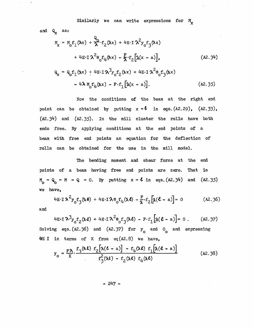
andSimilarly we can write expressions for

as:Q

Hx = M^CSoc) + ^ ' f 2( x) + <H3.I ,X2yo£3(*x)

+ ^ E - I ^ f ^ x ) - |-f2 [*(x “ a)],

Ox = V i ^ * ) t i+ E - i ' ^ 3 y 0 f 2 ( > x ) + ^ E - I ^ 2 0 o f 3 ( H x )

~ ^ W * * ) - F-fx[Xx " a)]- (A2.35)

(A2.3^)

Now the conditions of the beam at the right endpoint can be obtained by putting x =t in eqs.(A2.29), (A2.33)»(A2.3*0 and (A2.35). In the mill cluster the rolls have both ends free. By applying conditions at the end points of a beam with free end points an equation for the deflection of rolls can be obtained for the use in the. mill model.

The bending moment and shear force at the end points of a beam having free end points are zero. That is Mq = Qq = M = Q = 0. By putting x = £ in eqs. (A2.3^) and (A2.35)

Solving eqs. (A2.36) and (A2.37) for yQ and 0Q and expressing 4E I in terms of K from eq(A2.8) we have,

we have,

and4E-I*2yof3ft*) + - ~ f 2 [*(£ - a)]= 0 (A2.36)

^E’l7i3yof2(a-e) + kE-I/\ ZQ<f J M ) - - a)]= 0 . (A2.37)

- 2 k? -

andF*2 f2ft<)-f2 [ft(l - a)] - - a)]K f 2 ( U ) - f ^ t ) - f (-Xfc)

(A2.39)

Substituting these values for y , 0 and M = Q = 0 ino o o oeq.. (A2.29) and simplifying we can write an expression for y(x) as:

whereA = sinhX.&cosX a-cosh X(£ - a) - sinX&coshXa* cos M l - a), B = cosh^Xx-sinXx + sinhXx-cosXx,G = sinhX£ •[sinXa*cosh X (£ - a) - cosXa* sinhX ( C - a)J,D = sinX£*[sinhX a»cosX ( t - a) - coshXa. sin X(6 - a)[.

sinh^X£ - sin^X£1 •2«A«coshXx cosXx + B(G + D) (A2.40)

- 2 -8 -

♦ Xp /u n it length

q = ky

Fig.A2.1. Forces ac t ing on a beam.

Q

dx M +dM

Q + d Q

Fig. A2.2. Forces acting on an e lem ent of the beam.

- 2^9 -

APPENDIX 3.

Actuator Transfer Function Gains.

A3.1. Actuator integral rate constant k .

An average value of rack response to a 10 Vmaximum demand is + 1.5 divisions/sec. where the full scaledeflection of the actuators is rou^ily + 80 mm. correspondingto a + 5 divisions. The input of this block is in volts andthe output is in mm. If it is assumed that the actuatormovement varies linearly with input voltage, then the integralrate constant k is given by a

A3.2. The feedback position transducer constant k .A full scale movement of actuator is + 80 mm for

a full scale demand of + 10 V. Therefore k^ is given by

A3.3. Calculation of forward gain k to give two equal roots.The dead space time constant Ta is 0.1 sec.

(supplied by BSC). The characteristic equation of the closed loop actuator transfer function from eq.(5.1*0 is

(A3.1)

= Z.k

kf = = 0.125 V/mm (A3.2)

8(1 + s-Ta) + k-kakf = 0 (A3.3)

- 250 -

i. e.

a aFor equal roots,

4k* k k.

( A 3 »

_1T2a

which gives ,

a f = 0 (A3-5)

k = 4t k k-a a f(A3.6)

i. e.

k 4*0.1*2.4*0.125 8*^ ' (A3.7)Therefore the closed loop transfer function gfs) becomes,3#

(A3.8)g (s) = ______________ 8.33*2.4________a 0.1s2 + s + 8.33x2.4x0.125

200s + 10s + 25

8(1 + 0.2s)2

i.e. = 8 and = 0.2 .

By substituting these values in eq. (5.17) we have,

and Ca = [l 0]A = " 0 1 ‘ » K = ‘ o"a a-25 -10 i

_200_(A3.9)

- 251 -

APPENDIX 4.

Strip Dynamics.

A f.l. Derivation of the state space form of strip dynamics.

Let

and Cd = [l o] . (A*Kl)Ad =1 0 •

• A ■-c

_-a -b d

Therefore the strip transfer function can be written as

gd(s) = Cd(sl - Ad)-1Bd

0]. s + b l"•

-c

-a s_ _ d_s(s + b) + a

_ -c(s + b) + d 2s + bs + a

1 - d - bes b . a+ :— *s +

(A*K2)d - be d - be d - be

From eq. (5.22) we can write g^(s) in terms of time constant and time delay x as:

S a ( s ) =s2 + (“ + T,)s + 1

(A^.3)2 “ ’ v 2 Ad-

Now equating coefficients of eqs. (A*K2) and (A f.3) we have

2 d - be * (A*h 4)

- 252 -

x<Td 1 2 d - be *

1 b— + T = — ----2 Ad d - be

1 = d - be *By solving eqs. (A*f.to (Ak.7) for a,b,c and d we have

(A4.5)

(A4.6)

(A*f. 7)

a = b = T + 2T<1- X Td > b " X-Td '4-T, + X

c = — and d = -- ----T'Td

(A*K 8)

A*K2. Strip time constant and time delay.If a medium strip speed is considered, say 5 V s»

and the distance between the roll gap and the shapemeter is 1.75 then the time delay x is given by,

x - i J i - 0.3 5 s.

The strip time constant may be derived as:T _ J2. _ Distance between coiler and roll gap d V Strip speed= - ^ = 0.85 s .

By substituting these in eq.. (5.23) we have,

(A4.9)

(A4.10)

Ad = 0 1 • Bd = '-1.1765"

-6.7227 -6.8908_ 14.8295and

ca = L1 (A*hll)

- 253 -

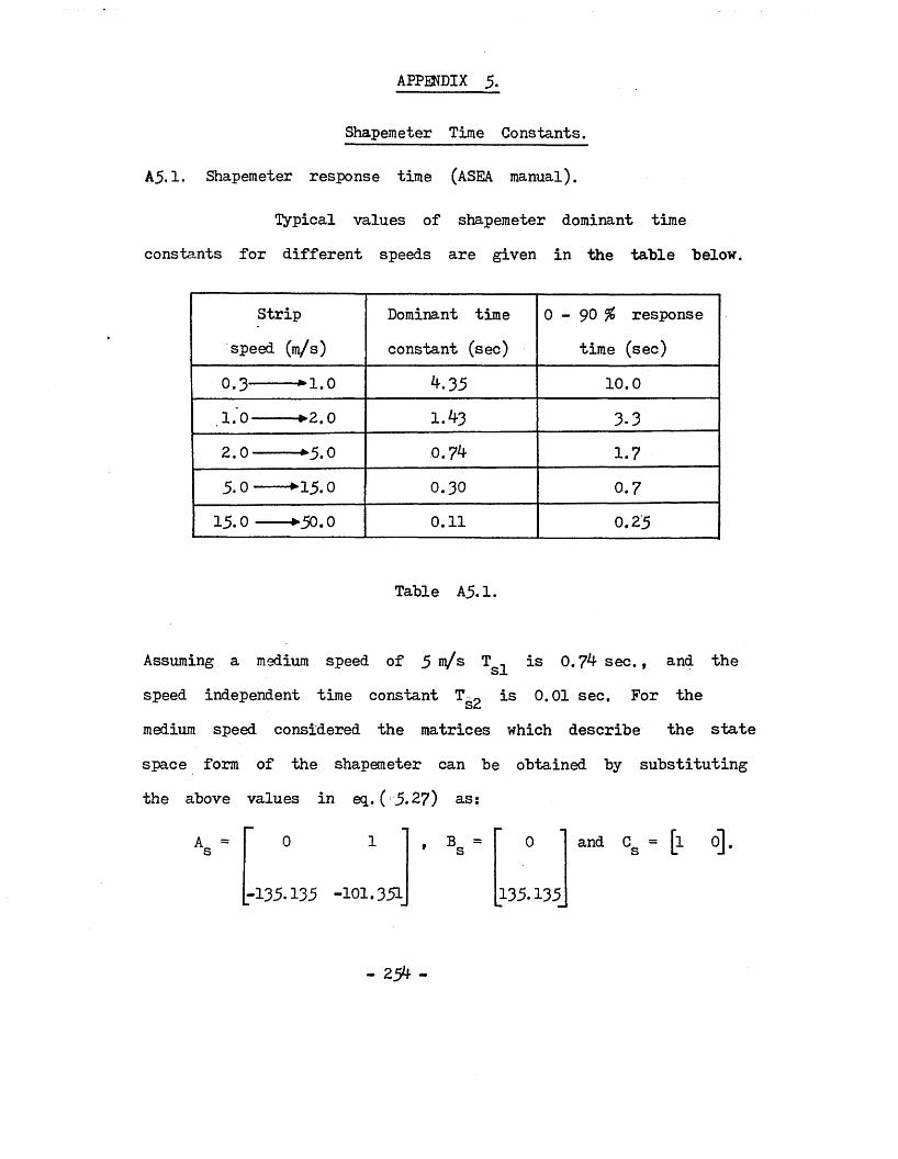
APPENDIX 5.

Shapemeter Time Constants.

A5.1. Shapemeter response time (ASEA manual).

Typical values of shapemeter dominant time constants for different speeds are given in the table below.

Strip speed (m/s)

Dominant time constant (sec)

0 - 90 % response time (sec)

0.3-----*1.0 4.35 10.01.0-----*2.0 1.43 3-32.0-----*5.0 0.74 1.75.0----*15.0 0.30 0.715.0--- *50.0 0.11 0.25

Table A5.1.

Assuming a medium speed of 5 V s is 0.74 sec., and thespeed independent time constant T^> is 0.01 sec. For the medium speed considered the matrices which describe the state space form of the shapemeter can be obtained by substituting the above values in eq.. ( 5.27) as:

As = 0 1 , Bs = [ 0 ] and Cs = [l o].0 1 f B = 0’ s

-135.135 -101.351 135.135_

- 2 5 4 -

APPENDIX 6.Mill Transfer Functions for Low, Medium

and High Speeds.

The • open loop mill transfer function has the form from eq.. (5.45),

For different speeds G(s) has different functions since the time constants depend on the speed. Assuming three different speeds, low, medium and high, the numerator and denominator polynomials, N(s) and D(s), are calculated and given below. The low, medium and high speeds used are 2.0 m/s, 5.0 m/s and 15.0 m/s respectively.

For low speed,N4(s) = 8 (1 - 0.4375s),

D (s) = (1 + 0.2s)2(l + 0.4375s)(1 + 2.125s)(lKf

+ l.43s)(l + 0.01s). (A5.1)For medium speed,

Nffl(s) = 8 (1 - 0.175s),

D (s) = (1 + 0.2s)2(1 + 0.175s)(l + 0.85s)(l+ 0.74s)(1 + 0.01s). (A5.2)

For high speed,Nh(s) = 8 (1 - 0.0583s),

D.(s) = (1 +0.2s)Z(l + 0.0583s) (1 + 0.283s)(l+ 0.3s)(l + 0.01s). (a5-3)

- 255 -

Appendix 7.

Yield Stress Curve for Stainless Steel Type 30 .

Fig.A7.1 shows (supplied by the manufacturer) the yield stress of stainless steel type 30^ plotted against the cold rolling percentage reduction. Data from this plot is used to calculate the yield stress atdifferent reductions, which is used in the roll forcemodel. This curve is modelled using a least square methodfor curve fitting, and a 6th order polynomial is derivedand is given by

y(r) = 229.819 + 29.0302r - 0.1l463^r2 - 0.03520l4aP

+ 0.00176116^ - 0.00003314-18IT5

+ 0.000000215601r6 (A7.l)

where y(r) is the yield strength in l^mm and r is the percentage reduction.

The numerical values from fig.A7.1 aretabulated in table A7.1 against the results obtained fromeq.(A7.1) and the third column shows the percentage errors.The relevent percentage reductions lie between 8 % and 26 % and the percentage error in this region is less than 2 %.

% reductionYield stress from fig.A7.1 in I0 nm2

Yield stress from eq.(A7.1)

in N/mrt?% error

0.0 233.33 229.82 -1.52.0 293.33 287.16 -2.1

4.0 333.33 342.27 2.76.0 386.67 394.30 2.0

8.0 440.00 442.88 0.710.0 480.00 487.96 1.712.0 520.00 529.76 1.914.0 560.00 568.63 1.516.0 600.00 605.05 0 .8

18.0 633.33 639.51 1.0

20.0 666.67 672.48 0.922.0 700.00 704.38 0.6

24.0 733.33 735.50 0.326.0 760.00 766.05 0.828.0 800.00 795.07 -0.530.0 820.00 825.48 0.732.0 850.67 854.07 0.434.0 877.33 881.52 0 .536.0 900.00 907.41 0 .8

38.0 922.67 931.28 0.94o.o 940.00 952.67 1.342.0 960.00 971.16 1.2

44.0 973.33 986.46 1.346.0 986.67 998.48 1.2

48.0 993.33 1007.39 1.450.0 1006.33 1013.71 0.752.0 1013.33 1018.66 0.554.0 1020.00 1023.17 0.356.0 1033.33 1031.31 -0.2

53.0 1040.00 1044.69 0.560.0 1053.33 1068.10 1.4

Table A7.1.

- 257 -

Yiel

d st

ress

in

N/m

m

1000.-

CNJ

600.-

200.

60.40. 50.30.2 0.10.0% Reduction

Fig.A7.1. Yield stress of stainless steel type 304.

- 258 -

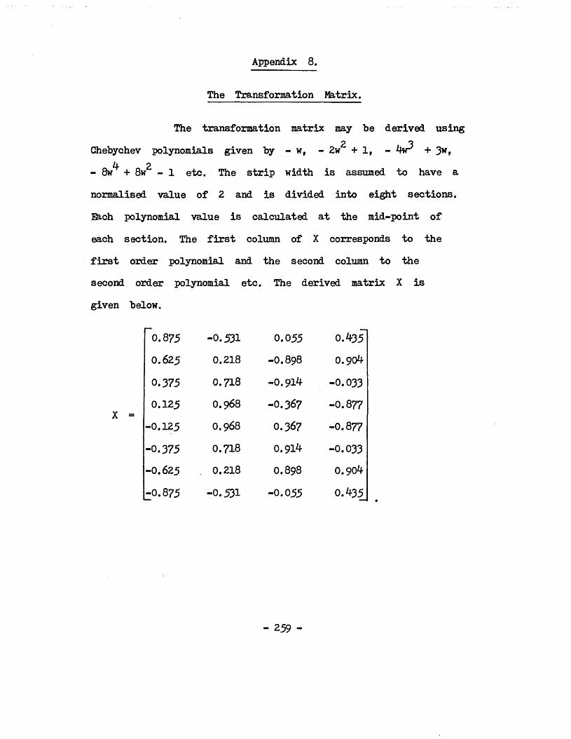
Appendix 8.

The Transformation Matrix.

The transformation matrix may be derived usingGhebychev polynomials given by - w, - 2w^ + 1,

L ?- 8w + 8w - 1 etc. The strip width is assumed to have anormalised value of 2 and is divided into eight sections.Ehch polynomial value is calculated at the mid-point of each section. The first column of X corresponds to thefirst order polynomial and the second column to thesecond order polynomial etc. The derived matrix X is given below.

0.875 -0.531 0.055 0.4350.625 0.218 -0.898 0.904

0.375 0.718 -0.914 -0.0330.125 0.968 -0.367 -0.877

-0.125 0.968 0.367 -0.877-0.375 0.718 0.914 -0.033-0.625 0.218 0.898 0.904

-0.875 -0.531 -0.055 0.435

- 259 -

Development of a Static Model for ASendzimir Cold Rolling Mill

G W D M GUNAWARDENE M J GRIMBLE Department of Electrical and Electronic Engineering

Sheffield City Polytechnic Pond Street Sheffield

Presented at:

IMACS (AICA) SYMPOSIUM ON

SIMULATION OF CONTROL SYSTEMS

with Special Emphasis on

MODELLING AND REDUNDANCY

September, 27 - 29, 1978

Technical University Vienna Austria

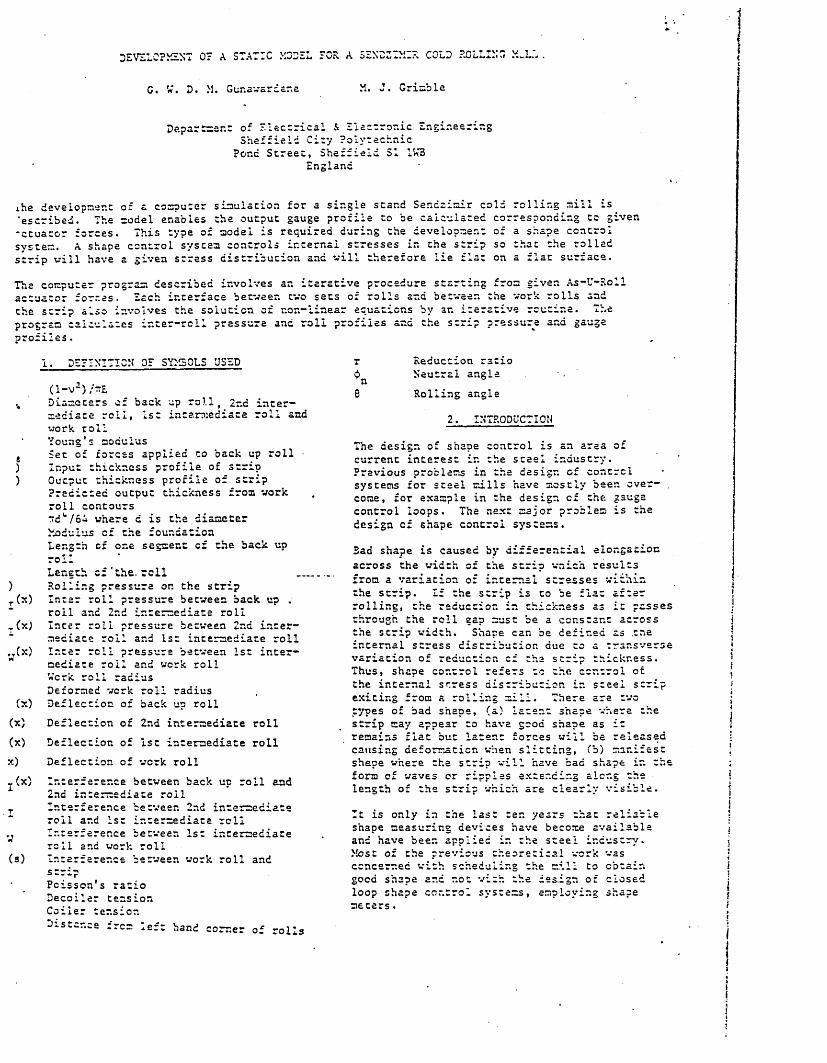
IDEVELOPMENT 07 A STATIC MODEL FOR A SENDZIMIR COLD ROLLING M^LL . j

IC. V. D. >J. Gunawardane M. J. Grimble

Department of Electrical & Electronic Engineering Sheffield City Polytechnic

Por.c Street, Sheffield SI LW3 Englanc

ihe development of a computer simulation for a single stand Sendzimir cold rolling mill is 'escribed. The model enables the output gauge profile to be calculated corresponding tc given -ctuacor forces. This type of model is required during the development of a shape control system. A shape control system controls internal stresses in the strip so that the rolled scrip will have a given stress distribution and vill therefore lie flat on a flat surface.

The computer program described involves an iterative procedure starting from given As-U-Roll actuator forces. Each interface between two sets of rolls and between the work rolls and the strip also involves the solution of non-linear equations by an iterative routine. The program calculates inter-roll pressure anc roll profiles and the strip pressure and gauge orofiles.

1. DEFINITION OF SYMBOLS USED

(l-va)/r£v Diameters of back up roll, 2nd inter­

mediate roll, 1st intermediate roll and work roll Young's modulus

8 Set of forces applied to back up roll •) Input thickness profile of strip) Output thickness profile of scrip

Predicted output thickness from work roll contours~du/6i where d is the diameterModulus of the foundationLength of one segment cf the back uproilLength cf'the. roll Rolling pressure on the strip

(x) Inter roll pressure between back up .roll and 2nd intermediate roll

(x) Incer roll pressure between 2nd inter­mediate roll and 1st intermediate roll

,(x) Incer roll pressure between 1st inter- 1 mediate roil and work roll

Work roll radius Deformed work roll radius Deflection of back up rollDeflection of 2nd intermediate rollDeflection of 1st intermediate rollDeflection of work rollInterference between back up roll and 2nd intermediate roil Interference between 2nd intermediate roil and 1st intermediate roll Interference between 1st intermediate roll and work roll Interference between work roll and stripPcisson's ratio Decoiler tension Coiler tensionDistance from left hand corner of rolls

r Reduction ratios>n Neutral angle6 Rolling angle

2. INTRODUCTION

The design of shape control is an area of current interest in the steel industry.Previous problems in the design of control systems for steel mills have mostly been over- . cone, for example in the design cf the gauge control loops. The next major problem is the design cf shape control systems.

Bad shape is caused by differential elongation across the width of the strip vnich results from a variation or internal stresses within the scrip. If the strip is to be flat after rolling, the reduction in thickness as it passesthrough the roll gap must be a constant across the strip width. Shape can be defined as tne internal stress distribution due to a transverse variation of reduction cf the strip thickness. Thus, shape control refers to the control of the internal stress distribution in steel strip exiting from a rolling mill. There are two types of bad shape, (a) latent shape where the strip nay appear to have good shape as it remains fiat but latent forces will be released causing deformation when slitting, fb) manifest shape where the strip will have bad shape in the form of waves or ripples extending along the length of the strip which are clearly visible.

It is only in the last ten years that reliable shape measuring devices have become available and have been applied in the steel industry.Most of the previous theoretical work was concerned with scheduling the mill to obtain good shape and not with the des.ign of closed loop shape control systems, employing shape meters.

0

/ S a c ! Up. R o tl

fmt«iOI» *SU

.:» • t n l « r m * 0i o t t R o ll

Figure 1

Sendzimir mill is & cluster mill (Fig 1) e c'ne work rolls rest between supporting s which permit the roll separating force e transmitted directly to the mill housing. ^ e are several types of Sendcinir mill buc he following the 1—2—3—4 mill will be icered as shown in figure 1. In this type ill there are eight backing shafts (numbered *

All bearing shafts are concentrically ted on roller bearings and are located .ntrically on saddles. This type of mill four drive rolls,- to which power is smitted through four large diameter .dies. Both work rolls are driven by the drive rolls through friction contacts with

2nd intermediate rolls. By rotating the ring shaft the position of the backing ring, with respect to the housing, can be nged to closely control the distance between work rolls. This is the basic concrol ement of a Sendzimir mill that permits ■ id parallel and extremely accurate itioning of the rolls.

s type of mill has the As-U-Rcll crown ■ustment control motorised through small raulic motors. This adjustment is provided shafts 2 and 3 acting simultaneously through ery small eccentric gear train. The •1ustment can be made under load and therefore . be changed while the mill is rolling.

e main objective of the project is to design •. closed loop concrol system for the Sendzimir 11, to control the shape of the strip, wever a mathematical model must first be veloped to represent the conditions within e mill cluster. This paper is only concerned th the development of this model. In the Ilowir.g the static model is presented which

represents the Sendzimir mill cluster and the conditions within the roll gap.

3. MODEL DESCRIPTION

The procedure for calculating the thickness profile for a given set of forces applied to the back up rolls is discussed in this section.A flow chart showing the basic procedure is given in figure 2. All the mathematical formulae are given in the appendix. For the present analysis the edge of the strip is ignored and the strip width is assumed to be the same as the length of the work rolls and this will be improved in due course. A simplified model was first developed which was based on the mill configuration shown in figure 3. This model can be modified to represent the system shown in figure 1. However for the present the simple configuration shown in figure 3 will be discussed.

BtrtKE C3SSTAKTS,

IM T tA L tS t h . ( i )

Binutcz * vtcro* r*a« u r r kjuo ;mo calculation

i m u t u u ocrucrioM tix u >.

_______Calculation[ l o l l Toner j ( , ) CALCULATION I

iW T s m n iN c * s e t v h s w l l • o il and s t x i* c alc vla -

M i ) • * {« )

J» l * ’ . n_cv c a s t ro x t m s a il r to c iA n

3

Back Up Roll

emediate Roll

D—«}lst Intermediate RollWork Roll u_n.

v

Figure 3

INITIAL ROLL DEFLECTION AND PRESSURE DISTx.i3Li ..ON CALuULAi *.0N

icial roll deflections y=rr„(x), y (x), and v„(x) due to a sec of applied* Ware calculated using bean choery for g. For the present analysis the tions due to shear components are ignored, "s justified because the rolls with free ave no shear bending and the span/depth is very high. The left and right end s of all the rolls are free and hence the t and shear at these points are zero.

the deflection of cile back updue to a set of forces F is calculated, ing that it is resting on the 2nd inter- te roll.' As the back up roll is pressed st the 2nd intermediate roll, by the ed force, this results in a set of reaction, s between the back up roll and the 2nd jediate roll. This pressure distribution noted by RB2I^X' ar* ca^cu^ate^ usingquations (1), (5) and (6) in appendix 1.

farces acting at the point of contact of oack up roll and 2nd intermediate roll, e a set of forces equal and opposite to (x), acting on the 2nd intermediate roll.sec of forces can be considered as the es acting on the 2nd intermediate roll, deflection of the 2nd intermediate, due to the pressure q (x) is thenulated (assuming the 2nd intermediate roll esting on the 1st intermediate roll). This ection will cause the 2nd intermediate roll ress against the 1st intermediate roll, rating another pressure profile, which is •Ced q21I(x)‘larly the pressure orofile a.2il^ accs on1st-intermediate roll causing it to bend, deflection of the 1st intermediate roll is ted y^j(x). Clearly this deflection wille the generation of another pressure profile

q-,_(x) between the 1st intermediate roll and Zi.1the work roll. Finally the deflection }\»(x)4 wof the work roll, due to this pressure, iscalculated.

5. ROLLING PRESSURE CALCULATION

An extensive literature exists on the calculation of the specific roll force as a function of entry and exit thickness and tensions. The rolling force is calculated by dividing the strip into a number of sections (in this analysis 10). Within each section all the parameters are assumed to be constant. The arc of contact is assumed to be circular for this simple model.

When calculating rolling force a correction must be made to allow for the affect of roll flattening. This is achieved using Hitchcock's formula together with an iterative solution procedure. The solution is obtained when theroll radius error R' - R' ,n n-1

R'n

is less than a

given value, for example 17. (R' is the--new roll radius).

6. INTFR ROLL PRESSURE DISTRIBUTION CALCULATION

The inter roll pressure distributions q_„T (x),q„,_(x) and q. _,,(x) are calculated from the Zlx llwdegree of interferences between the back up roll and 2nd intermediate roll, 2nd and 1st inter­mediate rolls, and 1st intermediate roll and work rolls respectively. These inter roll pressures must satisfy the force equilibrium criteria for all the rolls, that is

/p(x)dx - /qlly(x)1IW 21]

/q (x)dx « Jq (x)dx211 /qs2I<*)*c

321 Er

(a)(b)(c)(d)

(1)

If minor bending distortions are ignored the roll surfaces can be assumed to be circular. When two infinitely long elastic cylinders are in contact the total interference between cylinders y can be written as a function of the load per unit length q.

A . r /e Oj +Dj) ty - q(ci +c:)loge . • Je ,;j ' > <2J

Th<* interference between rolls can be calculated from the roll contours yi and yz using the relation (figure 4)

7 i2 (x) - y 2 (x) - yi(x) + y:2 (0) (3)The method of calculating q(x) is to sub­stitute y-.2 (x) calculated frcn equation (3) for y in equation (2) and to adjust y i 2(0 )

tively until a solution to equations (1) 2) is obtained. This procedure has to be ted three tir.es to calculate the three ure profiles by substituting the . priate variables.

Figure ACALCULATION OF NEW ROLL DEFLECTIONSBUR (x), y?I(x), y1I(x),and yy (x)

ew deflections due to the inter rollure profiles are calculated in thewing manner. Consider one particular roll.are forces acting upwards and downwards

e roll. The deflection of the roll due e downward forces and due to the upward s are calculated in chat order. The erence between the two deflections is lated to give the total deflection of the The deflection due to the downward

es is taken to be positive and that due he upward forces is taken to be negative.

INTERFERENCE BETWEEN WORK ROLL AND STRIP

an elastic cylinder is resting on a flat ace the interference y can be written as

3 /.. 2 ,.O ' (A) (ref 1)rVe*Di.• 2?Cll:,se{-2ZTF

e p is the pressure applied. When __ulatir.g the interference between work roll the strip, the work roll can be considered cylinder resting on a flat surface. First 11 the pressure at the roll gap is ulated using the roll gap model. Then the sure p(x) is substituted in equation (A) ive the interference yWg(x) between Che workand the scrip as a function of x.

. PREDICTION OF THE NEW STRIP THICKNESS

variables given below are defined in ure 5.

x)X)(s)

(s)

(X)

(X)

(X)

Input thickness Output thickness Deflection of the measured from the Deflection of the measured from the Distance from the the upper side of Distance from the the lower side of Distance from the the upper side of

upper work roll mill housing lower work roll •mill housing mill housing to strip entering mill housing to strip entering mill housing to strip exiting

h2LW ■ Distance from the mill housing to the lower side of strip entering

hi(x) » h1T (x) - ^^(x)

h2L(x) ' h2U<X>

'WSU

h2(x)

(x) and * Interference between the work roll

W x>and the scrip due to flattening calculated from Hertzian expression referring to upper and and lower halves respectively.

h2u(x) ■ W x) - ywsu<*)h2L(x) - * W X>h2(x) ■ h2L(x) - h2a(x)

- y^Cs) - y^Cx) * yWSL(x)

+ ywsu(x)If we assume that the system is symmetrical about the centreline of the strip, then

W x) ■ W x)Therefore the predicted thickness is given by the affective work roll deflections plus the flattening, thus

H(x) yWL(=° • yWU(s) * 2yWSCx)Therefore the new estimate of strip thickness is found by substituting this expression for H(x) in the equation given below.

h*(x) - hk”1(x) + afH(x)-hK"i(x)J _k-1,

where a is a convergence parameter selected to obtain a stable solution.

Strip

Entry thickness orcfile Exit thickness profile Work roll profile

Figure 5

r

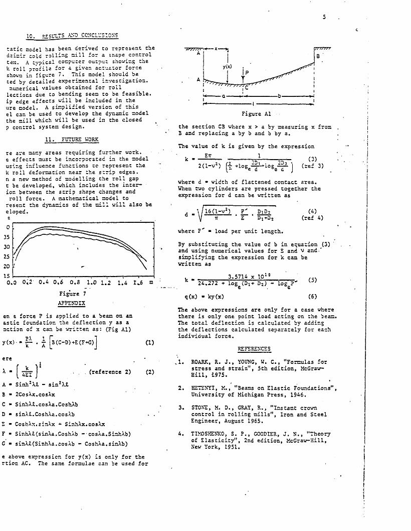
5

10. ?£SKLTS AND CONCLUSIONS

tatic model has been derived Co represent the dzimir cold rolling mi 11 for a shape control tem. A tvpicai computer output showing the k roll profile for a given actuator force shown in figure 7. This model should be ted by detailed experimental investigation, numerical values obtained for roll lections due to bending seem to be feasible, ip edge effects will be included in the ure model. A simplified version of this el can be used to develop the dynamic model the mill which will be used in the closed p control system design.

11. FUTURE WORK

re are many areas requiring further work, e effects must be incorporated in the model using influence functions to represent the k roll deformation near the strip edges, n a new method of modelling the roll gap t be developed, which includes the inter­ior. between the strip shape changes and roll force. A mathematical model to

resent the dynamics of the mill will also be eloped, a

0.0 0,2 0.4 0.$ 0.8 1.0 1.2 1.4 1*6 m

Figure 7 APPENDIX

en a force ? is applied to a beam on an astic foundation the deflection y as a nction of x can be written as: (Fig Al)

y(x) ' " IT * I [s(C-D)+E(F+G)J ere

f - M *. 4EI JX •

A ■ Sinh2Xi - sin2X&

(reference 2)

(1)

(2)

B * 2CosXx.cosAxC » SinhXJl.cosAa.CcshAbD • sinXi.CoshXa.cosXbE ” CoshXx.sinXx * SinhXx.cosXxF ■ SinhXZ(sinXa.CoshXb -•cosXa.SinhXb)G ■ sinX2(SinhXa.cosXb - CoshXa.sinXb)

e above expression for y(x) is only for the rtion AC. The same formulae can be used for

y(x)

Figure Al

the section CB where x > a by measuring x from B and replacing a by b and b by a.

The value of k is given by the expression S7T 1k - ---------- rr--rr— (3)2U-v*> +i0gei 2 U i0gei|2. j (ref 3)

where d - width of flattened contact area.When two cylinders are pressed together the expression for d can be written as

d - / 16( l - v 2) . I l .\j u E Dj+Dawhere F" ■ load per unit length.

(4) (ref 4)

By substituting the value of b in equation (3) and using numerical values for E and v and-* simplifying the expression for k can be written as

k - 3.5714 x 10:o24.272 ♦ log (Dj+ Da) - log ?'e e

q(x) - ky(x)

(5)

(6)The above expressions are only for a case where there is only one point load acting on the beam. The total deflection is calculated by adding the deflections calculated separately for each individual force.

REFERENCES

1. ROARK, R. J., YOUNG, W. C., "Formulas for stress and strain", 5th edition, McGraw- Hill, 1975.

2. HE7ENYI, M., "Beams on Elastic Foundations", University of Michigan Press, 1946.

3. STONE, M. D., GRAY, R., "Instant crown control in rolling mills", Iron and Steel Engineer, August 1965.

4. TIMOSHENKO, S. P., G00DIER, J. N., "Theory of Elasticity", 2nd edition, McGraw-Hill,New York, 1951.

GRIM3LZ M. J*» roll force model for the cold rolling of chin sheer", Industrial Autonation Group Report 4/74, Imperial College Science and Technology, April 1974.

GRIM3LE, M. -•i "Shape control for rolled strip", >*ech Eng, Nov 1975, pp 91-93.

GRIMBLE, M. J., "A roll force model for tin- - plate rolling", GEC J of Science and Technology, Vol 23, No 1, 1976, pp,3-12.

GRIMBLE, M. J., FULLER, M. A., BRYANT, G. F. "A non-circular arc roll force model for cold rolling", International J for Numerical- Methods in Engineering, Vol 12, 1978, pp 643-663.

BRAVINGTCN, C. A. 3ARRY, D. C., McCLURE C.H. "Design and development of a shape control system", Shape Control Confr, Metal Society, Chester, Mar 1976.-

CONTE, S. D., "Elementary Numerical Analysis", McGraw-Hill, 1965.

EDWARDS, W. J., SPOONER, P. D., "Analysis of strip shape", in Automation of Tandem Mills edited by G. F. 3ryant, pub Iron and Steel Inst, 1973, pp 177-212.

KARACUCHI, S., KAJIWARA, T., HATA, K.,"Shape of scrip steel in cold rolling process", Bulletin of the ISME, No 67,Jan 1971, pp 104-112.

OROWAN, E., Proc IME, 1943, Vol 150.

SABATINI, 3., YEOMANS,*K. A., "An algebra of strip shape and its application to mill scheduling", J of the Iron and Steel Inst, Dec 1968m pp 1207-1217.

SAXL, K., "Transverse gauge variation in strip and sheet rolling", Proc of Inst of Mech Eng, Vol 172, No 22, 1953, pp 727-742.

SPOONER, ?. D., BRYANT, G. F., "Analysis of shape and discussion of problems of scheduling set-up and shape control", Shape Control Conf Proc, Metal Society, Chester Mar 1976, pp 19-29.

UNDERWOOD, L. R., "The Rolling of Metals Theory and Experiment", Vcl 1, Chapman &Hall Ltd, London 1950.

ACKNOWLEDGEMENTS

The authors would like to acknowledge the contributions to the project by Dr G F Raggett of the Department of Mathematics and Statistics, Sheffield City Polytechnic and Mr M Foster of the Svinden Laboratories of 3ritish Steel Corporation.

Reprinted from

TECHNOLOGYA PUBLICATION OF THE METALS SOCIETY

THE METALS SOCIETY 1 CARLTON HOUSE TERRACE LONDON SW1Y 5DB

Static model for Sendzimir cold-rolling mill

G. W. D. M. Gunawardene M. J. Grimble A. Thomson

The design of shape-controlsystems is an area of current interest in the steel industry. The object of shape control is to adjust the mill so that the rolled strip is free from internal stresses. Both static and dynamic mill models are required for this purpose.A static model enables shape profiles to be calculated for a given set of actuator positions, and is used to generate the steady-state mill gains. Such a model is presented in this paper. The method of calculation of shape profiles is discussed.These shape profiles are plotted against the distance across the strip. Linearized mill gains are calculated about a given shape-operating point and these relate the shape changes to the actuator changes. A mill gain matrix, obtained by measuring shape at eight points across the strip, is presented. MT/699

© 1981 The Metals Society. Manuscript received 11 January 198 . G. W. D. M. Gunawardene is in the Department of Electrical and Electronic Engineering, Robert Gordon's Institute of Technology, Aberdeen, Dr Grimble is in the Department of Electrical and Electronic Engineering, Sheffield City Polytechnic, Sheffield, and Dr Thomson is with GEC Electrical Projects Ltd, Rugby.

List o f symbols

C = (l — constant, m2N </i=diameter of roll 1 when two rolls are pressed to­

gether, mdz= diameter of roll 2 when two rolls are pressed to­

gether, mE = Young’s modulus of the material, N m-2 F= total force applied, N

Gm=gain matrix (shape change to rack change) /n(x)=input-thickness profile, m /»2(x)=output-thickness profile, m J /j2=mean change in gauge profile, m

Ahzix) = deviation of gauge profile from mean, m 4//2'(*)=change in gauge profile, m

/=7«/4/64, m4A'=elastic-foundation constant, N m-2 k= mean yield stress, N m-2 ki =entry yield stress, Nm -2 &2=exit yield stress, Nm -2 N=no. of sections across mill width

p(x)=specific rolling force, N m-1 =mean rolling force, N m-1

q{x)= inter-roll specific pressure between two rolls, N m-1 7?=work-roIl radius, m

7?'=deformed roll radius, m w'=work-ro!l width, m 1^= width of strip, m.r=distancefrom left-hand corner of mill or roll, m

y(x)= deflection of any roll, m j s(x)=deflection of upper roll, m yt(x)=deflection of lower work roll, m

ywc(x) = work-roll camber, m >Vs(a:) interference between work roll and strip, m >5ws(x)=mean interference between work roll and strip, m yi(x)=deflection of roll 1 when two rolls are pressed to­

gether, mj 2(x)=deflection of roll 2 when two rolls are pressed to­

gether, m>>i2(a:) interference between two rolls pressed together, m

a=output stress-convergence parameter /?=stress-equation constant

y= ratio of input-output deviation 8=/n(x)— /*2(;c)=amount of reduction, m H=coefficient of friction v=Poisson’s ratio

cti(x) in p u t tensile stress, N m-2 o2(x)=output tensile stress, Nm -2

Aoo(x)=input tensile stress deviation of first pass, N/m-2 Aaz(x)=output tensile stress deviation from mean, N/m -2

<f>n=neutral angle

The design of shape-control systems is an area of current interest1-4 in the steel industry. Previous problems in the design of control systems for steel mills have been over­come largely, for example, in the design of gauge-control loops. The next major problem involves the design of shape-control systems. Shape control refers to the control of the internal-stress distribution in steel strip leaving a roll­ing mill.5-6 It is only in the last ten years that reliable shape- measuring devices have become available and have been applied in the steel industry.

To illustrate how bad strip shape might arise, consider strip having a uniform input thickness and a work roll which is deformed so that the output strip thickness is greater near the strip edges than in the central region. In the absence of lateral spread the strip must be larger in the central region than at the edges. Since the strip is one homogeneous mass, such differential elongations cannot occur and internal stresses result. Clearly, if the strip is to be flat after rolling the reduction in thickness, as it passes through the roll gap, must be constant across the strip width.

Shape may be defined as the internal-stress distribution owing to a transverse variation of reduction of the strip thickness. There are two types of bad shape: (a) a latent shape where the strip may appear to have good shape in the mill under tension, but where bad shape is evident during slitting operations, and (b) a manifest shape where the strip being rolled has bad shape in the form of waves and ripples, extending along the length of the strip, which are clearly visible, see Fig.l. The stress distributions associ­ated with these basic defects are illustrated in Fig.2.

The first requirement in the analytical design of a shape- control system is for the development of a model of the

274 Metals Technology July 1981

Gunawardene et al. Model for Sendzimir mill 275

(a)

(b)a la ten t shape on subsequent s litting a lon g m idd le or long e d g e ; b m anifest shape w ith lo n g edges

1 Various form s o f shape defect

rolling mill. Both static and dynamic mill models are re­quired. A static model enables shape profiles to be calcu­lated for a given set of actuator positions and it is used to generate the steady-state mill gains. The dynamic model represents the dynamic performance of all the mill com­ponents, such as the actuators, and is based upon the equations of state for the system. The subject of this paper is the static model for a Sendzimir cold-rolling mill.7-8 A Sendzimir mill is extremely complex mechanically, as may be seen from the roll configuration in Fig.3. There has been little published work on the development of such models for this type of mill.

3 Sendzim ir m ill roll cluster

Description o f mill

GENERALThe Sendzimir mill (Z mill) to be considered here is l -7 m wide and is a cluster mill where the work rolls rest between supporting rolls. The mill has eight backing shafts labelled A-H, six second intermediate rolls (I-N), four first inter­mediate rolls (O-R), and two work rolls (5, T), as shown in Fig.3. This type of mill is used for rolling hard materials such as stainless steel.

The motor drive is applied to the outer second inter­mediate rolls (/, K, L, N) and the transmission of the drive to the work rolls via the first intermediate rolls is due purely to inter-roll friction. Rolls labelled l-T have free ends and are free to float. The outer rolls (A-H) are split into seven roll segments, as shown in Fig.4. The shafts in which these rotate are supported by eight saddles per shaft, positioned between each pair of roll segments and at the shaft ends. The saddles are fixed rigidly to the mill housing, and con­tain eccentric rings. The outer circumferences of these rings are free to rotate in the circular saddle bores, while the inner circumferences are keyed to the shafts.

a long e d g e , b long m id d le ; c h e rrin g b o n e ; c/quarter buckle

2 Stress distributions and m anifest buckling form s

saddles boltedto mill housing

shaft

saddles

roll segmentseccentric ring in each saddle (keyed to shaft)

(backing bearings) arc free to rotate on shaft

4 Backing sh aft assembly, shafts A and D-H

Metals Technology July 1981

276 Gunawardene et al. Model for Sendzimir mill

mill housingbacking bearing

saddleAs-U-Roll eccentric ring

screwdown eccentric ring

shaft

roller bearings at these two interfaces

'parallel'circular loci of C2 and C3 due to indicated rotation of As-U-Roll ring only

5 Saddle detail fo r shafts B and C (n o t to scale)

UPPER AND LOWER SCREWDOWN OPERATIONOperation of upper screwdown racks acts on assemblies B and C, and assemblies F and G are responsible for the lower screwup system. Each saddle of the assembly Band C is constructed as shown in Fig.5. The saddles on the Band G assembly are also constructed in the same way but without the ‘As-U-Roll’ eccentric rings.* When the shaft is rotated the eccentric screwdown ring also rotates in the saddle bore, since it is keyed to the shaft. This allows the centre cz of the shaft to rotate about the centre ci of the saddle bore, thus causing a net movement of the shaft to­wards or away from the mill housing. Since the shaft is keyed to the screwdown eccentric rings in all eight saddles the same motion will occur at each end and the shaft will remain parallel to the mill housing. Essentially, the screwdowns cause the movement of rolls /, J, K, O, P, and S up or down which enables the distance between the two work rolls to be adjusted finely during rolling. A similar operation, which is used principally for roll chang­ing and mill threading, takes place at the lower assemblies Band G.

'AS-U-ROLL' OPERATIONIn addition to the screwdown system, each of the saddles

♦These are made by the Sendzimir Company; they allow roll bending to take place during rolling to adjust strip shape.

second intermediate roll

first intermediate rollwork roll

a. □ x0 . Q D , G, □

second intermediate roll

first intermediate rollwork roll

a racks before m o tio n ; b racks a fter m otion

7 Example of A s-U -Roll action

supporting the upper shaft assemblies B and C is fitted with an extra eccentric ring (Fig.5) situated between the saddle and the screwdown eccentric ring. This eccentric ring can be rotated independently of the shaft and screwdown eccen­tric ring, by moving a rack which operates on two annular cheeks fitted on each side of this extra ring, as shown in Fig.6. Such rotation will cause the centre C3 of the inner bore of this ring to move in a circular locus about centre ci. There are eight such As-U-Roll racks on saddles between segments. These racks are capable of individual adjustment, producing a different displacement between the shafts and the housing at each saddle position. This allows a profile to be forced on to the shaft, as shown in Fig.7, which will propagate to the work roll through the cluster. Although the As-U-Rolis and upper screwdowns act on the same common shaft they are essentially non-interactive.

P

first intermediate roll with tapered end

front

millstrip

work roll

work roll

6 A s-U -R oll assembly

first intermediate roll with tapered end

8 Tapered firs t interm ediate rolls

Metals Technology July 1981

Gunawardene et at. Model for Sendzimir mill 277

FIRST INTERMEDIATE ROLL TAPERS In addition to As-U-Roll control of strip shape there is another type of control on the Z-mill. The first inter­mediate rolls O-R are furnished with tapered-off ends, see Fig.8. These rolls can be moved laterally in and out of the cluster. The top and bottom rolls may be moved indepen­dently, and it is thus possible to control the pressure at the edges of the strip within certain limits. These rolls are, therefore, used to control the stresses at the edge of the strip.

Static model fo r m ill

at that point.10 In the mill all the rolls in the middle of the cluster are resting on one another and, since these rolls are elastic bodies, it can be assumed that each roll is resting on an elastic foundation. Thus, the actual bending deflections y can be calculated (see Appendix 1) as a function of the applied force F and the distance x from one end of the beam, i.e.y=f(F,x)........................................................................(1)

Roll fla tten ing and in ter-ro ll pressure distribution

A static model7 for the single-stand cold-rolling mill, shown in Fig.3, may now be described. The static model is a mechanical model for the mill which represents all force- deformation relationships in the roll cluster and in the roll gap. It is important for control purposes to note that these relationships are very non-linear and schedule dependent.

The static model must allow for the bending and flatten­ing of the rolls in the cluster and for the plastic deformation of the strip in the roll gap. The model must provide:

(i) linearized mill gains for use in the control system simulation (dynamic model) based upon a small perturbation analysis

(ii) an understanding of the way in which shape is affected by the mill actuators

(iii) details of the range of control which is available using the As-U-Roll or the first intermediate roll tapers.

The assumptions made in deriving the static model may be listed as:

(i) the mill is symmetrical about a line passing through the work-roll centres (this need not be the case if the side eccentrics are set differently)

(ii) strip edge effects may be ignored(iii) deflections due to shear may be neglected(iv) elastic recovery of the strip may be neglected(v) horizontal deflections of rolls may be neglected

(vi) the centreline strip thickness is specified.The model developed is in the form of a Fortran computer program. The model enables the output shape profile to be calculated corresponding to a given set of rack positions. The model is divided into three main sections, namely:

(i) roll bending: for calculating the roll-bending de­flections due to a set of forces

(ii) roll flattening: for calculating the roll interference or roll flattening between two rolls forced together

(iii) roll force: for calculating the rolling force required to reduce the thickness of the strip by a given amount

(iv) gauge and shape: for calculating the output gauge and shape profiles corresponding to a given set of inter-roll pressure and deflection profiles.

The above topics are considered in the sections below.

Roll bending

It is well known that if a force is applied to a beam9 sup­ported at two ends, the reactions at the ends and the de­flection of the beam can be calculated using simple bendingtheory. If the beam is resting upon an elastic foundation, where the whole length of the beam is in contact with the foundation, the deflection of the beam may be calculated by assuming that the deflection is proportional to the reaction

The effect of roll flattening, u >12 and the resulting inter-roll pressure distribution, is considered in this section. Recall that when two elastic cylinders are rolled together under a load F, the roll axes are deflected. The roll surface of contact will also be flattened.

The amount of interference, or the flattening yiz(x) be­tween the rolls, can be calculated as a function of the inter­roll specific force g(x). Alternatively, q(x) can be calculated as a function of yiz(x) :yiz(x)=U(q(x))...............................................................(2)?C*)=f2(yi2(*))...................(3)

The interference can also be calculated using the roll con­tours due to bending. This is a function of the deflections yi(x) and y2(x) of the two rolls.yiz(x)= f 3(yi(*), y2(x)) ........... (4)

The full expressions are given in Appendix 2.The deflections yi(x) and j>2(a:), clearly, will depend upon

the pressure q(x) and, hence, on yiz(x). From equation (3) it may be seen that q(x) depends on y i2(;c) and, hence, q(x) and y i2(x) must be calculated iteratively. The total pressure across the roll width must be equal to the applied force F for the system to be in equilibrium, i.e.

f q(x)dx=F.................................................................. (5)J 0

The method of calculating q(x) is to substitute for y i2(;c) in equation (3) from equation (4) and to solve equations (3) and (4) iteratively by changing the distance between the roll centres until equation (5) is satisfied to within a specified tolerance. The interference between the work roll and the strip is calculated in a similar manner (see Appendix 2).

Roll-force model

The amount of reduction in thickness of the strip is related to the total load in the mill or roll force.13-15 Extensive literature exists on the calculation of specific rolling force p(x) as a function of input-output thicknesses, input- output tensions, and work-roll radius.16p(x)=f(hi(x), hz(x), oi(x), <rz(x), R) .............................. (6)

When rolling hard materials like stainless steel, very high forces must be applied. Since the work rolls are elastic bodies, they will be deformed and flattened at the roll gap.17 In order to calculate the roll force, including the flattening effects, an iterative procedure must be adopted because the deformed roll radius is a function of the roll force. The deformed radius R' can be calculated using Hitchcock's formula, given as

(7)

Metals Technology July 1981

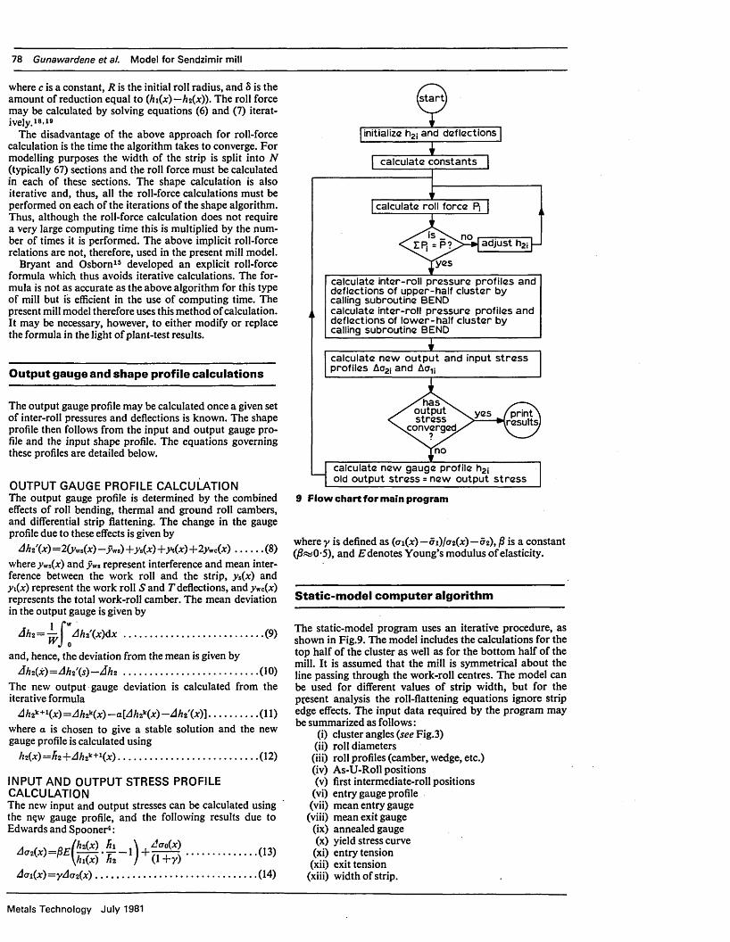
78 Gunawardene et al. Model for Sendzimir mill

where c is a constant, R is the initial roll radius, and 8 is the amount of reduction equal to (hi(x)— hi(x)). The roll force may be calculated by solving equations (6) and (7) iterat­ively.18-19

The disadvantage of the above approach for roll-force calculation is the time the algorithm takes to converge. For modelling purposes the width of the strip is split into N (typically 67) sections and the roll force must be calculated in each of these sections. The shape calculation is also iterative and, thus, all the roll-force calculations must be performed on each of the iterations of the shape algorithm. Thus, although the roll-force calculation does not require a very large computing time this is multiplied by the num­ber of times it is performed. The above implicit roll-force relations are not, therefore, used in the present mill model.

Bryant and Osborn15 developed an explicit roll-force formula which thus avoids iterative calculations. The for­mula is not as accurate as the above algorithm for this type of mill but is efficient in the use of computing time. The present mill model therefore uses this method of calculation. It may be necessary, however, to either modify or replace the formula in the light of plant-test results.

O utput gauge and shape profile calculations

The output gauge profile may be calculated once a given set of inter-roll pressures and deflections is known. The shape profile then follows from the input and output gauge pro­file and the input shape profile. The equations governing these profiles are detailed below.

OUTPUT GAUGE PROFILE CALCULATION The output gauge profile is determined by the combined effects of roll bending, thermal and ground roll cambers, and differential strip flattening. The change in the gauge profile due to these effects is given byAhz'(x)=2(yws(x) —yW8) + ys(*) +2y*c(x)..........(8)

where yWs(x) and yws represent interference and mean inter­ference between the work roll and the strip, ys(x) and y\(x) represent the work roll S and T deflections, and y«c(x) represents the total work-roll camber. The mean deviation in the output gauge is given by

Ah2=jyjWAh2'(x)dx.................................................. (9)

and, hence, the deviation from the mean is given byAh2{x)=Ah2'(s)-Ah2 ................................................(10)

The new output gauge deviation is calculated from the iterative formulaAhzk+Kx) =AhzKx)- a[AhzKx)-Ahz'ix)]..................(11)

where a is chosen to give a stable solution and the new gauge profile is calculated using

h2(x)=fi2+Ah2k+1(x).................(12)INPUT AND OUTPUT STRESS PROFILE CALCULATIONThe new input and output stresses can be calculated using the n$w gauge profile, and the following results due to Edwards and Spooner4:

«■>Acn(x)=yA<72(x).......................................................... (14)

start

noIP: =P?

yes

yes

no

X h a s X output ^ stress

converged,

adjust h2j

( print A ircsultsj

calculate constants

calculate roll force

initialize h2i and deflections

calculate new gauge profile h2jold output stress = new output stress

calculate new output and input stress profiles Ao2i and Ao^

calculate inter-roll pressure profiles and deflections of upper-half cluster by calling subroutine BEND calculate inter-roll pressure profiles and deflections of lower-half cluster by calling subroutine BEND

9 Flow chart fo r main program

where y is defined as (ai(x)—5i)/o2(x)— 02), jS is a constant (jSssO-5), and E denotes Young’s modulus of elasticity.

Static-m odel com puter algorithm

The static-model program uses an iterative procedure, as shown in Fig.9. The model includes the calculations for the top half of the cluster as well as for the bottom half of the mill. It is assumed that the mill is symmetrical about the line passing through the work-roll centres. The model can be used for different values of strip width, but for the present analysis the roll-flattening equations ignore strip edge effects. The input data required by the program may be summarized as follows:

(i) cluster angles {see Fig.3)(ii) roll diameters(iii) roll profiles (camber, wedge, etc.)(iv) As-U-Roll positions(v) first intermediate-roll positions

(vi) entry gauge profile(vii) mean entry gauge

(viii) mean exit gauge(ix) annealed gauge(x) yield stress curve(xi) entry tension

(xii) exit tension(xiii) width of strip.

Metals Technology July 1981

Gunawardene et at. Model for Sendzimir mill 279

exit enter

10 Path o f calculation for subroutine BEND to calcu­late pressure profiles

The output data may be listed as:(i) inter-roll pressure (12 profiles)

(ii) roll deflections (12 profiles)(iii) exit shape (stress-distribution) profile(iv) exit gauge profile(v) roll-force profile.

The mill width is divided into a number of section mul­tiples of 67 and the following assumptions are made (the number 67 is chosen to match the dimensions of the back­up roll and its segments):

(i) the pressure distribution in each section may be cal­culated using a point load applied at the centre of the section and the width of the section

(ii) the mean deflection of a roll over a section is taken to be equal to the deflection at the centre of the section.

(enter

new q(x)= old q(x)?

no

yes

exit

calculate q(x)

initialize q(x)

old q(x) = new(x)

adjust distance between two roll centres

calculate deflections y1 and y2 of rolls 1 and 2 using q(x)

calculate interference between rolls 1 and 2 using y1 and y2

11 Flow chart for calculating inter-roll pressure be­tween tw o rolls

36 rack 1—x— rack 224

-24

Ixi -36

-60racks land 2 1mm change 1-6W

-72X DISTANCE

12 Shape profile for 1 mm change in racks 1 and 2

This principle also applies to the stress distribution, strip profile, roll-pressure profile, etc. The computer algorithm enables a change in the shape profile owing to a change in the rack position, and hence the gains of the mill, to be calculated. The flow chart for the main program is shown in Fig.9.

The program begins by initializing all the variables, and the roll force is then calculated using the roll-gap model. Symmetry about a line passing through the work-roll centres can be assumed so that calculations are necessary only for the left side of the cluster. The subroutine BEND calculates the pressure profiles and roll profiles of one half of either the top or bottom cluster. I f symmetry is not as­sumed then the routine BEND has to be called four times to calculate all the pressure and roll profiles. At the end of each iteration a convergence test is carried out on the shape profile. The above calculations are repeated until the error between two successive shape profiles is less than a pre­determined value.

The pressure and roll-profile calculation procedure is illustrated in Fig. 10. Only the top-half cluster is shown in this figure and thick lines are drawn to show the path of calculation. The small circles labelled ci, cz, C3, and c\ re­present an iterative process for a particular inter-roll pres­sure calculation. A satisfactory convergence in pressure is shown by Yand non-convergence is represented by N.

As the pressure profile between two rolls depends on the . interference or flattening of the rolls, and the interference is itself dependent on the pressure, the process is iterative. Figure 11 shows the flowchart for one iterative calculation of inter-roll pressure. Here, yi and yz are the deflections of two rolls in contact, and p(x) is the specific pressure profile between them.

Results and discussion

The model provides the shape, gauge, and pressure profiles for a given rolling schedule. These are important when the control of a particular profile is of interest. Shape profiles for eight rack-position changes are shown in Figs. 12-15 (e.g. in Fig. 12 the curve represented by the continuous line

Metals Technology July 1981

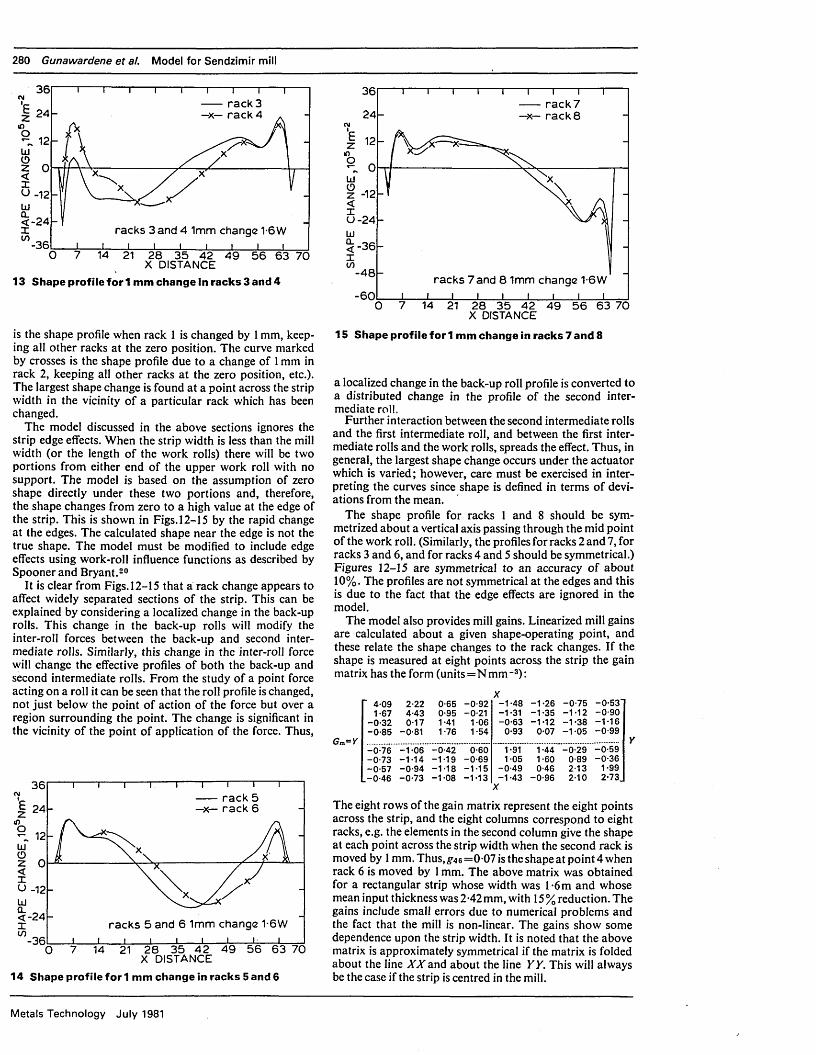
280 Gunawardene et al. Model for Sendzimir mill

36 rack 3—x— rack 424

~ 12

U _12<-24

racks 3 and 4 1mm change 1-6W-36

X DISTANCE13 Shape profile for 1 mm change in racks 3 and 4

is the shape profile when rack 1 is changed by 1 mm, keep­ing all other racks at the zero position. The curve marked by crosses is the shape profile due to a change of 1 mm in rack 2, keeping all other racks at the zero position, etc.). The largest shape change is found at a point across the strip width in the vicinity of a particular rack which has been changed.

The model discussed in the above sections ignores the strip edge effects. When the strip width is less than the mill width (or the length of the work rolls) there will be two portions from either end of the upper work roll with no support. The model is based on the assumption of zero shape directly under these two portions and, therefore, the shape changes from zero to a high value at the edge of the strip. This is shown in Figs. 12-15 by the rapid change at the edges. The calculated shape near the edge is not the true shape. The model must be modified to include edge effects using work-roll influence functions as described by Spooner and Bryant.20

It is clear from Figs. 12-15 that a rack change appears to affect widely separated sections of the strip. This can be explained by considering a localized change in the back-up rolls. This change in the back-up rolls will modify the inter-roll forces between the back-up and second inter­mediate rolls. Similarly, this change in the inter-roll force will change the effective profiles of both the back-up and second intermediate rolls. From the study of a point force acting on a roll it can be seen that the roll profile is changed, not just below the point of action of the force but over a region surrounding the point. The change is significant in the vicinity of the point of application of the force. Thus,

36 rack 5—x— rack 624

O -12<-24 racks 5 and 6 1mm change 1-6W

-36X DISTANCE

14 Shape profile for 1mm change in racks 5 and 6

36 rack 7—x— rack 824

:•— 'X-

z -12

U -24

-36

-48 racks 7 and 8 1mm change 1-6W-60

X DISTANCE15 Shape profile for 1 mm change in racks 7 and 8

a localized change in the back-up roll profile is converted to a distributed change in the profile of the second inter­mediate roll.

Further interaction between the second intermediate rolls and the first intermediate roll, and between the first inter­mediate rolls and the work rolls, spreads the effect. Thus, in general, the largest shape change occurs under the actuator which is varied; however, care must be exercised in inter­preting the curves since shape is defined in terms of devi­ations from the mean.

The shape profile for racks 1 and 8 should be sym­metrized about a vertical axis passing through the mid point of the work roll. (Similarly, the profiles for racks 2 and 7, for racks 3 and 6, and for racks 4 and 5 should be symmetrical.) Figures 12-15 are symmetrical to an accuracy of about 10%. The profiles are not symmetrical at the edges and this is due to the fact that the edge effects are ignored in the model.

The model also provides mill gains. Linearized mill gains are calculated about a given shape-operating point, and these relate the shape changes to the rack changes. If the shape is measured at eight points across the strip the gain matrix has the form (units=N mm _3) :

x4-09 2-22 0-65 -0-92 -1-48 -1-26 -0-75 -0-531-67 4-43 0-95 -0-21 -1-31 -1-35 -1-12 -0-90

-0-32 0-17 1-41 1-06 -0-63 - M 2 -1-38 -1-16-0-85 -0-81 1-76 1-54 0-93 0-07 -1-05 -0-99

-0-76 -1-06 -0-42 0-60 1-91 1-44 -0-29 -0-59-0-73 -1-14 -1-19 -0-69 1-05 1-60 0-89 -0-36-0-57 -0-94 -1-18 -1-15 -0-49 0-46 2-13 1-99-0-46 -0-73 -1 0 8 -1-13 -1-43 -0-96 2-10 2-73x

The eight rows of the gain matrix represent the eight points across the strip, and the eight columns correspond to eight racks, e.g. the elements in the second column give the shape at each point across the strip width when the second rack is moved by 1 mm.Thus,£46 = 0-07is the shapeatpoint4when rack 6 is moved by 1 mm. The above matrix was obtained for a rectangular strip whose width was l-6m and whose mean input thickness was 2-42mm, with 15 % reduction. The gains include small errors due to numerical problems and the fact that the mill is non-linear. The gains show some dependence upon the strip width. It is noted that the above matrix is approximately symmetrical if the matrix is folded about the line XX and about the line YY. This will always be the case if the strip is centred in the mill.

Metals Technology July 1981

Gunawardene et at. Model for Sendzimir mill 281

Conclusions

The derived model is based on theoretical results and the accuracy of the model will depend upon the assumptions made. One such assumption is that the additional stresses at the strip edges due to roll flattening are neglected. This will introduce errors into the final results but the model will be modified to include the edge effects. The results from the improved model will be checked against the present results for accuracy.

When calculating the deflections of the rolls the contri­bution due to shear was neglected. This will also introduce some error which will be checked at a later stage.

The roll-force model does not involve an iterative pro­cedure but uses an approximate explicit solution. However, the iterative solution which employs Hitchcock’s formula is more accurate. These two methods of solution were com­pared and the error of the approximate solution was found to be less than 1 % for typical rolling schedules.

The effect on the final results of variations of the con­stant jS which appears in the stress equation must also be determined. The model seems to produce reasonable re­sults for strip shape, but this must be confirmed by detailed experimental investigation. Normal operating records will be used where possible to test the model, but two coils are also to be rolled for a specific set of shape experiments.

Acknowledgm ents

The authors are grateful for the support of the British Steel Corporation, GEC Electrical Projects Ltd, and the Science Research Council. They are also pleased to acknowledge the contributions to the paper by M. Foster and K. Dutton of BSC, A. Kidd of GEC, and Dr G. F. Raggett of Sheffield City Polytechnic.

References

M . j. g r i m b l e : Chart. Mech. Eng., 1975, 91-93.N . d a v i e s : Iron Steel, Aug. 1972, 391-395. c. a . b r a v i n g t o n , d . c. b a r r y , and c. h . m c c l u r e : ‘Shape con­trol’. 82-88:1976. London. The Metals Society, w. j. e u w a r d s and p . d . s p o o n e r : ‘Automation of tandem mills’, (ed. G . F. Bryant), 176; 1973, London, The Iron and Steel Institute.w . k . j . p e a r s o n : / . Inst. M et., 1964-65,93, 169-178.B. s a b a t in i and K . a . y e o m a n s : J. Iron S teel Inst., 1968, 206, 1207-1213.g . w . d . m . g u n a w a r d e n e and m . j . g r i m b l e : ‘Development o f a static model for a Sendzimir cold rolling m ill’, presented at IM A C S (A IC A ) symp. on simulation o f control systems, Tech- nische Universitat, Vienna, Austria, Sept. 1978. s. u r a y a m a , y . t a k a t o k u , y . n i w a , and Y . s a w a d a : ‘Shape con­trol’, 101-106; 1976, London, The Metals Society. m . d . s t o n e and r . g r a y : Iron Steel Eng., Aug. 1965. m . h e t e n y i : ‘Beams on elastic foundations’ ; 1946, University of Michigan Press.s. t im o s h e n k o and j . n . g o o d i e r : ‘Theory o f elasticity’, 380-433; 1951, New York, M cGraw-Hill.r . s. r o a r k and w. c. y o u n g : ‘Formulas for stress and strain’, 5 ed.; 1975, New York, M cG raw-Hill.g . f . b r y a n t and r . o s b o r n : ‘Automation o f tandem mills’, (ed. G. F. Bryant), 245-278; 1973, London, The Iron and Steel Institute.m . j. g r i m b l e : PhD thesis. University of Birmingham, 1974. g . f . b r y a n t and R. o s b o r n : ‘Automation o f tandem mills’, (ed. G. F. Bryant), 279; 1973, London, The Iron and Steel Institute.E. o r o w a n : Proc. Inst. Mech. Eng., 1943, 150, 140.m . s. g r im b l e , m . a . f u l l e r , and g . f . b r y a n t : Int. J. Numer.M ethods Eng., 1978,12, 643-663.

1 8 . l . r . u n d e r w o o d : ‘The rolling o f metals theory and experiment’, V o l.l, 9-316; 1950, London, Chapman and Hall.

19. s. d . c o n t e : ‘Elementary numerical analysis’ ; 1965, New York, M cG raw-Hill.

20. p. d . s p o o n e r and g . f . b r y a n t : ‘Shape control’, 19-25; 1976, London, The Metals Society.

Appendix 1Roll-bending equations and deflection

An expression is derived below for the roll deflection caused by a point load applied to a roll resting upon an elastic foundation. From simple bending theory the deflec­tion y can be written as

d4yEtg-F-ky .(15)

where Fis applied force and k is the elastic-foundation con­stant.11 This equation is true only if the roll is in complete contact with its foundation, under no load. However, in the case when the roll is resting on an elastic foundation which is bent this is not the case (see Fig. 16).

Let the gap between roll and foundation be Ay under no- load conditions. Then equation (15) becomes:

d4v .EI^=F-k(y-Ay) — F— ky+kAy

butkAy=AF

and

EI^=(F+AF)-ky ................................................. (16)

The solution to equation (16) can be written as

y = ^ j[F (C -D )+ F (F + C ? )J .............................(1 7 )

whereA =sinh2A/—sin2A/B = 2coshAx. cosAx C=sinhA/. cosAa. coshA6 D = sinA/. coshAcr. cosA6 E= coshAx. sinAx+ sinhA*. cosAx F=sinhA/(sinAa. coshA6 — cosAa. sinhAF)F'=F+AFG =sinA/(sinhAa. cosA b—coshAa. sinA6)

1/4A : ' '"(®)!

and constants a, b, and / are defined in Fig. 17. Note also that equation (17) is true only for a concentrated force and when 0s£;c<a. The method of calculating y when a<x^b is to substitute a for b and b for a, and to measure x from the end B.

t y(a)

a n o -lo a d c a s e ; b load ed case

16 Example of loaded roll

(b)

Metals Technology July 1981

7777\

oil resting on elastic foundation

pendix 2

The interference y\z{x) can also be calculated from roll bending using the relation

.mC*)= \{di +dz) — £>12 +yz(x) — yi(x) + J \ v c ( x ) (23)where Diz is the distance between the two centres.

The model proposed by Edward and Spooner4 is used to calculate the work-roll flattening. The proposed model isyvs(x) = [bi+bzp{x)\y-B.(x)........................................... (24)

whereewd I

\2cp{x)\ ..................................

is the Hertzian flattening which occurs between two in­finitely long cylinders having the same diameter and the same elastic properties. Equation (25) is obtained by putting d=di =dz and c = c i = C 2.

Constants bi and bz are estimated to be 0-5 and 0-325 mm t _1 and p in equation (24) is the rolling pressure.

yn(x)=2p{x)c\n • (25)

-fla tten ing equation

is section the local deformations due to flattening in ntact regions between rolls in the cluster and between rolls and strip are determined. The approach follows

of Timoshenko and Goodier11 and, more recently, rds and Spooner.4en two infinitely long elastic cylinders are in contact tal interference yiz(x) can be written as a function of ad per unit length q(x) as

f eW{di+dz) I (*)=9(x)(ci + « )In ...............

e di and dz are the diameters of the cylinder and ci and e two constants depending on the elastic properties, loading is, of course, non-uniform but neglecting d-order errors:

• 08)

)=■yiz(x)

(ci-f C2)ln eW(di+dz) ■ (19)

2q(x)(ci+cz)w variable M is defined to eliminate q{x) from the -hand side of equation (19):q(x)F/w

e w is the length of the roll.

.(20)

)=(C1+C2)

[|n( ^ +rf0 U ,nMk2{FIw){ci+Cz)J

(21)

Appendix 3Elastic-foundation constant K calculation

At various points in the roll cluster two rolls rest on one roll. In order to use the bending equations it is convenient to use a single equivalent value of the foundation constant K. This is illustrated in Fig. 18. This value of K is determined below.

Let the deflection of roll A in the direction df P be yA. The deflection >-ab in the direction Pz can be calculated asj'AB=yACOs(02—6)and, similarly, the deflection ac in direction Pi is given byyAc=yACOs(0i+0).I f Ki and Kz are the foundation constants between the cylinders A and B and A and C, respectively, then Pi=KiyAc

and Pz=KzyAB

butP=Picos(9i+9) +Pzcos(9z— 9) =KiyAC^S2(9i+9)+KzyAC^S2(9z— 9)

but

K=r-yxand we obtain K=Kicos2(9i+9)+Kzcos2(9z-9).

Af«■[:

e2>3(di+dz)2(F/wXa+cz)

)f F/wation (21) becomes:

)< yia(x)(C1+ C 2) lnt e 2/3

+\n{di+dz)-\n[^(22)

2(ci+C2)above equation is true only for positive values of ). Therefore, it is assumed that when yi2(x)sS0,= 0. 18 Equivalent loaded rolls

Is Technology July 1981

Gunawardene et at. Model for Sendzimir mill 283

Appendix 4

Input and output stress profiles

From the geometry of Fig. 19 it can be shown easily thathn*hz+R<f>n2............................................................. (26)

from continuity of mass flowVzhz = Vnftn................................................................. (27)

By substituting hR from equation (26) in (27) we get

Vz • (28)

The per unit slip is defined as

V z — Vns= ■ Vn ■ (29)

From equations (28) and (29) the value of s is found to be R<f> n2s=-

hz(30)

where

, f h z ( h z Hn\� ' J i ^ X r 'T)

id1 ,Jhz 1 —Ul/kl

" 2 2/x | /;i * 1 —crzlkz.(31)

Equation (31) can be derived by considering the roll-gap variables, by differentiating s with respect to cri:

ds _ 2 R . dcfrn

dc7i hz " dai(32)

2R d(f>n dHnhz dHn ' d(f>n

but

d^n 2hz [\ , t J [ f a £fn\l_ = _ ^ +lany _ . T )j........... (33)anddHn 1 1doi 2/i ki—ui ■(34)

19 Roll-gap conditions

By substituting these values in equation (32) and simplifying we obtainds _ a

den k i — a i

where

.(35)

-^[.+,an=(,/f-f)] ............ <36>

• (37)

.(38)

similarly, ds _ ad(J2 kz—oz

but

A s—A oirp— -\-A az-j— =0 .............dt7i da2By substituting for ds/dai and ds/do-2 and simplifying we obtain

2lt7i=y^o2.................................................................. (39)where

ki— aiy — ---------kz— crz

Edwards and Spooner4 derive an equation to calculate the output stress which is given by

A n J x z ft . , Aao A o z = P E T - r - \ + — - hi hz 1 + y

.(40)

Metals Technology July 1981