A Statistical Analysis of Satellite-Observed Trade Wind Cloud Clusters in the Western North Pacific

By Knox T. Williams

Project Leader: William M. Gray

Department of Atmospheric Science Colorado State University

Fort Collins, Colorado

A STATISTICAL ANALYSIS OF SATELLITE-OBSERVED

TRADE WIND CLOUD CLUSTERS IN THE

WESTERN NORTH PACIFIC

by

Knox T. Williams

Preparation of this report

has been supported by

ESSA E - 233 - 68(G)

Department of Atmospheric Science

Colorado State University

Fort Collins, Colorado

June, 1970

Atmospheric Science Paper No. 161

ABSTRACT

Composite upper-air soundings have been constructed relative to 1257 individual satellite-observed mesoscale (3-6° latitude) trade wind cloud clusters in the western tropical North Pacific. Clusters have been stratified into five categories: pre-storm clusters (166 cases treated), developing clusters (211), conservative clusters (537), non-conservative clusters (135), and dying clusters (208). A sixth category has been specified for clear areas (553). Rawinsonde obser­vations from 14 island stations for the two-year period of October 1966 to October 1968 provide composited data for 16 pressure levels from the surface to 30 mb. Approximately 12, 000 observations make up the data sample. Computerized composited summaries for each group of clusters have been made from Northern Hemisphere Data Tabulations (NHDT) tapes for wind, vorticity, divergence, kinetic energy, temperature, moisture, stability, and isobaric heights. Mass and thermal balances are very well satisfied by the composited data.

Significant differences in the low-level horizontal wind shears exist among the six categories. The pre-storm and developing clusters exhibit large low-level cyclonic shears, whereas the remaining cloud categories show weaker cyclonic shears. The clear areas show a marked anticyclonic low-level wind shear. The relative vorticities are mostly determined by shears of the zonal wind. East-west shears of the meridional wind are of secondary importance. These cloud clusters may be viewed as typical of the usual easterly trade wave only if the latter is primarily interpreted as a shearing phenomena of the zonal trade wind.

These observations support the contention of Charney (1958), Charney and Eliassen (1964), and Gray (1968) that low-level frictionally forced convergence (i. e., conditional instability of the second kind, or CISK) in the zonal shearing environment north of the equatorial trough is the mechanism for producing and maintaining these clusters (some of which later develop into typhoons).

TABLE OF CONTENTS

Abstract ••••• • • • • iii

I. INTRODUCTION. 1

A. Background • . . . · . . · . . . . 1

B. Purpose •• · . . . 3

II. TECHNIQUE •• · . . . 4

A. Area of Study and Data Sources . . ... 4

B. Classification of Clusters · . . • • • •• 12

C. Compositing Procedure •• . . . 13

III. DESCRIPTION OF TROPICAL CLOUD CLUSTERS. •• 21

IV.

A. Dynamic Properties • • • • • • • • • • • • • • •• 21

B.

1. Wind Field at Cloud Center • • • • • • • • 21 2. 3. 4. 5. 6. 7. 8. 9.

21 Horizontal Shears and Relative Vorticity. Observed and Interpreted Divergence Profiles 33 Moisture Convergence. • • • • 46 Vertical Velocity. • • • 48 Vertical Wind Shear. • • Kinetic Energy Budget. Absolute Vorticity Budget. Contrast with Clear Areas.

52 53

• • • • •• 59

· . . · . • • • 63

Thermodynamic Properties • • • 63

1. 2. 3. 4.

Temperature and Moisture • • •• 63 Stability " • • • • • • • • • • • • • • •. • Temperature and Thickness Considerations • Comparison of Cluster Categories ••••••

64 66 68

SUMMARY DISCUSSION •• 69

ACknowledgements. 72

Appendix ••• . . . . . 73

References 77

ii

1. INTRODUCTION

Background

In the pre-satellite era, daily observations of the tropical

atmosphere were limited to widely spaced conventional rawinsonde

observations. With the launching of the daily ESSA weather satel­

lites in 1966, a new observational tool became available to meteor­

ologists. In particular, weather satellites have allowed the obser­

vation and documentation of the trade wind mesoscale (typically

3-6 0 latitude) cloud clusters1

(see Figs. 9-12) forming, moving and

dying over the tropical oceans. These clusters have recently

attracted attention because of their hypothesized important role in

the general circulation and as spawners of tropical storms. Sadler

(1962), Fett (1964), and Fritz et al. (1966) were the first to investi-

gate extensively satellite-observed trade wind clusters and discuss

their later development into tropical cyclones. Recent satellite

studies of wave disturbances in the Atlantic trades have been accom-

plished by Frank (1969, 1970), Frank and Johnson (1969), and

Simpson et al. (1968, 1969). Recent satellite studies in the Pacific

trades have been made by Wallace and Chang (1969), Chang et al.

(1970), and Chang (1970). In general these studies have not had

available or have not extensively considered the conventional

1 This name was adopted in the CARP Report (1968).

2

rawinsonde information associated with the satellite cloud pictures.

. 1 In 1969. the later phases of ProJect BOMEX investigated trade

wind cloud clusters. and in the 1970's the GARP Tropical Cloud

Cluster Experiment will be implemented. It is important that we

learn as much as we can about the dynamics of these clusters now.

This study was accomplished with this in mind.

A cloud cluster appears in a satellite photograph as a solid

white mass, an appearance due to the large cirrus canopies typi-

cally associated with them. These cirrus canopies are produced by

outflow from and remnants of the cumulonimbi. In general, develop-

ing and conservative clusters maintain their cumulonimbi from a

steady low-level mass convergence; clusters gradually die when

their low-level mass convergence is eliminated2

Clusters some-

times lose a large part of their cloudiness due to temporary stabil-

izing buoyancy changes from cumulus downdrafts as proposed by

Riehl and Malkus (1958) and documented by Zipser .< 1969).

1Barbados Oceanographic and Meteorological Experiment. During this project, the author participated in several flight missions into cloud clusters.

2The 1969 BOMEX project well documented the 3 to 9 hour or more time lag between the satellite-viewed cirrus canopies of dying clusters and the active cumulonimbus clouds which produced them. Flying under the satellite-observed cirrus, one often ob-. served very few cumulonimbi.

3

Purpose

The purpose of this study is to describe the dynamic and

thermodynamic features of the typical satellite-observed mesoscale

trade wind cloud cluster as revealed by rawinsonde data composited

relative to the cluster center. Clusters have been stratified into

several categories based on their daily life cycles. For contrast,

trade wind clear areas have also been composited. These are repre­

sentative of the clear environment surrounding the clusters.

Most previous tropical cloud cluster investigations have been

accomplished on individual cases or have used only conventional or

only satellite information by itself [for example, Chang (1970) and

Fujita et al. (1969)]. The present study represents a new approach:

the use of both conventional rawinsonde data and satellite data simul­

taneously in a large statistical survey of individual cluster types.

4

II. TECHNIQUE

Area of Study and Data Sources

The western tropical North Pacific Ocean from latitude 0 0

to 30 0 N and longitude 120 0 E to 170 0 W was chosen as the study

area because of the high incidence of clusters (and tropical storms)

and also because here exists the world's best broad-scale tropical

upper-air network. Fig. 1 shows the study area and the 14 island

stations making up the data network.

Composite upper-air soundings have been constructed rela­

tive to 1257 individual satellite-observed trade wind clusters in this

area. Five categories of clusters were established: pre-storm

clusters (166 cases treated), developing clusters (211), conservative

clusters (537), non-conservative or developing-dying clusters (135),

and dying clusters (208). Clear areas (553) make up a sixth cate­

gory. Figs. 2-7 show the positions of all the clusters making up

each category. Rawinsonde data from the 14 stations for the two­

year period of October 1966 to October 1968 provide composited

data for 16 pressure levels from the surface to 30 mb. Approxi­

mately 12. 000 radiosonde observations make up the data sample.

Computerized composited summaries for each group of clusters

have been made from Northern Hemisphere Data Tabulations (NHDT)

tapes for wind, vorticity. divergence, kinetic energy, temperature.

moisture, stability. and isobaric heights. The OOZ data were

0,9",~'C: /-?~'~ -.

• , ., t ,L ~:n!l. ).l! .,\},.. f' . )-i.l .,0 .:-~o __ &9;.-A,<8~~ll1: 0 .•. t .oJ "/:':'y i

"'. 'd , '''1 , , '. j t ""<:. ... ",,'l, ".J?;, . I 0'0 ? o' 'l' t .,. • o· ~~. :;'!. " " '- :,0, " •• '. "~Ji;-~ '. .• .. , ~~.:s,,!.o~'''.':O/-~~~'k + t SH'ltV'~' ,,' '" " /ooS.~~/ . , + t " '10'. ~.' f:l:1 'c-'" "., ,* I "'! '~:/i" ':. '., 1 '.' '" ~

, 0' .•• - -~. ", ~ t t 'II A:W ..

• ': j , • FU -"' , ,p. + I. , , . + • I

' . + f ' T' ~_' __ I_' o - '1'- " S ::- '. ".' , 'I . 1 .., , ., , -- '. ,

' " <. .--. 1 . . I :. ....'.; );". ", IWO" JIM. MAR~US I. t "'.' . .. • .•••• ,; ,

I"'U.A.~I. 4

/

• KOROR

~ ~ ~~~. :. ,',,' /. "": /

-+

.r', 0 ••

Z 0 .,-' .

1 .

:~. ~ .I~.L

~

'SO'

. + ' .,.,. !

.J

J

t>~,' " .. I ,",-, .,1

.~' + ,

+

1.+

, . +

t 'W •• 11"'111' 0 J -~-'" ,I :~ ._ ... '

. ,

1.0·

• JQti.f.S,T.Q-tLJ..-, ~

,,'~~ -f--+--+--. ~+ . I!!Hlwn~M.~.~JL. :

.. :-.: l~tJ~? t. I. -l-.~. + • ~' -r-+-+

.. ""1.-

. + .. :-+/ . - - -t '

-mr .-~~ ... t ' - . 1 L' : ~ :"~, "

s

. ~l .~,o ."'~

~ t ,f'Hqf''',II,J 1'j,IAt.O'>,

< '.

Fig. 1. Upper air stations within the study area.

01

o ~I.-f /?:.' '..::' O.C'Jl , . A"~' I. l·· t i- ' . ~ t '

i~~;o~:-~·,o,~~~,;~I."-T~r-: .1 ' .~ t1-n-l-: 1-1 1-1 +-+-~I---+-'

'X;::(;fr;:';'~~f:H 'T' -·l " 00' • -l '¥

Itoo:

" .~ ~ :. . + . . ~ , ~'. T 1 I

X

o

s w X

•

Summer Cluster (May - Oct.) Winter Cluster (Nov. -Apr.) Centroid of Summer Clusters Centroid of Winter Clusters Centroid of All Clusters Rawinsonde Station

!o~' ,0.

••• - ~- -+--+-~-+---Il0·~t·+---+--f---+--·t-~~)o.~ ! )o'+---+----+----+---+-T ' tit .. 'H t + x ' '. t . . , t, .. .'. A PYA ' "

X K . +

'1. " X • X X

A . IV

~'.-1 . ~~~--+-O-l x +-+---~-~~~+-'-s-T--~~-': MAKU5 l')lAND --, I ,.q

•. -,r. i , /.r l'J ',IAlID')

X

'-:-j I

)Q( X l~ /'"

x '!\'i< x x ";: X t X ~~ ,::~ ~i~: D s

-----------------xf • I" '1'. 1 • 200 -, , ,

'if x "

X

)C 0..)( +)( )( T .~ " • >G< x:- ;..: )( )( X .. WAK ISlAND ,. X ...

X ....

'" )(

'!: • • 4l) ,")( )( x x

• , X

• " .•. '" • j.

{~ :~

;;. ). X X, X· X X X X X- •• , ()()( X ~)(

::+~ ~.~-~~~.~ '" " X " X ,Y -', ° .. X X' . X •

I~' ~ .. X )( ''>~" • lE;')O( S H A {

X

.* • x

'X ;.- * . II 0 • X~· • '. Ox "00 X, .• X

?2; x ~ .( -1 I'V

: ........... ,O.+-l> s I It 0 <D ii' ~,' f·· .4)~ ...... -.,."-+--+- I .. X X 1 )( ~ X X ~

>0 X" O<!lY(. 0 'xOO X Xc!!:>, $'W'J , •.•

? • _ x

'il ~ ~ ><0.

o,;·e l • • ( A ~ C I ~. t • I S A. ~i D S (1)( ___ )(

! . $ .•.•• " .•. ~ ..... +_ ... ~-."-h- ;. ,;, ~ Q; t " 0' -"9~.f,. " T'

. '" . ° .f £)

'Y' + .~

~'" I~../" ?'e:, f~;~~ ~(;) .

--.....:: ~\\I'~>"

v~'~~'V' ,

• 1

:~t ,,'

C-{;p ..,,\: bt ·~t . t

j.

.. . ,t .~~ ~

• "",Ie'. (-;"'.~

!<o I'H=,~~!I !5.A"'~S

Fig. 2. Positions (x's and o's) of all (166) pre-storm clusters in data sample.

;; 1'>',..--"'-

.--~ --~~

c ... / .. s.r...,. . '-"D

S

en

:~.;~}O',~~ ,I 0>

"0"'/;'" t r~ ,y,' , C' ,4",'> i O~ I ,,_~." •• ,. t .;; ':',:;~' .. " . ;';~O'1t ,. ~h I ~'.'-'i i • . ,il l · . ,e,,;:!i. .~ !E1;J~ + ~'+-T'Q'>---+--+-

Summer Cluster (May - Oct.) Winter Cluster (Nov, -Apr.) Centroid of Summer Clusters Centroid of Winter Clusters Centroid of All Clusters Rawinsonde Station

)(

i. /,.,;i'~~' I j • • .. j . • . .. j ,;;;,,~-;,' -.-" I I I" . t )'yr.' ~~'~. I ,~ , • lIt II'~: ' -*--- 1 'r ;

o

S W X

•

''1~1 •

'~.\~

/..;. . ; . j ". I • 'f

, ~ '" '0' 0 -; I' ']0"

'; 1,.' !' r' t 1- .. +

. t • t t t

:1$00

' .• tt.:. A ! . t ' . t . "}' t ..•. w·A · / +. " . . , L ~. . . f . . . . , . .. t . t ' : ~ ~t 1 s t: +~~.'

x

, x'

I '

~'I .. I . t . , ' : VOLCANO ,'5L' i'" , . ., D5 . '" ...• I

';0' MA!FU5 +~o . + t .. )( . t· .' .. ,-1. ~ 1

x

' .... 0· .

0.

Z <"

~----~~I~~~ ~ ~ ~-.-+-+.

x

'" + 160'

T )( t

)(

f )( X !. )(

IL·G

Ie

O WAK'LS"ND

1 " t' X X ;

* x t ~

"fO' . . - I" . . . i,: -i, ~ . .i D, .. . r t-:::~t.~'"' f s nna ,,;2, ~ ... I

)(

I' ""V' 1 ' I ,,..'~

t· .. t· xl v, 1- . t ' t

eO~"";ON .t,.':'o . t Q ' ... r .. r -+-.

)( i

o + t t ' t )(JIE .;. x·· -x x + + t

1'0':. 160' s' H A. {I I-&- ,170' 160' t ~~ ... .. ".

)(... X X + . •. .... X· X S" ,OS . "" ~ X + t " J!C. • . "ia/i" ,.. . . 01'J'S i . ."" )( 0 t "

• .11 --+--t--+--H,'c '" ~o I '11 o·~", II '>'o--+-+--+-+-.'

)( " " lC. )( + •• ~ :- J , X J' Q" + X

• .' ct> + Q., JI< l< X 0 + ;;. t lC!l,., . "0 )( X t X i X X' X 0

/: - +-, ,

800';' *TO.'>0~· .·f >Cl W" OO·~lj.>() t'*iIl' ~""t " c •• 8 L , N , ..J S L • NOS l ' I ,(/ + .' ., ',' .. ~ >V. .; + x .,. x 00 11\ . . . x· "x· T)( I . >¢.'" .

0' ~ ,. X >0.~ . .. x· . ~ .. I·· + til I It' ': '00. r.' I~' ~~ t· "" ••• ~ 0 +".1'0, Q .. , to tIo

/f.~,'· '~O' "to', . . 'T ' . "to' ,.~; " . t' 'r' t' X .'~. :;..S .)!(! " t .. . ," . f . / t . • t .. \r-..!:> I. _._ .s.~ ----1_ _

'W,~ . 1'9 /~ I I . '.' " '~-. '1' . ! . v' . ! ''; ·1"..' 'I' ' .. ' 'I' 'v' '1' .. . ...- . I" . 1 c;; ~_S '. \ t~? . t···· t .... .. ..... .."' ,,~.... ;i,' . 'ta. .... . ... J . t . T . ~. . '~' '-;.--",'" ;"~~ . .. t '~. .,.,..... . ...... ~ "'. . .. , ... .... i t v ~' ~ .'/" +~"1 ,~, ,. '. .. .. . t . . .. ..,. . ~ .. ... PHO'N;~S;A os' . .. . ., t . ""::-.:J. '\ ,\.. . • ! ,~ .. "-.... .. . l. ., ,... ,.,. . .. .... _ .. .. •

Fig. 3. Positions (x's and o's) of all (211) developing clusters in data sample.

i t

-J

1St t

11. T t

- 170' . ~ :I~:

·1: -'j x";,,· : 'jT . +: - ~T' l( :1-.. f~ zt . , .WAKE r5lANO . <!".g. " ,,+. X t" IIX,..·"··

+,.. X "0U ,t'1 +" x X~, ~ * x ~,. l~ x x ~)( r

" "

'1 .. . 'f *.: ~ . 1Jl~: '-"1 '~"-'1' 1 ._. 'l'~ "0;" .. t."'i:=· ..... : ................ . _' .. 0

~> -~'\.~ "=:·t" .~.: ~.

"* " >C).

" " ,,]II( .

/ ~ .

..2

). no' ; ~ j~+hF I II" . ;'1;.. ! ~~ ,.. t 050' X +}. .. . P' " .9.t . 0 x 0 "0' . " . - til ii • +---, ~ I * . . 5" .' ">,,,,'t~.

o to' til .:t .... ~y . rOO ~ '~I[' . . t X" . 'O'_-+7s~hlI---<-+-+-

F~'i-'~~ '17' '.:' . * ~:oo 8":,, II .~. .. . .. ~ >C) " JOe X " , . ',.' .. . " ~ .... ,~ . .;f,.::T : : : : 0 ,.. . 0 ",," ~ IT ·lI.,. . ~ /"1-

.... '"

" Summer Cluster (May - Oct.) o Winter Cluster (Nov, -Apr,) S Centroid of Summer Clusters W Centroid of Winter Clusters X Centroid of All Clusters _ Rawinsonde Station

.JO~NS!O~ l!lAND .

l(

rHqEN~~S:LAJ~s :

r t

.//J ("

. .-'~ T/s ...

. ~os· .1~ _ £ .

Fig. 4. Positions (x's and o's) of all (537) conservative clusters in data sample.

C):)

)( Summer Cluster (May - Oct.) o Winter Cluster (Nov. -Apr.) S Centroid of Summer Clusters W Centroid of Winter Clusters X Centroid of All Clusters • Rawinsonde Station

I

~~~~ .........

. ,,,,.' ~ t "t. ,w t ,,<:+ . + + I( t t T 0 4- .;;.. .j. ",'" 0 + + "

'-40· 't" '50· t 160· S t1 H A I l 119" . ~ + + ., . . , ",;"/:" . ... I .s X

x xO +0. "t· •. S.· ;ll,L"",o

~. .-+-<---+." , ..... c~o r "i I I " 'ox' I' • 1I'~'O"o, I Q) ,II • TO. • . .. + 0 + +. . x ., •.• '. fi';,· ",,"'+

. ~ x X.· . .). x )1£). T' '" + >CJ . + w",$' XQ" oo! 0 .,. 0 + 08.j. ,f 0 + ~ r 0 . • + • 0 ". 00 I( .: t •. x It

:CAROl -iE IS~AN S . ,J<., G ." + 0 I ..... w.. + . ,. t ~ •.. ; .... 0 ! " ... ' .~ 0 0 + )() x

/-.~--~, t Q) , f Q) III .. t Q) II! ... Q) , • .. cf, II .0 II ~ : II. II If ~. c:>. e· 0·)( X .l

".,.,." 0 •. ..'+ Q .•.

~;~ \;. T t T ·4 T' ?: r 's

~:;, /~~~~'.~ .. I • . . . ..+ ; ~ .'.\....:J.'.~. t .. ..... = . +... t ~ ~,,:::::;='\; ..... ~.. .p. t'Q".,\ " . ',;: .£~) ,""")- f\ : I ~ \ '" of

• x x

"

t . r

" I o )( Ol) t-

*

. ,la· . i

~HOfNl~~S~AJD5 .

j.

.·I'.i··~ t •. /"1" . + . .

I~.· !V{)s'

T :;.

Fig. 5. Positions (XIS and o's) of all (208) dying clusters in data sample.

co

;,,~~,~~ 1;~\. .V + .. ~... t + t t .~~~~~;-'M~'" ~+-+-.+-+-+--+-t4o'>---+--l--+ : I "0·...... ~ I 0'0-+-+1 -+--+-I-+-+-+~ x Summer Cluster (May - Oct.)

Winter Cluster (Nov. -Apr.) Centroid of Summer Clusters Centroid of Winter Clusters Centroid of All Clusters Rawinsonde Station

[1,.6 - .;. .' .... .. t . . ~'~, t o

o ?'o::" t·dJ···l······ 'j' ·t ·t' )' :-"',,'%1l:t1A:f: , ! ••. i" •... . I

'·f ,-- ~\ j

• 1",0:

s w X

•

i· "" ~ " 0

"-'~ •• ~-:,' :>

.- •• ; ,+

.<.llC:A"';O ~tAtJD'5 . 0

'-~T 4-

•

"'!. D, Z ' ~ ~. ~t .:.

t •

.;+1,0-,

/ . "

16iJ'

T 1 + t .

t ---+--130· ... ---+---1 ~~~-+-~)O·.....,o--j--+--+-+-+--+~ ..... •

. t t +

t . : t .. t . t

.• -:-+.+.~.,--t-.~+~~.- .. ~I • ~t >-+--+-+-fl~rt-+-i-+-+-I j' I I.~--+-+-+-'-+-·· MAiC~!LA"O . + ... i. .. t . . . . t . )( . . .. II·· ~ ... S 1" . . . t

,x "f"':;:" · •• "to ...• ••• ·.~~~~~D )(. ..• . .• . .. .. .... T . . . . t ,'~ .,;::';f<i'; t S _A." ~ 'f(- ••

X t ' .• I:L d~ :A I t .• I .. Aty

I t "t. )(

WAU rS1At.,lO

, t ~, j.; . °1 .~ f I ['i I ~ .. t ... ' .1

.' • I .. '''"''~ .. '" . , ~, ' , • , . ,:: t

ill. .4-;+ HO&' """" .• '+" A.'.< '1~'.)( 1 * I t .. , ~.~.'_.'~'. .,'.5,", ,,*'j 1'1 • .' ,'. 0,. • ~-iX~ ~ .. ,> • ' ,~ • t j • I ,_, , ..... • , .• .. "', " , I j ...., ~',.. ' ' , • " , , ". ' .. .,' • • "',. , t . .,

.\

-- )( -." ...,......_~_ .. ' ~." . 0 0 + .' , '.A NOS.' + 0 0 Vi ". _.: 0 . ... .: ~O t t~·· I' ~ , ., . . . . . ~ 0 .," t e I . +---,-" " j •• •• • ' . ,'"

',' ," • ' ~ ., . • -; , • .& • 0 0 • • I ! t. . . i

;,' j'"p , ; I ,,' .; J.,. 1 •• , ,. ". ,t' ;. ,,,J"., _, . ~ 'j. t, ,~ • ", t· I ' , ,,2': ~ :=-~:'~'" ' " ," 0 ,'" , , '" ,J,. , 'f, ....

" "" ,/ "1 «e" . . • eo-" - • . ,.... "~.. I . ",,';' 0'\ . t· .' .' t '~.g ~ .. + ~H~EN;~S'LIIJOS .

/.

Fig. 6. Positions (x's and a's) of all (135) developing-dying clusters in data sample.

.... o

'+7' . I ~ .. ' .... T ;:?;h:-,o0)L. ,.... .~~:" t .. . --+---t-~..L+'- ~---+----f40'1----+---+---+- ,., o'~+-+-~>--l--+--«'

;;~:~o, I • J ',,:,l;l f ~~,b€;-~j ~ .. 1. r~'"'¥)

"0)''1 o~, ~': i •••• ~,' .~;,. ,

• ~,; ?l~~-. ,. ':~'''.. t I I I I t't I ::"1'2 /0~.J;;"!!?J;., /'0, :l~ '.~~ , t. ' '. '1':,': ~""/.r{i"J .. 'I + I /t ,~~; ~ ,', '.~ ,.. .. :~. . ; ". t "rTe. . 17

tO' x

~;; .. :~~ )( + )( .. 't + •

'~-~o', ' l : . : f : o.~· t>---+--+-+· '~f .' ft.t+ ..

I' l'

'0' I

x

o

S W x •

" '* t .* f txt .!::L .4 I t, '~" ,. x; ~ )( x f-..)C )(.. 0 • . I W

! -- x x x 'i: ~ : " "" "", t x '" .\I + " XiX X <\%, xx," >Cl( 0," "OX' C>F + 0>0+ '

.~.

Summer Clear Area (May-Oct.) Winter CI.ear Area (Nov. -Apr,) Centroid of Summer Clear Areas

Centroid of Winter Clear Areas Centroid of A II Clear Areas

Rawinsonde Station

t 'i '1

I 0 fB~' . + ~ . x X· . .T. + '" €I €I 1)CO .. X)( .. ..

, ' ~ .. "1" ,. w---..,...- ... --.-----.----JI,..,. "'"' ~ III 11-+" .. -+-- .... · £' ~1' ...... ~ • 0 )( 4> "" '" V I NQ lSI: €I x :)( MARCUS *NO)( )( ... ..• l«) X 0.. €I ;. €I ..

)( Ik • X ''i' X ·6.'}' 0 0 * 0.. I . X )() 0 + 0 . 17 v'

." .... ~-,,,,. , S X 0 • X • Q)() 0 oj) xo x X + )()( C~)( . €I €I X , t .~ ":~"" :

)(i)( ,.,.0 ,- "'. " " U~MOsex :AE~ Q .~ I¥! ~ cJ, . . g I ~, ~

€I "0 ~ X ;$.00 €I )()( . lit ,. 0 0 . >Cl( X t .v', z,. • 11. €I 'W AKE 151AN8 '

:.: 0 >40 X )( _0 00 6~ o QlCJ(OXQc:)(4>Q=>(,)( ~ 0 0." €I,,, 00 - cc t X 0 X >«>?,.. ~. : Q.)( r!' -.. 0 t X *' til X 000,. €I t., . . 0

X

G> '"

o )(0 - K .')CO 0 q, X .... 1\ xO $ $ 0 0 ... . c;) , )( t~O~N5 !ON 1~IAr-.;

,,~~ -<i> '-iO!G-' +-~ -~ ._,&--~ .-~- -= ........ ~-~ ... +-~-J<---"""'~ +----+---+---t--+---o-+--+---t~--+--~_+___t_-+-,-XX OX 711X" XO -€I €I 0 4> >It X t . + .. ;. •

o 0 "0 0 7"" ,. X >40 ,. tII)() ~>«> 0 ,- H 0 A 0, ,00 ,il"c!> 0 T "t, • 0=' . 0 0 .. OX • ~. 0 X . itS' €I 0 + t t

X I JI( X • <:) 0 ___ X + .- .... ~ Ox .~ .f -1 -9 X-+-+

jI.~~-,,--- --, ~-- >4Q-.~:. +--<--<lC~-+-ee>-°t<o,+- ·-e--+t-+-+--+-~+--+ Q •• '" ..r

... lC'-l---- ......... __ ---+--.. ..I

o

/'

)tJ

~\~~ 1+

0"

o x o

o

- 00 0 ~ ••.•.• 0'''', €I

X X >II' e ~ 0.... ·00 X 0 + -. to,;, ,. 0 .l-

• 0 "Q X .b - X ~ II +' II * X + 0 '0 +.. 0 + 0 . ; )I( \. A ". 0 I I .)c~ >- Xl ,> ~ "t ~ ~#' . t·· 0 + 0 .• + ~ '? "//1-,J +-. - .. -. ~--t---'-- .-~ -Ji<-.-__ o-~ .-. n' )(ip. ,.,.. 0 ,.1,,_ * O.f. X >Ox to "'. -; 0 t -t •. /"1:'!t

,fir . ,,;. )( r X· , . . 'i' ><0 . , ,~" 0~, Q;, t . 0 .fo' ,.t· ." s )( . + X . t$ .. + t· 0 .8, 0 t ; .w

. 'b'!. . 1- . . . ~; . fr . ' 's

~ ~~ .;/~~~ ~~~ . t· ~-t = ~l '" '--'--_~ .. ~~ + . <='

~l , ~\.r. --' ---+~ _. ;,;p D i 4~ -to + . - ·110· j I:' (~' c;:- __ . v . ,"I ~ ~ ~',

../ '" . :--:: '\ (.- ~ . . . . . . . . "'-. .. ~

~Hq~NI.X IS.:A _ os

Fig. 7. Positions (XIS and o's) of all (553) clear areas in data sample.

~

~

12

CLASSIFICATION OF DIFFERENT TRADE WIND

MESO-SCALE CLUSTERS - all at some latitude

I I I I I I

101

8 I I -15°N I I Deveiopin~k

Clear I Dling ~ : I Ii

1601

(}JI I -15°N 9 I I ........... I I ••.•..... I I I ill' I 7,' .. I I

10 ~ 101 I Clear I 101 -1!5°N « I I I !onservotive I,.:: I 0

I I I iii

! I 10 I -15°N " I I -:.:-:.:. I I Cleor I I," .. I Del.-Dlln~L

I) / / I' / /1 I Oil CD 12 / / /1' / /1

I I '.':-:-:-: I -15°N 1/ /<;,It;,or/ / (////d I I 7." ..... I

13 I II I I -15°N I I Cleor I

I I I I I

150° 160° 170°

LONGITUDE

Fig. 8. Illustration of cluster classification scheme.

extensively analyzed as this time period was very close to the time

of the daily ESSA satellite photographs. In addition, data 12 and 24

hours before and after this time were also utilized to obtain tendency

changes.

Classification of Clusters

Fig. 8 pictorially shows how the clusters were classified,

and Figs. 9-12 show sequences for developing, conservative, dying

and non-conservative clusters, respectively. Only trade wind clus-

ters have been considered. Developing clusters were ones which

could not be traced backward 4 to 6° longitude in the trade eurrent

the day before their observation but were observed the day after 4

to 6° to the west. Conservative clusters could be traced both back-

ward and forward on the previous and following days, respectively.

13

Dying clusters could be traced backward the day before, but were not

detectable the day after. Non-conservative or developing-dying clus­

ters had a life cycle of less than one day, not being detectable on

either the previous or the following day. Pre-storm clusters were

those that eventually formed tropical storms or typhoons. Clusters

were placed in this category from the day they developed until the first

indication of an organized circulation as seen in the satellite photo­

graph. Clear areas were picked where at least a lOO-latitude-square

area was free of cloud cover. The final category, All Clouds, is

simply the sum of the five classes of clusters. An individual cluster.

will develop, often be conservative for one or more days, and then

dissipate. This cluster would fall into three of the cluster categories.

Because of natural satellite picture uncertainties, some sub­

jectivity was encountered in applying the above classification scheme.

Nonetheless, it was established and found to be a very workable

method for specifying physical differences between the statistical

sumrnaries.

Compositing Procedure

Because of the sub-synoptic size of these clusters, no present

tradE~ wind data network can adequately describe individual cluster

dynamics. However, data for many individual clusters composited

together make a detailed broad-scale analysis possible. Various

dynamic and thermodynamic relationships can then be determined.

March 30 March 29 March 28

Fig. 9. 3-day sequence (March 28-30, 1967) of ESSA satellite pictures showing a developing cluster (circled) on March 29. No cluster is detectable on March 28 in the circled region upwind. On the day after development, the cluster is observed about 8° longitude to the west. A trade wind clear area is evident on March 29 at 150 N, 175 0 E, just north of the developing cluster.

August 7 August 6 August 5

Fig. 10. 3-day sequence (August 5-7, 1967) of ESSA satellite pictures showing a conservative cluster. This cluster (circled) is evident on all three days and is progressing in the trade flow at a rate of 69 longitude per day. Sun glint is visible on August 5 at 14° N, 1749 E in the center of a clear area.

May 19 May 18 May 17

Fig. 11. 3,..day sequence (May 17,..19,1967) of ESSA satellite pictures showing a dying cluster (circled) on May 18. This cluster is easily traced backward the day before, May 17, but is barely detectable on the day after, May 19, in the circled region.

March 19 March 18 March 17

Fig. 12. 3-day sequence (March 17-19, 1967) of ESSA satellite pictures showing a developing-dying cluster (circled) on March 18. No cluster is detectable in the circled regions on either the day before or the day after. Note the clear areas centered at 150 N, 165 0 E on both March 18 and March 19.

:J: I-0:::: o Z

18

COMPOSITING OF DATA RELATIVE

TO MESO-SCALE CLUSTER

WEST

x I I

EAST

X

( X - UPPER AIR SOUNDINGS)

x

Fig. 13. Illustration of compositing scheme and rectangular grid centered on cloud cluster.

Fig. 13 shows the compositing scheme. A rectangular grid

consisting of 4°-latitude squares and extending out 12° latitude was

centered on each satellite-observed cluster. Surrounding each in-

dividual cluster, there existed a pattern of upper-air stations fall-

ing into the various 4 ° -squares. Each cluster within a given cate-

gory had a different array of stations surrounding it. The data from

all observations falling within each square were then averaged to

provide mean conditions around the composited cluster. Fig. 14

shows a sample printout of one of the computerized data composites.

19

!"ARA-tETERS- T(C~ ItHIPC) T~ETAIKI THETA£(K)

•• ~ ••• l?"'.~""~~~'~"""""'.J~""""""'O ••••••••••••• 4 ••••••••••••• 8 •••••••••••• 1~ ••••••• 21.0 • ~7,1 • 21,7 • 2~.2 71.1 21.4 ~1.6

.1L .. _._. __ . __ ~_~ ___ .. __ ~_._-3-0---_____ --2ll -------_ 2.1. -l4 30 h~,1 6~.j 70,0 ~d.R ~Q.O 71.2

12 299.2 2'19.7 299.2 29A.9 299.1

334.1 33".7 3"1·9 333.4 ................................................................ -.. ............................................. ~ ................ --..................................... ", .............. .

1b

8

'Ib

__ It

____ ~.d

??,b l?~ 22.7 72." ,,;.3 22.5 27.5 3:. "c; "0

7;>.6 'I. U b 7.1

3n'I.2 j(;o,'; JOO.2

31"',2 3jQ.'> .135.9

eI, "4 ~j

7?b 71. 7 71.5

300.1 jOn. I 101.n

34'1.1 J4,I,9 j"0.5

• .9" ___ 117

3~1.0 301.2 101.1

34~.7

l5 31 711.1 7<;.7

29':1.9 7'1'1.8

3]b.1 3~1l·7

70 C;7 73.1l "P?,.9

301l.h 31)0.7

34U.h 340.2

R3 • 10 .. 7R.7

34301

70.4

300.0

336.<;

72.4

300.6

339.6

72.6

301.0

341.1

37

65

76

7n.4

1"".0

31 ... 8

71.8

1011.4

33R.9

74.3

10n.9

341.8

8

"

~ .. -...... --~~~-.. ~-- ....................... ~ ........•..... ............•.....•.•.......•...••. ~1.7 '1.1 23,S "J.b ;>~.i 2].7 2].0

44 "b 55 44 <;4 3 .. 27 77.4 7:",1) 77.u 1:'.3 7<',.6 73.5 70;.2

" 4 3'1I .2 JUI.3 301.1 301.1 3no·7 301.2 10".5

... _--- .. _-..&....--. __ . -------_._ ........ -34\.'" 3''7,1 34J.H 34J.l 342·2 342.5 340.9 .•...•...........••.......•...•...............•..•..•.......•......•.•......•.....•....•....••.•••. ~1.. ~).5 23,h 2J.~ ;>].7 23.6 23.7

7.5 L1 ;>t> :11 ;:Oil n 30 7'1.5 1<;.~ 73.0 7:..3 74·3 72.0 (,'1.4

.Ji ____ - ------_ .. ----+-------.--.---~.----.-- - 8 300.<'/ JO\ .0 301.41 3~1.0 301·2 301.1 101.2

J44.5 34].1 141.'1 J42.7 34?8 341.2 34n.l .•..••......•....••.........................•....•..........•...•.•••.•.........•••.•.......•...••• 21.':1 il.7 24.5. 2".2 ?1.4. 23.6 ?l.7

-~._ ... _. _____ • _.2L. - ___ .~._._.~ _____ ._ll ------l4--------~.-- 10 • 71.<'/ 7~.u 63.0 72.2 77.7 76.5 7l.5

12 12 3U 1,-1 102.1 300·9 301.1 101.3

347.3 • J.?~ • 339.3 • 34J.2 341.0 343.8 147.7 • .............. .1.2 ............... -•• A ••• ..... _ ..................... -r.,,- .................... ..Jl.. .. ·"W-O ............... _"'4_ ...... -.-.~r0-9 ....... ~9~~ .... •• 1 i'-... -W" ••••

Fig. 14. Sample computer printout of the composited data at the 950 mb level for the conservative clusters (type 3). For each box, the number of observations ~nd the averaged temperature, relative humidity, 9, and ge are shown. The numbers along the outside border iridicate the degrees of latitude north and south and of longitude east and west of the cluster center. The center is located at 0, O. At this 4" -square center box, there are 115 observations which yield the following average values: T = 23. 10 C, RH = 78.4%. 9 = 300.6° K, ge = 342.9° K.

20

The properties of trade wind cloud clusters presented in this study

are derived from these 4 0 -square averaged composites.

A determination of the representativeness of the composited

data is presented in the Appendix. A discussion of the sample sizes

and standard deviations of several of the parameters treated is also

given in this section.

21

lIT. DESCRIPTION OF TROPICAL CLOUD CLUSTERS

Dynamic Properties

Wind Field at Cloud Center

Figs. 15-17 show profiles of the zonal wind with height for

the pre-storm clusters, conservative clusters, and clear areas, re-

spectively. The profile at the center of the conservative clusters

shows that the typical trade wind cluster is embedded entirely in an

easterly current which extends through the depth of the troposphere.

The zonal wind is strongest in the lower layers, averaging 11 kts.

At 200 mb, the zonal flow is typically easterly but considerably

weaker than the low-level flow. This is primarily due to the varia-

bility of easterly and westerly winds in the upper troposphere above

the lower-level steady trade winds.

Though not shown here, the meridional wind is observed to

be weak, less than 3 kts., at all levels for each category. The hori-

zontal shears of the zonal wind primarily determine the relative

vorticity.

Horizontal Shears and Relative Vorticity1

In the low and middle troposphere, the trade flow is revealed

to be stronger north of the cloud center than to the south (see Figs. 15

1The central 4°-square average vorticity and divergence values were determined from 8° wind shears across the box centers.

.a E

100

150

200

250

300

400

~ 500 IIJ IX :::l III

:!lsoo IX IL

700

800

900

22

,

, , , ,

,

" ,

, . , ,

\

\

\

\

,

" . . '. I , ",

I " , .1 • ••••

950

SFCL----L----~--~~~~~~~~~~~--~

" ., . -30 -25 -20 -15 -10 -5 o +5 +10

u( klsl

Fig. 15. Vertical profiles of the zonal wind north of center, at center, and south of center for pre-storm clusters.

100

150

200

250

300

., ~ 400 I

~ ,

E I

-500 I . IIJ \ , I IX \ : i :::l III \

~ ; :!l600 ,

8°N \ . ,. IX J IL \ 4°N

\ ,', 700 \ . ,

Cenler , , . , , ' 4°S . ' 800 \ ' 80 S ..

\ ' .' -900

950

SFC -20 -15 -10 -5 0 +5 +10·

U (klsl

Fig. 16. Vertical profiles of the zonal wind north of center, at center, and south of center for conservative clusters.

23

100 -'. " " 150 .... \

200 \ I , .

I . 250 .. I

/.. \ '. \ 300 /. ,/' .. " " ". /

" 400 I . I J:j . . I E I ~ 500

I L1J II: , ::> (f) I ~ 600 I

II: I Il. . I

I eON 700 I

I 4°N . I : I Center

800 :, .' 4°5 J

8°S '. 900 I. .. 950

\ . .. " .. SFC

-20 -15 -10 -5 0 +5 +10 +15 +20 +25

u (kts)

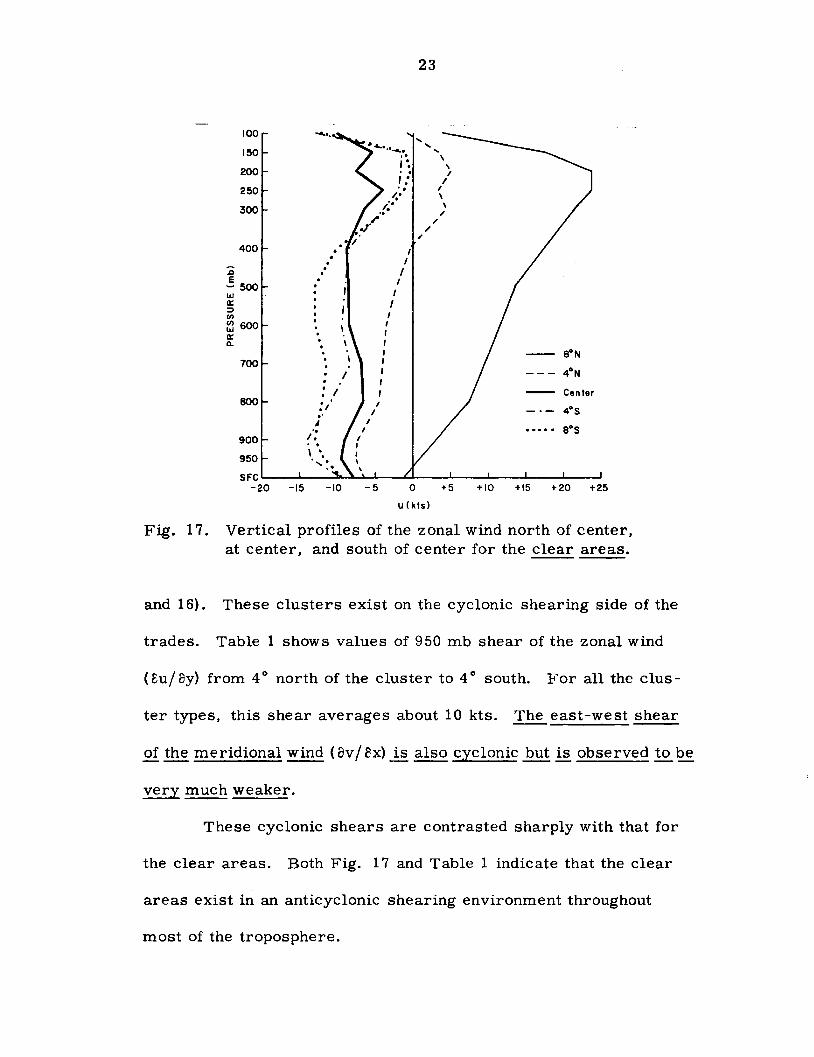
Fig. 17. Vertical profiles of the zonal wind north of center, at center, and south of center for the clear areas.

and 16). These clusters exist on the cyclonic shearing side of the

trades. Table 1 shows values of 950 mb shear of the zonal wind

(Bu/oy) from 4° north of the cluster to 4° south. For all the clus-

ter types, this shear averages about 10 kts. The east-west shear

of the meridional wind (ov/Sx) is also cyclonic but is observed to be

very much weaker.

These cyclonic shears are contrasted sharply with that for

the clear areas. Both Fig. 17 and Table 1 indicate that the clear

areas exist in an anticyclonic shearing environment throughout

most of the troposphere.

24

Table 1. 950 mb north-south horizontal shear of the zonal wind over 8 ° latitude and east-west horizontal shear of the meridional wind over 8° longitude. Units are knots and a positive value denotes cyclonic shear.

Pre- Develop- Conser- Dying Dev. - All Clear Storm ing vative Dying Clouds Areas

-ou/8y 17.0 10.4 9.4 9.6 3.2 10.4 -6. 8 8v/8x 5.3 1.4 2.4 2.4 1.2 2.8 -1. 6

To determine whether clusters are associated with the typi-

cal easterly wave as defined by Riehl (1945, 1954), streamline

analyses at several low tropospheric levels were made. Upwind

from the clusters. the wind direction averages about 110°; downwind.

about 85°. There is indeed 1! very weak amplitude wave in the stream-

line patterns, but there is little contribution ~ this curvature tQ. the

computed values of relative vorticity. As shown in Fig. 18, fully

75% of the relative vorticity at all levels is contributed by shears in

the zonal flow, i. e., -auf &y. These trade wind clusters appear .!2..

be associated, therefore. with ~ weak amplitude wave typified not so

much £l curvature but ~ ~ north-south cyclonic shear. Indeed, in

a case study of a cluster, Simpson et al. (1967) could detect no

noticeable perturbation in the lower-tropospheric wind field.

Many studies of waves in the easterlies can be found in the

literature beginning with Riehl (op. cit.) and Palmer (1952) and more

recently by Yanai (1961, 1963), Elsberry (1966), Frank (op. cit.),

Wallace and Chang (op. cit.). Chang et al. (op. cit.), and others.

100

150

200

250

300

:c 400 E w ~ 500 (/) (/) w g: 600

700

800

900

950

25

au av -t=--+­r ay ax au -- -ay

___ av ax

SFC~~--~~~~~~--~~--~ 10 8 6 4 2 0 - 2 -4 -6

10-6 sec-1

Fig. 18. Contributions to the relative vorticity by the shear of the zonal wind (- &fey) and the shear of the meridional wind (Sv / ax) at the 4 0 -square center box for all cloud clusters. The zonal shear accounts for fully 75% of the relative vor­ticity at all levels.

Some researchers as typified by Sadler (1966) have felt that the im-

portance of the easterly wave has been overemphasized. Depending

on semantics, one may choose to call these clusters waves in the

easterlies or not to call them waves. Should one decide to call them --- -- ---- ----waves in the easterlies. he must realize that they ~ primarily

waves of north-south shear and not of curvature. (The ratio of

zonal to meridional shear is 3 to 1 at nearly all tropospheric levels. )

He must also realize that cloud clusters have typical lifetimes of but

1 to 3 days.

Fig. 19.

26

Cloud Center

200 mb relative vorticity map for conservative clusters. Units are 10-6sec-1•

t 8

..,~

.. % oc -. Uu

Fig. 20.

4

-West Cloud Center

Surface relative vorticity map for conservative clusters. Units are 10-6 sec- 1.

Fig. 21.

Fig. 22.

27

_ .. _-._---------------------_. 100 -10-5

~

150

200

250

300

400

E -500 ~ ::J .. • ~600

800

900

5

~7.5, I " , ,

1 (f)+10 \ ,+ \ \ \

\

\ \ I 1 ,

I

-5

950

SFC~~~~~--~~~~~~~~~--~~ I~ 12°

- North Center South -

Vertical north-south cross section of relative vorticity for conservative clusters. Units are 10-6 sec-1

100

150 -- ... 200 \

\ 250 +2.5 . 300

, I

" '" .-400

:0 +2.5 I \

.5500 I \

~ I \ ,

\ ::J ... , \

~600 , CL

700 , , 800 \ " ,-

\ '" +2.5

900

950 --+2.5- __ SFC

12° 8°

- West

,-, I "

I , 'e±) :+ , ,

\ \ \

\ '+7.5' \

\ 1 I

I I

4° 0°

Cloud Center

, \ \ , 1 1 ,

I I

~:....-____ -5

/' -----7.5 , , " '- --- -7.S

, 0 ,

\ , , " ,

" 2.5 \

8° 12°

East-

Vertical east-west cross section of relative vorticity for conservative clusters. Units are 10-6 sec -1.

o • ~~ ... c o. "U (3

Fig. 23.

s; 'S o (/)

28

,---/' "' I _ )

\ / - -30-......

-20 -__ ---------1 -16

-12

-8

@ Clear Area

Center

-4

200 mb relative vorticity map for clear areas. Units are 10-6 sec- 1• --

12

"E o Z

o ~ .. oCt!! ... c o. IDU o

Fig. 24.

s; 'S o

(/)

8° -West

Clear Area Center

Surface relative vorticity map for clear areas. Units are 10-6 sec- 1•

Fig. 25.

Fig. 26.

100

700

900

950

29

o

-5 SFC~~--~~--~--~~~~ __ ~ __ ~~

12° 4° 0° 4° eO 12° Clear

- North Area Center

Vertical north-south cross section of relative vorticity for clear areas. Units are 10-6 sec-I.

I \

-5

\ I

\ ' '-7.5' -5

700

eoo

900

950 -5 SFc~~ __ ~~~~./~<~'~i~-__ -_-~I~-_2_.5~1~-_-_-~,~-_-

12° 4° 0° 4° eO 12° Clear

- West Area East -Center

Vertical east-west cross section of relative vorticity for clear areas. Units are 10-6 sec-I.

30

100 ;' ;' ,

150 . '" ~ ... .. ... \ 0 ..... ~oooo .... 200 ... .. 0 00

- • 0 . 0

-\ 0

250 0 , , 0

0 , 0

0 , , 0

300 .l . : 0

': 400 , .: - , .: .c ,

E , ~ : E

w 500 ,

0

0::: . I ,

~ . ::::> . . , CJ)

, I , :. . CJ) . , : . lLJ · a= 600 • , : . Pre-storm · , I Il.. - 0

• . . 0 Developing . , I 0

I 0 I , 0 I Conservative I 0

700 I 0 , 0 I Dying 0 0

0 I Dev.-Dying 0 0000 , 0 I 800

, • All Clouds , 0 , 0 ,

Clear 0 , 0 , , 0 , 0 ,

0

900 I 0 I \ 0

\ 0

I 950 \ 0 , 0 ,

, 00

SFC I

+15 +10 +5 0 -5 -10 -15 -20

RELATIVE VORTICITY (l0-6 sec-l)

Fig. 27. Vertical profiles of 4°-square area-average relative vorticity at cluster centers.

31

Surface and 200 mb maps of relative vorticity are presented

1 for the conservative clusters in Figs. 19 and 20 and for the clear

areas in Figs. 23 and 24. Vertical cross sections of relative vor-

ticity taken north-south and east-west through the cluster center are

shown in Figs. 21 and 22. Similar cross sections through the clear

areas are shown in Figs. 25 and 26.

For the clusters. the surface relative vorticity is strongest

at the cloud center with positive values extending more broadly east-

west than north-south. In the upper levels. negative relative vortic-

ities exist everywhere except west of the cloud center. In contrast.

the clear areas exhibit negative vorticity values at the center which

extend through the depth of the troposphere.

Vertical profiles of relative vorticity taken at the center of

each cluster type are presented in Fig. 2'1. For most clusters. the

relative vorticity is positive throughout the lower and middle tropo-

sphere. The pre-storm clusters possess by far the largest vorticity

values; the non-conservative or developing-dying clusters. the

smallest. Note. however. that all clusters exhibit positive relative

vorticity in the lowest 50 mb-the planetary boundary layer. Cyclon-

ic shear and positive relative vorticity in the boundary layer are

1The conservative clusters show nearly identical character­istics with the average of all clusters. The "conservative clusters" and "cloud clusters" are practically the same.

winfer shear = 8 kts.

32

winter zonal wind

summer zonal wind

summer shear = 7 kts.

Cloud \ .. _ _ _ Center

\ \

\

-20 -18 -16 -14 -12 -10 -8 -6 -4 -2 0

u (kts)

Fig. 28. 950 mb zonal wind north of center, at center, and south of center for the summer and winter conservative clus­ters. Note that shears (- au/ ay) are nearly equal for both seasons.

thought to be a crucial feature of cluster dynamics, as will be dis-

cussed later.

Seasonal differences in horizontal shears were also deter-

mined. Clusters were divided into summer (May to October) and

winter (November to April) categories (see Figs. 2-7). Values of

the 950 mb zonal wind north and south of the summer and winter con-

servative clusters are presented in Fig. 28. Although the trade winds

are fully twice as strong in winter than in summer, the north-south

horizontal shears are nearly the same. This is consistent with the

presence of easterly winds on the equator in winter and westerly

winds in summer. Consequently, low-level relative vorticity is

33

nearly the same in winter and summer. The higher incidence and

more conservatism of trade wind cloud clusters in summer than in

winter may be attributable to the larger cumulus buoyancy and much

weaker vertical shears of summer compared with winter. The

weaker vertical shears cause less tropospheric ventilation and allow

for more concentration of cumulus-produced warming.

Observed and Interpreted Divergence Profiles

Surface and 200 mb maps of divergence are presented for the

conservative clusters in Figs. 29 and 30 and for the clear areas in

Figs. 33 and 34. Vertical cross sections of divergence taken north­

south and east-west are shown in Figs. 31 and 32 for the clusters and

in Figs. 35 and 36 for the clear areas.

For the clusters, low-level convergence is concentrated in an

east-west band passing through the cluster center. Above the cluster

center, convergence is maintained up to 400 mb but with strong diver­

gence centered at 200 mb. The clear areas exhibit, on the other hand,

surface divergence and upper-level convergence at the center. Prac­

tically no middle-tropospheric divergence is observed in the clear

areas.

Vertical profiles of divergence at the center of each cluster

type are shown in Fig. 37. For all cluster categories, convergence

is typically maximum at cloud base and gradually decreases with

height. A striking maximum of divergence is centered at 200 mb.

oC

is z

"1:1'-

"'! Oc -<II Uu

Fig. 29.

.s;;; :; 0 en

.s;;; t: o z

"1:1'-"'.! oc u~

34

12°

8°

4"

4°

8"

12°

Cloud Center

200 mb divergence map for conservative clusters. Units are 10-6 ~~c-l •

-1

4° -2

~ ____ --1

o 12"

Cloud Center

Fig. 30. Surfac:6dive::.,ence map for conservative clusters. Units

are 10 sec .

Fig. 31.

Fig. 32.

~

'" .. ..

100

150

200

~600 Q.

700

800

35

- North

I I ,

I /

\ ,

South _

o

+2.5 ...

"

Vertical north-south cross section of diver~ence for conservative clusters. Units are 10-6 sec- •

:a e -500 ~

'" .. .. ~ 600

Q.

700

800

... I /

1- 2.5 ' ....

" I '

I " I \ I 1

I • " 1 ,..... I

" I I I \ I , " '-2.5-'"

2.5- - - .... , ,'-- .............. , / " I I "

" /05 " 900 '- C \.

9~ I

o

SFC~~ __ ~~ __ ~ __ ~~ __ ~ __ ~-~2~.5~~~ 12° 8° 4° 0° 4° 8° 12°

-West Cloud" Center East-

Vertical east-west cross section of divergence for conservative clusters. Units are 10-6 sec- 1

s; 'S o

(/) ,

Fig. 33.

s;

j

0 .... .:tJ! ~c: o· .0 U

s; 'S 0 (/)

j

Fig. 34.

8° -We't

36

Clear Area Center

200 mb divergence map for clear areas. Units are 10-6 sec- 1• --

12°

8°

4°

12°

12° 8° -West Clear Area

Center

Surface divergence map for clear areas. Units are 10-6 sec- 1• --

Fig. 35.

Fig. 36.

37

... ---------------_. __ ._--_._--100 -IQ \ 01

-5 '25

:~-:) :' 300 -15

400

~ .s 500 .. 10 :; .. .. ~600 Il.

700

800 +5

+2.50_~ .,,/ 0 I ,-;,-.......... 0 ...... _,

"I ,\:5 '-2.5'" \

~, C I , \ \ \ \ \ 1 1 1 ,

I I 1 \ \ \ 1 ,

/0 1 , \

o

900

950

, (0 "- .... "- .... ...

\ \

+2.5 I

SFC , +2.5 8° 4° 0° 4· 8° 12°

-North Clear

Sauth-Area Center

Vertical north-south cross section of divergence for clear areas. Units are 10-6 sec- 1

~

100

150

300

400

.s 500 .. :; .. :: 600 cI:

700

800

900

I

","

1 , ,

'-0 \~+2.5 ... ~ ... - .. ~0--_ .... - - - - - -2.5 ... ... '.

... I ""-2.5'

o

Q

, , I

I , ,

1 1 ,

, I

o

950

SFC~~--~~--~~~~--~~~~--~-

-West East -

Vertical east-west cross section of divergence for clear areas. Units are 10-6 sec-I.

.a E

lLJ a:: :::> (J) (J)

lLJ a: Q..

100

150 ,. , ,

200

250

300

400

500

600

700

800

38

0 , ,

, \ \

, ,

, , ,

\ \ \

". "0

\

, 0 • 0 , 0

• 0 ,0 p o o· · · · o • • .0

• 0 o 00 ,

\ \ \ \

900 \ \

950 \ ,

0000-

Pre-storm

Developing

Conservative

Dying

Dev.-Dying

All Clouds

Clear

SFC~--~~--~~~~--~/~~----~--~~--~ -15 -10 -5 0 +5 +10 +15 +20

D I VERGE NC E (10-6 sec- l )

Fig. 37. Vertical profiles of 4°-square area-average divergence at cluster centers.

39

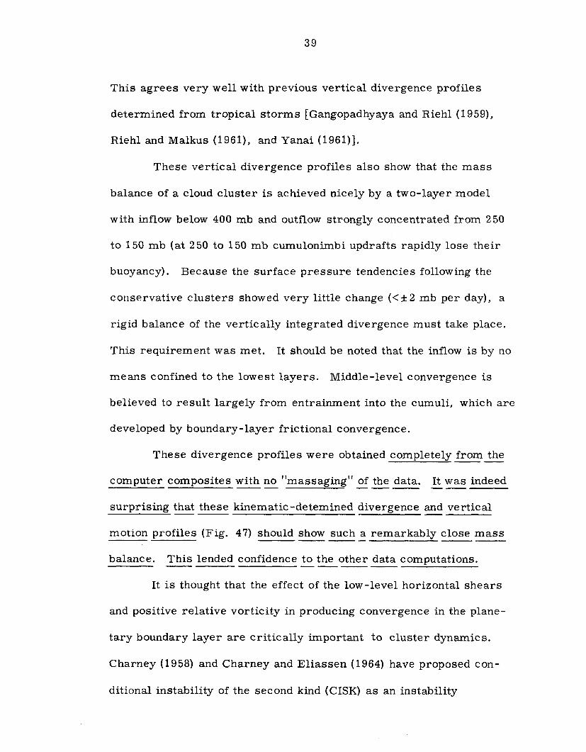
This agrees very well with previous vertical divergence profiles

determined from tropical storms [Gangopadhyaya and Riehl (1959),

Riehl and Malkus (1961), and Yanai (1961)].

These vertical divergence profiles also show that the mass

balance of a cloud cluster is achieved nicely by a two-layer model

with inflow below 400 mb and outflow strongly concentrated from 250

to 150 mb (at 250 to 150 mb cumulonimbi updrafts rapidly lose their

buoyancy). Because the surface pressure tendencies following the

conservative clusters showed very little change « ± 2 mb per day), a

rigid balance of the vertically integrated divergence must take place.

This requirement was met. It should be noted that the inflow is by no

means confined to the lowest layers. Middle-level convergence is

believed to result largely from entrainment into the cumUli, which are

developed by boundary-layer frictional convergence.

These divergence profiles were obtained completely from the

computer composites with no "massaging" of the data. It was indeed

surprising that these kinematic-detemined divergence and vertical

motion profiles (Fig. 47) should show such ~ remarkably close mass

balance. This lended confidence ~ the other data computations.

It is thought that the effect of the low-level horizontal shears

and positive relative vorticity in producing convergence in the plane-

tary boundary layer are critically important to cluster dynamiCS.

Charney (1958) and Charney and Eliassen (1964) have proposed con-

ditional instability of the second kind (CISK) as an instability

40

mechanism by which frictionally-forced convergence in the boundary

layer in cooperation with the heating potential of cumulus convection

combine to initiate development of tropical cyclones. This mechanism

is viewed by the author as a plausible means of producing and main­

taining tropical cloud clusters, some of which may later develop into

tropical storms. Gray (1968) has previously shown a strong positive

relationship between trade wind cyclonic wind shear and disturbances

which intensify into tropical storms. To maintain the cluster, low­

level mass convergence and cumulus convection must be continually

active.

Mendenhall (1967) and Gray (op. cit.) have shown in statistical

studies that significant Ekman or frictionally-induced wind veering

does, in fact, exist in the sub-cloud layer (lowest 600-700m) over the

tropical oceans. Fig. 38 graphically portrays this observed wind

veering with height through the lowest two kilometers for NW Pacific

atoll and ship stations. Average frictional veering of about 10° exists

in the lowest 600-700 m in this trade wind belt.

Due to Ekman-type reasoning, cyclonic wind shears will pro­

duce convergence in the planetary boundary layer and vertical motion

at the top of this layer. The relationship between shear of a zonal

trade current (i. e., positive relative vorticity resulting from north.,..

south horizontal shear) and convergence is illustrated in Fig. 39 for

an idealized steady zonal trade flow with a barotropic boundary layer.

41

200

1500

E -t 10

500

16 12 8 4 0 -4

ci (Degrees)

Fig. 38. Wind angle veering with height in the lowest two km is shown. Wind direction at two km is used as reference. Curve a represents veering of wind with height from surface vessels which were located at .least 10 latitude from any land. Curve b represents the frictional veer­ing of wind with height as observed from atoll data in the NW Pacific; curve c as observed from surface ves­sels located within 10 latitude of land. Note the very small veering of wind with height in the second km layer. [after Gray (1968)]

42

N

W-.J V

SfCI U950mb ,. --

10° ------..--"-- T --Mean Con. _, ~ (Sfc to 950mbf 2 6 Y y = 5° Lot.

vsfC +

Fig. 39. Portrayal of how cyclonic shear in a zonal non-divergent trade wind current at 950 mb can produce sub-cloud con­vergence if a frictional veering of 10° were present. V sfc is the meridional surface wind. [after Gray (1968)]

-- 200 N-

LARGE SUB-CLOUD CONVERGENCE

PRIMARY DISTURBANCE GENERATION AREA

~ DOLDRUMS ~ Eq.T.

1) 4

~IO·N

....... Streamlines at 600m ht.

- - ~ Streamlines at 2 m ht.

~ Vecior Wind Oiff,rence (2m-600m wind)

----- EQUATOR --------()( Frictional Wind Turning

Fig. 40. Idealized portrayal of the difference in wind directions at the surface and at the top of the friction layer relative to a doldrum Equatorial Trough. Note that the wind south of the Equatorial Trough is in general weak and that the sharp cyclonic gradient of trade wind on the poleward side of the Equatorial Trough can lead to substantial low­level convergence by virtue of frictional veering. [after Gray (1968)]

43

The following general specifications would hold for this conditon:

and

_ 1 D.. V sfc 1 C '" - 2" Ay ...... "2 t r (950) (1)

1-w ",,- I; D.. z

t 2 r (2)

where C = mean convergence in boundary layer (surface to 950 mb)

1;r(950) = relative vorticity at 950 mb due to north-south shear

w t = vertical velocity at top of boundary layer

V f = meridional surface wind s c

I; = mean relative vorticity in boundary layer r

z = depth of boundary layer", 600 m

Fig. 40 further portrays the direct relationship between shear and

convergence as it exists in the cyclonic shearing trade current north

of the Equatorial Trough. It is precisely in this region of the tropics

that frictionally-induced boundary-layer mass and moisture conver-

gence occur to produce and maintain the trade wind cluster.

The frictionless form of the vorticity equation on pressure sur-

faces, where the twisting term has been neglected,.can be expressed as

D = - dl;a/I; = -(~ + W . 'VI; + w~)/I; dt a Cit 2 a a p '/' a

(3)

in which D = divergence, t; = absolute vorticity, and the other sym­a

boIs as usually defined. It is significant that this equation is inade-

quate in explaining the observed convergence values especially in the

lowest 100 mb layer. As shown in Table 2. eq. (3) actually predicts

a weak divergence below 900 mb as opposed to the large observed

44

Table 2. 4 0 -square area-averaged ~hvert{1.nce values calculated from eq. (3) and observed. Units are 10 sec. .

layer (mb)

sfc-950 950-900 900-S00 800-700 700-600 600-500

D [ Calculated from eq. (3)]

0.9 0.2

-2.0 -2.5 -O.S -1. 0

D [Observed]

-4.9 -5.S -4.4 -2.6 -2.6 -1. 9

convergence over the 4 0 - square central box for the conservative

clusters. Above 900 mb where gust-scale turbulent friction is insig-

nificant, eq. (3) is more applicable but still falls short of describing

the observed divergences by approximately 50 %.

These cloud clusters must not be thought of as wholly propa-

gating centers of relative vorticity which can be generally handled

with frictionless dynamics. The boundary layer and cumulus mixing

are fundamental ingredients.

Above the planetary boundary layer where gust-scale friction

is small, the horizontal wind shears do not directly contribute to

convergence even though convergence is observed up to 400 mb (see

Fig. 37). The larger part of the convergence above the boundary

layer results from buoyancy-induced entrainment into the cumuli, as

portrayed in Fig. 41. The present lagrangian cumulus cloud models

[Weinstein and Davis (196S) and Simpson and Wiggert (1969)]

45

w= Mz= 5 units

500 mb - - - - t ---1----Required entrainment

= 4 units .-~-

950 mb - -'--~I=-----=t=--...1

... .. M=lunit

SFC 7777777777777777777

Fig. 41. Illustration of vertical mass fluxes (Mz) and resulting required lower and middle-level entrainment into the sides of the individual cumulonimbus.

prescribe such an entrainment. Cumulonimbus typically transport

3 to 7 times more mass upward through the 400 to 500 mb surface

than is supplied at the top of the boundary layer. Significant en-

trainment of environmental air into the sides of the cumulonimbus

updrafts must continually be occurring. This entrainment requires

a large convergence above the boundary layer. Without surface

convergence to form the cumuli~ a large fraction of the middle-

level convergence would not occur. The cloud cluster divergence

profiles of Fig. 37 would then be analogous but opposite to the

.c E

300

500

~ 600

46

.01 P-E ~ 2 cm/day

.04 (2%)

.11(5%)

~ ~~~ .IB( 9%)

~ 700

BOO

900

950

SFC 0.0

.56(27%)

.89 (43%)

0.1 0.2 0.3 0.4 0.5 0.6 Water Vapor Convergence (Cmw/doy)

Fig. 42. 49 -square area-average moisture convergence at center of conservative clusters. Contributions of 100-mb layers are given in cm/ day and in % of total.

clear area profile of upper-level convergence and surface outflow.

No significant middle-level convergence is occurring in the clear

areas.

Cumulus development is primarily a product of convergence

in the planetary boundary layer, i. e., below 600-700 m. In the

tropics, cloud bases typically exist at 600-700 m~ or 950-940 mb.

Moisture Convergence

A computation of moisture convergence for the conserva-

tive clusters (shown in Fig. 42) reveals that although this

47

convergence is a maximum in the lowest 100 mb layer, it is not

confined to this layer. More than half the net moisture conver-

gence into the cluster-centered 4"-square box occurs above

900 mb. Much of the above-the-boundary-layer moisture conver-

gence is likewise induced by the cumulus entrainment-induced mass

convergence.

A computation of P-E was made from the equation

where

P-E =

P = precipitation

E = evaporation at the ground

A = area of 4"-square box

g = acceleration of gravity

q = specific humidity

I. = increment of boundary length

V n = wind component normal to boundary

~p = thickness of individual layers

a at = change over 24 hours

The first term on the right represents the change in water vapor

storage over 24 hours within the volume, and the second term is

the advection of vapor into or out of the volume. The result is

(4)

P-E = 2.0 cm/day, with the advection term contributing more than

90%. If E is assumed to be 0.5 cm/day, then the resulting 4°-square

48

area-averaged precipitation from a typical cloud cluster is 2.5

cm/ day or 1 in/ day. Rainfall of this magnitude requires the

presence of cumulonimbi, and indeed the bulk of the rainfall in this

area comes from cumulonimbi which are maintained by synoptic-

scale cyclonic wind shears.

Vertical Velocity

Vertical cross sections of kinematically-computed vertical

velocities taken north-south and east-west are presented in Figs.

43 and 44 for the conservative clusters and in Figs. 45 and 46 for

the clear areas. For the clusters, upward motion is a maximum

at the cluster center and is confined to a narrow north-south extent.

The clear areas exhibit a broad area of subsidence with maximum

values north of the center.

Fig. 47 presents vertical velocity profiles at the 4!1-square

center of each cluster type. All cluster categories show maximum

vertical motion at 400 to 300 mb. A typical area-averaged verti-

cal velocity at this level is 170 mb/day or 3 cm/sec. The upward

motion becomes zero between 200 and 100 mb. It was unexpected

that the kinematic vertical motion determination would give such ---- ---consistent results. This is felt to be the result of the large statis-

tical averaging process which smoothed out random errors.

49

'--"-"---"--' 100 0 0 +50 150

I

0 I , 200 I

,/

250 ,/

l I

300 I I

I , I \

400

l f f ,

:g , ____ +50

E ~500 a: I

0 :J I en :!l600

+200 I \ I

a: ~15d Q.

-100 +100

900 0 0 0

950

SFC 12° SO 4° 0° 4° SO 12°

_ North Cloud South_ Center

Fig. 43. Vertical north-south cross section of vertical velocity for conservative clusters. Units are mb/ day.

100 I( \' \ I

150 o I

\, -IO~ ,-

I , 200 I -50 , , , ,

-100 -150 , " ,

I \ \

...

f , ,

:g \ I

E \ I \ I

""' 500 I II: :J

,/ VI VI

, ~ 600 , , , , Q. -100 ' ~

700 -;50 ,

I I

,- I

SOO I , ,

/ \ '" -50- - __ .... " --, ,-

900 \ , , --'

950

SFC 12° SO 4° 0° 4° SO 12°'

- West Cloud

East -Center

Fig. 44. Vertical east-west cross section of vertical velocity for conservative clusters. Units are mb/day.

Fig. 45.

Fig. 46.

:;; E

100

150

200

250

300

400

;::; 500 a: ::;) II)

~ 600 a: Q.

700

800

900

50

0

1) +400

:\ I ,,-, I 0 I \ I

I

, \ I

~50

I I

I

I

I

I I

,

I I

I

0 0

950 0

SFC~~--~--~----~--~--~--~--12 8 4 0 4 8 12

Clear _ North Area South _

Center

Vertical north-south cross section of vertical velocity for clear areas. Units are mb/day.

100

)\ It",.",. ",.",

'0 0\\ 150

, , , 200 ',,50'

, '+100 , I

\ 250 , I

I I

300 I +100 I

I ,/

I -- ... , .. I

I ... I \ , 400 I ,/ I \

I 't' \

I I I , +50

:;; +50 , I I ... '-

E '" , I I

~500

1 I , \ I a: ~50 :::J

II)

~ 600 a: 0 Q.

700 I , I

\ I

\ ,

800 I

" ... .... - - +50-

900 0 950

SFC~~--~~--~---J~--~---J~--~--12° 8° 4· 0° 4° 8° 12·

-West Clear Area

Center East-

Vertical east-west cross section of vertical velocity for clear areas. Units are mb/ day.

51

100 , '" 0

'" 0

'" 0

0

150 -'" 0 0°

00 00

200 00

0000 00

00 00

250 00 00 ,

00 00 ,

300 0 0 ,

0 0 . 00 \ . . 0° \ • 0 . 0 0 \ . 0 \ • 0

0

400 · \ · 0

· 0 , · 0 · 0

, ..0

. 0 , 0

E 0 • 500 0 • 0

lJJ 0 I 0 a:: 0 I

:::> 0 0 I

(f) 0 I (f) 0

600 0

w 0 , a:: 0 ,

0 a.. 0 , 0 0 , 0

700 0 , 0 0

, 0 , 0 0 , 0 , 0

800 Conservative 0

, 0 , 0

Dying 0 I 0 , 0 0

Dev.-Dying 900 0000 0

0 0

All Clouds 0 0

950 0

SFC -250 -200 -150 -100 -50 0 +50 +100 +150

RISING SINKING w (mb/day)

Fig. 47. Profiles of 4°-square area-average vertical velocity at cluster centers.

.r; -:::J 0

rJ)

\_ .... _~_ 0

'" -~- ·0"· ......... - ~

-. ,,0..0 _ ........

52

---·-Pre ::'-5 form Developing

Conservative

Dying 000000 - -...,.....

000

"'-4° 0000 Dev.-Dying

All Clouds

Clear

4°

8° -30 -25 -20 -15 -10 -5 0 5 10 15 20

Westerly Easterly

950 to 200mb SHEAR IN U (Knots)

Fig. 48. Vertical shear of zonal wind (u950 - u200) at 4° latitude intervals across cluster centers. Westerly shear de­notes stronger west winds (or weaker east winds) aloft than near surface.

Vertical Wind Shear

Fig. 48 gives the 950 to 200 mb shear in the u component.

At the center of the conservative clusters this shear is westerly

and only 4 kts. The small magnitude of this shear is thought to be

important for cluster dynamics. A small vertical shear means a

weak non-divergent ventilation influence [Gray (1968)]. Any sensi-

ble heat realized eithe r from condensation or from subsidence is

not advected away from the cluster area but rather is allowed to

accumulate. This is felt to be an important process in maintaining

the conservative clusters and for tropical storm development.

Shears at the centers of all the trade wind cluster types

are very small (within ± 8 kts.) by mid-latitude standards. It is

53

curious that the pre-storm clusters are the only cluster type with

an easterly vertical shear at their center~ i. e. ~ stronger easter-

lies aloft than near the surface (see also Fig. 15).

Kinetic Energy Budget

The kinetic energy equation can be expressed as

r saKE JP A at

o A op g

;;; _ r r v KE 0 1. ~ _ r r 8~KE JpJ1. n g JpJA 8p

where KE

8 at

A

p

g

z

k " t" IV2 ;;; me lC energy ;;; z

;;; change over 24 hours

;;; area

;;; pressure

;;; acceleration of gravity

;;; increment of boundary length

;;; wind component normal to boundary

;;; vertical velocity

;;; horizontal wind vector

;;; height of isobaric surface

o A op g

(5)

The four terms on the right of eq. (5) represent~ respectively~ the

horizontal advection~ the vertical transport~ the generation~ and

the dissipation (which cannot be calculated) of kinetic energy per

unit volume. Eq. (5) can be written symbolically as

aKE at

54

awKE (observed) = - V KE - -a-

'-- n p v

- V ~z + Residual (6) n J

aKE (calculated) at

The residual term can be viewed as a measure of the difference

between the observed and the frictionless calculated kinetic energy

tendency. The residual is a combination of frictional dissipation

to heat and any other influences such as cumulus-scale mixing and

possibly some data unrepresentativeness. The residual could not

be directly assessed.

The terms of eq. (6) were computed at individual levels over

the central 4°-square and are presented graphically in Fig. 49 for

the conservative clusters (very representative of all cluster aver-

ages) and in Fig. 50 for the clear areas. For the clusters, the

observed KE generation is found to be small at all levels, with a

very slight positive generation (wind blowing down the height gradi-

ent) in the low levels and negative generation (wind blowing up the

height gradient) in the upper levels. This result is due to the very

small isobaric height gradients inside and outside of the clusters.

The horizontal advection term shows a significant inflow of KE

from the surface to 400 mb and a very large outflow centered at

200 mb. The vertical transport term opposes and closely balances

this horizontal advection. The vertical transport term is seen to

55

decrease the KE of the low levels by transporting it upward where

it makes a large positive contribution centered also at 200 mb.

Neglecting the residual term, the calculated a~E shows an in­

crease of KE in the low levels. very little change in the middle

levels, and a significant decrease in the outflow region of the upper

troposphere. The observed changes of KE over 24 hours, on the

other hand, show near zero values everywhere except in the out­

flow region, where KE is decreasing.

The residual term represents the difference between the

calculated and observed KE Changes. In the low levels, the resi­

dual is negative, whereas in the upper-level outflow region, it is

positive. This residual is largely attributed to the vertical KE

transport by cumulus up- and downdrafts which is not properly

represented in the 4°-square composites. Both up and down

motions are occurring. The net vertical transports are thus

larger than those indicated by the mean vertical motion itself.

Gray (1967) has previously discussed this type of cumulus-induced

sub-grid-scale residual influence.

The conclusion drawn from this kinetic energy budget is

that the cloud clusters, in the net, are typically vertical trans­

porters of KE with little internal generation or dissipation. KE

is imported in the lower half of the troposphere, transported

upward within the cumulonimbus clouds, and exported in the

56

100 .-.-.-.-

150 _._0 -.-0::·-'

200 ..... -.. -.-. 250 -'- '-.

300

400

:c E ~ 500 a: ::l (J) - aKE (Calculated) at (J)

~ 600 aKE (Observed) at Q.

700 Residual

800

\ -VnKE \

\

\ a""KE \ -ap-

" 900

950

\ .~ 0000 -Vnl:t.Z ,

1000 SFC

-20 -16 -12 -8 -4 0 4 8 12 16 20

cm2sec-3

Fig. 49. Kinetic energy budget for conservative clusters: Verti­cal profiles of the terms of the kinetic energy equation. The computation was made over the 4°-square center box, and all values are per unit mass.

57

100 •••• 0

150 • • • • \ ••• 0 , , ,-- " 200 ,1'-- " "

" 250 , /

" 300 0 ,. • 0 " .... 0 ,. ',. 0 " ......

" 400 • 0 ........

• 0 '.0

• ~ • e ~

- 500 o· o. 1.1.1 o· It: o· ;:) o. en en o. 1.1.1600 0

It: ., aKE

Go - at (calculated)

--- ~~E (observed) 700

••••• Residual

800 -VnKE

I awKE I -ap-

900 I 00000 -Vn6Z I

950

1000 SFC

-9 -8 -7 -6 -5 -4 -3 -2 -I 0 2 3 4 5 6 7 8 9 10 cm i .. c-3

Fig. 50. Kinetic energy budget for clear areas: Vertical profiles of the terms of the kinetic energy equation. The compu­tation was made over the 4° -square center box, and all values are per unit mass.

58

upper troposphere outflow to the surroundings. The net effect

is an almost neutral observed kinetic energy tendency.

The terms of the kinetic energy equation for the clear

areas (Fig. 50) show basic differences from those for the

clusters. There is a positive generation of KE in the low levels

but a negative generation (wind blowing up the height gradient -

convergence into an anticyclone) in the high levels. The only

positive contribution in the upper levels comes from the advection

term, a result of the substantial inflow in the high troposphere.

Low-level outflow advects KE out of the clear areas. The vertical

transport term acts to remove KE from the upper levels and to

carry it downward such that there is a positive contribution in the

low levels. The advection and vertical transport terms are thus

seen to act just oppositely in the clear and cluster areas. The

eKE observed and calculated -at curves are similar in the lower

half of the troposphere. No cumulus and no residual effect is

thus present in this layer. A significant residual exists only in

the upper troposphere.

The processes transporting kinetic energy act oppositely

in clear areas than in cloud clusters. The advection and vertical

transport terms dominate the kinetic energy budgets of both envir-

onments, but with much larger magnitudes in the cloud clusters.

59

Absolute Vorticity Budget

The vorticity equation on pressure surfaces can be written as

where

r r aSa oA op = _ r S V S o/. op _ r r aWsa oA op JpJA at g JP /. nag JpJA ap g

- r 5' D S oA op - T + F Jp A a g

Sa = absolute vorticity

a = change over 24 hours at

p = pressure

g = acceleration of gravity

/. = increment of boundary length

V = wind component normal to boundary n

W = vertical velocity

D = divergence

T = twisting term

F = friction term

This equation has also been evaluated for the central 4°-square of

(7)

the conservative clusters and for the clear areas. The first three

terms on the right are~ respectively~ the advection term~ the verti-

cal transport term~ and the divergence term. Eq. (7) can be

simplified and written symbolically as

asa (observed) = - V S - aw sa - D Sa + Residual at '- n a ap ./

"Y a sa

(calculated)

(8)

at

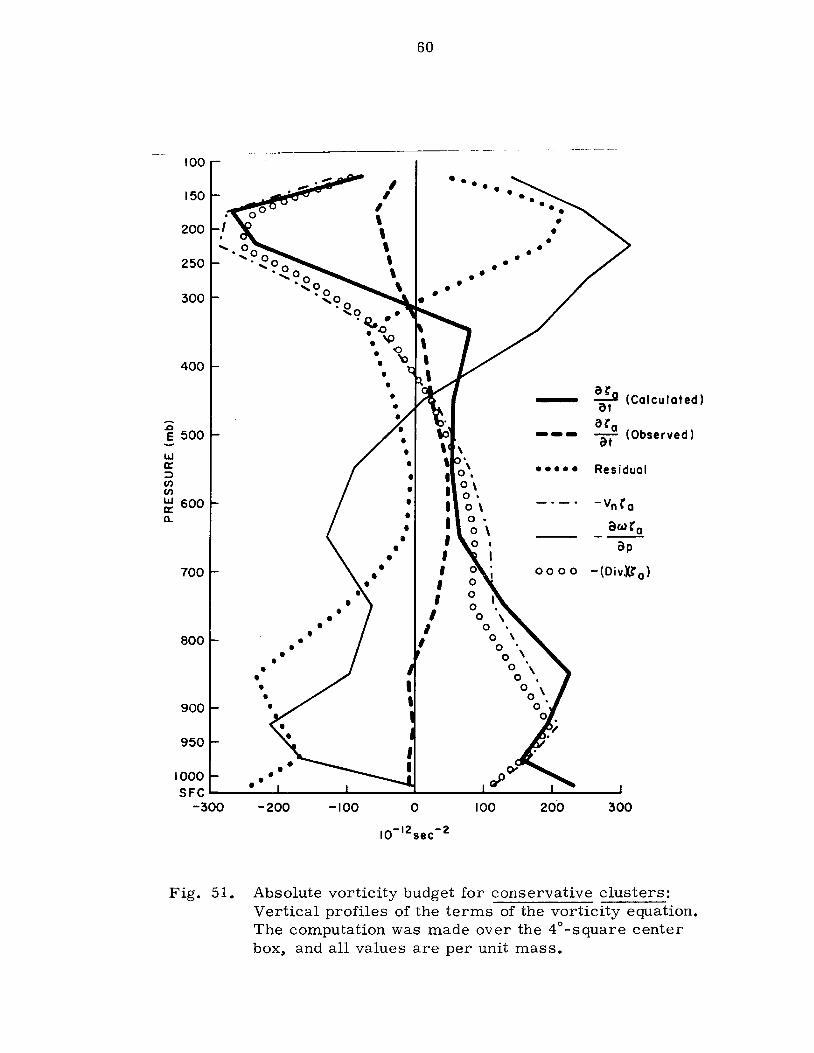
100

150

200

250

300

400

.J:l E 500

LLI a:: :::::l (/) (/)

LLI 600 a:: a..

700

800

900

950

I

• • • •

• • • • •

• • •

I , I

I

, , , , \

60

• •

• •

• • •

• • • • • • • ••

---•••••

8l.' =if (Calculated)

a(a at (Observed)

Residual

-VnC a

_ awra op

0000 -(Div.n"a)

o o o

o o \ o . o \ o \ o . o \

o . o o

1000 •• SFC~----~------~------~----~------~----~

-300 -200 -100 o 100 200 300

Fig. 51. Absolute vorticity budget for conservative clusters: Vertical profiles of the terms of the vorticity equation. The computation was made over the 4 0 -square center boxJ and all values are per unit mass.

~ e

LLI a::: => (f) (J) LLI a::: 0..

100

150

200

250

300

400

500

600

700

800

900

950

61

o o

000

o o

o , 0 ., 0

, 0 , 0

, 0 '0 o

01 0,

o o • •

• • • • • • • , ---., ...

0000

iH' Tt- (Calculated)

eH'a at (Observed)

Residua I

-Vnra

aW~a -ap--(Div.XC a)

1000 SFCL---L-~~~--~--~--~--~--~--~--~--~~

-120 -100 -80 -60 -40 -20 0 20 40 60 80 100 120

Fig. 52. Absolute vorticity budget for clear areas: Vertical profiles of the terms of the vorticity equation. The computation was made over the 4"-square center box, and all values are per unit mass.

62

Here# the residual includes the twisting term and the friction or

sub-synoptic-influence term. The terms of eq. (8) are presented

graphically in Fig. 51 for the conservative clusters and in Fig. 52

for the clear areas.

For the clusters# the advection and divergence terms act

similarly to increase vorticity in the lower half of the troposphere

and to decrease vorticity in the upper half. The vertical transport

takes vorticity out of the lower layers and into the upper layers.

The sum of these three terms yields calculated ~~a values which

are positive below 300 mb and negative above this level. The

observed change is very much less# however # so that a large nega­

tive residual must exist in the low levels and a large positive resi­

dual in the high levels. Similar to the KE residual# the vorticity

residual might also be largely explained by cumulus up- and down­

drafts vertically rearranging the momentum. The characteristic

difference of vertical wind shears north and south of the clusters

(see Fig. 48) and the presence of cumulus clouds prescribe such a

relationship. This influence of the cumulus# of course, could not

be measured. Finally# an integration of the observed a~: values

over all layers for the clusters reveals only a slight increase in

vorticity over 24 hours.

Compared with the clusters. the clear areas (Fig. 52) are

revealed to be much weaker systems. with all terms having smaller

magnitudes. The divergence. advection. and vertical transport

63

terms act to import vorticity in the upper levels, carry it downward,

and export it near the surface. The integrated observed vorticity

change over 24 hours shows a small net decrease. The residual influ­

ence is observed to be much less with the clear areas than with the

clusters.

Contrast with Clear Areas

Although both cloud clusters and clear areas are deeply em­

bedded in the trade current (see Figs. 16 and 17), vital dynamic differ­

ences exist between the two environments. The data for the clear

areas show a striking departure from any of the cloud areas. In the

clear areas, low-level shears are markedly anticyclonic, and relative

vorticities are negative throughout the troposphere. The divergence

profile reveals low-level divergence, upper-level convergence, and a

deep middle layer of non-divergence. Subsidence throughout most of

the troposphere suppresses cumulus development. Horizontal and ver­

tical transports of kinetic energy and absolute vorticity are also weak.

Thermodynamic Properties

Temperature and Moisture

Soundings for the conservative clusters and for the clear areas

are presented in Fig. 53. The clear area sounding is representative

of the clear environment between well-defined cloud clusters. Where­

as there is little difference in the dry-bulb temperature curves (both

have lapse rates slightly steeper than moist adiabatic). it is

64

immediately noticeable that there are large moisture differences be-

tween the two environments. For constrast. the level at which the

relative humidity has fallen off to 500/0 is at 450 mb for the clusters

and 840 mb for the clear areas.

This moisture difference is also evident in the vertical pro-

files of e shown in Fig. 54. e

1 Since e '" - (gz + C T + Lq), and since

e c p p

only small temperature and isobaric height differences exist between

the two envirorunents. the large difference in e is attributable only to e

the difference in water vapor. The drier clear environment is un-

doubtedly a product of broad-scale subsidence, as shown in the vertical

motion cross sections of Figs. 45 and 46.

Stability

The e profiles indicate that the clear areas possess a much e

larger Cumulus Potential Buoyancy, defined as e (sfc) - e (minimwn). e e

than do the cloud areas. Thus, if a parcel could be raised to the level

of free convection, the unentrained parcel would have more buoyancy

and would accelerate upward more rapidly in the clear than in the

cloud environment. However, the absence of boundary-layer conver-

gence eliminates the initial lifting mechanism to allow the parcel to

attain buoyancy. A dynamic constraint exists, therefore, to cwnulus

development in clear areas. In addition, a strong thermodynamic con-

straint also exists. This is dry-air entrainment (see Fig. 53),

65

o ,'1-

TEPHIGRAM FOR TROPICAL SOUNDINGS

@- :#,'

",:=of: *: ' ~ ,r; '" '£.'J' r:" .'Ii

&S '7" >ii .. ,~ '" , ,v .: t.r

fr

./ ".

, i Slation.

Ele'lollo" ____ ..

j r,me_ .. __ . \ Plotted by _ ,

~" " '/,.0'.

',~ o ':::.:' :'i I"t' • ,--n

;_rp:~.::.:.".~:::..:-::, . .r'J:.[.+:' ;··-".::;i:.~914·.~4i.:/'.r~~#., '~*~. ~~l~·~~: ~1;..r:II!mffirll;~·I~;I'I~~ ~ i." .: ,,:'0

'" -., :: " ij ,r,' ' 'r ',14:,~_ " o ' .. " ~.:~,/, r- ,,:;:~, ,:: ',1/v"" ~ :~": :Vi ' ~A,;;~.b,l~r.j'J!.w.!'H'~.:M'f.}h':{'i,u.

f'liil!: p. ';:le

, PC :

~ :'-,

;'1~'

,,:.'

:~ C

.J

QO'1L~"'~":~: ~:t/~'#.'YH"f8;!l:~·~;~··~~~~~~rf;~:' .!:~fru~'B~~: ~~~~~~~~~~m : .' ~~~~ ,,': .; , , t.cz

::jt~;·t~/~:;]~Ij~~:·:.1i~~:~i~~~:~g;li'ji:r:iw~;;;~;;ili' ;i"ill~· ::tf :d;i, '. N. : "Ii; : :' ~

-~~ ':j 11:- i:-~n :-,19 liT, I i-:I

.-:?,C?II Ii -!9,i! '1:191111 I I II I TI iPi '«0 , I ' '.' 'I" , 'I "'" , ,',I" .' I I I , " "f'r.

"30 -120 -110 -100 -90 -80 -"0 -60 -50 -40 -30 -20 -10 T 0 10 20 30 40 50 60 70 80 90 100

Fig. 53. Mean soundings (T and Td) at centers of cloud clusters (solid) and clear areas (dashed).

.<> E

100

150

200

250

300

400

.~ ........ "'­.. ;~ ...... .,. .. ' ,:

,: , : I : , : , .. , :

I : I :

I :

;:;500 I : , : , :

0:: J U)

, . ~ 600

I ! , : , 0:: Q.

700

800

, , , I I I I \

\ \ \

900 ,

Conservative Clusters

Cleor Areos

, . 950 ' ....... .

SFC~--~---L .. - .. -·~~·~· __ _L __ ~ __ ~ 320 330 340 350 360 370 380

ge COA)

Fig. 54. Vertical profiles of ge at centers of cloud clusters (dotted) and clear areas (dashed).

66

causing rapid erosion of cumulus towers. In the cluster areas, on

the other hand, the entrainment constraint is much less.

Stability in the cluster regions is also affected by cumulus

downdrafts. Zipser (1969) has observed that these spreading down­

drafts strongly suppress cumulus buoyancy for a few hours. This

may offer a partial explanation to the frequently observed pulsating

nature of these cloud clusters.

Temperature and Thickness Considerations

Fig. 55 compares the heights of isobaric surfaces in the cloud

environment with the heights of the same surfaces in the clear envi­

ronment. The isobaric heights in the low levels of cloud clusters are

lower than the same isobaric heights in the clear areas. Conversely,

the high-level cloud cluster isobaric heights are higher than those in

the clear areas. For example, the height of the 1000 mb surface is

24 meters lower in the cloud areas than in the clear areas, whereas

the 200 mb surface is 16 meters higher. Although these height differ­

ences are not great, there is an increased thickness between pressure

surfaces in the cloud areas. As long as the profile of Fig. 55 slopE'S

upward from left to right, there is greater thickness between succes­

sive pressure surfaces in the cloud areas than in the clear areas.

Except for the 700 to 500 mb layer, this is true.

The question of whether these trade wind clusters are warm or

cold core arises. The temperature data show that the lower layers

100

150

200

250

400

~ 500

'" or ::> en ::: 600 or IL

700

800

900

67

1000 '---'-...l..-._--L. __ L...-_--'-_-J -30 -20 -10 o +10 + 20

HCloud - HCI •• , (METERS)

Fig. 55. Height difference of corresponding isobaric surfaces between center of doud clusters and center of clear areas.

are slightly colder and the upper layers are warmer than the sur-

roundings. The integrated effect is a slight tropospheric cooling.

But from the hydrostatic viewpoint. heat added to upper layers pro-

duces a greater thickness change than if added below. Hence. even

though clusters have weak cold cores. the heat is distributed in the

vertical so as to produce a net tropospheric thickness increase over

that observed in the clear areas. In this sense. the clusters may be

considered as warm core.

The data 12 and 24 hours before and after the OOZ observation

time show that the surface pressure changes were all less than 2 to 3

68

mb/day despite an average rainfall of 2t cm/day. It is obvious that

the condensation heat from the rainfall (1500 call cm 2

-day) is not

being directly realized in sensible heat increase.

Comparison of Cluster Categories

Vertical soundings of both dry-bulb and dew-point tempera-

tures were constructed from the composited data for each cloud

category. Though not shown here. these soundings were all nearly

identical with that shown for the conservative clusters in Fig. 53.

There were very little temperature or moisture differences among

categories. Although the dynamic characteristics (i. e .• cyclonic

wind shears) point to differences in the amount of convection, there

were no Significant static stability differences between clusters.

69

IV. SUMMARY DISCUSSION

The results obtained in this study were all based on analyses

of composited data. Some critics argue that composited data are of

little value because the averaging process smooths over any nonre­

current peaks in the original data so that in the final analysis, the

most interesting and significant characteristics are lost. Composit­

ing does reduce extremes, but those features which do stand out

after compositing are of great interest and can be viewed with con­

fidence. In the present study, the most interesting and significant

characteristics are the persistent features which are not destroyed

by compositing.

The data have shown that the typical tropical cloud cluster of

the Pacific lies in the north-south cyclonic shearing trade flow just

north of the Equatorial Trough. Mass continuity is maintained by a

two-level model with deep tropospheric inflow and high-level outflow

centered at 200 mb. Clusters undoubtedly make a major contribution

to the general circulation in that there are so many of them and they

are such large vertical transporters of mass and momentum. The

cluster's large condensation heat release does not go directly into

sensible warming but rather into potential energy gain which is

realized as heat at a later time and place in compensating subsidence.

70

In this sense the energy input of the cluster into the general circula­

tion may be viewed not as a direct but rather as a delayed action in­

fluence.

Clusters are associated with a low -level vorticity field

characterized much more by shear than by curvature. This low­

level shear and resulting Ekman-induced convergence is critical in

maintaining the cumulus convection. These observations support the

contention that CISK is the probable mechanism for producing and

maintaining these clusters. An entraining cumulus cloud model is

required to understand fully the deep tropospheric convergence into

the cluster.

Because of their hypothesized large importance in the general

circulation, the precise dynamics of disturbances in the trade winds

have been under much recent discussion. The 1969 BOMEX project

and future programs, including the planned GARP Tropical Cloud

Cluster Experiment, will investigate individual clusters in more

detail. Hopefully, individual case studies based on much denser

data samples will be possible. However, until observational tech­

niques are advanced further or until these costly GARP programs

are implemented, data compositing as accomplished in this study

will be a most applicable and necessary method of specifying cluster

characteristics. This compositing technique can be used for other

studies and in planning future cluster experiments. The approach

of this study -using large statistical summaries of satellite and

71

conventional radiosonde data in combination - is readily applicable

to studies in other regions of the world where~ because of typically

existing coarse conventional networks, conventional data compositing

with satellite pictures as a guide is the only reasonable method of

approach. We need many more statistical studies like this which

combine satellite and conventional data.

72

ACKNOWLEDGEMENTS

To Professor William M. Gray who proposed this research

topic and whose instruction and guidance throughout made this study

possible; to Gladys Odle~ Janice Lauck~ and Marilyn Setnicka for

their help in analyzing the data and drafting the figures; to Mr. Ed

Buzzell for programming assistance; and to Marsha~ my wife, for

her willing participation in typing the manuscript.

This research has been sponsored by the National Environ­

mental Satellite Center in Suitland~ Maryland with much assistance

in data collection by the Naval Weather Research Facility.

73

APPENDIX

Error Analysis

The results achieved in this statistical analysis are based on

mean values derived from composited data. Compositing relative to

the cluster centers was necessary because of the coarse data net-

work and the sub-grid-scale size of the clusters. Whenever mean

values are used, the sample size and the degree to which the data

tend to spread about the mean are important in specifying the repre-

sentativeness of the mean. Table Al shows the number of observa-

tions in each of the nine central 4 0 -square boxes for the conservative

clusters and for the clear areas. These values represent but a

sample size (N) drawn from the near-infinite population of meteoro-

logical variables (temperature, relative humidity, u and v wind

components, etc.). The values of N are all large.

Table A 1. Number of upper air observations in each of the nine central 4 0 -square boxes for the conserva­tive clusters and for the clear areas.

Conservative Clusters Clear Areas

64 61 70 44 45

117 115 83 59 59

55 44 54 I 62 46

L

50

52

48

74

Standard deviations of all the data parameters used in this

study were computed for the conservative clusters and for the clear

areas. Standard deviations of temperature, relative humidity, and

u and v wind components at all levels are presented in Fig. Al for

one of the conservative cluster boxes having 83 observations. This

sample is representative of all the computed standard deviations.

For the conservative clusters, the standard deviations of

divergence and relative vorticity were computed at each pressure

level and are presented in Fig. A2. Sixty-eight per cent of the ob-

servations should fall within the envelopes surrounding the mean pro-

files of divergence and relative vorticity. The standard deviations

-6 -1 range from ± . 8 (x10 sec ) at the surface to ± 2. 5 at 150 mb for

divergence, and from ± . 9 at the surface to ± 3. 2 at 150 mb for

relative vorticity. The surprisingly small deviations are a result

of the large number of observations within each 4° -square box.

To perform this calculation, it was necessary to assume that

the samples for different boxes were independent. Because the

samples consist of composited data, this is, in general, a good

assumption. As discussed by Speigel (1961), the standard deviations

for the differences or sums of two independent samples drawn from

infinite populations can be expressed by

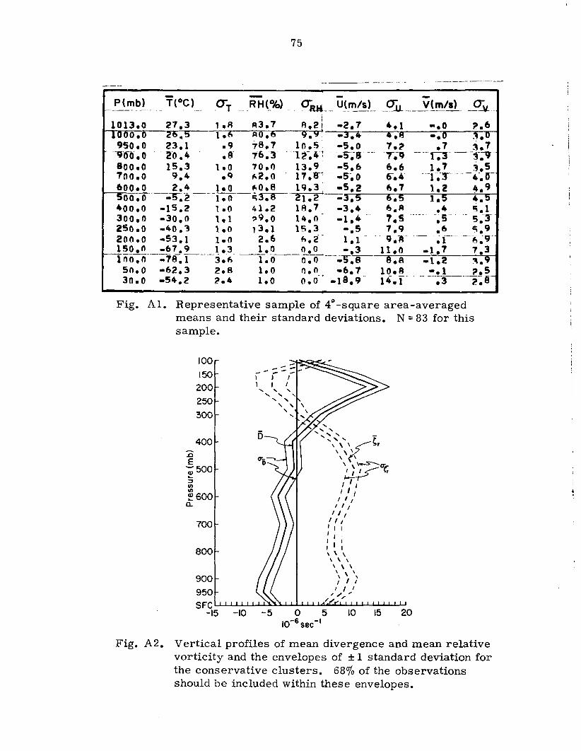
75

- -O""aM __ utm/sL_~ __ H __ ~tm/.) _ _ Qi, __

o. - • ~. 950.0 23.1.9 10.5 -5.0 7.~ .7 ~.7 ~-o-o.o 20,4 .~l -12-.4:-S~-8 ---- "r;9 ---1.3- ----j-~-

800.0 15.3 1.0 70.0 13.9 -5.6 6.6 1.7 3.5 1'00.0 9.4 .q ,,2.0 - l.,.a-~ ----S~O -- 0';.- -----T~T---4-;O-600.0 2.4 1.0 ~0.8 19.3: -5.2 6.7 1.2 4. 9 --SOO~O---T.2 --- -1 • 0 --~3.8-- - 21. 2--';l";~;;;---"":"'.------:1~.:...p-----:4-=.T-I 400.0 -15,2 1.0 41.2 18.7 -3.4 6,A .4 ~.1 300,n -30,0 1,1 ';)9.0 14.0 -1.4 - 7.S -,5- -- 5.3"" 250,0 -40.l 1.0 13.1 1;,3 -.5 7,9 .6 ~.9 200.0 -53.1 1.0 2.6 ~.2 1.1 9.14- ~i--- -~~9-

~~Q.-!.~ ____ ~!,7_,~ ____ ~ .3 ___ t.~ ___ ~ -,3 _-:.1...:;1~.~0=--_-..:.-1. 7 7.3 1no.0 -78.1 3.6 1.0 0.0 --~!).8 8.A -1.2 ,. 50.0 -62.3 2.8 1.0 n.o -6.7 lO.A -.1 ~.5 30.0 -54.2 1?4 1.0 0.0-' _1 9 .9- 14-.1- ---;3----- 2-, A

Fig. AI. Representative sample of 4"-square area-averaged means and their standard deviations. N = 83 for this sample.

100

150 \

200

250

300

400 :c E

-;;; 500 :; en en ~600 a.

700

800

900

950 SFC

-15 -10

... ... ' ...

..... " " -"\""'yCr

\ , \ \ ,

\ \ W-S-a.;

~r. I I I I I I

I I I I I I

I I I I I I I I 1 , , , I I I I \ \ \ , \ \

\ \ \ , \ \

; I ) I I I /" .­

/ '" 10 15 20

Fig. A2. Vertical profiles of mean divergence and mean relative vorticity and the envelopes of ± 1 standard deviation for the conservative clusters. 68% of the observations should be included within these envelopes.

76

where a l' Nl and a 2' N2 are the respective standard deviations and

sizes of the two samples. In the particular case of computing the

deviations for the profiles of divergence or relative vorticity, the

above equation is adapted such that

2 a

n

N n

222 a cr cr +_s_+~+~

N N N sew

where the subscripts n, s, e, w, denote, respectively, the samples

north, south, east, and west of the 4° - square center box for which

the divergence or relative vorticity computation is being made.

These small deviations about the mean relative vorticity and

divergence profiles lend further confidence to the quantitative reason-

ing based on the mean vorticity and divergence profiles of Figs. 27

and 37.

77

REFERENCES

Bohan~ W. A.) 1968: Tropical Pacific cbud patterns, ESSA digital product. 1967 (WAB 196). 16mrr ... ~'~~~-:-.i. prepared by the Walter A. Bohan Company~ Park Ridge, Ii.l:nois.

Chang, C. -P., 1970: Westward propagaLing cloud patterns in the tropical Pacific as seen from time-composite satellite photo­graphs. J. Atmos. Sci., 27, 13S-138.

Chang, C. -Po ~ V. F. Morris, and J. M. Wallace, 1970: A statis­tical study of easterly waves in tt.e western Pacific: July­December 1964. {. Atmos. Sci •• 27, 195-201.

Charney, J. G., 1958: On the formation of tropical depressions. Paper presented at the First Technical Conference on Hurricanes and Tropical Meteorology, Miami, Florida.

Charney, J. G. and A. Eliassen, 1964: On the growth of the hurri­cane depression. J. Atmos. Sci.. 21, 68-75.

Elsberry~ R., 1966: On the mechanics and thermodynamics of a low-level wave on the easterlies. Atmos. Sci. Paper No. 101. Colorado State Dniv., 31 pp.

Fett, R. W., 1964: Tiros photographs and mosiac sequences of ::'opical cyclones in the western Pacific during 1962. Meteorological Satellite Lab. Rept. No. 32, D. S. Weather Bureau, National Weather Satellite Center, Washington~ D. C.

Frank, i\. L., 1969: The "Inverted V'I doud pattern - an easterly wave? Mon. Wea. Rev., 97, 130-140.

Fra[H(, ::\". L., 1970: Atla:1tic -~::'opical system.:'> of 1969. Mon. Wea. Rev., 98~ 307-311,;,.

Frank, N. L., :::",-_,-, ~:...~. ~\i. J or~: . .:'>orl~ 1. ~)6 ~j: 'v' c,,"-cical clG'u-: ~ystems

over the -.::..~opical A'dant';'c duri:.g -cL"t' :.. 967 hurY'ic:::":'L: season. ~\/;:O{l. Wea. riev. ~ 97~ 1.24-:"2~:.

J:,~:,~·~z .. 5., L. ~~"\v ~::\i·oer"LJo arJ.L _.;. .. r~ .... ~-:::.._ .. (;.~ ___ ._ 36: SO::l.e :'1.'1i"erenees

=':..~,::;:;'.,. ':)(·-,,· .. 2~~~~'::~~ ~)ic~~res of LrOiJ:'(:~.l.. (1:":;. .. ~ ... ··bance~. :.\/t:on ...... lilea. Rev., S:2. :2):"-236.

78

Fujita, T., K. Watanabe, and T. Izawa. 1969: Formation and structure of equatorial anticyclones caused by large-scale cross-equatorial flows determined by ATS-1 photographs. ~ Appl. Meteor., 8, 649-667.

Gangopadhyaya, M., and H. Riehl, 1959: Exchange of heat, mois­ture' and momentum between hurricane Ella (1958) and its environment. NHRP Report No. 29, 12 pp.

GARP report on the first session of the study group on tropical disturbances (Madison, Wis., 21 October - 8 November 1968), Joint GARP Organization Committee, WMO.

Gray, W. M., 1967: The mutual variation of wind, shear, and baroclinicity in the cumulus convective atmosphere of the hurricane. Mon. Wea. Rev., 95, 55-73.

Gray, W. M., 1968: Global view of the origin of tropical disturbances and storms. Mon. Wea. Rev., 96, 669-700.

Hayden, C. M., 1969: Objective dimensions of Pacific cloud clusters. Paper presented at the 50th Annual Meeting of the American Geophysical Union, Washington, D. C.

Malkus, J. S., and H. Riehl, 1964: Cloud Structure and Distri­butions over the Tropical Pacific Ocean. Berkeley and Los Angeles, Univ. of California Press, 229 pp.

Mendenhall, B., 1967: A statistical study of frictional wind veering in the planetary boundary layer. Atmos. Sci. Paper No. 116, Colorado State Univ., 57 pp.

Oliver, V. J., and R. K. Anderson, 1969: Circulation in the tropics as revealed by satellite data. Bull. Amer. Meteor. Soc., 50, 702-707.

Palmer, C. E., 1952: Tropical Meteorology. Quart. J. Roy. Meteor. Soc., 78, 126-164.

Riehl, E., 1945: Waves in the easterlies ::-::.nd The polar front in the tropics. Dept. of Meteorology. Un .. v. of Chicago, Misc. ~={ept. 17, 79 pp.

LL~,:[-.~ .. :..., 1854: ·J..~ropical. Meteo~ology. New York, McGraw-Hill, 392 pp.

79

Riehl~ H., and J. S. Malkus, 1958: On the heat balance in the equatorial trough zone. Geophysica, 6, 503-538.

Riehl~ H. ~ and J. S. Malkus, 1961: Some aspects of hurricane Daisy, 1958. TeHus, 13,181-213.

Sadler, J. C., 1962: Utilization of meteorological satellite cloud da ta in tropical meteorology. Proc eedings of the First International Symposium on Rocket and Satellite Meteorology~ Washington, D. C.

Sadler, J. C., 1966: The easterly wave - the biggest hoax in tropical meteorology. Paper presented at the seminar at the National Center for Atmospheric Research, Boulder" Colorado, August 8-12.

Simpson, J., M. Garstang, E. J. Zipser, and G. A. Dean, 1967: A study of a non-deepening tropical disturbance. ~. Appl. Meteor., 6, 237-254.

Simpson. J., and V. Wiggert, 1969: Models of precipitating cumulus towers. Mon. Wea. Rev., 97, 471-489.

Simpson, R. H., N. Frank, D. Shideler, and H. M. Johnson, 1968: Atlantic tropical disturbances, 1967. Mon. Wea. Rev., 96, 251-259.

Simpson, R. H., N. Frank, D. Shideler, H. M. Johnson, 1969: Atlantic tropical disturbances of 1968. Mon. Wea. Rev., 97, 240-255.

Spiegel. M. R. ~ 1961: Theory and Problems of Statistics. New York, Schaum Publishing Co., 359 pp.

Wallace, J. M., and C. -Po Chang, 1969: Spectrum analysis of large-scale wave disturbances in the tropical lower tropo­sphere. J. Atmos. Sci., 26, 1010-1025.

Weinstein, A. : .• and L. G. Davis, 1968: A parameterized numeri­cal model of cumulus convection. Rept. No. 11 to NSF. Pennsylvania State Dniv., 44 pp .

Yanai, M., 1961: Met. Soc.

.:\ detailed analysis of typhoon formation. J. .je:.Pd.:1, Sere II~ 39, 187-214.

80

Yanai, M., 1963: A preliminary survey of large-scale disturbances over the tropical Pacific region. Proceedings of the III Technical Conference on Hurricanes and Tropical Meteorology, Mexico City.

Zipser, E. J., 1969: The role of organized unsaturated convective downdrafts in the structure and rapid decay of an equatorial disturbance. J. Appl. Meteor., 8, 799-814.