A statistical description of verbal learning

PSYCHOMETR1KA--VOI~. 17, NO. 4 DECEMBER, 1952

A S T A T I S T I C A L D E S C R I P T I O N OF VERBAL L E A R N I N G *

GEORGE A. ~/IILLEB. AND W I L L I A M J. MCGILL

MASSACHUSETTS INSTITUTE OF TECHNOLOGY

Free-recall verbal learning is analyzed in terms of a probability model. The general theory assumes that the probabiliW of recalling a word on any trial is completely deternfined by the number of times the word has been recalled on previous t~als. Three particular cases of this general theory are examined. In these three cm~es, specific restrictions are placed upon the relation between probability of recall and number of previous recalls. The application of these special cases to typical experimental data is illustrated. An interpretation of the model in terms of set theory is suggested but is not essential to the argument.

The verbal learning considered in this paper is the kind observed in the following experiment: A list of words is presented to the learner. At the end of the presentation he ~n'ites down all the words he can remember. This procedure is repeated through a series of n trials. At the present time we are not prepared to extend the statistical theory to a wider range of experimental procedures.

The General Model

We shall assume that the degree to which any word in the test matel~al has been learned is completely specified by the number of times the word has been recMled on preceding trials. In other words, the probability tha t a word will be recalled on trial n -t- 1 is a function of k, the number of times it has been recalled previously. (Symbols and their meanings are listed in Appendix C at the end of the paper.)

Let the probability of recall after k previous recalls be symbolized by rk . Then the corresponding probability of failing to recall the word is 1 -- rk . When a word has been recalled exactly k times on the preceding trims, we shall say that the word is in state Ak. Thus before the first trial all the words are in state Ao ; tha t is to say, they have been recalled zero times on previous trials. Ideally, on the first trial a proportion ro of these words is recalled and so passes from state Ao to state A~ . The proportion 1-- ro is not recalled and so remains in state Ao . On the second trial the

*This research was facilitated by the authors' membership in the Inter-University Summer seminar of the Social Science Research Council, entitled Mathematical Models for Behavior Theory, held at Tufts College, June 28-August 24, 1951. The authors are especially grateful to Dr. F. Mosteller for advice and criticism that proved helpful on many different occasions.

369

372 PSYCHOMETRIKA

When this result is subst i tuted into the expression for pn÷~, we have

k - O k ~ O

= ~ 7"~p(Ak , n), k = 0

which is the desired result. The asymptot ic behavior of the model as n increases without limit can

be deduced from the general solution (2). First consider the case in which one or more of the transitional probabilities rk is zero. All the words s tar t in s tate Ao and have a positive probabil i ty of moving along to states A~ , A2 , etc., up to the first state, Ah, with zero transitional probabili ty, rh = 0. There the words are t rapped; eventually all the words are recalled exactly h times and cannot be recalled again. This fact can be seen from (2): I f r, > 0, then all the terms (1 - r,) ~ in (2) go to zero as n --* ~ . Thus p(Ak, n) goes to zero for k < h. For k > h, the product in front of the summat ion mus t include rh = O, and so p(A~, n) = 0 for k > h. When k = h, however, (1 - rh) ~ = (1 - O) ~ = 1, and so this term in the summation of (2) does not go to zero. Instead, when ~'A = 0 and r~ > 0 for i < h,

T O T 1 • . . T h _ 1

lim p(Ah, n) = (to -- rh)(r~ -- rh) " ' " (r,_~ -- rh) = 1 .

The recall score, p~,~ , then approaches zero as an asymptote ; from (5),

l im 0~+1 = ~ rk[lim p(Ak 1 n)] = O,

since the probabil i ty a t the asymptote is concentrated a t s ta te Ah , and for this s tate r~ =- 0. This case is of little interest for an acquisition theory, since the asympto te of the learning curve is a t zero. Therefore, in what follows, we shall be concerned only with the case in which all the rk are different and greater than zero.

If all the transitional probabilities rk are greater than zero, t tmn from (2) we see tha t as n approaches infinity all the terms in the summat ion go toward zero for all finite values of k. Consequently the sum of the p(Ak , n) can be made as near zero as we please for any finite k by selecting a large enough value of n. In the limit, therefore, the probabil i ty of any finite number of recalls is zero. Since the sum of the p(Ak , n) must equal unity, almost all the probabil i ty comes to be concentrated in state A® and we have for the limit when all rk > 0,

p ( A ® , ¢o) = 1.

GEORGE A. MILLER AND WILLIAM J . MCGILL 3 7 ~

W e are now able to show t h a t a word in s t a t e Ak has p r o b a b i l i t y one of mov ing to s t a t e Ak÷~ , if the l ea rn ing process is con t i nued indef in i te ly . Th i s h a p p e n s because a lmos t all words even tua l ly reach s t a t e A® . T h u s we can wri te , for the p r o b a b i l i t y of l eav ing s t a t e Ak on some t r ia l ,

m

n ~ k

or,

an a s y m p t o t e as k --* ~ . t ions on the rk:

~-'~ p(Ak , n) -- for rk > 0. 1

n ~ k ~ k

In al l the cases we shal l cons ider in th is p a p e r the va lue of rk will a p p r o a c h W e are in t e res t ed in p lac ing the fol lowing res t r i c -

Tk ~ T i

r~ > O,

l i m r k = m <: 1.

The first two cond i t ions insure t h a t p(Ak , n) goes t o w a r d zero for f inite k and large n. The th i rd condi t ion p rov ides the a s y m p t o t i c va lue of r , for infini te k. I n the s u m m a t i o n for the l imi t ing va lue of p . + , , all t e rms are zero ou t to inf ini ty , and so we have

l im pn+, = mp(A® , ¢~) = m. (5')

I n o the r words, if we assume t h a t m is the a s y m p t o t i c va lue of rk as k --~ co, then m is also the a s y m p t o t i c va lue of pn+~ as n -~¢~.

In the special cases d iscussed below, a res t r i c t ion is p laced upon the va lue of Tk in the form of the l inear difference equat ion ,*

vk+l = a + ark , (6)

w h e r e 0 < a < l a n d 0 < a < 1 -- a. T h e l imi ts for a have been chosen so t h a t rk÷ , is b o u n d e d be tween zero and one and , s ince we are in t e res t ed in acquis i t ion , so t h a t rk÷ , _> r k .

Cons ide r t he fol lowing developmet~t of (5):

n+!

k=O

*We have tried to observe the convention tha t parameters are represented by Greek letters and statistical est imates are represented by Roman letters. In the case of a and m, however, we have vioh~ted this convention in order to make our symbols coincide with those used by other workers. The symbols m, a, , , and p were originally proposed by Bush and Mosteller.

374 PSYCHOMETRIK&

Now substitute for p(Ak , n + 1) according to (1):

n+~, n ÷ !

p..2 = ~ rkp (A , , n)(l -- r,) + ~ r~p(Ak_,, n)r~_, k - O k~O

= P.+l -- ~ , r :p(Ak, n) -{- ~ , ~,+~rkp(A,, n). k - O k - O

Next we substitute for r~+x according to CO):

o . ÷ . = o . ÷ , - , n) + (a + , n) k - O k - O

k - O

= (I + a)p.÷, -- (1 -- a)E(r~,, n + 1), (7)

where E(r~ , n + 1) is the second raw moment of the rk (as p.÷l is the first raw moment) for trial n + 1.

Restriction (6) brings the system into direct correspondence with a special case of the theory developed by Bush and Mosteller. In their termi- nology, an operator Q1 is applied to the probability of response, p, to give a, + a~p as the new probability whenever a trial is successful. A second operator Q2 is applied to give a2 + a2p whenever a trial is unsuccessful. In the present application of this more general theory, Qz is preserved intact by restriction (6), but Q2 is assumed to be the identity operator. That is to say, a2 is zero and a2 is unity, so Q2p = p- In the present application, an unsuccessful trial consists of the omission of the word during recall. I t seems reasonable to assume that the non-occurrence of a word has no effect upon its probability of occurrence on the next trial. How successful this simple assumption is will be seen when we examine the data.

Analysis of the Data

At the end of the experiment the experimenter has collected a set of word lists--the words recalled by the learner on successive trials. These recall lists will usually contain a small number of words that did not occur in the presentation. These spontaneous additions by the learner are of some interest in themselves, but we shall ignore them in the present discussion.

We would like to use the data contained in the word lists to obtain an estimate of p.+, in (5). We shall refer to the estimate as r.+l . There are, we suppose, N words provided by the experimenter as learning material in the experiment. I t seems reasonable to assume that under certain conditions these words are homogeneous. :By this we imply that the responses to all of the words in state Ak may be considered arS estimates of the same transitional probability of recall, rk •

GEORGE A. M I L L E R AND W I L L I A M J . M C G I L L 375

We can then define a convenient statistic,

1 ~ ~ X , . , . . ÷ , . (8)

The numbers, X,.~...I , are either zero or one. The subscripts k and n -{- I have the same meaning tha t we have at tached to them previously. They indicate tha t we are looking at an event tha t occurs on trial n q- 1 to a word in state Ak . The first summation is carried out over i, the experimental words, with k fixed to show that we count the number of words in each state. The rules tha t determine whether an X,.~.~.I is zero or one are straight- forward. The X, .k. . . , are zero for all words not in state A, when summing on i. They are zero for any word in state A~, if a recall fails to occur on trial n q- 1. Lastly the X,.k..** are 1 for any word in state A , , provided tha t a recall occurs on trial n q- 1. The second summation extends over k, the various states. This summation goes only up to n because our reference point for determining the number of states is trial n. These rules determine r..~ as the proportion of correct responses to the N experimental words on trial n -{- 1.

To show that r . . , is unbiased we observe that

E ( r . . , ) = ~ , - ,

The expectation of any X,.,,.** in state Ak is rk . Thus the expectation of the sum in the brackets is N.r , . p (A , , n). Substituting this into the expression for E( r . . l ) , we find

E(r~.~) = ~ rkp(Ak , n), k - O

E(r.+~) = p~+,. (9)

The sampling variance of r~+, around p.+~ is determined by the variances of the various X~.k..+~ around the transitional probabilities, 7~.

,± ) V a t ( r . , , ) = ~ V a r X , . ~ . ~ ÷ , .

The variance of any X,.,..+, in state A, is binomial and is given by r , ( l - r~). The variance of Y~,~a X,.,..** thus becomes N p(Ak, n)r , (1 -- rk). Substi tut- ing this into the expression for Var (r.**), we obtain

1 n

p(A, n)rk(1 -- v,). (I0) V a r (r .+, ) = ~ .

I t should be noted that this variance is never larger than the binomial variance

1 p . . , • (1 - p .+ , ) ,

376 PSYCHOMETRIKA

since the binomial variance includes in addition to (10) a term that depends on the variance of the r~ around p.+~ ,

Var(r.+,) p . + , ( 1 - p.+,) 1 { ~ 2 A , 2 } (10') = N - - N Tkp( k n ) - p.+, . k = 0

In order to apply the general theory we must obtain estimates of the transitional probabilities, Tk • NOW rk is the probability of moving from state Ak to Ak÷~ and is assumed to be constant from trial to trial. After trial n a certain number of words, Nk. . , are in state A~. Of these N~.. words, some go on to Ak+~ and some remain in Ak on trial n q- 1. The fraction tha t moves up to Ak+~ provides an estimate of rk on that trial. Therefore, on every trial we obtain an estimate of rk • Call these estimates tk..÷~ • Then

N

Z Xl.k,n+l

lk.,+l : '=~Nk..

If N~., is zero, no estimate is possible. Next we wish to combine the t~.,+~ to obtain a single estimate, tk , of

the transitional probability, rk • The least-squares solution, obtained by minimizing (tk.,+~ - rk) 2, is the direct average of the tk .... ~ . This est imate is unbia~d, bu t it has too large a variance because it places undue emphasis upon the t,.,+a that are based on small values of N~ . . . . We prefer, therefore, to use the maximum-likelihood estimate,

Y]~ IVk,nlk,n+ t n

t, -- Z Nk., ' (11) n

which respects the accuracy of the various tk.,÷~ • For example, after trial 7 there may be 10 words in state A3 . Of these

10, 6 are recalled on trial 8. This gives the estimate t3.s = 6/10. Every trial on which N3,, ~ 0 provides a similar estimate, t3.,÷l • The final estimate of r3 is obtained by weighting each of these separate estimates according to the size of the sample on which it is based and then averaging. This pro- eedure is repeated for all the r , individually as far as the data permit.

The t~.,+~ are also useful to check the basic assumption tha t r , is independent of n. If the tk,,+~ show a significant trend, this basic assumption is violated.

The Simplest Case: One Parameter

The computation of p(Ak , n) from (2) for the general case is exceedingly tedious as n and k become moderately large. We look, therefore, for a simple relation among the Tk of the form of restriction (6). The first case that we

G E O R G E A. M I L L E R AbID W I L L I A M g . M C G I L L 3 7 7

shall consider is

T O ~ a,

~k+, = a + (1 - a ) ~ k . (12)

In this form the model contains only the single parameter, a. The solution of the difference equation (12) is

rk = 1 -- (1 -- a) ~+'. (13)

The interpretation of (13) in set-theoretical terms runs as folIows: On the first presentation of the list a random sample of elements is conditioned for each word. The measure of this sample is a, and it represents the probability, ro, of going from state A,, to state Al . If a word is not recalled, no change is produced in the proportion of conditioned elements. When a word is recalled, however, the effect is to condition another random sample of elements, drawn independently of the first sample, of measure a to that word. Since some of the elements sampled at recall will have been previously conditioned, after one recall we have (because of our assumption of independence between successive samples):

Elements conditioned~ [Elements conditioned~ _ ( Common ) during presentation / -t- \ during the recall / elements

= a d - a - a 2 = 1 - ( 1 - a ) 2.

This quanti ty gives us the transitional probability r~ of going from A~ to A2, from the first to the second recalt. The second time a word is recalled another independent random sample of measure a is drawn and conditioned, so we have

r2 = [1 - (1 - a ) 2] d - a - a [ l - (1 - a ) 2] = 1 - (1 - a ) a.

Continuing in this way generates the relation (13). With this substitution the general difference equation (1) becomes

p(A~, n + 1) = p(A,, n)(1 - a) ~+t d- p(Ak_,, n)[1 -- (1 -- a)~].

The solution of this difference equation can be obtained by the general method outlined in Appendix A or by the appropriate substitution for rk in (2). The solution is

p(Ao, n) = (1 - a)', k - 1

p(A,, n) = (1 -- a) "-k I~ [1 -- (1 -- a)'-']. (14) i - -0

From definition (5) it is possibie to obtain the following recursive ex-

37g PSYCHOMETRIKA

pression for the recall on trial n -}- 1 (see Appendix B):

p. . : = a -}- (1 - a)[1 - (1 -- a ) " ] p , , .

The variance of the recall score, r,+~ , is

1 V a r (to+,) = (po+2 - p.+,).

( 1 5 )

(16)

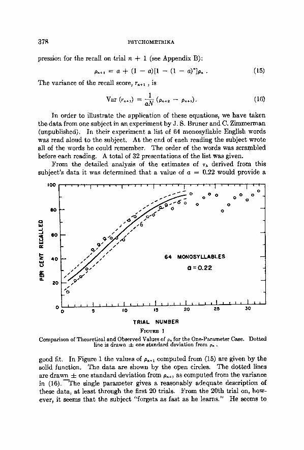
In order to illustrate the application of these equations, we have taken the data from one subject in an experiment by J. S. Bruner and C. Zimmerman (unpublished). In their experiment a list of 64 monosyllabic English words was read aloud to the subject. At the end of each reading the subject wrote all of the words he could remember. The order of the words was scrambled before each reading. A total of 32 presentations of the list was given.

From the detailed analysis of the estimates of ~k derived from this subject 's data it was determined tha t a value of a = 0.22 would provide a

100

eO

60

40

20

' ' " ~ ' t . . . . I . . . . I . . . . t ' ' ~ ' ' I . . . . 'l" ' '

, . , ~ ~ 0 0 O 0 0 0 0 0 0 O 0 0

_ / /

_ t , ~ g / . s" 64 MONOSYLLABLES

~ - ~ o ~ " 0 - 0 . 2 2

/ ~ ° , ~ j I I , , , i 1 , , , , I , , , , I , , , , I , , , , 1 ' ' 0 5 I0 15 20 25 30

o

.J

.J <1 ¢J k~J ~r

laJ u ¢¢

a .

TRIAL NUMBER

FIGURE 1

Compar i son of Theoretical and Observed Values of p. for the One-Parameter Case. Do t t ed line is d rawn 4- one s t andard deviation from p . .

good fit. In Figure 1 the values of p,+l computed from (15) are given by the solid function. The data are shown by the open circles. The dot ted lines are drawn 4- one standard deviation from pn÷~ as computed from the variance in (16).---The single parameter gives a reasonably adequate description of these data, at least through the first 20 trials. From the 20th trial on, however, it seems tha t the subject "forgets as fast as he learns." He seems to


reach an asymptote somewhat below the theoretical value at unity. The introduction of an asymptote less than unity will be discussed in connection with the three-parameter case.

f o k=3

o

6 0

V \o 4 o

1 J i J J 1 I J I , | ? ? o ~ ' ~ " ~ - - ~ , i I 0 0 5 I0 15 20

TRIA l . NUMBER

Fxotm~ 2

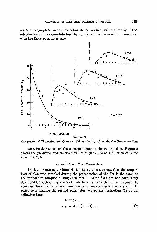
C o m p a r i s o n o f T h e o r e t i c a l a n d O b s e r v e d V a l u e s o f p(Ak, n) f o r t h e O n e - P a r a m e t e r C a s e

As a further check on the correspondence of theory and data, Figure 2 shows the predicted and observed values of p(Ak , n) as a function of n, for k = 0 ,1 ,2 ,3 .

Second Case: Two Parameters.

In the one-parameter form of the theory it is assumed that the proportion of elements sampled during the presentation of the list is the same as the proportion sampled during each recall. Most data are not adequately described by such a simple model. At the very least, then, it is necessary to consider the situation when these two sampling constants are different. In order to introduce the second parameter, we phrase restriction (6) in the following form:

TO ~ PO

rk+l = a "4- (1 -- a)rk, (17)

380 PSYCHOMETRIKA

where Po is the propor t ion of e lements condi t ioned dur ing the presentat ion. The solution of this difference equat ion can be wr i t ten

T~ = 1 -- (1 -- p0)(l -- a) k. (18)

On the first presenta t ion of the list a r a n d o m sample of measure Po is condi t ioned to every word. When a word is recalled, a r a n d o m sample of measure a is drawn and condit ioned. After one recall, therefore, the measure of condit ioned elements is

• ~ = P o - { - a - - apo = 1 -- (1 -- po)(1 -- a).

After two recalls the measure of condit ioned elements is

~'2 = [I -- (1 - po)(1 -- a)] -]- a - a[1 - (1 - po)(1 - a)]

-- 1 - (l - p0)(1 - a) 2.

Cont inuing in this way generates the relation (18). Wi th this subst i tu t ion the general difference equa t ion (1) becomes

p(A~, n "k 1) = p ( A k , n)(1 -- po)(1 -- a) k

q- p(Ak_~, n)[1 -- (1 -- po)(1 -- a)~- ' ] . (19)

The solution of (19) is

p(Ao , n) = (1 - p0) ",

~ _ I . k - _ _ ( . 1 - p ~ ) ( 1 - a ) ' ] [ 1 - (1 - o F - ' ] p(A~ , n ) = ( 1 - - po) "-~ , -o I - ( 1 - - a) '+1 ( 2 0 )

W h e n P0 = a, (20) reduces to (14). The recursive form for the recall now becomes (see Appendix B)

p,÷l = po + (1 -- po)[1 -- (I -- a ) ' ]p . • (21)

T h e var iance of r.+l is

1 Var (r.+,) = a N (p.+2 -- p .÷ , ) - (22)

In order to illustrate the application of these equat ions we have selected two sets of data . The first set was collected by Brune t and Zimmerman. A list of 32 monosyl labic words was read aloud. At the end of each reading the subject wrote all of the words he could remember . The order of the words was scrambled before every reading. A total of 32 presenta t ions of the list

was given. F r o m the analysis of the tk calculated for this par t icular subject i t was

found tha t a = 0.10 and po = 0.27 gave a good descript ion of the data . I n Figure 3 the values of p~+~ compu ted f rom (21) are shown b y the solid function. The da t a are given b y the open circles. The do t t ed lines are d rawn

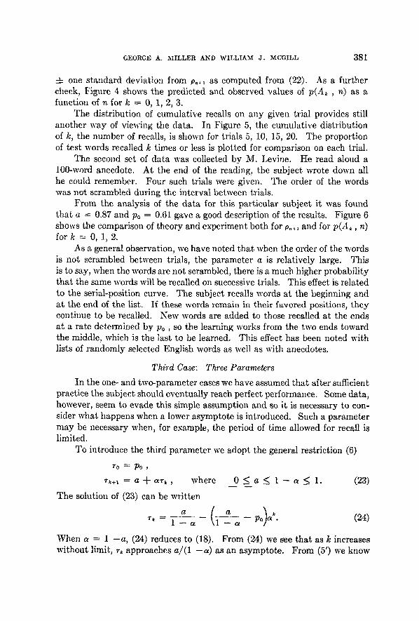
GEORGE A. ~ I I L L E R AND W I L L I A M J . M C G I L L 381

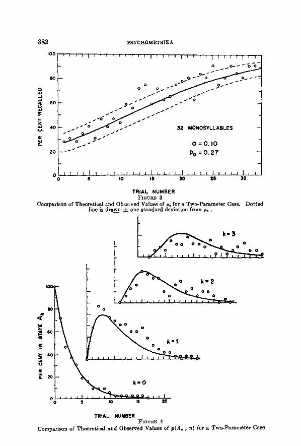
=t= one standard deviation from p,~l as computed from (22). As a further check, Figure 4 shows the predicted and observed values of p(Ak , n) as a function of n for lc = 0, 1, 2, 3.

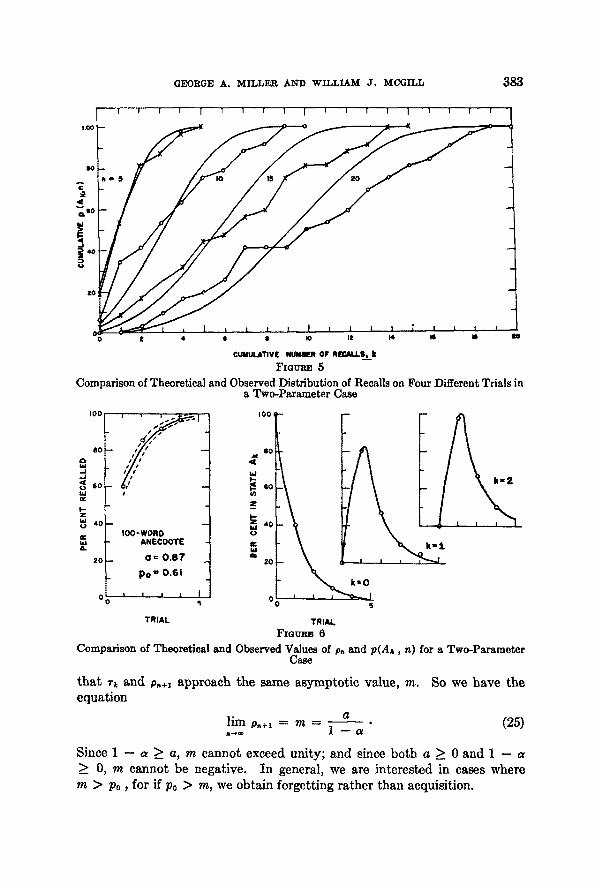
The distribution of cumulative recalls on any given trial provides still another way of viewing the data. In Figure 5, the cumulative distribution of k, the number of recalls, is shown for trials 5, 10, 15, 20. The proportion of test words recalled k times or less is plotted for comparison on each trial.

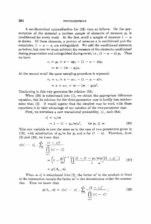
The second set of data was collected by M. Levine. He read aloud a 100-word anecdote. At the end of the reading, the subject ~,n'ote down all he could remember. Four such trials were given. The order of the words was not scrambled during the interval between trials.

From the analysis of the data for this particular subject it was found tha t a -- 0.87 and Po = 0.61 gave a good description of the results. Figure 6 shows the comparisoa of theory and experiment both for p,+, and for p(Ak, n) f o r k = 0 , 1 , 2 .

As a general observation, we have noted that when the order of the words is not scrambled between trials, the parameter a is relatively large. This is to say, when the words are not scrambled, there is a much higher probability that the same words will be recalled on successive trials. This effect is related to the serial-position curve. The subject recalls words at the beginning and at the end of the list. If these words remain in their favored positions, they continue to be recalled. New words are added to those recalled at the ends a t a rate determined by po, so the learning works from the two ends toward the middle, which is the last to be learned. This effect has been noted with lists of randomly selected English words as well as with anecdotes.

Third Case: Three Parameters

In the one- and two-parameter cases we have assumed that after sufficient practice the subject should eventually reach perfect performance. Some data, however, seem to evade this simple assumption and so it is necessary to consider what happens when a lower asymptote is introduced. Such a parameter may be necessary when, for example, the period of time allowed for recall is limited.

To introduce the third parameter we adopt the general restriction (6)

TO ~ P0

r~+~ = a ~ ~r~ , where 0 ~ a _~ 1 -- a ~ 1. (23)

The solution of (23) can be writ ten

a ( a ) r k - 1 - - ~ 1 ~ Po a k. (24)

When a = 1 --a, (24) reduces to (18). From (24) we see that as k increases without limit, r , approaches a/(1 --a) as an asymptote. From (5') we know

382 PSYCHOM~I'RIKA

e¢

s o

,~. 4o

Q.

100 " ~ ~ ~ ! ~" ~ ~ ~""~ ~ r ' J z ' ' l ' 1 1 1 '1 I i ~ ! t ] t I l ' t l ' " t !

L- o o - - - "6 - o - .

O .. 0 "O''O"

. s O ' ' ~ O ~ ~ d ,.,, '~ ~ '~ -

" . . ~ . " " " ~ 32 MONOSYL.LABL.ES

" O f O . . " " " - o . . , - O = O . I O

20 - - - " Po = O . 2 7

0 J 1 J I ] ~ I I I I I I i | ] 1 L t ! [ I J I J I i I I I ] I I 0 5 ~0 15 2 0 | 6 3 0

T R I A L N U M B E R FIGURE 3

Comparison of Theoretical and Observed Values of p~ for a Two-Parameter Case. Do t t ed ]ine is drawn -4- one s tandard deviation from p~.

f k-S

IOoq

O 8 0 O

I~ o o

4O o . . . . . . " . . . . . . . .

k - O

o 5 IO 18 gO

o k " 2

o o

T R I A L N U M B E R Fzow~ 4

Comparison of Theoretical and Observed Values of p(A~, n) for a Two-Parameter Case

GEORGE A. M I L L E R AND W I L L I A M J . M C G I L L 3 8 3

t.O0 - -

8 O

~'° _1

zO

% ~ i I I I 1 t I I ~ I I | ! I l I O~" ~ 2 4 6 II I0 llt 14 141+ II 20

cmmu~mvE .um.~ OF . m ~ . s _ k

Fzouv.E 5 Comparison of Theoretical and Observed Distribution of Recalls on Four Different Trials in

a Two-Parameter Case

80

so

4O

2O

,oo , ' '"'"" " . ~ 1 , co ¢ , s ;

/1~ ss / -

' i IO0-WORD

- ANECDOTE

O f 0 . 8 7

P o " 0.61

t ! i | 1

8O

tU

Z

,.;, ,o f.)

eC kLJ t

ZO

T R I A L

0 5

T R I A L

F m m ~ 6

Comparison of Theoretical and Observed Values of ~ and p(Ak, n) for a Two-Parameter Case

that ~k and p.÷1 approach the same asymptotic value, m. So we have the equation

(25) l i m p , + l = m = 1 - - + + n--~¢o

Since 1 -- a _> a, m cannot exceed unity; and since both a ~ 0 and 1 - a > O, m cannot be negative. In general, we are interested in cases where m > Po, for if Po > m, we obtain forgetting rather than acquisition.

384 PSYCHOMETRIKA

A set-theoretical rat ionalization for (24) runs as follows. On the presentat ion of the material a r andom sample of e lements of measure P0 is condit ioned for every word. At the first recall a sample of measure 1 - a is drawn. Of these elements, a port ion of measure a is condit ioned and the remainder, 1 -- a -- a, are extinguished. We add the condi t ioned e lements as before, bu t now we mus t sub t rac t the measure of the e lements condi t ioned dur ing presenta t ion ~nd extinguished dur ing recall, i.e., (1 - a - a) Po. T h u s we have

r~ = p o ~ - a - - a p o - - ( 1 - - ~ - - a ) p o

= m - - ( m - - p o ) o .

At the second recall the same sampling procedure is repeated:

r. , = r, -{- a - - a t , - - ( 1 - a - - a ) r ,

= a - [ - o ~ r l = m - - ( m - - p 0 ) ~ 2 .

Cont inuing in this way generates the relation (24). When (24) is subst i tu ted into (1), we obtain the appropr ia te difference

equat ion, bu t its solution for the three-parameter case is hard ly less cumber- some than (2). I t would appear t ha t the simplest way to work with these equat ions is to take advan tage of our solution of the two-paramete r case.

First , we int roduce a new transit ional probabil i ty, r;, , such tha t

• '~ = ~ J m

= 1 -- (1 -- p o / m ) a ~', for Po _< m. (26)

This new variable is now the same as in the case of two parameters given in (18), with subst i tu t ion of p o / m for Po and a for (1 - a). Therefore, f rom (2) and (20), we know tha t

1 P ° + P

-k"-

i - 0

m / i - o 1 - - o~ ' ÷ ~

= p ' ( A ~ , n ) .

When m r~ is subs t i tu ted into (2), the factor m k in the produc t in front of the summat ion cancels the factor m k in the denomina tor under the summation. Thus we know tha t

p ( A k , n) = ro'r~' *. • r~'_, ~ ,-(1 -- r,)" , (28) i - 0

I -I (¢~ - ~)

GEORGE A. M I L L E R AND WILLIA.-%I J . M C G I L L 3 8 5

which is the same as p ' (Ak , n) in ( 2 7 ) except for the numera to r under the summat ion . This numera to r can be wri t ten

(1 - - r,)" = [(1 - - m ) + m ( 1 - - r:)]"

= (1 - - m)" - } - n ( 1 - - m ) " - ~ m ( 1 - - r~)

+ ( 2 ) ( 1 - - m ) " - 2 m 2 ( 1 - - r ~ ) ~ + . . . m " ( 1 - v~)". (29)

N o w we subst i tu te this sequence for the numera to r in (28) and sum term by term. When we consider the last term of this sequence we have

, , . . . ~;_, ~ m"(I - rg" T o T 1 k

,.o [ I e ) i=O

which we know from (27) is equal to m"p ' (Ak , n). The next to last term gives

~o~,', . . . ~ , _ , / : n ( l - m ? - ' ( 1 - , ' 3 ''-~

i-O

which we know from (27) is equal to n(1 - re)m"-' p ' ( A k , n -- 1). Proceed- ing in this manner brings us eventual ly to the case where n < k, and then we know the term is zero. Consequent ly , we can write

p(A~ , n) -- m"p ' (Ak , n) + n(1 -- m ) m " - ' p ' ( A k , n -- l) + - . .

+ n - k (1 - m ) " - k m k p ' ( , 4 ~ , k )

W h e n the a sympto t e is un i ty (m --- 1), (29) and (30) reduce to the two- pa ramete r case.

We recall t ha t because of the way in which our probabilit ies were de- fined in (1), (30) can be writte~l as

i~O

3 8 6 P S Y C H O M E T R I K &

Now it is not difficult to find an expression for p.+~ in terms of the o~ computed in the two-parameter case:

p~.~ -- ~ ,-.p(A., n) k - O

= m ~ r~p(Ak, n) k - O

= m m' (1 - - m) r~p ( A ~ , ~). k - O ~ - 0

If we invert the order of summation, we find that

p.+t = m ~ (n)m'(1 - m) ' - ' ~ . r~p ' (A, , i) i - O k - O

- - m) p,+~ i - O

(31) = m

The computation of p~+l by this method involves two steps: first, the values of ' p~+l are calculated as in the two-parameter case with the substitution indicated in (26); second, these values of p.'÷~ are weighted by the binomial expansion of [m + (1 - m ) ] ~ and then summed according to (31).

These computations can be abbreviated somewhat by using an approximation developed by Bush and Mosteller (personal communication). I t is

pn+, = (2 + a + 2aa)p~+, - [a2(1 - ~) + (1 + a)(l + 2aa)]p.

+ 3 (1 - ~2)(1 - a)p'. - 2 (1 - ~ ) ( 1 - ~ ) p ~ . - 3 ( 1 - 2 ) p . p ~ + , ,

(n > 1 ) . (32)

The approximation involves permitting the third moment of the distribution of the rk around p~ to go to zero On every, trial.

The variance of r~+i in the three-parameter ease is

m Var (r.+,) = ~-~ [p~+2 - - (a a t- a)p .÷~]. (33)

This expression for the variance of r .÷ , follows directly from (7) and (10'). I t is easily seen that (10') can be written as follows:

~ 2 A , r~ p( ~ n) = O~+, -- N Var (r .÷,) . (34) k - 0

Substituting (34) in (7) and solving for Vat (÷~÷,) we find that

1 Var (r.+,) - N(1 - a) [p.+2 - (a + a)p.+,],

which, except for notation, is (33). The one-parameter and two-parameter variances (16) and (22) are special cases of this expression.

GEORGE A. MILLER AND WILLIAM J . MCGILL 387

I t is of interest to observe that when the limiting value, m, is substituted in (33) for p,+~ and p , . , , the limiting variance is found to be binomial. That is ,

lim Var (r,+l) - m(1 - m) n~¢o --Y

This reflects the fact, established earlier in (5'), that as n grows very large the variance of the r , around m goes to zero.

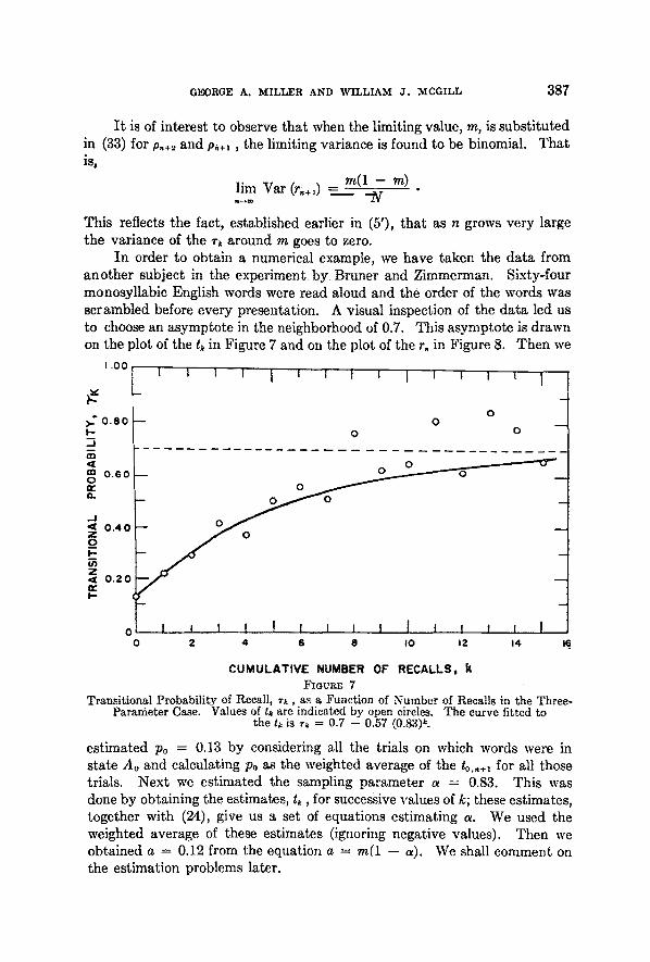
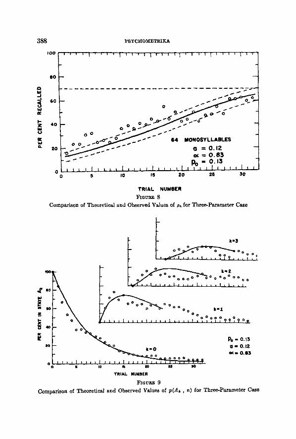
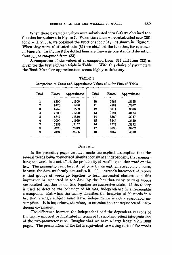
In order to obtain a numerical example, we have taken the data from another subject in the experiment b y Bruner and Zimmerman. Sixty-four monosyllabic English words were read aloud and the order of the words was scrambled before every presentation. A visual inspection of the data led us to choose an asymptote in the neighborhood of 0.7. This asymptote is drawn on the plot of the t, in Figure 7 and on the plot of the r. in Figure 8. Then we

I . 0 0

>." 0 . 8 0 - - I-,.

- J

nn

' ~ 0 . 6 0 - 0 n e

. - I

0 . 4 0 - - 0

I - -

Z

r,- '~ 0 . 2 0 ; I - -

1 | i I I ; 'l ......... I ~ I

0

I I I t l

0 0

0

Transi t ional Probabi l i ty of Recall , r k , as a Funct ion of N u m b e r of Recalls in t he Three- Pa rame te r Case. Values of t , are indicated by open circles. T h e curve f i t ted to

t he tk is T~ --- 0.7 -- 0.57 (0.83)~.

estimated po = 0.13 by considering all the trials on which words were in state Ao and calculating Po as the weighted average of the to.,.~ for all those trials. Next we estimated the sampling parameter a = 0.83. This was done by obtaining the estimates, tk, for successive values of k; these estimates, together with (24), give us a set of equations estimating a. We used the weighted average of these estimates (ignoring negative values). Then we o b t a i n e d a = 0 .12 f r o m t h e e q u a t i o n a = m ( 1 - - a ) . W e s h a l l c o m m e n t o n

the estimation problems later.

0 . . J ! I l l l t i t | I I I I

0 2 4 6 s to tz J4 16

C U M U L A T I V E N U M B E R O F R E C A L L S , It

Fmum~ 7

~ $ 8 Y S Y C H O M E T R I K A

I 0 0

6o

6O

40

a. 2o

o of. - . . -

o . O ' ~ _ . - - " " 64 MONOSYLLABLES O o ~ . .~ '~ ~ ~ ' 0 ~,.~-- " ~

- =o. ,z -0 ~ - " 8 . ~ - o ~ = O . 3

0 I I I 0

D O f f 0 . 1 3 ~ I I l i I t , , I j 1 , t , , 1 t I s , I , I t | J i l l

5 go IS 20 Z8 30

TRIAL NUMBER F : o u ~ 8

Comparison of Theoretical and Observed Values of ~ for Three-Parameter Case

f k-3 O ° 0 ~ 0 0 0 ° ¢

I ~ s • • i i I • i

,O l - \ ~ \ o ° -

f y o ~ ° o O o o o o o ~J l,,l,llilll~ ,I [,~l,,,,J~??J? • 4O

I "% p. - o.,3 "I- ~ k-o o.. o.,2

F ~ o o - - o . .

o S ~ m I0 U I0

TRIAl. NUMBER

Fz~u~s 9

Compsrison of Theoretical and Observed Values of p(Ah, n) for Three-Parameter Case

GEORGE A. MILLER AND WILLIAM J . MCGILL 389

When these parameter values were substituted into (24) we obtained the function for 7k shown in Figure 7. When the values were substituted into (28) for k = 1, 2, 3, 4, we obtained the functions for p(Ak, n) shown in Figure 9. When they were substituted into (31) we obtained the function, for p. shown in Figure 8. In Figure 8 the dotted lines are drawn 4- one standard deviation from p. , as computed from (33).

A comparison of the values of p~ computed from (31) and from (32) is: given for the first eighteen trials in Table 1. With this choice of parametera the Bush-Mosteller approximation seems highly satisfactory.

TABLE 1

Comparison of Exact and Approximate Values of ~ for First 18 Trials

Trial Exact Approximate Trial Exact Approximate

1 .1300 .1300 2 .1426 .1426 3 . ] 559 .1559 4 .1700 .1700 5 .1847 .1846 6 .2ooo .1999 7 .2159 .2157 8 .2323 .2319 9 .2491 .2486

10 .2663 .2655 11 .2837 .2827 12 .3014 .30O0 13 .3191 .3174 14 .3369 .3347 15 .3546 .3520 16 .3722 .3692 17 .3896 .3862 18 .4067 .4030

Discussion

In the preceding pages we have made the explicit assumption that the several words being memorized simultaneously are independent, that memor- izing one word does not affect the probability of recalling another word on the list. The assumption can be justified only by its mathematical convenience, because the data uniformly contradict it. The learner's introspective report is that groups of words go together to form associated clusters, and this impression is supported in the data by the fact that many pairs of words are recalled together or omitted together on successive trials. If the theory is used to describe the behavior of 50 rats, independence is a reasonable assumption. But when the theory describes the behavior of 50 words in a list that a single subject must learn, independence is not a reasonable assumption. It is important, therefore, to examine the consequences of intro- ducing covariance.

The difference between the independent and the dependent versions of the theory can best be illustrated in terms of the set-theoretical interpretation of the two-parameter case. Imagine that we have a large ledger with 1000 pages. The presentation of the list is equivalent to writing each of the words

390 PSYCHOMETRIKA

at random on 100 pages. Thus po = 100/1000 -- 0.1. Now we select a page at random. On this page we find written the words A, B, and C. These are responses on the first trial. The rule is tha t each of these words must be writ ten on 50 pages selected at random. Thus a = 50/1000 = 0.05. With the independent model we would first select 50 pages at random and make sure tha t word A was written on all of them, then select 50 more pages independently for B, and 50 more for C. With a dependent model, however, we could simply make one selection of 50 pages at random and ~ i t e all three words, A, B, and C, on the same sample of 50 pages. Then whenever A was recalled again it would be likely that B and C would also be recalled at the same time.

The probabili ty tha t a word will be recalled depends upon the measure of the elements conditioned to it (the number of pages in the ledger on which it is inscribed) and does not depend upon what other words are writ ten on the same pages. Therefore, the introduction of covariance in this way does not change the theoretical recall, p~+l • The only effect is to increase the variance of the estimates of p~+~ . In other words, it is not surprising tha t the equations give a fair description of the recall scores even though no at tent ion was paid to the probabilities of joint occurrences of pairs of words. Associa- tive clustering should affect the variability, not the rate, of memorization.

The parameters a, Po , and a obtained from the linear difference equation (6), are assumed to describe each word in the list. Thus data from different words may be combined to estimate the various rk • If the parameters vary from word to word, pn+l is only an approximation of the mean probability of recall determined by averaging the recall probabilities of all the words. Similarly, the expressions given for p,+l cannot be expected to describe the result of averaging several subjects' data together unless all subjects are known to have the same values of the parameters.

The general theory, of course, is not limited to linear restrictions of the form of (6). The data or the theory may force us to consider more com- plicated functions for rk • For all such cases the general solution (2) is applicable, though tedious to use, and will enable us to compute the necessary values of p(Ak , n).

Once a descriptive model of this sort has been used to tease out the necessary parameters, the next step is to vary the experimental conditions and to observe the effects upon these parameters. In order to take this next step, however, we need efficient methods of estimating the parameters from the data. As yet we have found no satisfactory answers to the estimation problem.

There is a sizeable amount of computation involved in determining the functions p(A~ , n) and p~ . If a poor choice of the parameters a, P0 , and a is made at the outset, i t takes several hours to discover the fact. In the example in the preceding section, we est imated the parameters successively


and used different parts of the data for the different estimates. After p. had been computed it seemed to us tha t our estimates of po and m were both too low. Clearly, the method we have used to fit the theory to the data is not a particularly good one. We have considered least squares in order to use all of the da ta to estimate all parameters simultaneously. We convinced ourselves tha t the problem was beyond our abilities. Consequently, we must leave the estimation problem with the pious hope that it will appeal to some- one with the mathematical competence to solve it.

Append ix A

Solution for p(Ak , n) in the General Case

The solution of equation (1) with the boundary conditions we have enumerated has been obtained several times in the past (4, S). We present below our own method of solution because the procedures involved may be of interest in other applications.

Equation (1) may be written explicitly as follows:

(1 - - ro)p(Ao , n) = p ( A . , n + 1)

rop(Ao , n) + (1 - r,)p(A~ , n) = p(A~ , n + 1)

r~p(A~ , n) + (1 - ~2)p(A2 , n) = p(A~ , n + 1)

This system of equations can be written in matrix notation as follows:

l - - t o 0 0 0

To 1 -- *I 0 0

0 ~-i 1 -- . 2 0

0 0 *'2 1 - - *'3

• . I p ( A o , n)

• . Ip(A~ , n)

. . l p ( A ~ , n)

p(Ao , n + 1) p ( A , , n + I) p(A2 , n + 1)

p (A3 , n + 1)

This infinite matrix of transitional probabilities we shall call T, and the infinite column vectors made up of the state probabilities on trial n and n + 1 we shall call dn and d.. 1 • So we can write

Td, = dn÷l •

The initial distribution of state probabilities, do, is the infinite column vector

392 PSYCHOMETRIKA

{1, 0, 0, 0, --- I- The state probabilities on trial one are then given by

Tdo = dl .

The state probabilities on trim two are given by

Td, = d~ ,

so by substitution,

Td~ = T(Tdo)-- T2do = d2.

Continuing this procedure gives the general relation

T~do = d , .

Therefore, the problem of determining d. can be equated to the problem of determining T ~.

Since T is a semi-matrix, we know that it can be expressed as

T = S D S -l,

where D is an infinite diagonal matrix with the same elements on its diagonal as are on the main diagonal of T (e.g., 2). The diagonal elements of 8 are arbitrary, so we let 8 , = 1. Now we can write

T 8 = 8D

1 0 0 1 0 0 1 '1 -- ro 0 0

,.% 1 0 8~1 1 0 "~ 0 1 - - t"1 0 f

,% 8a~ 1 831 83~ 1 "] 0 0 1 - - ~'~

)

Now it is a simple mat ter to solve for 8~; term by term. For example, to solve for $21 we construct (from row 2 and column 1) the equation

~-o + (1 - ~ , , ) s , , = 8 , , ( 1 - ~-o),

which gives

$2, = ~o/(T, - ~o).

To solve for 8 ~ , we use the equation

rtS2t + (1 -- ,-,)$3, = ,S,,(1 -- to)

S , , = ~ , S , , l ( ~ , - ,o )

= ~ 'o~ ' , I 0 " , - ~ ' o ) 0 " , - , 'o ) .

GEORGE A. MILLER AND WILLIAM J. MCGILL 393

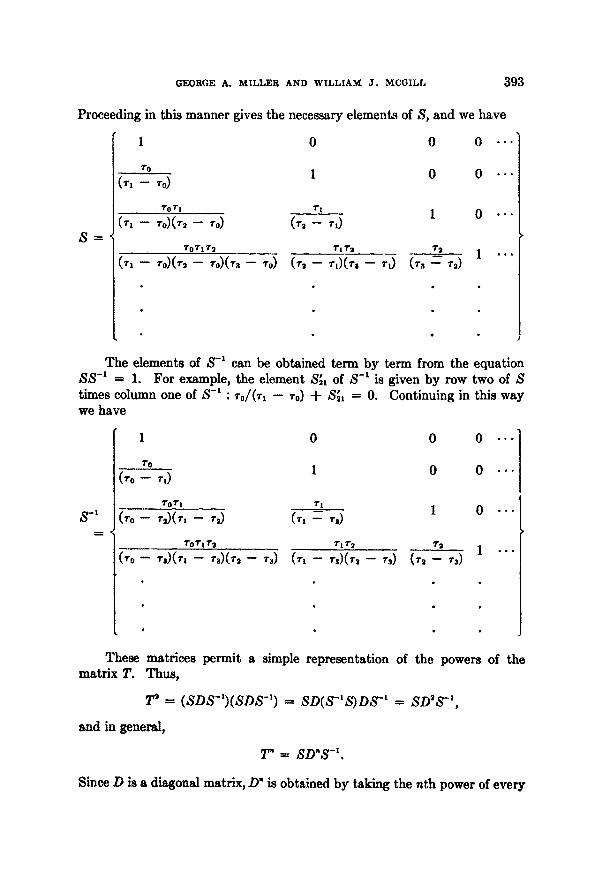
Proceeding in this manner gives the necessary elements of S, and we have

S =

1 0 0 0 ""1

l TO

(rl -- To) 1 0 0 " ' "

TO 1.1 TI

(T~ - To)(T~ - - To) ( T , - T,) 1 o

,,, TOTI T2 ................... 1.1 T2 T2 I ( r , - - To)(rn-- To)Cr,-- To) (1.,-- TI)(T,-- v~ (Ts - -T, ) 1 . . . l

o

The elements of S -~ can be obtained term by term from the equation SS -1 = 1. For example, the element S~ of S -1 is given by row two of ~g times column one of S -s : ro/(rl -- To) -t- Sis = O. we have

Continuing in this way

1To 0 0 0 "'i]

E (To - r,) 1 0 0

TOTI . T1 (To -- r , ) (r , -- T,) (r, -- 1.,1 1 0 . . .

roT! 1.9 TI 1"2 T~ I ° °°

(~1 - ~)(~, - ~) (~, - ,~) (To- 1.~)(~I - ~)(,,- ~)

These matrices permit a simple representation of the powers of the matr ix T. Thus,

T ~ _- ( S D S - I ) ( S D S -~) = S D ( S - I ~ D 5 '-~ = S D ' S -i ,

and in general,

7" = ,gD~S -~.

Since D is a diagonal matrix, D" is obtained by taking the n th power of every

394 PSYCHOMETRIKA

diagonal element.

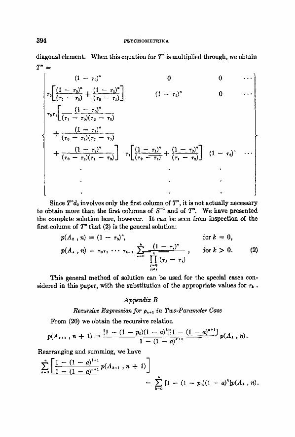
T" =

(I - ~-o)"

- ,o)" --_ , , ) " ] ro ( ,~ _ 'o) + (~-o - , , ) J

~o', [ , / (1 , - 7o)", .... - t * , - ~'o)0",- ~'o)

(1 -- r,)" +

(3 _- "_~)"_ 7 + (~o - ,~) ( , , - ~.,) J

When this equation for ~" is multiplied through, we obtain

0 0

(1 -- ~',)" 0

[ ' (1 - - r , ) " (1 - - r2)" 7 (1 - - r2)" " - "

Since T"do involves only the first column of T", it is not actually necessary to obtain more than the first columns of S -L and of T". We have presented the complete solution here, however. I t can be seen from inspection of the first column of T" that (2) is the general solution:

p(Ao, n) = (1 - to)", for k = 0, t

~ _ _ (1 -- r,)" for k > 0. (2) p(Ak, n) = ror~ . . " rk-, ~ , , - o 1-I (~ , - , , )

i - 0

This general method of solution can be used for the special cases considered in this paper, with the substitution of the appropriate values for r~ .

Appendix B

Recursive Expression for p.+l in Two-Parameter Case

From (20) we obtain the recursive relation

p ( A , ÷ , , n + 1)_= [1 -- (I -- po)(l -- a)*][l -- (1 -- a) "÷ ' ] p ( A , , n). 1 - ( 1 - a - - ~ - + ' -

Rearranging and summing, we have

,-o ~ -1 (1 a),+ , p(A,+, , n + 1)

' ~ [1 - (1 -- po)(1 - a)~]p(Ak, n). 1 . . 0

GEORGE A. MILLER AND WILLIAM J . MCGILL ~ 9 5

The right side of this equation is, from (5) and (18), p.,~ . be rewritten

] 1 -- (1 - - a ) ' ~-i -- ( 1 - - a) " ÷ ~ p ( A ~ ' n + 1) = p . ÷ , ,

which becomes on trial n (with n >__ 1),

, . , ( I p ( A , , ,,) = p . .

We now have, by adding and subtracting p(Ao, n),

1 - - ( 1 - - a ) " , - o P ( A ' ' n ) - ,-o(1 - a ) ~ p ( A , , n ) = p. ,

1 - ~ (1 - a)~p(A~, n) = [1 - (1 - a)"]p. . k-O

:Now we know that

p.+~ -- 1 - (1 - Po) L (1 - a)~p(A,, n), k-O

and so we obtain

p.+, ---- i -- (I -- po){l -- [I -- (I -- a)"]p.}.

Rearranging terms gives

p.+, = po + (1 - po)[1 - (1 -- a)"]p. ,

which is the desired result. From this result (15) is obtained directly by equating Po and a.

The left side can

(21)

a

A~

d. D k m

n

N Nk,n

Po

Appendix C

List of Symbols and Their Meanings

parameter. state that a word is in after being recalled k times. parameter. infinite column vector, having p(Ak, n) as its elements. infinite diagonal matrix similar to T. number of times a word has been recalled. asymptotic value of r~ and p . . number of trial. total number of test words to be learned. number of words in state Ak on trial n. probability of recalling a word in state A~.

396 PSYCHOMETRIKA

p(A. ,n) r . p~

8 t~ tk.m Tk

T Var (r.)

Xiok,n+l

probabili ty tha t a word will be in state Ak on trial n. observed recall score on trial n; estimate of p , . probability of recall on trial n. elements of S. elements of S -~. infinite matr ix used to transform T into a similar diagonal matrix. estimate of rk . observed fraction of words in state A, tha t are recalled on trial n. probabili ty of recalling a word in state A~. infinite matr ix of transition probabilities rk . variance of the estimate of p . . random variable equal to 1 or 0.

REFERENCES

1. Bush, R. R., and Mosteller, Frederick. A linear operator model for learning. (Paper presented to the Institute for Mathematical Statistics, Boston, December 27, 1951.)

2. Cooke, R.G. Infinite n~trices and sequence spaces. London: MacMillan, 1950. 3. Estes, W.K. Toward a statisticzl theory of learning. Paychol. Re~., 1950, 57, 94-107. 4. Feller, W. On the theory of stochastic processes with particular reference to applica-

tions. Proceedings of the Berkeley Symposium on Mathematical Statistics and Probability, 1949, 403-432.

5. Woodbury, M.A. On a probability distribution. Ann. math. Statist., 1949, 20, 311- 313.

Manuscript reccb~ 3/11/58

Documents

A statistical description of verbal learning