! "!

A statistical interpretation of surface ocean temperature trends during the Paleocene-Eocene Thermal Maximum

Nathan M. Urban a,b,*, Timothy J. Bralower a, Murali Haran c, and Klaus Keller a,d a Department of Geosciences, Pennsylvania State University, University Park, PA 16802, USA

b current affiliation: Woodrow Wilson School of Public and International Affairs, Princeton University, Princeton, NJ 08544, USA

c Department of Statistics, Pennsylvania State University, University Park, PA 16802, USA

d Earth and Environmental Systems Institute, Pennsylvania State University, University Park, PA 16802, USA

* Corresponding author. E-mail address: nurban@princeton.edu (N. Urban)

! #!

Abstract

$%&!'()&*+&,&-.*+&,&!/%&01()!1(23141!5'.$67!8)*9()!:(013,8!&;&,/!5+(<!==<=!6>(7!3? often considered a geologic analog to the modern, rapid addition of carbon dioxide to the atmosphere. The ability to assess the sensitivity of many rate-dependent climate change impacts, based on the PETM analogy, hinges critically on the PETM warming rate. Current estimates of the PETM warming rate face considerable problems, for example, due to the nontrivial statistical challenges in accounting for the key known uncertainties in a mathematically sound way.

Here we introduce a new method for quantifying the PETM warming rate recorded by the oxygen isotopes of single-specimen surface-dwelling foraminifera at Southern Ocean ODP Site 690. We use Monte Carlo samples from the Bayesian predictive distribution of reconstructed climate histories to estimate the probability distributions of millennial temperature trends. Our approach produces probabilistically sound hindcasts of the observations and the implied rates of change that comprehensively account for the combined effects of uncertainties in (i) proxy measurement, (ii) age estimates, (iii) long term rates of temperature change, (iv) the autocorrelated natural temperature variability, and (v) the conversion from proxy to temperature. We test the sensitivity of the reconstruction to the choice of chronology by comparing the results derived from two independent chronologies, based on orbital cyclostratigraphy and extraterrestrial helium-3 (3He) accumulation.

We estimate the peak millennial-scale warming rate (at the onset of the PETM) as 1.4 °C/kyr (with a 95% credible interval from -2.3 to 5.4 °C/kyr) using orbital chronology and 1.1 °C/kyr (95% credible interval from -2.5 to 4.9 °C/kyr) using 3He age control. By comparison, a suite of IPCC AR4 AOGCM model projections for the 21st century predict ocean surface warming rates at the Southern Ocean site ranging from -4 to 14 °C/kyr, when extrapolated from century to millennial scale rates, with half of the models projecting rates of less than 3 °C/kyr. Although the paleo-reconstruction method cannot resolve century scale changes, we conclude that Site 690 data support a PETM peak warming rate of a magnitude potentially comparable to (possibly only 2-3 times slower than) the rate of warming projected for the next century. An unresolved caveat is whether the onset of the PETM at Site 690 is truncated due to a brief period of dissolution, leading to a spuriously high apparent rate of warming.

! @!

1. Introduction

The PETM has been analysed extensively and is now cited as one of the best, if not the best, ancient analog for modern global warming [e.g., Zachos et al., 2001]. The PETM had a wide range of impacts on terrestrial and marine biotas, coinciding with the largest mass extinction event in the deep sea in the last 90 Myr (Tjalsma and Lohmann, 1983; Thomas, 1990). Organisms inhabiting the sea surface, including planktonic foraminifera and nannoplankton, underwent a remarkable transient turnover driven by a combination of warming and changing resource availability (e.g., Kelly et al., 1996, 1998; Bralower, 2002; Kelly, 2002; Gibbs et al., 2006; Agnini et al., 2007; Raffi et al., 2009; Bown and Pearson, 2009). Terrestrial plants were characterized by wholesale but transient shifts in distribution as a result of warming and changing precipitation patterns (e.g., Wing et al., 2005); terrestrial faunas also saw significant migration as a result of climate change and the development of land bridges (e.g., Clyde and Gingerich, 1998; Gingerich et al., 2003).

One key open question is, with the exception of deep-sea organisms, why this abrupt event caused so few permanent effects on fauna and flora? Was it because the rates of warming, and, by assumption, the rates of niche replacement, were too sluggish? Or was it because species living at that time were well adapted to a rapid change in their environment?

This investigation explores the first question: what was the rate of warming throughout the PETM? In particular, what was the peak rate of warming and when did it occur? And, importantly, what measures of uncertainty, or what levels of statistical confidence, are attached to these estimates? Previous estimates of rates of carbon cycling and warming during the PETM are based on linear interpolation of data across segments of the event that are anchored by duration estimates (e.g., Zachos et al., 2003; Panchuk et al., 2008; Zeebe et al., 2009; Ridgwell and Schmidt, 2010; Cui et al., 2011). The most widely cited estimates for the total warming are model based (e.g. Sloan and Thomas, 1998), and do not lend themselves for dissecting the various stages of the event.

Although questions about PETM warming rates are simply posed, answering them presents nontrivial methodological challenges. Rate estimates must account for sources of error in both the reconstructed temperatures and in the chronology, and these errors may be correlated across time and space. The data themselves are irregularly and sometimes sparsely sampled in time, and may record relatively abrupt environmental changes, confounding simple sliding window or smoothing approaches to derivative estimation.

! A!

Here we provide temperature rate estimates and comprehensive error analysis of the oxygen-18 (

!

" 18O) temperature proxy during the PETM, recorded in single-specimen surface dwelling planktonic foraminifera sampled from a single ocean core, Southern Ocean Ocean Drilling Program (ODP) Site 690 (Thomas et al., 2002). The oxygen isotope (!18O) temperature proxy data (Figure 1) are a classic depiction of the PETM event: an abrupt, negative oxygen isotope shift coincident with a large negative carbon-13 (

!

" 13O) isotope excursion (CIE), consistent with global warming resulting from a large input of greenhouse gases to the atmosphere (e.g., Kennett and Stott, 1991; Dickens et al., 1995; Bains et al., 1999; Panchuk et al., 2008; Zachos et al., 2008). Single specimen data capture the range of environmental variability in the habitat of the surface-dwelling foraminifera; multi-specimen analyses (e.g., Kennett and Stott, 1991) fail to capture this variability. However, single specimen analyses are more prone to the effect of sediment mixing by bioturbation. Fortunately the magnitude of the CIE provides a means whereby reworked specimens can be identified (e.g., Kelly et al., 1996). With the exception of a few specimens near 171 mbsf, there appears to be little reworking across the CIE at Site 690.

FIGURE 1: Oxygen (left) and carbon (right) isotope measurements from the Site 690 core, extracted from single surface-dwelling foraminiferal specimens, as a function of depth (in meters below sea floor, mbsf) (replotted from Thomas et al.,

! =!

2002). The lower dashed line (“event”) indicates the location of the negative carbon isotope excursion (PETM event) visible in the right panel, coincident with an abrupt warming (negative oxygen isotope shift) visible in the left panel. The upper dashed line (“?”) indicates a second apparent abrupt warming, following the PETM, which appears coincident with a positive carbon isotope excursion.

The samples are dated using two independent chronologies, giving two separate rate estimates. Although a single-core analysis neglects the (possibly dominant) uncertainty introduced by differing and possibly conflicting core chronologies, this simplification is partially ameliorated by the use of independent chronologies. The approach is a methodological advance on rate estimation for individual cores, and is applicable to the data from any core, thus paving the way for future multi-site analyses.

Our new methods are based on a “climate history” approach, wherein many hypothetical temperature time series consistent with the proxy data are reconstructed by a Monte Carlo sampling procedure. The probability distribution assigned to these time series is obtained from a Bayesian inferential approach that learns from the proxy data while accounting for uncertainties appropriately. An advantage of the climate history sampling method is that once the histories are generated, all statistical questions reduce to simple counting. For example, if one wants to know the probability that the rate of temperature change exceeded a particular value at a particular time, it suffices to merely count the fraction of the temperature histories in the sample that exceed the rate in question.

The climate history method accounts for uncertainties in rate due to a variety of possible error sources. We consider errors due to measurement error in temperature proxies, along with other unattributed sources of error in the proxy data, and uncertainty in the proxy-temperature relationship. The proxy errors may be correlated in time, with an unknown correlation time scale estimated from the data. The underlying long-term trend may undergo abrupt changes; the changepoints are estimated from the data as well. In addition to an overall sensitivity analysis to the type of chronology used, the statistical method also accounts for errors in the ages of individual proxy samples.

2. Chronology

Given the importance of understanding the causes and consequences of the PETM, especially as they compare to modern climate change, there has been considerable attention paid to estimating the detailed chronology of the event. Two fundamentally independent approaches have been applied to determine the duration of various stages of the event as defined by the carbon isotope excursion, including the onset (the point where !13C values begin to decrease), the peak (the interval corresponding to the lowest !13C

! B!

values), and the recovery (the interval where !13C values increase towards pre-PETM values). The first technique applies orbital stratigraphy (e.g., Norris and CD%), 1999; CD%) et al., 2000; CD%) et al., 2007; Charles et al., 2011). This technique is based on counting the number of orbital cycles in continuous time series (usually elemental data) from the PETM interval and constraining the periodicity of these cycles (using time series analysis). The major uncertainties associated with this method derive from determining the exact number of cycles where these variations are equivocal, and, more problematic, from “burn down” (e.g., Walker and Kasting, 1992) that has removed existing sediment at the base of the event in several sections via an interval of intense dissolution (e.g., Zachos et al., 2005). Also, identification of the termination of the event can be quite subjective due to the asymptotic shape of the !13C curve in the recovery interval.

The alternate dating technique is based on measurement of helium-3 (3He), an isotope that is almost entirely derived from extraterrestrial sources. A small amount of 3He is terrestrial in origin, but this source has very different 3He/4He ratios from extraterrestial helium and can be readily identified. Extraterrestrial 3He is assumed to accumulate at the Earth’s surface at a constant rate (e.g., Ozima et al., 1984) and its concentration is thus a function of the amount of dilution by sediment (i.e. a measure of sedimentation rate). This technique is dependent on determining the sediment accumulation rate of some interval in the section. In the case of the PETM, the accumulation rate is estimated from the duration of Chron C24R (e.g., Farley and Eltgroth, 2003). 3He chronology is affected in a different way as a result of burn down than is orbital chronology. Removal of section at the base of the event will not alter the total duration of the interval studied; however, “burn down” will shift the position of the base of the event to a lower stage in the relative 3He chronology (see below).

We analyze data from ODP Site 690, a location that is generally recognized to have more continuous deposition at the base of the PETM than other deep-sea sections. Site 690 was shallow enough that it remained above or within the lysocline for the entire event, whereas most other deep-sea sites lay below the CCD for a short time at the onset of the event (Kelly et al., 2005; Colosimo et al., 2005; Zachos et al., 2005), so chronologies based on this section are likely to be more precise than other deep sea sites. Moreover, the occurrence of precessional cycles at Site 690 demonstrates that sedimentation rates are higher than in other deep-sea locations where only eccentricity cycles can be identified (e.g., Shatsky Rise, ODP Leg 198; Westerhold et al., 2008). The PETM corresponds to 11 precessional cycles at Site 690 (Rohl et al., 2007) with 5 cycles corresponding to the onset and peak (~100 kyr) and 3.5 cycles (~70 kyr) within the

! E!

recovery. The latter number is a little uncertain given that the top of the !13C excursion lies in a coring gap. By comparison at Forada, a hemipelagic section from the Southern Alps of Italy, there are 11 precessional cycles within the PETM with 5 cycles in the onset and peak (100 kyr) and 6 cycles within the recovery (120 kyr; Giusberti et al., 2007).

Using 3He isotope measurements, Farley and Eltgroth (2003) constrained the onset and peak of the PETM at Site 690 to 80 kyr and the recovery to 30 kyr. This estimate of the recovery is much shorter than estimates using cyclostratigraphy, however, the duration of the onset and peak are relatively similar for Site 690 and the Forada section based on cyclostratigraphy (Giusberti et al., 2007; Rohl et al., 2007) and 3He (Farley and Eltgroth, 2003). In a recent investigation by Murphy et al. (2010), 3He measurements at Site 1263 indicated much longer durations for every stage of the PETM, most significantly the onset of the event (35 kyr). Burn down at this site likely lowered the CIE below its true stratigraphic position, artificially lengthening the duration of the onset of the PETM (B. Murphy, pers. comm., 2011).

The base of the PETM at Site 690 is sharp and the onset of the CIE corresponds to just three cm of sediment (Thomas et al., 2002). This amount is well within one precessional cycle. Although increased dissolution at the base of the event is likely, two pieces on information render it unlikely that such dissolution progressed far enough to cause “burn down”: carbonate content remains above 60% throughout the event, and a sequence of isotopic and biotic changes is preserved in the interval 10-20 cm below the CIE (Thomas et al. 2002; Bralower et al., 2002; Kelly et al., 2002). Burn down would presumably result in an interval without carbonate and would tend to focus the isotopic and biotic change. Since burn down has different effects on orbital and 3He age models, it can also theoretically be identified by comparing the two age models.

Figure 2 explores the consistency between the orbital and helium dating methods. The left panel shows all age data available for Site 690 as a function of depth, including periods of time for which no foraminiferal specimens are available (i.e., outside the range of depths depicted in Figure 1 and analyzed in this study). The right panel shows a plot of helium age vs. orbital age for the period of time depicted in Figure 1. One way burn down could manifest itself is in a cusp or discontinuity in these curves. For example, if some section is missing due to burn down, causing the cyclostratigraphic method to miss a cycle, this could manifest as a sudden apparent jump in helium age relative to orbital age (as the extraterrestrial helium continues to accumulate). No such features are visible in Figure 2. This does not prove that imperceptibly small intervals of the core are missing, but does provide some confidence in validity of the chronologies.

! F!

FIGURE 2: Comparison of orbital and helium chronologies. Left: orbital and helium ages plotted as a function of core depth below sea floor. The shaded region indicates the range of ages considered in the present study. The dashed lines are the features (CIE “event”, and a unknown possible event “?”) indicated in Figure 1. Right: scatterplot of helium vs. orbital ages.

3. Methods

We next outline the general method in conceptual terms, and discuss key assumptions, motivation, and interpretation. A fully mathematical treatment of the statistical methods, and the parameter estimates which result, is contained in the Supplementary Material.

The combined temperature reconstruction and error analysis is based on the statistical technique of Bayesian Gaussian process regression [see Rasmussen and Williams (2006) for a review], which is used in combination with Monte Carlo simulation to reconstruct a large sample of possible “climate histories”. The imputed climate histories are regularly spaced in time, permitting the application of simple sliding-window linear derivative estimates to determine rates over time. The imputation process incorporates uncertainty into the analysis by matching the variability in the reconstructed climate histories to the variability present in the core data. The uncertainty in the temperature rate is given by the spread of rates found in the collection of climate histories.

The four-part statistical method is summarized in Figure 3.

! G!

FIGURE 3: Schematic depiction of the statistical temperature reconstruction method; each panel corresponds to a step discussed in Section 3. Ages are determined by orbital chronology.

Step 1.

In the first step, a piecewise linear regression is fit to the

!

" 18O temperature proxy data. The linear model is constructed to have three periods of gradual linear temperature change, divided by two periods of rapid change. This structure reflects two changepoints that are apparent in the proxy data. The earlier changepoint corresponds to the PETM event, and is coincident with the negative carbon isotope excursion (Figure 1). The later changepoint corresponds to further warming apparent in the Site 690 data, ~30-60 kyr after the original event (depending on chronology). In addition to the linear slopes and intercept coefficients, the regression also estimates the changepoint locations, although

! "H!

they are constrained by their prior distributions to lie within 5 kyr of their apparent ages. Four changepoint locations are estimated, with a pair of changepoints immediately preceding and following each of the two periods of abrupt temperature change.

The error process in the linear regression model is the sum of an independent and identically distributed (iid) normal error process and a temporally autocorrelated normal error process, decaying exponentially with time. The former represents measurement and other unresolved proxy errors, while the latter represents correlated natural variability in climate. The iid and correlated error variances and the correlation timescale are estimated along with the regression coefficients and changepoints.

The Bayesian parameter estimation procedure assigns a full joint probability density function to the unknown parameters, not simply point estimates or confidence intervals. The Metropolis Markov chain Monte Carlo (MCMC) algorithm is used to sample from the joint posterior probability distribution of the unknown parameters. The resulting sample represents candidate hypotheses for the possible values of the parameters, with more probable values appearing more frequently in the sample. The set of parameters, in turn, generates many candidates for piecewise linear fits to the data. The first panel in Figure 3 shows the mean (solid line) and 95% predictive envelope (dashed lines) for the posterior sample of linear fits.

Step 2.

The fits in the first step of the reconstruction method are all piecewise linear. The second step uses Gaussian process regression to condition each sample reconstruction on the measured data. This allows the fits to adapt locally to the data in a nonlinear manner. Figure 3 (second panel) shows the resulting mean and predictive envelope for the sample of conditional reconstructions.

Step 3.

The third reconstruction step samples random “proxy histories” from the predictive envelope computed in the second step. This amounts to superimposing random noise realizations from the iid and correlated error processes onto the fits from the second step. This serves to interpolate the proxy data onto a regular temporal grid. Each proxy history is a candidate for what the measured

!

" 18O would be at a series of evenly spaced points in time, if foraminiferal specimens from those dates existed in the core sample, accounting for natural climate variability and proxy measurement error. The histories vary in terms of their generating parameters sampled in the first step, so that each history may have a different underlying piecewise linear mean function, set of changepoint locations, and

! ""!

error variance and autocorrelation. A sample proxy history is shown in Figure 3 (third panel).

Step 4.

The fourth reconstruction step converts the proxy histories to temperature histories. The usual proxy conversion procedure fits a regression of temperature vs. proxy to a set of calibration measurements of laboratory-grown foraminifera (Erez & Luz, 1983). The proxy data and fit are given in Supplemental Figure 3. The regression is used to predict a new temperature given a new proxy measurement. This common procedure is, however, statistically problematic. A regression of temperature on proxy treats temperature as the dependent variable and proxy as the independent variable. However, in the experimental calibration data, temperature is the controlled variable, and proxy is the measured variable. Reversing the distinction between dependent and independent variables, while convenient, violates the statistical assumptions of the regression. This can produce regression estimates that are biased (Durbin, 1954) — a phenomenon sometimes known as “regression dilution” — as well as incorrect uncertainty intervals

Although we have not assessed the importance of these potential problems to inferring temperatures from proxy data, we opt to apply a more formally correct statistical procedure known as “calibration” or “errors in variables” regression [see Osborne (1991) for a review]. This calibration method treats temperature as the controlled variable and the proxy as the response variable, but allows for errors to exist in the control variable, instead of in the response variable as in ordinary regression.

Bayesian errors-in-variables calibration produces a probability distribution for the predicted temperature corresponding to a proxy measurement. The final reconstruction step, in Figure 3 (fourth panel), samples a random temperature from this distribution for each hypothetical proxy measurement to turn a proxy history into a temperature history. Each temperature history represents a hypothesis for what the temperature would be at each time, were such a measurement possible, accounting for the error in measurement (including the proxy-temperature conversion). It is important to note that the resulting temperature histories represent hypothetical temperature measurements, including measurement error, and not the underlying “true” temperatures. The inclusion of temperature error increases the uncertainty about warming rates beyond the rate that would be calculated if only the most likely temperature for each proxy value were assumed.

Short term trends.

! "#!

The end result of the reconstruction process is a sample of temperature histories interpolated onto a regular grid. Because the imputed temperatures are evenly spaced in time, ordinary least squares estimates of short-term temperature trends can be consistently applied to provide temperature rate estimates over any desired time window. Our approach uses samples from the Bayesian predictive temperature distribution to generate the replicates, which in turn is used to produce a sample-based quantification of the uncertainty in the short-term temperature rates at any given time. This Monte Carlo method may be thought of as the Bayesian analogue of a parametric bootstrap (see, e.g., Efron and Tibshirani, 1994). A sliding 21-point window of width 1 kyr is passed over each temperature history to compute the short-term temperature rates over time. (The trend indicated in Figure 3 is for a >6 kyr window, exaggerated for visual clarity.) When applied to the entire sample of temperature histories, the resulting sliding window estimates constitute a posterior probability distribution for the short-term temperature rates at any given time.

Age uncertainty.

Age uncertainty has been ignored thus far in this discussion. To account for dating errors, error-in-variables regression is applied in the first step. This simultaneously accounts for errors in both the proxy values and the proxy dates. In addition to the regression parameters estimated in the first step, the errors-in-variables regression estimates a set of latent “true ages” corresponding to each of the measured ages from the core chronology. It is assumed that foraminiferal specimens at the same depth share the same latent age. Sediment bioturbation likely violates this assumption, but the assumption renders the regression more computationally tractable by reducing the number of unknown parameters to estimate. The resulting latent age estimates are used in all of the subsequent steps to produce the proxy and climate histories: when generating a history, the proxy data are assumed to be located at their estimated latent ages, rather than their measured ages. The errors-in-variables regression for the latent ages imposes an ordering constraint, so that specimens deposited higher in the core must have younger ages than deeper specimens.

4. Results and Discussion: PETM temperature reconstruction

4.1 General findings.

The distribution of reconstructed temperature histories is shown in Figure 4 for the two chronologies, with the proxy data (converted to temperature) overlaid. The figure can be

! "@!

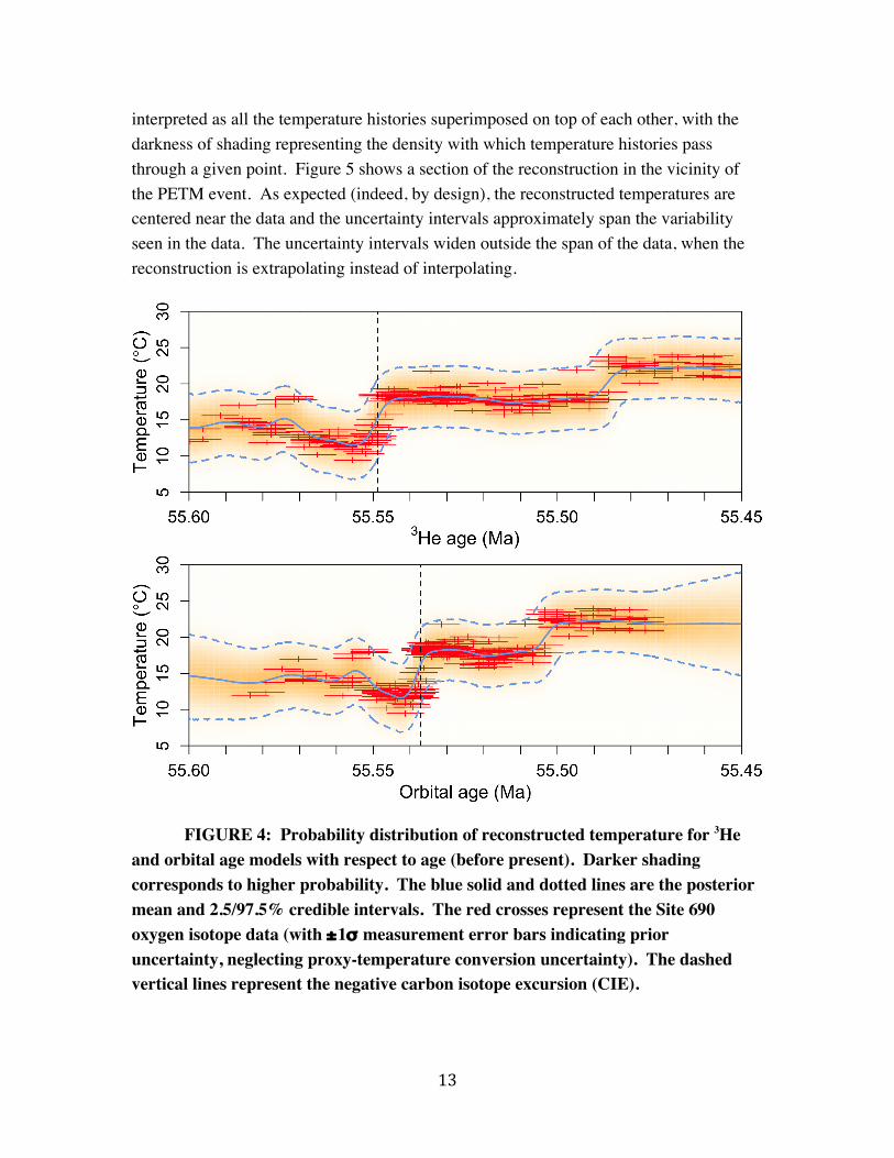
interpreted as all the temperature histories superimposed on top of each other, with the darkness of shading representing the density with which temperature histories pass through a given point. Figure 5 shows a section of the reconstruction in the vicinity of the PETM event. As expected (indeed, by design), the reconstructed temperatures are centered near the data and the uncertainty intervals approximately span the variability seen in the data. The uncertainty intervals widen outside the span of the data, when the reconstruction is extrapolating instead of interpolating.

FIGURE 4: Probability distribution of reconstructed temperature for 3He and orbital age models with respect to age (before present). Darker shading corresponds to higher probability. The blue solid and dotted lines are the posterior mean and 2.5/97.5% credible intervals. The red crosses represent the Site 690 oxygen isotope data (with ±1" measurement error bars indicating prior uncertainty, neglecting proxy-temperature conversion uncertainty). The dashed vertical lines represent the negative carbon isotope excursion (CIE).

! "A!

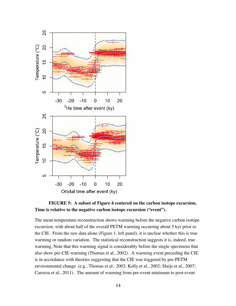
FIGURE 5: A subset of Figure 4 centered on the carbon isotope excursion. Time is relative to the negative carbon isotope excursion (“event”).

The mean temperature reconstruction shows warming before the negative carbon isotope excursion, with about half of the overall PETM warming occurring about 5 kyr prior to the CIE. From the raw data alone (Figure 1, left panel), it is unclear whether this is true warming or random variation. The statistical reconstruction suggests it is, indeed, true warming. Note that this warming signal is considerably before the single specimens that also show pre-CIE warming (Thomas et al., 2002). A warming event preceding the CIE is in accordance with theories suggesting that the CIE was triggered by pre-PETM environmental change (e.g., Thomas et al., 2002; Kelly et al., 2002; Sluijs et al., 2007; Carozza et al., 2011). The amount of warming from pre-event minimum to post-event

! "=!

maximum is 6.6 ± 3.2 °C (

!

1" errors), consistent with the 5.8 °C found by the independent Mg/Ca temperature proxy at Maud Rise Site 690B (Schmidt et al., 2008).

A puzzling feature of the data, visible but not discussed in Thomas et al. (2002), is a second period of warming recorded in the surface-dwelling foraminifera (indicated by “?” in Figure 1). This warming coincides with a positive shift in carbon isotopes (Figure 1, right panel), suggesting a drawdown of atmospheric carbon during the recovery from the initial PETM event. It is unclear why a second period of warming exists, nor why warming would be associated with a decrease in atmospheric carbon. Although this study only studies the surface foraminiferal data from Site 690, the data in Thomas et al. (2002) do not show a corresponding change in !13C or !18O in the thermocline-dwelling planktonic specimens. The thermocline data in Thomas et al. (2002) do indicate a second period of warming, but is smaller and occurs later than the second period of warming in the surface specimens. The thermocline warming is also somewhat inconsistently recorded, with roughly half the specimens showing no warming.

4.2 Uncertainty intervals.

The uncertainty intervals (95% Bayesian credible intervals) in the reconstruction (Figure 3) appear too wide at times after the PETM event, comfortably enclosing all of the data instead of 95% of it. This is likely a consequence of assuming a stationary covariance distribution for the error process, i.e., that the errors are of the same size at all times. The data suggest a possible brief warming excursion about 15–25 kyr before the event, depending on age model (most visible in Figure 5, or in Figure 1 at 171.03–171.14 mbsf). These “outliers” (not to be confused with the smooth pre-PETM warming, ~5 kyr before the onset, discussed in the previous section) inflate the estimated overall variance of the time series, which is propagated to a wider uncertainty interval everywhere in the reconstruction. Conceivably these outliers do not represent a true climate change, but result instead from bioturbation of specimens from the PETM event downward in the sediment column. However, it is difficult to see how bioturbation could mix specimens so far without evidence of mixing at later times before the event.

In our analysis we choose to treat the outlier data as a real climate event and incorporate it into the analysis, rather than discarding it. This is a conservative choice, insofar as it may tend to inflate the estimated natural climatic variability and therefore the uncertainty in short term rates. If the data represent a real climate event, this variation can be handled statistically in two different ways. One is to treat the variability in the data as constant in time. Under this stationarity assumption, the pre-PETM “outliers” may imply a large uncertainty in temperature at later times (such as at the onset of the event), on the

! "B!

grounds that such temperature excursions may repeat themselves later even if not clearly reflected in the data. The second approach is to treat natural variability as non-stationary (changing with time), so that variation in early times may not imply similar variation at later times. Statistics alone cannot determine which approach is more appropriate, as the nature of climatic variability involves scientific judgement. We choose to use the stationary variance assumption, but briefly discuss the merits of some alternate approaches, using hierarchical modeling, in the Supplementary Material.

4.3 Effects of age uncertainty.

Assumptions about age uncertainty affect the reconstructions (Figures 4 and 5). The reconstructions in Figures 4 and 5 include this age uncertainty, examining the sensitivity to the chronology used. Orbital dating, in general, favors a more rapid warming event and an overall shorter duration of time spanning the core data. This could be due to a combination of a short pulse of dissolution at the onset of the CIE combined, possibly with sediment burndown. However, within a given chronology, it is also informative to explore the sensitivity of the reconstruction to whether individual dates themselves are considered to be uncertain. This sensitivity analysis is shown in Figure 6 using the orbital chronology, comparing the reconstruction with age uncertainty to an alternate reconstruction in which the measured ages of the specimens are assumed to be their true ages, without error. The sensitivity analysis indicates that when errors in individual age estimates are allowed, the temperature reconstruction is smoothed in time, reducing the estimated PETM warming rate. The estimated latent ages and their uncertainties are shown in Supplemental Figure 4.

! "E!

FIGURE 6: Posterior mean temperature reconstruction including (solid line) and excluding (dashed line) uncertainty in individual ages, both using orbital dating. Gray crosses are the Site 690 data with an assumed 0.08‰ prior proxy uncertainty (neglecting proxy-temperature uncertainty) and 5 kyr prior age uncertainty.

5. Results and Discussion: PETM and modern warming rates

A simple calculation of the maximum PETM warming rate can be made from the step 1 linear regression slope estimate for the first abrupt period (coincident with the onset of the PETM and the CIE). The marginal posterior distribution of this parameter has a mean of -579 ‰/Myr (-2131 to -122 ‰, 95% ci) for orbital dating or -670 ‰/Myr (-1590 to -106 ‰, 95% ci) for helium dating (see Supplemental Figures 1 and 2 for the probability distributions of this parameter, labeled mtrans1). Assuming a conversion factor of 4.52 °C/‰ (see SI), the corresponding temperature rates are 2.6 (-0.6 to 9.6, 95% ci) °C/kyr for orbital dating and 2.0 (-0.5 to 7.2, 95% ci) °C/kyr for helium dating. The similarity of the rate estimates based on orbital and 3He chronology suggest to us that dissolution and sediment burndown at Site 690 are both minimal.

Warming rate estimates depend on estimates of both the amount and duration of the warming interval. Although we have focused on how biases in chronology may affect the estimated warming rates, it is also worth considering whether the oxygen temperature proxy accurately reflects the magnitude of warming. Biases can occur, for example, if

! "F!

the ocean salinity varies throughout the event. As an independent check, we consider the Mg/Ca temperature proxy, which implies a ~5.8 °C warming across the event (Schmidt et al., 2008). This comparable to the ~6.6 °C warming found in this study (Figure 5), corresponding to an additional ~10-15% uncertainty in warming rates due to choice of temperature proxy. This source of uncertainty is omitted from subsequent analysis, but should be borne in mind.

The simplified warming rate calculation reduces the onset warming to a linear trend, and the uncertainties reported are errors in the linear trend, not in the actual reconstructed temperature time series, which is noisy and nonlinear. A linear trend estimate captures the average rate over the duration of the event, but is less suited to estimating the peak (maximum) rate of warming. The full “climate history” approach is able to give a more nuanced, and time-dependent picture of how temperature rates evolved over time. Henceforth we consider the climate history approach to estimating the peak warming rate during the PETM event.

The peak PETM temperature rate distribution is calculated by first finding the time at which the mean short-term (1 kyr) rate, averaged over all the temperature histories, achieves its maximum value. Then a histogram is constructed of the short-term temperature rate, calculated at that time, for each temperature history. This distribution is estimated for both chronologies (orbital and helium).

The peak PETM rate distributions (and mean and 95% Bayesian credible intervals) are displayed in Figure 7. The mean peak PETM millennial-scale warming rate is estimated to be 1.4 °C/kyr, with a 95% Bayesian credible interval of -2.3 to 5.4 °C/kyr, using orbital chronology. The mean peak rate is slightly lower when using helium dating, 1.1 °C/kyr, with a 95% interval of -2.5 to 4.9 °C/kyr. These rate estimates are lower than the prediction of the simple regression slope calculation presented earlier.

Interestingly, the climate history uncertainty intervals for the peak warming rate are narrower than the uncertainty intervals computed using the linear slope method. One might expect them to be wider, since the climate histories contain natural temperature variability about the overall linear trend, and include uncertainty in conversion from proxy to temperature. These uncertainties are not considered by the linear slope approximation. However, the climate histories also condition on the observed proxy data, so that the histories are forced to conform more closely to abrupt transitions in the data that may be averaged over by a linear regression, thus leading to sharper estimates. Also, the regression slope distribution is highly skewed due to an inability to exclude effectively infinite rates with all warming occurring in an arbitrarily short time between

! "G!

data points (see Supplemental Figures 1 and 2). In the climate history approach, the long correlation time of the natural temperature variability may preclude instantaneous warming from occurring in the sample paths even when it occurs in the underlying linear trend, excluding some of the high upper tail of the warming rate.

FIGURE 7: Posterior probability distributions for the peak PETM warming rate using orbital (“O”) and helium (“H”) dating. The mean and 95% credible intervals are reported below the curves as circles and lines, respectively. Above the curves are the mean and 95% confidence intervals for the 21st century warming rates projected by 12 AOGCMs. The numbers refer to the GCMs in the legend of Figure 8.

Nevertheless, the peak PETM warming rate uncertainty intervals arising from the climate history method are quite wide: they are several times larger than the mean trends themselves, and cannot exclude the possibility of short-term cooling. This might be expected from the great uncertainty in reconstructing temperatures over short time scales from limited data. As such, any comparison of PETM warming rates to modern rates should be made with caution. We proceed, noting that we are comparing millennial-scale

! #H!

PETM warming rates to centennial-scale future warming projections. This should not be taken to imply that 21st century warming rates will be sustained over the next millennium.

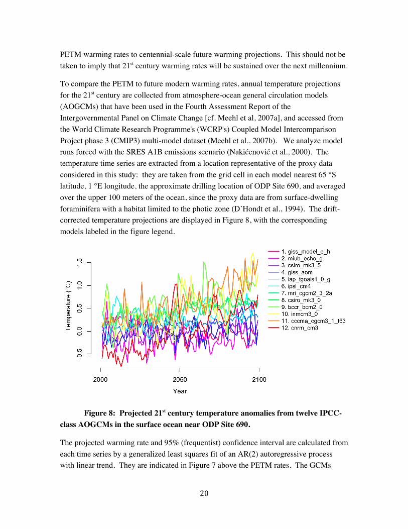
To compare the PETM to future modern warming rates, annual temperature projections for the 21st century are collected from atmosphere-ocean general circulation models (AOGCMs) that have been used in the Fourth Assessment Report of the Intergovernmental Panel on Climate Change [cf. Meehl et al, 2007a], and accessed from the World Climate Research Programme's (WCRP's) Coupled Model Intercomparison Project phase 3 (CMIP3) multi-model dataset (Meehl et al., 2007b). We analyze model runs forced with the SRES A1B emissions scenario (Naki!enovi! et al., 2000). The temperature time series are extracted from a location representative of the proxy data considered in this study: they are taken from the grid cell in each model nearest 65 °S latitude, 1 °E longitude, the approximate drilling location of ODP Site 690, and averaged over the upper 100 meters of the ocean, since the proxy data are from surface-dwelling foraminifera with a habitat limited to the photic zone (D’Hondt et al., 1994). The drift-corrected temperature projections are displayed in Figure 8, with the corresponding models labeled in the figure legend.

Figure 8: Projected 21st century temperature anomalies from twelve IPCC-class AOGCMs in the surface ocean near ODP Site 690.

The projected warming rate and 95% (frequentist) confidence interval are calculated from each time series by a generalized least squares fit of an AR(2) autoregressive process with linear trend. They are indicated in Figure 7 above the PETM rates. The GCMs

! #"!

project rates from -4 °C/kyr (-0.4 °C/century), actually a cooling, to 14 °C/kyr (1.4 °C/century). The average rate over all model projections is 5.0 °C/kyr and half of the model projections rates are less than 3 °C/kyr, compared to the mean peak rates of 1.1 or 1.4 °C/kyr found during the PETM (with helium or orbital dating, respectively). Thus, to the extent that PETM and modern warming rates can be compared by this method, the PETM warming indicated by the Site 690 data is within a factor of 2 or 3 of the rates predicted projected by a number of the GCMs considered, about 4 times slower than the mean GCM projected rate, and is no more than 10 times slower than the highest GCM rate considered here.

The Site 690 chronologies applied here suggest a substantially briefer PETM onset than a detailed new chronology derived from an expanded core from Spitsbergen (Charles et al., 2011; Cui et al., 2011). This core indicates an onset duration of ~19 kyr, more than double the onset at Site 690. As we have discussed, the Site 690 core could be truncated by dissolution and possibly further condensed by burndown, implying a shorter event duration and thus an upwardly biased rate of warming.

6. Conclusions

Was the warming rate during the Paleocene-Eocene Thermal Maximum comparable to projected future rates? We have developed a statistical method to reconstruct rates of temperature change during the PETM. The method accounts for uncertainties in proxy measurement, natural climate variation, age, and the proxy-temperature relationship.

We find a best estimate of the peak surface ocean warming rate during the PETM at ODP Site 690 to be 1.1 or 1.4 °C/kyr, depending on the chronology used (helium and orbital dating, respectively). There is, however, a wide statistical uncertainty about this rate, ranging from -2.5 to +5.4 °C/kyr. The PETM warming rates are within the range of twelve IPCC-class climate model projections, which estimate a 21st century warming rate of -4 to 14 °C/kyr when extrapolated from century to millenial scale rates. Half the models showing a warming of less than 3 °C/kyr, comparable in magnitude to the PETM peak warming rate. We conclude that the Site 690 data support, but do not demonstrate, a warming rate comparable to likely future climate change.

The comparison of paleo and modern warming rates should be viewed cautiously. Future global warming will likely transpire over the course of a few centuries, and the proxy data considered here do not have the power to fully resolve peak paleo warming rates on century time scales. A more complete comparison will require application of the technique described in different locations combined with continuing investigations of the chronology of the onset of the PETM.

! ##!

7. Acknowledgments

We thank Rob Fuller for help with extracting the AOGCM output from the PCMDI archive. Helpful discussions with Lee Kump, Ying Cui, Brandon Murphy, and John Haslett are gratefully acknowledged. We acknowledge the modeling groups, the Program for Climate Model Diagnosis and Intercomparison (PCMDI) and the WCRP's Working Group on Coupled Modelling (WGCM) for their roles in making available the WCRP CMIP3 multi-model dataset. Support of this dataset is provided by the Office of Science, U.S. Department of Energy. This study was partially supported by the Penn State Center for Climate Risk Management. All errors and opinions are (unless cited) ours.

! #@!

References

Agnini, C., Fornaciari, E., Raffi, I., Rio, D., Röhl, U. and Westerhold, T., 2007. High-resolution nannofossil biochronology of middle Paleocene to early Eocene at ODP Site 1262: Implications for calcareous nannoplankton evolution. Marine Micropaleontology 64, 215-248.

Bains, S., Corfield, R.M., Norris, R.D., 1999. Mechanisms of climate warming at the end of the Paleocene. Science 285, 724-727.

Bown, P., Pearson, P., 2009. Calcareous plankton evolution and the Paleocene/Eocene thermal maximum event: New evidence from Tanzania. Marine Micropaleontology 71, 60-70.

Bralower, T.J., 2002. Evidence for surface water oligotrophy during the Paleocene-Eocene Thermal Maximum: Nannofossil assemblage data from Ocean Drilling Program Site 690, Maud Rise, Weddell Sea. Paleoceanography 17, 1023.

Carozza, D.A., Mysak, L.A., Schmidt, G.A., 2011. Methane and environmental change during the Paleocene-Eocene thermal maximum (PETM): Modeling the PETM onset as a two-stage event. Geophysical Research Letters 38, L05702.

Charles, A.J., Condon, D.J., Harding, I.C., Pälike, H., Marshall, J.E.A., Cui, Y., Kump, L., Croudace, I.W., 2011. Constraints on the numerical age of the Paleocene-Eocene boundary. Geochemistry, Geophysics, Geosystems 12, Q0AA17.

Clyde, W.C., Gingerich, P.D., 1998. Mammalian community response to the Latest Paleocene Thermal Maximum: an isotaphonomic study in the northern Bighorn Basin, Wyoming. Geology 26, 1011-1014.

Colosimo, A.B., Bralower, T.J., Zachos, J.C., 2005. Evidence for lysocline shoaling and methane hydrate dissociation at the Paleocene-Eocene thermal maximum on Shatsky Rise. Proceedings of the Ocean Drilling Program, Scientific Results 198, 1-36.

Cui, Y., Kump, L.R., Ridgwell, A.J., Charles, A.J., Junium, C.K., Diefendorf, A.F., Freeman, K.H., Urban, N.M., Harding, I.C., 2011. Slow release of fossil carbon during the Palaeocene-Eocene Thermal Maximum. Nature Geoscience, in press.

D’Hondt, S., Zachos, J.C., Schultz, G., 1994. Stable isotopic signals and photosymbiosis in Late Paleocene planktic foraminifera. Paleobiology 20, 391-406.

! #A!

Dickens, G.R., O’Neill, J.R., Rea, D.K., Owen, R.M., 1995. Dissociation of oceanic methane hydrate as a cause of the carbon isotope excursion at the end of the Paleocene. Paleoceanography 10, 965-971.

Durbin, J., 1954. Errors in variables. Revue de l'Institut International de Statistique / Review of the International Statistical Institute 22, 23-32.

Efron, B., Tibshirani, R., 1994. An Introduction to the Bootstrap. Chapman & Hall/CRC.

Erez, J., Luz, B., 1983. Experimental paleotemperature equation for planktonic foraminifera. Geochimica et Cosmochimica Acta 47, 1025-1031.

Farley, K.A., Eltgroth, S.F., 2003. An alternative age model for the Paleocene-Eocene thermal maximum using extraterrestrial 3He. Earth and Planetary Science Letters 208, 135-148.

Gibbs, S.J., Bralower, T.J., Bown, P.R., Zachos, J.C., Bybell, L.M., 2006. Shelf and open-ocean calcareous phytoplankton assemblages across the Paleocene-Eocene Thermal Maximum: Implications for global productivity gradients. Geology 34, 233-236.

Gingerich, P.D., 2003. Mammalian responses to climate change at the Paleocene-Eocene boundary: Polecat Bench record in the northern Bighorn Basin, Wyoming. Geological Society of America Special Paper 369, 463-478.

Giusberti, L., Rio, D., Agnini, C., Backman, J., Fornaciari, E., Tateo, F., Oddone, M., 2007. Mode and tempo of the Paleocene-Eocene thermal maximum in an expanded section from the Venetian pre-Alps. Geological Society of American Bulletin 119, 391-412.

Kelly, D.C., Bralower, T.J., Zachos, J.C., Silva, I.P., Thomas, E., 1996. Rapid diversification of planktonic foraminifera in the tropical Pacific (ODP Site 865) during the late Paleocene thermal maximum. Geology 24, 423-426.

Kelly, D.C., Bralower, T.J., Zachos, J.C., 1998. Evolutionary consequences of the latest Paleocene thermal maximum for tropical planktonic foraminifera. Palaeogeography, Palaeoclimatology, Palaeoecology 141, 139-161.

Kelly, D.C., 2002. Response of Antarctic (ODP Site 690) planktonic foraminifera to the Paleocene-Eocene thermal maximum: Faunal evidence for ocean/climate change. Paleoceanography 17, 1071.

! #=!

Kelly, D.C., Zachos, J.C., Bralower, T.J., Schellenberg, S.A., 2005. Enhanced terrestrial weathering/runoff and surface ocean carbonate production during the recovery stages of the Paleocene-Eocene Thermal Maximum. Paleoceanography 20, PA4023.

Kennett, J.P., Stott, L.D., 1991. Abrupt deep-sea warming, palaeoceanographic changes and benthic extinctions at the end of the Palaeocene. Nature 353, 225-229.

Meehl, G.A., Stocker, T.F., Collins, W.D., Friedlingstein, A.T., Gaye, A.T., Gregory, J.M., Kitoh, A., Knutti, R., Murphy, J.M., Noda, A., Raper, S.C.B., Watterson, I.G., Weaver, A.J., and Zhao, Z., 2007a. Global Climate Projections. In: Soloman, S., Qin, D., Manning, M., Marquis, M., Averyt, K., Tignor, M. M. B., Miller, H. J. and Chen, Z. (eds.) Climate Change 2007: The Physical Science Basis. Contribution of Working Group I to the Fourth Assessment Report of the Intergovernmental Panel on Climate Change. Cambridge University Press, pp. 747-845.

Meehl, G. A., Covey, C., Delworth, T., Latif, M., McAvaney, B., Mitchell, J.F.B., Stouffer, R.J., and Taylor, K.E., 2007b. The WCRP CMIP3 multi-model dataset: A new era in climate change research. Bulletin of the American Meteorological Society 88, 1383-1394.

Murphy, B.H., Farley, K.A., Zachos, J.C., 2010. An extraterrestrial 3He-based timescale for the Paleocene-Eocene Thermal Maximum (PETM) from Walvis Ridge, IODP Site 1266. Geochimica et Cosmochimica Acta 74, 5098-5108.

Naki!enovi!, N. and Swartz, R., eds., 2000. Special Report on Emissions Scenarios: A Special Report of Working Group III of the Intergovernmental Panel on Climate Change, Cambridge University Press, Cambridge, U.K., 599 pp.

Norris, R.D., Röhl, U., 1999. Carbon cycling and chronology of climate warming during the Palaeocene/Eocene transition. Nature 401, 775-778.

Osborne, C., 1991. Statistical calibration: A review. International Statistical Review 59, 309-336.

Ozima, M., Takayanagi, M., Zashu, S., Amari, S., 1984. High 3He/4He ratio in ocean sediments. Nature 311, 448-450.

Panchuk, K., Ridgwell, A., Kump, L.R., 2008. Sedimentary response to Paelocene-Eocene Thermal Maximum carbon release: A model-data comparison. Geology 36, 315-318.

! #B!

Raffi, I., Backman, J., Zachos, J.C., Sluijs, A., 2009. The response of calcareous nannofossil assemblages to the Paleocene Eocene Thermal Maximum at the Walvis Ridge in the South Atlantic. Marine Micropaleontology 70, 201-212.

Rasmussen, C.E. and Williams, C.K.I., 2006. Gaussian Processes for Machine Learning, MIT Press, Cambridge, MA.

Ridgwell, A. and Schmidt, D.N., 2010. Past constraints on the vulnerability of marine calcifiers to massive carbon dioxide release. Nature Geoscience 3, 196-200.

Röhl, U., Bralower, T.J., Norris, R.D., Wefer, G., 2000. New chronology for the late Paleocene thermal maximum and its environmental implications. Geology 28, 927-930.

Schmidt, D.N., Ridgwell, A.J., Kasemann, S.A., Thomas, E., 2008. Constraints on carbon cycle changes during the PETM. Goldschmidt Conference 2008, A834.

Sloan, L.C., Thomas, E., 1998. Global climate of the Late Paleocene epoch: Modeling the circumstances associated with a climatic “event”, in Aubry, M.-P., Lucas, S.G., Berggren, W.A., eds., Late Paleocene-early Eocene climatic and biotic events in the marine and terrestrial records, Columbia University Press, pp. 138-157.

Sluijs, A., Brinkhuis, H., Schouten, S., Bohaty, S.M., John, C.M., Zachos, J.C., Reichart, G.-J., Damsté, J.S.S., Crouch, E.M., Dickens, G.R., 2007. Environmental precursors to rapid light carbon injection at the Palaeocene/Eocene boundary. Nature 450, 1218-1221.

Thomas, E., 1990. Late Cretaceous-early Eocene mass extinctions in the deep sea, in Sharpton, V.L., and Ward, P.D., eds., Global catastrophes in earth history: Geological Society of America Special Publication 247, pp. 481-495.

Thomas, D.J., Zachos, J.C., Bralower, T.J., Thomas, E., Bohaty, S., 2002. Warming the fuel for the fire: Evidence for the thermal dissociation of methane hydrate during the Paleocene-Eocene thermal maximum. Geology 30, 1067-1070.

Tjalsma, R.C. and Lohmann, G.P., 1983. Paleocene-Eocene bathyal and abyssal benthic foraminifera from the Atlantic Ocean. Micropaleontology, Special Publication 4, 1-90.

Walker, J.C.G., Kasting, J.F., 1992. Effects of fuel and forest conservation on future levels of atmospheric carbon dioxide. Palaeogeography, Palaeoclimatology, Palaeoecology 97, 151-189.

! #E!

Westerhold, T., Röhl, U., Raffi, I., Fornaciari, E., Monechi, S., Reale, V., Bowles, J., Evans, H.F., 2008. Astronomical calibration of the Paleocene time. Palaeogeography, Palaeoclimatology, Palaeoecology 257, 377-403.

Zachos, J., Pagani, M., Sloan, L., Thomas, E., Billups, K., 2001. Trends, rhythms, and abberations in global climate 65 Ma to present. Science 292, 686-693.

Zachos, J.C., Wara, M.W., Bohaty, S., Delaney, M.L., Petrizzo, M.R., Brill, A., Bralower, T.J., Premoli-Silva, I., 2003. A transient rise in tropical sea surface temperature during the Paleocene-Eocene Thermal Maximum. Science 302, 1551-1554.

Zachos, J.C., Röhl, U., Schellenberg, S.A., Sluijs, A., Hodell, D.A., Kelly, D.C., Thomas, E., Nicolo, M., Raffi, I., Lourens, L.J., McCarren, H., Kroon, D., 2005. Rapid acidification of the ocean during the Paleocene-Eocene Thermal Maximum. Science 308, 1611-1615.

Zachos, J.C., Dickens, G.R., and Zeebe, R.E., 2008. An early Cenozoic perspective on greenhouse warming and carbon-cycle dynamics. Nature 451, 279-283.

Zeebe, R.E., Zachos, J.C., Dickens, G.R., 2009. Carbon dioxide forcing alone insufficient to explain Paleocene-Eocene Thermal Maximum warming. Nature Geoscience 2, 576-580.

Supplementary Material for “A statistical interpretationof surface ocean temperature trends during the

Paleocene-Eocene Thermal Maximum”

A Data

The data discussed in this paper are included as online supplementary material in the fol-lowing text files:

1. odp690 chronology.txt. Site 690 chronology. 3 columns: depth (meters below seafloor), orbital age (Mya), 3He age (Mya)

2. odp690 d18O.txt. Site 690 oxygen isotope data (temperature proxy). 5 columns:depth (meters below sea floor), orbital age (Mya), 3He age (Mya), !18O (!, PDB),estimated temperature (!C) (see Section B.3).

3. odp d13C.txt. Site 690 carbon isotope data. 4 columns: depth (meters below seafloor), orbital age (Mya), 3He age (Mya), !13C (!, PDB).

4. temp d18O.txt. Calibration data for the proxy-to-temperature conversion from Erez& Luz [2]. 3 columns: temperature (!C), relative !18O (!), PETM !18O (!) (seeSection B.3).

5. gcm 21cen temperature.txt. 21st century AOGCM ocean temperature projectionsat the Site 690 location. 13 columns: year, and 12 AOGCM temperature time series(!C) (as given in Figure 8 of Section 5).

The chronology file contains information for depths/ages not considered in the temper-ature reconstruction analysis, either because temperature proxy data or age estimates forboth chronologies were not available at those depths.

The second column of the calibration data file contains the original proxy data. Thethird column contains gives PETM-commensurate proxy values by shifting the calibrationdata by !1.25!, to correct for di!erences between modern and PETM seawater isotopiccomposition.

1

B Methods

Let y = {yi} (i = 1, . . . , n) be the vector of !18O proxy measurements (in !), and t = {ti}be the corresponding vector of ages (in Ma), where n = 252 is the number of measurements.Since there may be multiple specimens for each date, some individual dates are repeated int. There are 63 unique dates.

The proxy and age vectors are partitioned into five blocks of length npre, ntrans1, nev,ntrans2, npost. The pre block defines the period of time that occurs before the rapid PETMevent warming. The trans1 block is the PETM event onset. The ev block is the subsequentperiod of elevated temperatures resulting from the event, and post is the recovery afterthe event. Following ev and before post is another temperature transition period that issuggested by the data. The partition locations are estimated from the oxygen isotope databy changepoint analysis, as discussed below. Because the partition locations (changepoints)may vary, the block sizes are not necessarily constant.

The statistical analysis consists of four steps:

1. Fit a regression to the irregularly spaced time series data, estimating the Bayesianuncertainty in the regression parameters and data ages using Markov chain MonteCarlo (MCMC) sampling.

2. Simulate Monte Carlo replicates of the proxy posterior predictive distribution interpo-lated onto a regular, higher resolution grid, representing “proxy histories”.

3. Convert the proxy histories to “temperature histories” by inverse regression (proxy-temperature calibration), propagating the uncertainty in the calibration process.

4. Estimate short term trends and standard deviations from sliding window subsequencesof the temperature histories.

B.1 Bayesian regression

To improve the clarity of exposition, the discussion below will assume that the data ages(t) are known with certainty. This assumption will be relaxed in Appendix B.5, and theanalyses reported in the main text allow the ages to be uncertain.

The proxy time series y(t) is modeled as a sample path from a Gaussian process withmean function µ(t;!) and covariance function c(t, t!;") with regression parameters ! andcovariance parameters ",

y|!," ! GP [µ(t;!), c(t, t!;")] . (1)

Here and henceforth the notation x|y or [x|y] represents the probability density function"(x|y).

2

The mean function is continuous piecewise linear across the five periods of time,

µ =

!""""""#

""""""$

Yi !mpre(t! ai) , t > aiYi !mtrans1(t! ai) , ai " t < at1Yi !mtrans1(at1 ! ai)!mev(t! at1) , at1 " t < at2Yi !mtrans1(at1 ! ai)!mev(at2 ! at1)!mtrans2(t! at2) , at2 " t < afYi !mtrans1(at1 ! ai)!mev(at2 ! at1)!mtrans2(af ! at2)!mpost(t! af ) , t # af

,

(2)where the regression parameters ! = {mpre,mtrans1,mev,mtrans2,mpost, Yi, ai, at1, at2, af} arefive slopes (!/My) and an intercept term (!), plus the ages of the event initiation andrecovery and the two transition times (Ma), which obey an ordering constraint (ai > at1 >at2 > af ). All are regarded as uncertain parameters in the analysis.

The covariance function is stationary exponential with a nugget term, defining a contin-uous autoregressive process,

c(t, t!; !, ",#) = !2 exp[!|t! t!|/(1000")] + #2$(t! t!) , (3)

where !2 is the process variance, " is a temporal autocorrelation length (in ky), #2 is thenugget variance, and $(·) is the Dirac delta distribution. The exponential correlation rep-resents coherence in proxy (or temperature) fluctuations over time. The nugget representsthe non-temporal spread in proxy values measured at the same depth, due to factors suchas measurement error and between-foram variability. Because replicate measurements ex-ist (multiple specimens at the same depth and presumed age), it is possible to separatelyidentify the nugget and exponential process variances.

All of the parameters !," are uncertain and in a Bayesian framework must be estimatedprobabilistically. By Bayes’s theorem, the posterior distribution of these uncertain parame-ters is given by

!,"|y, t $ [y|!,", t][!,"|t] . (4)

where p(y|!,", t) is the likelihood of the data conditional on the parameters and age, andp(!,"|t) is the prior probability distribution of the parameters conditional on age.

By Eq. 1, the likelihood of a finite vector of data is a multivariate normal distribution,

%(y|!,", t) = 1%(2%)n det!

exp

&!1

2(y ! µ)T!"1(y ! µ)

', (5)

with mean vector µ = µ(t;!) and covariance matrix !ij = c(ti, tj;"), where the Dirac deltain the nugget term of Eq. 3 is replaced by a Kronecker delta.

The estimated parameters " = (!,") are collectively assumed to be independent oftime and of each other, so that %(!,"|t) =

(k %(!k), k = 1, . . . , 13. The linear rate

parameters {mpre,mtrans1,mev,mtrans2,mpost} are given normal N(0, 55002) priors, where the5500 !/My uncertainty corresponds to an assumed ±2.5 #C/century uncertainty in the longterm temperature trend, so it is %95% likely that the trend falls within a ±5 #C/century

3

range. This assumes a proportionality of 4.52 !C/! (see Appendix B.3). The interceptparameter Yi has a uniform prior. The changepoint ages are given normal priors. The ai andat1 changepoints have priors ! N(Ti, 0.0052), centered on the carbon isotope excursion at ageTi = 55.5488 (or 55.5372) Ma (depth 170.78 mbsf) using 3He (or orbital dating) as identifiedfrom the surface foraminiferal !13C carbon isotope excursion [1], with an uncertainty of ±5ky (chosen so that a 2-standard deviation interval covers a 20-ky precessional cycle). Theat2 and af changepoints have priors ! N(Tf , 0.0052), centered on another potential carbonexcursion identified from the surface foram data, at age Tf = 55.4861 (or 55.5034) Ma(depth 170.26 mbsf). The nugget has a half normal prior, " ! N(0.08, 0.22)," > 0.08,with an uncertainty of ±0.2!, bounded below so that " must be greater than the assumedminimum !18O measurement error of 0.08!. The standard deviation parameter has aninverse gamma prior # ! IGamma(5, 0.5), and the correlation length parameter has a gammaprior $ ! Gamma(1, 0.2).

The posterior distribution !|y, t of the 13 parameters, defined in Eq. 4, is estimatedby sampling the distribution using the Metropolis MCMC algorithm. The Markov chaincontains 20 million samples thinned by every 10th sample to 2 million samples. The chainis initialized near the posterior mode so no initial equilibration samples are discarded. Theproposal distribution is multivariate normal with a hand-chosen covariance matrix. Theproposal matrix is adapted to the sample covariance of this preliminary chain and the MCMCalgorithm is run a second time, using the adapted proposal covariance, to produce a longerfinal chain used in all subsequent analysis.

The resulting marginal posterior parameter distributions are shown in Figures 1 and 2.

B.2 Proxy posterior predictive distribution (proxy histories)

After the regression estimate of the statistical model parameters, the next step is to generaterandom hypothetical realizations of the climate process, representing the uncertainty aboutthe climate time series at times between measurements. The hypothetical histories (orrealizations, or replicates) interpolate the observed data onto a regular grid.

Let the vector y denote one such replicate, defined at n di!erent times t = {tj}, j ={1, . . . , n} which are equally spaced, and more finely spaced than the data. A replicate vectoris drawn from the posterior predictive distribution

y|t,y, t = [y|!, t,y, t] [!|t,y, t] = [y|!, t,y, t] [!|y, t] , (6)

that is, the distribution of proxy histories, given the times at which to interpolate and theobserved data to interpolate.

The factor !|y, t in the above equation is the posterior distribution, Eq. 4. The factory|!, t,y, t is the distribution of predicted (interpolated) data, conditioned on the estimatedregression parameters, the interpolation grid, and the observed data.

The posterior distribution has already been discussed. The desired distribution for thepredicted data conditional on the observed can be obtained from their joint distribution. ByEq. 1 the predicted and observed data are jointly distributed as

y,y|! ! GP [µ(t;!), c(t, t";")] , (7)

4

mpre-0.05 0 0.05 -4 -3 -2 -1 0

mtrans1 mevent-0.05 0 0.05 -15 -10 -5 0

mtrans2

mpost-0.05 0 0.05

Yi-2 -1 0 1

ai-10 0 10

atrans1-10 0 10

atrans2-10 0 10

af-10 0 10 0.0 0.2 0.4 0 10 20 30

0.20 0.30

Figure 1: Marginal posterior probability distributions for the regression parameters esti-mated by MCMC (solid curves) and prior distributions (dashed curves), using orbital dating.

5

mpre-0.05 0 0.05 -4 -3 -2 -1 0

mtrans1 mevent-0.05 0 0.05 -15 -10 -5 0

mtrans2

mpost-0.05 0 0.05

Yi-2 -1 0 1

ai-10 0 10

atrans1-10 0 10

atrans2-10 0 10

af-10 0 10 0.0 0.2 0.4 0 10 20 30

0.20 0.30

Figure 2: Marginal posterior probability distributions for the regression parameters esti-mated by MCMC (solid curves) and prior distributions (dashed curves), using 3He dating.

6

ory,y|!, t, t ! N(M ,C) , (8)

where M is the joint (block) mean vector and C is the joint (block) covariance matrix,

M = [µp µd] , C =

!"pp "T

dp

"dp "dd

". (9)

Here µd = µ = µ(t; !) is the n-dimensional mean vector of the data and µp = µ = µ(t; !) isthe n-dimensional mean vector of the predicted time series. The (n+ n)" (n+ n) matrix Cis the joint covariance matrix of the predicted and observed data, where the n"n data-datacovariance is "dd = " (as defined below Eq. 5), the n" n prediction-prediction covarianceis ("pp)ij = c(ti, tj ;!), and the n" n data-prediction covariance is ("dp)ij = c(ti, tj;!).

By standard multivariate normal theory, the desired conditional distribution appearingin the first factor of Eq. 6 is

y|!,y, t, t ! N(µ!,"!) , (10)

where the conditional predictive mean vector and covariance matrix are defined as

µ! = µ+"Tdp"

"1dd(y # µ) , (11)

"! = "pp #"Tdp"

"1dd"dp . (12)

The posterior predictive distribution, Eq. 6, is simulated in two steps. First a random sampleis drawn from the Markov chain of the parameter posterior !|y, t (thinned to 20000 sam-ples for computational tractability). Then, conditional on the sampled model parameters! and the observed data y, t, a sample is drawn from the multivariate normal predictivedistribution in Eq. 10. Because 20000 samples from the posterior chain are approximatelyindependent, this two-step sampling procedure is evaluated once for every member of thethinned chain, producing 20000 hypothetical proxy histories drawn from the posterior pre-dictive distribution.

B.3 Proxy-temperature calibration (temperature histories)

Proxy measurements are converted to temperature equivalents by calibrating against lab-oratory measurements of isotopic shifts in planktonic foraminifera grown under controlledtemperature conditions. The calibration data are from Erez & Luz [2].

Erez & Luz derived a quadratic calibration curve T (y) by regression of temperature on"18O, giving the formula T = 17 # 4.52y + 0.03y2 (where, here, y refers to the di!erence of"18O between the planktonic shell carbonate and sea water). The quadratic term is fairlynegligible, and we will henceforth assume a linear relationship (T = #16.98 + 4.59y from aregression) for simplicity.

However, regressing T on y implicitly assumes that y is the independent variable and T isthe dependent variable. In a laboratory experiment the controlled variable T is independent,and the dependent proxy variable y is a noisy function of T . Regression of T on y can producesuitable point estimates, but confidence intervals require more careful treatment.

7

The statistical method developed to address this problem is known variously as “calibra-tion” or “inverse regression”[3, 6]. A Bayesian approach to the problem has been developed[4, 5]. In Bayesian calibration the proxy measurements are considered to be the sum of a de-terministic trend function and an error term, as in ordinary regression of y on T . If y(c) andT (c) are the nc laboratory calibration measurements of proxy and temperature, then y(c) isassumed to be a linear function of T (c) with additive iid normal errors: yi = a0 + a1Ti + !i,!i ! N(0, "2

c ). The calibration problem is to infer a posterior predictive distribution, orcalibration distribution, for the temperature T corresponding to a new proxy measurementy, T |y,y(c),T (c).

Hoadley [4] showed that, assuming a particular Student-t prior on T centered on the meanof the calibration data T (c), the desired calibration distribution has a simple analytic formsuitable for direct Monte Carlo sampling. This posterior is also a t distribution, centeredon the inverse calibration estimate obtained as the slope coe!cient from an ordinary leastsquares regression of T (c) on y(c). Rather than reproducing the notation of Hoadley here,the reader is referred to [4] for details.

The Erez & Luz proxy calibration data are shown in Figure 3, along with the Site 690proxy measurements (indicated on the diagonal by using the linear proxy-temperature con-version). Also shown are the linear temperature relationship T = "16.98 + 4.59y and the95% predictive credible intervals calculated using the Hoadley calibration method. The cal-ibration data are shifted by "1.25! to correct for di"erences between modern and PETMseawater isotopic composition; the plot is on the scale of PETM #18O. Note that no cali-bration data exist for #18O above -0.79! (temperatures below 13.99 !C), whereas there areSite 690 data up to 0.39! (temperatures down to 9.45 !C), so low-temperature PETM datamust be extrapolated out of the support of the calibration data.

The two-step proxy history procedure described in the previous section first draws asample of the uncertain parameters from their posterior distribution, then draws a randomproxy history from the conditional predictive distribution. The proxy-temperature calibra-tion procedure adds a third step: for each point in the proxy history time series, a randomtemperature is drawn from the calibration distribution, giving a possible temperature corre-sponding to that proxy value. This produces a random temperature history. Applying theproxy-temperature calibration to the posterior predictive distribution of y in the previousstep gives 20000 samples of the posterior predictive distribution of T , i.e., 20000 hypothetical“climate histories”.

B.4 Trend estimates

Samples from the posterior predictive distribution of temperature can be treated, in aBayesian way, as “parametric bootstrap” replicates from which ordinary regression estima-tors are sampled. Assuming a 21-point sliding window of width 1 ky, ordinary least squares(OLS) trend estimators are calculated along the temperature history as the time window ismoved across the range of the data. These estimators are computed for each history in theposterior predictive distribution, giving a posterior estimate for the uncertainty in the shortterm (1-ky) temperature trend, reported as 2.5%/97.5%-quantile Bayesian credible intervals.

8

Figure 3: Proxy calibration data, along with Site 690 proxy data, and calibration mean and95% predictive intervals.

9

B.5 Dating uncertainty

The analysis described in the previous sections is performed twice, assuming two di!erentage models: extraterrestrial 3He and orbital dating. An “errors in variables” (EIV) methodis also applied to introduce uncertainty about the dates of individual data points, within agiven age model.

The EIV method assumes that the date calculated for the proxy data at a given depth isa random variable distributed about a latent (unknown) “true” date. The Bayesian analysistreats each of these latent dates as an uncertain parameter whose posterior probabilitydistribution is to be estimated. Because there are 63 unique depths, or dates, the EIVanalysis adds 63 new parameters to be estimated in the Monte Carlo simulation, jointlywith the 13 regression and covariance parameters already estimated (see Appendix B.1).

Mathematically, the calculated age for a given depth is ti is assumed to be normallydistributed about the latent age Ti with an uncertainty of ±5 ky, ti ! N(Ti, 0.0052). Thejoint posterior distribution of the uncertain regression/covariance parameters and ages is

!,T |y, t " [y, t|!,T ] [!,T ] = [y, t|!,T ] [!] [T ] , (13)

assuming prior independence between the regression parameters and latent ages. The likeli-hood factorizes conditionally,

y, t|!,T = [y|t,!,T ] [t|!,T ] = [y|!,T ] [t|!,T ] , (14)

assuming that the distribution of the proxy data is conditionally independent of the measuredages assuming the true ages are known, y|t,T = y|T , and that the distribution of measuredages depends only on the true ages, t|!,T = t|!. The first factor is the likelihood inEq. 5, and the second factor is an iid normal distribution about the true ages Ti, so theerrors-in-variables likelihood is

p(y, t|!,T ) =1!

(2!)n det"exp

"#1

2(y#µ)T"!1(y#µ)

#$ 1!

(2!)n"nexp

"#1

2

n$

i=1

(ti#Ti)2/"2

a

#,

(15)where µ and " depend implicitly on !. The first factor is the proxy data likelihood andthe second factor is the proxy age likelihood. To perform the errors in variables regression,this likelihood, not Eq. 5, is used in the Bayesian posterior, and the Markov chain simulatesdistributions for not only the regression parameters ! = (#,$) but also the latent ages T .

The resulting age estimates, for the orbital chronology, are shown in Figure 4.

B.6 Hierarchical modeling

The approach considered here assumes that the variance and correlation of natural temper-ature variability is constant in time and does not vary across changepoints. One statisticalapproach that allows the estimate of natural variability to change with time, and whichdoes not propagate the e!ect of outliers from one period to another, is to calculate separate

10

55.58 55.56 55.54 55.52 55.50 55.48 55.46

-3.0

-2.5

-2.0

-1.5

-1.0

-0.5

0.0

0.5

Age (Ma)

18O

Figure 4: Posterior mean and ±2! credible intervals for the latent ages of the proxy "18Odata, using orbital chronology.

11

variance estimates for each of the five periods considered (the three gradual periods and twoabrupt periods). This is equivalent to considering five independent error processes, one foreach period of time. However, since the error processes are independent, the sample paths(temperature histories) will not join continuously together: temperatures on either side ofa changepoint boundary will be independent of each other. This approach also may leadto spurious variance estimates for the two periods of rapid change, because they containfew data points and are susceptible to small-sample fluctuations. The limitations of thisapproach are particularly problematic since the period of most interest (the onset of thePETM) occurs during an abrupt period, near the changepoint boundaries.

Another approach to weakening the stationarity assumption is to build a hierarchicalrandom e!ects model, treating the variance estimates from di!erent periods as di!erentbut related. This approach assumes that the variance in each of the five periods is a smallrandom perturbation from a common underlying variance. This ameliorates the small-sampleestimation problem during the brief abrupt periods, since the estimates for those periods willborrow strength from the estimates in other periods, drawing spurious fluctuations towardsthe estimated common variance. However, it still produces temperature histories that arediscontinuous across changepoint boundaries, and are therefore questionable when the ratesnear a changepoint (such as the PETM event) are of interest. A non-stationary statisticalmodel that produces sample paths that are continuous across changepoint boundaries wouldbe even more complex.

Although these two alternate approaches have problems that may preclude their usein estimating PETM peak warming rates, limited computer experiments with both non-stationary approaches [results not shown] do not appear to considerably a!ect peak warmingrate estimates during the event. This is possibly because the Gaussian process conditioningstep forces the temperature histories to pass close to the data regardless of the underlyingmethod for variance estimation. However, as argued above, the stationary variance assump-tion may inflate the uncertainty about the estimated rates, without necessarily altering therate estimates themselves. For the results reported in this work, we use only the station-ary covariance approach (an error variance common to all periods), and leave the alternateapproaches for future studies.

References

[1] Thomas, D. J., Zachos, J. C., Bralower, T. J., Thomas, E. & Bohaty, S. Warming thefuel for the fire: Evidence for the thermal dissociation of methane hydrate during thePaleocene-Eocene thermal maximum. Geology 30, 1067–1070 (2002).

[2] Erez J. & Luz, B. Experimental paleotemperature equation for planktonic foraminifera.Geochimica Cosmochimica Acta 47, 1025–1031 (1983).

[3] Osborne, C. Statistical calibration: A review. International Statistical Review 59, 309–336 (1991).

12

[4] Hoadley, B. A Bayesian look at inverse regression. Journal of the American StatisticalAssociation 65, 356–369 (1970).

[5] Brown, P. J. Multivariate calibration. Journal of the Royal Statistical Society. Series B(Methodological) 44, 287–321 (1982).

[6] Brown, P. J.Measurement, Regression, and Calibration. Oxford University Press, Oxford,UK (1994).

13