.

......

A statistical mechanics approach to stochasticparametrizations

J. Wouters V. Lucarini

eoretical Meteorology, University of Hamburg

October 31, 2013

J. Wouters, V. Lucarini Stochastic parametrizations October 31, 2013 1 / 19

What is parametrization?

Parametrization = deriving reduced models

e climate system has variability over a large range of space and timescales¹

10

102

103

104

km

hour day week month season year

convectionthunderstorms

meso-scalevariability

MCC

synoptic-scalevariabilitytraveling

cyclones

low-frequencyvariability (LFV)*

ENSO

blockingpersistentanomalies

horiz

onta

l sca

le

time scale

¹ECMWF 2005 workshop on stochastic-dynamic models, based on Fraedrich (1978) JASJ. Wouters, V. Lucarini Stochastic parametrizations October 31, 2013 2 / 19

What is stochastic parametrization?

Climate models have a coarse resolution (∼ 300 km)

Unresolved processes (clouds, convection, precip.) are effected by and effectresolved dynamics.

We need to represent unresolved processes in resolved dynamics

J. Wouters, V. Lucarini Stochastic parametrizations October 31, 2013 3 / 19

Similarities to statistical mechanics

Reduction of degrees of freedom is a central task of statistical mechanics,e.g. Brownian motion..Hasselman (1976), “Stochastic climate models”, Tellus..

......

“e essential feature of stochastic climate models is that the non-averaged“weather” components are also retained. ey appear formally as randomforcing terms. e climate system, acting as an integrator of thisshort-period excitation, exhibits the same random-walk responsecharacteristics as large particles interacting with an ensemble of muchsmaller particles in the analogous Brownian motion problem.”

J. Wouters, V. Lucarini Stochastic parametrizations October 31, 2013 4 / 19

Multiscale methodsApplies to dynamical systems with a large time scale separation..Averaging ∼ LLN..

......

{x = f(x, y)

y = 1ϵ g(x, y) +

1√ϵβ(x, y)V

For ϵ << 1 and t ∈ [0, T], x(t) → sol. of X = F(X), F(X) = ⟨f(X, y)⟩ρy|X

.Homogenisation ∼ CLT

..

......

{x = 1

ϵ f0(x, y) + f1(x, y) + α(x, y)U

y = 1ϵ2g(x, y) + 1

ϵβ(x, y)V

For ϵ << 1 and t ∈ [0, T], weak convergence of x to the solutions of areduced SDE with Gauss. white noise.

Khasminskii, Kurtz, Papanicolaou,… (60s, 70s), see also Pavliotis & Stuart (2008)

J. Wouters, V. Lucarini Stochastic parametrizations October 31, 2013 5 / 19

Stochastic averaging: applications

Several low dimensional models:Monahan & Culina(2011) J. of Clim.From triad to barotropic flows:Majda, Timofeyev, Vanden-Eijnden, Franzke(1999) PNAS, (2001) Comm. Pure App. Math., (2003) J. Atmos. Sci.,(2005) J. Atmos. Sci.2D zonal jets:Bouchet, Nardini, Tangarife(2013) J Stat PhysEnergy conserving multi-scale toy model of the atmosphere:Frank & Gowald(2013) Physica D

J. Wouters, V. Lucarini Stochastic parametrizations October 31, 2013 6 / 19

Mori-Zwanzig: formal derivationNon-linear ODE:

z = f(z) z = (x, y)

Linear PDE (Liouville equation):

u(t, z) = Lu(t, z) u(0, z) = A(z) L = f.∇

u(t, z) = LetLu(0, z) = etL(P+Q)LA(z)

P a projector on a space of x-observables, Q = 1− P

Using a Duhamel-Dyson decomposition:

etL = etQL +

∫ t

0dτe(t−τ)LPLeτQL

xi(t, x) = etLPLxi + etQLQLxi +∫ t

0dτe(t−τ)LPLeτQLQLxi

J. Wouters, V. Lucarini Stochastic parametrizations October 31, 2013 7 / 19

Mori-Zwanzig projection operators

xi(t, x) = etLPLxi + etQLQLxi +∫ t

0dτe(t−τ)LPLeτQLQLxi

term 1: Markovian partterm 2: fluctuating part: obeys orthogonal dynamics QLterm 3: memory term

Note:

Formal rewriting of the equationsDemonstrates the presence of correlations and memory in reducedsystemsFurther approximation is needed for application

J. Wouters, V. Lucarini Stochastic parametrizations October 31, 2013 8 / 19

Mori-Zwanzig: aproximations

Short memory: white noise, no memoryt-model: etQL → etL in the memory term²

Applications:

Burgers equation: Bernstein (2007) Mult. Mod. Sim.Euler equation: Hald & Stinis (2007) PNASKuramoto-Sivashinski equation: Stinis (2004) Mult. Mod. Sim.

²Chorin, Hald, Kupferman (2002) Phys. DChorin & Hald “Stochastic Tools in Mathematics and Science” (2013) Springer

J. Wouters, V. Lucarini Stochastic parametrizations October 31, 2013 9 / 19

Weakly coupled systems and response

Dynamical system

{x = fx(x) + ϵψx(y)

y = fy(y) + ϵψy(x)(1)

Linear responsez = f(z) + ϵδf(z)

δρ(1)(A) =∂⟨A⟩ρϵ∂ϵ

=

∫ ∞

0dτ⟨δf(x)∇eτLA⟩ρ0 =

∫ ∞

0dτRA,δf(τ)

Can one find a dyn. syst. x such that

⟨Ax⟩ρ = ⟨Ax⟩ρϵ + O(ϵn)

J. Wouters, V. Lucarini Stochastic parametrizations October 31, 2013 10 / 19

Weak coupling: 1st order response

Calculate response δρ(1)(Ax) to coupling Ψ at first order

δ(1)ρ =

∫ ∞

0dτ ⟨⟨Ψx(y)⟩ρy∇eτLAx⟩ρx

=

∫ ∞

0dτ ⟨M∇eτLAx⟩ρx

Consider a reduced system˙x = fx(x) + ϵM

then ρ(Ax) = ρ(Ax) + O(ϵ2)J. Wouters, V. Lucarini Stochastic parametrizations October 31, 2013 11 / 19

Weak coupling: 2nd order (1/2)

Second order response (1/2):

[δρ(2)

]1∼ ⟨δΨx(y)δΨx(fs(y))⟩ρy = CΨx;Ψx(s)

parametrized by correlated noise

˙x =fx(x) + ϵM+ ϵσ(t)

⟨σ(t)⟩ = 0

⟨σ(t)σ(t+ s)⟩ = CΨx;Ψx(s)

Higher order moments are determined by higher order repsonseJ. Wouters, V. Lucarini Stochastic parametrizations October 31, 2013 12 / 19

Weak coupling: 2nd order (2/2)

Second order response (2/2):

[δρ(2)

]2∼ ⟨Ψy(x).∇Ψx(fs(y))⟩ρY = RΨx,Ψy(x)(s)

parametrized by a memory term

˙x =fx(x) + ϵM+ ϵσ(t) + ϵ2∫ ∞

0dτ RΨy,Ψx(x(t−τ))(s)

then ρ(Ax) = ρ(Ax) + O(ϵ3)

J. Wouters, V. Lucarini Stochastic parametrizations October 31, 2013 13 / 19

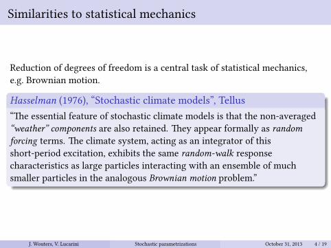
Numerical experiment (with S. Dolaptchiev & U. Achatz)

Stochastically perturbed additive triadFast Ornstein-Uhlenbeck process (y) coupled to a slow variable (x) bynonlinear coupling

dxdt = B0y1y2dy1dt = B1y2x− γ1

ϵ y1 +σ1√ϵU

dy2dt = B2xy1 − γ2

ϵ y2 +σ2√ϵV

→

dxdτ = ϵB0y1y2dy1dτ = ϵB1y2x− γ1y1 + σ1Udy2dτ = ϵB2xy1 − γ2y2 + σ2V

τ = tϵ

Homogenisation results in an Ornstein-Uhlenbeck process

J. Wouters, V. Lucarini Stochastic parametrizations October 31, 2013 14 / 19

Numerical experiment: weak coupling

e parametrization can be explicitly computed

CΨx;Ψx(s) = ⟨Ψx(y(t))Ψx(y(t+ s))⟩= (ϵB(0))2⟨y1(t)y2(t)y1(t+ s)y2(t+ s)⟩∼ e−(γ1+γ2)s

RΨx;Ψy(s) = ⟨Ψy(x(t), y(t))∇yΨx(y(t+ s))⟩= ⟨ϵB(1)y2x∂y1(ϵB(0)y1(t+ s)y2(t+ s))⟩+ (1 ↔ 2)

∼ e−(γ1+γ2)s

J. Wouters, V. Lucarini Stochastic parametrizations October 31, 2013 15 / 19

Numerical experiment: results

Autocorrelation of x for ϵ = 0.125

0 2 4 6 8 10 12 14 160

0.1

0.2

0.3

0.4

0.5

0.6

0.7

0.8

0.9

1normalized ACF, eps=0.125

full

weak

hom

t

J. Wouters, V. Lucarini Stochastic parametrizations October 31, 2013 16 / 19

Numerical experiment: results

Autocorrelation of x for ϵ = 0.25

0 1 2 3 4 5 6 7 8�0.2

0

0.2

0.4

0.6

0.8

1

1.2normalized ACF, eps=0.25

full

weak

hom

t

J. Wouters, V. Lucarini Stochastic parametrizations October 31, 2013 17 / 19

Numerical experiment: results

Autocorrelation of x for ϵ = 0.5

0 0.5 1 1.5 2 2.5 3 3.5 4�0.2

0

0.2

0.4

0.6

0.8

1

1.2normalized ACF, eps=0.5

full

weak

hom

t

J. Wouters, V. Lucarini Stochastic parametrizations October 31, 2013 18 / 19

Conclusions

In reduced models, correlated noise and memory appearCorrelation function and memory kernel can be determined in theuncoupled Y system.Preliminary numerical experiments show encouraging results.

Response: Wouters, Lucarini (2012) J. Stat. Mech.Mori-Zwanzig: Wouters, Lucarini (2013) J. Stat. Phys.

ank you!

J. Wouters, V. Lucarini Stochastic parametrizations October 31, 2013 19 / 19